Joint power spectrum and voxel intensity distribution forecast on the CO luminosity function with COMAP

Abstract

We develop a framework for joint constraints on the CO luminosity function based on power spectra (PS) and voxel intensity distributions (VID), and apply this to simulations of COMAP, a CO intensity mapping experiment. This Bayesian framework is based on a Markov chain Monte Carlo (MCMC) sampler coupled to a Gaussian likelihood with a joint PS + VID covariance matrix computed from a large number of fiducial simulations, and re-calibrated with a small number of simulations per MCMC step. The simulations are based on dark matter halos from fast peak patch simulations combined with the $L_{\text{CO}}(M_{\text{halo}})$ model of Li et al. (2016). We find that the relative power to constrain the CO luminosity function depends on the luminosity range of interest. In particular, the VID is more sensitive at large luminosities, while the PS and the VID are both competitive at small and intermediate luminosities. The joint analysis is superior to using either observable separately. When averaging over CO luminosities ranging between $L_{\text{CO}}=10^{4}-10^{7}L_{\odot}$, and over 10 cosmological realizations of COMAP Phase 2, the uncertainties (in dex) are larger by 58% and 30% for the PS and VID, respectively, when compared to the joint analysis (PS + VID). This method is generally applicable to any other random field, with a complicated likelihood, as long a fast simulation procedure is available.

1 Introduction

Intensity mapping (Madau et al. 1997; Battye et al. 2004; Peterson et al. 2006; Loeb & Wyithe 2008) appears promising for mapping large 3D volumes cheaply in a relatively short period of time, using specific bright emission lines as matter tracers. This is an interesting avenue for advancing precision cosmology, with a multitude of ongoing efforts (Kovetz et al. 2017), following on the successes of the CMB field in the last few decades. One such line intensity mapping experiment currently under construction is called the CO Mapping Array Pathfinder (COMAP; Cleary et al. 2016; Li et al. 2016), which aims to observe frequencies between 26 and 34 GHz, corresponding to redshifted CO line emission from the epoch of galaxy assembly (redshifts between $z=2.4$ and 3.4) for the CO $J$=1$\rightarrow$0 line at 115 GHz rest frequency, and CO emission from the epoch of reionization ($z=5.8$–6.7) for the CO $J$=2$\rightarrow$1 line at 230 GHz rest frequency.

One important scientific target for studying and understanding the epoch of galaxy assembly, the main goal of the first COMAP phase, is the so-called CO luminosity function, which measures the number density of CO emitters as a function of luminosity. Several methods for extracting this function from real data have already been suggested in the literature, and the most prominent of these is the power spectrum (PS) approach, for instance as implemented by Li et al. (2016). A second complementary method is the 1-point function, or voxel intensity distribution (VID), $\mathcal{P}(T)$, as suggested by Breysse et al. (2017, 2016).

In this paper, we consider the prospect of combining the VID and PS approaches when constraining the CO luminosity function, and we study this approach within the context of the COMAP experiment. To do so, we first define a joint likelihood that includes both the VID and the PS, and construct a joint covariance matrix for both observables. This covariance matrix is constructed from a large set of dark matter (DM) light-cone halo catalogs from so-called “peak patch” cosmological simulations Bond & Myers (1996); Stein et al. (2018), coupled to an empirical $L_{\mathrm{CO}}(M_{\text{halo}})$ model (Li et al. 2016) that infers CO luminosities, $L_{\mathrm{CO}}$, from DM halo masses, $M_{\text{halo}}$. We then investigate the posterior distribution of the resulting model parameters for each of the first two anticipated phases of the COMAP experiment (see Table 1). Finally, we compare the constraints on the CO luminosity function derived from joint PS and VID measurements to those obtained from the PS or VID separately.

2 Idealized simulations of the COMAP experiment

Table 1: Experiment setup for the two COMAP phases.

Parameter      COMAP1 COMAP2 System temperature, $$T_{\text{sys}} \delta\nu \mu$$ [K] .      40 40 Number of feeds .      19 95 Beam FWHM (arcmin) .      4 4 Frequency band [GHz] .      26–34 26–34 Channel width, (MHz) .      15.6 15.6 Observing time [h] .      6000 9000 Noise per voxel [K] .      11.0 8.0 Field size [deg²] .      2.25 2.25 Number of fields .      1 4

We start our discussion by reviewing some central properties of the COMAP experiment, focusing in particular on those required for generating representative yet computationally affordable simulations. For convenience, these properties are summarized in Table 1.

In Phase 1 COMAP will employ a single telescope equipped with 19 single-polarization detectors, each with 512 frequency channels with width $\delta\nu\approx$ 15.6 MHz covering frequencies between 26 GHz and 34 GHz. The system temperature is expected to be around $T_{\text{sys}}\approx 40$ K, and the angular resolution corresponding to a Gaussian beam with $4^{\prime}$ full width at half maximum (FWHM). We anticipate two years of observation time targeting a single field of 1.5 deg $\times$ 1.5 deg close to the north celestial pole, and we assume a conservative observing efficiency of 35%, for a total of 6000 hours of total integration time on the field.

In Phase 2, the experiment will be expanded to five telescopes with the same setup as in Phase 1, and observe for three additional years. In this phase, we assume that the observation time will be split between four fields of the same size as in Phase 1. The two COMAP phases will be referred to as COMAP1 and COMAP2 in the following.

2.1 Noise

The simulations used in this work consist of two components only, namely the target CO signal and random white noise with properties corresponding to the parameters described above. Explicitly, the noise per voxel, is given by

$$\sigma_{T}=\frac{T_{\text{sys}}}{\sqrt{\tau\thinspace\delta\nu}}=\frac{T_{\text{sys}}\sqrt{N_{\text{pixels}}}}{\sqrt{\tau_{\text{tot}}e_{\text{obs}}N_{\text{feeds}}\delta\nu}},$$ (1)

where $T_{\text{sys}}$ is the system temperature, $\tau$ is the observation time per pixel, $\tau_{\text{tot}}$ is the total observation time , $e_{\text{obs}}$ is the observation efficiency, $N_{\text{feeds}}$ is the number of feeds, $N_{\text{pixels}}$ is the number of pixels, and $\delta\nu$ is the frequency resolution. This gives us $\sigma_{T}\approx 11\thinspace\mu\text{K and }8\thinspace\mu\text{K}$, for the COMAP1 and COMAP2 phases respectively. For simplicity we assume that the noise is evenly distributed over all voxels.

A voxel is the 3D equivalent of a pixel. Two of the dimensions correspond to a regular pixel on the sky, while the third dimension corresponds to a small range of redshifts from where line emmision would redshift into a given frequency bin of our instrument.

Both instrumental systematics and astrophysical foreground contamination are neglected in the following. However, since our estimator is inherently simulation-based, these effects can be added at a later stage, when a sufficiently realistic instrument model is available. For discussion of foreground contamination in similar line intensity surveys see e.g. da Cunha et al. (2013); Breysse et al. (2015, 2017); Chung et al. (2017).

2.2 Dark matter simulations

The signal component is based on the peak patch DM halo approach described by Bond & Myers (1996); Stein et al. (2018), coupled to the $L_{\mathrm{CO}}(M_{\text{halo}})$ model presented by Li et al. (2016). Additionally, we adopt the same cosmological parameters as the Li et al. (2016) analysis for the dark matter simulations: $\Omega_{m}=0.286$, $\Omega_{\Lambda}=0.714$, $\Omega_{b}=0.047$, $h=0.7$, $\sigma_{8}=0.82$, and $n_{s}$ = 0.96.

The DM simulations in this paper were created using the peak patch method of Bond & Myers (1996); Stein et al. (2018). To cover the full redshift range of the COMAP experiment we simulated a volume of (1140 Mpc)³ using a particle-mesh resolution of $N_{\textrm{cells}}=4096^{3}$. Projecting this onto the sky results in a $9.6^{\circ}\times 9.6^{\circ}$ field of view covering the redshift range $2.4<z<3.4$, with a minimum dark matter halo mass of 2.5$\times$10${}^{10}M_{\odot}$.

The resulting halo catalog contains roughly 54 million halos, each with a position, a velocity, and a mass. The peak patch method can simulate continuous light-cones on-the-fly, so stitching snapshots together was not required to create the light-cone. Although peak patch simulations result in quite accurate halo masses, the dark matter halo catalogs were additionally mass corrected by abundance matching along the lightcone to Tinker et al. (2008) to ensure statistically the same mass function as the simulations used in the Li et al. (2016) analysis. For a detailed study of the clustering properties of peak patch simulations and other approximate methods see Lippich et al. (2018); Blot et al. (2018); Colavincenzo et al. (2018).

A single run required 900 seconds of compute time on 2048 Intel Xeon EE540 2.53 GHz CPU cores of the Scinet-GPC cluster, with a memory footprint of $\simeq$ 2.4 TB. This efficiency of the peak patch method allowed for 161 independent realizations of the full 1140Mpc, $N_{\textrm{cells}}=4096^{3}$ volume, taking a total compute time of only $\sim$ 82,000 CPU hours, over 3 orders of magnitude faster when compared to an N-body method of equivalent size.

2.3 Converting to CO brightness temperature

There are many approaches in the literature for estimating the expected CO signal based on DM halos (e.g. Righi et al. 2008; Obreschkow et al. 2009; Visbal & Loeb 2010; Lidz et al. 2011; Carilli 2011; Gong et al. 2011; Fu et al. 2012; Pullen et al. 2013; Carilli & Walter 2013; Breysse et al. 2014; Greve et al. 2014; Mashian et al. 2015; Li et al. 2016; Padmanabhan 2018), with resulting estimates of the CO-luminosities spanning roughly an order of magnitude.

Here we adopt the model described by Li et al. (2016), to convert from simulated light-cones populated with DM halos to observed CO brightness temperature. This model is defined by a set of parametric relations between DM halo masses, star formation rates (SFR), infrared (IR) luminosities, $L_{\text{IR}}$, and CO-luminosities, $L_{\text{CO}}$.

The model uses the results from Behroozi et al. (2013a, b) to obtain average SFR from DM halo masses, and adds an additional log-normal scatter on top of the average, determined by $\sigma_{\mathrm{SFR}}$. IR luminosities are then obtained through the relation

$$\mathrm{SFR}=\delta_{\mathrm{MF}}\times 10^{-10}L_{\mathrm{IR}}.$$ (2)

Further, to obtain CO luminosities, the relation

$$\log L_{\mathrm{IR}}=\alpha\log L^{\prime}_{\mathrm{CO}}+\beta,$$ (3)

is used before a second round of log-normal scatter is added, determined by the parameter $\sigma_{L_{\mathrm{CO}}}$.

This gives us a $L_{\mathrm{CO}}(M_{\mathrm{halo}})$ model with five free parameters, $\theta=\{\sigma_{\mathrm{SFR}},\log\delta_{\text{MF}},\alpha,\beta,\sigma_{L_{\mathrm{CO}}}\}$. The relation between $L_{\mathrm{CO}}$ and $M_{\text{halo}}$, for our fiducial model parameters, is shown in Figure 1. For more discussion of the physical and observational motivation for this model, see the original paper Li et al. (2016).

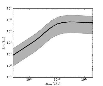
Figure 1: Plot of CO luminosity, $L_{\mathrm{CO}}$, as a function of dark matter halo mass, $M_{\text{halo}}$, in the Li et al. (2016) model. Here $(\sigma_{\mathrm{SFR}},\log\delta_{\text{MF}},\alpha,\beta,\sigma_{L_{\mathrm{CO}}})=(0.3,0.0,1.17,0.21,0.3)$ (our fiducial model), and we have evaluated the function at redshift $2.9$. The solid line corresponds to the mean relation with no scatter added, while the shaded region corresponds to the $95\%$ confidence intervals after adding log-normal scatter at the two appropriate steps.

This model is applied to each DM halo separately, and from the resulting CO luminosities we create high-resolution maps by converting the total luminosity in a given voxel into brightness temperature. These maps were created using the publicly available limlam_mocker code. Next, we convolve these maps with the (Gaussian) instrumental beam profile, degrade to the low-resolution voxel size used in the analysis, and, finally, we add Gaussian uncorrelated noise with standard deviation $\sigma_{T}$ as specified above.

3 Algorithms

The ultimate goal of this work is to constrain cosmological and astrophysical parameters from CO line intensity observations. The computational engine for this work is a standard Metropolis Markov chain Monte Carlo (MCMC) sampler (see e.g., Gilks et al. 1995), coupled to a posterior distribution with a corresponding likelihood and prior. For this task to be computationally tractable, though, the full CO line intensity data set must first be compressed to a smaller set of observables that may be modeled in terms of the desired astrophysical parameters, fully analogous to how CMB sky maps are compressed to a CMB power spectrum from which cosmological parameters are derived (e.g., Bond et al. 2000). As described above, we adopt the power spectrum and the voxel intensity distribution as representative observables, each of which may be approximated in terms of multivariate Gaussian random variables. However, in order to perform a joint analysis of these two observables, we need to construct their joint covariance matrix, and that is the primary goal of this section. Before doing that, however, we review for completeness each observable individually, and our posterior sampler of choice, referring to relevant literature for full details.

3.1 The power spectrum

The estimated power spectrum, $P(k_{i})$, is calculated simply by taking the 3D Fourier transform of the temperature cube, binning the absolute squared values of the Fourier coefficients according to the magnitude of corresponding wave number $k$, and averaging over all the contributions within each bin. For a Gaussian map, the Fourier components within each bin follow a perfect normal distribution with mean zero and variance given by the value of the power spectrum. For a non-Gaussian field the distribution of the Fourier components is more complicated, and thus the power spectrum does not contain all the statistical information in the map. We expect the CO signal to form a highly non-Gaussian map, therefore, in this paper, we simply consider the power spectrum as a useful observable that carries some, but far from all, of the statistical information in the map.

As an observable, the power spectrum needs to be accompanied by a covariance matrix $\xi^{P}_{ij}\equiv\text{Cov}(P(k_{i}),P(k_{j}))$ in the analysis, since there are correlations between the power spectrum at different $k$-values.

3.2 The voxel intensity distribution

We consider the VID as another observable, complementary to the PS, and more closely related to the luminosity function.

We do not, unlike in many other works on $\mathcal{P}(D)$ analysis (e.g. Lee et al. (2009); Glenn et al. (2010); Vernstrom et al. (2014); Breysse et al. (2017); Leicht et al. (2018)), try to estimate the VID analytically, rather we estimate it based on simulations. This allows us to fully take into account the effects of the beam, clustering and covariance between temperature bins in a very straightforward manner.

We consider two contributions to the VID, namely the CO signal itself and the instrumental noise. Together they result in the the full probability distribution of voxel temperatures, $\mathcal{P}(T)$, where $T$ is the observed brightness temperature from a voxel. Since we, in this paper, assume the noise to be uniformly distributed over all voxels in the observed field, and the CO signal itself is statistically homogeneous and isotropic, the total probability distribution, $\mathcal{P}(T)$, is the same across all voxels.

The basic observable related to the VID are the temperature bin counts (i.e. the histogram of voxel temperatures), $B_{i}$. The expectation value of these are given by the VID itself,

$$\langle B_{i}\rangle=N_{\text{vox}}\int_{T_{i}}^{T_{i+1}}\mathcal{P}(T)dT,$$ (4)

where $N_{\text{vox}}$ is the number of voxels observed and $B_{i}$ is the number of voxels with a temperature between $T_{i}$ and $T_{i+1}$.

If the temperatures of all the voxels that we sample were completely independent, then each of the voxel bins would be approximately independent, and follow a binomial distribution with variance $\text{Var}_{\text{ind}}(B_{i})=\langle B_{i}\rangle(1-\langle B_{i}\rangle/N_{\text{vox}})$. However, even in this ideal case they would not be perfectly independent. We only have a finite number of voxels, and, therefore, if one bin contains a number of voxels above average, then the other bins must have a number of bins lower than the average.

In general, the samples will not be independent for many reasons, including correlated sky or noise structures and processing effects, and we therefore need the full covariance matrix between bins, $\xi^{B}_{ij}\equiv\text{Cov}(B_{i},B_{j})$. This covariance matrix will depend on the DM density field, the CO bias, and the luminosity function, and we will estimate it using simulations.

3.3 The joint PS+VID covariance matrix

The main missing component in the above method is definition of a joint power spectrum and voxel intensity distribution covariance matrix. By having access to the computationally cheap yet realistic Monte Carlo simulations described above, we can approximate this matrix by simulations. In addition to giving us covariance matrices to do our analysis, this also allows us to check under what conditions the full covariance matrix is necessary, and when we can get away with assuming that individual samples are independent.

In this paper, we start out with 161 independent simulated light-cone cubes of dark matter halos, each covering about $9.6^{\circ}\times 9.6^{\circ}$ on the sky, and a frequency range between 26 and 34 GHz, corresponding to redshifts between 2.4 and 3.4. The frequency dimension is divided equally into 512 frequency bins, each spanning $\delta\nu\approx 15.6~{}\mathrm{MHz}$, corresponding to a redshift resolution of $\delta z\approx 0.002$. Since the COMAP field only spans $1.5^{\circ}\times 1.5^{\circ}$ on the sky, we sub-divide each of the $9.6^{\circ}\times 9.6^{\circ}$ light-cone cubes, after beam convolution, into 36 square fields each covering $1.5^{\circ}\times 1.5^{\circ}$ , resulting in a total of 5796 semi-independent sky realizations. The final pixelisation of these maps is a $22\times 22$ grid of square pixels, resulting in a pixel size of $\delta\theta\approx 4.1^{\prime}$. To these maps, we add uniformly distributed white noise at the appropriate levels for the COMAP1 and COMAP2 experiment setups described above.

When choosing the pixel size to use for the analysis, we follow Vernstrom et al. (2014). They show that, for $\mathcal{P}(D)$ analysis, choosing a pixel size to be equal to the FWHM of the beam is a good trade-off between picking a small pixel size to include the maximal information, and choosing a larger pixel size to reduce the pixel to pixel correlations induced by the beam.

We combine our two observables into a joint one-dimensional vector of the form

$$d_{i}=(P_{k_{i}},B_{i}),$$ (5)

where $P_{k_{i}}$ is the binned power spectrum, and $B_{i}$ are the temperature bin counts. Let us first consider the ideal case in which all elements in this vector are independent, and the Fourier components are approximately Gaussian. In that case we can compute the expected variance, which we will simply call the independent variance, analytically,

$$\text{Var}_{\text{ind}}(P_{k_{i}}) =\langle P_{k_{i}}\rangle^{2}/N_{\text{modes}}(k_{i}),$$ (6)

$$\text{Var}_{\text{ind}}(B_{i}) =\langle B_{i}\rangle(1-\langle B_{i}\rangle/N_{\text{vox}})\approx\langle B_{i}\rangle,$$ (7)

where $N_{\text{modes}}(k_{i})$ is the number of modes in the $i^{\text{th}}$ $k-$bin and where we have introduced the notation $\text{Var}_{\text{ind}}(d_{i})$ for this conditionally independent variance.

With this notation in hand, we define a “pseudo-correlation matrix” as

$$c_{ij}\equiv\frac{\xi_{ij}}{\sqrt{\text{Var}_{\text{ind}}(d_{i})\text{Var}_{\text{ind}}(d_{j})}},$$ (8)

where, as in Sect. 3.4, $\xi_{ij}$ is the full covariance matrix. Note that $c_{ij}$ is the exact correlation matrix in the limit that $\text{Var}_{\text{ind}}(d_{i})$ is the true full variance. An important advantage of the pseudo-correlation matrix, however, is the fact that $\text{Var}_{\text{ind}}(d_{i})$ may be estimated directly from the average data itself, and this is required for our MCMC procedure to be sufficiently fast.

The full covariance matrix $\xi$ is estimated for the model described by Li et al. (2016), adopting the fiducial parameters $\theta_{0}$, using the set of 5796 simulations described above. However, for the MCMC sampler described in Sect. 3.4, we actually need the full covariance matrix, corresponding to different model parameters $\theta$, at each step in the Markov chain. Generating the full covariance matrix with the above procedure at each MC step is clearly not computationally feasible, and we therefore need to approximate this somehow.

With regard to this last point, we introduce the following proposal: we assume that the full covariance matrix scales, under a change of model parameters from $\theta_{0}$ to $\theta$, the same way as the independent variance, $\text{Var}_{\text{ind}}(d_{i})$, does

$$\hat{\xi}_{ij}(\theta)\approx\xi_{ij}(\theta_{0})\frac{\sqrt{\text{Var}_{\text{ind}}^{\theta}(d_{i})\text{Var}_{\text{ind}}^{\theta}(d_{j})}}{\sqrt{\text{Var}_{\text{ind}}^{\theta_{0}}(d_{i})\text{Var}_{\text{ind}}^{\theta_{0}}(d_{j})}},$$ (9)

where $\text{Var}_{\text{ind}}^{\theta_{0}}(d_{i})$ is the independent variance for the fiducial model, and $\text{Var}_{\text{ind}}^{\theta}(d_{i})$ is the independent variance for arbitrary parameters $\theta$. Since this latter function only depends on the average quantities $\langle d_{i}\rangle$, it is computationally straightforward to compute $\hat{\xi}_{ij}(\theta)$ at any position in a MCMC sampler. Note also that $\hat{\xi}_{ij}(\theta)$ is, by construction, positive definite, as required for a proper covariance matrix.

For a noise dominated experiment, where all samples are approximately independent, the independent variance, $\text{Var}_{\text{ind}}(d_{i})$, is the correct variance, and Eq. 9 is the correct scaling of the covariance matrix. However, we use this scaling as a first approximation even in cases where there is some covariance in the data.

Intuitively, Eq. 9 is equivalent to postulating that the pseudo-correlation matrix, $c_{ij}$, is approximately constant (i.e. independent of the specific parameters in question). For real-world applications, we recommend testing this assumption explicitly by computing the covariance matrix by brute force simulation for a few extreme parameter combinations drawn from the Markov chains produced during the analysis.

The above prescription applies straightforwardly to single-field observations as, for instance, planned for COMAP1. In contrast, COMAP2 will, under our assumptions, span $N=4$ independent but statistically identical fields. Since the mean vector of observables evaluated across those four fields equals the average of the four corresponding independent observable vectors, the full covariance matrix is simply given by the single field covariance matrix divided by the number of fields:

$$\xi_{ij}^{N\thinspace\mathrm{field}}=\frac{\xi_{ij}^{\text{1 field}}}{N}.$$ (10)

Note that $c_{ij}$ then, assuming the fields are of the same size, only depends on the noise level per field, so for a given noise level per field, $c_{ij}$ is independent of the number of fields.

Finally, we note that the total number of degrees of freedom in our joint PS+VID statistic is in this paper equal to 45, corresponding to 20 power spectrum bins and 25 VID bins. For this number of degrees of freedom, a set of 5796 (semi-independent) simulations provides a very good estimate of all numerically dominant components of the covariance matrix, including both the diagonal and the leading off-diagonal modes, and $\xi_{ij}$ is well conditioned.

3.4 Posterior mapping by MCMC

As previously mentioned, we use a MCMC algorithm to sample from the posterior distribution of the $L_{\mathrm{CO}}(M_{\text{halo}})$ model parameters, $\theta=\{\sigma_{\mathrm{SFR}},\log\delta_{\text{MF}},\alpha,\beta,\sigma_{L_{\mathrm{CO}}}\}$. This posterior distribution is, as usual, given by Bayes’ theorem,

$$P(\theta|d)\propto P(d_{i}|\theta)P(\theta),$$ (11)

where $d$ represents our compressed data set, $P(d|\theta)$ is the likelihood defined below, and $P(\theta)$ is some set of priors. We use the emcee package (Foreman-Mackey et al. 2013) and its implementation of an affine-invariant ensemble MCMC algorithm, with 142 walkers.

We use a burn-in period of 1000 steps, and use the next 1000 steps for the posterior estimation.

We assume a Gaussian likelihood for our observables $d_{i}$ of the form (up to an additive constant)

$$-2\ln P(d|\theta)=\sum_{ij}[d_{i}-\langle d_{i}\rangle](\xi^{-1})_{ij}[d_{j}-\langle d_{j}\rangle]+\ln|\xi|,$$ (12)

where the means $\langle d_{i}\rangle$ depend on the model parameters $\theta$, and the covariance matrix $\xi_{ij}$ is approximated by the expression given in Eq. 9. (Note that we do not need to assume that the low-level data are Gaussian, but only that the compressed observables may be well approximated by a multi-variate Gaussian distribution. Due to the central limit theorem, this is in practice very often an excellent approximation.)

For both the power spectrum and the low and intermediate temperature VID bins, for which there is a large number of voxel counts per bin, this Gaussian approximation holds to a high degree. However, for the highest VID temperature bins, where there are only a few voxel counts per bin, the discrete nature of the bin count may become relevant, and the full binomial distribution should in principle be taken into account. This effect can however also be remedied easily by increasing the bin width, albeit at the cost of slight loss of information, as is suggested in Vernstrom et al. (2014), and we therefore neglect it in the following, as our primary focus is the dominant Gaussian component of the likelihood. A more thorough analysis may take this issue into account either analytically or by simulations.

An advantage of using a Gaussian likelihood for the VID, is that it gives us a straightforward way to take into account the correlations between temperature bins apparent in the covariance matrix, $\xi_{ij}$ (e.g. in Figure 2). For another approach to building up a $\mathcal{P}(D)$ likelihood, see Glenn et al. (2010).

To estimate $\langle d_{i}\rangle$, we compute 10 maps of the survey volume at each step in the MCMC chain, using the current model parameters $\theta$ with different dark matter halo realizations (randomly drawn from 252 independent catalogs corresponding to the survey volume). The specific number of realizations, 10 in our case, represents a compromise between minimizing the sample variance in the estimate of $\langle d_{i}\rangle$ and maintaining a reasonable computational cost per MC step. Finally, we bin all the halos in the 10 realizations according to their luminosity, and use this histogram to estimate the luminosity function at the current values of $\theta$. This way the MCMC precedure gives us the luminosity function at different points in parameter space, sampled according to the posterior of the model parameters, which we can use to derive constraints on the luminosity function itself.

We adopt the same physically motivated priors as discussed by Li et al. (2016). Specifically, these read

$$P(\sigma_{\mathrm{SFR}}) =\mathcal{N}(0.3,0.1)$$ (13)

$$P(\log\delta_{\text{MF}}) =\mathcal{N}(0.0,0.3)$$ (14)

$$P(\alpha) =\mathcal{N}(1.17,0.37)$$ (15)

$$P(\beta) =\mathcal{N}(0.21,3.74)$$ (16)

$$P(\sigma_{L_{\mathrm{CO}}}) =\mathcal{N}(0.3,0.1),$$ (17)

where $\mathcal{N}(\mu,\sigma)$ corresponds to a Gaussian distribution with mean $\mu$ and standard deviation $\sigma$. Additionally, we require the two logarithmic scatter parameters, $\sigma_{\mathrm{SFR}}$ and $\sigma_{L_{\mathrm{CO}}}$, to be positive. We choose the mean of all these distributions as the fiducial model, $\theta_{0}$.

To quantify the importance of joint PS+VID analysis, we perform the above analysis both with each observable separately, and with the joint analysis. The main result in this paper may then be formulated in terms of the relative improvement on the CO luminosity function uncertainty derived from the joint analysis to those found in the independent analyses.

When calculating our observables (PS and VID), we assume that our survey volume can be treated as a rectangular grid of voxels with constant co-moving volume. We also neglect the evolution of our observables over redshifts between $z=2.4$ and $3.4$. That is, we assume that samples from different redshifts are drawn from the same distribution, whether they are power spectrum modes or voxel temperatures. We also assume that the instrument beam is achromatic, and equal to the value at the central frequency. This is of course just an approximation that we make in order for the analysis to be simple. If we were doing experiments with higher signal to noise, we might divide our data into two different redshift regions and do an independent analysis of each region. This could allow us to study the redshift evolution of the observables. For COMAP (1 and 2), however, we are probably best off combining all the data, like we do here, in order to increase the overall signal to noise.

Finally, since COMAP will not measure absolute zero-levels, we subtract the mean from all maps. For the power spectrum, this has a negligible impact, as it simply removes one out of $N_{\mathrm{vox}}$ modes. However, for the VID it has a significantly higher impact. Specifically, it makes it much harder to distinguish a potential background of weak sources from noise. Indeed, as shown by Breysse et al. (2017), removing the monopole makes it much harder to detect a possible low luminosity cutoff in the CO luminosity function using the VID.

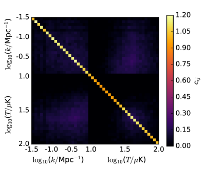
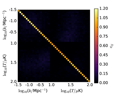
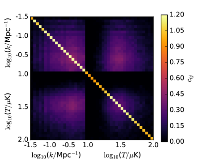
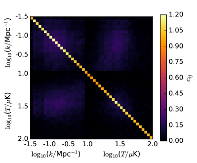
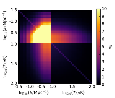
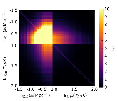
Figure 2: Estimated pseudo-correlation matrix of observables $d_{i}$, $c_{ij}=\text{Cov}(d_{i},d_{j})/(\sqrt{\text{Var}_{\text{ind}}(d_{i})\text{Var}_{\text{ind}}(d_{j})})$, based on simulated maps with and without noise. The first block in each matrix corresponds to the power spectrum, and the second block to the VID. Top: Signal plus white noise corresponding to the COMAP1 experiment ($\sigma_{\text{voxel}}\approx 11\thinspace\mu$K). Middle: Signal plus white noise corresponding to the COMAP2 experiment ($\sigma_{\text{voxel}}\approx 8\thinspace\mu$K). Bottom: Signal alone. Note that here we have changed the color scale. Left: Covariance matrices without beam smoothing. Right: Covariance matrices with $\theta_{\text{FWHM}}=4^{\prime}$ beam smoothing.

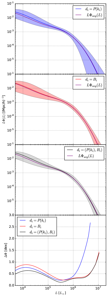
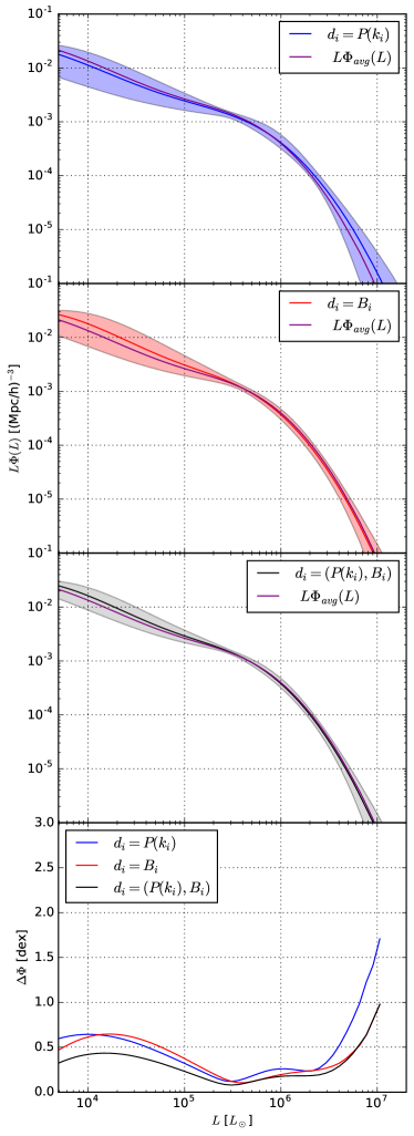
Figure 3: Constraints on the luminosity function from simulated experiments COMAP1 (left) and COMAP2 (right). The shaded area corresponds to 95% credibility intervals, solid lines correspond to the median, while the purple curve corresponds to the average luminosity function derived from all the available halo catalogs (i.e. the ensemble mean). Top: Constraints derived using only the power spectrum $P(k_{i})$ as the observable. 2. row: Constraints derived using only the temperature bin counts $B_{i}$ as the observable. 3. row: Constraints derived by a joint analysis using both the power spectrum $P(k_{i})$ and the temperature bin counts $B_{i}$ as observables. Bottom: Comparison of the uncertainty of the luminosity function constraints in dex, i.e. $\Delta\Phi\equiv\log_{10}\Phi_{\mathrm{97.5\%}}-\log_{10}\Phi_{\mathrm{2.5\%}}$.

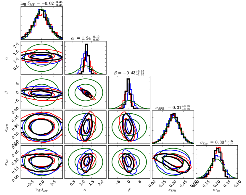
Figure 4: Posterior distributions for the Li et al. (2016) model parameters for a single realization of the COMAP2 experiment (the same realization as the COMAP2 results in Figure 3). Results for PS, VID and joint PS+VID analysis are shown in blue, red and (slightly bolder) black respectively. Prior distributions are shown in green. The two curves of each color correspond 68% and 95% credibility regions. The numbers on top of each colum correspond to the 68% credibility interval for each parameter from the PS+VID analysis. We see that while the posterior of the two scatter parameters, $\sigma_{\mathrm{SFR}}$ and $\sigma_{L_{\mathrm{CO}}}$ is mostly set by the prior, the posterior on $\log\delta_{\text{MF}}$, from the SFR-$L_{\mathrm{IR}}$ relation, is actually slightly wider than the prior, suggesting a significant intrinsic scatter in estimates of this parameter. These results are consistent with the corresponding results in Figure 7 in Li et al. (2016). The two parameters that are actually strongly constrained by the simulated experiment are $\alpha$ and $\beta$, the two parameters from the $L_{\mathrm{CO}}$-$L_{\mathrm{IR}}$ relation, and this figure shows that, at least for this realization, the constraints on these two get significantly improved in the combined analysis (PS+VID) as compared to analysis using the individual observables. This figure was created using the publicly available code^a corner (Foreman-Mackey 2016).

^a https://github.com/dfm/corner.py

4 Results

We are now ready to present the main numerical results from our analysis, and we start with an inspection of the joint PS+VID covariance matrix itself.

4.1 Visual inspection of the PS+VID covariance matrix

Figure 2 shows the pseudo-correlation matrices, $c_{ij}$, for our two experimental setups, as well as for pure signal alone, for reference. In order to illustrate the effect of the beam, we show covariance matrices from maps both without and with beam smoothing in the left and right columns, respectively.

The first thing to notice is that instrumental noise significantly reduces the numerical values of the normalized covariance matrices, bringing it closer to the independent white noise case for which $c_{ij}=\delta_{ij}$. This agrees with intuition, since the noise itself is white and uncorrelated.

Beam smoothing also leads to weaker correlations. This is mainly due to the beam diluting the signal at small scales, where the correlation is otherwise strongest.

Next, we notice that the cross-correlations between the power spectrum and VID are of the same order of magnitude as the correlations internal to each observable itself. Thus, it is essential to account for all these correlations in any joint PS and VID analysis, as done in the present paper.

Finally, we note that when designing an experiment like COMAP, one of the important trade-offs involves observation time per field. To obtain a fast signal detection it is in general advantageous to observe deep on the smallest possible field. However, this only holds true while the signal-to-noise per voxel is significantly less than unity. When the noise starts to become comparable to the signal, the signal-induced voxel-voxel correlations starts to become important, and the effective uncertainties no longer scale as $\mathcal{O}(1/\sqrt{\tau})$, where $\tau$ is the observation time per pixel. Generally, in such a tradeoff, any significant correlations between different power spectrum modes or voxel temperatures will tend to favor larger survey area or multiple fields, both effectively leading to more independent samples, and thereby higher overall integration efficiency.

4.2 Luminosity function constraints

We are now ready to present both individual and joint PS+VID constraints on the CO luminosity function, and these are summarized in Figure 3 for COMAP1 (left column) and COMAP2 (right column). The top row shows the constraints obtained from the power spectrum alone; the middle row shows the constrains obtained from the VID alone; and the third row shows the constraints from the joint analysis. In each panel, the shaded colored region shows the 95% credibility region from the MCMC samples, and the solid line with the same color shows the posterior median. The purple solid line shows the average luminosity function obtained from the mean of all available halo catalogs, and thus represents the ensemble average of our input model. Note that the colored regions correspond to one single realization, and the uncertainties therefore contain contributions from instrumental noise, cosmic variance and sample variance. The agreement between the estimated confidence regions and the ensemble mean is quite satisfactory in all cases, with uncertainties that appear neither too large nor too small.

Considering first the individual PS and VID estimates, shown in the top two rows, we see that the two observables are indeed complementary. In particular, the VID primarily constrains the high luminosity end of the luminosity function, while the power spectrum imposes relatively stronger constraints on the low luminosity end. This makes sense intuitively, since the VID is essentially optimized to look for strong outliers above the noise, whereas the power spectrum represents a weighted mean across the full field for each physical scale. It is interesting to note, however, that the VID provides, on average, stronger constraints on the luminosity function than the power spectrum does.

Due to this complementarity, the joint estimator provides the strongest constraints of all. To make this point more explicit, the fourth row compares the uncertainties of the independent power spectrum and VID analyses to the joint constraints. Of course, there is a significant amount of cosmic variance in each of these functions, and the precise numerical value of the uncertainty ratio therefore varies significantly with luminosity; but the mean trend is clear: The individual analyses typically result in 20–70% larger uncertainties than the joint analysis when averaged over luminosities between $L_{\text{CO}}=10^{4}-10^{7}L_{\odot}$. Over 10 cosmological realizations the PS and VID resulted in, on average, 58% and 30% larger uncertainties (in dex) individually, than the joint analysis. This is the main novel result presented in this paper.

4.3 Posterior distribution of model parameters

Lastly we present the constraints of the model parameters themselves. When doing the MCMC posterior mapping we explore the parameter space of the Li et al. (2016) $L_{\textrm{CO}}(M_{\textrm{Halo}})$ model. Figure 4 shows the posterior distribution for these parameters derived from one realization of the COMAP2 experiment (the same realization as the COMAP2 results in Figure 3).

Results for PS, VID and joint PS+VID analysis are shown in blue, red and black respectively. Prior distributions are shown in green. The two curves of each color correspond 68% and 95% credibility regions.

We see that the two parameters that are mainly constrained are $\alpha$ and $\beta$, the two parameters from the average $L_{\mathrm{CO}}$- $L_{\mathrm{IR}}$ relation. These two parameters are fairly degenerate, and the direction in which they are degenerate is given roughly by the line $\alpha=-0.1\beta+1.19$ (Li et al. 2016). In Figure 5 we show the luminosity function for different points on this line. For the figure, the values of $\sigma_{\mathrm{SFR}},$ $\sigma_{\mathrm{L_{\mathrm{CO}}}}$ and $\log\delta_{\text{MF}}$ are fixed at $0.3,0.3$, and $0.0$ respectively. Although the overall signal strength, at least in terms of detectability, is fairly constant along this line, the shape of the luminosity function changes significantly. Lower values of alpha imply a more steep power law relation between $L_{\mathrm{CO}}$ and $L_{\mathrm{IR}}$ leading to more sources with very high or very low luminosity. We see this as a flattening of the luminosity function. In such a case a larger fraction of the overall signal will be given by high luminosity sources.

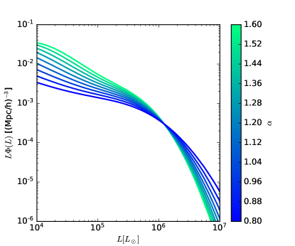
Figure 5: Plot of the CO luminosity function in the Li et al. (2016) model, for different values of $\alpha$ and $\beta$. The colors of the lines indicate the values of $\alpha$, the values of $\sigma_{\mathrm{SFR}},$ $\sigma_{\mathrm{L_{\mathrm{CO}}}}$ and $\log\delta_{\text{MF}}$ are fixed at $0.3,0.3$, and $0.0$ respectively, while the value of $\beta$ is determined from the relation $\alpha=-0.1\beta+1.19$. This line corresponds roughly to the direction along which $\alpha$ and $\beta$ are degenerate. Although the overall detectability of the signal remains roughly constant along this line, we see that the shape of the luminosity function changes significantly. We see that lower values of $\alpha$ correspond to less steep high luminosity tails in the luminosity function, meaning that a larger proportion of the overall signal comes from high luminosity sources.

The other parameter that is also slightly constrained is the log-normal scatter parameter from the $L_{\mathrm{CO}}$-$L_{\mathrm{IR}}$ relation, $\sigma_{\mathrm{L_{\mathrm{CO}}}}$. This parameter is only slightly more constrained compared to the prior, with the highest values of $\sigma_{\mathrm{L_{\mathrm{CO}}}}$ being disfavoured. The posterior of the other scatter parameter, $\sigma_{\mathrm{SFR}}$, is basically given by the corresponding prior (i.e. this parameter is not very well constrained by the experiment), although, as expected from the fact that the scatter parameters have basically the same effect, we see signs of the degeneracy between them in the posterior.

Interestingly, the normalization parameter in the SFR-$L_{\mathrm{IR}}$ relation, $\log\delta_{\text{MF}}$, actually has a posterior that is wider than the prior. This may be because the best fit of this parameter from each of the different patches have an intrinsic scatter larger than the scatter in the prior. We note that we see the same effect in Li et al. (2016) (their Figure 7).

From the mean relations in the Li et al. (2016) model we have $\log L_{\mathrm{CO}}\sim-\beta-\log\delta_{\text{MF}}$. Intuitively, we would then expect $\log\delta_{\text{MF}}$ to be completely degenerate with $\beta$. However, since the SFR-$L_{\mathrm{IR}}$ is much better constrained by observations than the $L_{\mathrm{CO}}$-$L_{\mathrm{IR}}$ relation is, the prior on $\log\delta_{\text{MF}}$ is much tighter than the one on $\beta$. The degeneracy thus prevents us from constraining $\log\delta_{\text{MF}}$ until $\beta$ is constrained to a comparable level.

5 Discussion

We have developed a joint power spectrum and voxel intensity distribution analysis for the CO luminosity function in the context of the COMAP CO intensity mapping experiment. We have implemented an efficient approach to estimating the joint covariance matrix for these two observables, and shown that accounting for both one- and two-point correlations leads to 20–70% smaller uncertainties on the CO luminosity function for both COMAP1 and COMAP2.

The critical computational engine in our approach is the construction of fast yet semi-realistic simulations of the signal in question. These simulations are based on the computationally cheap peak patch dark matter halo simulations produced by Bond & Myers (1996); Stein et al. (2018), coupled to the semi-analytic CO luminosity model of Li et al. (2016). Of course, the results we derive are correspondingly limited by how well the model reproduces the true cosmological signal. If the true signal is significantly more complex than the model predicts, the constraints in Figure 3 will not be reliable.

The strength of the constraints on the CO luminosity function will depend on the overall level of the CO signal, which is highly uncertain. However, given the same rough level of signal, we expect the constraints on the luminosity function at the high luminosities to be less model dependent than the constraints on the $L_{\mathrm{CO}}-M_{\text{halo}}$ relation or the luminosity function at lower luminosities. This is because the high luminosity sources leave a fairly unique imprint on the maps that does not depend on the specific model used.

Additionally, we expect that the relative merits of using the PS or the VID as observables will change depending on the properties of the signal. In particular, anything that increases the shot noise of the signal, like a a strong galactic duty cycle, a large intrinsic scatter in luminosities or just a more top-heavy luminosity function, will make the resulting map more non-Gaussian, tending to favor observables like the VID more as compared to the PS. We can see this effect directly in Figure 4. The VID is better, compared to the PS, at ruling out low values of $\alpha$ and high values of $\sigma_{L_{\mathrm{CO}}}$, both of which corresponds to cases where we would have a more top-heavy luminosity function and thus more shot noise.

We also expect the map to be more non-Gaussian on small scales than on large, so a wide survey with low resolution will tend to favor the PS, relative to the VID, more than a narrower high resolution survey.

While the issues of model dependence are less relevant for low signal-to-noise measurements, where we are just trying to establish the rough level of the signal, they will become more important as the measurements improve.

Another potential issue with the simulations used in this paper is the minimum dark matter halo mass of 2.5$\times$10${}^{10}M_{\odot}$. While the model used here predicts that only a small fraction of the CO signal would come from halos lighter than this (see Li et al. (2016) and Chung et al. (2017)), other models could disagree. If fact, searching for a low luminosity cutoff in the CO luminosity function is an interesting target for CO intensity mapping, and simulated halo catalogs with a smaller minimum dark matter halo mass would be useful both for forcasts and inference in such a scenario.

In general, it will be important to continuously improve the simulation pipeline as the experiment proceeds, in order to account for more and more cosmological, astrophysical and instrumental effects. However, the most important point in our approach is the fact that all such effects may be seamlessly accounted for, as long as the simulation procedure is sufficiently fast in order to be integrated into the MCMC procedure.

It should also be noted that our approach may be generalized in many different directions. For instance, the CO luminosity function does not play any unique role in our analysis, but is rather simply one specific worked example of a particularly interesting astrophysical function to be constrained. Many other functions may be constrained in a fully analogous manner, including for instance non-parametric $L_{\mathrm{CO}}(M_{\text{halo}})$ models, or any of the parameters that are involved in converting the dark matter halo distributions to CO luminosities. The method is also not specific to CO intensity mapping, but should be equally well suited for other lines, or a combination of lines (Chung et al. 2018). Indeed, it should work for any type of random fields for which the covariance matrix must be estimated by simulations. Finally, we also note that there is nothing special about the power spectrum or VID as observables, but any other efficient data compression can be equally well included in the analysis, as long as the required compression step is sufficiently computationally efficient.

References

- Battye et al. (2004) Battye, R. A., Davies, R. D., & Weller, J. 2004, MNRAS, 355, 1339
- Behroozi et al. (2013a) Behroozi, P. S., Wechsler, R. H., & Conroy, C. 2013a, ApJ, 762, L31
- Behroozi et al. (2013b) Behroozi, P. S., Wechsler, R. H., & Conroy, C. 2013b, ApJ, 770, 57
- Blot et al. (2018) Blot, L., Crocce, M., Sefusatti, E., et al. 2018, ArXiv e-prints [\eprint[arXiv]1806.09497]
- Bond et al. (2000) Bond, J. R., Jaffe, A. H., & Knox, L. 2000, ApJ, 533, 19
- Bond & Myers (1996) Bond, J. R. & Myers, S. T. 1996, ApJS, 103, 1
- Breysse et al. (2017) Breysse, P. C., Kovetz, E. D., Behroozi, P. S., Dai, L., & Kamionkowski, M. 2017, MNRAS, 467, 2996
- Breysse et al. (2014) Breysse, P. C., Kovetz, E. D., & Kamionkowski, M. 2014, MNRAS, 443, 3506
- Breysse et al. (2015) Breysse, P. C., Kovetz, E. D., & Kamionkowski, M. 2015, MNRAS, 452, 3408
- Breysse et al. (2016) Breysse, P. C., Kovetz, E. D., & Kamionkowski, M. 2016, MNRAS, 457, L127
- Carilli (2011) Carilli, C. L. 2011, ApJ, 730, L30
- Carilli & Walter (2013) Carilli, C. L. & Walter, F. 2013, ARA&A, 51, 105
- Chung et al. (2017) Chung, D. T., Li, T. Y., Viero, M. P., Church, S. E., & Wechsler, R. H. 2017, ApJ, 846, 60
- Chung et al. (2018) Chung, D. T., Viero, M. P., Church, S. E., et al. 2018, ArXiv e-prints [\eprint[arXiv]1809.04550]
- Cleary et al. (2016) Cleary, K., Bigot-Sazy, M.-A., Chung, D., et al. 2016, in American Astronomical Society Meeting Abstracts, Vol. 227, American Astronomical Society Meeting Abstracts #227, 426.06
- Colavincenzo et al. (2018) Colavincenzo, M., Sefusatti, E., Monaco, P., et al. 2018, ArXiv e-prints [\eprint[arXiv]1806.09499]
- da Cunha et al. (2013) da Cunha, E., Groves, B., Walter, F., et al. 2013, ApJ, 766, 13
- Foreman-Mackey (2016) Foreman-Mackey, D. 2016, The Journal of Open Source Software, 24
- Foreman-Mackey et al. (2013) Foreman-Mackey, D., Hogg, D. W., Lang, D., & Goodman, J. 2013, PASP, 125, 306
- Fu et al. (2012) Fu, J., Kauffmann, G., Li, C., & Guo, Q. 2012, MNRAS, 424, 2701
- Gilks et al. (1995) Gilks, W., Richardson, S., & Spiegelhalter, D. 1995, Markov Chain Monte Carlo in Practice, Chapman & Hall/CRC Interdisciplinary Statistics (Taylor & Francis)
- Glenn et al. (2010) Glenn, J., Conley, A., Béthermin, M., et al. 2010, MNRAS, 409, 109
- Gong et al. (2011) Gong, Y., Cooray, A., Silva, M. B., Santos, M. G., & Lubin, P. 2011, ApJ, 728, L46
- Greve et al. (2014) Greve, T. R., Leonidaki, I., Xilouris, E. M., et al. 2014, ApJ, 794, 142
- Kovetz et al. (2017) Kovetz, E. D., Viero, M. P., Lidz, A., et al. 2017, ArXiv e-prints [\eprint[arXiv]1709.09066]
- Lee et al. (2009) Lee, S. K., Ando, S., & Kamionkowski, M. 2009, J. Cosmology Astropart. Phys, 7, 007
- Leicht et al. (2018) Leicht, O., Uhlemann, C., Villaescusa-Navarro, F., et al. 2018, ArXiv e-prints [\eprint[arXiv]1808.09968]
- Li et al. (2016) Li, T. Y., Wechsler, R. H., Devaraj, K., & Church, S. E. 2016, ApJ, 817, 169
- Lidz et al. (2011) Lidz, A., Furlanetto, S. R., Oh, S. P., et al. 2011, ApJ, 741, 70
- Lippich et al. (2018) Lippich, M., Sánchez, A. G., Colavincenzo, M., et al. 2018, ArXiv e-prints [\eprint[arXiv]1806.09477]
- Loeb & Wyithe (2008) Loeb, A. & Wyithe, J. S. B. 2008, Physical Review Letters, 100, 161301
- Madau et al. (1997) Madau, P., Meiksin, A., & Rees, M. J. 1997, ApJ, 475, 429
- Mashian et al. (2015) Mashian, N., Sternberg, A., & Loeb, A. 2015, J. Cosmology Astropart. Phys, 11, 028
- Obreschkow et al. (2009) Obreschkow, D., Klöckner, H.-R., Heywood, I., Levrier, F., & Rawlings, S. 2009, ApJ, 703, 1890
- Padmanabhan (2018) Padmanabhan, H. 2018, MNRAS, 475, 1477
- Peterson et al. (2006) Peterson, J. B., Bandura, K., & Pen, U. L. 2006, ArXiv Astrophysics e-prints [\eprintastro-ph/0606104]
- Pullen et al. (2013) Pullen, A. R., Chang, T.-C., Doré, O., & Lidz, A. 2013, ApJ, 768, 15
- Righi et al. (2008) Righi, M., Hernández-Monteagudo, C., & Sunyaev, R. A. 2008, A&A, 489, 489
- Stein et al. (2018) Stein, G., Alvarez, M. A., & Bond, J. R. 2018, ArXiv e-prints [\eprint[arXiv]1810.07727]
- Tinker et al. (2008) Tinker, J., Kravtsov, A. V., Klypin, A., et al. 2008, ApJ, 688, 709
- Vernstrom et al. (2014) Vernstrom, T., Scott, D., Wall, J. V., et al. 2014, MNRAS, 440, 2791
- Visbal & Loeb (2010) Visbal, E. & Loeb, A. 2010, J. Cosmology Astropart. Phys, 11, 016