Transient Floquet engineering of superconductivity

Abstract

Intense time-periodic laser fields can transform the electronic structure of a solid into strongly modified Floquet-Bloch bands. While this suggests multiple pathways to induce electronic orders such as superconductivity or charge density waves, the possibility of preparing low-energy phases of Floquet Hamiltonians remains unclear because of the energy absorption at typical experimentally accessible driving frequencies. Here we investigate a realistic pathway towards laser control of electronic orders, which is the transient enhancement of fluctuating orders. Using a conserving Keldysh Green’s function formalism, we simulate the build-up of short range Cooper-pair correlations out of a normal metal in the driven attractive Hubbard model. Even for frequencies only slightly above or within the bandwidth, a substantial enhancement of correlations can be achieved before the system reaches a high electronic temperature. This behavior relies on the non-thermal nature of the driven state. The effective temperature of the electrons at the Fermi surface, which more closely determines the superconducting correlations, remains lower than an estimate from the global energy density. Even though short ranged, the fluctuations can have marked signatures in the electronic spectra.

I INTRODUCTION

The availability of ultra-short and highly intense light pulses has inspired a very fruitful experimental agenda of controlling the properties of quantum materials on ultra-short times.Giannetti et al. (2016); Basov et al. (2017) In this context, a question of both fundamental and practical interest is whether it is possible to enhance or even induce macroscopically coherent electronic orders in a solid. Experiments in this direction include possible light-induced superconductivity in cupratesFausti et al. (2011); Hu et al. (2014) or fullerides,Mitrano et al. (2016) or the strengthening of an excitonic condensate through photo-excitation.Mor et al. (2017)

Among the possible pathways to control material properties, “Floquet engineering” is particularly appealing from a theoretical prospective: Under a time-periodic perturbation, such as the electric field of a laser or a coherently excited phonon, the evolution and steady states of a quantum system are described (after suitably averaging over a period) by an effective Floquet-Hamiltonian, which can be entirely different from the un-driven Hamiltonian.Goldman and Dalibard (2014); Bukov et al. (2015a); Eckardt and Anisimovas (2015) A simple variant of this idea is the control of the band structure by off-resonant laser fields. In the limit of high frequency, an oscillating electric field with projection $E(t)=E_{0}\cos(\Omega t)$ along a bond of the lattice renormalizes the tunneling matrix element $t_{\text{hop}}$ between orbitals along that bond toDunlap and Kenkre (1986)

$$t_{\text{hop}}\to t_{\text{hop}}\,\mathcal{J}_{0}(eaE_{0}/\hbar\Omega).$$ (1)

Here $\mathcal{J}_{0}(x)$ is the zeroth order Bessel function, $a$ is the bond length, and $e$ the electron charge. Furthermore, Floquet theory has been used to predict topologically nontrivial Floquet-Bloch bands, Oka and Aoki (2009); Kitagawa et al. (2011); Jotzu et al. (2014); Claassen et al. (2017) and possibilities to manipulate magnetic exchange interaction in Mott insulatorsMentink et al. (2015); Görg et al. (2018); Mikhaylovskiy et al. (2015); Claassen et al. (2016) or phonon-mediated pairing interactions.Knap et al. (2016); Kennes et al. (2017); Komnik and Thorwart (2016)

Already the simple high-frequency result (1) suggests many pathways to manipulate electronic orders, for instance by changing the ratio of interaction and bandwidth, or by changing the shape of the Fermi-surface.Kennes et al. (2018) Floquet-Bloch bands have indeed been observed in solids,Wang et al. (2013) but a main hindrance towards a control of low-energy orders in the steady state is the energy absorption from the periodic drive.Murakami et al. (2017) In theoretical few-band models, one can choose off-resonant frequencies sufficiently far above the bandwidth, so that heating is slow and nontrivial Floquet pre-thermalized statesBukov et al. (2015b); Canovi et al. (2016); Weidinger and Knap (2017) can emerge, but in real materials there will be further electronic transitions at higher energies. For the interesting case of inducing new orders out of a metallic phase it is yet unclear in general whether low-energy states of the Floquet Hamiltonian, or non-thermal driven states with non-trivial properties, can be reached in practice.

An alternative direction for experiments will therefore be to analyze the transient build-up of electronic orders. A possible manifestation of such a transient effect has been reported in the organic charge-order material $\alpha$-(ET)₂I₃, which shows a reduction of the reflectivity, indicating stronger insulating behavior, in response to a few-cycle pulse with a frequency right above the absorption band.Ishikawa et al. (2014) (Note that already few cycle pulses can lead to a similar effective Hamiltonian as for the periodic drive.Eckstein et al. (2017)) In the present work, we demonstrate the feasibility of transient Floquet engineering in a theoretical model, and show that short-range superconducting order can be enhanced in a normal metal following the bandwidth control by a laser, even though true long range order does not form before heating sets in.

This setting brings up another fundamental question, i.e., how, on short times, a symmetry broken state is born out of an initial normal (disordered) phase. When studying dynamical symmetry breaking within time-dependent (dynamical) mean-field theory, one has to break the symmetry in the initial state with a small (usually global) order parameter, which then grows exponentially in time and non-homogeneously in space.Tsuji and Werner (2013); Sentef et al. (2016) Such a classical description may be qualitatively valid once quasi-macroscopic domains have formed, but does not address the early dynamics of short-range correlations (and neither inhomogeneous effects such as defect formation through the Kibble-Zurek mechanism,Kibble (1976); Zurek (1985), or domain growthChern and Barros (2018)). Recently, a number of theoretical works have instead investigated the growth of order out of a disordered state: Ref. Bauer et al., 2015 uses dynamical mean-field theory to study the antiferromagnetic susceptibility in the repulsive Hubbard model after a slow ramp of the interaction, and finds transient regimes with strong correlations even though the system later thermalizes to a normal hot-electron state. In the repulsive Hubbard model with both charge (stripe) and d-wave superconducting correlations, variational Monte Carlo simulations result in the intriguing observation that after a bandwidth-renormalization superconducting correlations can be enhanced with respect to equilibrium because the build-up of competing charge correlations lacks behind.Ido et al. (2017) Further, an exact diagonalization study of the short range pairing correlations in the extended Hubbard model after a quench to the superconducting regime finds optical signatures (a Drude peak) similar to experiments, even though the system is not long-range ordered.Bittner et al. (2017) Finally, Refs. Lemonik and Mitra, 2017, 2018 analyze the critical dynamics of superconducting fluctuations close to a pairing instability. Taking the electrons at fixed temperature, the slower evolution of the superconducting correlations shows universal behavior with intriguing experimental fingerprints in the optical conductivity and the electronic spectra.

In the present work, we focus on the attractive Hubbard model as a paradigmatic model for superconducting pairing, and simulate the dynamics while the system is driven by an electric field with frequency $\Omega$. In the Floquet picture, superconductivity is favored in the driven state as a simple consequence of enhancing the ratio of interaction and bandwidth by the factor $1/\mathcal{J}_{0}$, see Eq. (1). For experimentally accessible frequencies slightly above or within the bandwidth, we observe that a transient fluctuating order can emerge even when a long-range ordered state does not form. The study of short-range correlations requires a proper treatment of the momentum-dependent collective orders and their feedback on the momentum-dependent electronic self-energy, which is in general more demanding than a static or even dynamical mean-field treatment.Aoki et al. (2014) Our simulations build on an earlier implementation of the time-dependent GW formalism, which was used to study the melting of excitonic order in the presence of dynamic screening processes.Golež et al. (2016)

The paper is organized as follows. In Sec. II we define the model and explain the diagrammatic equations. Section. III.1 briefly recapitulates the equilibrium solution of the model. In Sec. III.2 we then study the formation of Cooper-pair correlations out of a normal metal after a ramp-on of the interaction, which can be understood as the far off-resonant limit of Floquet theory. In Sec. III.3 we contrast these results with the behavior when the ratio of interaction and bandwidth is increased by a time-periodic electric field, and we analyze the nature of the driven state. In Sec. III.4 we investigate the effect of the transient order on the electronic spectra of the driven state, and Sec. IV gives a summary and conclusion.

II MODEL AND METHOD

II.1 Model

We study the two-dimensional attractive Hubbard model,

$$H=-\!\sum_{\langle j,l\rangle,\sigma}\!\!t_{jl}\,c_{j\sigma}^{\dagger}c_{l\sigma}+U\sum_{j}n_{j,\uparrow}n_{j,\downarrow}-\mu\sum_{j,\sigma}n_{j,\sigma}.$$ (2)

Here $c_{j\sigma}^{\dagger}$ creates an electron with spin $\sigma\in\{\uparrow,\downarrow\}$ on site $j$ of a lattice. $t_{jl}$ is a nearest neighbour hopping, and $U$ is an attractive on-site interaction ($U<0$). In the numerical simulations we consider a square lattice of given size $L\times L$ with periodic boundary conditions, and correspondingly a Brillouin zone of $L^{2}$ momenta.

Without external fields, we assume an isotropic nearest neighbor hopping $t_{jl}\equiv t_{\text{hop}}$. The electric field $\bm{E}(t)$ of the laser is incorporated using a gauge with zero scalar potential, such that $\bm{E}(t)=-\frac{1}{c}\frac{\partial\bm{A}(t)}{\partial t}$, where $\bm{A}(t)$ is the vector potential. Using the Peierls substitution, the hopping along a bond between sites at positions $\bm{R}_{l}$ and $\bm{R}_{j}$ is then modified to

$$t_{jl}(t)=t_{\text{hop}}\exp\Big{(}\frac{ie}{\hbar c}(\bm{R}_{j}-\bm{R}_{l})\bm{A}(t)\Big{)}.$$ (3)

Note that Eq. (1) is obtained as a time average of this equation for an oscillating electric field, for which the projection of the vector potential along the bond $(j,l)$ is $A(t)=\frac{E_{0}c}{\Omega}\cos(\Omega t)$. If not stated otherwise, we apply electric fields along the $(1,1)$-direction of the lattice, such that all bonds are affected in the same way, and choose units such that $a=1$, $c=1$, $e=1$, and $\hbar=1$; $t_{\text{hop}}=1$ sets the energy scale. In momentum space, the dispersion is $\epsilon(\bm{k})\equiv\epsilon_{0}(\bm{k})$ = -2$t_{\text{hop}}[\cos(k_{x}a)+\cos(k_{y}a)]$ in zero field, and $\epsilon(\bm{k},t)=\epsilon_{0}(\bm{k}-\bm{A}(t))$ otherwise.

II.2 Formalism

To study the non-equilibrium dynamics of the model, we employ the Keldysh formalism on the $L$-shaped time contour $\mathcal{C}$, which allows to describe the unitary dynamics of an isolated quantum system starting from an initial equilibrium state at given temperature $T$. (For an introduction to the formalism and the notation, see, e.g., Ref. Aoki et al., 2014). Diagrammatic approaches developed for finite temperature equilibrium states can be directly rewritten within the Keldysh formalism. For this work, we use a formalism designed to describe the interplay of electrons and pairing fluctuations in the normal state. We introduce the contour-ordered electronic Green’s functions

$$G_{jl}(t,t^{\prime})=-i\langle T_{\mathcal{C}}c_{j}(t)c_{l}^{\dagger}(t^{\prime})\rangle,$$ (4)

and the propagator for the Cooper-pair fluctuations

$$\mathcal{D}_{jl}(t,t^{\prime})=-i\langle T_{\mathcal{C}}\hat{\Delta}_{l}(t)\hat{\Delta}_{l}^{\dagger}(t^{\prime})\rangle,$$ (5)

where $\hat{\Delta}_{j}=c_{j\uparrow}c_{j\downarrow}$. Equations of motion for these propagators in the normal phase are obtained by using a Hubbard-Stratonovich decoupling of the interaction in the pairing channel, treating the dynamics of the field in the saddle-point approximation around $\langle\hat{\Delta}\rangle=0$. On the diagrammatic level, this corresponds to expanding $\mathcal{D}$ in particle-particle ladder diagrams of the electronic Green’s function. The electronic self-energy $\Sigma$ then includes the interaction of the electrons with the field $\mathcal{D}$ (see Fig. 1). The formalism sums the subset of diagrams of the fluctuation-exchange interactionBickers et al. (1989) which are most relevant for the superconducting instability. It has been discussed in equilibrium,Deisz et al. (1998); Engelbrecht and Nazarenko (2000) in particular to investigate fingerprints of normal-state superconducting fluctuations on the electronic spectrum. We therefore only briefly summarize the equations in Sec. (II.3) below.

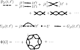
Figure 1: Feynman diagrams for the Cooper-pair fluctuations $\mathcal{D}_{jl}(t,t^{\prime})$ (bold dashed line) and the self-energy $\Sigma_{jl}(t,t^{\prime})$ in terms of the fully interacting Green’s functions (bold line). The last line shows an exemplary contribution to the Luttinger-Ward functional.

We use a self-consistent formulation of the diagrammatic equations, i.e., $\mathcal{D}$ and $\Sigma$ are expanded in terms of the fully interacting Green’s function. The self-energy functional $\Sigma[G]$ is then derivable from a Luttinger-Ward functional $\Phi[G]$, $\Sigma_{jl}(t,t^{\prime})=\delta\Phi[G]/\delta G_{lj}(t^{\prime},t)$ (see Fig. 1). This ensures energy and particle number conservation,Baym and Kadanoff (1961) which is particularly important to study the evolution of the total energy in the non-equilibrium dynamics. Interestingly it has also been found that the self-consistent expansion qualitatively well captures the normal state behavior of the correlation length in the two-dimensional system, which undergoes a Berezinsky-Kosterlitz-Thouless transition Engelbrecht and Nazarenko (2000) (see also Sec. III.1).

The attractive Hubbard model has also a sub-leading instability towards charge density wave order, which becomes degenerate with superconductivity at half filling. While there are predictions to manipulate the relative strength of the two orders in non-equilibrium, both by time-dependent protocolsSentef et al. (2017) and by electric currentsMatthies et al. (2018), the present formalism captures only the superconducting instability. To study the competition of short-range transient Cooper-pair and charge density wave correlations would definitely be interesting, but requires a different diagrammatic approach, which is left for future work.

II.3 Implementation

In real-space, the diagrammatic equations depicted in Fig. 1 read as follows. The pairing correlations satisfy the integral equation

$$\mathcal{D}_{jl}(t,t^{\prime})=\mathcal{D}^{0}_{jl}(t,t^{\prime})+\sum_{m}\int_{\mathcal{C}}\!\!d\bar{t}\,\,\mathcal{D}^{0}_{jm}(t,\bar{t})U(\bar{t})\mathcal{D}_{ml}(\bar{t},t^{\prime}),$$ (6)

where $\mathcal{D}^{0}_{jl}=iG_{jl}(t,t^{\prime})G_{jl}(t,t^{\prime})$ is the bare pairing correlation. The electronic self-energy is then given by

$$\Sigma_{jl}(t,t^{\prime})=-iV_{jl}(t,t^{\prime})G_{lj}(t^{\prime},t),$$ (7)

with $V_{jl}(t,t^{\prime})=U(t)\mathcal{D}_{jl}(t,t^{\prime})U(t^{\prime})$. All real-space functions depend only on space difference, and we solve the equations in momentum space on a finite momentum grid. After Fourier transform, Eq. (6) becomes

$$\mathcal{D}_{\bm{q}}(t,t^{\prime})=\mathcal{D}^{0}_{\bm{q}}(t,t^{\prime})+\int_{\mathcal{C}}\!d\bar{t}\,\,\mathcal{D}^{0}_{\bm{q}}(t,\bar{t})U(\bar{t})\mathcal{D}_{\bm{q}}(\bar{t},t^{\prime}),$$ (8)

with

$$\mathcal{D}^{0}_{\bm{q}}(t,t^{\prime})=\frac{i}{L^{2}}\sum_{\bm{k}}G_{\bm{k}}(t,t^{\prime})G_{\bm{q}-\bm{k}}(t,t^{\prime}).$$ (9)

The self-energy (7) in momentum space is given by

$$\Sigma_{\bm{k}}(t,t^{\prime})=\frac{-i}{L^{2}}\sum_{\bm{q}}V_{\bm{q}}(t,t^{\prime})G_{\bm{q}-\bm{k}}(t^{\prime},t),$$ (10)

with $V_{\bm{q}}(t,t^{\prime})=U(t)\mathcal{D}_{\bm{q}}(t,t^{\prime})U(t^{\prime})$. Finally, the momentum-dependent electronic Green’s functions satisfy the Dyson equation

$$G_{\bm{k}}(t,t^{\prime})=[i\partial_{t}-\epsilon(\bm{k},t)-\Sigma_{H}(t)-\Sigma_{\bm{k}}(t,t^{\prime})]^{-1},$$ (11)

with the Hartree self-energy $\Sigma_{H}(t)=U\langle n(t)\rangle$.

The numerical solution of Eqs. (8) to (11) is performed on a finite momentum grid of $L\times L$ points in the Brillouin zone. The number of independent $\bm{k}$-points depends on the symmetry of the problem. The latter is reduced in the presence of an external field, which is why simulations for nonzero field will be performed for smaller lattices. Equations (11) and (8) are integral equations on $\mathcal{C}$, which can be solved using high-order accurate algorithms for Volterra integral equations.Aoki et al. (2014); Eckstein et al. (2010) The main numerical bottleneck is the memory required to store the double-time functions $G_{\bm{k}}$ and $\mathcal{D}_{\bm{k}}$ at each $\bm{k}$. Equations (11) and (8) can be parallelized on several computing nodes, but the evaluation of the momentum sums in (10) and (9) then requires a collective communication.

II.4 Observables

In Sec. III below we analyze in particular the behavior of the pairing correlations in real space, which are obtained from the function (5) at equal time,

$$D(\bm{R}_{j}-\bm{R}_{l},t) \equiv\langle\hat{\Delta}_{l}^{\dagger}(t)\hat{\Delta}_{j}(t)\rangle=i\mathcal{D}^{<}_{jl}(t,t)$$ (12)

$$=\frac{1}{L^{2}}\sum_{\bm{q}}e^{i\bm{q}(\bm{R}_{j}-\bm{R}_{l})}i\mathcal{D}_{\bm{q}}^{<}(t,t).$$ (13)

Another important observable to be discussed is the total energy density, $E_{tot}(t)=\langle H(t)\rangle$. We have

$$E_{tot}(t) =E_{kin}+E_{int},$$ (14)

$$E_{kin}(t) =\frac{1}{L^{2}}\sum_{\bm{k},\sigma}\epsilon(\bm{k},t)n_{\bm{k},\sigma}(t)$$ (15)

$$E_{int}(t) =\frac{1}{L^{2}}\sum_{\bm{k}}(-i)[\Sigma_{\bm{k}}\ast G_{\bm{k}}]^{<}(t,t)$$ (16)

where $n_{\bm{k},\sigma}(t)=-iG_{\bm{k}}^{<}(t,t)$. In the second equation, the symbol $\ast$ denotes the convolution along $\mathcal{C}$, and Eq. (16) is obtained from the equation of motion for $G$. In the numerical implementation, we have confirmed that $E_{tot}(t)$ remains time-independent up to the numerical accuracy when $H(t)$ is time-independent (e.g., after an interaction quench), which must be the case because a conserving approximation is used for the self-energy.

III RESULTS

III.1 Equilibrium properties

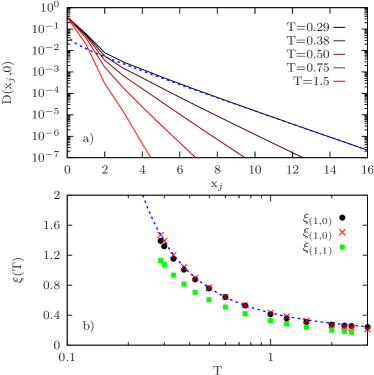
Figure 2: a) Pairing correlations $D(x_{j},0)$ along the $(1,0)$ direction of the lattice for interaction $U=-3$ and various temperatures $T$. $L=70$ is the lattice size. The dashed line shows a fit with Eq. (17) in the range $10\leq x_{j}\leq 30$. b) Correlation length $\xi(T)$ extracted from the fit of the data in panel a) with Eq. (17) in the range $10\leq x_{j}\leq 30$ (cross symbols) and $4\leq x_{j}\leq 8$ (circles). The line plots Eq. (18) with $A=1.275$ and $T_{\text{BKT}}=0.03$. Square symbols show the correlation length extracted from $D(x_{j},x_{j})$ along the $(1,1)$-direction.

Before studying the driven system, we briefly summarize the equilibrium properties of the model. Figure 2a shows the pairing correlations $D(\bm{R})$ [Eq. (12)] as a function of distance along the (1,0)-direction of the lattice, $D(x_{j},0)$. For all temperatures, we observe a decay at large distances, with an increase of the correlation length with decreasing temperature. In two dimensions, true long range order is not possible for $T>0$, but the system is expected to undergo a Berezinsky-Kosterlitz-Thouless (BKT) transition at some temperature $T_{\text{BKT}}$. In the normal phase, correlations asymptotically decay like

$$D(|\bm{R}|)\sim\frac{1}{|\bm{R}|^{1/4}}e^{-|\bm{R}|/\xi(T)},$$ (17)

with a temperature-dependent correlation length $\xi(T)$ which diverges at the BKT transition like

$$\xi(T)\sim\exp(A/\sqrt{T-T_{\text{BKT}}}).$$ (18)

We extract $\xi(T)$ from a fit to the numerical data in Fig. 2a with Eq. (17). The correlation length is shown in Fig. 2b, together with a fit (blue dashed curve) representing Eq. (18). Because the temperatures accessed in this investigation are considerably larger than $T_{\text{BKT}}$, fitting Eq. (18) does not give a very accurate value for $T_{\text{BKT}}$, although it has been noted that the critical region in the two-dimensional Hubbard model is relatively wide.Engelbrecht and Nazarenko (2000) In order to reach lower temperatures, one would have to study larger system sizes $L$ to ensure that $L\gg\xi(T)$. For the present analysis this turns out to be not necessary, because the correlation length reached in the driven states remains of the same order as in Fig. 2.

For later reference we also note that in the present regime the correlation length can be estimated already accurately from relatively short distances $4\leq x_{j}\leq 8$, see the black circles in Fig. 2b. Furthermore, although $\xi$ is only of the order of few lattice constants, the decay of correlations in space is already fairly isotropic, and the correlation lengths extracted along the $(1,0)$ and $(1,1)$-directions do not differ much (compare cross and square symbols in Fig. 2b).

III.2 Interaction ramp

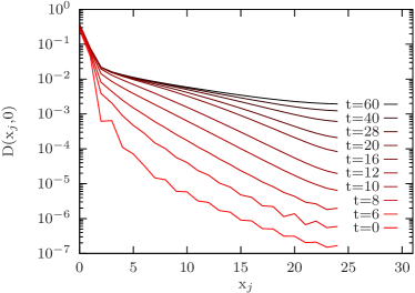
Figure 3: Pairing correlations $D(\bm{R})$ along the $(1,0)$-direction ($\bm{R}=(x_{j},0)$) for a ramp of interaction from $U_{i}=-0.5$ to $U_{f}=-3.0$, plotted at various times. (Lattice size $L=50$, initial temperature $T=1/15$).

Before analyzing the field-driven systems we study the build-up of pairing correlations in the Hubbard model after an artificial increase of the interaction. In this way the energy can change only during the ramp, and a controlled renormalization of the ratio $|U|$/bandwidth is obtained without energy absorption from a drive. We ramp the interaction between values $U_{i}$ and $U_{f}$ according to the protocol

$$U(t)=\begin{cases}U_{i}+(U_{f}-U_{i})\sin(\pi t/2t_{c})^{2}&\text{for }t\leq t_{c}\\ U_{f}&\text{for }t>t_{c}\\ \end{cases}.$$

The ramp duration $t_{c}=12$ is chosen slow enough such that the system remains close to adiabatic. (For a sudden quench ($t_{c}=0$) the system is strongly excited, so that pairing correlations simply decay with time).

In Fig. 3, we plot the pairing correlations $D(\bm{R})$ along the (1,0)-direction of the square lattice for a ramp $U_{i}=-0.5$ to $U_{f}=-3.0$. In the initial state the Cooper-pair correlations decay on the scale of few lattice sites. They start to grow in space during and after the pulse, and finally approach a steady regime. At intermediate times the behaviour of $D(\bm{R})$ signals the existence of two length scales. For example, the curve at $t=28$ has different slopes for $j\lesssim 15$ and $j\gtrsim 15$. This may be a signature of spreading correlations:Cheneau et al. (2012) For large distance, the correlations still maintain a fast decay like in the initial state, and a new correlation length can only be established in a range $|\bm{R}|<v_{D}t$ where $v_{D}$ is some maximal speed for the spread of the correlations. Estimating the velocity of the spreading of correlations from the point in space where $D$ takes a given value, e.g., $D(\hat{x}v_{D}t,t)=10^{-3}$, gives $v_{D}\approx t_{hop}$ at times $t$=12 around the end of the ramp. Although for a detailed systematic analysis the system size is not large enough, one can see that, as expected, the correlations spread slower than the electron velocity (the maximal group velocity of electrons, at $\bm{k}=(\pi/2,\pi/2)$, is $v_{max}=4t_{hop}$), but fast enough to extend over the system sizes studied below within the simulated time.

At long times, the correlations saturate at values much larger than in the initial state. This is because the effective temperature of the system after the slow ramp is comparable to the initial temperature of the system (see also next section), such that even after a thermalization of the system the correlation would not further decay. A behavior as observed in the DMFT simulations for the anti-ferromagnetic order,Bauer et al. (2015) where after the ramp the system undergoes a transient regime with increased correlation length before thermalization, is found for shorter ramp time. In this case however, the system is strongly excited, and also the transient increase of the correlation length is relatively small.

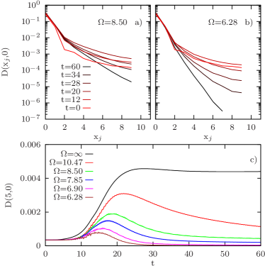
Figure 4: Pairing correlations $D(\bm{R})$ along the $(1,0)$-direction for various times in the field-driven system. The driving frequency is $\Omega=8.50$ for (a) and $\Omega=6.28$ for (b). Both simulations are for $U/t_{hop}=-1$, and $U/t_{\text{hop}}^{\text{eff}}=-3$ after ramp-on of the time-periodic driving. (Lattice size $L=20$, initial temperature $1/15$.) c) $D(\bm{R})$ at $\bm{R}=(5,0)$ as a function of time, for various driving frequencies $\Omega$.

III.3 Floquet band renormalization

We now proceed to analyze the dynamics induced by an oscillating electric field. We choose the vector potential in Eq. (3) with projection $A(t)=A_{0}(t)\cos(\Omega t)$ along (1,1)-direction. A smaller lattice size ($L=20$) is consider for the field-driven simulations, because the reduced lattice symmetries in the driven case requires more momentum points (see Sec. II). Within a time $t_{c}$ the amplitude $A_{0}(t)$ is ramped up to a final vale $A_{f}$ (correspondingly the amplitude of the electric field is $E_{0}=A_{f}\Omega$), with a ramp profile $A_{0}(t)=(t/t_{c})^{2}A_{f}$ for $t<t_{c}$ and $A_{0}(t)=A_{f}$ for $t>t_{c}$. We choose $A_{f}=1.8114$, such that after the ramp the effective hopping is reduced by a factor $t_{\text{hop}}^{\text{eff}}/t_{\text{hop}}=\mathcal{J}_{0}(A_{f})=1/3$ [c.f. Eq. (1)], and the ratio $|U|$/bandwidth is increased by a factor three. In the following, we will refer to the attractive Hubbard (2) model with $U=-1$ and $t_{\text{hop}}=1/3$ simply as the “effective Hamiltonian”, and compare the properties of the driven system with the equilibrium properties of the latter.

Figure 4a and b show the emerging pairing correlations for various times and driving frequencies $\Omega=8.50$ and $\Omega=6.28$ slightly above and below the non-interacting bandwidth $W=8t_{\text{hop}}$. For the earlier times, we observe an increase of the correlations similar to the behavior after the interaction ramp [Fig. 3], but i the driven system pair correlations steadily decrease at later times. The non-monotonous evolution is illustrated by the time-dependence of $D(\bm{R})$ at a given point $\bm{R}=(5,0)$, see Fig. 4c. Only for $\Omega=\infty$, which is simulated as a time-dependent ramp of the hopping amplitude given by $t_{\text{hop}}^{\text{eff}}(t)=t_{\text{hop}}\mathcal{J}_{0}(A_{0}(t))$, one observes an increase which prevails towards long times. The analysis shows that with realistic pulses frequencies close to the bandwidth one can achieve a significant enhancement of the superconducting correlations, in spite of the energy absorption which, as we will see now, is the reason for the suppression of the order at longer times.

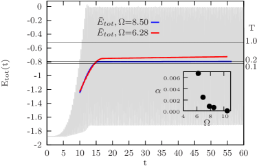
Figure 5: Time-dependent energy $E_{tot}(t)$ of the driven system [c.f. Eq. (14)]: The black and red lines give the moving average of the energy over $10$ periods, for driving frequencies $\Omega=8.50$ and $6.28$ within and outside the bandwidth. The full oscillations of $E_{tot}$ are indicated by the light grey lines for $\Omega=10.47$; the amplitude of the oscillations is similar in magnitude for other frequencies. The labels at the right vertical axis show the temperature of an un-driven system in equilibrium with renormalized hopping $t_{\text{hop}}=1/3$ and an energy density corresponding to the left vertical axis. Inset: Energy absorption of the system for different driving frequencies after the ramp.

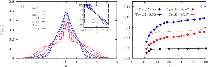
Figure 6: (a) The local spectral function for a driving frequency $\Omega=10.47$ at different times. Oscillations on the spectra at early times are due to finite cut-off of the Fourier integral in Eq. (19). Inset: The ratio $\kappa(\omega,t)=\ln\Big{[}\frac{A^{<}(\omega,t)}{A^{>}(\omega,t)}\Big{]}$ for the same driving frequency. (b) Temperature $T_{\text{FS}}$ [Eq. (20)] for different driving frequencies.

In order to test to what extent the decrease of the pairing correlations at long time is explained by the energy absorption, we evaluate the total energy $E_{tot}(t)$ [Eq. (14)], and compare to the energy of the effective Hamiltonian at different temperatures (Fig. 5). It is important to note that the time-dependence of $E_{tot}$ (light grey line in Fig. 5), or the instantaneous value $E_{tot}(t)$ itself tells nothing about the energy absorption. During one cycle, $E_{tot}$ falls well below the ground state energy of the effective Hamiltonian, so that this value cannot be related to an “effective temperature” of the latter. The energy absorption becomes instead manifest in the energy $\bar{E}_{tot}(t)=\frac{1}{\tau}\int_{t-\tau/2}^{t+\tau/2}d\bar{t}\,E_{tot}(\bar{t})$ averaged over few periods, $\tau=n2\pi/\Omega$: The latter shows a linear increase $\bar{E}_{tot}(t)\sim\alpha t+\text{const.}$ after the ramp, with a threshold-like increase of the rate $\alpha(\Omega)$ for frequencies $\Omega\approx 8t_{\text{hop}}$ around the bandwidth (inset of Fig. 5).

It is now a natural question whether the effective temperature estimate from the mean energy $\bar{E}_{tot}$ can explain the build-up and decay of the superconducting correlations. Below we will see that this is not the case: The Floquet system in equilibrium with the same energy density $\bar{E}_{tot}$ as the driven system would have lower superconducting correlations. A different temperature estimate can be obtained from the electronic distribution functions. In equilibrium, the fluctuation-dissipation theorem (FDT) for fermions gives a universal ratio between the occupied density of states $A^{<}(\omega)$ and the spectrum $A^{<}(\omega)=f(\omega)A(\omega)$. Here $A(\omega)=-\frac{1}{\pi}\text{Im}G^{R}(\omega)$, and $A^{<}(\omega)=\frac{1}{2\pi i}G^{<}(\omega)$, where $G^{<}(t,t^{\prime})=i\langle c(t^{\prime})^{\dagger}c(t)\rangle$ and $G^{R}(t,t^{\prime})=-i\theta(t-t^{\prime})\langle\{c(t),c(t^{\prime})^{\dagger}\}\rangle$ are the lesser and retarded propagators respectively, and $f(\omega)$ is the Fermi function. In the driven case, we evaluate time-dependent spectra, and similar $A^{<}$, as

$$A(t,\omega)=-\frac{1}{\pi}{\rm{Im}}\int^{t_{cut}}_{0}dse^{i\omega s}G^{R}(t+s,t),$$ (19)

with $t_{cut}=30$, averaged over few driving periods (for later times an analogous backward Fourier transform is used). A convenient quantity to verify the FDT is the logarithmic ratio $-\ln\big{[}A(\omega)/A^{<}(\omega)-1]\equiv\ln\big{[}A^{<}(\omega)/A^{>}(\omega)]$, which gives a linear function $\kappa(\omega)=-\omega/T$ in a thermal equilibrium state. In Fig. 6a, we plot the time-dependent local spectra and the ratio $\kappa(\omega,t)\equiv\ln\Big{[}\frac{A^{<}(\omega,t)}{A^{>}(\omega,t)}\Big{]}$ for $\Omega=10.47$. One can see that $\kappa(\omega,t)$ is linear around $\omega=0$, which represents the energy range of electrons close to the Fermi surface, while away from the Fermi surface the distribution functions take a more non-thermal form. We therefore extract an effective temperature $T_{\text{FS}}(t)$ of the electrons at the Fermi surface as

$$\frac{1}{T_{\text{FS}}(t)}=-\frac{d}{d\omega}\ln\Big{(}\frac{A^{<}(\omega,t)}{A^{>}(\omega,t)}\Big{)}_{\omega=0},$$ (20)

This temperature turns out to be consistently lower than the temperature obtained from the average energy (Fig. 6b): For $\Omega=8.50$ and $t=60$, e.g., the energy density $\bar{E}_{tot}(t)$ corresponds to a temperature $T=0.192$ in the effective Hamiltonian system [Fig. 5], while $T_{\text{FS}}=0.117$. This indicates that the driven system is in a strongly non-thermal state, in which different energy regions are not yet thermalized, so that a description by a single effective temperature of the Floquet system is not possible.

We can now investigate which temperature is suited to estimate the superconducting correlations. In Fig. 7 we plot the correlation length $\xi(t)$ of the Floquet system ($U=-1$, $t_{\text{hop}}=1/3$) as function of temperature (up to a rescaling, this is the same as Fig. 2b). In addition, we extract the correlation length $\xi(t)$ from the driven system (Fig. 4) at different times, and plot the result against the low-energy temperature $T_{\text{FS}}(t)$ (filled circles). One can see that the Cooper-pair correlations in the driven state follow more closely the equilibrium behavior set by the effective temperature of the electrons at the Fermi surface, while the correlation length at the temperature estimate from the mean energy would be considerably shorter.

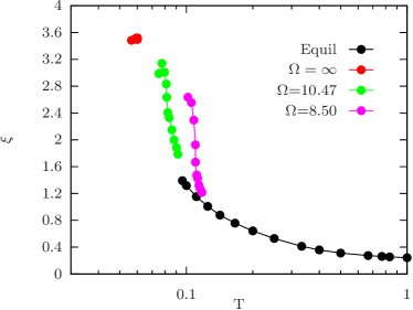
Figure 7: Correlation length $\xi$ of the driven system, extracted from a fit with Eq. (17) to the time-dependent data in the range $4\leq x_{j}\leq 8$. Black circles: Correlation length for the effective Hamiltonian system ($U=-1$, $t_{\text{hop}}=-1$).

Finally, we remark that similar to the electronic temperature, one can also extract a temperature of the bosonic fluctuations, as $T_{D}^{-1}=-\frac{d}{d\omega}[\mathcal{D}^{<}(\omega,t)/\mathcal{D}^{>}(\omega,t)]_{\omega=0}$, in analogy to Eq. (20). This temperature is comparable in magnitude to $T_{\text{FS}}$ (see dashed line in Fig. 6b).

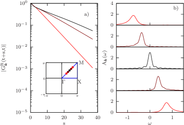
Figure 8: (a) The modulus of the retarded Green’s function at time $t$=23 for values of $\bm{k}$ along the $\Gamma$-$M$ direction of the Brillouin zone($\Omega=10.47$). Inset: The corresponding $\bm{k}$ points in the Brillouin zone. (b) Momentum resolved spectral function as a function of frequency for the same momentum.

III.4 Electronic spectra

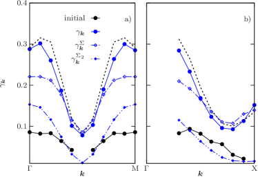
Figure 9: (a) Relaxation rate obtained from the real-time data Eq. (21) (circles, $\gamma_{\bm{k}}$), from the self-energy [c.f. Eq. (23)] (open squares, $\gamma_{\bm{k}}^{\Sigma}$), and from the second-order self-energy (filled squares, $\gamma_{\bm{k}}^{\Sigma_{2}}$), for values of $\bm{k}$ along the $\Gamma$-$M$ direction in the Brillouin zone at time $t=23$ after the ramp ($\Omega=10.47$). The dashed line shows $\gamma_{\bm{k}}$ for the effective Hamiltonian ($t_{\text{hop}}$=1/3, $U=-1$) in equilibrium at temperature $T=T_{\text{FS}}=0.10$. (b) Relaxation rate $\gamma_{\bm{k}}$ for momenta $\bm{k}$ along the $\Gamma$-$X$ direction, $X=(0,\pi)$.

Superconducting fluctuations in the normal state can have a strong effect on the electronic spectra. They can give rise to a pseudo-gap behaviour, and for ramps close to the superconducting transition an anomalous increase of the quasi-particle lifetime close to the Fermi-surface has been predicted. Lemonik and Mitra (2017) For the parameters investigated here, there is no pseudo-gap in the local density of states (see Fig. 6a). This is not un-expected, as the effective temperature (both $T_{\text{FS}}$ and the estimate from the global energy density) is too high for a pseudo-gap to appear even in an equilibrated system. For a more detailed comparison of the electronic spectra of the effective Hamiltonian ($t_{\text{hop}}=1/3$ and $U=-1$) and the driven system we therefore analyze the momentum-dependent Green’s functions $G_{\bm{k}}$ and the Fermi-liquid properties of the system.

In a Fermi-liquid, the momentum dependent retarded Green’s function in time has the asymptotic quasi-particle form

$$G_{\bm{k}}^{R}(t)\sim G_{\bm{k}}^{coh}(t)\equiv-iZ_{\bm{k}}e^{-i{\tilde{\epsilon}}_{\bm{k}}t}e^{-\gamma_{\bm{k}}t}$$ (21)

where ${\tilde{\epsilon}}_{\bm{k}}$ is the quasi-particle energy, and $\gamma_{\bm{k}}$ the relaxation rate. One can therefore directly extract $\gamma_{\bm{k}}$ from the real-time data: In Fig. 8a, we exemplarily show $|G^{R}_{\bm{k}}(t+s,t)|$ at time $t=23$ for values of $\bm{k}$ along the $\Gamma$-$M$ direction of the Brillouin zone. The functions decay exponentially at long times ($s$), from which $\gamma_{\bm{k}}$ is extracted. This procedure is equivalent of measuring the Lorentzian line-width of the momentum-resolved spectra $A_{\bm{k}}(\omega,t)$. Just for illustration, we plot in Fig. 8b the spectra $A_{\bm{k}}(\omega,t)$, obtained from the Fourier transforms of the real time data $G^{R}_{\bm{k}}(t+s,t)$ using Eq. (19).

Figure 9a shows $\gamma_{\bm{k}}$ along the $\Gamma$-$M$ direction of the Brillouin zone for different times. The electron relaxation rate is consistent with the finite-temperature Fermi liquid form

$$\gamma_{\bm{k}}\sim C{|\bm{k}-\bm{k}_{F}|}^{2}+C^{\prime},$$ (22)

but shows a marked increase at $\bm{k}=\bm{k}_{F}$ compared to the initial state. In analogy to the superconducting fluctuations, we find that the relaxation rates match fairly well the behavior of the effective Hamiltonian system in equilibrium at temperature $T_{\text{FS}}$ (see dashed lines). Consistent with this observation, we now show that the increase of $\gamma_{\bm{k}_{F}}$ with respect to the initial state can largely be assigned to the coupling of electrons and Cooper-pair fluctuations.

The effect of the Cooper-pair correlations on the electronic spectra can be quantified as follows: We first confirm that the lifetime of the quasiparticles can also be obtained from the self-energy. The estimate

$$\gamma_{\bm{k}}^{\Sigma}=-\text{Im}\Sigma^{R}(\omega=\tilde{\epsilon}_{\bm{k}},t),$$ (23)

measured at some time $t$ in the driven state, accurately reproduces $\gamma_{\bm{k}}$ from the real-time data, compare circles and open squares in Fig. 9a. (To first approximation, $\tilde{\epsilon}_{\bm{k}}$ in Eq. (23) is taken as the bare band energy $\mathcal{J}_{0}(A_{f})\epsilon_{\bm{k}}=\epsilon_{\bm{k}}/3$, since we are anyway mainly interested in the properties at the Fermi surface $\epsilon_{\bm{k}}=0$.) Furthermore, we can then obtain the contribution $\gamma_{\bm{k}}^{\Sigma_{2}}$, by taking only the second-order self-energy $\Sigma_{\bm{k}}^{(2)}$ in Eq. (23), which does not take into account the Cooper-pair correlations. (To obtain $\Sigma_{\bm{k}}^{(2)}$, the full propagator $\mathcal{D}$ in Eq. (10) is replaced by Eq. (9). Note that this is only a decomposition of the different contributions to $\Sigma$; the driven state is always evaluated with the full self-energy). From the comparison of the relaxation rates $\gamma_{\bm{k}}^{\Sigma_{2}}$ and $\gamma_{\bm{k}}^{\Sigma}$, we see that the increase of the scattering rate at the Fermi surface in the driven state can be attributed mainly to the interaction with the Cooper-pair fluctuations. This observation is consistent with Ref. Lemonik and Mitra, 2017, where the build-up of superconducting fluctuations lead to an anomalous peak of the scattering rate at the Fermi energy for a system that was quenched right to the superconducting transition. In the present case, however, the impact of the fluctuations on the scattering rate is rather featureless, as the driven system is at a higher effective temperature and further from a phase transition, so that the superconducting correlations extent only over few lattice constants.

The increase of the scattering rate in the driven state compared to the initial state is also visible along the $\Gamma-X$ direction (Fig. 9b). Interestingly, in this case there is a pronounced peak in the scattering rate at $\bm{k}=X$. This anomalous behavior is actually not exclusively due to the pairing fluctuations. Although small on the scale of Fig. 9b, it can already be seen in the scattering rate $\gamma^{\Sigma_{2}}_{\bm{k}}$ obtained from the (filled squares), and also in the $\gamma^{\Sigma_{2}}_{\bm{k}}$ in equilibrium at temperatures $T>0$ (not shown). The enhanced scattering is simply a consequence of the flat dispersion $\epsilon_{\bm{k}}$ at $\bm{k}=X$, which is the origin of the van-Hove singularity in the density of state at $\omega=0$. However, as one can see from the comparison of $\gamma^{\Sigma}_{\bm{k}}$ and $\gamma^{\Sigma_{2}}_{\bm{k}}$, the effect is greatly enhanced by the coupling of electrons and superconducting fluctuations. The latter suggests the interesting experimental possibility of exploiting the van-Hove points to amplify the signature of the fluctuations in the electronic spectra. In the present case, the van-Hove point accidentally lies on the Fermi-surface, but in general one can think of deforming the band structure through Floquet engineering in such a way that a van-Hove point is shifted to the Fermi surface. While this will typically require strong fields, such that an enhancement of electronic orders is possibly only transiently, our simulation suggests that at such a van-Hove point even the short range fluctuations reachable in a transient Floquet engineering protocol can become evident, making this an experimentally viable pathway.

IV Conclusion

In conclusion, we have studied the dynamical enhancement of short-range superconducting fluctuations in the attractive Hubbard model following a renormalization of the bandwidth by a time-periodic electric field with frequencies close to the bandwidth. In the effective (Floquet) Hamiltonian picture, which is asymptotically correct in the limit of large driving frequency, the driving corresponds to a reduction of the hopping matrix elements, and hence an increase of the ratio interaction over bandwidth. At finite frequency, the system constantly absorbs energy from the drive and therefore does not reach a long-range ordered state in the long-time limit. Instead, short range correlations increase at short times, and decrease as the system subsequently heats up. Based on numerical simulations, our main observations are the following: (i) Even with driving frequencies close to the bandwidth, a substantial enhancement of the short-range superconducting fluctuations can be achieved at least transiently. (ii) The driven state at intermediate times is rather non-thermal. It cannot be described by an effective temperature state of the effective Hamiltonian, and a temperature estimate $T_{\text{FS}}$ from the electrons close to the Fermi surface is still lower than an estimate based on the global energy in the system. Superconducting fluctuations in the transient state are determined more accurately by the effective temperature $T_{\text{FS}}$ and are thus more “robust” against the energy absorption. (iii) The superconducting fluctuations lead to an increase of the electronic quasiparticle scattering rate. While for the short-ranged correlations this increase is in general rather featureless over the Brillouin zone, the effect of short-range fluctuations is strongly enhanced at a van-Hove point in the band structure.

Although it is clearly challenging to use Floquet engineering as a way to induce long-range orders out of a gapless metallic state, our work demonstrates that the manipulation of short-range orders is in range experimentally, with frequencies that do not have to be far detuned from the bandwidth. Using the amplifying effect of van-Hove singularities, it may be possible to observe such a transient Floquet control of electronic orders. (Furthermore, indirect signatures of short-range superconducting correlations have been predicted in the optical conductivity.Ido et al. (2017); Bittner et al. (2017); Lemonik and Mitra (2018)) An interesting pathway for further investigations is also the control of (short range) charge order, which can be monitored more directly using time-resolved X-rays from free electron lasers. Charge-ordered systems (or systems where charge-order and superconductivity are intertwined) are also more strongly coupled to the lattice, which may eventually even stabilize different driven states at longer time.