Spin-orbit Interactions for Singlet-Triplet Qubits in Silicon

Abstract

Spin-orbit coupling is relatively weak for electrons in bulk silicon, but enhanced interactions are reported in nanostructures such as the quantum dots used for spin qubits. These interactions have been attributed to various dissimilar interface effects, including disorder or broken crystal symmetries. In this Letter, we use a double-quantum-dot qubit to probe these interactions by comparing the spins of separated singlet-triplet electron pairs. We observe both intravalley and intervalley mechanisms, each dominant for [110] and [100] magnetic field orientations, respectively, that are consistent with a broken crystal symmetry model. We also observe a third spin-flip mechanism caused by tunneling between the quantum dots. This improved understanding is important for qubit uniformity, spin control and decoherence, and two-qubit gates.

I Introduction

Isotopically enriched silicon is a prime semiconductor for the implementation of spin qubits Loss and DiVincenzo (1998). In addition to reduced spin decoherence enabled by the near absence of lattice nuclear spins Witzel et al. (2010); Veldhorst et al. (2014), silicon is a low spin-orbit coupling material for electrons that enables long spin relaxation times Zwanenburg et al. (2013); Watson et al. (2017) and low coupling to charge noise. In silicon quantum dots (QDs), recent work has shown that spin-orbit effects arise in the presence of strong electron confinement Yang et al. (2013); Veldhorst et al. (2015); Eng et al. (2015); Ferdous et al. (2018); Jock et al. (2018); Corna et al. (2018). This enhanced interaction has been attributed to intervalley spin-orbit coupling and interface disorder Yang et al. (2013); Veldhorst et al. (2015); Corna et al. (2018) in some works, and to broken crystal symmetries Rössler and Kainz (2002) at the Si/SiO₂ Jock et al. (2018) or Si/SiGe Prada et al. (2011) interfaces in other works. Recently, Jock et al. (2018) have used a singlet-triplet (ST) qubit Levy (2002); Petta et al. (2005) to probe the electron $g$-factor difference between two QDs, and found a strong magnetic-field-dependent anisotropy explained with an intravalley mechanism. This anisotropy can be exploited to enhance spin-orbit effects for spin control Veldhorst et al. (2014); Jock et al. (2018), or suppress them for uniformity and reproducibility Li et al. (2018). ST qubits are promising candidates for quantum computing, thanks to the ability to perform exchange Levy (2002), capacitive Shulman et al. (2012); Srinivasa and Taylor (2015); Nichol et al. (2017), and long-range Trifunovic et al. (2012); Mehl et al. (2014); Srinivasa et al. (2015); Malinowski et al. (2018) two-qubit gates, as well as low-frequency one-qubit operations Taylor et al. (2007). In GaAs devices, the use of differential dynamic nuclear polarization (DDNP) was shown to dramatically enhance the ST qubit coherence Bluhm et al. (2010); Shulman et al. (2014), and also enable its control Foletti et al. (2009); Shulman et al. (2014). The DDNP technique depends on the interaction between the two-electron spin singlet $\left|S\right>=(\left|\uparrow\downarrow\right>-\left|\downarrow\uparrow\right>)/\sqrt{2}$ and spin triplet $\left|T_{-}\right>=\left|\downarrow\downarrow\right>$ mediated by the hyperfine coupling to lattice nuclear spins Gullans et al. (2010). It was shown that spin-orbit interaction can couple these two states as well Stepanenko et al. (2012), impacting the ability to perform a DDNP by providing an alternate channel to dissipate angular momentum Rančić and Burkard (2014); Nichol et al. (2015). In light of these different works, it remains unclear what spin-orbit effects predominate in different situations, what their microscopic origins are, and how these effects will impact the operation of silicon devices.

In this Letter, we report the observation of three different spin-orbit effects in the same device using a ST qubit in isotopically enriched silicon. The first two effects are probed using $S{-}T_{0}$ precession and appear at different orders of perturbation theory. They consist of an intravalley $g$-factor difference effect and an intervalley spin-coupling effect. The dominant mechanism depends on the magnetic field orientation with respect to crystallographic axes. We report here a nonlinear magnetic field strength dependence, in addition to previously reported linear dependences. The third effect is probed using $S{-}T_{-}$ spin transitions and involves a spin-flip process triggered by electron tunneling between the QDs. To measure this effect, we adapt a method previously used in GaAs Nichol et al. (2015) to our silicon system, where the near absence of nuclear spins otherwise prevents these transitions. We find that the enhanced spin-orbit interaction in the device strongly couples these states, as it does for GaAs devices. In fact, the spin-orbit length estimated from our measurements is only slightly smaller than bulk GaAs values, a result that is in accordance with other recent observations of strong spin-orbit effects in silicon nanodevices. This prevents us from performing DDNP of the residual ²⁹Si.

The effects are modeled with an analytical microscopic intravalley theory based on broken crystal symmetries introduced in Jock et al. (2018) and extended in this Letter to describe the additional intervalley effect reported here. The model involves the electron momentum only at the Si–SiO₂ interface, resulting in stronger-than-bulk first-order effects in the electron momentum and clear predictions that could help elucidate the microscopic origin of the enhanced spin-orbit effects in the future Ruskov et al. (2018). This Letter, as a consequence of its comprehensive view of spin orbit interactions, will affect how pulses are shaped around the uncovered transitions in silicon qubits as well as providing more detailed guidance about the implications of how samples are mounted in dilution refrigerators with respect to magnetic fields.

II Methods

The experiments are performed in a dilution refrigerator with an electronic temperature of around $300\text{ mK}$. The gated silicon QD device is shown in Fig. 1. The silicon is isotopically enriched ²⁸Si, with a measured $685\text{ ppm}$ of residual ²⁹Si. Fabrication and device crystallographic orientation are as in Jock et al. (2018); the device is from the same fabrication run but a different die and measured in a different system. Two QDs are formed, one under the bottom source (BS) gate and one under the bottom center (BC) gate. The bottom left (BL) and BC gates are used for fast control of the left (L) and center (C) QD charge occupations $(N_{\text{L}},N_{\text{C}})$ and interdot detuning $\epsilon$.

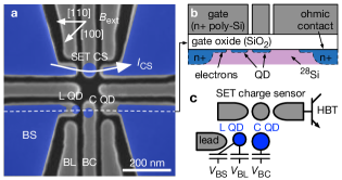
Figure 1: (a) Scanning electron microscope image of the gate structure of the silicon QD device. The blue overlay indicates the estimated locations of electron accumulation. The crystallographic and external magnetic field ($B_{\text{ext}}$) orientations are indicated. All experiments are performed with the magnetic field along the [100] orientation, except when otherwise specified. A SET CS is used for readout and sensing. Its current $I_{\text{CS}}$ is amplified using a SiGe HBT. (b) Schematic lateral view of the device structure (along the dashed line). (c) Conceptual view of the two QDs, the single-lead reservoir, the CS and the predominant QD-gate capacitive couplings. The BL and BC gates are used for fast electrical control of the L and C QDs, respectively.

The double QD is biased in a two-electron charge configuration to form a ST qubit. The L QD has a ST splitting of $243\text{ }\upmu\text{eV}$ and the C QD has one of $185\text{ }\upmu\text{eV}$ (the latter measured in a $(3,2)$ configuration to avoid charge latching). Spin readout is performed with a direct enhanced latching readout, as described in Harvey-Collard et al. (2018), and using a single-electron transistor (SET) in series with a SiGe heterojunction bipolar transistor (HBT) cryoamplifier Curry et al. (2015). Triplet return probabilities $P(T)$ are calculated from the average of readout traces referenced to a known charge configuration to eliminate the slow charge sensor (CS) current fluctuations.

The external magnetic field $B_{\text{ext}}$ is applied in-plane along the [100] or [110] crystallographic orientations. The [100] orientation is used for all the experiments unless otherwise specified. The [110] orientation was obtained by rotating the sample in a separate cooldown. The device parameters (voltages, ST splittings, etc.) remained very similar between cooldowns, except for slight changes in the tunnel couplings.

III Results

A charge stability diagram of the two-electron double QD and the typical location of the pulse sequence steps are shown in Fig. 2. We use rotations between the $\left|S\right>$ and $\left|T_{0}\right>=(\left|\uparrow\downarrow\right>+\left|\downarrow\uparrow\right>)/\sqrt{2}$ states to measure the difference in Zeeman energy perpendicular to the quantization axis $\Delta E_{z}$ between the two QDs. These rotations appear with the application of an external magnetic field $B_{\text{ext}}$, as reported in Jock et al. (2018), in spite of the (relative) absence of lattice nuclear spins or magnetic materials. The inhomogeneous dephasing time saturates at $T_{2}^{\star}=3.4\pm 0.3\text{ }\upmu\text{s}$ after 2 h of data averaging. This value is consistent with magnetic noise from residual ²⁹Si hyperfine coupling with the electron spins, and with other reported values Witzel et al. (2010); Assali et al. (2011); Eng et al. (2015); Rudolph et al. (2016); Jock et al. (2018).

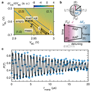
Figure 2: (a) Charge stability diagram of the two-electron double QD. The typical pulse sequence steps are indicated. They consist of an emptying step (empty) where the charge occupancy is reset and the current referenced, a load step (load) for singlet or mixture preparation, a transient point (roll) to set the pulse trajectories and rates, some steps in $(1,1)$ (points Z and J) for spin control, a return to “roll” step, and an enhanced latching readout step (meas.). The roll point can be placed on either sides of the $S{-}T_{-}$ anticrossing depending on the goals. More details about the pulses can be found in the Supplemental Material Sec. S1 and Sec. S2. (b) ST qubit Bloch sphere and pulse sequence for $S{-}T_{0}$ rotations. (c) Rotations between the $\left|S\right>$ and $\left|T_{0}\right>$ states versus the manipulation time $t_{\text{manip}}$. Those are enabled by a large $B_{\text{ext}}=1\text{ T}$ in the [100] direction, in spite of the relative absence of nuclear spins or magnetic materials. Optimal visibility is achieved in the rapid adiabatic passage (RAP) regime Taylor et al. (2007); Harvey-Collard et al. (2017) (see the Supplemental Material Sec. S1). The visibility is $73\text{\%}$, limited largely by preparation and readout errors. The dephasing time is $15\text{ }\upmu\text{s}$ for this single trace acquired in 4 minutes.

To investigate the physical origin of the $S{-}T_{0}$ rotations, we vary the strength of $B_{\text{ext}}$ along two orientations measured in successive cooldowns. We identify different dominant spin-orbit mechanisms for these two orientations, with the results summarized in Fig. 3.

Figure 3: (a) The three different spin-orbit effects for electrons in a silicon MOS nanodevice identified in this Letter. First, spin-orbit interaction in each dot leads to a renormalization of their effective $g$-factors. This entails an interaction of the form $\Delta E_{z}=\Delta g\mu_{\text{B}}B_{\text{ext}}$ (see Fig. 2b). Second, intervalley spin coupling can change the Landé factor $g^{*}$ of one dot in particular, leading to an interaction of the form $\Delta E_{z}\propto B_{\text{ext}}^{2}/\left(E_{\text{VS}}-g\mu_{\text{B}}B_{\text{ext}}\right)$. Third, electron motion during a tunneling event can induce a spin flip that couples the $(2,0)S$ and $(1,1)T_{-}$ states, as shown also in Fig. 4. (b) Fast Fourier transform (FFT) power of the $S{-}T_{0}$ rotations versus $B_{\text{ext}}$. For the [110] field orientation, the linear interdot effect dominates. For the [100] orientation, the linear interdot effect is suppressed; however, a second-order effect consistent with an intervalley mechanism is observed. The solid lines are fit to a complete Hamiltonian model detailed in the Supplemental Material Sec. S6 and agree well with the simple analytical forms described above. (c) The intervalley spin coupling in one of the dots perturbs the $S{-}T_{0}$ energy difference at the second order through the excited valley $\left|T_{-}^{*}\right>$ state. This simple model neglects the excited valley state of the other dot, which is higher in energy.

Figure 4: (a) Anticrossing of the $\left|S\right>$ and $\left|T_{-}\right>$ states. The separation $E_{\text{Z}}=g\mu_{\text{B}}B$ between the $(1,1)S$ and $(1,1)T_{-}$ states is tuned with the magnetic field $B$. The coupling strength $\varDelta_{\text{ST}}$ can come from both a tunneling plus spin-flip mechanism that couples $(1,1)$ and $(2,0)$ states, and from the hyperfine interaction with lattice nuclear spins which couples $(1,1)$ states together. For our residual ²⁹Si concentration, the latter should be less than $0.6\text{ neV}$ Witzel et al. (2010); Assali et al. (2011). (b) Pulse sequence for the spin funnel measurement. When the detuning pulse falls on the transition, mixing between $\left|S\right>$ and $\left|T_{-}\right>$ occurs. (c) Spin funnel with $t_{\text{wait}}=20\text{ }\upmu\text{s}$. This measurement allows us to calibrate the tunnel coupling $t_{\text{c}}$ and energy ramp rate $\mathrm{d}E/\mathrm{d}t$ of LZ sweeps. (d) Pulse sequence to probe the $S{-}T_{-}$ gap through LZ transition probabilities. (e) The magnetic field dependence of the gap is fit to a simple model that includes a constant spin-orbit term $\varOmega_{\text{SO}}$ and charge hybridization, see the Supplemental Material Eq. (S2). The confidence interval is explained in the Supplemental Material Sec. S3. The field is in the [100] direction.

The first mechanism is a first-order intravalley effect observed both in this device and in Jock et al. (2018). The Zeeman drive is a difference in effective Landé $g$-factor $\Delta g$ between the two QDs:

$$\Delta E_{z}=\Delta g\mu_{\text{B}}B_{\text{ext}}.$$ (1)

This effect dominates in the [110] field orientation. It is not predicted to depend on the double QD orientation, as shown by the different positions for the two QDs in this Letter compared with Jock et al. (2018).

The second mechanism, newly reported here, is consistent with an intervalley spin-orbit interaction Yang et al. (2013); Hao et al. (2014); Corna et al. (2018). The smaller and nonlinear behavior versus magnetic field from Fig. 3(b) suggests a second-order interaction with an excited valley $\left|T_{-}^{*}\right>$ state, as shown in Fig. 3(c). For simplicity, we consider only the QD with the lowest valley splitting $E_{\text{VS}}$. In the other QD, this interaction is suppressed by the larger $E_{\text{VS}}$. Using perturbation theory, we have

$$E_{S}-E_{T_{0}}=\left(E_{S}^{(0)}-E_{T_{0}}^{(0)}\right)+\ldots\\ \left(\frac{\left|\big{\langle}T_{-}^{*(0)}\big{|}{H_{\text{SO}}}\big{|}S^{(0)}\big{\rangle}\right|^{2}}{E_{S}^{(0)}-E_{T_{-}^{*}}^{(0)}}-\frac{\left|\big{\langle}T_{-}^{*(0)}\big{|}{H_{\text{SO}}}\big{|}{T_{0}}^{(0)}\big{\rangle}\right|^{2}}{E_{T_{0}}^{(0)}-E_{T_{-}^{*}}^{(0)}}\right).$$ (2)

Here, $E_{\psi}^{(i)}$ is the energy of the state $\left|\psi\right>$ at the $i^{\text{th}}$ order, and $H_{\text{SO}}$ is the spin-orbit interaction Hamiltonian. We note that the first term on the right-hand side is the effect of Eq. (1). This first term is largely suppressed for the [100] field orientation, as in Jock et al. (2018). The second term on the right-hand side can be simplified as follows. The matrix elements $\big{\langle}T_{-}^{*(0)}\big{|}{H_{\text{SO}}}\big{|}S^{(0)}\big{\rangle}$ and $\big{\langle}T_{-}^{*(0)}\big{|}{H_{\text{SO}}}\big{|}{T_{0}}^{(0)}\big{\rangle}$ are both proportional to $B_{\text{ext}}$, as explained in the Supplemental Material Sec. S6. Therefore, Eq. (2) simplifies to

$$\Delta E_{z}=\frac{\bar{\beta}_{C}^{2}B_{\text{ext}}^{2}}{2(E_{\text{VS}}-g\mu_{\text{B}}B_{\text{ext}})}.$$ (3)

Here, $\bar{\beta}_{C}$ is a measure of the Dresselhaus spin coupling of the C QD. The above treatment is simplistic but provides intuition about the physical mechanism and agrees well with the more detailed analysis of the Supplemental Material Sec. S6. We extract a value of $\bar{\beta}_{C}=0.7\text{ }\upmu\text{eV}\,\text{T}^{-1}$ for the experimental data in Fig. 3(b). While this value is in qualitative agreement with previously inferred values for single spins Yang et al. (2013); Hao et al. (2014); Corna et al. (2018), the experimental agreement with the model in Fig. 3(b) isn’t perfect. As demonstrated in Fig. 6(c) of Harvey-Collard et al. (2017), we have also observed a detuning dependence of the rotation frequency (and hence $\bar{\beta}_{C}$). This suggests that $\bar{\beta}_{C}$ depends on the detuning via the microscopic details of the electron confinement and/or the electric field.

The ST qubit allows us to probe a third spin-orbit effect that involves a tunneling plus spin-flip mechanism, newly reported here for a silicon device. We apply the method featured in Nichol et al. (2015) to measure the $S{-}T_{-}$ gap $\varDelta_{\text{ST}}$. This method consists of mapping the position of the $S{-}T_{-}$ anticrossing using the spin funnel technique Petta et al. (2005) and probing the gap size using Landau-Zener-Stückelberg-Majorana (LZ) transitions Shevchenko et al. (2010). The pulse sequence and results are shown in Fig. 4. The data analysis is explained in the Supplemental Material Sec. S3. We find $\varDelta_{\text{ST}}=113\pm 22\text{ neV}$. This gap is expected to depend upon the orientation of both the magnetic field as well as the axis of the double QD (through the electron motion). From this value, we can estimate a spin-orbit length $\lambda_{\text{SO}}\approx 1\text{ }\upmu\text{m}$, which is slightly smaller than the bulk value for GaAs and 20 times smaller than the bulk Si value Mehl and DiVincenzo (2014). Therefore, the spin-orbit interaction in this silicon nanoscale device is comparable to the bulk value observed in larger spin-orbit materials.

Finally, we report in the Supplemental Material Sec. S4 measurements of the ST qubit relaxation time, and discuss its potential relation to the spin-orbit effects discussed here. We also explore in Supplemental Material Sec. S5 the possibility to use a DDNP sequence to enhance the coherence of the qubit and induce hyperfine-driven rotations despite the isotopic enrichment.

IV Conclusion

In summary, we report three different spin-orbit effects for electrons in an isotopically enriched silicon double QD device. We observe both coherent $S{-}T_{0}$ rotations and incoherent $S{-}T_{-}$ mixing that are consistent with a spin-orbit interaction much larger than bulk silicon values. We extend an analytical theory based on broken crystal symmetries at the silicon–dielectric interface that captures first- and second-order effects. Based on this theory and the results by Jock et al. (2018), we predict that the two $S{-}T_{0}$ effects could be eliminated with an out-of-plane magnetic field orientation since the dot-localized electron momentum at the interface vanishes in total. The $S{-}T_{-}$ effect could potentially persist in such an orientation due to the interdot electron tunneling. Our results have implications for a variety of spin qubit encodings, like the $S{-}T_{0}$, the $S{-}T_{-}$ Qi et al. (2017) and the spin-1/2 qubits, for extending the coherence of ST silicon qubits through a DDNP, for single-spin control and relaxation, and for two-qubit coupling schemes based on the exchange interaction. For example, exchange-based two-qubit gates are in many ways operations similar to those in a ST qubit Bonesteel et al. (2001); Milivojević (2018); Klinovaja et al. (2012); Veldhorst et al. (2014). Beyond qubits, our results help understand additional spin-orbit effects that emerge in nanostructures.

Author contributions

P.H.-C., R.M.J. and M.S.C. designed the experiments. P.H.-C. performed the experiments and analyzed the results. N.T.J. developed the theory with help from V.S. and A.M.M. Furthermore, C.B.-O. performed experiments in the [110] field orientation. P.H.-C., N.T.J., C.B.-O., R.M.J., V.S., A.M.M. and M.S.C. discussed the results. R.M.J. performed experiments on another device that establishes the reproducibility of some results. D.R.W., J.M.A., R.P.M., J.R.W., T.P. and M.S.C. designed the process flow and fabricated the devices. M.L. provided the experimental setup for the work. M.P.-L. and D.R.L. helped develop the project and provided counsel. M.S.C. supervised the combined effort, including coordinating fabrication and identifying modeling needs. P.H.-C., N.T.J. and M.S.C. wrote the manuscript with input from all coauthors.

Supplementary information for:
Spin-orbit Interactions for Singlet-Triplet Qubits in Silicon

S1 Slow and rapid adiabatic passage

In Fig. S1, we demonstrate two ways to shuttle spins in a ST qubit Taylor et al. (2007); Harvey-Collard et al. (2017). In the slow adiabatic passage (SAP) regime, the initial state is slowly (i.e., adiabatically with respect to both spin and charge) mapped from the $\{\left|S\right>,\left|T_{0}\right>\}$ eigenbasis to the $\{\left|\uparrow\downarrow\right>,\left|\downarrow\uparrow\right>\}$ eigenbasis. In the rapid adiabatic passage (RAP) regime, the initial state is left mostly unchanged (i.e., diabatically with respect to spin and adiabatically for charge) between eigenbases.

Figure S1: (a) Pulse sequence to probe the SAP and RAP regimes. (b) Experimental result. For slow ramps, the adiabatic mapping of spin means that the initial state, a singlet, is preserved after the sequence. For faster ramps, the state barely evolves during this ramp, resulting in time evolution of the state during the manipulation time. For the fastest ramps, charge adiabaticity is no longer preserved, resulting in a loss of visibility.

S2 Pulse sequence details

The alternative current (AC) component of pulses in the experiment is applied using a Tektronix AWG7122C arbitrary waveform generator with two synchronized channels for the BC and BL gates. The waveform is composed of direct current (DC) and AC components, and applied to the gates through a resistive-capacitive bias tee on the cold printed circuit board. The waveforms are applied such that all target points are fixed in the charge stability diagram, except the ones explicitly varied for a particular measurement (e.g. manipulation time or position of point Z). An example of pulse sequence parameters is given in Tab. S1.

Table S1: Table of pulse sequence points (as defined in main text Fig. 2a), ramp time to point (from previous point), and wait time at point for a pulse sequence example that probes spin rotations between the $\{\left|S\right>,\left|T_{0}\right>\}$ states. The sequence is played in a loop.

Point	Ramp time ($\upmu$s)	Wait time ($\upmu$s)	State after wait
empty	1	10	$(1,0)$
load	0	60	$(2,0)S$
roll	0.1	0	$(1,1)S$
Z	0.3	0 through 10	$(1,1)S\leftrightarrow(1,1)T_{0}$
roll	0.3	0	$(1,1)S$ or $(1,1)T_{0}$
meas.	1	100	$(1,0)$ or $(1,1)T_{0}$

S3 Measurement of the $\boldsymbol{S{-}T_{-}}$ gap

We apply the technique featured in Nichol et al. (2015) to measure the $S{-}T_{-}$ gap, $\varDelta_{\text{ST}}$. The method consists of mapping the position of the $S{-}T_{-}$ anticrossing using the spin funnel technique Petta et al. (2005). The funnel allows to extract the tunnel coupling through the Zeeman energy. This is shown in the main text Fig. 4. We find a half-gap tunnel coupling $t_{\text{c}}=5.15\pm 0.25\text{ }\upmu\text{eV}$.

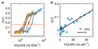
Figure S2: (a) LZ sweep results for various values of $B_{\text{ext}}$. The energy ramp rate $\mathrm{d}J/\mathrm{d}t$ is calibrated using the experimentally-measured spin funnel. (b) The gap $\varDelta_{\text{ST}}$ is extracted by fitting the previous data for $P(T)<0.15$ using Eq. (S1). This example is for $B_{\text{ext}}=5\text{ mT}$.

The gap $\varDelta_{\text{ST}}$ can be probed using Landau-Zener-Stückelberg-Majorana (LZ) transitions Shevchenko et al. (2010). The pulse sequence is shown in the main text Fig. 4. It consists of using a varying ramp rate through the $S{-}T_{-}$ transition, followed by a diabatic ramp back into $(2,0)$. The LZ probability of staying in the same state is $P_{\text{LZ}}=\exp\left[-(2\pi\varDelta_{\text{ST}})^{2}/(h\mathrm{d}E/\mathrm{d}t)\right]$, where $\mathrm{d}E/\mathrm{d}t$ is the energy ramp rate evaluated at the $S{-}T_{-}$ anticrossing Zener (1932). We note that $\mathrm{d}E/\mathrm{d}t=\mathrm{d}J/\mathrm{d}t$, with $J$ the exchange interaction measured from the spin funnel. After the pulse, $P(T)=1-P_{\text{LZ}}$. In Fig. S2(b), we show the result of such pulses for various values of $B_{\text{ext}}$. The $P(T)$ saturates close to $0.5$ rather than $1$. This has been attributed to charge noise by Nichol et al. (2015). To mitigate the impact of this on the gap extraction procedure, we fit only the values for which $P(T)<0.15$. The formula above can be simplified to

$$P(T)=\frac{(2\pi\varDelta_{\text{ST}})^{2}}{h\mathrm{d}E/\mathrm{d}t}.$$ (S1)

This formula is used to extract the gap in Fig. S2(b).

We plot the values obtained for $\varDelta_{\text{ST}}$ against the magnetic field in main text Fig. 4(e). We find that the largest source of error is the probability calibration. The confidence interval is obtained by repeating the fit procedure using extremal values for the probability. The result is a moderate error in the scale of $\varDelta_{\text{ST}}$ that is consistent throughout the range, and hence it does not qualitatively affect the result. The resulting data is fit to a simple model that includes a constant spin-orbit term $\varOmega_{\text{SO}}$ and charge hybridization Nichol et al. (2015),

$$\varDelta_{\text{ST}}=\varOmega_{\text{SO}}\sin\Theta\sin\xi,$$ (S2)

where $\Theta=\arctan(B_{\text{ext}}/t_{\text{c}})$ and $\xi$ is the double QD angle with respect to crystallographic axes. We obtain a value of $\varOmega_{\text{SO}}\sin\xi=113\pm 22\text{ neV}$. Due to the absence of a vector magnet, it was not possible to obtain the full angular dependence. The origin of the angle $\xi$ is therefore undetermined Rančić and Burkard (2014). In our analysis, we neglect the effect of residual ²⁹Si spins, because these are expected to contribute less than a nanoelectronvolt to this gap Witzel et al. (2010); Assali et al. (2011). Experimentally, we can bound the hyperfine contribution to less than $5\text{ neV}$ using a formula as in Nichol et al. (2015).

We can use the relation $\lambda_{\text{SO}}=(t_{\text{c}}d)/(\sqrt{2}\varOmega_{\text{SO}})$, where $d$ is half of the interdot spacing, to estimate a spin-orbit length Fasth et al. (2007); Nichol et al. (2015). Using $d\approx 30\text{ nm}$, and neglecting the angular factor for $\varOmega_{\text{SO}}\sin\xi$, we find $\lambda_{\text{SO}}\approx 1\text{ }\upmu\text{m}$.

S4 Relaxation time

The relaxation and excitation time $T_{1}$ of the $S{-}T_{0}$ qubit was measured both for this device and the one of Jock et al. (2018) using SAP preparation and readout (as described in Fig. S1 but varying $t_{\text{manip}}$). We obtain values in the range of 30 to $100\text{ }\upmu\text{s}$ in the regime where exchange is suppressed. These $T_{1}$ values are consistent with measured Hahn spin echo $T_{2}$ that seem limited by $T_{1}$. For the device featured in the main text, $T_{1}$ becomes larger as exchange is turned on, see Fig. S3. This suggests that the relaxation and excitation mechanism limiting $T_{1}$ is suppressed when $J\gg\Delta E_{z}$. These results contrast with measurements by Dial et al. (2013, see supplement) that show $T_{1}$ increasing to milliseconds when $J\ll\Delta E_{z}$. The exact mechanism remains unclear at the moment; however, we note that the relaxation and excitation seems limited to the $\{\left|S\right>,\left|T_{0}\right>\}$ subspace, as opposed to single-spin relaxation leading to a $\left|T_{-}\right>$ ground state. This hints at a fluctuation of the quantization axis $\Delta E_{z}$ itself, hypothetically due to charge noise or other electric fluctuations, which would couple through the microscopic details of the spin-orbit interaction at the interface. This would be consistent with the suppression of this decoherence when the quantization axis is dominated by $J$.

Figure S3: Relaxation time $T_{1}$ as a function of the detuning in the $(1,1)$ charge configuration. The point where $J=\Delta E_{z}$ (dashed line) is inferred from coherent manipulation experiments.

S5 Dynamic nuclear polarization

As a complementary experiment, we have looked for signatures of DDNP. This effect has been used in GaAs devices to prolong the spin coherence time Bluhm et al. (2010) and induce a $\Delta E_{z}$ for qubit control Foletti et al. (2009). It was shown that spin-orbit interaction can quench the ability to perform DDNP in double-QD devices Nichol et al. (2015).

For our silicon enrichment level, we expect that the maximum polarization achievable by flipping all nuclear spins in opposite ways is approximately $1\text{ MHz}$ Assali et al. (2011). This is an impractical extremal scenario. We instead expect that the polarization could reach fractions of this value in a steady-state pump-probe experiment. The pump-probe experiment consists of one or many cycles of pseudo-SAP ramps through the $S{-}T_{-}$ anticrossing to “pump” the nuclear spins, followed by a probe cycle where the frequency of potential $S{-}T_{0}$ rotations is measured by varying the rotation time. The continuous repetitions should result in a steady-state polarization that could (i) enhance the qubit coherence time by slowing down the $S{-}T_{0}$ mixing, and/or (ii) result in a non-vanishing average $S{-}T_{0}$ rotation frequency.

Here we list some of the parameters used in our trials. We used two fields of $0.4\text{ mT}$ and $150\text{ mT}$. We interleaved one, two and three pump cycles with the probe cycle, and compared the results with those without pump cycles. The data was averaged in each case for periods of up to 6 hours of continuous pump-probing. A few ramp rates were tried, including one that aims at a moderate $P(T)\approx 0.3$ to avoid long incoherent mixing (pseudo-SAP).

In none of the results did we find meaningful differences between the pump and no-pump cases. This is not surprising, in light of the work of Nichol et al. (2015), and suggests a spin-orbit origin of the $S{-}T_{-}$ mixing and quenching of DDNP by spin-orbit interaction.

S6 Spin-orbit interaction model

Consider sitting at an interdot detuning $\epsilon$ that is well within the $(1,1)$ charge configuration, wherein $\epsilon$ is much larger than the interdot tunnel coupling $t$, $\epsilon\gg t$. In this case, we can approximate the two-electron states as being composed of the single-particle eigenstates of either the left (L) or right (R) quantum dots. Suppose, for now, that the valley splitting in the left dot, $\Delta_{\mathrm{vs},L}$ is significantly larger than for the right dot, $\Delta_{\mathrm{vs},R}$. As a consequence, the relevant low-energy excited state we ought to include is the excited valley state of the second dot, $|{\phi_{R^{*}}}\rangle$. In the following, we take the convention that the spin configuration $|{\uparrow}\rangle$ is oriented along the $\hat{z}$ crystallographic axis normal to the two-dimensional electron gas plane. The relevant $(1,1)$ two-electron states involving the ground valley states, $|{\phi_{L}}\rangle$, $|{\phi_{R}}\rangle$ are the following:

$$|{S(1,1)}\rangle = \frac{1}{2}\big{(}|{\phi_{L}\phi_{R}}\rangle+|{\phi_{R}\phi_{L}}\rangle\big{)}\big{(}|{\uparrow\downarrow}\rangle-|{\downarrow\uparrow}\rangle\big{)}$$ (S3)

$$|{T_{0}(1,1)}\rangle = \frac{1}{2}\big{(}|{\phi_{L}\phi_{R}}\rangle-|{\phi_{R}\phi_{L}}\rangle\big{)}\big{(}|{\uparrow\downarrow}\rangle+|{\downarrow\uparrow}\rangle\big{)}$$ (S4)

$$|{T_{+}(1,1)}\rangle = \frac{1}{\sqrt{2}}\big{(}|{\phi_{L}\phi_{R}}\rangle-|{\phi_{R}\phi_{L}}\rangle\big{)}|{\uparrow\uparrow}\rangle$$ (S5)

$$|{T_{-}(1,1)}\rangle = \frac{1}{\sqrt{2}}\big{(}|{\phi_{L}\phi_{R}}\rangle-|{\phi_{R}\phi_{L}}\rangle\big{)}|{\downarrow\downarrow}\rangle,$$ (S6)

while the relevant (1,1) two-electron states that involve the excited single-particle valley state $|{\phi_{R^{*}}}\rangle$ are

$$|{S^{*}(1,1)}\rangle = \frac{1}{2}\big{(}|{\phi_{L}\phi_{R^{*}}}\rangle+|{\phi_{R^{*}}\phi_{L}}\rangle\big{)}\big{(}|{\uparrow\downarrow}\rangle-|{\downarrow\uparrow}\rangle\big{)}$$ (S7)

$$|{T_{0}^{*}(1,1)}\rangle = \frac{1}{2}\big{(}|{\phi_{L}\phi_{R^{*}}}\rangle-|{\phi_{R^{*}}\phi_{L}}\rangle\big{)}\big{(}|{\uparrow\downarrow}\rangle+|{\downarrow\uparrow}\rangle\big{)}$$ (S8)

$$|{T_{+}^{*}(1,1)}\rangle = \frac{1}{\sqrt{2}}\big{(}|{\phi_{L}\phi_{R^{*}}}\rangle-|{\phi_{R^{*}}\phi_{L}}\rangle\big{)}|{\uparrow\uparrow}\rangle$$ (S9)

$$|{T_{-}^{*}(1,1)}\rangle = \frac{1}{\sqrt{2}}\big{(}|{\phi_{L}\phi_{R^{*}}}\rangle-|{\phi_{R^{*}}\phi_{L}}\rangle\big{)}|{\downarrow\downarrow}\rangle.$$ (S10)

We choose Cartesian coordinates $x,y,z$ defined along the crystallographic directions $[100]$, $[010]$ and $[001]$, respectively, and with $[001]$ perpendicular to the interface. This is shown in Fig. S4. Let the applied magnetic field be given by

$$\mathbf{B}=(B_{x},B_{y},B_{z})=B\big{(}\sin(\theta)\cos(\varphi),\sin(\theta)\sin(\varphi),\cos(\theta)\big{)}.$$ (S11)

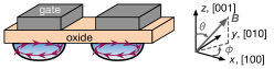
Figure S4: Model coordinates system. The double QD axis is oriented close to the [110] crystallographic axis.

The full $8\times 8$ Hamiltonian describing the $(1,1)$ charge sector is given by the following, in the basis

$$\mathcal{H}_{(1,1)}=\mathrm{span}\{S(1,1),T_{0}(1,1),T_{+}(1,1),T_{-}(1,1),S^{*}(1,1),T_{0}^{*}(1,1),T_{+}^{*}(1,1),T_{-}^{*}(1,1)\},$$ (S12)

and

$$H=\left(\begin{array}[]{cc}H_{\mathrm{GG}}&H_{\mathrm{GE}}\\ H_{\mathrm{GE}}^{\dagger}&H_{\mathrm{EE}}\end{array}\right),$$ (S13)

where

$$H_{\mathrm{GG}}=\left(\begin{array}[]{cccc}0&0&-\frac{1}{\sqrt{2}}(h_{\downarrow\uparrow}^{LL}-h_{\downarrow\uparrow}^{RR})&\frac{1}{\sqrt{2}}(h_{\uparrow\downarrow}^{LL}-h_{\uparrow\downarrow}^{RR})\\ \cdot&J_{11}&\frac{1}{\sqrt{2}}(h_{\downarrow\uparrow}^{LL}+h_{\downarrow\uparrow}^{RR})+\frac{1}{\sqrt{2}}g\mu_{B}(B_{x}+iB_{y})&\frac{1}{\sqrt{2}}(h_{\uparrow\downarrow}^{LL}+h_{\uparrow\downarrow}^{RR})+\frac{1}{\sqrt{2}}g\mu_{B}(B_{x}-iB_{y})\\ \cdot&\cdot&J_{11}+g\mu_{B}B_{z}&0\\ \cdot&\cdot&\cdot&J_{11}-g\mu_{B}B_{z}\end{array}\right),$$ (S14)

$$H_{\mathrm{GE}}=\left(\begin{array}[]{cccc}0&0&\frac{1}{\sqrt{2}}h_{\downarrow\uparrow}^{RR^{*}}&-\frac{1}{\sqrt{2}}h_{\uparrow\downarrow}^{RR^{*}}\\ 0&0&\frac{1}{\sqrt{2}}h_{\downarrow\uparrow}^{RR^{*}}&\frac{1}{\sqrt{2}}h_{\uparrow\downarrow}^{RR^{*}}\\ \frac{1}{\sqrt{2}}h_{\uparrow\downarrow}^{RR^{*}}&-\frac{1}{\sqrt{2}}h_{\uparrow\downarrow}^{RR^{*}}&0&0\\ -\frac{1}{\sqrt{2}}h_{\downarrow\uparrow}^{RR^{*}}&\frac{1}{\sqrt{2}}h_{\downarrow\uparrow}^{RR^{*}}&0&0\end{array}\right),$$ (S15)

$$H_{\mathrm{EE}}=\left(\begin{array}[]{cccc}\Delta_{\mathrm{vs},R}&0&-\frac{1}{\sqrt{2}}(h_{\downarrow\uparrow}^{LL}-h_{\downarrow\uparrow}^{R^{*}R^{*}})&\frac{1}{\sqrt{2}}(h_{\uparrow\downarrow}^{LL}-h_{\uparrow\downarrow}^{R^{*}R^{*}})\\ \cdot&\Delta_{\mathrm{vs},R}+J_{11}&\frac{1}{\sqrt{2}}(h_{\downarrow\uparrow}^{LL}+h_{\downarrow\uparrow}^{R^{*}R^{*}})+\frac{1}{\sqrt{2}}g\mu_{B}(B_{x}+iB_{y})&\frac{1}{\sqrt{2}}(h_{\uparrow\downarrow}^{LL}+h_{\uparrow\downarrow}^{R^{*}R^{*}})+\frac{1}{\sqrt{2}}g\mu_{B}(B_{x}-iB_{y})\\ \cdot&\cdot&\Delta_{\mathrm{vs},R}+J_{11}+g\mu_{B}B_{z}&0\\ \cdot&\cdot&\cdot&\Delta_{\mathrm{vs},R}+J_{11}-g\mu_{B}B_{z}\end{array}\right).$$ (S16)

Here $J_{11}$ parameterizes the residual exchange energy at the given operating point in the $(1,1)$ configuration, $\mu_{B}=57.88\ \mathrm{\mu eV\,T}^{-1}$ is the Bohr magneton, $g=2$ is the $g$-factor of bulk Si, and

$$h_{s_{1}s_{2}}^{MN}=\langle\phi_{M}s_{1}|H_{\mathrm{SO}}|\phi_{N}s_{2}\rangle$$ (S17)

with $s_{1},s_{2}\in\{\uparrow,\downarrow\}$, $M,N\in\{L,R,R^{*}\}$. The spin-orbit coupling Hamiltonian $H_{\mathrm{SO}}$ is given by

$$H_{\mathrm{SO}} = H_{R}+H_{D}$$ (S18)

$$= \delta(z)\big{[}\gamma_{R}(P_{y}\sigma_{x}-P_{x}\sigma_{y})+\gamma_{D}(P_{x}\sigma_{x}-P_{y}\sigma_{y})\big{]},$$ (S19)

with $z=0$ denoting the position of the Si/SiO₂ interface and $P_{x},P_{y}$ the kinetic momenta along the $\hat{x}$ and $\hat{y}$ crystallographic axes.

We now turn our attention to evaluating the matrix elements Eq. (S17). Since $|{\phi_{R}}\rangle$ and $|{\phi_{R^{*}}}\rangle$ are the ground and first excited valley states of the right dot, respectively, and occupy the two-dimensional $\pm z$ valley subspace, we can express them as

$$\langle\mathbf{r}|\phi_{R}\rangle = \frac{1}{\sqrt{2}}\big{(}e^{ik_{0}z}+e^{i\varphi_{v,\mathrm{R}}}e^{-ik_{0}z}\big{)}\psi_{R}(\mathbf{r})$$ (S20)

$$\langle\mathbf{r}|\phi_{R^{*}}\rangle = \frac{1}{\sqrt{2}}\big{(}e^{ik_{0}z}-e^{i\varphi_{v,\mathrm{R}}}e^{-ik_{0}z}\big{)}\psi_{R}(\mathbf{r}),$$ (S21)

where $\varphi_{v,\mathrm{R}}$ denotes a valley phase factor (relative complex phase between the $+z$ and $-z$ valley components) for the right dot and $\psi_{R}(\mathbf{r})$ is an envelope function that is common to these two lowest valley eigenstates. Similarly, for the left dot we have

$$\langle\mathbf{r}|\phi_{L}\rangle=\frac{1}{\sqrt{2}}\big{(}e^{ik_{0}z}+e^{i\varphi_{v,\mathrm{L}}}e^{-ik_{0}z}\big{)}\psi_{L}(\mathbf{r}).$$ (S22)

Evaluating the interface-localized momentum matrix elements for these valley eigenstates along the lines of the analysis in Jock et al. (2018), we have

$$\langle\phi_{L}|\delta(z)P_{k}|\phi_{L}\rangle = (1+\cos(\varphi_{v,\mathrm{L}}))\langle\psi_{L}|\delta(z)P_{k}|\psi_{L}\rangle$$ (S23)

$$\langle\phi_{R}|\delta(z)P_{k}|\phi_{R}\rangle = (1+\cos(\varphi_{v,\mathrm{R}}))\langle\psi_{R}|\delta(z)P_{k}|\psi_{R}\rangle$$ (S24)

$$\langle\phi_{R}|\delta(z)P_{k}|\phi_{R^{*}}\rangle = -i\sin(\varphi_{v,\mathrm{R}})\langle\psi_{R}|\delta(z)P_{k}|\psi_{R}\rangle,$$ (S25)

with $k\in\{x,y\}$ and where $\langle\psi_{R}|\delta(z)P_{x,y}|\psi_{R}\rangle$ are matrix elements that are proportional to the applied magnetic field. These latter factors also depend on lateral confinement and vertical electric field, wrapped into the parameters $\lambda^{x,y}$:

$$\langle\psi_{L}|\delta(z)P_{x}|\psi_{L}\rangle = \lambda_{L}^{x}B_{y}$$ (S26)

$$\langle\psi_{L}|\delta(z)P_{y}|\psi_{L}\rangle = -\lambda_{L}^{y}B_{x}$$ (S27)

$$\langle\psi_{R}|\delta(z)P_{x}|\psi_{R}\rangle = \lambda_{R}^{x}B_{y}$$ (S28)

$$\langle\psi_{R}|\delta(z)P_{y}|\psi_{R}\rangle = -\lambda_{R}^{y}B_{x}.$$ (S29)

In the following, we will assume that the left and right dots are nearly symmetric, such that $\lambda_{L}^{x}=\lambda_{L}^{y}=\lambda_{L}$ and $\lambda_{R}^{x}=\lambda_{R}^{y}=\lambda_{R}$. Defining the Rashba and Dresselhaus spin-orbit (SO) coupling strengths for the left and right dots as

$$\alpha^{L}=\gamma_{R}\lambda_{L}$$ (S30)

$$\alpha^{R}=\gamma_{R}\lambda_{R}$$ (S31)

$$\beta^{L}=\gamma_{D}\lambda_{L}$$ (S32)

$$\beta^{R}=\gamma_{D}\lambda_{R},$$ (S33)

we have

$$h_{\downarrow\uparrow}^{LL} = (1+\cos(\varphi_{v,\mathrm{L}}))\big{[}-\alpha^{L}(B_{x}+iB_{y})+\beta^{L}(B_{y}+iB_{x})\big{]}$$ (S34)

$$h_{\uparrow\downarrow}^{LL} = (1+\cos(\varphi_{v,\mathrm{L}}))\big{[}-\alpha^{L}(B_{x}-iB_{y})+\beta^{L}(B_{y}-iB_{x})\big{]}$$ (S35)

$$h_{\downarrow\uparrow}^{RR} = (1+\cos(\varphi_{v,\mathrm{R}}))\big{[}-\alpha^{R}(B_{x}+iB_{y})+\beta^{R}(B_{y}+iB_{x})\big{]}$$ (S36)

$$h_{\uparrow\downarrow}^{RR} = (1+\cos(\varphi_{v,\mathrm{R}}))\big{[}-\alpha^{R}(B_{x}-iB_{y})+\beta^{R}(B_{y}-iB_{x})\big{]}$$ (S37)

$$h_{\downarrow\uparrow}^{RR^{*}} = -i\sin(\varphi_{v,\mathrm{R}})\big{[}-\alpha^{R}(B_{x}+iB_{y})+\beta^{R}(B_{y}+iB_{x})\big{]}$$ (S38)

$$h_{\uparrow\downarrow}^{RR^{*}} = -i\sin(\varphi_{v,\mathrm{R}})\big{[}-\alpha^{R}(B_{x}-iB_{y})+\beta^{R}(B_{y}-iB_{x})\big{]}$$ (S39)

$$h_{\downarrow\uparrow}^{R^{*}R^{*}} = (1-\cos(\varphi_{v,\mathrm{R}}))\big{[}-\alpha^{R}(B_{x}+iB_{y})+\beta^{R}(B_{y}+iB_{x})\big{]}$$ (S40)

$$h_{\uparrow\downarrow}^{R^{*}R^{*}} = (1-\cos(\varphi_{v,\mathrm{R}}))\big{[}-\alpha^{R}(B_{x}-iB_{y})+\beta^{R}(B_{y}-iB_{x})\big{]}.$$ (S41)

We now have explicit expressions for all matrix elements of the Hamiltonian Eq. (S13). Note that we have shown that the intravalley and intervalley spin-orbit coupling (SOC) matrix elements all scale linearly with the applied magnetic field, following an extended version of the analysis previously detailed in Jock et al. (2018).

S6.1 Reduced-dimensional model

Since we are interested primarily in the two-dimensional space spanned by the lowest-energy singlet and unpolarized triplet states, to arrive at an analytic expression for the ST rotation frequency we now evaluate perturbatively the action of these other six states on our qubit subspace through intravalley and intervalley spin-orbit coupling. First, we transform our basis from the original spin basis defined with respect to the $z$-axis, given in Eq. (S12), into the spin basis defined by the applied magnetic field, $\mathbf{B}=B(\sin(\theta)\cos(\varphi),\sin(\theta)\sin(\varphi),\cos(\theta))$. In the following, we use a tilde to denote states associated with the spin basis determined by the applied magnetic field or operators defined in this basis. Diagonalizing the $2\times 2$ Zeeman Hamiltonian to obtain the spin eigenstates associated with the applied magnetic field orientation,

$$H_{\mathrm{Zee}}=\left(\begin{array}[]{cc}\cos{\theta}&e^{-i\varphi}\sin{\theta}\\ e^{i\varphi}\sin{\theta}&-\cos{\theta}\end{array}\right),$$ (S42)

we have

$$|{\tilde{\uparrow}}\rangle = e^{-i\varphi/2}\cos{(\theta/2)}|{\uparrow}\rangle+e^{i\varphi/2}\sin{(\theta/2)}|{\downarrow}\rangle$$ (S43)

$$|{\tilde{\downarrow}}\rangle = -e^{-i\varphi/2}\sin{(\theta/2)}|{\uparrow}\rangle+e^{i\varphi/2}\cos{(\theta/2)}|{\downarrow}\rangle$$ (S44)

and hence

$$|{\tilde{T}_{-}(1,1)}\rangle = e^{-i\varphi}\sin^{2}\left(\frac{\theta}{2}\right)|{T_{+}(1,1)}\rangle+e^{i\varphi}\cos^{2}\left(\frac{\theta}{2}\right)|{T_{-}(1,1)}\rangle-\frac{1}{\sqrt{2}}\sin{\theta}|{T_{0}(1,1)}\rangle$$

$$|{\tilde{S}(1,1)}\rangle = |{S(1,1)}\rangle$$

$$|{\tilde{T}_{0}(1,1)}\rangle = \cos{\theta}|{T_{0}(1,1)}\rangle+\frac{1}{\sqrt{2}}\sin{\theta}\big{(}e^{i\varphi}|{T_{-}(1,1)}\rangle-e^{-i\varphi}|{T_{+}(1,1)}\rangle\big{)}$$

$$|{\tilde{T}_{+}(1,1)}\rangle = e^{-i\varphi}\cos^{2}\left(\frac{\theta}{2}\right)|{T_{+}(1,1)}\rangle+e^{i\varphi}\sin^{2}\left(\frac{\theta}{2}\right)|{T_{-}(1,1)}\rangle+\frac{1}{\sqrt{2}}\sin{\theta}|{T_{0}(1,1)}\rangle$$

$$|{\tilde{T}_{-}^{*}(1,1)}\rangle = e^{-i\varphi}\sin^{2}\left(\frac{\theta}{2}\right)|{T_{+}^{*}(1,1)}\rangle+e^{i\varphi}\cos^{2}\left(\frac{\theta}{2}\right)|{T_{-}^{*}(1,1)}\rangle-\frac{1}{\sqrt{2}}\sin{\theta}|{T_{0}^{*}(1,1)}\rangle$$

$$|{\tilde{S}^{*}(1,1)}\rangle = |{S^{*}(1,1)}\rangle$$

$$|{\tilde{T}_{0}^{*}(1,1)}\rangle = \cos{\theta}|{T_{0}^{*}(1,1)}\rangle+\frac{1}{\sqrt{2}}\sin{\theta}\big{(}e^{i\varphi}|{T_{-}^{*}(1,1)}\rangle-e^{-i\varphi}|{T_{+}^{*}(1,1)}\rangle\big{)}$$

$$|{\tilde{T}_{+}^{*}(1,1)}\rangle = e^{-i\varphi}\cos^{2}\left(\frac{\theta}{2}\right)|{T_{+}^{*}(1,1)}\rangle+e^{i\varphi}\sin^{2}\left(\frac{\theta}{2}\right)|{T_{-}^{*}(1,1)}\rangle+\frac{1}{\sqrt{2}}\sin{\theta}|{T_{0}^{*}(1,1)}\rangle.$$ (S45)

Equivalently, the unitary transformation from the basis $\{S(1,1),T_{0}(1,1),T_{+}(1,1),T_{-}(1,1)\}$ to $\{S(1,1),\tilde{T}_{0}(1,1),\tilde{T}_{+}(1,1),\tilde{T}_{-}(1,1)\}$ is given by the unitary

$$U=\left(\begin{array}[]{cccc}1&0&0&0\\ 0&\cos(\theta)&-\frac{1}{\sqrt{2}}\sin(\theta)e^{i\varphi}&\frac{1}{\sqrt{2}}\sin(\theta)e^{-i\varphi}\\ 0&\frac{1}{\sqrt{2}}\sin(\theta)&\cos^{2}(\theta/2)e^{i\varphi}&\sin^{2}(\theta/2)e^{-i\varphi}\\ 0&-\frac{1}{\sqrt{2}}\sin(\theta)&\sin^{2}(\theta/2)e^{i\varphi}&\cos^{2}(\theta/2)e^{-i\varphi}\end{array}\right).$$ (S46)

Transforming the Hamiltonian Eq. (S13) into the spin basis defined by the applied magnetic field, we have

$$\tilde{H}=\big{(}U\oplus U\big{)}H\big{(}U^{\dagger}\oplus U^{\dagger}\big{)}.$$ (S47)

We can decompose the Hamiltonian into the form $\tilde{H}=\tilde{H}_{0}+\tilde{V}$, where $\tilde{H}_{0}$ includes the bare Zeeman terms, residual exchange splitting $J_{11}$, valley splitting, and direct SOC coupling between the singlet $S$ and unpolarized triplet state $\tilde{T}_{0}$. The term $\tilde{V}$ encodes all other contributions from SOC. The Hamiltonian $\tilde{H}_{0}$ has block form, where $h_{a}$ is a $2\times 2$ matrix operating on the subspace $\mathcal{H}_{a}$ spanned by $\{S,\tilde{T}_{0}\}$ and $h_{b}$ is a diagonal $6\times 6$ matrix operating on the subspace $\mathcal{H}_{b}$ spanned by all other states $\{\tilde{T}_{-},\tilde{T}_{+},S^{*},\tilde{T}_{0}^{*},\tilde{T}_{+}^{*},\tilde{T}_{-}^{*}\}$,

$$\tilde{H}_{0}=\left(\begin{array}[]{cc}h_{a}&0\\ 0&h_{b}\end{array}\right),$$ (S48)

where

$$h_{a}=\left(\begin{array}[]{cc}0&B\sin^{2}(\theta)\big{(}\tilde{\alpha}_{R}-\tilde{\alpha}_{L}-(\tilde{\beta}_{R}-\tilde{\beta}_{L})\sin(2\varphi)\big{)}\\ \cdot&J_{11}\end{array}\right)$$ (S51)

and

$$h_{b}=\mathrm{diag}\left[J_{11}+g\mu_{B}B,J_{11}-g\mu_{B}B,\Delta_{\mathrm{vs},R},\Delta_{\mathrm{vs},R}+J_{11},\Delta_{\mathrm{vs},R}+J_{11}+g\mu_{B}B,\Delta_{\mathrm{vs},R}+J_{11}-g\mu_{B}B\right],$$ (S52)

where we’re using the shorthand notation

$$\tilde{\alpha}^{L} \equiv (1+\cos(\varphi_{v,\mathrm{L}}))\alpha^{L}$$

$$\tilde{\alpha}^{R} \equiv (1+\cos(\varphi_{v,\mathrm{R}}))\alpha^{R}$$

$$\tilde{\beta}^{L} \equiv (1+\cos(\varphi_{v,\mathrm{L}}))\beta^{L}$$

$$\tilde{\beta}^{R} \equiv (1+\cos(\varphi_{v,\mathrm{R}}))\beta^{R}.$$ (S53)

Similarly, the perturbation $\tilde{V}$ is given in block form by

$$\tilde{V}=\left(\begin{array}[]{cc}0&v_{ab}\\ v^{\dagger}_{ab}&v_{b}\end{array}\right),$$ (S54)

where $v_{ab}$ is a $2\times 6$ matrix encoding the SOC between the subspaces $\mathcal{H}_{a}$ and $\mathcal{H}_{b}$ and $v_{b}$ is a $6\times 6$ matrix describing the SOC within the subspace $\mathcal{H}_{b}$. To describe the effect of $\tilde{V}$ on the spectrum of the two-level subspace of interest, we perform a Schrieffer-Wolff transformation. This entails finding an anti-Hermitian operator $S$ such that the unitary transformation $H^{\prime}=e^{S}\tilde{H}e^{-S}$ eliminates the effective coupling between our two-dimensional subspace of interest and all other states. Expanding this transformation in $S$, we have $H^{\prime}=\tilde{H}_{0}+\tilde{V}+[S,\tilde{H}_{0}]+[S,\tilde{V}]+\frac{1}{2}[S,[S,\tilde{H}_{0}]]+\frac{1}{2}[S,[S,\tilde{V}]]$. Hence, to eliminate the off-diagonal block component $v_{ab}$ to lowest order in $S$, we require $[S,\tilde{H}_{0}]=-\tilde{V}$. First, we make the ansatz that $S$ only has nonzero components on the off-diagonal block so that

$$S=\left(\begin{array}[]{cc}0&s_{ab}\\ s_{ba}&0\end{array}\right),$$ (S55)

where $s_{ab}$ is a $2\times 6$ matrix and $s_{ba}=-s_{ab}^{\dagger}$ due to $S$ being anti-Hermitian. Making use of the block structure of these Hamiltonian terms, we obtain the condition $h_{a}s_{ab}-s_{ab}h_{b}=v_{ab}$. Noting that $h_{b}$ is invertible for the range of parameters of interest here, we can rewrite this as a recurrence relation to obtain the form

$$s_{ab}=-\Big{(}\sum_{n=0}^{\infty}h_{a}^{n}v_{ab}h_{b}^{-n}\Big{)}h_{b}^{-1}.$$ (S56)

Retaining only the leading order in $h_{b}^{-1}$, we obtain $s_{ab}\approx-v_{ab}h_{b}^{-1}$. Using this to evaluate the desired $2\times 2$ block of $H^{\prime}$, we obtain

$$h_{a}^{\prime} = h_{a}+\frac{1}{2}s_{ab}v_{ab}^{\dagger}+\frac{1}{2}vs_{ab}^{\dagger}$$

$$\approx h_{a}-v_{ab}h_{b}^{-1}v_{ab}^{\dagger}.$$

In our case, we have

$$v_{ab}^{\dagger}=\frac{B\sin(\theta)}{\sqrt{2}}\left(\begin{array}[]{cc}-\Delta\tilde{\alpha}\cos\theta-\big{(}\sin(2\varphi)\cos\theta+i\cos(2\varphi)\big{)}\Delta\tilde{\beta}&-\sigma\tilde{\alpha}\cos\theta+\big{(}\sin(2\varphi)\cos\theta-i\cos(2\varphi)\big{)}\sigma\tilde{\beta}\\ \Delta\tilde{\alpha}\cos\theta-\big{(}\sin(2\varphi)\cos\theta+i\cos(2\varphi)\big{)}\Delta\tilde{\beta}&-\sigma\tilde{\alpha}\cos\theta+\big{(}\sin(2\varphi)\cos\theta+i\cos(2\varphi)\big{)}\sigma\tilde{\beta}\\ 0&i\sqrt{2}\sin\theta\big{(}\alpha_{R}-\beta_{R}\sin(2\varphi)\big{)}\sin(\varphi_{v,\mathrm{R}})\\ i\sqrt{2}\sin\theta\big{(}\overline{\alpha}_{R}\!-\!\overline{\beta}_{R}\sin(2\varphi)\big{)}&-\sqrt{2}\sin\theta\cos\theta\Big{(}i\overline{\alpha}_{R}+e^{-2i\varphi}\overline{\beta}_{R}\Big{)}\\ \overline{\beta}_{R}\cos(2\varphi)\!-\!i\cos\theta\big{(}\overline{\alpha}_{R}-\overline{\beta}_{R}\sin(2\varphi)\big{)}&\Big{[}\frac{e^{2i\varphi}+e^{-2i\varphi}\cos(2\theta)}{2}\!+\!i\!\sin(2\varphi)\!\cos\theta\Big{]}\overline{\beta}_{R}\!-\!i\overline{\alpha}_{R}\big{(}\!\sin^{2}\theta\!-\!\cos\theta\big{)}\\ \overline{\beta}_{R}\cos(2\varphi)\!+\!i\cos\theta\big{(}\overline{\alpha}_{R}-\overline{\beta}_{R}\sin(2\varphi)\big{)}&\Big{[}\!-\!\frac{e^{2i\varphi}+e^{-2i\varphi}\cos(2\theta)}{2}\!+\!i\!\sin(2\varphi)\!\cos\theta\Big{]}\overline{\beta}_{R}\!+\!i\overline{\alpha}_{R}\big{(}\!\sin^{2}\theta\!-\!\cos\theta\big{)}\par\end{array}\right),$$

where $\Delta\tilde{\alpha}\equiv\tilde{\alpha}_{R}-\tilde{\alpha}_{L}$, $\Delta\tilde{\beta}\equiv\tilde{\beta}_{R}-\tilde{\beta}_{L}$ and $\overline{\beta}_{R}\equiv\beta_{R}\sin(\varphi_{v,\mathrm{R}})$, $\overline{\alpha}_{R}\equiv\alpha_{R}\sin(\varphi_{v,\mathrm{R}})$. Notice that $v_{ab}^{\dagger}$ vanishes completely when the magnetic field is applied normal to the interface ($\theta=0$). Suppose the magnetic field is applied in-plane ($\theta=\pi/2$). For this family of cases, we have

$$v_{ab}^{\dagger}=\frac{B}{\sqrt{2}}\left(\begin{array}[]{cc}-i\cos(2\varphi)\Delta\tilde{\beta}&-i\cos(2\varphi)\sigma\tilde{\beta}\\ -i\cos(2\varphi)\Delta\tilde{\beta}&i\cos(2\varphi)\sigma\tilde{\beta}\\ 0&i\sqrt{2}\big{(}\overline{\alpha}_{R}-\overline{\beta_{R}}\sin(2\varphi)\big{)}\\ i\sqrt{2}\big{(}\overline{\alpha}_{R}-\overline{\beta_{R}}\sin(2\varphi)\big{)}&0\\ \overline{\beta}_{R}\cos(2\varphi)&-i\overline{\alpha}_{R}\\ \overline{\beta}_{R}\cos(2\varphi)&i\overline{\alpha}_{R}\end{array}\right).$$ (S57)

We now consider the two magnetic field orientations considered in this work, $\mathbf{B}\parallel[100]$ and $\mathbf{B}\parallel[110]$. For the case $\mathbf{B}\parallel[100]$ ($\theta=\pi/2$, $\varphi=0$) we have

$$v_{ab}^{\dagger}=\frac{B}{\sqrt{2}}\left(\begin{array}[]{cc}-i\Delta\tilde{\beta}&-i\sigma\tilde{\beta}\\ -i\Delta\tilde{\beta}&i\sigma\tilde{\beta}\\ 0&i\sqrt{2}\overline{\alpha}_{R}\\ i\sqrt{2}\overline{\alpha}_{R}&0\\ \overline{\beta}_{R}&-i\overline{\alpha}_{R}\\ \overline{\beta}_{R}&i\overline{\alpha}_{R}\end{array}\right).$$ (S58)

Similarly, for the case $\mathbf{B}\parallel[110]$ ($\theta=\pi/2$, $\varphi=\pi/4$) we have

$$v_{ab}^{\dagger}=\frac{B}{\sqrt{2}}\left(\begin{array}[]{cc}0&0\\ 0&0\\ 0&i\sqrt{2}\big{(}\overline{\alpha}_{R}-\overline{\beta}_{R}\big{)}\\ i\sqrt{2}\big{(}\overline{\alpha}_{R}-\overline{\beta}_{R}\big{)}&0\\ 0&-i\overline{\alpha}_{R}\\ 0&i\overline{\alpha}_{R}\end{array}\right).$$ (S59)

We can now evaluate the ST rotation frequencies induced by SOC for these two cases. For $\mathbf{B}\parallel[110]$ we have

$$h_{a}^{\prime} = \left(\begin{array}[]{cc}0&B(\Delta\tilde{\alpha}-\Delta\tilde{\beta})\\ B(\Delta\tilde{\alpha}-\Delta\tilde{\beta})&J_{11}-\frac{B^{2}\overline{\alpha}_{R}^{2}\Delta_{\mathrm{vs},R}}{\Delta_{\mathrm{vs},R}^{2}-(g\mu_{B}B)^{2}}\end{array}\right)$$ (S62)

$$\approx \left(\begin{array}[]{cc}0&B(\Delta\tilde{\alpha}-\Delta\tilde{\beta})\\ B(\Delta\tilde{\alpha}-\Delta\tilde{\beta})&J_{11}\end{array}\right),$$ (S65)

if $(B\overline{\alpha}_{R})^{2}/\Delta_{\mathrm{vs},R}\ll 1$. Hence,

$$\Delta_{[110]}\approx\sqrt{4B^{2}(\Delta\tilde{\alpha}-\Delta\tilde{\beta})^{2}+J_{11}^{2}}.$$ (S66)

Similarly, for $\mathbf{B}\parallel[100]$ and assuming contributions only from Dresselhaus SOC, we find

$$\Delta_{[100]}\approx\sqrt{\Bigg{(}\frac{B^{2}\overline{\beta}_{R}^{2}\Delta_{\mathrm{vs},R}}{\Delta_{\mathrm{vs},R}^{2}-(g\mu_{B}B)^{2}}\Bigg{)}^{2}+\Bigg{(}\frac{2B\big{(}\tilde{\beta}_{R}^{2}-\tilde{\beta}_{L}^{2}\big{)}}{g\mu_{B}}\Bigg{)}^{2}}.$$ (S67)

From these expressions, we can see the origin of the generally linear dependence of the rotation frequency on magnetic field magnitude for the [110] orientation and quadratic-like dependence for the [100] orientation. While the number of free model parameters here is too large to be fully constrained by available experimental data, we can obtain a reasonably good fit to the data by assuming vanishingly small Rashba SOC ($|\alpha_{L}|,|\alpha_{R}|\ll|\beta_{L}|,|\beta_{R}|$). This is consistent with Jock et al. (2018). To illustrate the underconstrained nature of the fit, in Fig. S5, we show how equivalently satisfactory fits may be obtained by allowing the valley phases $\varphi_{v,\mathrm{R}},\varphi_{v,\mathrm{L}}$ to differ while holding the underlying Dresselhaus couplings $\beta_{R},\beta_{L}$ to be equal or, alternatively, the converse. We note that the above Eq. (S67) reduces to the main text Eq. (3) for $\Delta_{\mathrm{vs},R}\approx g\mu_{B}B$ and similar Dresselhaus strengths $|\tilde{\beta}_{L}|\approx|\tilde{\beta}_{R}|$. We emphasize that while the model doesn’t uniquely identify some microscopic parameters like the valley phases, the conclusion is that both intravalley and intervalley processes are necessary to explain the data of Fig. 3.

Figure S5: Misfit ($l^{2}$ norm of difference) between model and measured values for the $S{-}T_{0}$ rotation magnetic field dependence. Here, we are setting $\beta_{R}=0.7\ \mathrm{\mu eV/T}$, $\varphi_{v,\mathrm{R}}=\pi/2$, and $\alpha_{L}=\alpha_{R}=0$. The points labeled by $\times$ ($\star$) indicate parameter choices where the misfit is the same but the valley phases (Dresselhaus couplings) are allowed to differ while the Dresselhaus couplings (valley phases) are set to be the same, respectively. For visual clarity, misfits larger than the maximum plotted have been clipped.

S6.2 Model parameters known directly from experiment

The Tab. S2 lists the parameters used to fit the experimental data.

	$\mathbf{B}\parallel[100]$	$\mathbf{B}\parallel[110]$
Triplet-singlet splitting in $(2,0)$, $J_{20}$ ($\mathrm{\mu eV}$)	243	255
Right dot valley splitting, $\Delta_{\mathrm{vs},R}$ ($\mathrm{\mu eV}$)	185	Not characterized
BC interdot lever arm ($\mathrm{\mu eV/mV}$)	90	90
BC voltage at zero detuning ($\mathrm{V}$)	2.9321	2.9533
Singlet tunnel coupling, $t_{S}$ ($\mathrm{\mu eV}$)	10	23
Triplet tunnel coupling, $t_{T}$ ($\mathrm{\mu eV}$)	10	25

Table S2: Known model parameters, estimated from spin funnel and magnetospectroscopy measurements. The valley splitting in the right dot was not independently determined for the [110] magnetic field orientation, but has been assumed in our parameter fitting to be similar to the [100] case. Tunnel couplings here are full gap.

References

- Loss and DiVincenzo (1998) D. Loss and D. P. DiVincenzo, “Quantum computation with quantum dots,” Phys. Rev. A 57, 120 (1998).
- Witzel et al. (2010) W. M. Witzel, M. S. Carroll, A. Morello, L. Cywiński, and S. Das Sarma, “Electron spin decoherence in isotope-enriched silicon,” Phys. Rev. Lett. 105, 187602 (2010).
- Veldhorst et al. (2014) M. Veldhorst, J. C. C. Hwang, C. H. Yang, A. W. Leenstra, B. de Ronde, J. P. Dehollain, J. T. Muhonen, F. E. Hudson, K. M. Itoh, A. Morello, and A. S. Dzurak, “An addressable quantum dot qubit with fault-tolerant control-fidelity,” Nat Nano 9, 981 (2014).
- Zwanenburg et al. (2013) F. A. Zwanenburg, A. S. Dzurak, A. Morello, M. Y. Simmons, L. C. L. Hollenberg, G. Klimeck, S. Rogge, S. N. Coppersmith, and M. A. Eriksson, “Silicon quantum electronics,” Rev. Mod. Phys. 85, 961 (2013).
- Watson et al. (2017) T. F. Watson, B. Weber, Y.-L. Hsueh, L. L. C. Hollenberg, R. Rahman, and M. Y. Simmons, “Atomically engineered electron spin lifetimes of 30 s in silicon,” Science Advances 3, e1602811 (2017).
- Yang et al. (2013) C. H. Yang, A. Rossi, R. Ruskov, N. S. Lai, F. A. Mohiyaddin, S. Lee, C. Tahan, G. Klimeck, A. Morello, and A. S. Dzurak, “Spin-valley lifetimes in a silicon quantum dot with tunable valley splitting,” Nature Communications 4, 2069 (2013).
- Veldhorst et al. (2015) M. Veldhorst, R. Ruskov, C. H. Yang, J. C. C. Hwang, F. E. Hudson, M. E. Flatté, C. Tahan, K. M. Itoh, A. Morello, and A. S. Dzurak, “Spin-orbit coupling and operation of multivalley spin qubits,” Phys. Rev. B 92, 201401 (2015).
- Eng et al. (2015) K. Eng, T. D. Ladd, A. Smith, M. G. Borselli, A. A. Kiselev, B. H. Fong, K. S. Holabird, T. M. Hazard, B. Huang, P. W. Deelman, I. Milosavljevic, A. E. Schmitz, R. S. Ross, M. F. Gyure, and A. T. Hunter, “Isotopically enhanced triple-quantum-dot qubit,” Science Advances 1, e1500214 (2015).
- Ferdous et al. (2018) R. Ferdous, E. Kawakami, P. Scarlino, M. Nowak, D. R. Ward, D. E. Savage, M. G. Lagally, S. N. Coppersmith, M. Friesen, M. A. Eriksson, L. M. K. Vandersypen, and R. Rahman, “Valley dependent anisotropic spin splitting in silicon quantum dots,” npj Quantum Information 4, 26 (2018).
- Jock et al. (2018) R. M. Jock, N. T. Jacobson, P. Harvey-Collard, A. M. Mounce, V. Srinivasa, D. R. Ward, J. Anderson, R. Manginell, J. R. Wendt, M. Rudolph, T. Pluym, J. K. Gamble, A. D. Baczewski, W. M. Witzel, and M. S. Carroll, “A silicon metal-oxide-semiconductor electron spin-orbit qubit,” Nature Communications 9, 1768 (2018).
- Corna et al. (2018) A. Corna, L. Bourdet, R. Maurand, A. Crippa, D. Kotekar-Patil, H. Bohuslavskyi, R. Laviéville, L. Hutin, S. Barraud, X. Jehl, M. Vinet, S. De Franceschi, Y.-M. Niquet, and M. Sanquer, “Electrically driven electron spin resonance mediated by spin–valley–orbit coupling in a silicon quantum dot,” npj Quantum Information 4, 6 (2018).
- Rössler and Kainz (2002) U. Rössler and J. Kainz, “Microscopic interface asymmetry and spin-splitting of electron subbands in semiconductor quantum structures,” Solid State Communications 121, 313 (2002).
- Prada et al. (2011) M. Prada, G. Klimeck, and R. Joynt, “Spin–orbit splittings in Si/SiGe quantum wells: from ideal Si membranes to realistic heterostructures,” New Journal of Physics 13, 013009 (2011).
- Levy (2002) J. Levy, “Universal quantum computation with spin- pairs and Heisenberg exchange,” Phys. Rev. Lett. 89, 147902 (2002).
- Petta et al. (2005) J. R. Petta, A. C. Johnson, J. M. Taylor, E. A. Laird, A. Yacoby, M. D. Lukin, C. M. Marcus, M. P. Hanson, and A. C. Gossard, “Coherent manipulation of coupled electron spins in semiconductor quantum dots,” Science 309, 2180 (2005).
- Li et al. (2018) R. Li, L. Petit, D. P. Franke, J. P. Dehollain, J. Helsen, M. Steudtner, N. K. Thomas, Z. R. Yoscovits, K. J. Singh, S. Wehner, L. M. K. Vandersypen, J. S. Clarke, and M. Veldhorst, “A crossbar network for silicon quantum dot qubits,” Science Advances 4, eaar3960 (2018).
- Shulman et al. (2012) M. D. Shulman, O. E. Dial, S. P. Harvey, H. Bluhm, V. Umansky, and A. Yacoby, “Demonstration of entanglement of electrostatically coupled singlet-triplet qubits,” Science 336, 202 (2012).
- Srinivasa and Taylor (2015) V. Srinivasa and J. M. Taylor, “Capacitively coupled singlet-triplet qubits in the double charge resonant regime,” Phys. Rev. B 92, 235301 (2015).
- Nichol et al. (2017) J. M. Nichol, L. A. Orona, S. P. Harvey, S. Fallahi, G. C. Gardner, M. J. Manfra, and A. Yacoby, “High-fidelity entangling gate for double-quantum-dot spin qubits,” npj Quantum Information 3, 3 (2017).
- Trifunovic et al. (2012) L. Trifunovic, O. Dial, M. Trif, J. R. Wootton, R. Abebe, A. Yacoby, and D. Loss, “Long-distance spin-spin coupling via floating gates,” Phys. Rev. X 2, 011006 (2012).
- Mehl et al. (2014) S. Mehl, H. Bluhm, and D. P. DiVincenzo, “Two-qubit couplings of singlet-triplet qubits mediated by one quantum state,” Phys. Rev. B 90, 045404 (2014).
- Srinivasa et al. (2015) V. Srinivasa, H. Xu, and J. M. Taylor, “Tunable spin-qubit coupling mediated by a multielectron quantum dot,” Phys. Rev. Lett. 114, 226803 (2015).
- Malinowski et al. (2018) F. K. Malinowski, F. Martins, T. B. Smith, S. D. Bartlett, A. C. Doherty, P. D. Nissen, S. Fallahi, G. C. Gardner, M. J. Manfra, C. M. Marcus, and F. Kuemmeth, “Spin of a multielectron quantum dot and its interaction with a neighboring electron,” Phys. Rev. X 8, 011045 (2018).
- Taylor et al. (2007) J. M. Taylor, J. R. Petta, A. C. Johnson, A. Yacoby, C. M. Marcus, and M. D. Lukin, “Relaxation, dephasing, and quantum control of electron spins in double quantum dots,” Phys. Rev. B 76, 035315 (2007).
- Bluhm et al. (2010) H. Bluhm, S. Foletti, D. Mahalu, V. Umansky, and A. Yacoby, “Enhancing the coherence of a spin qubit by operating it as a feedback loop that controls its nuclear spin bath,” Phys. Rev. Lett. 105, 216803 (2010).
- Shulman et al. (2014) M. D. Shulman, S. P. Harvey, J. M. Nichol, S. D. Bartlett, A. C. Doherty, V. Umansky, and A. Yacoby, “Suppressing qubit dephasing using real-time Hamiltonian estimation,” Nat Commun 5, 5156 (2014).
- Foletti et al. (2009) S. Foletti, H. Bluhm, D. Mahalu, V. Umansky, and A. Yacoby, “Universal quantum control of two-electron spin quantum bits using dynamic nuclear polarization,” Nat Phys 5, 903 (2009).
- Gullans et al. (2010) M. Gullans, J. J. Krich, J. M. Taylor, H. Bluhm, B. I. Halperin, C. M. Marcus, M. Stopa, A. Yacoby, and M. D. Lukin, “Dynamic nuclear polarization in double quantum dots,” Phys. Rev. Lett. 104, 226807 (2010).
- Stepanenko et al. (2012) D. Stepanenko, M. Rudner, B. I. Halperin, and D. Loss, “Singlet-triplet splitting in double quantum dots due to spin-orbit and hyperfine interactions,” Phys. Rev. B 85, 075416 (2012).
- Rančić and Burkard (2014) M. J. Rančić and G. Burkard, “Interplay of spin-orbit and hyperfine interactions in dynamical nuclear polarization in semiconductor quantum dots,” Phys. Rev. B 90, 245305 (2014).
- Nichol et al. (2015) J. M. Nichol, S. P. Harvey, M. D. Shulman, A. Pal, V. Umansky, E. I. Rashba, B. I. Halperin, and A. Yacoby, “Quenching of dynamic nuclear polarization by spin-orbit coupling in GaAs quantum dots,” Nat Commun 6, 7682 (2015).
- Ruskov et al. (2018) R. Ruskov, M. Veldhorst, A. S. Dzurak, and C. Tahan, “Electron -factor of valley states in realistic silicon quantum dots,” Phys. Rev. B 98, 245424 (2018).
- Harvey-Collard et al. (2018) P. Harvey-Collard, B. D’Anjou, M. Rudolph, N. T. Jacobson, J. Dominguez, G. A. Ten Eyck, J. R. Wendt, T. Pluym, M. P. Lilly, W. A. Coish, M. Pioro-Ladrière, and M. S. Carroll, “High-fidelity single-shot readout for a spin qubit via an enhanced latching mechanism,” Phys. Rev. X 8, 021046 (2018).
- Curry et al. (2015) M. J. Curry, T. D. England, N. C. Bishop, G. Ten-Eyck, J. R. Wendt, T. Pluym, M. P. Lilly, S. M. Carr, and M. S. Carroll, “Cryogenic preamplification of a single-electron-transistor using a silicon-germanium heterojunction-bipolar-transistor,” Applied Physics Letters 106, 203505 (2015).
- Assali et al. (2011) L. V. C. Assali, H. M. Petrilli, R. B. Capaz, B. Koiller, X. Hu, and S. Das Sarma, “Hyperfine interactions in silicon quantum dots,” Phys. Rev. B 83, 165301 (2011).
- Rudolph et al. (2016) M. Rudolph, P. Harvey-Collard, R. Jock, T. Jacobson, J. Wendt, T. Pluym, J. Domínguez, G. Ten-Eyck, R. Manginell, M. P. Lilly, and M. S. Carroll, “Coupling MOS quantum dot and phosphorous donor qubit systems,” in 2016 IEEE International Electron Devices Meeting (IEDM) (2016) pp. 34.1.1–34.1.4.
- Harvey-Collard et al. (2017) P. Harvey-Collard, R. M. Jock, N. T. Jacobson, A. D. Baczewski, A. M. Mounce, M. J. Curry, D. R. Ward, J. M. Anderson, R. P. Manginell, J. R. Wendt, M. Rudolph, T. Pluym, M. P. Lilly, M. Pioro-Ladrière, and M. S. Carroll, “All-electrical universal control of a double quantum dot qubit in silicon MOS,” in 2017 IEEE International Electron Devices Meeting (IEDM) (2017) pp. 36.5.1–36.5.4.
- Hao et al. (2014) X. Hao, R. Ruskov, M. Xiao, C. Tahan, and H. Jiang, “Electron spin resonance and spin-valley physics in a silicon double quantum dot,” Nat Commun 5, 3860 (2014).
- Shevchenko et al. (2010) S. Shevchenko, S. Ashhab, and F. Nori, “Landau–Zener–Stückelberg interferometry,” Physics Reports 492, 1 (2010).
- Mehl and DiVincenzo (2014) S. Mehl and D. P. DiVincenzo, “Inverted singlet-triplet qubit coded on a two-electron double quantum dot,” Phys. Rev. B 90, 195424 (2014).
- Note (1) See Supplemental Material for additional details about slow and rapid adiabatic passage, pulse sequence details, measurement of the gap, relaxation time, dynamic nuclear polarization, and spin-orbit interaction model, which includes Refs. Zener (1932); Fasth et al. (2007); Dial et al. (2013).
- Qi et al. (2017) Z. Qi, X. Wu, D. R. Ward, J. R. Prance, D. Kim, J. K. Gamble, R. T. Mohr, Z. Shi, D. E. Savage, M. G. Lagally, M. A. Eriksson, M. Friesen, S. N. Coppersmith, and M. G. Vavilov, “Effects of charge noise on a pulse-gated singlet-triplet qubit,” Phys. Rev. B 96, 115305 (2017).
- Bonesteel et al. (2001) N. E. Bonesteel, D. Stepanenko, and D. P. DiVincenzo, “Anisotropic spin exchange in pulsed quantum gates,” Phys. Rev. Lett. 87, 207901 (2001).
- Milivojević (2018) M. Milivojević, “Symmetric spin–orbit interaction in triple quantum dot and minimisation of spin–orbit leakage in CNOT gate,” Journal of Physics: Condensed Matter 30, 085302 (2018).
- Klinovaja et al. (2012) J. Klinovaja, D. Stepanenko, B. I. Halperin, and D. Loss, “Exchange-based CNOT gates for singlet-triplet qubits with spin-orbit interaction,” Phys. Rev. B 86, 085423 (2012).
- Tanttu et al. (2018) T. Tanttu, B. Hensen, K. W. Chan, H. Yang, W. Huang, M. Fogarty, F. Hudson, K. Itoh, D. Culcer, A. Laucht, A. Morello, and A. Dzurak, “Controlling spin-orbit interactions in silicon quantum dots using magnetic field direction,” ArXiv e-prints (2018), arXiv:1807.10415 [cond-mat.mes-hall] .
- Zener (1932) C. Zener, “Non-adiabatic crossing of energy levels,” Proceedings of the Royal Society of London A: Mathematical, Physical and Engineering Sciences 137, 696 (1932).
- Fasth et al. (2007) C. Fasth, A. Fuhrer, L. Samuelson, V. N. Golovach, and D. Loss, “Direct measurement of the spin-orbit interaction in a two-electron InAs nanowire quantum dot,” Phys. Rev. Lett. 98, 266801 (2007).
- Dial et al. (2013) O. E. Dial, M. D. Shulman, S. P. Harvey, H. Bluhm, V. Umansky, and A. Yacoby, “Charge noise spectroscopy using coherent exchange oscillations in a singlet-triplet qubit,” Phys. Rev. Lett. 110, 146804 (2013).