The asymmetric Wigner bilayer

Abstract

We present a comprehensive discussion of the so-called asymmetric Wigner bilayer system, where mobile point charges, all of the same sign, are immersed into the space left between two parallel, homogeneously charged plates (with possibly different charge densities). At vanishing temperatures, the particles are expelled from the slab interior; they necessarily stick to one of the two plates, and form there ordered sublattices. Using complementary tools (analytic and numerical) we study systematically the self-assembly of the point charges into ordered ground state configurations as the inter-layer separation and the asymmetry in the charge densities are varied. The overwhelming plethora of emerging Wigner bilayer ground states can be understood in terms of the competition of two strategies of the system: the desire to guarantee net charge neutrality on each of the plates and the effort of the particles to self-organize into commensurate sublattices. The emerging structures range from simple, highly commensurate (and thus very stable) lattices (such as staggered structures, built up by simple motives) to structures with a complicated internal structure. The combined application of our two approaches (whose results agree within remarkable accuracy) allows to study on a quantitative level phenomena such as over- and underpopulation of the plates by the mobile particles, the nature of phase transitions between the emerging phases (which pertain to two different universality classes), and the physical laws that govern the long-range behaviour of the forces acting between the plates. Extensive, complementary Monte Carlo simulations in the canonical ensemble, which have been carried out at small, but finite temperatures along selected, well-defined pathways in parameter space confirm the analytical and numerical predictions within high accuracy. The simple setup of the Wigner bilayer system offers an attractive possibility to study and to control complex scenarios and strategies of colloidal self-assembly, via the variation of two simple system parameters.

I Introduction

In the 1930s, Eugene P. Wigner put forward the claim Wigner:1934 that the (ordered) ground state configurations of electrons in a metal are “close packed lattice configurations”, forming thereby a so-called Wigner crystal. Actually, such configurations were – at least so far – never observed in experiment: neither in a metal nor in any three-dimensional system. Instead, the corresponding ordered configurations were identified in two-dimensional systems where the Wigner crystal reduces to a hexagonal monolayer lattice. Electrons which form at a He interface a hexagonal lattice Grimes:1979 were presumably (and more than 40 years after Wigner’s claim) the first realization of a two-dimensional Wigner crystal. Later on, two-dimensional Wigner crystals were realized in semi-conductor hetero-structures TsSG82 ; EiMD04 ; WZYE07 ; Wang:2012 ; ZHDK14 , graphene AbCh09 , or in quantum dots, trapped ionic plasmas and other dusty plasmas MoIv09 . Also Wigner crystals were reported to be experimentally observed in colloidal systems Pert01 . A few studies were dedicated to laterally confined two-dimensional systems of charged particles, investigating if such systems crystallize at sufficiently low temperatures also into Wigner crystals Bedanov:1994 ; Lozovik:1987 ; Lozovik:1990 ; Lozovik:1990a ; Lozovik:1992 ; Bolton:1993 , see also BaHa80 . Other highly ordered trapped ionic systems have been studied with a distinct quantum computing perspective Mart2016 ; Blatt2012 .

The extension of the two-dimensional monolayer problem to the so-called symmetric bilayer Wigner problem was studied ever since the 1990s; it is now well understood GoPe96 ; Weis:01 ; LoNe07 ; OgML09 ; Samaj12_1 ; Samaj12_2 . Classical point charges confined between two parallel, oppositely charged plates (both of them characterized by the same charge density) that are separated by a distance $d$, self-assemble in five archetypical structures, termed I to V; as they are throughout staggered lattices of simple structural motives (such as triangles, rectangles, squares, or rhombs), the sublattices formed on each of the layers are commensurate and are – in addition – locally charge neutral (with the plate charge compensated by those of the point ions). While the results were initially quite controversial, a quasi-exact analytic approach put forward by two of the authors Samaj12_1 ; Samaj12_2 provided the following results for this numerically delicate problem: (i) phase I is stable only for $d=0$; (ii) exact $d$-values where the transitions between adjacent phases take place and the order of the respective phase transitions could be specified. It should be mentioned that these structural motives were identified in a number of experiments (see, e.g., Mitchell:98 ; Winkle:86 ; Eisenstein:04 ).

In this contribution, we report about the natural generalization of the aforementioned symmetric Wigner double-layer problem to the asymmetric case, i.e., when the two plates (with indices 1 and 2), which are separated by a distance $d$, can carry different charge densities ($\sigma_{1}$ and $\sigma_{2}$) rque10 . From an experimental point of view, one can consider the parallel plates as the surfaces of two sufficiently large colloidal particles, which are separated by a minute distance; in the space left between these particles, oppositely charged (therefore all of the same sign) microscopic point charges are immersed. As in the symmetric case, Earnshaw’s theorem Earnshaw constrains the energy-minimizing configuration: the charges have to be located on either of the plates. The interplate distance $d$ (which, for convenience is replaced by a reduced, dimensionless distance $\eta$) and the charge asymmetry parameter $A$ (defined as $A=\sigma_{2}/\sigma_{1}$ with $A\in[0,1]$), remain as the only parameters that specify our system. Using two complementary tools (analytical and numerical) we identify the (ordered) ground state configurations that the charged particles are able to form on the plates at vanishing temperature. Additional Monte Carlo (MC) simulations, carried out at small, but finite temperatures provide evidence about the thermal stabilities of the predicted lattice structures. In this contribution, we thereby demonstrate that the system is able to self-organize – via subtle changes in the parameters $\eta$ and $A$ – into a rich plethora of ordered structures.

The aforementioned analytic approach is an extension of the Coulomb lattice summation method for periodic structures, introduced in Samaj12_1 ; Samaj12_2 . Lattice Coulomb summations can be transformed into rapidly converging series representations, which can be calculated straightforwardly up to arbitrary numerical accuracy. This unprecedented numerical accuracy is counteracted by the limited applicability of the formalism: its complexity rapidly increases with that of the involved structures (either via an increasing number of particles or via distortions of ideal lattices). The numerical approach is a highly specialized optimization technique which relies on ideas of evolutionary algorithms (EA) Gol89 ; Gottwald:05 . Our implementation of the EA, which is mimetic in character (i.e., it combines global and local search techniques), relies on a heavy use of Ewald summation techniques (see Mazars:11 and references therein); it guarantees a substantial reduction in computational costs. Due to numerical restrictions, unit cells with up to 40 particles have been considered. The robustness, the efficiency, the reliability, and the capacity of our algorithmic implementation to cope in high dimensional search spaces in problems characterized by minute energy differences of competing structures has been tested in numerous cases (see, for example, Fornleitner:08 ; Fornleitner:08a ; Pauschenwein:08 ; Doppelbauer:10 ; Doppelbauer:12 ). These attractive features are counteracted by the fact that no guarantee can be given that the converged values corresponds indeed to the “true” ground state configuration. The numerical and analytical approaches are complementary in the sense that they compensate mutually for their respective shortcomings. As will be demonstrated here, the two approaches are able to provide together a comprehensive picture of this intricate problem within a remarkable degree of accuracy and consistency.

Extensive MC simulations have been carried out in selected regions (that are specified in the body of the text) of the parameter space, i.e., in the $(\eta,A)$-plane. These simulations have been performed in the canonical ensemble, assuming a small, but finite temperature and thus provide information about the thermal stability of the ground state configurations predicted by the analytic and the numerical approaches. A standard MC technique has been used Frenkel:01 ; Allen:17 (featuring flexible cell shape and trial particle moves from one plate to the other) and suitable Ewald summation techniques Mazars:11 guarantee for efficient simulations; ensembles typically contain $\sim$ 4000 particles.

In the numerical approach and in the simulations, the classification of the emerging structures has been realized via suitably defined bond orientational order parameters Steinhardt:83 and the occupation index $x$ to be defined below. The overwhelming complexity of the emerging diagram of states can be understood in terms of the competition of two disparate strategies of the system which cannot be reconciled in the asymmetric case: (i) maintaining charge neutrality on each of the plates and (ii) self-organizing into commensurate sublattices on the two plates. In the symmetric case, these two principles are compatible, leading to the five above mentioned archetypical structures: these are rather simple, staggered (and thus commensurate) lattices, based on triangles, square, rectangles, or rhombs. However, as soon as charge asymmetry sets in (i.e., as soon as $A<1$), the situation is different: the system is not always able to guarantee both charge neutrality and commensurability of the sublayers at the same time.

In the symmetric case the hexagonal monolayer was stable only at $\eta=0$; in the asymmetric case, this phase I is stable in a rather large portion of parameter space and represents the origin of all bilayer configurations: they emerge from the monolayer as one particle moves from layer 1 to layer 2, creating thereby the bilayer structures I_x (for intermediate and large $A$-values and rather small $\eta$’s) and V_x (for intermediate $A$’s and rather large $\eta$-values); both transitions (I_x $\to$ I_x and I $\to$ V_x) are of second order, characterized by a non-conventional set of critical exponents. Starting off from the structures I_x and V_x, a rich plethora of ordered bilayer ground state configurations emerges: the spectrum ranges from highly stable structures (with strongly correlated sublattices on the layers and a small number of particles per unit cell) to essentially uncorrelated hexagonal sublattices at large $\eta$-values, covering thereby at intermediate $\eta$-values highly complex structures, that carry features of five-fold symmetry. Similar as in the symmetric case, the identification of the ordered ground state configurations turned out to be a particularly tricky task, as competing structures were characterized by minute differences in energies; the complementarity of the analytic and of numerical approaches proved valuable in this analysis.

Violation of local charge neutrality was observed. For the majority of the state points and keeping in mind that we took the surface charges $\sigma_{1}$, $\sigma_{2}$ positive while the ions bear a negative charge, we encounter a phenomenon that we have termed “undercharging”: layer 2 (which carries the smallest charge) carries a net positive charge, i.e., this layer is – as compared to its charge density – “underpopulated” by charges; only for $A$-values close to unity the inverse effect (i.e., the “overcharging” phenomenon) is observed. Finally we point out that the transitions between the structures I to V, which occur for $A\gtrsim 0.9$, namely the transitions $\textrm{I\kern-1.29167ptI}\to\textrm{I\kern-1.29167ptI\kern-1.29167ptI}$ and $\textrm{I\kern-1.29167ptI\kern-1.29167ptI}\to\textrm{I\kern-1.29167ptV}$ are of second order, now being characterized by mean-field critical exponents. Thus the system shows a remarkable critical behaviour, with two second-order phase transitions pertaining to different universality classes.

The rather extensive MC simulations confirm with remarkable accuracy the theoretical predictions (i.e., structural features, regions of stability of the different phases, etc.). Yet, open and still unanswered issues remain. One of the most pertinent ones is the question of the system’s ability to form non-periodic, but ordered ground state configurations (as they are, for instance, observed in quasi-crystalline particle arrangements) or disordered structures (as they are, for instance found in systems interacting via soft, bounded – in this context termed “stealthy” – interactions; see, for instance Zhang:15 ). The former case is not unlikely to occur, as the snub square particle arrangement or ordered structures with features of five-fold symmetry can be considered as precursors of quasi-crystalline lattices. Finally, one should also investigate the phase diagram of the system as we proceed to higher temperatures, i.e., towards melting of the structures identified.

In the currently wide-spread investigations of self-assembly scenarios and self-organization strategies in colloidal systems, one can observe a trend towards an increasing complexity in the properties of the system and/or in the internal architecture of the colloidal particles: shape, surface decoration, the consideration of colloidal mixtures, affecting the solvent through various additives, or by applying external fields and/or exposing the system to patterned surfaces are only a few examples (see, for instance, Gong:17 ; Glotzer:07 ; Bianchi:17 ; Bianchi:17a ; mikhael_2008 ; Chen:2011 ; Bianchi:13 ; Bianchi:14 , and references therein). Our system marks the return to a simple, classical case: in striking contrast to the aforementioned examples, it represents with its elementary setup a surprisingly simple alternative to study in a systematic manner complex self-assembly scenarios by varying only two system parameters Wigner bilayer systems can thus be viewed as encouraging setups to study complex self-assembly scenarios of charged particles in a systematic manner.

The paper is organized as follows. The subsequent Section is dedicated to the specification of our model, the summary of the methods used, and the tools that enabled us to identify the emerging structures. This section contains also a brief, but comprehensive summary of the ordered phases of the symmetric Wigner bilayer problem. In Section III, we provide a general overview over the ordered ground state configurations as they were identified in a representative range of the $(\eta,A)$-plane with the analytical and the numerical approaches, while Sections IV to VI contain detailed presentations and discussions of these structures as they emerge at small, large, and intermediate $\eta$-values, respectively. Section VII is dedicated to the results obtained in MC simulations, carried out at small, finite temperature. The main text is closed with concluding remarks. Additional and more specific information are summarized in Appendices. Preliminary accounts of part of this work have already been published in Ant15 .

II Model and methods

II.1 Model

We consider two parallel plates (denoted by 1 and 2), which we assume to be arranged perpendicular to the $z$-axis and separated by a distance $d$. The plates are of infinite extent in the $x$- and $y$-directions, with surfaces $S_{1}=S_{2}=S$ tending towards infinity. Both plates bear fixed, uniform surface charge densities $e\sigma_{1}$ and $e\sigma_{2}$, respectively, with $e$ the elementary charge. The electrostatic potential induced by the charged plates is given by

$$\phi(z)=-2\pi e(\sigma_{1}-\sigma_{2})z+{\rm const.}\qquad 0<z<d.$$ (1)

The space between the plates is filled by $N(\to\infty)$ classical, mobile particles of (negative) unit charge $-e$ which are “counter-ions” with respect to the charged plates. The entire system is assumed to be electro-neutral, i.e. $(\sigma_{1}+\sigma_{2})S=N$. The particles are immersed in a solution of dielectric constant $\varepsilon$ which, for convenience, we put equal to unity. Also the walls have the same dielectric constant, $\varepsilon^{\prime}=1$; thus no image charges have to be considered. The surface charge densities on the plates and the particles interact via the three-dimensional Coulomb potential $1/r$. Our task is to find the (zero temperature) ground state of this system, having the lowest energy.

Without loss of generality we assume $\sigma_{1}$ to be positive. Further, we introduce the asymmetry parameter

$$A=\frac{\sigma_{2}}{\sigma_{1}}.$$ (2)

As a consequence of the exchange symmetry of the plates 1 and 2, we can reduce the relevant range of $A$ to the interval $[-1,1]$. Excluding further the case $A\in[-1,0)$, where all particles are trivially located on plate 1, it is eventually sufficient to focus our investigations to $A\in[0,1]$. For the symmetric case, i.e., $A=1$, the emerging ground state configurations have been fully identified by analytical approaches Samaj12_1 ; Samaj12_2 and simulation methods GoPe96 ; Weis:01 ; messina_2003 ; LoNe07 ; OgML09 .

As in the symmetric case, it is convenient to introduce the dimensionless “distance”

$$\eta=d\sqrt{\frac{\sigma_{1}+\sigma_{2}}{2}}.$$ (3)

Our system is entirely defined by $\eta$ and $A$. In a potential experimental setup, it is natural to fix the asymmetry parameter $A$ and to change continuously the dimensionless distance $\eta$ from $0$ to $\infty$.

According to Earnshaw’s theorem Earnshaw , a classical system of point charges under the action of direct (i.e., not image) electrostatic forces alone cannot be in an equilibrium configuration; thus the mobile particles are forced to be located on the plate surfaces. Let $N_{1}=n_{1}S$ particles stick to plate 1 (and creating a regular lattice structure $\alpha$), and $N_{2}=n_{2}S$ particles stick to plate 2 (creating a sublattice $\beta$). In general $n_{i}\neq\sigma_{i}$ ($i=1,2$); under these conditions each of the plates carry a net charge (i.e. particle charges plus surface charge). Since the total number of particles $N=N_{1}+N_{2}$, the overall system electro-neutrality requirement imposes that

$$\sigma_{1}+\sigma_{2}=n_{1}+n_{2}.$$ (4)

Further we introduce the particle occupation parameter of the plates as follows

$$x=\frac{N_{2}}{N}=\frac{n_{2}}{n_{1}+n_{2}}.$$ (5)

In case each of the plates as a whole is neutral, i.e. $n_{1}=\sigma_{1}$ and $n_{2}=\sigma_{2}$, the occupation parameter becomes

$$x_{\rm neutr}\equiv x^{*}=\frac{A}{1+A}.$$ (6)

Figure 1 provides a sketch of the setup.

As the system is entirely defined by the parameters $\eta$ and $A$, we can grasp the full information about the structures that the system forms for given values of $\eta$ and $A$ by a systematic variation of these two quantities. The following limiting cases have been discussed in literature:

• for $A=1$, we recover the symmetric case, which has been thoroughly discussed GoPe96 ; Weis:01 ; messina_2003 ; LoNe07 ; OgML09 ; Samaj12_1 ; Samaj12_2 . Each of the plates 1 and 2 as a whole (i.e., charge of the particles plus surface charge) is neutral. In the one-dimensional diagram of states, which depends only on $\eta$, five ordered ground state configurations have been identified; they are termed I, II, III, IV, and V and will play a key role in the diagram of states of the asymmetric Wigner bilayer problem, discussed in the following subsection;

• for $\eta=0$ the system forms, irrespective of the $A$-value, a hexagonal (equilateral triangle) monolayer;

• we encounter the same ordered ground state configuration on plate 1 for the limiting case $A=0$;

• finally, for $\eta\to\infty$ the charges form on each of the layers two ideal hexagonal lattices, which are shifted with respect to each other.

While the analytic (Subsection II.3) and the numerical approaches based on relatively small sets of particles (Subsection II.4) aim at a comprehensive identification of the ordered ground state configurations, we have performed complementary Monte Carlo simulation at a finite, but small temperature (see Subsection II.6). These investigations have been carried out with the intention to test the numerical predictions for the structural features of the system on much larger sets of particles and to investigate the thermal stability of the predicted configurations.

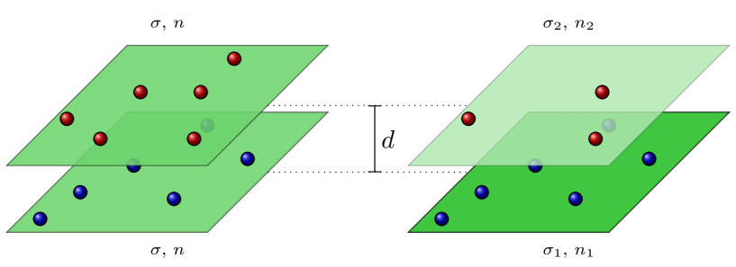
Figure 1: (color online) Schematic views of the Wigner bilayer model. Red (blue) particles form (possibly ordered) lattices on the two parallel plates. Left panel: symmetric case, where both plates carry the same charge density (i.e., $\sigma_{1}=\sigma_{2}$); they are occupied by the same number of particles and thus have both the same particle density (i.e., $n_{1}=n_{2}$). Right panel: asymmetric case, with $\sigma_{1}>\sigma_{2}$ and in general, $n_{1}\neq n_{2}$.

II.2 Symmetric case ($A=1$): structures I through V

Before discussing the results obtained for the asymmetric Wigner bilayers in Sections III to VI, we start by summarizing the results obtained for the symmetric case GoPe96 ; Weis:01 ; messina_2003 ; LoNe07 ; OgML09 ; Samaj12_1 ; Samaj12_2 . Here, the availability of highly accurate data, accessible via pure analytic calculations in Refs. Samaj12_1 ; Samaj12_2 , serve as a stringent benchmark for our implementation of the numerical Evolutionary Algorithm code.

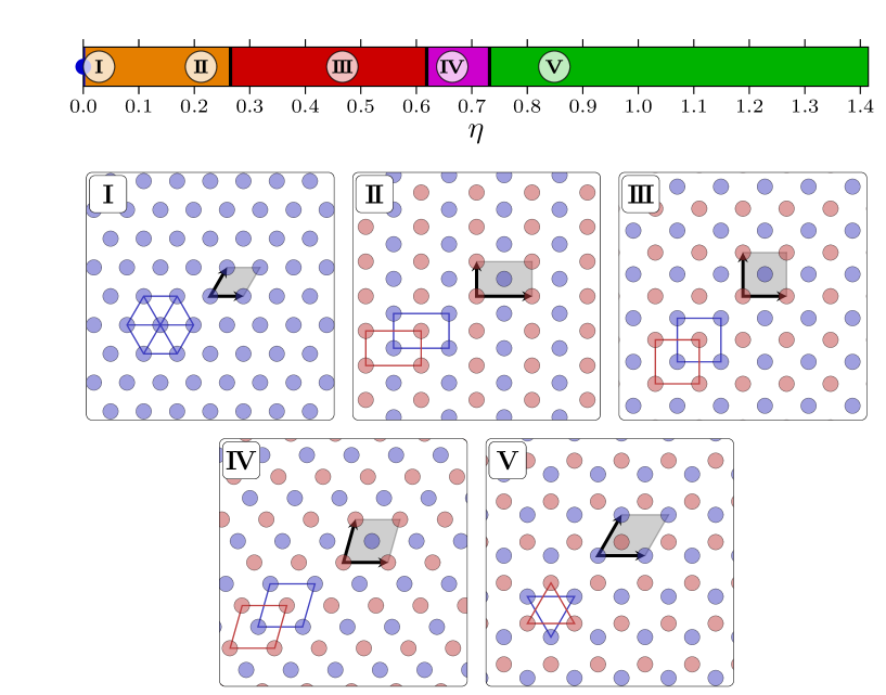
Figure 2: (color online) Symmetric bilayer Wigner system ($A=1$). Top panel: diagram of states in terms of the emerging sequence of structures (I through V) and their respective regions of stability in terms of distance between the plates $\eta$ (as labeled). Structure I is only stable for $\eta=0$ (indicated by a blue dot). Bottom panels: representative snapshots of structures I, II, III, IV, and V (as labeled). Particles in layer 1 are colored blue, particles in layer 2 red. The unit cell of the respective structure is indicated by the shaded area. Blue and red lines highlight interesting structural features in layers 1 and 2, respectively.

For $A=1$, five different structures have been predicted. The top panel of Figure 2 shows their respective regions of stability. For $\eta=0$, the hexagonal monolayer (termed structure I) provides the lowest energy. Phase I can also be viewed as the union of two rectangular lattices where the aspect ratio of its edges, $\Delta$, is given by $\Delta=\sqrt{3}$; the lattices are shifted with respect to each other in both spatial directions by half of the respective side lengths.

As soon as $\eta>0$, the Wigner monolayer is transformed to a staggered rectangular bilayer, the so-called phase II, both rectangular sublattices having the same aspect ratio $\Delta$. There were contentions that the value for the monolayer, i.e., $\Delta=\sqrt{3}$, prevails in a small, but finite $\eta$-range (see, e.g., Refs. GoPe96 ; Weis:01 ; messina_2003 ; OgML09 ). It was shown in Refs. Samaj12_1 ; Samaj12_2 that as soon as $\eta$ is nonzero, $\Delta<\sqrt{3}$, i.e., phase II takes place (see corresponding panel of Figure 2). This phase is stable in the range $0<\eta\lesssim 0.263$ where $\Delta$ decreases continuously to $1$ (corresponding to a square lattice) at $\eta\simeq 0.263$. We can specify structure II via the following set of parameters: $x=1/2$, $\Psi_{4}^{(1,2)}=1$, and $0<\Psi_{6}^{(1,2)}<1$ (for the definition of the bond orientational order parameters $\Psi_{n}^{(\alpha)}$ see Subsection II.6).

At $\eta\simeq 0.263$, structure II transforms via a second-order phase transition Samaj12_1 ; Samaj12_2 into structure III (the staggered square bilayer) which remains stable up to $\eta\simeq 0.621$ (see Figure 2). Structure III can be considered a special case of the neighbouring structures II and IV; thus the transitions $\textrm{I\kern-1.29167ptI}\to\textrm{I\kern-1.29167ptI\kern-1.29167ptI}$ and $\textrm{I\kern-1.29167ptI\kern-1.29167ptI}\to\textrm{I\kern-1.29167ptV}$ are of second order. The critical exponents are of mean-field type Samaj12_1 ; Samaj12_2 , in particular the index $\beta$, which is related to the order parameter takes the mean-field classical value $1/2$. We can define structure III using the set of parameters: $x=1/2$, $\Psi_{4}^{(1,2)}=1$ and $\Psi_{6}^{(1,2)}=0$.

For $0.621\lesssim\eta\lesssim 0.732$, we observe structure IV (see Figure 2), which is a staggered rhombic bilayer. Particles in layer 2 are positioned above the centers of the rhombs in layer 1, and vice versa. The deformation angle $\varphi$ of the rhombs decreases from $\pi/2$ (corresponding to a square and thus to structure III) at $\eta\simeq 0.621$ to a value of $\varphi\simeq 0.386\pi$ at $\eta\simeq 0.732$. We can define structure IV using the following set of parameters: $x=1/2$, $0<\Psi_{4}^{(1,2)}<1$ and $0<\Psi_{6}^{(1,2)}<1$.

Finally, for $0.732\lesssim\eta$, we observe structure V (see the corresponding panel of Figure 2) which is a staggered hexagonal bilayer. Particles in layer 2 are positioned above the centers of equilateral triangles in layer 1, and vice versa. The transition between structures IV and V is of first-order as there is a jump in the deformation angle $\varphi$; simultaneously, particles in each layer move from the center of a rhomb to the projected center of a triangle of the other layer. Since particles form on both layers hexagonal lattices, structure V covers also the asymptotic $\eta\to\infty$ case. We can define structure V using the set of parameters: $x=1/2$, $\Psi_{4}^{(1,2)}=0$ and $\Psi_{6}^{(1,2)}=1$.

II.3 Analytical computations

We establish in Appendix A a connection between the Coulombic energies of systems having the same point-charge configuration on the plates, but otherwise arbitrary surface charges $\sigma_{1}$ and $\sigma_{2}$. Of course, the electroneutrality constraint should be enforced ($\sigma_{1}+\sigma_{2}=n_{1}+n_{2}$). The resulting expression, Eq. (74), will prove useful in Subsection II.4. We also provide here relevant information on the analytical method used to work out Coulombic energies. It follows the periodic lattice summation idea introduced for periodic structures in Refs. Samaj12_1 ; Samaj12_2 . The starting point is the $\Gamma$-identity for the $1/r$ potential

$$\frac{1}{|{\bf r}|}\equiv\frac{1}{\sqrt{r^{2}}}=\frac{1}{\sqrt{\pi}}\int_{0}^{\infty}\frac{dt}{\sqrt{t}}e^{-r^{2}t}$$ (7)

which enables one to transform a lattice Coulomb summation into an integral over the products of two Jacobi theta functions with zero argument, namely

$$\theta_{2}(q)=\sum_{j=-\infty}^{\infty}q^{(j-\frac{1}{2})^{2}},\qquad\theta_{3}(q)=\sum_{j=-\infty}^{\infty}q^{j^{2}},\qquad\theta_{4}(q)=\sum_{j=-\infty}^{\infty}(-1)^{j}q^{j^{2}}.$$ (8)

The neutralizing background subtracts the $q\to 1$ singularities of the product of theta functions. Using a sequence of integral transformations combined with the Poisson summation formula

$$\sum_{j=-\infty}^{\infty}{\rm e}^{-(j+\phi)^{2}t}=\sqrt{\frac{\pi}{t}}\sum_{j=-\infty}^{\infty}{\rm e}^{2\pi{\rm i}j\phi}{\rm e}^{-(\pi j)^{2}/t}$$ (9)

and specific properties of the Jacobi theta functions, the expression for the Coulomb lattice sum can be converted into a quickly converging series of special functions

$$z_{\nu}(x,y)=\int_{0}^{1/\pi}\frac{{\rm d}t}{t^{\nu}}{\rm e}^{-xt}{\rm e}^{-y/t},\qquad y>0,$$ (10)

which are generalizations of the so-called Misra functions Misra . In numerical calculations, the truncation of the generalized Misra series at the fourth term ensures an accuracy of the energy calculations for approximately 17 significant decimal digits.

Near a critical point, the Misra functions can be expanded in powers of the corresponding order parameter; in this way one derives an exact Landau form of the ground state energy. The critical point can thus be specified up to an arbitrary accuracy as a nullity condition for a coefficient and the critical exponents (usually of mean-field type) can be determined. Thus, the above Jacobi-Misra reformulation is not only useful for computing numerically energies, but also to obtain explicit analytical results.

In real lattice structures with particles on both plates, there exist vacancies due to a particle skip from one plate to the other. They cause local deformations of ideal structures which are negligible if the plates are close to one another, but can be considerable at large distances between the plates. In the analytical approach, we ignore these local deformations and consider instead of real structures their idealized simplifications with a reasonable number of particles per unit cell. It is worthwhile to point out that this neglect leads to only small differences in comparison with numerical approaches which deal with realistic, deformed structures.

The analytical approach works well also in special regions of the $(\eta,A)$-plane where the numerical methods fail. A typical example is the region of large distances $\eta$ where the interlayer energy is too small to be detected numerically, while the analytical treatment is able to predict the asymptotic form of the energy and the asymptotic behavior of the occupation parameter.

II.4 Evolutionary Algorithms (EAs)

To identify the ordered ground state configurations of our system, we use an optimization tool based on ideas of Evolutionary Algorithms (EAs) Gottwald:05 . EAs are heuristic approaches to search for global minima in high dimensional spaces Gol89 that are characterized by rugged energy landscapes. We introduce a unit cell which creates (together with its periodic images) a system of infinite extent. The periodic boundary conditions are in compliance with the Ewald summation technique (see Appendix B). Inside this cell, the particles are located in such a way as to minimize the energy of the system, which is a lattice sum.

We initialize the algorithm by creating a set of random particle arrangements. These configurations are graded by their fitness value, a quantity that provides information on how suitable this configuration is to solve the optimization problem. Since we are interested in finding ground state structures, a high fitness value of a particular configuration corresponds to a low value of the energy per particle. We then iteratively use existing configurations to create new ones by applying alternatively one of two operations: crossover and mutation. In the former one we first select two configurations where this choice is biased by high fitness values of the two configurations. Traits of both particle arrangements (such as lattice vectors and/or particle positions) are then combined to form a new configuration. The mutation operation, on the other hand, introduces random changes to a randomly chosen configuration, such as moving an arbitrarily chosen particle or distorting the lattice by changing the underlying vectors. Typically 2000 iterations are required for a particular state point until proper convergence towards the minimum has been achieved.

Our implementation of EAs is memetic, i.e., we combine global and local search techniques: every time a new configuration has been created with one of the two above mentioned EA operations, we apply the L-BFGS-B Byrd:95 algorithm which guides us to the nearest local minimum. As all configurations obtained in this way are local minima, our implementation is similar to basin-hopping techniques Wales:97 .

So far, the method has been applied to a broad variety of systems Fornleitner:08 ; Fornleitner:08a ; Pauschenwein:08 ; Doppelbauer:10 ; Doppelbauer:12 where it has been demonstrated that the concept is able to deal successfully with strongly rugged energy surfaces in high dimensional search spaces. The current application of EAs represents the so far most challenging one, as competing structures are characterized by extremely small energy differences.

We consider unit cells whose size ranges between one and 40 particles, the latter value being imposed by computational limitations. In an effort to find the optimized particle configuration we proceed as follows:

• We do not allow particles to move from one layer to the other and consider all possible values of $x~{}(\leq 0.5)$ that are compatible with the number of particles per cell; according to our experience, this strategy improves the convergence speed when sampling the search space.

• We then fix $A=0$ and perform computations for 201 evenly-spaced values of $\eta\in[0,\sqrt{2}]$; this range in $A$ and $\eta$ covers the most essential features of our system. We thus obtain the optimized energy-values $E(\eta,A=0;x)$.

• We then proceed to $A>0$ and vary this quantity on a grid of 201 evenly-spaced values of $A\in[0,1]$. The optimized energy for these configurations $E(\eta,A;x)$ is then obtained by exploiting the $A$-dependence specified in Eq. (74). The same result is obtained by exploiting the $A$-dependence of the last two terms in Eq. (79) of Appendix B.

For given distance $\eta$ and asymmetry parameter $A$, $E(\eta,A;x)$ is minimized over occupation ratio $x$. For a closer investigation of certain transitions between minima, we employ a related Energy Minimization (EM) approach: here we construct starting configurations suggested by the analytical approach (see Subsection II.3) and then locally optimize the particle positions using the L-BFGS-B Byrd:95 algorithm. This strategy allows us to study specific problems on a considerably finer grid in phase space and to increase, concomitantly, the size of the unit cell to up to 101 particles.

II.5 Bond orientational order parameters

The overall structure and the local particle arrangements realized on each plates are quantified via different types of bond orientational order parameters (BOOPs) Steinhardt:83 ; Mazars:08 . Here, the neighbors of a tagged particle (carrying index $i$) that populate the same layer are identified via a Voronoi construction Voronoi:Book ; the number of nearest neighbors of particle $i$ is denoted by $N_{i}$. Some examples for Voronoi constructions for selected configurations obtained in MC simulations will be shown later.

For the data originating from MC simulations, the average values of BOOPs (i.e., averaged along the MC run) are defined by

$$\langle\Psi_{n}^{(\alpha)}\rangle=\frac{1}{N_{L}}\Big{<}\mbox{\LARGE$\mid$}\sum_{i\in{L}}\frac{1}{N_{i}}\sum_{j=1}^{N_{i}}W_{ij}\exp(in\theta_{ij})\mbox{\LARGE$\mid$}\Big{>};$$ (11)

the tagged particle (with index $i$) is taken from a layer (or from layers) $L$ (as specified via the index $\alpha$ – see below), which hosts in total $N_{L}$ particles; $\theta_{ij}$ is the angle enclosed by the projection of the interparticle vector ${\bf r}_{ij}$ onto one of the planes and an arbitrary, but fixed direction, and $W_{ij}$ is a weight introduced in Mickel:13 used to appreciate correctly the length of the sides of the Voronoi cells of a given particle $i$; to be more specific, $W_{ij}$ is computed via

$$W_{ij}=\frac{l_{j}}{\sum_{k=1}^{N_{i}}l_{k}}$$ (12)

where $l_{j}$ the length of the side of the Voronoi cell that separates particle $i$ from its neighbor $j$. The index $n$, appearing in the definition of the $\langle\Psi_{n}^{(\alpha)}\rangle$ is an integer: we have computed BOOPs for $n=4,5,6,7,8,10,12,18$ and 24 both in EA and MC calculations. Finally, the superscript $\alpha$ refers to the four different methods of Voronoi construction that we have used for calculating the BOOPs: for layer 1 ($\alpha=1$), for layer 2 ($\alpha=2$), or for all particles after projecting them onto the same plane ($\alpha=3$); in addition, we have also calculated modified BOOPs ($\alpha=4$), which quantify the geometry of “holes”, i.e., of particles in layer 2 and the surrounding particles in layer 1.

The Voronoi constructions allows to estimate the (averaged) distribution of the number of neighbors for particles in each layer Leipold:15 ; we denote the probability (as calculated from the MC simulations) that a particle has $n$ neighbours in layer $\alpha$ by $p_{\alpha}(n)$.

II.6 Monte Carlo simulations

In the calculations based on the analytical approach and on the EA, the exploration of the diagram of states in the $(\eta,A)$-plane is limited to a rather small number of particles within the primitive cells (i.e., to $N\leq 40$). However, some of the EA based calculations have revealed that crystal phases with a rather large number of particles per primitive cell can exist. To provide an estimate of the stability of the ordered structures predicted by the EA investigations, we have performed Monte Carlo (MC) simulations at finite, but small temperatures and for considerably larger systems (typically $N\sim 4000$). These simulations are carried out in the canonical ensemble, assuming a variable shape of the simulation box ${\cal S}_{0}$ (but assuming a fixed surface area $S$). Trial moves for the shape of the box in combination with the Ewald method Mazars:11 are documented in Ref. Weis:01 ; this method is particularly well suited to study solid-solid and solid-liquid transitions and has been successfully applied for the study of the crystal phases of Coulomb Weis:01 and Yukawa bilayers Mazars:08 .

For $\eta=0$, our system is equivalent to a one-component plasma confined to a plane (OCP-2D); for this system the ground state is a triangular lattice (corresponding to our structure I). The only relevant thermodynamic variable that characterizes the OCP-2D system is the coupling constant $\Gamma$, defined via $\Gamma=e^{2}\sqrt{\pi(\sigma_{1}+\sigma_{2})}/(k_{\rm B}T)$, $k_{\rm B}$ being the Boltzmann constant. Melting of structure I of the OCP-2D system occurs at $\Gamma\simeq 140$ Mazars:15 . In an effort to remain as close to the ground state of the bilayer as possible, we have chosen in all MC simulations of the present study the temperature such that $1500\lesssim\Gamma\lesssim 2200$.

We define a MC-cycle as $N$ trial moves of randomly chosen particles and a trial change of the shape of the simulation box. A trial move of a particle is realized either as spatial displacement within the layer the particle belongs to (in 90 - 97 percent of the cases) or as a trial move of this particle from one layer to the other (in the remaining 3 - 10 percent of the cases). Equilibration is realized during $0.3-1.6~{}10^{6}$ MC-cycles; subsequently ensemble averages are taken over $0.3-1.0~{}10^{6}$ MC-cycles rque20 .

In a first set of simulations we have used as initial configurations those particle arrangements that have either been identified in preceding EA runs, or ordered structures found for the symmetric bilayer ($A=1$), or random particle configurations. However, since for the first case the number of particles per primitive cell, $N$, can differ substantially between two neighboring state points, it is difficult to observe transitions between two ordered structures in MC simulations when some fixed value of $N$ is assumed a priori. To overcome this problem, we have considered specific sets of systems for which the ordered structures are throughout compatible with the number of particles used in the MC simulations: to this end we have performed simulations for states that populate domains in the ($\eta,A$)-plane where the value of $x=N_{2}/N$ is essentially constant. In Figure 3, we highlight a few of these domains as they are predicted via the EA-based approach. They are characterized by a fixed rational value of $x$, the largest of these regions are found to be those characterized by $x=$ 3/7, 1/3, 1/4 and 1/5.

Since the ordered structures that populate the ($x=1/2$)-domain are identical to those that have been identified for the symmetric bilayer (cf. discussion in Subsection II.2), we have focused in our MC simulations on domains specified by $x<1/2$; to be more specific, we discuss in Section VII and in the Appendix F results obtained for four selected $x$-values. In an effort to explore these regions systematically, we have defined for each of them in an empiric manner simple polynomial curves, $A_{x={\rm const.}}(\eta)$, which define within numerical accuracy pathways through these domains; the expressions for these polynomials are collected for the different domains in Appendix F.

The state points that have been investigated with MC simulations along these curves are marked by symbols in Figure 3. For each of these four pathways an (ordered) initial configuration has been chosen according to the predictions of the EA approach for this specific state point (highlighted by a red triangle in Figure 3). This particular configuration then served as a starting configuration for all the other states located along the corresponding line of constant $x$.

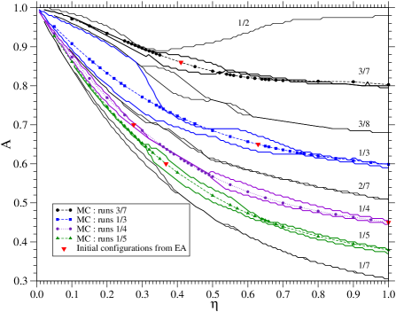
Figure 3: (color online) Domains in the $(\eta,A)$-plane where – according to the EA predictions – the value of $x=N_{2}/N$ is constant; regions for eight selected $x$-values are shown (as labeled). The dotted lines are simple polynomial fits $A=A(\eta)$ which pass within numerical accuracy through the respective regions of constant $x$. The red triangles represent on each of these curves those states which were used as initial configurations (predicted by EA calculations) of the subsequent MC runs of all the other states, located along these lines (marked by the colored dots).

Additional structural information can be extracted from MC simulations via the intra- and inter-layer pair correlation functions, respectively defined via

$$g_{\alpha}(s) = \frac{1}{4\pi}\frac{1}{s\sigma_{\alpha}(N_{\alpha}-1)}{\Big{<}}\sum_{i\in L_{\alpha}}\sum_{\begin{subarray}{c}j\in L_{\alpha}\\ j\neq i\end{subarray}}\delta(s-\mid{\bf s}_{ij}\mid){\Big{>}}~{}~{}~{}~{}~{}\alpha=1,2$$ (13)

$$g_{3}(s) = \frac{1}{2\pi}\frac{1}{s\sigma_{1}\sigma_{2}S}{\Big{<}}\sum_{i\in L_{1}}\sum_{j\in L_{2}}\delta(s-\mid{\bf s}_{ij}\mid){\Big{>}}.$$

Here ${\bf s}_{ij}$ represents the vector between particles $i$ and $j$ and $N_{\alpha}$ ($\alpha=1,2$) is the number of particles in layer $\alpha$. In an effort to capture the long-range orientational order, we have also computed the bond orientational correlation function for each layer $\alpha$ via

$$G_{n,\alpha}(s)=\frac{1}{g_{\alpha}(s)}\Big{<}\Psi^{(\alpha)}_{n}(0)\Psi^{(\alpha)}_{n}(s)\Big{>}~{}~{}~{}~{}~{}\alpha=1,2,3~{}~{}~{}~{}~{}n~{}{\rm integer.}$$ (14)

If $\langle\Psi_{n}^{(\alpha)}\rangle\neq 0$, a long-range orientational order can be identified via the bond orientational correlation functions $G_{n,\alpha}(s)$, which then fulfill the relation

$$\lim_{s\rightarrow\infty}G_{n,\alpha}(s)=\langle|\Psi_{n}^{(\alpha)}|^{2}\rangle.$$ (15)

III Structural informations and taxonomy

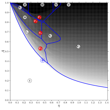
Figure 6: (color online) Same as Fig. 5, now in terms of the order parameter $x=n_{2}/n$. The following gray-scale encoding was used: $x=0$ corresponds to white, $x=1/2$ to black. Note that the value $x=1/3$ is of particular relevance (see regions surrounding the labels of structures H, $\textrm{S}_{2}$, and $\textrm{S}_{1}$).

Structural informations are compiled in the different diagrams of state of Figures 4 to 6. Covering a representative range of the $(\eta,A)$-plane, these figures highlight on one hand those regions where the analytical approach predicts the stability of the emerging structures; these areas are specified by the respective labels and are delimited by solid curves. On the other hand, these figures provide on a pixel-based presentation information about the results obtained via the EA approach; each of the $\sim$ 35000 pixels contain via a color- or a shade-code the structural information for the respective state point: these encoding schemes were either based on the BOOPs (Fig. 4), the number of particles per unit cell (Fig. 5), or the occupation fraction $x$ (Fig. 6). In particular the BOOPs (in combination with $x$) played a central and indispensable role in identifying the ordered ground state configurations (see below). Panels of Fig. 4 are constructed by assigning to each pixel a color depending on the values of the BOOPs (see the caption).

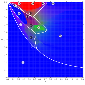
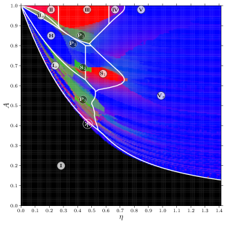
Figure 4: (color online) Diagrams of states in the $(\eta,A)$-plane in terms of the BOOPs. Each pixel (corresponding to a state point) is assigned a color, which is based on the respective values of the specific parameters of the respective ground state configuration: within this $\Psi$RGB-color scheme, the value of $\langle\Psi_{4}^{(\alpha)}\rangle$ sets the red-component, the value of $\langle\Psi_{5}^{(\alpha)}\rangle$ sets the green-component, and the value of $\langle\Psi_{6}^{(\alpha)}\rangle$ sets the blue-component. Top left panel: order parameters $\langle\Psi^{(1)}\rangle$ for layer 1; top right panel: order parameters $\langle\Psi^{(2)}\rangle$ for layer 2. Bottom left panel: $\langle\Psi^{(3)}\rangle$ involving both layers; bottom right panel: $\langle\Psi^{(4)}\rangle$ based on the geometry of “holes”; for the respective definitions of the BOOPs see Subsection II.5. White lines mark regions where the analytical approach predicts the stability of the respective structure (as labeled). Particle arrangements marked by dark labels are too complicated to be amenable to the analytical approach. The white star marks a bi-critical point (see text).

In our investigations, the numerical and the analytical approaches are complementary in the following sense: (i) the EA-based optimization methods suggested particle arrangements that have been further analyzed with the analytical approach; (ii) results based on the latter method represented a stringent test for the data obtained via the EA route. The EA-based part of the studies has been carried out for approximately 35000 state points: for each of them the number of particles per unit cell was systematically increased from simple lattices to cells with up to 40 basis particles. As a consequence the numerical resolution in $x$ in the EA approach is limited: in particular, the largest value for $x<1/2$ that can be obtained is $x=19/39=0.487$. Thus it cannot be excluded that significantly larger unit cells could allow for a more complicated two-dimensional particle arrangement which might be energetically more favourable. The analytical framework uses the simplifying assumption that the competing structures on both plates are undistorted (i.e., ideal). The colored region, in contrast, covers data obtained via the numerical approach which is able to grasp appropriately the emerging minute deviations of the particle configurations from ideal lattices. The mentioned limitations of the analytical approach explain small discrepancies between the limiting white curves and the border of the colored region.

When identifying ordered structures, we first classify particle arrangements by the respective value of $x$. Then, further refinement is achieved by a classification scheme, involving one or more BOOPs $\langle\Psi_{n}^{(\alpha)}\rangle$. The relevant criteria for identifying structures in the EA approach are summarized in Table 1. While the detailed discussion of the emerging structures is postponed to the following sections, a few general remarks are in order:

• the relatively large regions of uniform and pure colors (i.e., red, green, or blue) occurring in the panels for the BOOPs $\langle\Psi^{(1)}_{n}\rangle$ and $\langle\Psi^{(2)}_{n}\rangle$ in Fig. 4 for most of the state points investigated indicate that the particles form simple, ordered structures with four-, five-, or six-fold symmetry in the respective layers;

• the degree of structural commensurability of the two sublattices in the two layers is reflected by the respective colors encoded in the values of $\langle\Psi^{(3)}_{n}\rangle$ and $\langle\Psi^{(4)}_{n}\rangle$: the effort of the system to guarantee a high degree of structural commensurability leads to pure colors of the respective state points; this is for instance the case along the stripe-shaped regions in the domain where the structure $\textrm{V}_{x}$ is stable: within each of these stripes the value $x$ is essentially constant;

• related observations can also be made for the shade-coded plot of $N$, the number of particles per unit cell (Fig. 5). The white/bright regions characterize state points with a simple, ordered structure (i.e., with only a few particles per unit cell) and a high degree of commensurability between the two sub-structures. This also holds for the stripe-shaped regions (along which $x$ is essentially constant) located within the domain where structure $\textrm{V}_{x}$ is stable. In contrast, large $N$ values (i.e. dark regions in Fig. 5) indicate the occurrence of complex, incommensurate structures.

Table 1: Classification scheme used to identify the observed ordered structures (first and last columns) in the asymmetric Wigner bilayer system, based on their respective values of $x$ (second column) and of the BOOPs (third column): the first criterion is the value of $x$; then, further refinement is achieved by using BOOPs or linear combinations thereof. Note that the threshold values for the BOOPs (specified in the third column) are to some extent arbitrary. For convenience, we have dropped the symbols that indicate the averaged values of the BOOPs (i.e., $\Psi^{(\alpha)}_{n}$ stands for $\langle\Psi^{(\alpha)}_{n}\rangle$). The occupation index $x$ is defined in Eq. (5).

I	$x=0$		hexagonal monolayer
II	$x=1/2$	$\Psi_{4}^{(1,2)}=1$, $0<\Psi_{6}^{(1,2)}<1$	rectangular bilayer
III	$x=1/2$	$\Psi_{4}^{(1,2)}=1$, $\Psi_{6}^{(1,2)}=0$	square bilayer
IV	$x=1/2$	$0<\Psi_{4}^{(1,2)}<1$, $0<\Psi_{6}^{(1,2)}<1$	rhombic bilayer
V	$x=1/2$	$\Psi_{4}^{(1,2)}=0$, $\Psi_{6}^{(1,2)}=1$	hexagonal bilayer
$\textrm{I}_{x}$	$0<x<1/3$	$0.9<\Psi_{6}^{(3)}$
H	$x=1/3$	$0.9<\Psi_{6}^{(3)}$	honeycomb (layer 2)
$\textrm{I\kern-1.29167ptI}_{x}$	$1/3<x<1/2$	$0.9<\Psi_{6}^{(3)}$
$\textrm{V}_{x}$	$0<x<x^{*}$	$0.9<(1-x)\Psi_{6}^{(1)}+x\Psi_{6}^{(2)}$	hexagonal bilayer
$\textrm{DV}_{x}$	$2/5\leq x<1/2$	$0.5\leq\Psi_{6}^{(1,2)}$, $\Psi_{4}^{(1)}\sim 0.4$, $\Psi_{5}^{(2)}\sim 0.3$	distorted hexagons
$\textrm{S}_{1}$	$x=1/3$	$0.9<\Psi_{5}^{(1)}$, $0.9<\Psi_{4}^{(2)}$	snub square (layer 1)
$\textrm{S}_{2}$	$x=1/3$	$0.45<\Psi_{5}^{(2)}$	snub square (layer 2)
P-type	$1/3<x<1/2$	$0.45<\Psi_{5}^{(2)}$	pentagonal in layer 2
	or $0<x<1/3$	or $0.9<\Psi_{5}^{(4)}$	pentagonal holes

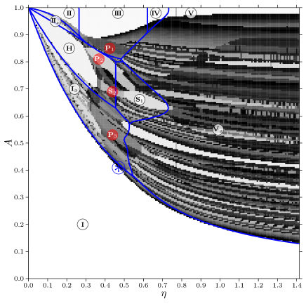
Figure 5: (color online) Diagram of states in terms of numbers of particles per unit cell ($N$), as obtained via the EA-based approach. The following gray-scale encoding was used: $N=2$ corresponds to white, $N=40$ to black. Simple structures that are easily tractable with the analytical approach (specified by bright labels, with their respective regions of stability delimited by blue lines) appear thus as bright regions. Structure $\textrm{V}_{x}$ represents an exception to this rule, since for this case the structures of the two layers are not necessarily strongly correlated. Structures with red-colored labels are too complicated to be amenable to the analytical approach. The blue star marks a bi-critical point (see text).

IV Structures emerging at small $\eta$: I, $\textrm{I}_{x}$, H, and $\textrm{I\kern-1.29167ptI}_{x}$

IV.1 Phase I

When the two plates are at contact ($\eta=0$), the lowest energy of the system corresponds to the hexagonal Wigner monolayer (structure I). Each of the triangles is shared by three particles and each particle is surrounded by six triangles; hence, there are just $6\times 1/3=2$ triangles per particle. Therefore the lattice spacing $a$ is imposed by the requirement of electro-neutrality as $\sqrt{3}\,a^{2}(\sigma_{1}+\sigma_{2})=2$ . The hexagonal lattice can be considered as the union of two rectangular lattices with the aspect ratio $\Delta=a_{2}/a_{1}=\sqrt{3}$, shifted with respect to each other in both spatial directions by half of the respective side lengths. Since for $\eta=0$, the monolayer is neutral by definition, we find – using the formalism developed in Appendix A – for the energy $E_{\textrm{I}}(\eta=0)=E_{pp}^{\rm neutr}$, where

$$\frac{E_{pp}^{\rm neutr}}{N}=\sum_{(j,k)\neq(0,0)}\frac{e^{2}}{2a\sqrt{j^{2}+3k^{2}}}+\sum_{j,k}\frac{e^{2}}{2a\sqrt{(j+1/2)^{2}+3(k+1/2)^{2}}}-\mbox{backgr.}$$ (16)

Here, the lattice Coulomb summations extend over all integers; infinite constants in the summations are regularized by the neutralizing background. We define the Madelung structural constant $c$ of the hexagonal lattice in the following way

$$c\equiv\frac{E_{\textrm{I}}(\eta=0)}{Ne^{2}\sqrt{\sigma_{1}+\sigma_{2}}}.$$ (17)

Using the technique put forward in Refs. Samaj12_1 ; Samaj12_2 , the lattice Coulomb summations can be transformed into integrals over the Jacobi theta functions with zero argument (8). In terms of the function

$$c(\Delta)\equiv\frac{1}{2^{3/2}\sqrt{\pi}}\int_{0}^{\infty}\frac{{\rm d}t}{\sqrt{t}}\left\{\left[\theta_{3}({\rm e}^{-\Delta t})\theta_{3}({\rm e}^{-t/\Delta})-1-\frac{\pi}{t}\right]+\left[\theta_{2}({\rm e}^{-\Delta t})\theta_{2}({\rm e}^{-t/\Delta})-\frac{\pi}{t}\right]\right\},$$ (18)

the Madelung constant is given by $c=c(\sqrt{3})$. The neutralizing background subtracts the ($t\to 0$)-singularities $\pi/t$ of the products of two $\theta_{3}$- and two $\theta_{2}$-functions. Based on results of Refs. Samaj12_1 ; Samaj12_2 , the expression for $c$ can be transformed into a quickly converging series of the generalized Misra functions (10) and we obtain the well-known value $c=-1.960515789\ldots$ .

For $A<1$ and at sufficiently small distances $\eta$ between the plates, all particles forming the hexagonal Wigner crystal will remain at their positions on plate 1; such a monolayer phase will also be coined as phase I. Since $x=0$ in phase I, the corresponding energy is given – according to the “neutralization” analysis of Appendix A – by expression (72) as follows

$$\frac{E_{\textrm{I}}(\eta,A)}{Ne^{2}\sqrt{\sigma_{1}+\sigma_{2}}}=c+2^{3/2}\pi\eta\left(\frac{A}{1+A}\right)^{2}.$$ (19)

Whether or not phase I is stable can be tested qualitatively by moving one of the particles perpendicularly from plate 1 at $z=0$ to plate 2 at $z=d$. This move is accompanied by the increase of the potential energy of the particle by

$$\Delta E_{\rm pot}=-e\left[\phi(d)-\phi(0)\right]=2\pi e^{2}(\sigma_{1}-\sigma_{2})d.$$ (20)

Simultaneously, since the distance of the reference particle to all other particles is increased, its interaction energy is decreased by $\Delta E_{\rm int}\sim-e^{2}Cd^{2}$ ($C>0$ being a structure constant of the hexagonal Wigner lattice) due to the symmetry $[z\to-z]$ of the interaction potential. As soon as $A<1$, the total energy change of this operation

$$\Delta E=\Delta E_{\rm pot}+\Delta E_{\rm int}\sim e^{2}[2\pi(\sigma_{1}-\sigma_{2})d-Cd^{2}]$$ (21)

is dominated by the linear potential term for small $d$. $\Delta E$ is therefore positive and the particle prefers to remain in its lattice position within phase I. Since we proceed here by necessary condition for stability, this provides a hint that phase I is always stable at sufficiently small distances.

The way of how the monolayer phase I transforms into another bilayer phase at a specific distance $d_{c}$ (or, equivalently, $\eta_{c}$) depends on the value of the asymmetry parameter $A$; these values form in the diagram of states the line $\eta_{c}(A)$, or, equivalently, $A_{c}(\eta)$. Two scenarios will be discussed in the following: one valid for $A$ close to 1 where $d_{c}$ is small and the transition is due to the perpendicular moves of particles from plate 1 to plate 2 and the other for small $A$, where $d_{c}$ is somewhat larger. In the latter case, the moves of the particles from plate 1 in Structure I to plate 2 to form the ground state are in a direction that is no longer perpendicular to the plates.

IV.2 Phase $\textrm{I}_{x}$

Starting from the monolayer, keeping $A$ fixed to a value close to unity and increasing $\eta$, more and more charges will shift their location to layer 2: they leave distorted hexagonal holes in layer 1 and form, in turn, a new, ordered particle arrangement in layer 2. This is the origin of the so-called family of structures I_x. To be more specific, phase I_x can be defined as a bilayer structure where the projections of the particles of both layers onto one plane form a hexagonal phase (which can be slightly distorted). The parameter $x=N_{2}/N$ specifies the number of particles that have been shifted in a perpendicular direction from the hexagonal monolayer on plate 1 to plate 2 (see snapshots in Fig. 7).

The essentially unrestricted search of the EA-based optimization algorithm provides evidence that upon increasing distance $\eta$ at a fixed large $A$, structure I_x transforms first into structure H and then into phase II_x (to be discussed in detail in Subsection IV.4). Both of these phases are characterized by the feature that the projected particle positions of both layers form an almost perfect (i.e., possibly slightly distorted) hexagonal lattice; we can characterize this family of structures via the criterion $0.9<\Psi_{6}^{(3)}$ (see Table 1). The difference between these three structures can be quantified via the occupation parameter $x$; the respective ranges of stability are displayed in Fig. 4:

• structure I_x (with a representative snapshot in the left panel of Fig. 7 for $x=1/4$) has $0<x<1/3$;

• structure H (central panel of Fig. 7) is characterized by $x=1/3$ and can be considered as a special case of both neighbouring structures, i.e., of I_x and II_x; structure H consists of a honeycomb lattice in layer 1 and a hexagonal lattice in layer 2 where particles of the latter are located above the centers of the hexagonal rings in layer 1;

• eventually, structure II_x (see right panel of Fig. 7), having $1/3<x<1/2$.

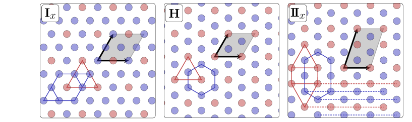
Figure 7: (color online) Representative snapshots of structures $\textrm{I}_{x}$, H, and $\textrm{I\kern-1.29167ptI}_{x}$ (see text). Particles in layer 1 are colored blue, particles in layer 2 red. The unit cell of the respective structure is indicated by the shaded area. Blue and red lines highlight interesting structural features in layers 1 and 2, respectively. For the dotted, colored lines see text. Left panel: structure $\textrm{I}_{x}$ emerging for $\eta=0.184$ and $A=0.775$, with $x=1/4$. Center panel: a special case of structure $\textrm{I}_{x}$, H, for $\eta=0.198$ and $A=0.85$, with $x=1/3$. Right panel: structure $\textrm{I\kern-1.29167ptI}_{x}$ for $\eta=0.148$ and $A=0.95$, with $x=2/5$.

Within the analytic approach it is not possible to fully capture the features of all the emerging phases, as $x$ is essentially continuous. With a reasonable amount of computational effort the analytic route is able to grasp those I_x phases, where the two sublattices (with lattice spacings $a$ and $b$, respectively) are commensurate hexagonal layers. These lattices form a limited subset of the whole structural family I_x, where the corresponding values of $x$ are restricted to a subset of $\mathbb{Q}$, as detailed in the following. To specify the possible values of $b/a$ (with $b>a$), which guarantee commensurability of the two sublattices on plates 1 and 2, we notice that joining two arbitrary vertices of lattice $\alpha$ implies a side of the hexagonal lattice $\beta$ whose all points also belong to $\alpha$. The primitive vectors of the hexagonal lattice $\alpha$ are

$${\bf a}_{1}=a(1,0),\qquad{\bf a}_{2}=\frac{a}{2}(1,\sqrt{3}).$$ (22)

Choosing the lattice vector of sublattice $\beta$ as ${\bf b}=j{\bf a_{1}}+k{\bf a}_{2}$ with $(j,k)$ two arbitrary positive integers such that $j+k\neq 0,1$ [i.e., $(j,k)=(0,2)$, $(1,1)$, $(0,3)$, $(1,2)$, $(0,4)$, $(1,3)$, $(2,2)$, etc.] we find that $b^{2}=a^{2}(j^{2}+jk+k^{2})$. Since $S/N_{2}=\sqrt{3}b^{2}/2$, the possible values of $x$ are constrained to

$$x\equiv\frac{N_{2}}{N}=\frac{a^{2}}{b^{2}}=\frac{1}{j^{2}+jk+k^{2}},\qquad x\in\left\{\frac{1}{3},\frac{1}{4},\frac{1}{7},\frac{1}{9},\frac{1}{12},\frac{1}{13},\frac{1}{16},\ldots\right\}.$$ (23)

The admissible discrete values of the occupation parameter $x$ become essentially dense when $x\to 0$ and we can take $x$ as a quasi-continuous variable in that limit.

Among the structures $\textrm{I}_{x}$ the one with the largest occupation parameter, namely $x=1/3$, is pictured in the center panel of Fig. 7; it is the aforementioned structure H. Structure H has a special property: due to a high degree of symmetry of the internal architecture, no local distortions of the two sublattices on plates 1 and 2 can be observed. Therefore analytical results match perfectly the numerical data of EA-based method. This particularly stable internal architecture guarantees a relatively large region of the parameter space $(\eta,A)$ over which this phase represents the energetically most favorable candidate.

IV.3 Transition $\textrm{I}\to\textrm{I}_{x}$

Whether the system remains in its monolayer configuration I or populates the second layer (leading thus to structure $\textrm{I}_{x}$) is of course the result of an energetic competition, to which the analytical approach has – despite the above mentioned limitations – essentially full access. Let a reference particle 1 be located on sublattice $\alpha$ of plate 1. The occurring energy change of phase $\textrm{I}_{x}$ with respect to phase I is given by

$$\frac{E_{\textrm{I}_{x}}(\eta,A;x)-E_{\rm I}(\eta,A)}{e^{2}N_{2}} = 2\pi(\sigma_{1}-\sigma_{2})d+\sum_{j\in\alpha\atop j\neq 1}\left(\frac{1}{\sqrt{R_{1j}^{2}+d^{2}}}-\frac{1}{R_{1j}}\right)$$ (24)

$$-\sum_{j\in\beta}\left(\frac{1}{\sqrt{R_{1j}^{2}+d^{2}}}-\frac{1}{R_{1j}}\right).$$

The first term on the rhs of this equation corresponds to the increase of the potential energy by taking $N_{2}$ particles from plate 1 to 2. The second term is the change in the interaction energy of a particle transferred from plate 1 to 2, with respect to particles remaining in sublattice $\alpha$. The particles located in sublattice $\beta$ should not be included in that sum as the mutual interaction energy of particles in sublattice $\beta$ is unchanged by their simultaneous transfer to plate 2, so the third term in the above relation is simply the compensation sum.

Using methods outlined in Refs. Samaj12_1 ; Samaj12_2 , we obtain the following integral representation of the energy change, specified in Eq. (24):

$$\frac{E_{\textrm{I}_{x}}(\eta,A;x)-E_{\textrm{I}}(\eta,A)}{e^{2}N\sqrt{\sigma_{1}+\sigma_{2}}}=x\Bigg{\{}2^{3/2}\pi\frac{1-A}{1+A}\eta\phantom{aaaaaaaaaaaaaaaaaaaaaaaaaaaaaaaaaaa}$$

$$-\frac{1}{\sqrt{2\pi}}\int_{0}^{\infty}\frac{{\rm d}t}{\sqrt{t}}\left(1-{\rm e}^{-\eta^{2}t}\right)\left[\theta_{3}({\rm e}^{-\sqrt{3}t})\theta_{3}({\rm e}^{-t/\sqrt{3}})-1+\theta_{2}({\rm e}^{-\sqrt{3}t})\theta_{2}({\rm e}^{-t/\sqrt{3}})\right]$$

$$+\frac{\sqrt{x}}{\sqrt{2\pi}}\int_{0}^{\infty}\frac{{\rm d}t}{\sqrt{t}}\left(1-{\rm e}^{-\eta^{2}xt}\right)\left[\theta_{3}({\rm e}^{-\sqrt{3}t})\theta_{3}({\rm e}^{-t/\sqrt{3}})-1+\theta_{2}({\rm e}^{-\sqrt{3}t})\theta_{2}({\rm e}^{-t/\sqrt{3}})\right]\Bigg{\}}.$$ (25)

The integrals over the Jacobi theta functions are expressible via the $K$-function defined in Eq. (81) of Appendix C as follows:

$$\frac{E_{\textrm{I}_{x}}(\eta;x)-E_{\textrm{I}}(\eta)}{e^{2}N\sqrt{\sigma_{1}+\sigma_{2}}}=\frac{x}{\sqrt{2}}\left[-8\pi\frac{A}{1+A}\eta+4\pi\eta x-K(\sqrt{3},\eta)+\sqrt{x}K(\sqrt{3},\sqrt{x}\eta)\right].$$ (26)

Compared to the expression (19) for the energy of phase I, the energy of phase $\textrm{I}_{x}$ is now given by

$$\frac{E_{\textrm{I}_{x}}(\eta,A;x)}{e^{2}N\sqrt{\sigma_{1}+\sigma_{2}}}=2^{3/2}\pi\eta\left(x-\frac{A}{1+A}\right)^{2}+c+\frac{x}{\sqrt{2}}\left[-K(\sqrt{3},\eta)+\sqrt{x}K(\sqrt{3},\sqrt{x}\eta)\right].$$ (27)

Using the series representation of $K(\sqrt{3},\eta)$ presented in Appendix C, this expression becomes suitable for numerical calculations.

The transition from phase I (with $x=0$) to phase $\textrm{I}_{x}$ (with $x>0$) is continuous, i.e. of second-order (as discussed in the following). In an effort to find a formal anallogy of our system of classical particles at zero temperature with a statistical model at finite temperature, we keep in mind that the role of the inverse temperature is played in our case by the dimensionless distance between the plates $\eta$, while the role of the free energy is played by the energy given in Eq. (25), or equivalently in Eq. (27). The order parameter, which increases from 0 just at the critical point continuously to finite values, is the occupation number $x$.

For small $x$, the expression for the energy (25) can be expanded in powers of $x$ as follows

$$\frac{E_{\textrm{I}_{x}}(\eta,A;x)-E_{\textrm{I}}(\eta,A)}{e^{2}N\sqrt{\sigma_{1}+\sigma_{2}}}\simeq f(\eta)x+\frac{2^{3/2}\pi}{\lambda}\eta^{2}x^{5/2}+O(x^{7/2}),$$ (28)

where

$$f(\eta) = 2^{3/2}\pi\frac{1-A}{1+A}\eta-\frac{1}{\sqrt{2\pi}}\int_{0}^{\infty}\frac{{\rm d}t}{\sqrt{t}}\left(1-{\rm e}^{-\eta^{2}t}\right)\left[\theta_{3}({\rm e}^{-\sqrt{3}t})\theta_{3}({\rm e}^{-t/\sqrt{3}})-1\right.$$ (29)

$$\left.+\theta_{2}({\rm e}^{-\sqrt{3}t})\theta_{2}({\rm e}^{-t/\sqrt{3}})\right];$$

the constant $\lambda$ is defined in Eqs. (32) and (33). Note that the expansion of the energy in the order parameter $x$, given in Eq. (28) is not analytic due to the long-range Coulomb interaction of the charged particles. This feature is in striking contrast to the standard mean-field, Landau-type theory of phase transitions where the thermodynamic potential (in our case the energy), assumed to be a smooth function of the order parameter, is expanded in integer powers of the order parameter, reflecting the symmetry of the system. Our energy change (28) does not show the symmetry invariance with respect to a transformation of $x$, which explains the occurrence of rational powers in the order parameter $x$; we emphasize that our expansion (28) starts with $x$ as the leading term, which is in contrast to the well-known Landau expansions, starting – in the absence of an external field – with a term proportional to $x^{2}$.

The free variable $x$ has to be chosen in such a way that it provides the minimal value of the energy. The extremum condition for $E_{\textrm{I}_{x}}(\eta;x)$, i.e., $\partial_{x}E_{\textrm{I}_{x}}(\eta;x)=0$, when applied to relation (28) takes the form

$$0\simeq f(\eta)+\frac{5\sqrt{2}\pi}{\lambda}\eta^{2}x^{3/2}+O(x^{5/2}).$$ (30)

For a given value of $A$ the critical point $\eta_{c}$ is identified by the condition $f(\eta_{c})=0$, i.e.,

$$4\pi\frac{1-A}{1+A}\eta_{c}=\frac{1}{\sqrt{\pi}}\int_{0}^{\infty}\frac{{\rm d}t}{\sqrt{t}}\left(1-{\rm e}^{-\eta_{c}^{2}t}\right)\left[\theta_{3}({\rm e}^{-\sqrt{3}t})\theta_{3}({\rm e}^{-t/\sqrt{3}})-1+\theta_{2}({\rm e}^{-\sqrt{3}t})\theta_{2}({\rm e}^{-t/\sqrt{3}})\right].$$ (31)

As can be seen in Fig. 4, this analytic estimate of critical points $\eta_{c}=\eta_{c}(A)$ (i.e., the white line that separates phases I and $\textrm{I}_{x}$ and ending at the bi-critical point with the latter one marked by the star) coincides well with the EA results. In the limit $\eta\to 0$ (or, equivalently $A\to 1$), expression (31) reduces to the exact asymptotic relation

$$\eta_{c}(A)\mathop{\sim}_{A\to 1}\lambda\frac{1-A}{1+A},\qquad\lambda=\frac{4\pi}{\frac{1}{\sqrt{\pi}}\int_{0}^{\infty}{\rm d}t\,\sqrt{t}\left[\theta_{3}({\rm e}^{-\sqrt{3}t})\theta_{3}({\rm e}^{-t/\sqrt{3}})-1+\theta_{2}({\rm e}^{-\sqrt{3}t})\theta_{2}({\rm e}^{-t/\sqrt{3}})\right]}.$$ (32)

Using the general theory of lattice sums Zucker_74 ; Zucker_75 it can be shown that

$$\frac{1}{\sqrt{\pi}}\int_{0}^{\infty}{\rm d}t\,\sqrt{t}\left[\theta_{3}({\rm e}^{-\sqrt{3}t})\theta_{3}({\rm e}^{-t/\sqrt{3}})-1+\theta_{2}({\rm e}^{-\sqrt{3}t})\theta_{2}({\rm e}^{-t/\sqrt{3}})\right]$$

$$=3^{1/4}\zeta\left(\frac{3}{2}\right)\left[\zeta\left(\frac{3}{2},\frac{1}{3}\right)-\zeta\left(\frac{3}{2},\frac{2}{3}\right)\right],$$ (33)

where $\zeta(z,q)=\sum_{j=0}^{\infty}1/(q+j)^{z}$ is the generalized Riemann zeta function and $\zeta(z)\equiv\zeta(z,1)$. The prefactor $\lambda\simeq 0.999215$ in Eq. (32) is thus very close, but not equal, to 1.

The function $f(\eta)$ given in Eq. (29) is dominated for small $\eta$ by the linear term, so that $f(\eta)>0$ for $\eta<\eta_{c}$, while $f(\eta)<0$ for $\eta>\eta_{c}$; thus we can write in the neighborhood of the critical point $\eta_{c}$ that $f(\eta)\sim g(\eta_{c}-\eta)$ with a positive prefactor $g>0$. The consequent extremum condition reads as (cf. Eq. (29))

$$g(\eta-\eta_{c})=\frac{5\sqrt{2}\pi}{\lambda}\eta_{c}^{2}x^{3/2}(\eta).$$ (34)

• In the region $\eta\geq\eta_{c}$, the extremum condition (34) has only one real solution, namely

  $$x(\eta)\simeq\left(\frac{\lambda g}{5\sqrt{2}\pi\eta_{c}^{2}}\right)^{2/3}(\eta-\eta_{c})^{\beta},\qquad{\rm with}~{}~{}~{}\beta=\frac{2}{3}.$$ (35)

  Here, we use the standard notation for the critical index $\beta$ describing the non-analytic growth of the order parameter. The corresponding energy change of phase $\textrm{I}_{x}$ with respect to phase I, i.e.,

  $$\frac{E_{\textrm{I}_{x}}(\eta;x(\eta))-E_{\textrm{I}}(\eta)}{e^{2}N\sqrt{\sigma_{1}+\sigma_{2}}}\simeq-3\left(\frac{g^{5}\lambda^{2}}{2\pi^{2}5^{5}\eta_{c}^{4}}\right)^{1/3}(\eta-\eta_{c})^{2-\alpha},\qquad{\rm with}~{}~{}~{}\alpha=\frac{1}{3}$$ (36)

  is negative; hence the extremum is indeed a minimum as it should be. Here, we use the standard notation for the critical index $\alpha$, defined by the relation for the “heat capacity”

  $$\frac{{\rm d}^{2}E_{\textrm{I}}(x(\eta),\eta)}{{\rm d}\eta^{2}}\propto\frac{1}{(\eta-\eta_{c})^{\alpha}}.$$ (37)

  Note that the energy of phase I, as given in Eq. (19), is linear in $\eta$ and therefore does not contribute to Eq. (37).

• In the region $\eta<\eta_{c}$, the extremum condition (34) has no real solution for $x$. Since the energy (28) is a monotonously increasing function of $x$ in that region, the accepted “physical” value $x=0$ corresponds to a threshold for non-negative real $x$-values, i.e. to phase I. Since the energy of phase I is linear in $\eta$, its second derivative with respect to $\eta$ vanishes and the critical index $\alpha^{\prime}$ has no meaning.

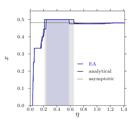
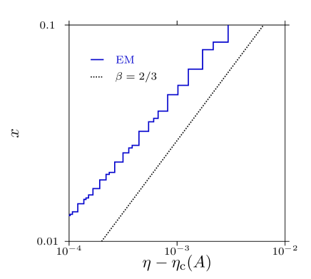
Figure 8: (color online) $x(\eta)$ for $A=0.93$. Left panel: occupation index $x$ vs dimensionless distance $\eta$. We identify successively structures I, $\textrm{I}_{x}$, H, $\textrm{I\kern-1.29167ptI}_{x}$, $\textrm{P}_{1}$, II, III, a range of unclassified phases, and finally structures $\textrm{V}_{x}$ (see also Fig. 4). EA results (blue) and analytical results (black) are shown. In the region of stability of structure $\textrm{I}_{x}$ (i.e., for $x\leq 1/3$), the discrete $x$-values as predicted by the analytic approach (and assuming an idealized version of phase I_x – see related $x$-values specified in Eq. (23)) characterize the staircase-like form of the curve. The regions of constant $x$ are very thin for this value of $A$, close to unity. In addition, $x$-values that are not compatible with Eq. (23) could be identified within the EA approach. Shaded areas indicate overcharging, i.e., where $x>x^{*}$, see Eq. (6). The value of $x^{*}$ is indicated by a dashed line; see the discussion in Subsec. VI.1 for overcharging. Right panel: double-logarithmic plot of $x$ versus $(\eta-\eta_{\rm c})$, as obtained in the EM calculations. The dotted black line is a guide to the eye, indicating the critical exponent $\beta=2/3$, see Eq. (35).

A more thorough discussion of critical features is available in Appendix D. We recall that the above analytical treatment is rigorous only in the asymptotic limit $A\to 1$ (i.e., when $\eta_{c}\to 0$), due to absence of local deformations of the structures on the plates. For other values of the asymmetry parameter $A$, the values of the critical indices have to be checked numerically along the whole critical line, separating phases I and $\textrm{I}_{x}$. An example is given in Fig. 8: for $A=0.93$, the left panel of this figure shows the $x(\eta)$-curves as calculated analytically and by using the EA approach. One observes that $x$ grows quickly with $\eta$ for $\eta>\eta_{c}$, the curve being characterized by very thin plateaus at the anticipated discrete values – see Eq. (23). According to Eq. (35), the analytical approach predicts that the transition $\textrm{I}\to\textrm{I}_{x}$ is of second-order with a critical exponent $\beta=2/3$ for the order parameter $x$ along the whole critical line $\eta_{c}=\eta_{c}(A)$ that separates phases I and I_x. Our numerical EA and EM data corroborate this prediction. For the particular value of $A=0.93$, the plot of $x$ vs. $\eta$ close to $\eta_{c}$ is presented in a double-logarithmic representation in the right panel of Fig. 8. Although even small inaccuracies in the determination of $\eta_{\rm c}$ can severely change the slope of this curve, the shape of $x(\eta)$ does seem compatible with the analytical prediction (the dotted black line). Analogous results were obtained for other values of $A$ when the transition $\textrm{I}\to\textrm{I}_{x}$ takes place.

IV.4 Phase $\textrm{I\kern-1.29167ptI}_{x}$

In phase II, with its structure shown in the right panel of Fig. 2, parallel rows of blue (to be indexed ‘b’) and red (to be indexed ‘r’) particles appear in an alternating sequence on plates 1 and 2, respectively, connected in Fig. 7 by dotted horizontal lines. We can formally assign to this particular periodic repetition of rows the symbol [br], thus $x=1/2$.

The entire family of II_x structures can be constructed by combining the two building elements [br] and [bbr]; phases II_x can be characterized by $x$-values in the range $x\in[1/3,1/2]$. Examples for structures II_x are given in Fig. 7: (i) the previously discussed phase H (being an intermediate structure between phases I_x and II_x) is specified by the sequence of rows [bbr] and $x=1/3$, thus II_x=1/3 = H (see central panel of Fig. 7). Phase $\textrm{I\kern-1.29167ptI}_{x}$ with $x=2/5$, shown in the right panel of Fig. 7, is formally represented by the periodically repeated sequence [br][bbr]. From a more global perspective, the family of structures $\textrm{I\kern-1.29167ptI}_{x}$ represents the transition phase from structure H to structure II and eventually to phase III.

From an alternative point of view, the lattices on layer 2 of the family of structures II_x can be viewed as a sequence of (slightly distorted) triangular and rectangular rows. Lines that connect particles of layer 1 (2), respectively, (as shown as an example in the right panel of Fig. 7), can generate rows of triangles and rectangles via the following simple rules: (i) a blue line followed by a red line produces a row of rectangles, while (ii) two blue lines followed by a red line lead to a row of equilateral triangles. With these two building entities at hand, $x$ can be varied continuously between the values $1/3$ and $1/2$, i.e., a range of $x$-values characteristic for the structures II_x. It should be emphasized that this decomposition into rectangles and triangles represents an idealized view of structures II_x as they are identified via the numerical tools. These combinations of structural units lead in layer 1 to rings which can be quite elongated or can have more complicated shapes, while the lattice in layer 2 consists of slightly distorted rectangles and triangles. We note that similar, alternating sequences of triangles and rectangles have been identified in colloidal structures as precursors of quasi-crystalline structures mikhael_2008 .

Within the analytic approach the series representations of the energies of the phases $\textrm{I\kern-1.29167ptI}_{x}$ can be derived in an analogous way as for phase II, using, however, a more general application of the Poisson summation formula (9). As an example, we outline in the following how to obtain the series representation of the energy of phase H (corresponding to a [bbr] sequence of rows) with $x=1/3$. Denoting by $\Delta$ and $a\Delta$ the lattice spacings of the rectangular structure, we have

$$a^{2}\Delta=\frac{2}{\sigma_{1}+\sigma_{2}}=\frac{2}{n_{1}+n_{2}}.$$ (38)

The total energy per particle of this phase can be written as

$$\frac{E_{\textrm{I\kern-0.90417ptI}_{x}}(\eta;x=1/3)}{Ne^{2}\sqrt{\sigma_{1}+\sigma_{2}}}=2^{3/2}\pi\eta\left(\frac{1}{3}-\frac{A}{1+A}\right)^{2}+\frac{1}{3}\frac{\sqrt{\Delta}}{2^{3/2}}\left(2E_{\rm b}+E_{\rm r}\right),$$ (39)

where

$$E_{\rm b} = \sum_{j,k\atop(j,k)\neq(0,0)}\frac{1}{\sqrt{(3j)^{2}+\Delta^{2}k^{2}}}+\sum_{j,k}\frac{1}{\sqrt{(3j+1/2)^{2}+\Delta^{2}(k+1/2)^{2}}}$$ (40)

$$+\sum_{j,k}\frac{1}{\sqrt{(3j+1)^{2}+\Delta^{2}k^{2}+(d/a)^{2}}}+\sum_{j,k}\frac{1}{\sqrt{(3j+3/2)^{2}+\Delta^{2}(k+1/2)^{2}}}$$

$$+\sum_{j,k}\frac{1}{\sqrt{(3j+2)^{2}+\Delta^{2}k^{2}}}+\sum_{j,k}\frac{1}{\sqrt{(3j+5/2)^{2}+\Delta^{2}(k+1/2)^{2}+(d/a)^{2}}}$$

$$-\mbox{backgr.}$$

is the (dimensionless) energy counted from the point of view of blue (index ’b’) particles on plate 1 and

$$E_{\rm r} = \sum_{j,k\atop(j,k)\neq(0,0)}\frac{1}{\sqrt{(3j)^{2}+\Delta^{2}k^{2}}}+\sum_{j,k}\frac{1}{\sqrt{(3j+1/2)^{2}+\Delta^{2}(k+1/2)^{2}+(d/a)^{2}}}$$ (41)

$$+\sum_{j,k}\frac{1}{\sqrt{(3j+1)^{2}+\Delta^{2}k^{2}+(d/a)^{2}}}+\sum_{j,k}\frac{1}{\sqrt{(3j+3/2)^{2}+\Delta^{2}(k+1/2)^{2}}}$$

$$+\sum_{j,k}\frac{1}{\sqrt{(3j+2)^{2}+\Delta^{2}k^{2}+(d/a)^{2}}}+\sum_{j,k}\frac{1}{\sqrt{(3j+5/2)^{2}+\Delta^{2}(k+1/2)^{2}+(d/a)^{2}}}$$

$$-\mbox{backgr.}$$

is the energy with respect to red (index ’r’) particles on plate 2. After a series of transformations akin to those presented in Refs. Samaj12_1 ; Samaj12_2 , the total energy is expressible in terms of the $K$-function (81) and the function $c(\Delta)$, specified in Eq. (18), as follows

$$\frac{E_{\textrm{I\kern-0.90417ptI}_{x}}(\eta;x=1/3)}{N}=2^{3/2}\pi\eta\left(\frac{1}{3}-\frac{A}{1+A}\right)^{2}+c(\Delta)+\frac{1}{3\sqrt{2}}\left[-K(\Delta,\eta)+\frac{1}{\sqrt{3}}K(3/\Delta,\eta/\sqrt{3})\right].$$ (42)

For the $\Delta$-value of the hexagonal phase, i.e., $\Delta=\sqrt{3}$, phase $\textrm{I\kern-1.29167ptI}_{x=1/3}$ becomes identical to phase H pictured in the central panel of Fig. 7: actually, assuming $\Delta=\sqrt{3}$ in Eq. (42) and recalling that the Madelung constant of the hexagonal lattice is given by $c=c(\sqrt{3})$, one indeed recovers the energy $E_{\textrm{I}_{x=1/3}}$ specified in Eq. (27), i.e., the energy of the phase H; these considerations provide a check for the internal consistency of the formalism.

Since the projected positions of the particles of both layers form an almost perfect hexagonal lattice both in phases $\textrm{I}_{x}$ and $\textrm{I\kern-1.29167ptI}_{x}$, these structures can be characterized by the criterion $0.9<\Psi_{6}^{(3)}$ (see Table 1). Structures $\textrm{I}_{x}$ and $\textrm{I\kern-1.29167ptI}_{x}$ are complementary from the point of view of the occupation parameter $x$ which is constrained to $0<x<1/3$ for phases $\textrm{I}_{x}$ and to $1/3<x<1/2$ for phases $\textrm{I\kern-1.29167ptI}_{x}$. Finally, due to the complexity of the emerging structures within the family of phases the $\textrm{I\kern-1.29167ptI}_{x}$, the last phase that could be taken into account within the analytical treatment corresponds to the sequence [br][bbr][bbr]; it is characterized by $x=3/8$.

V Structures emerging for large $\eta$: $\textrm{V}_{x}$

If the asymmetry parameter $A$ is small, the prefactor in Eq. (20) is large and the transition from phase I to another competitive phase occurs at larger $\eta_{c}$; to be more specific, this particular scenario occurs for $A\lesssim 0.408$, or equivalently for $\eta\gtrsim 0.450$. At large distances between the plates, a particle moving from plate 1 to plate 2 can “loose” the information about its Wigner monolayer position in phase I and can create, together with all the other displaced particles, a completely new, energetically favorable structure. Since local deformations of the sublattices $\alpha$ and $\beta$ are now substantial for large $\eta_{c}$ the analytical approach is no longer trustworthy, as it cannot grasp the distortions; this refers especially to the identification of the order of phase transition which should rather be investigated by numerical tools.

V.1 Phase $\textrm{V}_{x}$

Starting again off from the monolayer structure I, an alternative strategy to populate layer 2 is realized below $A\simeq 0.408$. The emerging family of structures is termed $\textrm{V}_{x}$, as it maintains many of the characteristic features of structure V which is the lowest-energy phase for symmetrically charged plates at sufficiently large distances $\eta$ (see Subsection II.2). We mention that one way to describe the emergence of this structure was discussed in Ref. Ant14 via the so-called “in-branch”, i.e., by approaching one single charge from infinite distance to a perfectly ordered hexagonal monolayer of charges.

In its idealized version (amenable to the analytical treatment), phase $\textrm{V}_{x}$ consists of two hexagonal structures, sublattice $\alpha$ (spacing $a$) at plate 1 with $N_{1}=(1-x)N$ particles and sublattice $\beta$ (spacing $b$) at plate 2 with $N_{2}=xN$ particles; the sublattices are shifted with respect to one another in such a way that all particles of $\beta$, when projected to plate 1, are located in the center of some of the triangles of sublattice $\alpha$. The spacings of the sublattices are related by the equality

$$\frac{S}{N}=\frac{\sqrt{3}}{2}a^{2}(1-x)=\frac{\sqrt{3}}{2}b^{2}x.$$ (43)

Similarly to the case of phase $\textrm{I}_{x}$, joining arbitrary two vertices of sublattice $\alpha$ implies a “commensurate” spacing of sublattice $\beta$, so the sublattice spacings $a$ and $b$ are constrained by

$$\frac{a^{2}}{b^{2}}=\frac{1}{j^{2}+jk+k^{2}}=\frac{n_{2}}{n_{1}}.$$ (44)

Now all possible integer values are allowed for $(j,k)$, except for $(0,0)$; thus we obtain

$$x=\frac{n_{2}}{n_{1}+n_{2}}=\frac{1}{1+j^{2}+jk+k^{2}},\qquad x\in\left\{\frac{1}{2},\frac{1}{4},\frac{1}{5},\frac{1}{8},\frac{1}{10}\ldots\right\}.$$ (45)

In general, both commensurate and incommensurate versions of structure $\textrm{V}_{x}$ exist, as can be seen from the examples given in Fig. 9. As the two substructures $\alpha$ and $\beta$ are characterized by two (perfect or non-ideal) hexagonal lattices located at each of the plates, we can identify phase V_x via the BOOPs $0.9<(1-x)\Psi_{6}^{(1)}+x\Psi_{6}^{(2)}$ (see also Table 1).

The panels of Fig. 9 show representative snapshots of structure $\textrm{V}_{x}$ for three selected state points. These panels confirm that in many – but not all – realizations of this phase, particles in layer 2 are positioned above the centers of triangles in layer 1; further, slight distortions are commonly encountered for intermediate values of $\eta$. For large $\eta$-values the two layers form essentially uncorrelated hexagonal lattices.

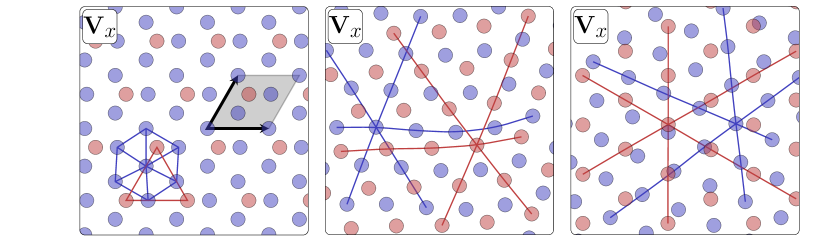
Figure 9: (color online) Representative snapshots of structure $\textrm{V}_{x}$ (see text), with same graphical convention as in Fig. 7. structural features in layers 1 and 2,respectively. Left panel: structure $\textrm{V}_{x}$ for $\eta=0.707$ and $A=0.5$, with $x=1/4$; this $x$-value allows for perfect commensurability of the two sublattices. Center panel: structure $\textrm{V}_{x}$ for $\eta=0.7$ and $A=0.9$, with $x=13/28\simeq 0.464$. Note the wave-like modulation of the hexagonal sublattices (as emphasized by the red and the blue lines). Right panel: structure $\textrm{V}_{x}$ for $\eta=1.061$ and $A=0.7$, with $x=12/31\simeq 0.387$. For large values of $\eta$, there is essentially no correlation between the two layers, leading to a Moiré-type pattern moire .

Within the idealized assumption of the analytic approach, each particle of sublattice $\beta$, when projected onto plate 1, is located in the center of a triangle of sublattice $\alpha$ and therefore sees the same relative array of lattice-$\alpha$ sites, i.e., particles of $\beta$ have topologically equivalent positions. Note that this is no longer true for $\alpha$-particles which group into more topologically non-equivalent sets. When calculating the interaction energy between particles on sublattice $\alpha$ and particles on sublattice $\beta$, it is advantageous to evaluate the full interaction energy of one $\beta$-particle with all $\alpha$-particles and then simply multiply the result by $N_{2}$. Using the summation techniques developed in Ref. Samaj12_2 and the formula (72), we obtain the energy of phase $\textrm{V}_{x}$ in the form

$$\frac{E_{\textrm{V}_{x}}(\eta,A;x)}{Ne^{2}\sqrt{\sigma_{1}+\sigma_{2}}}=2^{3/2}\pi\eta\left(x-\frac{A}{1+A}\right)^{2}+c\left[(1-x)^{3/2}+x^{3/2}\right]+J(x,\eta),$$ (46)

where

$$J(x,\eta) = x\sqrt{1-x}\frac{1}{2^{3/2}\sqrt{\pi}}\int_{0}^{\infty}\frac{{\rm d}t}{\sqrt{t}}\left[-{\rm e}^{-t\eta^{2}(1-x)}+\sqrt{3}{\rm e}^{-3t\eta^{2}(1-x)}\right]$$ (47)

$$\times\left\{\left[\theta_{3}({\rm e}^{-\sqrt{3}t})\theta_{3}({\rm e}^{-t/\sqrt{3}})-1-\frac{\pi}{t}\right]+\left[\theta_{2}({\rm e}^{-\sqrt{3}t})\theta_{2}({\rm e}^{-t/\sqrt{3}})-\frac{\pi}{t}\right]\right\}.$$

The first term on the rhs of Eq. (46) is the excess energy due to the non-neutrality of each of the plates, the second term corresponds to the neutralized intra-layer sums of hexagonal structures within plate 1 and within plate 2; finally, the integral $J(x,\eta)$ describes the interlayer interaction between electro-neutral plates 1 and 2. For the special case $x=0$, Eq. (46) in combination with relation (47), reduces to the energy of phase I, specified in Eq. (19). The series representation of the energy difference $[E_{\textrm{V}_{x}}(\eta,A;x)-E_{\textrm{I}}(\eta,A)]$, suitable for numerical calculations, is presented in Eq. (86) of Appendix C.

Strictly speaking, the energy formula (46) was derived for an idealized phase $\textrm{V}_{x}$ with commensurate discrete values of $x$ given by Eq. (45). However, we ignore henceforward the discreteness of $x$ and apply the formula given in Eq. (46) also to continuous values of $x$.

V.2 Transition I $\to$ V_x

The analytical approach, based on the comparison of the energies (19) and (46) of the competing phases I and V_x, predicts a transition line I $\to$ $\textrm{V}_{x}$ which is in a very good agreement with the EA estimate, as shown in Fig. 4. However, within the analytic approach, the phase transitions are found to be discontinuous (i.e., of first order), accompanied by a discontinuous change of $x$ from 0 to a small, non-vanishing value at the transition point; this scenario differs from the previously discussed second-order transitions between phases I and $\textrm{I}_{x}$. In contrast, our numerical results (based on the EA) provide evidence that the transition between phases I and $\textrm{V}_{x}$ is continuous as well, with constant values of critical exponents along the whole critical line $\eta_{c}(A)$. These values coincide with those obtained for the transition I $\to$ $\textrm{I}_{x}$ (see Subsection IV.3). Hence we conclude that the neglect of local lattice distortions within the analytical treatment is a non-adequate simplification of the problem.

For the special value $A=0.38$, the left panel of Fig. 10 shows the analytical and EA estimates of the curves $x(\eta)$, along which we identify only structures I and $\textrm{V}_{x}$. While we know that some preferred, discrete values of $x$ exist for structure $\textrm{V}_{x}$ [see Eq. (45)], the $x(\eta)$-curve turns out to be basically continuous and smooth. This is due to the fact that at these transitions $\eta$ assumes rather large values, leading to a relatively weak effective interaction between the two layers such that the commensurability of the lattice spacings is no longer crucial. Interestingly, for this value of $A$, $x(\eta)$ appears to converge only very slowly towards the asymptotic value $x^{*}$ – see Eq. (6). As mentioned before, deformations in the sublattices are rather pronounced which manifests itself in the visible difference in $\eta_{\rm c}$ between the analytic and the numerical approaches. The right panel of Fig. 10 emphasizes the bahaviour close to $\eta_{\rm c}(A)$. A critical exponent $\beta=2/3$ ensues, as for the transition I $\to$ $\textrm{I}_{x}$, addressed in Fig. 8.

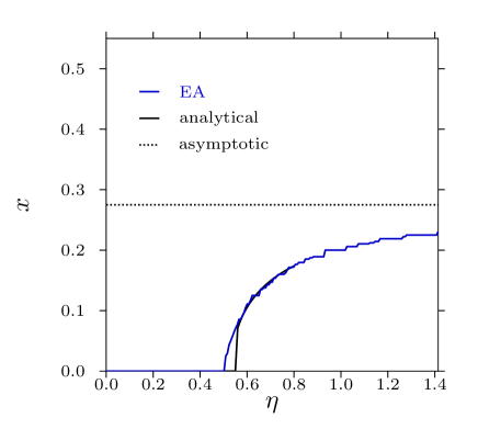
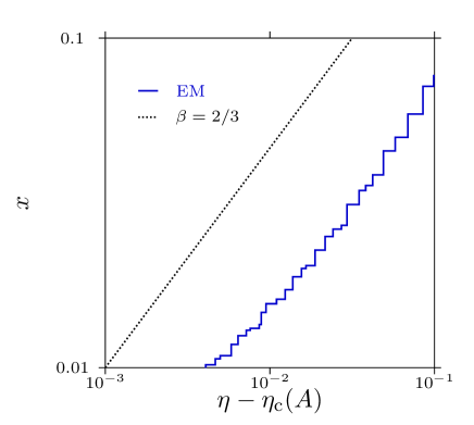
Figure 10: (color online) Plot of $x(\eta)$ for $A=0.38$. Left panel: $x(\eta)$; we identify structures I $(x=0)$ and $\textrm{V}_{x}$ $(x>0)$. EA results are in blue, analytical results in black. As $\eta_{c}$ is rather large, the two layers are correlated only weakly, leading to a smooth curve $x(\eta)$. The asymptotic value $x^{*}$ (see Eq. (6)) is indicated by a dotted line. Note the visible difference in $\eta_{\rm c}$ between the two approaches; this difference is due to deformations in the two sublattices, which are rather pronounced in structure $\textrm{V}_{x}$ close to the bi-critical point (see also panels of Fig. 4). Right panel: double-logarithmic plot of $x$ versus $(\eta-\eta_{\rm c}(A))$. The dotted black line is a guide to the eye, indicating a critical exponent $\beta=2/3$.

In Fig. 4, we show the regions where the monolayer structure I competes with the bilayer structures $\textrm{I}_{x}$ and $\textrm{V}_{x}$. The bi-critical point (with index ’bi’), where these three stability regions meet, was calculated within the EM approach, with the result $\eta_{\rm bi}\simeq 0.470$, $A_{\rm bi}\simeq 0.4085$, and within the EA approach (using smaller cell sizes than in the EM approach, i.e, up to $N=40$ particles per cell), leading to $\eta_{\rm bi}\simeq 0.477$, $A_{\rm bi}\simeq 0.4075$; this point is shown in the panels of Fig. 4 by the white circled asterisk. Close to the bi-critical point, deformations in structures $\textrm{I}_{x}$ and $\textrm{V}_{x}$ are most pronounced: (i) compared to the $\eta$-values where structure $\textrm{I}_{x}$ is stable, $\eta_{\rm bi}$ represents now a rather large value, causing the holes that are left by those particles that moved to layer 2 to contract significantly; (ii) in contrast, for $\eta$-values where structure V_x is stable, $\eta_{\rm bi}$ can be considered to be small and the triangles in layer 1 surrounding particles in layer 2 are distorted significantly. Since in either of the two cases the respective distortions are neglected within the analytical approach, the boundaries separating structure I and structures $\textrm{I}_{x}$ and $\textrm{V}_{x}$ (as predicted by the numerical approach), respectively, differ noticeably in the neighborhood of the bi-critical point (see panels of Fig. 4). In contrast, agreement of the analytical and numerical approaches is found to be excellent both for small and large $\eta$-values, where lattice distortions are small.

V.3 Large-distance behavior of phase $\textrm{V}_{x}$

Numerical approaches have serious convergence problems when dealing with two plates that are separated by large distances due to the fact that the effective interaction energy of the plates is small. On the other hand, an analytical treatment of the large-distance characteristics of phase $\textrm{V}_{x}$ is relatively simple; in fact it becomes exact at asymptotically large values of $\eta$.

A saddle-point calculation presented in Appendix E shows that the integral $J(x,\eta)$ (47), which describes the interaction energy between plates 1 and 2 (each of them begin neutral as a whole) in Eq. (46), behaves at large $\eta$ as follows

$$J(x,\eta)\mathop{\sim}_{\eta\to\infty}-\frac{3^{5/4}}{\sqrt{2}}x\sqrt{1-x}\exp\left(-\frac{4\pi\sqrt{1-x}}{3^{1/4}}\eta\right).$$ (48)

In the symmetric case $x=1/2$, this result has already been obtained in Ref. Samaj12_2 . We emphasize that the exponential decay of the interaction between two plates is not related to the hexagonal structures on the plates, but holds more generally for any pair of plates, each of which is as a whole electro-neutral. We can therefore neglect in the large-$\eta$ limit the inter-layer integral $J(x,\eta)$ in Eq. (46) and consider only intra-layer interactions (from which algebraic decay ensues, as will become clear below):

$$\frac{E_{\textrm{V}_{x}}(\eta;x)}{Ne^{2}\sqrt{\sigma_{1}+\sigma_{2}}}\simeq 2^{3/2}\pi\eta\left(x-\frac{A}{1+A}\right)^{2}+c\left[(1-x)^{3/2}+x^{3/2}\right]\qquad\mbox{for~{}large $\eta$.}$$ (49)

One recognizes in this expression the same structure as invoked in Ref. Messina01 . In the case of interest here, each plate is as a whole not neutral ($x\neq x^{*}$). In the following we derive the optimal occupation index $x$. The energy minimization condition

$$\frac{\partial E_{\textrm{V}_{x}}(\eta;x)}{\partial x}=0=2^{5/2}\pi\eta\left(x-\frac{A}{1+A}\right)+\frac{3}{2}c\left(\sqrt{x}-\sqrt{1-x}\right)$$ (50)

implies the asymptotic behaviour for $\eta\to\infty$

$$x\mathop{\sim}_{\eta\to\infty}x^{*}-\frac{3(-c)}{2^{7/2}\pi}\frac{1-\sqrt{A}}{\sqrt{1+A}}\frac{1}{\eta}.$$ (51)

This relation proves that, as soon as $A\neq 1$, the plates (each as a whole) remain charged up to infinite distance. Since the Madelung constant $c$ is a negative number, $x$ approaches to its asymptotic “neutral” value $x^{*}$ from below. Note that the case $A=1$ is specific in the sense that we always have $x=1/2$, irrespective of the value of $\eta$. For this case the energy of structure V behaves as

$$\frac{E_{\textrm{V}}(\eta,A)}{Ne^{2}\sqrt{\sigma_{1}+\sigma_{2}}}\mathop{\sim}_{\eta\to\infty}c\left[\left(\frac{1}{1+A}\right)^{3/2}+\left(\frac{A}{1+A}\right)^{3/2}\right]-\frac{9c^{2}}{2^{11/2}\pi}\frac{(1-\sqrt{A})^{2}}{1+A}\frac{1}{\eta}.$$ (52)

Finally one obtains

$$\frac{E_{\textrm{V}}(\eta,A)-E_{\textrm{V}}(\eta\to\infty,A)}{Ne^{2}\sqrt{\sigma_{1}+\sigma_{2}}}\mathop{\sim}_{\eta\to\infty}-\frac{9c^{2}}{2^{11/2}\pi}\frac{(1-\sqrt{A})^{2}}{1+A}\frac{1}{\eta},$$ (53)

i.e., at large distances also the ground state energy approaches its asymptotic value from below and the two plates attract each other. As one can see from Eq. (53), the asymptotic approach of the lhs of Eq. (53) is rather slow (i.e., as $1/\eta$), due to the non-neutrality of the plates, except for the symmetric plates $A=1$ when the prefactor vanishes and one recovers an exponential decay with distance GoPe96 ; Samaj12_1 .

For completeness, we also write the inter-plate pressure following from the energy difference specified in relation (53), now in terms of the unscaled distance $d$:

$$P=-(\sigma_{1}+\sigma_{2})\frac{\partial}{\partial d}\frac{E_{\textrm{V}}}{N}\sim-(\sigma_{1}+\sigma_{2})e^{2}\,\frac{9c^{2}}{2^{5}\pi}\frac{(1-\sqrt{A})^{2}}{1+A}\frac{1}{d^{2}}.$$ (54)

It should be emphasized that this equation holds except for $A=0$: indeed, when plate 2 is neutral ($\sigma_{2}=0$), phase I is stable for any interplate separation $\eta$ (see the discussion of limiting cases discussed in Subsection II.1) and $P=0$. In other words, we face two non-commuting limits:

$$\lim_{d\to\infty}\lim_{A\to 0}\,d^{2}P=0,\qquad\lim_{A\to 0}\lim_{d\to\infty}\,d^{2}P\neq 0.$$ (55)

Further we learn from the panels of Fig. 4 that for special $x$-values the respective structures are able to extend over larger $\eta$-ranges, leading to the characteristic stripe pattern in the $\Psi$RGB color schemes shown in of Fig. 4. There is, however, a representative region in the $(\eta,A)$-plane where a different mechanism appears to be at work: for $A\gtrsim 0.7$, the $\Psi$RGB-color schemes provide evidence of regions where the colors change smoothly. A closer look at the corresponding snapshots reveals a wave-like modulation of the hexagonal sub-lattices in the two layers of the respective V_x structures, allowing for an optimized correlation between the lattices in the two layers without significantly decreasing the hexagonal order of either of the layers or preventing a favorable value of $x$ (see center panel of Figure 9). In contrast, a different mechanism is at work for structures $\textrm{V}_{x}$ for $A\lesssim 0.7$ and large $\eta$-values, where the two sublattices are essentially uncorrelated hexagonal particle arrangements, creating thereby a Moiré-type pattern moire (see right panel of Fig. 9).

VI Structures emerging at intermediate $\eta$: II, III, IV; $\textrm{S}_{\bm{1}}$, $\textrm{S}_{\bm{2}}$; $\textrm{P}_{\bm{1}}$, $\textrm{P}_{\bm{2}}$ and $\textrm{P}_{\bm{3}}$

VI.1 Structures II, III, and IV; overcharging

We now return to the structures II, III, and IV, identified as the ground state structures in the symmetric setup, and investigate their role in the diagram of states as charge asymmetry is introduced. Surprisingly we have found that these structures do display a significant role for $A$-values down to $\sim 0.9$ (see the orange, red, and cyan regions in the panels of Fig. 4).

In the asymmetric case, the analytical results show that the two layers remain charged up to arbitrarily large plate separations $\eta$. In an overwhelming portion of the $(\eta,A)$-plane layer 1 carries more point charges than required to compensate for the neutralizing background, leading therefore to a negative net charge on this layer (corresponding to $x<x^{*}$); consequently layer 2 is “underpopulated” by particles and it carries a positive net charge, the so-called undercharging scenario. Here, at a fixed value $A$, $x(\eta)$ tends monotonically increasing towards the limiting value $x^{*}(A)(<1/2)$ – see Fig. 10.

However, since the three symmetric structures II, III and IV are characterized by $x=1/2>x^{*}(A)$, their appearance for $A\gtrsim 0.9$ implies that now layer 2 has to carry a negative net charge, the so-called overcharging scenario. As can be seen in Fig. 8, $x(\eta)$ is now for a fixed value of $A$ a non-monotonous function, which exceeds in the $\eta$-range where the overcharging scenario takes place the threshold value $x^{*}(A)$ and then tends towards this limiting value “from below”.

For the symmetric case (i.e., $A=1$), a rigorous analysis of second-order transitions II $\to$ III and III $\to$ IV has been presented Refs. Samaj12_1 ; Samaj12_2 . These transitions belong to the Landau family with the mean-field value of the critical index $\beta=1/2$. The analysis can be readily extended to the asymmetric case (i.e., $A<1$) and leads to the same result, namely $\beta=1/2$. Consequently and rather noteworthy, fixing the asymmetry parameter $A$ at an arbitrary value within the interval $[0.9,1]$ and changing continuously the distance $\eta$ from 0 to $\infty$, at least two different kinds of second-order phase transitions take place: the first one (I $\to$ $\textrm{I}_{x}$) is characterized by the non-classical critical index $\beta=2/3$, while the other ones (i.e., II $\to$ III and III $\to$ IV) are of mean-field type with $\beta=1/2$.

VI.2 Snub square structures $\textrm{S}_{1}$ and $\textrm{S}_{2}$

In addition to the honeycomb phase H (see Sec. IV), we have identified within the EA approach two further structures that are characterized by $x=1/3$; these phases occupy a substantial region for intermediate $\eta$-values in Fig. 4. Due to the specific features of their lattices that are reminiscent of the ideal snub square lattice (see, for instance, Ant11 and references therein), we denote them as snub square structures, $\textrm{S}_{1}$ and $\textrm{S}_{2}$. Representative snapshots are shown in two panels of Figure 11. Structure $\textrm{S}_{1}$ is essentially amenable to an analytical calculation, unlike $\textrm{S}_{2}$ that is too complex. The two structures are characterized by the following geometric features:

• Structure $\textrm{S}_{1}$ consists of a slightly distorted snub square particle arrangement in layer 1, built up by squares and equilateral triangles. Particles in layer 2 are positioned above the centers of the squares in layer 1, thus forming a square lattice (see right panel of Fig. 11). This structure can be characterized by $x=1/3$, $0.9<\Psi_{5}^{(1)}$ and $0.9<\Psi_{4}^{(2)}$;

• Structure $\textrm{S}_{2}$ consists of a strongly distorted snub square particle arrangement in layer 2 and pentagonal structural units in layer 1 (see center panel of Fig. 11). The structure can be characterized by $x=1/3$ and $0.45<\Psi_{5}^{(2)}$.

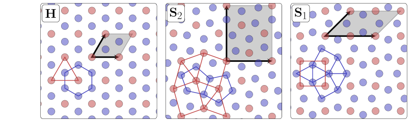
Figure 11: (color online) Representative snapshots of structures H, $\textrm{S}_{2}$, and $\textrm{S}_{1}$ (see text), with the same graphical conventions as earlier. Left panel: structure H for $\eta=0.198$ and $A=0.85$. Center panel: structure $\textrm{S}_{2}$ for $\eta=0.417$ and $A=0.7$. Right panel: structure $\textrm{S}_{1}$ for $\eta=0.622$ and $A=0.675$. In all cases $x=1/3$.

The reason why snub square lattices lead to significant values of the five-fold BOOPs $\Psi_{5}^{(1)}$ and $\Psi_{5}^{(2)}$ is related to the angles that are required for the formation of such a lattice (considering, in particular, its idealized version). As in all of the Archimedean tilings Gruenbaum87 ; Ant11 , each vertex of the snub square tiling (represented by a particle) has exactly the same geometrical surrounding. Since the particular sequence of polygons which characterize the vertices of the (ideal) snub square tiling is specified by [$\triangle-\Box-\triangle-\Box-\triangle$], the required bond angles are given by (see dotted black lines in Fig. 12):

$$\phi_{\rm snub-square}=\left\{\begin{array}[]{l}0,\cr\displaystyle\pm\pi/3,\cr\pm\displaystyle 5\pi/6\simeq\pm 0.833\pi.\end{array}\right.$$ (56)

The values of these angles turn out be very close to the bond-angles of a perfect pentagonal surrounding of the tagged particle (see dotted green lines in Fig. 12), namely

$$\phi_{\rm pentagonal}=\left\{\begin{array}[]{l}0,\cr\pm\displaystyle 2\pi/5,\cr\pm\displaystyle 4\pi/5=\pm 0.800\pi.\end{array}\right.$$ (57)

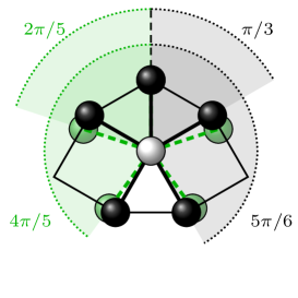
Figure 12: (color online) Schematic view of the immediate neighborhood of a tagged particle (in white) of the ideal snub square tiling, formed by the neighboring black particles. Proceeding clockwise from the top, the vertices are formed by the following sequence of surrounding polygons: $\triangle-\Box-\triangle-\Box-\triangle$. The respective values of the bond angles (indicated by the grey shaded sectors, limited by the dotted black lines) are close to the ones of a perfect pentagonal arrangement (indicated by the green particles, the green shaded sectors, limited by the dotted green lines).

In the analytical approach, structure $\textrm{S}_{1}$ is assumed to have a perfect snub square lattice in layer 1 and a perfect square arrangement in layer 2 (see Fig. 13). Even though the ensuing number of particles per cell (namely $N=6$) is relatively small for the numerical calculations, this value hits the limit for the analytical approach. Here, the snub square phase is constructed by projecting red particles on plate 2 (which there form a square lattice of side $a$) onto plate 1, which is occupied by blue particles. The resulting unit cell of spatial extent $(2a)\times(2a)$ contains for this structure eight blue and four red particles, so that indeed $x=4/(4+8)=1/3$.

The relative positions of particles in layer 1 with respect to the square lattice (defined by particles in layer 2) is quantified via the parameter $\varepsilon$ (see Fig. 13). The value of $\varepsilon$ is fixed by the requirement that the distance between particles 1 and 2 is equal to the distance between particles 1 and 3 (see Fig. 13), i.e.,

$$(a-2\varepsilon)^{2}=\left(\frac{a}{2}+\varepsilon\right)^{2}+\left(\frac{a}{2}-\varepsilon\right)^{2}.$$ (58)

This equation implies that

$$\varepsilon=a\left(1-\frac{\sqrt{3}}{2}\right).$$ (59)

Eventually, the value of square lattice spacing $a$ follows from the electro-neutrality condition:

$$a=\sqrt{\frac{3}{\sigma_{1}+\sigma_{2}}}=\sqrt{\frac{3}{n_{1}+n_{2}}}.$$ (60)

The positions of the particles on plate 2 on the square lattice can be simply enumerated as the multiples of $a$ in terms of integers $j$ and $k$, i.e., $(ja,ka)$. On the other hand, the positions of the particles on plate 1 can be generated from eight basic positions in an elementary cell of spatial extent $(2a)\times(2a)$ (see Fig. 13): (i) $(a/2,\varepsilon)$, (ii) $(a/2,a-\varepsilon)$, (iii) $(a+\varepsilon,a/2)$, (iv) $(2a-\varepsilon,a/2)$, (v) $(\varepsilon,-a/2)$, (vi) $(a-\varepsilon,-a/2)$, (vii) $(3a/2,-\varepsilon)$, and (viii) $(3a/2,-a+\varepsilon)$; all other positions of particles in layer 1 are obtained by shifting these positions in both spatial directions, i.e., by adding $(2aj,2ak)$ with $j$ and $k$ being integers.

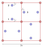
Figure 13: Schematic view of an extended cell for the individual sublayers of spatial extent $(2a\times 2a)$ for the ideal snub square phase. Particles in layer 1 are colored blue, particles in layer 2 are colored red. For the definition of $\varepsilon$ and the particle labels 1, 2, and 3 see text.

Using translation and reflection symmetries for this particular lattice in the lattice sums, it can be shown that the total energy is given by

$$\frac{E_{\rm S_{1}}(\eta)}{Ne^{2}\sqrt{\sigma_{1}+\sigma_{2}}} = \frac{1}{3^{3/2}}\Bigg{\{}\sum_{j,k\atop(j,k)\neq(0,0)}\frac{1}{\sqrt{j^{2}+k^{2}}}+\frac{1}{2}\sum_{j,k}\frac{1}{\sqrt{(j+1/2)^{2}+(k+1/2)^{2}}}$$ (61)

$$+\frac{1}{2}\sum_{j,k}\frac{1}{\sqrt{j^{2}+[k+(1+\sqrt{3})/2]^{2}}}+\frac{1}{2}\sum_{j,k}\frac{1}{\sqrt{(j+1/2)^{2}+(k+\sqrt{3}/2)^{2}}}$$

$$+\sum_{j,k}\frac{1}{\sqrt{[j-(\sqrt{3}+1)/4]^{2}+[k+(\sqrt{3}-1)/4]^{2}}}$$

$$+\sum_{j,k}\frac{1}{\sqrt{[j-(\sqrt{3}-1)/4]^{2}+[k+(\sqrt{3}+1)/4]^{2}}}$$

$$+\sum_{j,k}\frac{1}{\sqrt{(j+1/2)^{2}+(k+\sqrt{3}/2)^{2}+2\eta^{2}/3}}\Bigg{\}}-\mbox{backgr.}$$

Poisson summation formula, Eq. (9) allows to express the lattice summations as quickly convergent series of generalized Misra functions, Eq. (10). For an example of an explicit series representation, we choose the last term in Eq. (61) which is the only term in this relation that depends on the plate distance $\eta$:

$$\sum_{j,k}\frac{1}{\sqrt{(j+1/2)^{2}+(k+\sqrt{3}/2)^{2}+2\eta^{2}/3}}-\mbox{backgr.}\phantom{aaaaaaaaaaaaaaaaaaaaaa}$$ (62)

$$= \frac{1}{\sqrt{\pi}}\int_{0}^{\infty}\frac{{\rm d}t}{\sqrt{t}}{\rm e}^{-2\eta^{2}t/3}\left[\theta_{2}({\rm e}^{-t})\sum_{k}{\rm e}^{-(k+\sqrt{3}/2)^{2}t}-\frac{\pi}{t}\right]$$

$$= \frac{1}{\sqrt{\pi}}\Bigg{\{}2\sum_{j=1}^{\infty}[\cos(\pi\sqrt{3}j)+(-1)^{j}]z_{3/2}[2(\pi\eta)^{2}/3,j^{2}]+4\sum_{j,k=1}^{\infty}(-1)^{j}\cos(\pi\sqrt{3}k)z_{3/2}[2(\pi\eta)^{2}/3,j^{2}+k^{2}]$$

$$+ 2\sum_{j=1}^{\infty}\sum_{k=-\infty}^{\infty}z_{3/2}[0,2\eta^{2}/3+(j-1/2)^{2}+(k+\sqrt{3}/2)^{2}]-\pi z_{1/2}(0,2\eta^{2}/3)\Bigg{\}}.$$

In doing so, the energy of the (ideal) snub square phase can be calculated within the analytic approach rather easily and in an efficient manner.

The situation is considerably more complicated for structure $\textrm{S}_{2}$: here a simplified, yet faithful approximation of this structure requires $N=12$ particles per unit cell, making thus in practice an analytical treatment of this particular phase is currently out of reach.

VI.3 Pentagonal structures $\textrm{P}_{1}$, $\textrm{P}_{2}$ and $\textrm{P}_{3}$

The ordered structures that populate those regions of the $(\eta,A)$-plane that have not been discussed so far are characterized by complicated geometries and symmetry features which prevent them from being amenable to the analytical framework. As $\eta$ and $A$ are varied, these structures change their structural features continuously, rendering a classification of distinct structures difficult. Here we could rely on the support provided by the combined analysis of different sets of BOOPs.

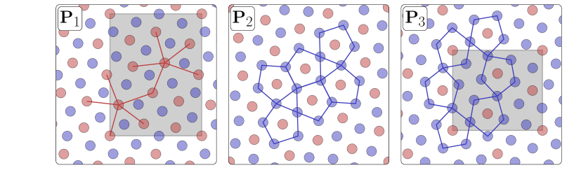
Figure 14: (color online) Representative snapshots of structures with pentagonal features, labeled as structures $\textrm{P}_{1}$, $\textrm{P}_{2}$, and $\textrm{P}_{3}$ (see text). They appear as contiguously colored regions in the $\Psi$RGB-phase diagrams (see panels of Fig. 4). The unit cell is again indicated by the shaded area. Left panel: structure $\textrm{P}_{1}$ for $\eta=0.381$ and $A=0.85$, with $x=12/28\simeq 0.429$. Center panel: structure $\textrm{P}_{2}$ for $\eta=0.346$ and $A=0.825$, with $x=3/8=0.375$. Right panel: structure $\textrm{P}_{3}$ for $\eta=0.410$ and $A=0.6$, with $x=4/18\simeq 0.222$.

We have put particular focus on structures with pentagonal features due to their potential importance with respect to formation of quasicrystals. In the diagram of states (cf. panels of Fig. 4) we have highlighted three regions of stability of structures that are characterized by a local pentagonal order: in particular, they are characterized by a greenish color in the RGB presentations of $\Psi^{(4)}$, indicating thus the dominance of a local pentagonal order. The corresponding representative snapshots are shown in the panels of Fig. 14: Structures $\textrm{P}_{1}$ and $\textrm{P}_{2}$ appear for $x>1/3$, where they compete with structures III and H. Structure $\textrm{P}_{3}$ is characterized by $x<1/3$ and competes strongly with structure $\textrm{I}_{x}$:

• Structure $\textrm{P}_{1}$ is characterized by a complicated particle arrangement and exhibits a pronounced five-fold symmetry in layer 2 (see left panel of Fig. 14). We can characterize phase $\textrm{P}_{1}$ via $1/3<x<1/2$ and $0.45<\Psi_{5}^{(2)}$.

• The characteristic feature of structure $\textrm{P}_{2}$ is the large number of pentagonal holes in layer 1: particles of layer 2 occupy positions above the centers of the pentagons in layer 1 (see center panel of Fig. 14). These particles of layer 2 form a rather well-defined hexagonal lattice. We can characterize phase $\textrm{P}_{2}$ via $1/3<x<1/2$ and $0.9<\Psi_{5}^{(4)}$.

• In a similar manner, structure $\textrm{P}_{3}$ consists of a large number of pentagonal holes in layer 1, albeit with a much lower density (see right panel of Fig. 14). The EA results imply that the region of stability of structure $\textrm{P}_{3}$ also reaches the bi-critical point (marked by a circled asterisk in the panels of Fig. 4). This might be an indication that structure $\textrm{P}_{3}$ represents a transitory phase between structures $\textrm{I}_{x}$ and $\textrm{V}_{x}$. However, even our very fine resolution in the parameters $\eta$ and $A$ within the EA approach is not of sufficient quality for a closer study of this phenomenon; in addition, the complicated geometry of structure $\textrm{P}_{3}$ precludes a more accurate analytical investigation. We have characterized phase $\textrm{P}_{3}$ via $0<x<1/3$ and $0.45<\Psi_{5}^{(4)}$.

VII Results at finite temperature: Monte Carlo simulations

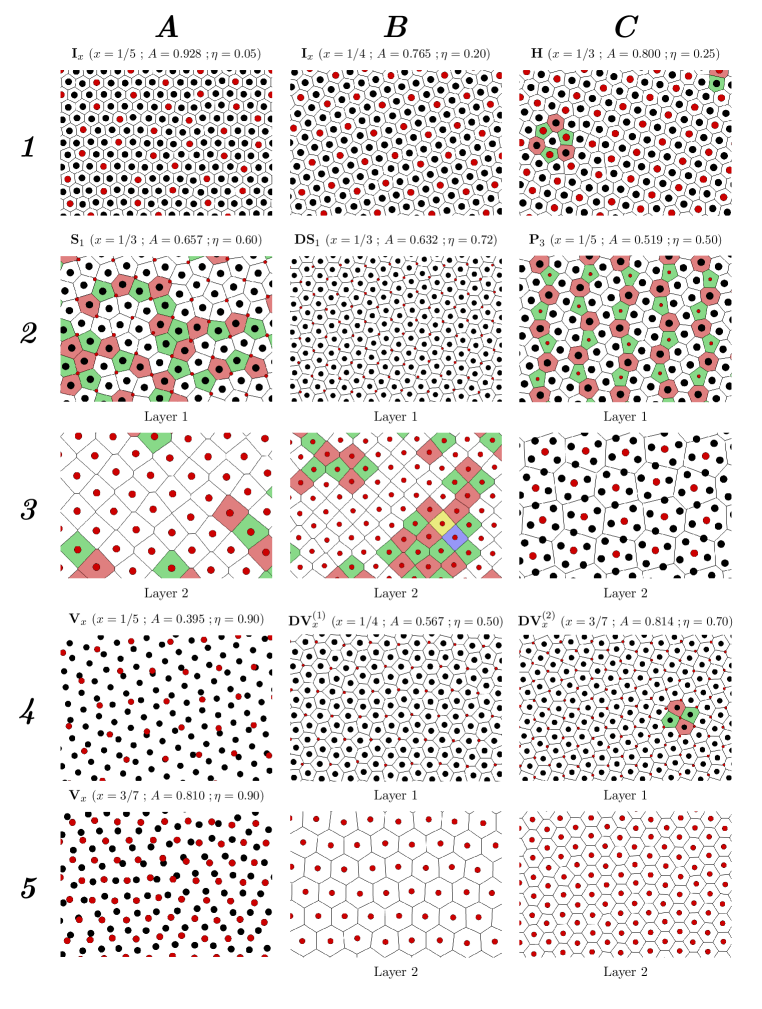
Figure 15: (color online) Snapshots of the principal ordered states obtained in MC simulations along the four domains of constant $x$-values (specified in the text); the respective values of $x$, $A$, and $\eta$ are indicated for each of the snapshots (panels). Particles in layer 1 are indicated in black, while particles in layer 2 are colored in red. For each of the snapshots the respective Voronoi construction is indicated. The color code for the Voronoi cells is the following (color and number of edges): yellow (four), green (five), white (six), red (seven), and blue (eight). For phases I_x and H, the Voronoi constructions have been done with all particles projected onto one plane. Panels are addressed in the text by specifying the column (A to C) and the row (1 to 5).

This section focuses on our comprehensive study of the thermal stability of those ground state configurations that were predicted for vanishing temperature. These investigations, performed via MC simulations at small, but finite temperatures had to be restricted – as a consequence of the high computational costs – to selected state points and relevant regions of the diagram of states. Relevant pathways in the $(\eta,A)$-plane were selected, which are characterized – according to the EA predictions – by constant values of $x$ polynomials . From the seven respective domains highlighted in Fig. 3, we have chosen for the subsequent discussion the ones for $x=$ 3/7, 1/3, 1/4, and 1/5. As can be seen, these pathways cross the regions of stability of several phases. On each of these pathways, the red triangle in Fig. 3 represents the state point which was used as initial configuration, taken from the EA calculation. The subsequent MC runs are then carried out along the lines indicated, for state points located along these pathways (marked by colored symbols). Fig. 15 displays enlarged snapshots of particle configurations as obtained along these pathways; they will be addressed in the following discussions. Additional structures are shown in Appendix F.

The conclusions drawn from our extensive MC simulation are the following:

• structural data extracted agree remarkably well with the corresponding predictions of the EA based investigations; this holds in particular for those state points in the $(\eta,A)$-plane, which are located well within regions of stability of the different structures. This excellent agreement is observed even on a quantitative level, confirmed both by the values of the respective BOOPs as well as by the values of $x$, i.e. the quantity which specifies the particle population on the two planes;

• in the case that these pathways cross limits of stability of competing structures, MC results are able to reflect these competitions faithfully: by a careful structural analysis based on Voronoi constructions, features of the involved competing structures could be identified.

Our MC based observations are detailed in the following, focusing on the above mentioned four domains in the $(\eta,A)$-plane, characterized by a constant $x$-value.

VII.1 The domain $x=3/7$

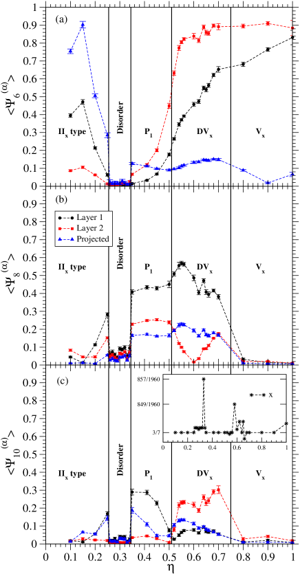
Figure 16: (color online) Bond orientational order parameters computed in MC simulations for runs within the domain $x=3/7$ as functions of the dimensionless distance $\eta$: (a) $\langle\Psi_{6}^{(\alpha)}\rangle$, (b) $\langle\Psi_{8}^{(\alpha)}\rangle$, and (c) $\langle\Psi_{10}^{(\alpha)}\rangle$; results obtained for the different layers ($\alpha$ =1, 2, or 3) are colored according to the labels. In the inset of panel (c), the value of $x=N_{2}/N$ is shown. Occurring ordered (and disordered) structures are labeled.

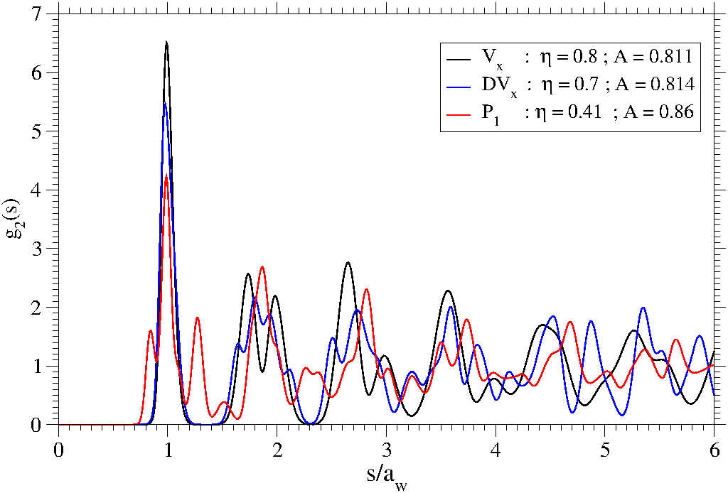
Figure 17: (color online) Center-to-center pair correlation functions as obtained from MC simulations along the domain $x=3/7$. $g_{2}(s)$ for the following three phases: V_x, DV_x, and P₁ (for state points as labeled in the inset). The length used to rescale distances is $a_{\rm w}=(2/\sqrt{3}n_{2})^{1/2}$, $n_{2}$ being the density of the layer.

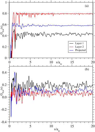
Figure 18: (color online) Bond orientational correlation functions $G_{n,\alpha}(s)$ as defined in Eq. (14) with $n$ and $\alpha$ as labeled as obtained in our simulations along the domain $x=3/7$. (a) $G_{6,\alpha}(s)$ for the DV_x phase ($\eta=0.7$, $A=0.814$) for layer 1, layer 2, and for all particles projected in the same plane (as labeled). (b) $G_{8,\alpha}(s)$ for the P₁ phase ($\eta=0.41$, $A=0.86$) for layer 1, layer 2, and for all particles projected in the same plane (as labeled). The lengths used to rescale distances are $a_{i;{\rm w}}=(2/\sqrt{3}n_{i})^{1/2}$, $n_{i}$ being the density of the respective layer.

The initial configuration for MC simulations in the domain $x=3/7$ is the configuration of the pentagonal phase P₁ as identified in the EA investigations for $\eta=0.410$ and $A=0.86$ (cf. Fig. 3); details of this configuration and the function $A_{x=3/7}(\eta)$, that specifies the asymmetry parameter as a function of $\eta$ in this domain are collected in Table 2 of Appendix F. In Fig. 16, we represent the most significant order parameters; the values of $x=N_{2}/N$, obtained in MC simulations, are shown in the inset of panel (c). The order parameters calculated along the curve $A_{x=3/7}(\eta)$ allow to identify five different phases with decreasing $\eta$: phases V_x, DV_x, and P₁, a disordered phase, and eventually phase II_x.

According to the criteria put forward in Table 1, phases V_x are found for $0.75\lesssim\eta$. An enlarged snapshot of this phase is shown in panel (A5) of Fig. 15; the panel displays a Moiré type pattern composed of equilateral triangles. In the range $0.51\lesssim\eta\lesssim 0.75$, a phase emerges that we denote as the distorted phase V_x (i.e., phase DV_x): in this $\eta$-interval, the six-fold order parameter reaches for both layers still significant values, while $\langle\Psi^{(1)}_{8}\rangle$ for layer 1 and $\langle\Psi^{(2)}_{10}\rangle$ for layer 2 deviate significantly from 0. Further, as can be seen from Fig. 17, the correlation function $g_{2}(s)$ differs (for the state point $\eta=0.7$ and $A=0.814$) distinctively from the correlation functions obtained for the V_x phases (depicted for the state point $\eta=0.80$ and $A=0.811$): the second and third peaks are both split into two secondary peaks, reflecting the distortion of the triangular lattice. In panels (C4) and (C5) of Fig. 15, we represent enlarged snapshots of a typical DV_x structures, along with the related Voronoi constructions for both layers. Further details are provided in Appendix F. The long-range bond orientational function $G_{6,\alpha}(s)$ is shown in panel (a) of Fig. 18. In the subsequent $\eta$-range, i.e., $0.345\lesssim\eta\lesssim 0.51$ the pentagonal phase P₁ is stable, in full agreement with the EA-based analysis. The corresponding correlation function $g_{2}(s)$ is shown in Fig. 17: again we find significant differences with respect to the corresponding correlation functions of the previously discussed phases V_x and DV_x. The long-range bond orientational correlation function $G_{8,\alpha}(s)$ is displayed in panel (b) of Fig. 18.

Within the interval $0.255\lesssim\eta\lesssim 0.345$, no long-range order could be identified at all, as evidenced by the order parameters displayed in Fig. 16; likewise, the intra- and inter-layer correlation functions exhibit no structure (not shown). We encounter here a disordered phase. In this region, EA calculations indicate the close vicinity of the boundaries that separate the regions of stability of several competing phases, namely structures H, II_x, II, II , P₁, and P₂. We interpret the lack of orientational and long-range order observed in the MC simulations at this small temperature as a result of a strong competition between these phases. The abrupt changes in the order parameters close to the boundaries of this $\eta$-regime (i.e., for $\eta\sim 0.345$ and $\eta\sim 0.255$; see Fig. 16) are indications of the coexistence between various phases and of first-order transitions between them. A more quantitative statement on this issue requires significantly larger computational efforts.

Eventually for $\eta\lesssim 0.255$, the Voronoi construction for all particles projected onto the same plane (not displayed) indicates the occurrence of a regular hexagonal tiling with thermal distortions, which we identify as a II_x type phase.

VII.2 The domain $x=1/3$

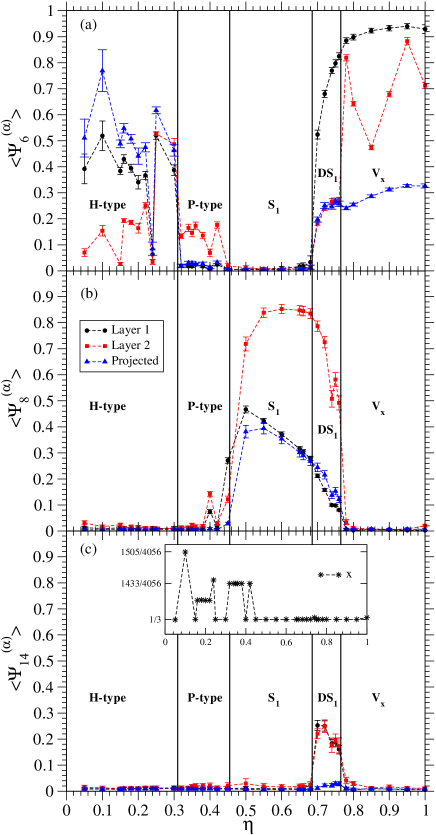
Figure 19: (color online) Same as Fig. 16, for the domain $x=1/3$, and (a) $\langle\Psi_{6}^{(\alpha)}\rangle$, (b) $\langle\Psi_{8}^{(\alpha)}\rangle$, and (c) $\langle\Psi_{14}^{(\alpha)}\rangle$; $\alpha=$1, 2 or 3.

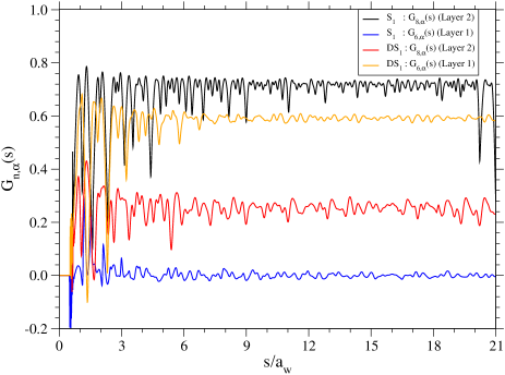
Figure 20: Bond orientational correlation functions $G_{6,\alpha}(s)$ and $G_{8,\alpha}(s)$ (defined in Eq. (14)) as obtained in MC simulations along the domain $x=1/3$ for phases S₁ ($\eta=0.65$ and $A=0.646$) and DS₁ ($\eta=0.74$ and $A=0.629$), as labeled. The lengths used to rescale distances are $a_{i;{\rm w}}=(2/\sqrt{3}n_{i})^{1/2}$, $n_{i}$ being the density of the respective layer.

The initial configuration for MC simulations in the domain $x=1/3$ is the snub square phase S₁ as identified in the EA investigations for $\eta=0.629$ and $A=0.65$ (cf. Fig. 3); details of this configuration and the function $A_{x=1/3}(\eta)$, that specifies the asymmetry parameter as a function of $\eta$ in this domain are collected in Table 2 of Appendix F. We note that within the range $0.31\lesssim\eta\lesssim 0.455$, the curve $A_{x=1/3}(\eta)$ slightly passes through the domain $x=1/3$. In our MC simulations we find in this $\eta$-range $x=1433/4056$ while EA calculations predict $x=6/17$; the two values differ thus by $\sim$ 0.1%.

In Fig. 19, we represent the most significant averaged order parameters for the runs $x=1/3$; the values of $x=N_{2}/N$ are shown in the inset of panel (c). The order parameters calculated allow to identify five different phases with decreasing $\eta$: V_x, DS₁, and S₁, as well as the P-type and the H-type phases. For $0.765\lesssim\eta$, phase V_x is found to be stable. In layer 2 the BOOP $\langle\Psi_{6}^{(2)}\rangle$ is significantly smaller than one, which is due to different orientations of grains in the triangular lattice.

As we decrease the distance between the layers below $\eta\sim 0.765$, structure V_x transforms into a distorted structure with order parameters $\langle\Psi^{(\alpha)}_{6}\rangle$, $\langle\Psi^{(\alpha)}_{10}\rangle$ (not shown), and $\langle\Psi^{(\alpha)}_{14}\rangle$ that differ in their values from those characteristic for phase S₁. For $0.685\lesssim\eta\lesssim 0.765$, layer 2 has a rhombic structure, an enlarged snapshot of this layer along with the respective Voronoi construction is represented in panels (B2) and (B3) of Fig. 15. Particles in layer 1 form a distorted triangular lattice and the Voronoi construction indicates a structure similar to the one formed by isohedrally-tiled hexagons with the symmetry group ${\it p31m}$ (see respective panel in Fig. 15). In this phase, the long-range orientational order, expressed via the bond-orienational correlation functions $G_{6,\alpha}(s)$ and $G_{8,\alpha}(s)$, distinctively differs from the order of structure S₁, as demonstrated by the results shown in Fig. 20. Since the orientational order for layer 2 resembles that of phase S₁, this phase is termed distorted S₁ (i.e., DS₁). The abrupt changes in the order parameters $\langle\Psi^{(\alpha)}_{6}\rangle$ and $\langle\Psi^{(\alpha)}_{8}\rangle$ for $\eta\simeq 0.76$ are indications of a first-order transition between phases DS₁ and V_x; we note that for the symmetric bilayer, a similar mechanism has been identified for the transition between phases IV and V, see Refs. Weis:01 ; Mazars:08 .

The snub square phase S₁ (see panels (A2) and (A3) in Fig. 15) is found to be stable at our chosen finite temperature for $0.455\lesssim\eta\lesssim 0.685$. Further structural details about this phase are shown in Fig. 20 where the bond orientational correlation functions $G_{6,\alpha}(s)$ and $G_{8,\alpha}(s)$ are displayed. The Voronoi construction for particles in layer 1 in the ground state configuration of this phase leads to a so-called Cairo pentagonal tiling Gruenbaum87 with a p4g symmetry. This also holds for layer 2, where we recover a square regular tiling with a p4m symmetry. In Ref. Leipold:15 , the distribution of the number of neighbors for a square lattice under an infinitesimal perturbation of the lattice position was computed; the numerical evaluation of these analytical results yield: $p(4)=p(8)\simeq 0.044$, $p(5)=p(7)\simeq 0.2435$ and $p(6)\simeq 0.4249$. The corresponding values extracted from our MC simulations are in good agreement with these predictions: $p(4)=p(8)\simeq 0.01$, $p(5)=p(7)\simeq 0.22$.

As announced above, in the range $0.31\lesssim\eta\lesssim 0.455$, the $A_{x=1/3}(\eta)$ curve goes through the domain $x=1/3$. The Voronoi construction for all particles projected onto the same plane (not shown) indicates that the majority of the particles in layer 2 have five neighbors in layer 1. These observations fit very well with the definitions of the pentagonal phases (P₁, P₂ and P₃) as found in the EA investigations – see discussion in Subsection VI.3; however, we were not able to identify the phases encountered in the MC simulations with either of the three pentagonal phases, specified via the EA approach.

Eventually, for $\eta\lesssim 0.31$ the EA investigations predict the stability of phase H; within this $\eta$-range MC simulations recover correctly this hexagonal phase, with only a few isolated grains having different orientations. An enlarged snapshot taken from the MC simulations is shown in panel (C1) of Fig. 15: the displayed configuration (obtained for $\eta=0.25$) exhibits the characteristic features of the phase H. As $\eta$ is further decreased along the line $A_{x=1/3}(\eta)$ (and in particular if $\eta\lesssim 0.15$), the hexagonal structures formed by all particles is well preserved while some of the specific features of the sublattices on the individual layers do no longer correspond to the ideal features of phase H, see also Appendix F. It should be emphasized, that for such small $\eta$-values and at finite temperatures, the difference between intralayer and interlayer energies are too small to allow a precise observation of the ideal ground state structure of phase H in MC simulations.

VII.3 The domain $x=1/4$

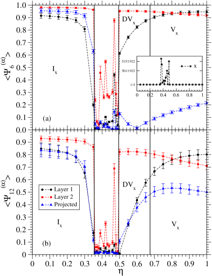
Figure 21: (color online) Same as Fig. 16 for the domain $x=1/4$: (a) $\langle\Psi_{6}^{(\alpha)}\rangle$ and (b) $\langle\Psi_{12}^{(\alpha)}\rangle$.

The initial configuration for MC simulations in the domain $x=1/4$ is the configuration of the phase V_x as identified in the EA investigations for $\eta=1.00$ and $A=0.45$ (cf. Fig. 3); see also Table 2 of Appendix F. Fig. 21 shows the order parameters which allow to identify three different phases with decreasing $\eta$: V_x, DV_x, and eventually phase I_x. Between the two latter ones, there is an $\eta$-range (i.e., for $0.32\lesssim\eta\lesssim 0.49$), where no stable, long-range order could be identified; this observation can be related to the fact that this section of the pathway corresponds to a region along which several ordered structures coexist (cf. Figs. 3 and 4.)

Within the domain $x=1/4$, the phase V_x occurs for $0.67\lesssim\eta$, which is built up by commensurate triangular sublattices in layers 1 and 2; consequently the long-range orientational orders in both layers are particularly stable as the spacing between the layers decreases. The order parameters $\langle\Psi_{6p}^{(\alpha)}\rangle$ ($p$ being a positive integer) reache rather large values (see Fig. 21) and the limiting case embodied in Eq. (15) is well fulfilled. In contrast, all other order parameters $\langle\Psi_{n}^{(\alpha)}\rangle$ with $n\neq 6p$ vanish. As a consequence of the commensurability of the structures on the two sublattices (which can be observed at even large distances between layers, i.e. for $\eta\gtrsim 0.8$), the interlayer correlation function $g_{3}(s)$ exhibits strong correlations for long distances $s$; this fact is in striking contrast to the observations made for other V_x phases (i.e., for other values of $x$).

Decreasing the distance $\eta$, we observe that the hexagonal order in layer 2 is still well preserved for $\eta$-values down to $\simeq 0.5$; in contrast, the hexagonal order in layer 1 is rather strongly distorted for $0.67\lesssim\eta\lesssim 0.7$. The snapshots in panels (B4) and (B5) of Fig. 15 reveal the distortions of the hexagonal cells in layer 1 via the related Voronoi constructions: these distortions have the same vertex topology as the regular hexagonal tiling, but with three different orientations of the distorted hexagons similar to the monohedral convex hexagonal tilings with a p3 symmetry. Because of these continuous distortions of the lattice in layer 1 in this $\eta$-range, we coin this structure again as a distorted V_x phase (DV_x).

For $0.32\lesssim\eta\lesssim 0.49$, no ordered structures with $x=1/4$ could be identified in the EA-based investigations. To gain a better understanding of the transition V_x $\rightarrow$ I_x (which we identify for $\eta\lesssim 0.355$) within the domain $x=1/4$, simulations have been carried out within this particular $\eta$-interval. As shown in the inset of Fig. 21-(a), the extracted values of $x$ deviate in this $\eta$-range significantly from the ideal value of $x=1/4$, an observation similar to the one made in the EA-based investigations. However, no significant stable and long-range order could be identified within the interval $0.32\lesssim\eta\lesssim 0.49$; instead, we have observed some metastabilities of the structure DV_x and some grains of phase I_x=1/4.

For $\eta\lesssim 0.355$ we find – in full agreement with the EA computations (see panel (B1) in Fig. 15 and panel (a) of Fig. 25 in Appendix F), – that phase I_x is stable. As shown in Fig. 25-(a), the Kagomé lattice for particles in layer 1 and the triangular lattice for particles in layer 2 are perfectly recovered.

VII.4 The domain $x=1/5$

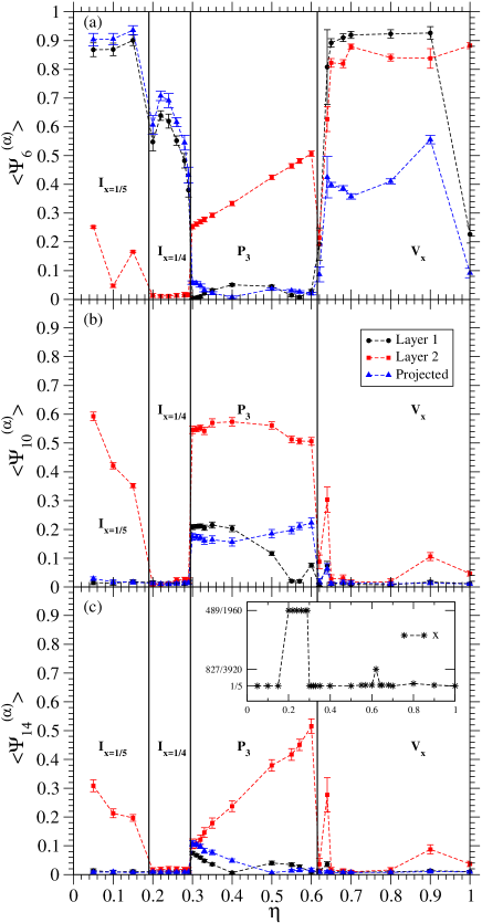
Figure 22: (color online) Same as Fig. 16, for $x=1/5$: (a) $\langle\Psi_{6}^{(\alpha)}\rangle$ , (b) $\langle\Psi_{10}^{(\alpha)}\rangle$, and (c) $\langle\Psi_{14}^{(\alpha)}\rangle$.

Here, the “seed” for MC simulations is the pentagonal phase P₃ as identified with the EA for $\eta=0.410$ and $A=0.86$ (see details in Table 2 of Appendix F. Fig. 22 allows us to identify four different phases with decreasing $\eta$: V_x, P₃, I_x=1/4, and I_x=1/5. Phase V_x is stable for $0.62\lesssim\eta$. For a snapshot, see panel (A4) of Fig. 15 and Fig. 24-(c) in Appendix F. The formation of grains of phase V_x and the abrupt change in the order parameters for $\eta\simeq 0.61$ (see Fig. 22) are strong indications of a first-order phase transition that occurs as we pass from structure V_x to the subsequent structure P₃.

In the interval $0.295\lesssim\eta\lesssim 0.61$, we encounter the pentagonal phase P₃ (identified by the EA investigations) as a stable phase at finite temperatures. Snapshots of this structure along with the related Voronoi constructions for particles in layer 2 and for all particles projected onto the same plane are presented in panels (C2) and (C3) of Fig. 15. Almost all Voronoi cells with five sides (cells represented in green in (C2)) host particles that belong to layer 2; this observation is in agreement with the definitions specified for phase P₃. The Voronoi construction for particles in layer 2 has a vertex configuration $3^{6}$ and a symmetry pg. Rather large values of the order parameter $\langle\Psi_{10}^{(2)}\rangle\simeq 0.55$ for layer 2 (see panel (b) of Fig. 22) stem from the weights $W_{ij}$ (defined in Eq. (12)) and the pentagonal shape of the Voronoi cells.

Proceeding to smaller $\eta$-values ($0.19\lesssim\eta\lesssim 0.295$), we observe that the MC sampling favors the features of commensurability of phase I_x=1/4; this is corroborated via the following facts: (i) as shown in the inset of Fig. 22-(c), we obtain $x=489/1960$, which differs only by 0.2% from 1/4; (ii) in Fig. 25-(b), we present a corresponding snapshot as obtained for $\eta=0.28$ and $A=0.67$. Grains of phase I_x=1/4 are detected (with Kagomé and triangular lattices formed by particles of layers 1 and 2, respectively). This observation, a fingerprint of thermal effects at finite temperature, can be interpreted as a strong competition between the various structures within the family of I_x phases, found as ground states within EA.

Finally, we have identified phase I_x=1/5 for $\eta\lesssim 0.19$ within the domain $x=1/5$; a snapshot of this structure is shown in panel (A1) of Fig. 15. This particular structure represents an impressive example of the large diversity of phases encountered within the family of I_x structures (see Subsection IV.2): its primitive cell hosts 20 particles and particles in layer 2 do not form a hexagonal lattice.

VIII Conclusions

We have investigated in a comprehensive manner the ordered ground state configurations of a system of identical point charges, immersed into the space confined between two parallel plates (labeled 1 and 2) of opposite charge and separated by a dimensionless distance $\eta$. A state point is defined by a value of $\eta\in[0,\infty]$ and of the asymmetry parameter $A$, which is the ratio of the surface charge densities of the plates ($A=\sigma_{2}/\sigma_{1}$); for symmetry reasons $A$ varies in the range $[0,1]$.

Investigations were predominantly carried out at vanishing temperature, using two approaches: (i) an analytical method and (ii) a highly specialized and reliable optimization technique that is based on ideas of evolutionary algorithms (EA). The methods are complementary in the sense that they mutually compensate for their respective deficiencies: (i) the analytic approach provides essentially exact numerical results for the energy of some candidate structures. However, the method is limited – due to the rapidly increasing complexity of the formalism – to ordered structures that are ideal (i.e., they are free from distortions) and that are not too complicated in their internal architecture; (ii) in contrast, the optimization technique is able to treat highly complex and also possibly distorted structures which are by far out of reach for the analytic approach: unit cells with up to 40 particles could be considered; however, the approach is not able to provide a rigorous proof that a particular structure is indeed the ground state configuration for a specific state point. These investigations were completed by comprehensive Monte Carlo (MC) simulations, carried out at small, but finite temperatures; here we have tested the thermal stability of the particle configurations, which were predicted in the preceding investigations as ground state configurations.

The symmetric Wigner bilayer problem (i.e., $A=1$) is meanwhile well documented in literature: five different ground state configurations (labeled I to V) have been identified in previous investigations. Our generalization of the problem to the asymmetric case (i.e., $0\leq A<1$) leads to a plethora of ordered bilayers whose features can be summarized as follows:

• Even for $A<1$, the phase I (i.e., the hexagonal monolayer at plate 1) remains stable up to an $A$-dependent distance $\eta_{c}(A)$, which monotonously increases with decreasing $A$.

• This monolayer phase competes for $\eta\simeq\eta_{c}(A)$ with the newly emerging phases $\textrm{I}_{x}$ and $\textrm{V}_{x}$: both are bilayer structures where a fraction $x$ of particles has been moved from layer 1 to layer 2. Within high numerical accuracy, there is evidence that the transitions I $\to$ I_x and I $\to$ V_x are both of second order; along the respective critical lines, $\eta_{c}(A)$, the critical exponents acquire non-classical values (as, for instance, $\beta=2/3$). The stability regions of the three phases meet at the bi-critical point, located at $(\eta_{\rm bi}\simeq 0.47,A_{\rm bi}\simeq 0.408)$.

• The region of stability of phase V_x dominates for intermediate and large $\eta$-values (i.e., for $0.7\lesssim\eta$) in the diagram of states. In contrast, for small $\eta$-values we find variations of phase I_x, which transform with monotonously increasing $A$ into the highly stable honeycomb structure H (characterized by $x=1/3$); when further increasing $A$, phases II_x, II, and III emerge. In the range of intermediate $\eta$-values (i.e., up to $\eta\simeq 0.7$) we have identified – in addition to the aforementioned phase V_x – a broad variety of complex, sometimes exotic structures, some of which show a pronounced five-fold symmetry: the snub square phase (which is related to the Archimedean tiling) or pentagonal structures. At the moment, it is difficult to provide a decisive answer if they can be considered as precursors of quasi-crystalline lattices. Work along these lines is in progress.

• In large parts of the $(\eta,A)$-plane, the diagram of states is characterized by rather thin, stripe-shaped regions where the occupation parameter $x$ attains rational values (i.e., 1/2, 1/3, etc.). These $x$-values are imposed by commensurability requirements of the emerging sublattices on the two plates, hence the corresponding structures are rather simple (i.e. they have relatively small unit cells) and are characterized by a high degree of stability.

• Eventually, for $0.9\lesssim A$ we could identify regions in the $(\eta,A)$-plane where the ground state configurations of the symmetric case (phases II to V), are found to be stable. The transitions between phases II $\to$ III and III $\to$ IV are continuous with the critical exponents belonging to the mean-field universality class (i.e., $\beta=1/2$, etc.). Thus we conclude that (at least) two second-order phase transitions can be identified in the diagram of states of our system, pertaining to two different universality classes.

The results obtained via the analytic and the numerical approaches agree remarkably well in those $(\eta,A)$-regions where both methods are applicable (i.e., for not too complex and undistorted particle arrangements). Discrepancies in the boundaries of stability regions are observed in the case that the emerging ordered ground state configurations are highly complex (e.g., lattices with a five-fold symmetry) and/or where the structures deviate via distortions from their idealized version.

The plethora of (sometimes highly complex) structures emerging in the asymmetric Wigner bilayer problem is the result of the competition between two driving forces:

• on one side there is the system’s desire for local charge neutrality, separately on each of the two plates (note that global electroneutrality always holds). This principle is dominant either for the archetypical structures I to V, which were identified for the symmetric case (where $x(A=1)=x_{\rm neutr}=1/2$), or for large interplate distances $\eta$ (where the effective interactions between the layers becomes weak, the layers do not “feel’ each other anymore and thus the two sublattices are essentially uncorrelated).

• On the other side there is the attempt of the particles to self-assemble in commensurate sublattices on the two plates, a strategy which is in particular in place for small and intermediate interplate distances $\eta$: here the two layers are strongly correlated. The commensurability requirement imposes discrete, rational values of $x$.

In the transition region, where neither of the two competing forces is dominant (i.e., at intermediate $\eta$-values), the formerly discrete $x$-values become essentially continuous. The competition between preferred discrete values of $x$ and a continuous increase $x(\eta)$ can serve as an explanation for the intricate shape of the boundary separating structures $\textrm{I}_{x}$ and $\textrm{P}_{3}$ (see Fig. 4), which undulates back and forth with decreasing $A$. The emerging structures represent a compromise between the two disparate driving forces. Except for the symmetric case ($A=1$) and the limiting case $\eta\to\infty$, the system is in general not able to realize this compromise between these two requirements. Thus charge-neutrality is in general violated in either of the two following senses: (i) in an overwhelming portion of the $(\eta,A)$-plane the charged particles attached to plate 1 overcompensate for the surface charge, while the other plate is “underpopulated”; this case is termed undercharging; (ii) yet, for $A\gtrsim 0.9$ we could identify regions in the $(\eta,A)$-plane where this trend is inverted and where we observe overcharging; this occurs in particular in regions where the pure phases II to V are stable.

Finally, another consequence of the local violation of charge-neutrality should be mentioned: (i) in the symmetric case ($A=1$) where both plates (along with the attached charged particles) are neutral, the effective interaction between the layers decreases exponentially with distance; (ii) however, as soon as $A<1$ and local charge-neutrality is violated in either sense, we observe a long-range attraction between the plates which decays as $1/\eta^{2}$.

Extensive, complementary Monte Carlo (MC) simulations have been performed at small, but finite temperatures and in selected regions of the $(\eta,A)$-plane where promising features could be expected. Based on several structural observables (such as bond orientational order parameters or different types of correlation functions) the simulations confirm that the ground state configurations (as they were predicted by the analytic and the numerical approaches) remain in general stable even at small, finite temperatures. This statement does not hold for state points that are located close to phase boundaries that separate competing structures: in these regions, the limiting ensemble size (with typically up to 4000 particles) and the limited simulation time prevent us from making more decisive conclusions on the stability of the emerging structures.

The model at hand is a simple, yet striking example that demonstrates that the emergence of highly complex particle arrangements can easily be triggered via changes in solely two parameters (the interplate distance $\eta$ and the charge asymmetry parameter $A$).

Acknowledgments. M.A. and G.K. gratefully acknowledge financial support by the Austrian Science Foundation (FWF) under projects Nos. P23910-N16 and F41 (SFB ViCoM) and by E-CAM, an e-infrastructure center of excellence for software, training and consultancy in simulation and modelling funded by the EU (Proj. No. 676531). L.Š. acknowledges support from grant VEGA 2/0003/18. All authors acknowledge financial support from the projects PHC-Amadeus-2012 and 2015 (project numbers 26996UC and 33618YH), Projekt Amadée (project numbers FR 10/2012 and FR 04/2015), and funding by Investissement d’Avenir LabEx PALM (grant ANR-10-LABX-0039).

Appendix A From non-neutralized to neutralized plates

The ground state energy $E$ is a function of both $\eta$ and $A$. Likewise, the occupation parameter $x$ is a function of both of these variables. We can extend the definition of the ground state energy to $E(\eta,A;x)$ with a priori independent variables $\eta$, $A$ and $x$. In our investigations we retain for a given state point ($\eta$, $A$) only the configuration with the lowest reduced energy per particle $E(\eta,A)/N$ as the ground state, which is given by

$$E(\eta,A)=\min_{x\in[0,1]}E(\eta,A;x).$$ (63)

Let us consider the general situation when each plate as a whole (i.e. including the ions in residence) has a nonzero charge, i.e., $\sigma_{1}\neq n_{1}$ and $\sigma_{2}\neq n_{2}$, under the overall electro-neutrality constraint (4). Is there a relation between the energy of this configuration of charged plates and the energy of neutralized plates with the surface charge densities $\sigma_{1}=n_{1}$ and $\sigma_{2}=n_{2}$? In connecting the two situations, the ionic configurations is fixed, meaning that $n_{1}$ and $n_{2}$ are fixed. Only the surface charges $\sigma_{1}$ and $\sigma_{2}$ are allowed to change, fulfilling electroneutrality. Microscopically, the total energy of the system (i.e., plates and charges) is given by

$$E(\eta,A;x)=E_{pp}+E_{ps}+E_{ss},$$ (64)

where $E_{pp}$ describes the particle-particle interactions, $E_{ps}$ stands for the interaction of particles with the fixed surface charges on the plates and $E_{ss}$ is the interaction energy of the surface charge densities on the two plates. The particle-particle energy reads as

$$E_{pp}=N_{1}\frac{e^{2}}{2}\left(\sum_{j\neq 1}\frac{1}{R_{1j}^{\alpha\alpha}}+\sum_{j}\frac{1}{R_{1j}^{\alpha\beta}}\right)+N_{2}\frac{e^{2}}{2}\left(\sum_{j\neq 1}\frac{1}{R_{1j}^{\beta\beta}}+\sum_{j}\frac{1}{R_{1j}^{\beta\alpha}}\right).$$ (65)

Here, $N_{1}$ particles on plate 1 form sublattice $\alpha$ and $N_{2}$ particles on plate 2 form sublattice $\beta$; $R_{1j}^{\nu\nu^{\prime}}$ means the distance between a reference particle 1 belonging to lattice $\nu$ and particle $j$ belonging to lattice $\nu^{\prime}$.

We now introduce the particle-particle interactions renormalized by the neutralizing background charge density, $\sigma^{\prime}_{1}=n_{1}$ for plate 1 and $\sigma^{\prime}_{2}=n_{2}$ for plate 2:

$$\frac{e^{2}}{2}\sum_{j\neq 1}\left(\frac{1}{R_{1j}^{\alpha\alpha}}-n_{1}\int_{0}^{R}{\rm d}^{2}r\frac{1}{|{\bf r}|}\right),\qquad\frac{e^{2}}{2}\sum_{j}\left(\frac{1}{R_{1j}^{\alpha\beta}}-n_{2}\int_{0}^{R}{\rm d}^{2}r\frac{1}{|{\bf r}+{\bf d}|}\right),$$ (66)

and so on. Here, the cutoff $R$ is the radius of the disk within which the background is considered; at the end of calculations one should take the limit $R\to\infty$. Thus $E_{pp}$ can be rewritten in terms of the neutralized particle-particle energy $E_{pp}^{\rm neutr}(\eta;x)$ as follows

$$E_{pp}\sim E_{pp}^{\rm neutr}+Se^{2}n_{1}^{2}\pi R+Se^{2}n_{2}^{2}\pi R+Se^{2}n_{1}n_{2}2\pi(R-d),$$ (67)

where we have used that

$$\int_{0}^{R}{\rm d}^{2}r\frac{1}{|{\bf r}|}=2\pi R,\qquad\int_{0}^{R}{\rm d}^{2}r\frac{1}{|{\bf r}+{\bf d}|}=2\pi\left[\sqrt{R^{2}+d^{2}}-d\right]\sim 2\pi(R-d)$$ (68)

for large $R$. The interaction of particles with the fixed surface charge densities $\sigma_{1}$ and $\sigma_{2}$ on the plates 1 and 2, respectively, is given by

$$E_{ps} = -e^{2}\left(N_{1}\sigma_{1}+N_{2}\sigma_{2}\right)\int_{0}^{R}{\rm d}^{2}r\frac{1}{|{\bf r}|}-e^{2}\left(N_{1}\sigma_{2}+N_{2}\sigma_{1}\right)\int_{0}^{R}{\rm d}^{2}r\frac{1}{|{\bf r}+{\bf d}|}$$ (69)

$$\sim -Se^{2}(n_{1}+n_{2})(\sigma_{1}+\sigma_{2})2\pi R+Se^{2}(n_{1}\sigma_{2}+n_{2}\sigma_{1})2\pi d.$$

The mutual interaction energy of the surface charge densities $\sigma_{1}$ and $\sigma_{2}$ on the plates 1 and 2, respectively, is expressible as

$$E_{ss} = \frac{e^{2}}{2}\left(\sigma_{1}^{2}+\sigma_{2}^{2}\right)S\int_{0}^{R}{\rm d}^{2}r\frac{1}{|{\bf r}|}+e^{2}\sigma_{1}\sigma_{2}S\int_{0}^{R}{\rm d}^{2}r\frac{1}{|{\bf r}+{\bf d}|}$$ (70)

$$\sim S\frac{e^{2}}{2}(n_{1}+n_{2})(\sigma_{1}+\sigma_{2})2\pi R-Se^{2}\sigma_{1}\sigma_{2}2\pi d.$$

Combining Equs. (67), (69), and (70) and using the overall electro-neutrality condition (4), the dependence on the background cutoff $R$ disappears and we finally arrive at

$$E=E_{pp}^{\rm neutr}-Se^{2}(\sigma_{1}-n_{1})(\sigma_{2}-n_{2})2\pi d=E_{pp}^{\rm neutr}+Se^{2}(\sigma_{1}-n_{1})^{2}2\pi d=E_{pp}^{\rm neutr}+Se^{2}(\sigma_{2}-n_{2})^{2}2\pi d.$$ (71)

The dimensionless version of this relation reads

$$\frac{E(\eta,A;x)}{Ne^{2}\sqrt{\sigma_{1}+\sigma_{2}}}=\frac{E_{pp}^{\rm neutr}(\eta;x)}{Ne^{2}\sqrt{\sigma_{1}+\sigma_{2}}}+2^{3/2}\pi\eta\left(x-\frac{A}{1+A}\right)^{2}.$$ (72)

The obtained formula is useful also for the simplified case of neutral plates $\sigma_{1}=n_{1}$ and $\sigma_{2}=n_{2}$, when the last term in Eq. (72) disappears due to the equality $x=x^{*}$, see Eq. (6). The relation tells us that the total energy of the charged system (i.e., plates plus particles) is equal exclusively to the sum of particle-particle interactions appropriately renormalized by the neutralizing background charge densities. In the general case of $\sigma_{1}\neq n_{1}$ and $\sigma_{2}\neq n_{2}$, an additional positive term emerges. It simply stems from the fact that the electric field in the slab is non vanishing.

Since $E_{pp}^{\rm neutr}$ is by definition a function of only $\eta$ and $x$, the dependence of the energy $E$ on $\sigma_{1}$ and $\sigma_{2}$ is solely encoded in this explicit additional contribution. Like for instance, writing explicitly the relation (72) for the case $A=0$,

$$\frac{E(\eta,A=0;x)}{Ne^{2}\sqrt{\sigma_{1}+\sigma_{2}}}=\frac{E_{pp}^{\rm neutr}(\eta;x)}{Ne^{2}\sqrt{\sigma_{1}+\sigma_{2}}}+2^{3/2}\pi\eta x^{2},$$ (73)

and subtracting this equality from (72) leads to the relation

$$\frac{E(\eta,A;x)}{Ne^{2}\sqrt{\sigma_{1}+\sigma_{2}}}=\frac{E(\eta,A=0;x)}{Ne^{2}\sqrt{\sigma_{1}+\sigma_{2}}}+2^{3/2}\pi\eta\frac{A}{(1+A)^{2}}\left[A-2x(1+A)\right]$$ (74)

which has been used in Subsection II.4.

Appendix B Computation of the total energy with the Ewald method

For the asymmetric bilayers, the charge density distribution of the electric point charges (with nominal value $-e$) and of the neutralizing background on layers 1 and 2 [$e\sigma_{1}(\bm{r})$ and $e\sigma_{2}(\bm{r})$] (which for the moment still can be $r$-dependent) is given by

$$\rho(\bm{r})=-e\sum_{i\in L_{1}}\delta(\bm{r}_{i}-\bm{r})\delta(z_{i})-e\sum_{i\in L_{2}}\delta(\bm{r}_{i}-\bm{r})\delta(z_{i}-d)+e\sigma_{1}(\bm{r})\delta(z)+e\sigma_{2}(\bm{r})\delta(z-d),$$ (75)

with $\delta(x)$ the Dirac distribution. The total energy of the system can be computed as a sum of Coulomb interactions via

$$\begin{array}[]{ll}\displaystyle E=&\displaystyle\frac{e^{2}}{2}\sum_{i\in L}\sum_{j\in L}\sum_{\mbox{\small$\bm{S}_{\bm{n}}$}}\mbox{}^{\prime}\frac{1}{\mid\bm{r}_{ij}+\bm{S}_{\bm{n}}\mid}-\frac{e^{2}}{2}\sum_{i\in L}\int_{L}{\rm d}\bm{r}\sum_{\mbox{\small$\bm{S}_{\bm{n}}$}}\frac{\sigma(\bm{r})}{\mid\bm{r}_{i}-\bm{r}+\bm{S}_{\bm{n}}\mid}\\ &\\ &\displaystyle+\frac{e^{2}}{2}\int_{L}{\rm d}\bm{r}^{\prime}\int_{L}{\rm d}\bm{r}\sum_{\mbox{\small$\bm{S}_{\bm{n}}$}}\frac{\sigma(\bm{r})\sigma(\bm{r}^{\prime})}{\mid\bm{r}-\bm{r}^{\prime}+\bm{S}_{\bm{n}}\mid}.\end{array}$$ (76)

Here, $\sigma(\bm{r})=\sigma_{1}(\bm{r})+\sigma_{2}(\bm{r})$ and $L=L_{1}\bigcup L_{2}$; the prime in the first term of the rhs excludes contributions where $i=j$. The ${\bf r}_{i}$ and ${\bf r}_{j}$ are the particle positions with ${\bf r}_{ij}={\bf r}_{i}-{\bf r}_{j}$; $L_{1}$ and $L_{2}$ denote the two layers. Further, $\bm{S}_{0}$ denotes the simulation box (with the primitive vectors $\bm{a}$ and $\bm{b}$) and the periodic images of $\bm{S}_{0}$ are defined by $\bm{S}_{\bm{n}}=n_{a}\bm{a}+n_{b}\bm{b}$ with $\bm{n}=(n_{a},n_{b})\in\mathbb{Z}^{2}$; the prime in the above summation indicates that contributions with $i=j$ are excluded from the summations in $\bm{S}_{0}$. In the EA approach, the actual size of the unit cell, which contains only a few particles, is rather small; thus, for the sake of efficiency, several images $\bm{S}_{\bm{n}}$ of the simulation box are included in the real-space contribution to the Ewald sum.

We now split the total energy into intralayer (index $a$) and interlayer (index $e$) contributions:

$$E=E_{1}^{(a)}+E_{2}^{(a)}+E_{12}^{(e)}.$$ (77)

With the Ewald method we obtain Mazars:11 for the intralayer energy for layer $\nu=(1,2)$

$$E_{\nu}^{(a)}=\frac{e^{2}}{2}\sum_{i,j\in L_{\nu}}\sum_{\mbox{\small$\bm{S}_{\bm{n}}$}}\mbox{}^{\prime}\frac{\mbox{erfc}(\alpha\mid\bm{s}_{ij}+\bm{S}_{\bm{n}}\mid)}{\mid\bm{s}_{ij}+\bm{S}_{\bm{n}}\mid}+\frac{\pi e^{2}}{S}\sum_{\bf{G}\neq 0}\frac{\mbox{erfc}(G/2\alpha)}{G}\left|\sum_{i\in L_{\nu}}\exp\left(j\bf{G}\bf{s}_{i}\right)\right|^{2}-\frac{\sqrt{\pi}N_{\nu}^{2}e^{2}}{\alpha S}-\frac{\alpha N_{\nu}e^{2}}{\sqrt{\pi}};$$ (78)

here $N_{\nu}$ is the number of point charges in layer $\nu$, $S$ is the area of $\bm{S}_{0}$, $\alpha$ stands for the Ewald damping parameter and the ${\bf G}$ (with $G=|{\bf G}|$) are the wave vectors in reciprocal space Mazars:11 . The vectors ${\bf s}$ (with or without layer index) are the projections of the vectors ${\bf r}$ (again, with or without layer index) projected onto the respective plane. Finally, the interlayer energy is given by

$$\begin{array}[]{ll}E_{12}^{(e)}&=e^{2}\sum_{i\in L_{1}}\sum_{i\in L_{2}}\sum_{\mbox{\small$\bm{S}_{\bm{n}}$}}\mbox{}^{\prime}\frac{\mbox{ erfc}\left(\alpha\sqrt{\mid\bm{s}_{ij}+\bm{S}_{\bm{n}}\mid^{2}+d^{2}}\right)}{\sqrt{\mid\bm{s}_{ij}+\bm{S}_{\bm{n}}\mid^{2}+d^{2}}}+\frac{\pi e^{2}}{S}\sum_{\bf{G}\neq 0}F(G,\alpha;d)\mbox{ }\mathcal{R}\left[\left(\sum_{i\in L_{1}}e^{i\bf{G}\bf{s}_{i}}\right)\left(\sum_{i\in L_{2}}e^{-i\bf{G}\bf{s}_{i}}\right)\right]\\ &\\ &\displaystyle-\frac{\pi N_{1}N_{2}e^{2}}{S}\left[\frac{e^{-\alpha^{2}d^{2}}}{\alpha\sqrt{\pi}}+d\mbox{ erf}(\alpha d)\right]-\pi e^{2}\sigma_{2}d\left[\sigma_{1}S-2N_{1}\right]-\pi e^{2}\sigma_{1}d\left[\sigma_{2}S-2N_{2}\right],\end{array}$$ (79)

introducing $d$ the distance between the layers, ${\cal R}(z)$ the real part of $z$, and

$$F(G,\alpha;d)=\frac{1}{G}\left[\exp(Gd)\mbox{ erfc}\left(\frac{G}{2\alpha}+\alpha d\right)+\exp(-Gd)\mbox{ erfc}\left(\frac{G}{2\alpha}-\alpha d\right)\right].$$ (80)

Appendix C Series representations of lattice sums

The rhs of Eq. (31) can be rewritten as $\left[K(\Delta=\sqrt{3},\eta_{c})+4\pi\eta_{c}\right]$, where we define

$$K(\Delta,\eta)=\frac{1}{\sqrt{\pi}}\int_{0}^{\infty}\frac{{\rm d}t}{\sqrt{t}}\left(1-{\rm e}^{-\eta^{2}t}\right)\left\{\left[\theta_{3}({\rm e}^{-\Delta t})\theta_{3}({\rm e}^{-t/\Delta})-1-\frac{\pi}{t}\right]+\left[\theta_{2}({\rm e}^{-\Delta t})\theta_{2}({\rm e}^{-t/\Delta})-\frac{\pi}{t}\right]\right\}.$$ (81)

In terms of the functions

$$I_{2}(\Delta;x,y) \equiv \int_{0}^{\pi}\frac{dt}{\sqrt{t}}{\rm e}^{-xt/\pi^{2}}{\rm e}^{-y\pi^{2}/t}\left[\theta_{2}({\rm e}^{-\Delta t})\theta_{2}({\rm e}^{-t/\Delta})-\frac{\pi}{t}\right]$$ (82)

$$= 2\sum_{j=1}^{\infty}(-1)^{j}\left[z_{3/2}(x,y+j^{2}/\Delta)+z_{3/2}(x,y+j^{2}\Delta)\right]$$

$$+4\sum_{j,k=1}^{\infty}(-1)^{j}(-1)^{k}z_{3/2}(x,y+j^{2}/\Delta+k^{2}\Delta),$$

$$I_{3}(\Delta;x,y) \equiv \int_{0}^{\pi}\frac{dt}{\sqrt{t}}{\rm e}^{-xt/\pi^{2}}{\rm e}^{-y\pi^{2}/t}\left[\theta_{3}({\rm e}^{-\Delta t})\theta_{3}({\rm e}^{-t/\Delta})-1-\frac{\pi}{t}\right]$$ (83)

$$= 2\sum_{j=1}^{\infty}\left[z_{3/2}(x,y+j^{2}/\Delta)+z_{3/2}(x,y+j^{2}\Delta)\right]$$

$$+4\sum_{j,k=1}^{\infty}z_{3/2}(x,y+j^{2}/\Delta+k^{2}\Delta)-\pi z_{1/2}(x,y),$$

$$I_{4}(\Delta;x,y) \equiv \int_{0}^{\pi}\frac{dt}{\sqrt{t}}{\rm e}^{-xt/\pi^{2}}{\rm e}^{-y\pi^{2}/t}\left[\theta_{4}({\rm e}^{-\Delta t})\theta_{4}(e^{-t/\Delta})-1\right]$$ (84)

$$= 4\sum_{j,k=1}^{\infty}z_{3/2}(x,y+(j-1/2)^{2}/\Delta+(k-1/2)^{2}\Delta)-\pi z_{1/2}(x,y),$$

$K(\Delta,\eta)$ can be expressed as

$$K(\Delta,\eta) = \frac{1}{\sqrt{\pi}}\big{[}2I_{3}(\Delta;0,0)-I_{3}(\Delta;(\pi\eta)^{2},0)-I_{3}(\Delta;0,\eta^{2})$$ (85)

$$+I_{2}(\Delta;0,0)-I_{2}(\Delta;(\pi\eta)^{2},0)+I_{4}(\Delta;0,0)-I_{4}(\Delta;0,\eta^{2})\big{]}.$$

From the expression for the energy of phase $\textrm{V}_{x}$, Eq. (46), the difference in the energies of phases $\textrm{V}_{x}$ and I can be expressed as

$$\frac{E_{\rm V_{x}}(\eta,A;x)-E_{\rm I}(\eta,A)}{Ne^{2}\sqrt{\sigma_{1}+\sigma_{2}}} = 2^{3/2}\pi\eta x^{2}-2^{5/2}\pi\frac{A}{1+A}\eta x+c\left[(1-x)^{3/2}+x^{3/2}-1\right]$$ (86)

$$-\frac{x\sqrt{1-x}}{2^{3/2}\sqrt{\pi}}\Big{\{}I_{3}[(\pi\eta)^{2}(1-x),0]+I_{3}[0,\eta^{2}(1-x)]$$

$$+I_{2}[(\pi\eta)^{2}(1-x),0]+I_{4}[0,\eta^{2}(1-x)]\Big{\}}$$

$$+\frac{\sqrt{3}x\sqrt{1-x}}{2^{3/2}\sqrt{\pi}}\Big{\{}I_{3}[3(\pi\eta)^{2}(1-x),0]+I_{3}[0,3\eta^{2}(1-x)]$$

$$+I_{2}[3(\pi\eta)^{2}(1-x),0]+I_{4}[0,3\eta^{2}(1-x)]\Big{\}},$$

where $I_{\nu}(x,y)\equiv I_{\nu}(\sqrt{3};x,y)$ and $\nu=2,3,4$.

Appendix D More on critical features

We can derive two further critical indices by adding to the energy difference (28) the term $-hx$ where $h\to 0^{+}$ is a small positive external field (or chemical potential), that couples linearly to the order parameter. For $\eta\geq\eta_{c}$, the extremum condition for the energy leads to

$$x(\eta,h)\simeq\left(\frac{\lambda}{5\sqrt{2}\pi\eta_{c}^{2}}\right)^{2/3}\left[h+g(\eta-\eta_{c})\right]^{2/3}.$$ (87)

At the critical point $\eta=\eta_{c}$, we find that

$$x(\eta_{c},h)\propto h^{1/\delta},\qquad{\rm i.e.}~{}~{}~{}\delta=\frac{3}{2}.$$ (88)

For the susceptibility, we have

$$\frac{\partial x(\eta,h)}{\partial h}\Big{|}_{h=0}\propto\frac{1}{(\eta-\eta_{c})^{\gamma}},\qquad{\rm i.e.}~{}~{}~{}\gamma=\frac{1}{3}.$$ (89)

In the the region $\eta<\eta_{c}$ and including a small $h$-field within the range $0<h<g(\eta_{c}-\eta)$ we obtain the trivial solution $x=0$. The derivative of $x$ with respect to $h$ vanishes, so the critical index $\gamma^{\prime}$ has no meaning.

Our critical indices, i.e.,

$$\alpha=\frac{1}{3},\qquad\beta=\frac{2}{3},\qquad\gamma=\frac{1}{3},\qquad\delta=\frac{3}{2}$$ (90)

differ from the standard mean-field (“MF”) critical indices:

$$\alpha_{\rm MF}=0,\qquad\beta_{\rm MF}=\frac{1}{2},\qquad\gamma_{\rm MF}=1,\qquad\delta_{\rm MF}=3;\qquad\alpha^{\prime}_{\rm MF}=\alpha_{\rm MF},\qquad\gamma^{\prime}_{\rm MF}=\gamma_{\rm MF}.$$ (91)

In this context it should be mentioned that a simple Ginzburg-Landau expansion is not able to yield an exponent $\beta=2/3$ (as we have found); instead it necessarily leads to $\beta=1/n$ where $n$ is some positive integer Chaikin:2013 .

In the region $\eta\geq\eta_{c}$ and under the influence of an external field $h$, the difference in the energies of phases I_x and I reads for small $\eta-\eta_{c}$ and small $h$ (cf. Eq. (28))

$$\frac{E_{\textrm{I}_{x}}(\eta;x(\eta))-E_{\textrm{I}}(\eta)}{e^{2}N\sqrt{\sigma_{1}+\sigma_{2}}}\simeq g(\eta_{c}-\eta)x(\eta,h)+\frac{2^{3/2}\pi}{\lambda}\eta_{c}^{2}x^{5/2}(\eta,h)-hx(\eta,h)+\dots.$$ (92)

This function is a homogeneous function of the parameters $(\eta-\eta_{c})$ and $h$, as it should be for any expression for the (free) energy close to a critical point Ma . In particular, rescaling $(\eta-\eta_{c})\to\xi(\eta-\eta_{c})$ and $h\to\xi h$ with some parameter $\xi$, the energy scales like $E_{\textrm{I}_{x}}\to\xi^{5/2}E_{\textrm{I}_{x}}$. This feature guarantees that our critical indices $\alpha=1/3$, $\beta=2/3$, $\gamma=1/3$ and $\delta=3/2$ fulfill two scaling relations Ma

$$2-\alpha=2\beta+\gamma=\beta(\delta+1).$$ (93)

The critical indices $\eta$ and $\nu$, which typically describe the large-distance behavior of the pair correlation function close to the critical point are not available in our model due to the absence of spatial fluctuations.

Appendix E Large distance analysis

We study the large distance asymptotic behaviour (i.e., $\eta\to\infty$) of the integral of the rhs of Eq. (47). Using the substitution $t=t^{\prime}/\eta^{2}$, this integral can be rewritten as

$$J(x,\eta) = x\sqrt{1-x}\frac{1}{2^{3/2}\sqrt{\pi}\eta}\int_{0}^{\infty}\frac{{\rm d}t}{\sqrt{t}}\left[-{\rm e}^{-t(1-x)}+\sqrt{3}{\rm e}^{-3t(1-x)}\right]$$ (94)

$$\times\left\{\left[\theta_{3}({\rm e}^{-\sqrt{3}t/\eta^{2}})\theta_{3}({\rm e}^{-t/(\sqrt{3}\eta^{2})})-1-\frac{\pi\eta^{2}}{t}\right]\right.$$

$$\left.+\left[\theta_{2}({\rm e}^{-\sqrt{3}t/\eta^{2}})\theta_{2}({\rm e}^{-t/(\sqrt{3}\eta^{2})})-\frac{\pi\eta^{2}}{t}\right]\right\}.$$

Next we use the Poisson summation formula (9) to derive the small-$t$ expansions of the Jacobi theta functions

$$\theta_{3}({\rm e}^{-t}) \simeq \sqrt{\frac{\pi}{t}}\left[1+2{\rm e}^{-\pi^{2}/t}+2{\rm e}^{-4\pi^{2}/t}+\cdots\right],$$

$$\theta_{2}({\rm e}^{-t}) \simeq \sqrt{\frac{\pi}{t}}\left[1-2{\rm e}^{-\pi^{2}/t}+2{\rm e}^{-4\pi^{2}/t}+\cdots\right].$$ (95)

Thus

$$\left[\theta_{3}({\rm e}^{-\sqrt{3}t/\eta^{2}})\theta_{3}({\rm e}^{-t/(\sqrt{3}\eta^{2})})-1-\frac{\pi\eta^{2}}{t}\right]+\left[\theta_{2}({\rm e}^{-\sqrt{3}t/\eta^{2}})\theta_{2}({\rm e}^{-t/(\sqrt{3}\eta^{2})})-\frac{\pi\eta^{2}}{t}\right]$$

$$\mathop{\simeq}_{\eta\to\infty}-1+12\frac{\pi\eta^{2}}{t}\exp\left(-\frac{4(\pi\eta)^{2}}{\sqrt{3}t}\right)+\cdots.$$ (96)

Inserting this expansion into Eq. (94) we obtain

$$J(x,\eta)\mathop{\sim}_{\eta\to\infty}3\sqrt{2\pi}\eta x\sqrt{1-x}\left[-J_{1}(x,\eta)+J_{2}(x,\eta)\right],$$ (97)

where

$$J_{1}(x,\eta) = \int_{0}^{\infty}\frac{{\rm d}t}{t^{3/2}}\exp\left(-\frac{4(\pi\eta)^{2}}{\sqrt{3}t}-t(1-x)\right),$$

$$J_{2}(x,\eta) = \sqrt{3}\int_{0}^{\infty}\frac{{\rm d}t}{t^{3/2}}\exp\left(-\frac{4(\pi\eta)^{2}}{\sqrt{3}t}-3t(1-x)\right).$$ (98)

Let us first evaluate $J_{1}(x,\eta)$ by using the saddle-point method. The “action” function

$$S(t)=-\frac{3}{2}\ln t-\frac{4(\pi\eta)^{2}}{\sqrt{3}t}-t(1-x),$$ (99)

has its maximum at $t^{*}$, given by the extremum condition $\partial S(t)/\partial t|_{t=t^{*}}=0$. For $\eta\to\infty$, we find

$$t^{*}=\frac{2\pi}{3^{1/4}}\frac{1}{\sqrt{1-x}}\eta+O(1).$$ (100)

The expansion of $S(t)$ around $t^{*}$ then takes the form

$$S(t)=S(t^{*})-\frac{3^{1/4}(1-x)^{3/2}}{2\pi\eta}(t-t^{*})^{2}+\cdots.$$ (101)

Since $t^{*}\to\infty$ as $\eta\to\infty$, we find the asymptotic expansion of the form

$$J_{1}(x,\eta)=\simeq{\rm e}^{S(t^{*})}\int_{-t^{*}}^{\infty}{\rm d}t\,\exp\left(-\frac{3^{1/4}(1-x)^{3/2}}{2\pi\eta}t^{2}\right)$$

$$\mathop{\simeq}_{\eta\to\infty}\frac{3^{1/4}}{2\sqrt{\pi}\eta}\exp\left(-\frac{4\pi\sqrt{1-x}}{3^{1/4}}\eta\right).$$ (102)

The same procedure can be applied to $J_{2}(x,\eta)$, with the asymptotic result

$$J_{2}(x,\eta)\mathop{\simeq}_{\eta\to\infty}\frac{3^{3/4}}{2\sqrt{\pi}\eta}\exp\left(-3^{1/4}4\pi\sqrt{1-x}\,\eta\right),$$ (103)

i.e. $J_{2}(x,\eta)$ is sub-leading with respect to $J_{1}(x,\eta)$ in the large-$\eta$ limit. Substituting relation (102) into Eq. (97), we end up with the asymptotic representation (48).

Appendix F Details of the Monte Carlo simulations

In this Appendix, we provide some additional information related to the MC simulations performed (see also Section VII).

F.1 Computational pathways and initial configurations for the MC simulations

Results obtained via the EA approach provide evidence of well-defined, stripe-shaped regions in the ($\eta$, $A$)-plane that are characterized by a constant value of $x=N_{2}/N$ (see Fig. 3). In an effort to focus on these regions and to improve thereby the sampling efficiency of parameter space via MC simulations, we have defined pathways in the $(A,\eta)$-plane which are characterized – according to the EA predictions – by (essentially) constant $x$-values. Each of these pathways passes (i) through $(\eta,A)=(0,1)$ and (ii) through a selected state point which serves as an initial configuration for all subsequent simulations along this particular pathway; this point is specified by $(\eta_{\rm ic},A_{\rm ic})$. These pathways, i.e., $A_{x={\rm const.}}(\eta)$, have been parameterized in a heuristic manner by polynomials of order four in $\eta$ with suitably defined coefficients $a_{1}$ to $a_{4}$:

$$A_{x={\rm const.}}(\eta)=1+a_{1}\eta+a_{2}\eta^{2}+a_{3}\eta^{3}+a_{4}\eta^{4}.$$ (104)

All relevant data that specify the four $x$-domains, the respective pathways, and the initial configurations for the MC simulations are summarized in Table 2.

$x$-domains, pathways					specific parameters for the initial configurations
$x$	$a_{1}$	$a_{2}$	$a_{3}$	$a_{4}$	phase	$A_{\mbox{\small ic}}$	$\eta_{\mbox{\small ic}}$	$N_{0}$	$n\times m$	$N$
3/7	$\mbox{ }-0.2132\mbox{ }$	$\mbox{ }-0.8947\mbox{ }$	$\mbox{ }1.773\mbox{ }$	$\mbox{ }-0.8562\mbox{ }$	P1	$\mbox{ }0.86\mbox{ }$	$\mbox{ }0.41\mbox{ }$	$\mbox{ }28\mbox{ }$	$\mbox{ }14\times 10\mbox{ }$	$\mbox{ }3920\mbox{ }$
1/3	$\mbox{ }-1.0075\mbox{ }$	$\mbox{ }0.9058\mbox{ }$	$\mbox{ }-0.2997\mbox{ }$	$\mbox{ }0.\mbox{ }$	S1	$\mbox{ }0.65\mbox{ }$	$\mbox{ }0.629\mbox{ }$	$\mbox{ }6\mbox{ }$	$\mbox{ }26\times 26\mbox{ }$	$\mbox{ }4056\mbox{ }$
1/4	$\mbox{ }-1.384\mbox{ }$	$\mbox{ }1.240\mbox{ }$	$\mbox{ }-0.4061\mbox{ }$	$\mbox{ }0.\mbox{ }$	Vx	$\mbox{ }0.45\mbox{ }$	$\mbox{ }1.0\mbox{ }$	$\mbox{ }4\mbox{ }$	$\mbox{ }31\times 31\mbox{ }$	$\mbox{ }3844\mbox{ }$
1/5	$\mbox{ }-1.512\mbox{ }$	$\mbox{ }1.306\mbox{ }$	$\mbox{ }-0.4151\mbox{ }$	$\mbox{ }0.\mbox{ }$	P3	$\mbox{ }0.6\mbox{ }$	$\mbox{ }0.368\mbox{ }$	$\mbox{ }20\mbox{ }$	$\mbox{ }14\times 14\mbox{ }$	$\mbox{ }3920\mbox{ }$

Table 2: Left half: definition of the domains of constant $x$-values, along which extended MC simulations have been carried out: $x$-value specifying the domain and parameters $a_{1}$ to $a_{4}$ which define via the polynomial $A_{x={\rm const.}}(\eta)$ – see Eq. (104) – the respective domain in the $(\eta,A)$-plane. Right half: parameters specifying the structures which served as initial configurations for all subsequent MC runs within the respective domains: specification of the phase (as predicted by EA calculations), $A$- and $\eta$-parameters defining the initial configurations (index ’ic’) for the MC-runs within the respective domains, $N_{0}$, the number of particles within the primitive cell (as predicted by EA calculations), $n\times m$ the number of replications of this primitive cell, creating thereby the simulation cell, and $N$, the total number of particles in the simulation cell (with $N=N_{0}\times n\times m)$.

F.2 Scaling behaviour of the correlation functions

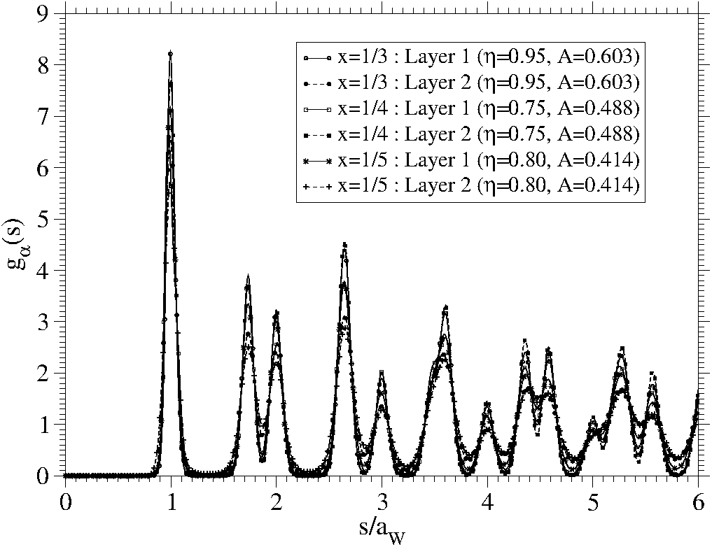
Figure 23: Correlation functions $g_{\alpha}(s)$, $\alpha=1,2$, for phases V_x as obtained in MC simulations at finite temperature, with the distances $s$ scaled by the respective $a_{i;{\rm W}}$-values. The correlation functions have been calculated for different state points and selected layers (as labeled).

We analyze here the scaling behaviour of the correlation functions $g_{\alpha}(s)$ with $\alpha=1,2$ (see the definition in. Eq. (13)), as observed in phase V_x. A relevant and appropriate length scale to represent the distance dependence of these correlations functions – independently of the particle densities $n_{1}$ and $n_{2}$ in each layer – are the respective lattice spacings of the hexagonal 2D Wigner crystal, $a_{i;{\rm W}}=(2/\sqrt{3}n_{i})^{1/2}$, $i=1,2$; for each layer the respective surface density is given by $n_{1}=(\sigma_{1}+\sigma_{2})(1-x)$ and $n_{2}=(\sigma_{1}+\sigma_{2})x$, while the total density for all particles projected onto the same plane is given by $n=n_{1}+n_{2}$. As explained in Section V, particles arrange in phase V_x in both layers as hexagonal 2D Wigner crystals, therefore the intralayer correlation functions have to fulfill in each of the layers a scaling law, imposed by the respective surface densities. More precisely, the rescaled intralayer correlation functions fulfill in phases V_x the relation

$$g_{1}\left(\frac{s}{a_{1;{\rm W}}};(1-x)^{1/2}\Gamma\right)\simeq g_{2}\left(\frac{s}{a_{2;{\rm W}}};x^{1/2}\Gamma\right)$$ (105)

where we have included the dependence of the correlation functions on the coupling constant $\Gamma$ (see Subsection II.6) to emphasize the surface density dependence in both layers.

Results shown in Fig. 23 verify the scaling law specified in Eq. (105): in this figure the correlation function $g_{\alpha}(s)$, with the distance $s$ appropriately scaled, are shown for several state points of phase V_x and selected layers (as labeled). For all these correlations functions, the first three peaks are located at $s=a_{i;{\rm W}}$, $s=\sqrt{3}\mbox{ }a_{i;{\rm W}}$, and $s=2a_{i;{\rm W}}$; the differences in the height and in the width of the peaks are due to the $\Gamma$-dependence. We could verify this scaling law of the intralayer correlation functions in all of our MC simulations performed for the phases V_x.

F.3 Further structural details and additional snapshots

This subsection contains a few snapshots of the full systems simulated in Monte Carlo simulations (Figs. 24 and 25) which do not belong into the main text; for the discussion we refer to Section VII.

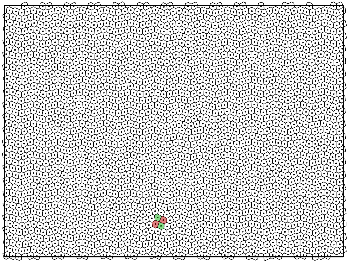
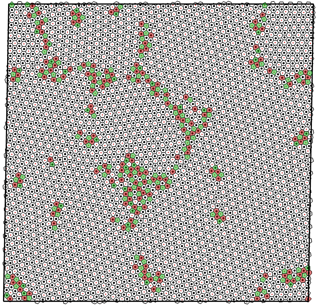
(a) (b) (c)

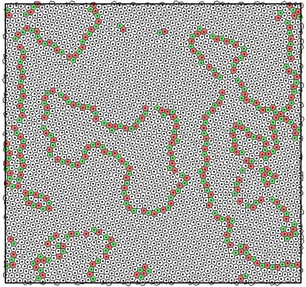
Figure 24: (Color online) Selected snapshots of the full systems as obtained in MC simulations, along with the related Voronoi constructions. The color code for the Voronoi cells is the following (color and number of edges): yellow (four), green (five), white (six), red (seven), and blue (eight). (a) Layer 1 of the DV_x phase ($x=3/7$, $\eta=0.68$, $A=0.814$); the Voronoi constructions have been performed only for the particles in layer 1 (in black). (b) phase H ($x=1/3$, $\eta=0.3$ and $A=0.771$); the Voronoi constructions have been performed for all particles projected onto the same plane, particles in layer 2 are shown in red. (c) Layer 1 of phase V_x, close to the transition to phase P₃ ($x=1/5$, $\eta=0.62$ and $A=0.466$).

(a) (b)

Figure 25: (color online) Structures I_x=1/4 observed in MC simulations within the domains $x=1/4$ and $x=1/5$. (a) Kagomé lattice of layer 1 in the phase I_x=1/4 ($\eta=0.10$ and $A=0.874$) as identified in the domain $x=1/4$. (b) Grains of phase I_x=1/4 ($\eta=0.28$, $A=0.67$) as identified in the domain $x=1/5$.

References

- (1) E.P. Wigner, Phys. Rev. 46, 1002 (1934).
- (2) C.C. Grimes and G. Adams, Phys. Rev. Lett. 42, 795 (1979).
- (3) D.C. Tsui, H.L. Stormer, and A.C. Gossard. Phys. Rev. Lett. 48, 1559 (1982).
- (4) J.P. Eisenstein and A.H. MacDonald, Nature 432, 691 (2004).
- (5) Zhihai Wang, Yong P. Chen, L.W. Engel, D.C. Tsui, E. Tutuc, and M. Shayegan, Phys. Rev. Lett. 99, 136804 (2007).
- (6) Zhihai Wang, Yong P. Chen, Han Zhu, L.W. Engel, D.C. Tsui, E. Tutuc, and M. Shayegan, Phys. Rev. B 85, 195408 (2012).
- (7) D. Zhang, X. Huang, W. Dietsche, K. von Klitzing, and J. H. Smet, Phys. Rev. Lett. 113, 076804 (2014).
- (8) D.S.L. Abergel and T. Chakraborty, Phys. Rev. Lett. 102, 056807 (2009).
- (9) G.E. Morfill and A.V. Ivlev, Rev. Mod. Phys. 81, 1353 (2009).
- (10) A. Pertsinidis and X.S. Ling, Phys. Rev. Lett. 87, 098303 (2001).
- (11) V.M. Bedanov and F.M. Peeters, Phys. Rev. B 49, 2667 (1994).
- (12) Yu.E. Lozovik, Usp. Fiz. Nauk 153, 356 (1987).
- (13) Yu.E. Lozovik and L.M. Pomirchy, Phys. Status Solidi B 161, K11 (1990).
- (14) Yu.E. Lozovik and V.A. Mandelshtam, Phys. Lett. A 145, 269 (1990).
- (15) Yu.E. Lozovik and V.A. Mandelshtam, Phys. Lett. A 165, 469 (1992).
- (16) F. Bolton and U. Rössler, Superlatt. Microstruct. 13, 139 (1993).
- (17) M. Baus and J.-P. Hansen, Phys. Rep. 80, 1 (1980).
- (18) E.A. Martinez. C.A. Muschik, P. Schindler, D. Nigg, A. Erhard, M. Heyl, P. Hauke, M. Dalmonte, T. Monz, P. Zoller, and R. Blatt, Nature 534, 516 (2016).
- (19) R. Blatt and C.F. Roos, Nat. Phys. 8, 277 (2012).
- (20) G. Goldoni and F.M. Peeters, Phys. Rev. B 53, 4591 (1996).
- (21) J.-J. Weis, D. Levesque, and S. Jorge, Phys. Rev. B 63, 045308 (2001).
- (22) V. Lobaskin and R. R. Netz, EPL 77, 36004 (2007).
- (23) E. C. Oǧuz, R. Messina, and H. Löwen, EPL 86, 28002 (2009).
- (24) L. Šamaj and E. Trizac, EPL 98, 36004 (2012).
- (25) L. Šamaj and E. Trizac, Phys. Rev. B 85, 205131 (2012).
- (26) T.B. Mitchell, J.J. Bollinger, D.H.E. Dubin, X.-P. Huang, W.M. Itano, and R.H. Baugham, Science 282, 1290 (1998).
- (27) D.H. Winkle and C.A. Murray, Phys. Rev. A 34, 562 (1986).
- (28) J.P. Eisenstein and A.H. MacDonald, Nature 432, 691 (2004).
- (29) The case is somewhat simple and of little interest, because we deal with ions that are all of the same charge. In this case, one plate repels them while the other is attractive, and structure I ensues. The interesting cases under study here are for and of the same sign, opposite to that of the point ions. Without loss of generality, we consider , and both , , to be positive.
- (30) S. Earnshaw, Trans. Cambridge Philos. Soc. 7, 97 (1842).
- (31) D.E. Goldberg, Genetic Algorithms in Search, Optimization, and Machine Learning, Addision-Wesley (Boston, MA, 1989).
- (32) D. Gottwald, G. Kahl, and C. Likos, J. Chem. Phys. 122, 204503, (2005)
- (33) M. Mazars, Phys. Rep. 500, 43 (2011).
- (34) J. Fornleitner, F. Lo Verso, G. Kahl, and C.N. Likos, Soft Matter 4, 480 (2008)
- (35) J. Fornleitner and G. Kahl, EPL 82, 18001 (2008)
- (36) G.J. Pauschenwein and G. Kahl, Soft Matter 4, 1396 (2008)
- (37) G. Doppelbauer, E. Bianchi, and G. Kahl, J. Phys. (Condens. Matter) 22, 104105 (2010)
- (38) G. Doppelbauer, E.G. Noya, E. Bianchi, and G. Kahl, Soft Matter 8 7768 (2012)
- (39) D. Frenkel and B. Smit, Understanding Molecular Simulation, Academic press (Amsterdam, 2001), second edition.
- (40) M.P. Allen and D.J. Tildesley, Computer Simulation of Liquids, Oxford (Oxford, 2017), second edition.
- (41) P.J. Steinhardt, D.R. Nelson, and M. Ronchetti, Phys. Rev. B 28, 784 (1983).
- (42) G. Zhang, F.H. Stillinger, and S. Torquato, Phys. Rev. E 92, 022119 (2015).
- (43) J. Gong, R.S. Newman, M. Engel, M. Zhao, F. Bian, S.C. Glotzer, and Z. Tang, Nat. Commun. 8, 14038 (2017).
- (44) S.C. Glotzer and M.J. Solomon, Nat. Mater. 6, 557 (2007).
- (45) E. Bianchi, P.D.J. van Oostrum, C.N. Likos, and G. Kahl, Curr. Opin. Coll. Int. Science 30, 18 (2017).
- (46) E. Bianchi, B. Capone, I. Coluzza, L. Rovigatti, and P.D.J. van Oostrum, Phys. Chem. Chem. Phys. 19, 19847 (2017).
- (47) J. Mikhael, J. Roth, L. Helden, and C. Bechinger, Nature 454, (501) (2008).
- (48) Q. Chen, S.C. Bae, and S. Granick, Nature 469, 381 (2011).
- (49) E. Bianchi, C.N. Likos, and G. Kahl, ACS Nano 7, 4657 (2013).
- (50) E. Bianchi, C.N. Likos, and G. Kahl, Nano Lett. 14, 3412 (2014).
- (51) M. Antlanger, G. Kahl, M. Mazars, L. Šamaj, and E. Trizac, Phys. Rev. Lett. 117, 118002 (2016).
- (52) R. Messina and H. Löwen, EPL 91, 146101 (2003).
- (53) R. D. Misra, Math. Proc. Cambridge Philos. Soc. 36, 173 (1940); M. Born and R. D. Misra, Math. Proc. Cambridge Philos. Soc. 36, 466 (1940).
- (54) R. Byrd, P. Lu, J. Nocedal, and C. Zhu, SIAM J. Scient. Stat. Comput. 16, 1190, (1995).
- (55) D. Wales and J. Doye, J. Phys. Chem. A 101, 5111, (1997).
- (56) M. Mazars, EPL 84, 55002 (2008).
- (57) A. Okabe, B. Boots, K. Sugihara, and S. Nok Chiu, Spatial Tessellations: Concepts and Applications of Voronoi Diagrams (John Wiley & Sons, Inc. - New York - 2000, Second Edition).
- (58) W. Mickel, S. C. Kapfer, G. E. Schröder-Turk, and K. Mecke, J. Chem. Phys. 138, 044501 (2013).
- (59) H. Leipold, E.A. Lazar, K.A. Brakke, and D.J. Srolovitz, J. Stat. Mech. 0443103 2016 (2016); ibid. 079901 2017 (2017).
- (60) M. Mazars, EPL 110, 26003 (2015).
- (61) With our code and for the choice of parameters for the Ewald method used in this study, CPU-times that are required to perform MC-cycles for a systems with particles typically amount to 48 CPU-hours on IBM IDataplex DX360 processors; this computer time also covers the numerical effort required for the Voronoi constructions Voronoi:Book which are performed after each MC-cycle.
- (62) I. J. Zucker, J. Math. Phys. 15, 187 (1974).
- (63) I. J. Zucker and M. M. Robertson, J. Phys. A 8, 874 (1975).
- (64) M. Antlanger, M. Mazars, L. Šamaj, G. Kahl, and E. Trizac, Mol. Phys. 112, 1336 (2014).
- (65) Moiré patterns are created by superposing two simple lattices. Depending on the commensurability and the relative orientation of the two lattices, highly complex patterns can emerge.
- (66) R. Messina, C. Holm, and K. Kremer, Phys. Rev. E 64, 021405 (2001).
- (67) M. Antlanger, G. Doppelbauer, and G. Kahl, J. Phys. (Condens. Matter) 23, 404206 (2011).
- (68) B. Grünbaum and G.C. Shephard, Tilings and Patterns (New York: Freeman, 1987, second edition).
- (69) In order to define these pathways, , suitable interpolating polynomials have been fixed, which are specified in Appendix F.
- (70) H. Leipold, E.A. Lazar, K.A. Brakke, and D.J. Srolovitz, J. Stat. Mech. 0443103 2016 (2016); ibid. 079901 2017 (2017).
- (71) P.M. Chaikin and T.C. Lubensky, Principles of condensed matter physics Cambridge University Press (Cambridge, 2013).
- (72) S.-K. Ma, Modern Theory of Critical Phenomena (Westview Press, New York, 1976).