A Framework for Planet Detection with Faint Light-curve Echoes

Abstract

A stellar flare can brighten a planet in orbit around its host star, producing a light curve with a faint echo. This echo, and others from subsequent flares, can lead to the planet’s discovery, revealing its orbital configuration and physical characteristics. A challenge is that an echo is faint relative to the flare and measurement noise. Here we use a method, based on autocorrelation function estimation, to extract faint planetary echoes from stellar flare light curves. A key component of our approach is that we compensate for planetary motion; measures of echo strength are then co-added into a strong signal. Using simple flare models in simulations, we explore the feasibility of this method with current technology for detecting planets around nearby M dwarfs. We also illustrate how our method can tightly constrain a planet’s orbital elements and the mass of its host star. This technique is most sensitive to giant planets within 0.1 au of active flare stars and offers new opportunities for planet discovery in orientations and configurations that are inaccessible with other planet search methods.

1 Introduction

Like a radar chirp or a sonar ping, a pulse of light from an astrophysical object allows us to glimpse the surrounding darkness. By tracking the light curve of a time-varying astrophysical source, we can extract the echo of such a pulse, looking for scattered light from things otherwise hidden (e.g., Rest et al., 2012). Examples include the discovery of rings and other features following supernova explosions (e.g., Crotts et al., 1989), and reverberation mapping of protoplanetary accretion disks around stars and gas in the vicinity of supermassive black holes (e.g., Horne et al., 1991; Peterson & Horne, 2004; Meng et al., 2016). Light echoes of stellar flares may potentially reveal the presence of planetary disks of dust/debris (Gaidos, 1994; Sugerman, 2003) and planets (Argyle, 1974; Matloff & Fennelly, 1976; Bromley, 1992; Clark, 2009; Mann, 2017; Sparks et al., 2018). Recently, Sparks et al evaluated additional discriminants of the scattered light, including fluorescence signatures and Doppler effects, thus bolstering the case for detecting echoes around M dwarfs.(Sparks et al., 2018) Echoes from multiple flare events from the same star change with the orbit of a planet and its physical properties, thus providing a new avenue for extracting orbital parameters(Argyle, 1974; Mann, 2017).

Detection of planetary echoes is challenging. However, if it can be accomplished, it nicely complements other planet detection methods. Transit surveys, although limited to edge-on systems, can provide planetary and stellar radii and estimates of orbital elements (e.g., Borucki et al., 2010; Mullally et al., 2015). Radial velocity studies (e.g., Mayor et al., 2011) also constrain planetary masses; when combined with transits, they set a gold standard for planet confirmation. Other methods, including microlensing (see Sumi et al., 2011) and direct detections (e.g., Marois et al., 2008; Janson et al., 2013), are sensitive to planets on distant orbits.

Planetary echoes provide a direct detection method for close-in planets that works irrespective of a viewer’s orientation, made possible only by the time-variability of their host. Figure 1 illustrates the sensitivity of these detection methods to planet size, orbital distance, and orientation relative to an observer.

A key to using planetary echoes for new detections, or as follow-up to known planetary systems, is repeat events. Like transits and radial velocity measurements, sampling a planet at various points along its orbit allows for reconstruction of orbital elements. In echo detection, differences in the arrival time of echoes can provide tight constraints on orbital elements and viewing angles. Because sets of echo delay times depend on physical distance and orbital period, the mass of the host star can also be accurately estimated. That echoes are photons reflected from the planet itself means that their strength depends on planet radius and albedo (atmospheric and surface composition) and orbital phase. Echo sets can arise from any viewing angle, but echo strengths fall off quickly with distance. Thus the method is most sensitive to giant planets inside 0.1 au for typical flare stars (Fig. 1). If combined with transits and radial velocity measurements, which provide separate constraints on stellar and planetary radii and masses, the possibility of using echoes to constrain the planet’s surface composition is greatly enhanced.

The ideal star for planetary echo detection has many strong, short outbursts. As a class, M dwarfs seem particularly well suited. A subset of these stars (the dMe) have tens of flares per day (e.g., Pettersen et al., 1986; Hawley et al., 2014; Davenport et al., 2016; Yang et al., 2017), and the contrast between the flare emission and the quiescent stellar light can be as high as $10^{4}$–$10^{5}$ (e.g., Schmidt et al., 2014, 2016). This combination — high flare frequency and strong flare contrast — make these stars, including AD Leonis (Bromley, 1992) and Proxima Cen (Sparks et al., 2018), excellent preliminary candidates for light echo detection. Furthermore, M dwarfs are the most common type of star in the galaxy(Ledrew, 2001), providing a very large number of potential observation targets.

Figure 1: Detection regimes for each leading exoplanet detection method, plotted in a cylindrical coordinate system with the semi-major axis as the radial coordinate, system orientation as the azimuthal coordinate, and planet size/mass as the depth coordinate (adapted from (Mann, 2017)). Transit is shown in green, radial velocity in yellow, direct imaging in red, and echo detection in blue. Echoes allow probing into inner solar systems viewed from any angle, which were previously very difficult to detect.

The detection of faint echoes is an extraordinary challenge, calling for a commitment of both collecting area and observing time. Observation of echoes from an exoplanet requires (i) analyzing a signal that is typically buried in the measurement noise, (ii) isolating the echo from the possibly complex flare tail and post-flare brightening activity, (iii) accounting for the probability that the exoplanet is in a favorable position relative to both the flare and Earth, and (iv) developing detection significance criteria. While the concepts motivating this ‘interstellar lidar’ are straightforward, there is no generalized approach available to enable demonstration.

Here, we propose a framework for exoplanet echo detection by statistical analysis of the autocorrelation signals of multiple high-contrast flare events measured at high cadence (typically 10 s or faster). Through simulations, we show that we are able to extract echoes and orbital and other parameters by additively building up a signal using data from a sufficiently large number of flares and, in most cases, can place confidence intervals on the data by using statistical analysis and resampling techniques. As we show here, even if echoes are not individually resolved in light curves, their signatures can rise above noise when combined together using assumptions about a planet’s orbit to account for variations in the echo delay time. In practice, confirmation of the presence of faint echoes and estimates of the planet’s orbital elements go hand in hand.

We organize this paper as follows. In §2, we review echo detection and describe the algorithms we use for selecting and processing flare light curves. Toward understanding the feasibility of our method, we also provide examples of successful planet detection and parameter extraction from mock flares. Then, in §3, we provide a framework for using faint echoes for planet discovery, with details for how to explore the inner regions of planetary systems by tracking flare activity. We consider the prospects of using this method for planet discovery or follow-up observations in §4 and we conclude in §5.

2 Feasibility of faint echo detection

In a flare event, some photons travel directly to an observer while others take a different route, scattering off the surface of a planet before heading to the observer. The difference in the light travel time is the echo delay. The strength of the echo depends on the relative orientation of the planet to the flare and the observer, as well as the absorption and phase characteristics of the planet. These two main characteristics of a planetary echo, delay time and strength, are illustrated in Figure 2. A face-on, circular orbit provides the simplest case with echoes of constant delay time, neglecting the spatial extent of the star and flare, and identical strength, neglecting native variability of the albedo. An edge-on observation of the same planet has echoes that are strongest when the planet is on the opposite side of the star; the echo delay time is longest there as well, equal to twice the delay time in the face-on case. When the planet is in a transiting configuration, there is no echo delay, and the echo strength vanishes. Intermediate viewing angles and planets on eccentric orbits give sets of echo time delays and strengths that encode orbital parameters. We begin setting up a framework for how to decode this information by examining the nature of individual flares and how to find faint echoes buried in them.

Figure 2: Schematic of a circular orbit is depicted at a perspective angle illustrating the orientation-dependent planetary echo from a flare event. The solid-line arrows represent the signal from the flare event; the dashed-line arrows represent the signal from the echo. The blue-line arrows travel to a face-on observer; the black-line arrows travel to an edge-on observer. The light travel time from the star to the exoplanet, $t_{1}\sim a/c$, remains constant for all orbital positions. The light travel time from the star to Earth, $t_{0}$, is assumed the same for all orientations. The exoplanet-Earth light travel time, $t_{2}$, is therefore the only parameter that depends on the orientation. The echo lag time, $\tau=t_{2}+t_{1}-t_{0}$, depends on the specific orientation. (a) When the exoplanet approaches inferior conjunction (the transit configuration), $\tau\rightarrow 0$ as $t_{2}\rightarrow t_{0}-t_{1}$. (b) When the exoplanet is observed near quadrature, the delay time is the light travel time from the star to the planet, $\tau\sim a/c$ as $t_{2}\sim t_{0}$, which is equivalent for edge-on and face-on orientation. (c) When the exoplanet approaches superior conjunction, $\tau\rightarrow 2a/c$ as $t_{2}\rightarrow t_{0}+t_{1}$. (d) The relative echo lag and approximate exoplanet visibility as a function of orbital phase and orientation for a circular orbit.

2.1 Flare Analysis

Flare events typically exhibit common characteristics (Pettersen et al., 1986; Loyd & France, 2014; Kowalski et al., 2016): a rapid rise to peak brightness that can be seconds or less, followed by a slower decay characterized by a time $\tau_{1/2}$, the full-width at half-maximum of the flare, that can range from seconds to minutes. Finally, a gradual, more slowly dissipating phase can persist from under a minute to hours. For echo detection, it is simplest to work with shorter-lived flares, for which the early, rapidly varying part of the flare light curve vanishes by the time the echo arrives at the detector. Echoes from a planet within 0.1 au of the host star have delay times that are typically seconds to minutes, depending on orientation. Thus, at least a subset of flares may be well-suited to echo detection.

For echo detection of a planet around a flare star, we first consider an observed light curve for a single flare event. To evaluate detection bounds, we assume that the flare is an isotropic point source, impulsive relative to the cadence, appearing in one bin only, producing a signal ${\cal{F}}_{p}$ (e.g., in units of photon counts) above the constant stellar background rate, $Q$. The r.m.s. noise level in the continuum is $\cal{N}_{\text{rms}}$ and $s_{min}$ is the minimum signal-to-noise ratio that the astronomer has determined is acceptable for the detection experiment (with the practical constraint $s_{min}\geq 1$), giving a detection regime of

$$\epsilon \gtrsim \frac{s_{min}\cal{N}_{\text{rms}}}{{\cal{F}}_{p}}\approx\frac{s_{min}\sqrt{Q\Delta t}}{{\cal{F}}_{p}}$$ (1)

where $\epsilon$ is the exoplanet-star (echo-flare) contrast ratio, the integrated time bin is of duration $\Delta t$, and the second line assumes that the noise comes from counting statistics in the continuum integrated in a time bin. However, flares typically have a broad tail and cannot be easily summed in a single time bin.

To provide a method for more realistic flares, we consider the typical structure of a flare measurement. The light curve, $L(t)$ (in units of photon counts per second, typically), has contributions from a single flare with flux $F(t)$, its echo, and measurement noise $N(t)$:

$$L(t)=Q+F(t)+\epsilon F(t-\tau_{\text{echo}})+N(t),$$ (2)

where $\epsilon=p\phi(\alpha)(R^{2}/a^{2})$ is the approximate echo contrast of an exoplanet with semi-major axis $a$, geometric albedo $p$, radius $R$, and phase function $\phi(\alpha)$, and $\tau_{\text{echo}}$ is the echo delay, both of which depend on the geometry of the star (where the flare presumably originates), the planet (responsible for the echo), and the position of the observer. Figure 3 illustrates an idealized flare light curve with an echo whose strength ($\epsilon=10^{-5}$) is comparable to the noise level.

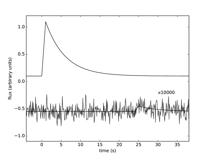
Figure 3: Simulated flare with an echo. The echo amplitude and synthetic Gaussian noise, visible in the lower curve (shifted downward and scaled with a multiplicative factor for clarity) are both at the level of $10^{-5}$ relative to the flare amplitude.

The extraction of the faint echo in the presence of noise is a problem in signal processing. Since a flare echo is just the time-delayed repetition of a flare, a good tool for extracting the echo is the autocorrelation function (Argyle, 1974; Bromley, 1992). This statistical tool provides a sensitive measure of the similarity of a given signal to itself as a function of time delay. A detailed description of the autocorrelation analysis is provided in Appendix A.

We caution that, even in ideal scenarios with large echo contrast, it may be difficult to discern a flare with a planetary echo from a multi-peaked flare. The autocorrelation function might not yield a distinction between the two cases. Furthermore, a flare may not produce an echo at all, as when a flare is localized on the stellar surface, but on the opposite side relative to the planet. These challenges associated with realistic observing conditions are considered in the following sections.

2.2 Observational requirements for echo detection

To provide meaningful detection criteria, even in scenarios with large signal-to-noise ratios, multiple flares are needed to rule out false alarms like multiple peaks in the same flare event. When a planet is on a circular orbit and observed face-on, all echoes occur with the same delay time, and so add together to strengthen the signal. In general, the planet’s orbital motion causes echoes in a set of flares to occur at different times, but we can compensate for this effect so that echo signals in the correlation function are aligned, adding together at some common lag (see §2.3 below). Then, the total echo signal grows linearly with the number of flares, $N_{\text{f}}$, while the noise increases as the square root of this number. This linear dependence may change depending on the flare brightness distribution; see for example (Sparks et al., 2018). Thus, the typical echo contrast required for detection falls off with $N_{\text{f}}$ as

$$\epsilon \gtrsim \frac{s_{min}}{\langle{\cal{F}}_{p}\rangle}\sqrt{\frac{Q\Delta t}{N_{\text{f}}}},$$ (3)

which follows from Eq. 1, with $\langle{\cal{F}}_{p}\rangle$ as the average flare strength. To obtain approximate observation times required to detect an exoplanet, we define $N_{f}=\nu_{f}t_{obs}$, where $\nu_{f}$ is the flare frequency and $t_{obs}$ the total observation time and consider a Lambertian planet phase function(Traub & Oppenheimer, 2010) to obtain:

$$t_{obs}\gtrsim\frac{s_{min}^{2}Q\Delta t}{\nu_{f}\langle{\cal{F}}_{p}\rangle^{2}\epsilon^{2}}=\frac{s_{min}^{2}Q\Delta t}{\nu_{f}\langle{\cal{F}}_{p}\rangle^{2}}\frac{\pi^{2}a^{4}}{p^{2}R^{4}}$$ (4)

where the $\pi^{2}$ term arises from viewing the planet from a face-on configuration, see Eq. B1. In reality, this factor may need to be multiplied by 2 to account for half the flares missing the exoplanet, presumably occurring on the opposite side of the star from the planet, but still being observed by our telescope. From Equation (4), we see that the time required to monitor the star goes as the inverse square of the exoplanet-star contrast, $\epsilon$, which goes as the inverse square of the distance from the star. Hence, the monitoring time depends on the star-planet separation to the fourth power. Therefore, stellar flare echoes are best detected from exoplanets that are near to their host star.

To demonstrate the feasibility of using this technique under ideal conditions, we produce a set of proof-of-concept simulations. First, we consider impulse flares that occur within a single time bin, and set 50% of the flares to miss the exoplanet, which systematically de-correlates the signal. We select U-band magnitude $m_{U}=12$ with flares that result in $\Delta m_{U}=-2$, which are parameters relevant to many M dwarfs. We then generate an echo consistent with a hot Jupiter at 0.03 au, $R=2R_{J}$, albedo of 0.9, viewed in a face-on circular orbital configuration. To quantify the results, we calculate the signal that would be observed with a 2 m diameter telescope with a 2 s integration time and then add counting noise with the numpy random.poisson function(Oliphant, 2006). The flares are assumed to be non-overlapping in time. The resulting data have an echo-magnitude/mean counting-noise (signal-to-noise) ratio of $s=1.0$ for each flare. Under these conditions, using Eq. 4, the predicted number of flares required to achieve $s=\{3,5,10\}$ is $\{27,75,303\}$. Figure 4 provides an example of a simulated light curve from this experiment with and without noise and its detrended correlation function for increasing numbers of flares.

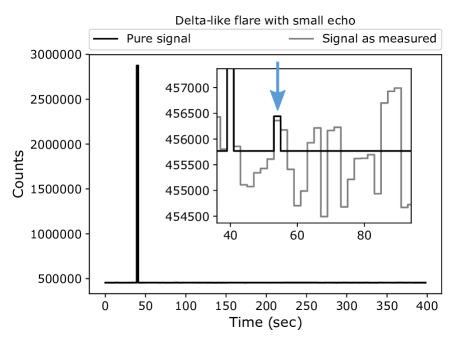
(a) Simulated light curve with and without noise.

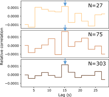
(b) Detrended correlation function for increasing numbers of flares.

Figure 4: The light curve and correlation function for ideal impulsive flares from a star with $m_{U}=12$, with flare magnitude $\Delta m_{U}=-2$, observed by a 2-m diameter telescope with a 2 s integration time. An echo comes from a planet at $a=0.03$ au, on face-on circular orbit, with $R=2R_{J}$ and $p=0.9$. The resulting echo delay time is 15 seconds. The flares are identical, but the noise profiles are generated independently for each sample. The plots illustrate how multiple flare events are essential for faint echoes to produce a significant imprint in the correlation function. With 27 flares, the echo corresponds to an insignificant peak in the correlation function. When 75 flares are included, the echo is the largest peak in the correlation function, but it is of similar magnitude to some other false peaks.

Under real observing conditions, the nearly face-on circular orbit case appears to be the most promising configuration because all echoes will accumulate within one or two time bins, avoiding the need to align echo lags. Unfortunately, a signal accumulating within a common lag bin is also a noise condition that can be expected from real instrumentation(Mann, 2017). Therefore, using these data sets, we (i) analyze the direct autocorrelation signal, and (ii) perform a statistical hypothesis testing experiment that is motivated by the system phenomenology. Because half of the flares are hidden from the hypothetical planet and will not produce echoes, we would expect a bimodal distribution of the correlation values at the time of the lag, and a unimodal distribution elsewhere when there is no echo. These two cases, a null hypothesis of no echo with a unimodal distribution and a positive detection hypothesis of a bimodal distribution, are now open to the vast toolkits available from statistical analysis. For instance, with a sufficiently large dataset, the detection case will typically manifest itself as having a larger variance and smaller kurtosis and discernible differences in the kernel density estimation.

In Figure 4, we examine direct autocorrelation echo detection in the model where a planet is observed face-on, using data sets with 27, 75, and 303 mock flares. We find that the autocorrelation time lag corresponding to the echo, indicated with an arrow, produces a strong signal, but is not convincingly distinct from the background until the 303 flare case. Then, we explore a hypothesis testing analysis: instead of summing the autocorrelation values at each time lag, we compute kernel density estimates of the autocorrelation functions at each time lag, using a normal kernel with a bandwidth determined by Silverman’s (1986) rule of thumb. The left side of Figure 5 shows these estimates at the time lag equal to the echo delay time (15 s), and at two different lags for which the echo signal would not contribute to the autocorrelation function. With $N=27$ mock flares contributing to the correlation function, the echo case is not meaningfully discernible from the no-echo case. For the $N=75$ and $N=303$ cases, there is a difference in the mean of the distributions and the shape of the tail of the kernel density estimate.

From the kernel density estimate shown in Fig. 5, we calculate the cumulative distribution function and fit it with the cumulative distribution function of a bi-Gaussian model where both Gaussians are assigned the same amplitude and width, consistent with the model’s anticipated phenomenology. In each case, one Gaussian’s mean is allowed to float, while the other is ’fixed’ at the mean of the correlation values in adjacent time-lag bins. In more general models, the fixed position can be selected from a detrended background curve, for example. The model fit thus has two free parameters: a Gaussian mean and the width of both Gaussians. We perform the fitting with the SciPy optimize.curve_fit routine(Jones et al., 2001). The fitted mean position at each time lag is shown in the plots on the right side of Fig. 5 as orange triangles and the positions of the fixed Gaussian is shown as an upside down triangle. These values are then compared to the raw autocorrelation values, shown as a horizontal black bar and taken from the data in Fig. 4.

Toward producing meaningful confidence limits, we resample the correlation values with replacement (a statistical method known as bootstrapping) and re-calculate the two-Gaussian model fit for each resampled distribution. We use 1000 resampled sets and evaluate the upper and lower confidence intervals with Python’s numpy percentile function.(Oliphant, 2006) The light orange bars in Figure 5 show the position of the 98% confidence values. When the bars from the floating Gaussian mean overlaps the bars from the fixed Gaussian mean, we say that there in insufficient information to claim a detection event. This is the case for all time lags in the N=27 case. When a larger number of flares are observed, the 98% confidence interval of the fitted Gaussian is far enough away from those of the fixed Gaussian such that there is no overlap between the two at only one time, 15 s. Here, we can say that this model indicates an echo detection event with 98% confidence. This occurs in the N=75 case and is more significant in the N=303 case. These detection events correctly correspond to the time and magnitude of the synthetic echo; the fitted Gaussian mean is close to the exact solution (plus sign in Figure 5).

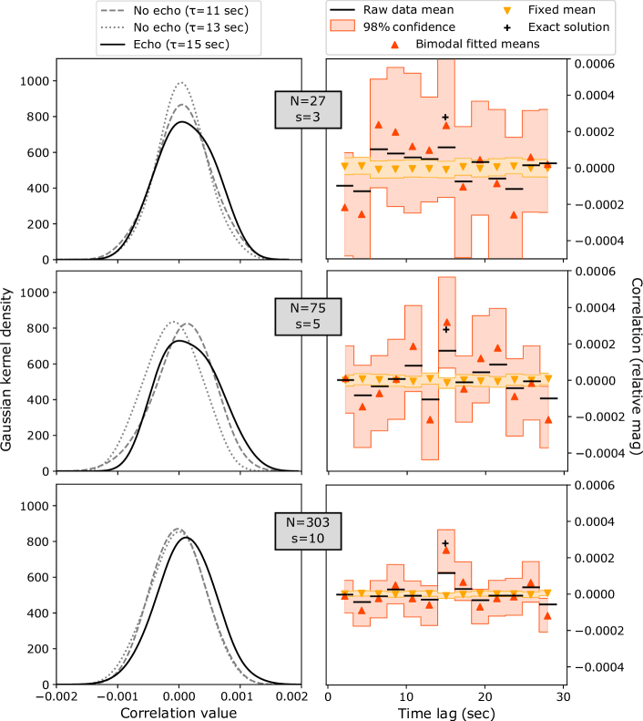
Figure 5: (Left) Gaussian kernel density estimates at the time of the echo and at two times without echoes. (Right) Bi-Gaussian fits of the correlation data for $N=\{27,75,303\}$ flares with $R=2R_{J}$ (same dataset shown in Fig. 4). The bimodal model consists of two identical Gaussian profiles, where one is fixed at a location consistent with no echo signal, and the other is allowed to float. While visibly subtle, the bimodality of the kernel density estimate proved to be quantitatively robust under bootstrap analysis. The location of the floating Gaussian mean becomes distinct from the fixed one at better than 98% confidence level at the lag equal to the echo delay time in the cases with $N=75$ and $303$. The parameter $s\sim\sqrt{N}$ indicates the strength of the echo contributions in each data set.

Given the high flare rates for M dwarfs, it should be plausible to select only the most impulsive flares and use them for such an analysis. For many stars, this will result in more than one useful datum per day, though additional detailed high-cadence measurements are necessary to say quantitatively how many useful flares can be expected for a given star class.

2.3 Echo detection with planetary motion

In the more general configurations when a planet’s orbit is not viewed face-on, the echo delay times may be different for each flare. If the echoes are buried in noise, then their signals cannot be fruitfully combined unless the true echo delay times are known. We can make progress by modeling the planet’s orbit and calculating echo delays accordingly. The relevant parameters are the host star mass, $M$, and the planet’s Keplerian orbital elements $a$, $e$, and $M_{0}$, where $a$ is the semimajor axis, $e$ is the orbital eccentricity, and $M_{0}$ is the mean anomaly at some reference time $T_{0}$. The echo delay will also depend on spherical polar viewing angles $\theta_{v}$ and $\phi_{v}$, such that $\theta_{v}=0$ mean a face-on view, while $\theta_{v}=90^{\circ}$ and $\phi_{v}=0$ means the planet is transiting the star at periastron. With these parameters (six in total, counting the stellar mass), and assuming a point-like star, we can calculate an echo delay time for any orientation and orbital phase using the equation for a constant-delay ellipsoid, borrowed from radar theory:

$$\tau_{\text{echo}}=\left(|\vec{r}|-\vec{r}\cdot\hat{e}_{\text{obs}}\right)/c,$$ (5)

where $\vec{r}$ is the position of the planet at the time of a flare, $\hat{e}_{\text{obs}}(\theta_{v},\phi_{v})$ is a unit vector pointing at the observer from the host star, and $c$ is the speed of light.

Figure 6 shows examples of how echo delay times and echo strengths depend on the orbital phase for various eccentricities and viewing angles. For the modest eccentricities considered here ($e\leq 0.2$), changes in viewing angle produce the most significant variations in delay times and echo strength. For example, a planet viewed nearly edge-on and from the opposite side of the star relative to the observer produces a strong echo with a large delay (twice that of a face-on view). As the planet moves between the observer and the star, the delay time decreases, and the echo strength drops, like the brightness of a waning moon. We show several more examples in Appendix B.

Figure 6: Echo delay time lag(Mann, 2017; Sparks et al., 2018) (top row) and star-exoplanet contrast ratio observed from Earth (bottom row) from a planet with $R=2R_{J}$, albedo of 0.9 at 0.03 au for eccentricities $\{0,0.05,0.1,0.15,0.2\}$ (darker lines correspond to higher eccentricities) for different inclination angles relative to Earth (face-on view is on the left, transit view is on the right). In these scenarios the viewer is nearest to the planet’s apoastron location. Eccentricity plays a more significant role for the nearly face-on configurations ($0-30^{\circ}$) where the differences in the exoplanet-star separation drives differences in the echo lag. For more extreme inclination angles, ($30-90^{\circ}$) the viewing angle drives most of the variation in both the time lag of an echo following a flare, and the star-exoplanet contrast. For example, in the face-on case, the the echo time lag is maximized when the exoplanet is furthest from the star ($t/T=0.5$ in this figure), but by a $30^{\circ}$ inclination angle, the time lag is actually minimized when the exoplanet is furthest from the star. This peculiarity arises because of the specific viewing angle relative to the planet’s apoastron location: despite being at its furthest distance from the star, it aligns closer and closer to the view of Earth with increasing viewing angle, reducing the echo lag to zero. Note that, using a combination of both lag time and echo contrast, we can distinguish between each case, despite the similarities of individual curves as a function of orbital phase.

Figure 7 provides an example of the autocorrelation function of a mock impulsive flare with an echo (see Fig. 3), along with sums of such functions from multiple flares with echoes from a planet on a Keplerian orbit. We pick the stellar mass, orbital elements, and viewing angles to calculate echo delays ($M=0.3\,{\rm M_{\odot}}$, $a=0.05$ au, $e=0.1$ and $M_{0}=70^{\circ}$ (relative to a fiducial starting time), $\theta_{v}=20^{\circ}$, with $\phi_{v}=60^{\circ}$). In our mock data, there are 100 flares, with onset times drawn at random over an interval that spans 10 planetary orbits, about 75 days. For each flare, we assume a linear rise in luminosity, and an exponential tail with a $\tau_{1/2}$ lognormally distributed about 3 s (e.g., Fig. 3); the rise times are 20% of the decay time up to a maximum of 1 s. In the mock data used to make Figure 7, the planet is moving, hence the echo lags are all different. Adding the raw autocorrelation functions together fails to reveal a compelling echo signature. When the autocorrelation functions are shifted so that the echo signals are aligned at a common lag, a strong peak emerges. In this flare catalog, the intrinsic flare brightness and the echo strength are held fixed from flare to flare, every flare lights up the exoplanet, and each flare is weighted equally. We then add noise in the form of independent Gaussian random variables, with the goal of mimicking counting noise. Both the echo strength and the r.m.s. noise are at a level of $10^{-5}$ relative to the flare amplitude. The purpose of these simulations is to test the feasibility of detection algorithms. To produce a more realistic catalog of flares, it would be required to include variability of flare amplitudes and phase-dependent planet albedo.(Russell, 1916)

Figure 7: The correlation signal of a set of mock flare echoes, similar to the one shown in Fig. 3, from a planet on a close, mildly eccentric orbit ($a=0.05$ au and $e=0.1$). The mock dataset contains 100 flares, all with echoes. The lower curve (offset vertically for clarity) is the correlator of a single flare; no trace of an echo is visible. The middle curve is the sum of all 100 correlators, which also shows little sign of any echoes. The strong peak in the upper correlator arises, despite that the echoes are buried in the individual light curves, because the lags of the individual correlators are adjusted to align the echo peaks at a lag equal to the average echo delay time ($a/c$). Thus, it is essential to compensate for the variation in delay time that arises from planetary motion.

With sufficiently long observations with adequately high signal-to-noise, we have found that periodogram analysis, such as period folding and Lomb-Scargle plots, can isolate the echo signal (see Appendix B). To be effective, however, these approaches require sufficient signal within a single lag bin to rise above the noise. For weaker signals, it is necessary to align the echo correlator lag to build up an echo signature. So we must systematically search through echo delay parameters to compensate for a planet’s motion. We return to this problem below. Meanwhile, we consider how the planet’s orbit affects the nature of echoes that may be observed.

To proceed beyond the circular orbit problem, we require the six parameters listed above to determine echo delays from a planet in Keplerian motion. Since we do not, in general, have a priori knowledge of these parameters — even the stellar mass may not be well constrained — we must search for them somehow, a task that is computationally daunting. Thus, we briefly explore a reduced parameterization of an echo delay by assuming that it varies sinusoidally in time (cf. Eq. B2):

$$\tau_{\text{echo}}=A\sin\big{(}2\pi\frac{t}{T}-P\big{)}+D,$$ (6)

where amplitude $A$, period $T$, phase $P$, and mean delay time $D$ are constants. This assumption is motivated by the sine-like structure of the lag-orbit plot for many orbital configurations (see Fig. 6 and Appendix B for several examples). The advantage of this parameterization is that the search space is 4D. Furthermore, we can substantially limit the search space since some of these parameters are related through physical conditions: For example, $A\leq D$, which intuitively means that the echo must always occur after the flare. Also $D$ (related to the mean distance to the planet) and $T$ (the orbital period) are related, so that one may be constrained by the other using Kepler’s third law, along with the uncertainty of the stellar mass.

Figure 8 illustrates the 4D search where we align the 100 individual correlation functions so that the peaks of the correlators would match if the echo delay were given by equation (6) for a given choice of $(A,T,P,D)$. Because a goal will be to work with noisy data such that the echo signal-to-noise is unity or less, we do not just add the aligned correlation functions. Instead, we apply a measure — the echo correlator strength $\mathcal{S}$ — that responds to a peak at the right lag, and the expected shape of the correlation function for each flare echo in the vicinity of the peak (which we know from the shape of the flare’s correlation function near zero lag). We define one prescription for $\mathcal{S}$ in Appendix C; We discuss several other possibilities below. Figure 8 maps out $\mathcal{S}$ in slices in the parameter space that contains the peak value. The strongest peak is close to the expected values, validating the approach. Once a strong value of the echo correlator strength, $\mathcal{S}$, has been determined, it is then possible to apply a statistical analysis, such as that from §2.2, to produce confidence intervals.

Figure 8: Maps of the echo correlator strength ($\mathcal{S}$) from a set of simulated flares (see text and Fig. 7). Each panel is a slice of a 4D parameter space that contains the peak value of $\mathcal{S}$. The left plot is the echo correlator strength as a function of delay variation amplitude ($A$) and phase ($P$), while the right plot shows variations of $\mathcal{S}$ with orbital period ($T$) and the mean lag/echo delay time ($D$). The peak of $\mathcal{S}$ lands very close to the expected values $(A,T,P,D)\approx(8.5\ \text{s},7.5\ \text{s},210^{\circ},25\ \text{s})$.

The next step is to generalize our search to any orbital configuration. We begin with the stellar mass ($M$) as a parameter. This is needed to relate the orbital period and the orbital distance, which are otherwise formally distinct in the calculation of the echo delay. We determine the range of mass values to search from the star’s spectral type by assuming an uncertainty of 10% in $M$. If the star was observed to have a bound stellar or planetary partner, we would adopt the dynamical mass estimate instead. For each mass choice, we allow semimajor axis, eccentricity, and viewing angles to vary. We focus on inner solar system planets, so we take $a<0.1$ au, $e<0.2$ as suggested by Han et al. (2014). We search the full range of possible orbital phase and viewing angles. Our implementation of the method uses a mixture of Python scripts and parallel C++/MPI code. The former does the data processing, while the latter performs the grid-based search of billions of points.

In Figure 9, we show maps of echo correlator strength in slices of the 6D parameter space ($M,a,e,M_{0},\theta_{v},\phi_{v}$) that contain the maximum value of $\mathcal{S}$. The peak value of $\mathcal{S}$ is close to its expected location; uncertainties derived from examining the region around the peak suggest that our method and choice of $\mathcal{S}$ is adequate for constraining the true orbital parameters.

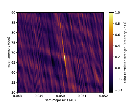
Figure 9: Maps of the echo correlator strength from the set of simulated flares illustrated in Figure 7, with echoes from a planet with orbital parameters $(a,e,M_{0},\theta_{v},\phi_{v})$ set to $(0.05~{}\text{au},0.1,70^{\circ},20^{\circ},60^{\circ})$. The panels on are drawn from three billion unique samples of all five parameters and stellar mass (0.3 $\rm M_{\odot}$). The peaks are near the true parameter values.

This brute-force, 6D search method is an acknowledgment that finding the true orbital elements and observer orientation is a needle-in-a-haystack problem: for the correct choice of parameters, and for a small region surrounding that point the parameter space, all the echoes line up in the estimation. For all other choices of $\mathcal{S}$ they do not (see Figure 7). Thus a downhill search method will not be successful, except if a search is started very close to the true orbital parameters. In contrast, the dense, grid-based search demonstrated here will eventually find the true orbital parameters.

Initially, we may use the vast majority of points in our parameter search spaces that incorrectly align the echo delay time to derive noise limits in a “hit-miss” approach. Because the vast majority of all fitting attempts are misaligned measurements, they sample a large number of different lag configurations. Figure 10 compares $\mathcal{S}$ from mock noisy data in a broad 6D search, both with and without echoes. The comparison shows that the incorrectly aligned $\mathcal{S}$ values serve to sample the noise distribution, even though they are derived from data with echoes. This approach is not necessarily statistically unbiased because the samples here are correlated by orbital dynamics and their order of observation. Nonetheless, Figure 10 suggests that, by omitting the region in the search space near a candidate echo signal, we can obtain a useful estimate of the one-point background distribution from which we may derive the statistical significance of a detection.

Figure 10: Histograms of echo correlation strength measure $\mathcal{S}$. The dark histogram is from our set of 100 mock flares with echoes, while the light curve is from mock data with no echoes. The histograms compare well at low-$\mathcal{S}$ values, as in a lag-resampling analysis, and as reminiscent of the bimodal analysis in Fig. 5.

In our simulated data, the largest peak correctly corresponds to the signal produced by the exoplanet, and the histogram of all echo correlators (Figure 10) shows a distinct knee in the distribution only when an echo is present. However, we acknowledge that additional work will be required for echo detection to approach the rigor of existing detection methodologies. For example, in practice each flare will be unique, so some multi-peaked flares or significant post-flare brightening events may generate a significant correlation signal at a given time lag. While it may be tempting to lean heavily on a small number of extreme events that produce a strong signal, we caution that these outliers require special handling. To reduce experimenter bias, there are outlier rejection methods in the field of statistics that will likely play a role in any substantive discovery claim. For example, the ‘jackknife’ or leave-p-out methods are subsampling methods that leave out samples, then recompute the result to see how it changes–the calculation is repeated for each subsample permutation. If a detection event is only present when a small set of the flares are included in the complete dataset, this would indicate that the effective sample size is much smaller than implied by the total number of flares collected and could call the result into question, depending on the specifics of the analysis.

One method we believe is promising for better identifying confidence intervals is lag resampling. In both the 4D and 6D search models, excepting the face-on circular orbital case, the lag and echo contrast values change throughout the orbit. Under the null hypothesis of no exoplanets, it should not matter if you reorder all of the flares. If there is an exoplanet, then reordering the flares will scramble the time lags and they will no longer add up coherently—the signal will be lost. Therefore, by resampling the order of the flares with replacement (bootstrapping), it is possible to quantify how often a given detection magnitude occurs. In performing this analysis, it is important to quantify the correlation of the resample: exchanging two flares that are co-added into the same lag bin will not resample the distribution. This lag resampling process can initially be performed just for the volume around the detection candidate. However, in sampling an enormous 6D parameter space, there is always the concern of discovering a spurious correlation that might arise from data dredging. Thus, to confirm any detection candidate, we suggest a full 6D bootstrap search of a resampled flare catalog to determine how likely false needles of the same magnitude would be discovered in the 6D haystack. A definitive exoplanet echo claim will not only require a large amount of data, but also an effort from the astronomy community to develop and agree on rigorous detection criteria. We hope that these flare models and simulation results motivate the beginning of that effort.

3 A framework for planet discovery

The feasibility studies performed in §2 indicate that it is challenging, though possible, to detect otherwise invisible exoplanets by their echoes. We therefore propose a generalized framework for the detection of planets from faint stellar flare echoes that involves a combination of signal processing and orbital estimation. The following steps provide an overview, while details of our demonstration implementation are provided in Appendix C.

Acquire data.

The most useful data will have a large flare signal, a high exoplanet albedo, and a low background signal. Also the cadence must be short, less than $\sim$10 s, by virtue of the short light-travel time for close-in planets. While the majority of energy produced during a flare is often in the visible band, and stellar variability and exoplanet albedo are chromatic, the U-band appears to be most promising general choice because of the consistently small background signal, particularly for M dwarfs (Bromley, 1992; Kowalski et al., 2016, and references therein). Beyond photometry, it is known that flare emission from different lines and parts of the spectrum is not always synchronized: some spectral signatures may lag others and evolve differently on a timescale relevant to echo detection, which depends on the specific phenomenology of the star and the flare (Klocová et al., 2017, for example). Running a cross-correlation on these signatures, often referred to as photoreverberation mapping, would then reveal a lag associated with the star’s phenomenology, not with an echo. On the other hand, if each spectral line can be linked to a known flare-exoplanet phenomenon, such as fluorescence, then it may be possible to use these signatures to greatly improve the detectability(Sparks et al., 2018). To exploit multispectral data using this manuscript’s framework, for all reflected light spectral signatures, each band’s light curve’s autocorrelation signal will be synchronized in the lag domain, even if a given band has an arbitrary lag relative to the others. Summing their autocorrelation signals can then further reduce the noise and uncertainty associated with a single flare event, though we have not explored the details of multiband autocorrelation in this study.

Process the light curve.

High-pass filtering, background subtraction, and detrending are essential to extraction of faint echoes in individual flares. Higher-level processing of sets of flare light curves can reveal additional information about active regions, such as star spots, and reveal possible star-orientations, rotation rates, and even differential rotation rates. These parameters can be fed into models to assist in estimating star mass, for instance. Additionally, when only a limited number of active regions are present, it becomes plausible to predict which hemisphere around the star is illuminated by a flare. This additional information can be used as a ‘stellar lock-in amplifier,’ which could downweight flares that miss the exoplanet. In general, this will knock down the noise much faster than histogram analysis, but is only viable when the star is cooperative.

Generate flare catalogs.

This step is to identify and select flare events and assign weights according to measures of quality, including flare strength and temporal structure or complexity. Strong, delta-function flares are ideal, but broader, weaker flares can also produce echoes. In practice, each flare is assigned a weight; the flare strength may be a major component of the weight, but other factors can include a flare’s width and structure, estimated by a frequency-domain analysis of the flare to identify the time-frequency bandwidth. We also recommend evaluating down-weighting any flares which exhibit detectable microflaring after the main pulse. While this may sound like a recipe for removing the exact data being sought, it is important to note that for most telescopes, particularly those under 10 m, the echoes will be near or below the noise level. In practice, the astronomer can compute a threshold detectability for a given time lag using Eq. 1 and earlier work(Bromley, 1992) based on the specific observing conditions, and tag post-flare events above an appropriately optimistic threshold for potential masking. This list is not exhaustive of weight possibilities; see the more detailed discussion in Appendix D.

Estimate autocorrelation functions.

The autocorrelation calculation is straightforward using discrete convolution routines. However, it is often necessary to detrend the autocorrelation function. Because flares have a long tail, they can introduce curves to the autocorrelation, and the echo will be a small bump riding on its back. In simulations, we successfully reduced this tail in a variety of ways, including linear detrending, fitting a cubic polynomial to the logarithm of the curve, and linear Savizky-Golay filtering. The optimal method typically depends on the flare structure.

Calculate echo correlator strength.

The autocorrelation curve signal strength will depend on the amplitude and detailed profile of the flare light curve. However, as the echo will essentially be an exact replica of the flare, its autocorrelation will also be a replica of the flare’s autocorrelation. Therefore, one means of calculating the echo strength is to extract the central peak of the correlator itself and convert it into a template for detection strength. The detection strength parameter is maximized when it is customized for each flare based on that flare’s structure, so the use of the autocorrelator itself is a self-adjusting, optimally ‘cusped’ template. Other templates include analytical filters such top-hat, triangle, or Savizky-Golay 2nd derivative filters—these are often tuned based on the width of the flare under analysis. After producing the detection template, it is convolved with the correlator, resulting in a detection probability vector. A discussion of this choice of echo correlator strength is given in Appendix C.

This process is performed for each flare, resulting in a detection matrix that can be readily indexed for the multi-dimensional search process. As the values approach zero-lag, which corresponds to a time only moments after the flare, it is useful to de-weight the signal because it can be strongly influenced by edge effects.

Search for echo candidates.

A first rapid search for echo candidates can use autocorrelation function estimates from the flare catalog to identify any high signal-to-noise events, or estimate any set of echoes that appear at constant lag. Next, Lomb-Scargle periodogram analysis provides a low-overhead analysis of the data, to identify any potential high signal-to-noise candidates that are not necessarily at constant lag. Beyond these glimpses into the data, it is necessary to align the detection strength parameters to the correct lag delay. Therefore, we choose plausible ranges of stellar mass, a planet’s orbital elements, and viewing parameters. For each set of values, we calculate time lags and extract echo correlator strengths from the flare catalog. The resulting list of strengths is then summed; if this result exceeds a threshold, it is flagged as a potential hit for detection confidence analysis. An alternative approach can make use of an explicit model for a planet and its expected echo correlator strength, which is compared to data using maximum likelihood analysis. This method may help eliminate false positives from microflaring.

We note that there are some orbital and viewing configurations that lead to degeneracies, at least in the predicted lag times. For instance, when the argument of the periapsis is pointing away from Earth, then orbits with $e=\sin{\theta_{v}}$ can also have a constant lag, similar to a face-on circular orbit. However, this degeneracy can be broken if we model the echo strength as a function of orbital phase. Here again, a maximum likelihood approach can help.

Determine detection confidence intervals.

Two means of identifying true detection events based on confidence levels include hit-miss distribution analysis and lag resampling, as described above. The idea is to build up a model of the noise distribution, and compare candidates with this model. Our preliminary tests are encouraging. We have also found that the structure of search results in the vicinity of a real detection event often has its own fingerprint. This can be likened to the ambiguity function in radar signal processing, where the Doppler-shifted signal responds in a specific, predictable way. Here, the slight misalignment of the echo lag parameters results in a predictable change associated with the specifics of the orbital parameters. While we have not yet evaluated this echo lag ambiguity function in detail, it appears to be a promising additional route to perform detection analysis.

4 Prospects

Ultimately, the astronomer seeking echoes will be at the mercy of each star’s unique stellar activity. But armed with a cooperative star, these results are meant to provide lower bounds and rough estimates of observing times and aperture sizes. Using the model star parameters from §2.2, we found an approximate lower bound of $\sim$75 flares for a star with $m_{U}=12$ and flare magnitude $\Delta m_{U}=-2$, observed by a 2-m diameter telescope with a 2 s integration time, to detect a planet at $a=0.03$ au in a face-on circular orbit, with $R=2R_{J}$ and $p=0.9$. However, with a 10-m diameter telescope using the same parameters, the signal-to-noise ratio is theoretically sufficient to detect an echo from a single clean flare. In these cases, the challenge is to demonstrate that the signal is real and not an artifact of an additional microflare or post-flare brightening noise. As with transit searches, multiple detection events are necessary for confirmation, and the various statistical tests described above are particularly helpful in this task. To verify this, we ran the same bimodality test as §2.2 with 10 m telescope parameters and found that three hits and three misses result in a detection within the 98% confidence interval under the bootstrap analysis. We caution that extraordinarily clean flares and a high signal-to-noise are necessary for any claim based on an $N=6$, as well as a detailed analysis of the false alarm rate (the post-flare microflaring rate and characteristic observing noise from their instrumentation).

The framework for echo detection presented here depends on observing campaigns that monitor flare stars over a sustained period of time with as much collecting area as technically feasible. Even with 10 m-class telescopes, or perhaps arrays of smaller ones like MEarth (Irwin et al., 2009), only nearby stars are candidates. However, prospects look good: Proxima Cen, with a known close-in planet (Anglada-Escudé et al., 2016), is an excellent candidate for echo detection; Trappist 1, a late-type M dwarf at 11 pc, hosts seven planets (Gillon et al., 2017). While it exhibits only low-level flaring (Luger et al., 2017), it illustrates that faint dwarfs can have rich planetary architecture. Other active flare stars like AD Leonis, EV Lacertae, YZ Canis Majoris, Wolf 359 (CN Leo), and UV Ceti offer potential for new planet discovery.

To estimate the potential of echo detection, we consider the 2000 M dwarfs within a distance of 20 pc of the Sun (Lépine & Gaidos, 2011, Fig. 13, therein). Roughly half of nearby M dwarfs show UV and X-ray emission from coronal activity (Stelzer et al., 2013), similar to the fraction of M dwarfs in the Galactic plane inferred to have flare activity from the Sloan Digital Sky Survey (West et al., 2004) and Kepler data (Walkowicz et al., 2011). In general, younger stars are more active (Giampapa et al., 1981; Hilton et al., 2010). The fraction of M dwarfs believed to harbor large planets with periods less that 60 days is roughly 0.3 (Mann et al., 2012); if we assume that the distribution of planets is constant with orbital distance, then about 10% of these stars have planets that are at least two Earth radii and inside of 0.1 au. Combining these estimates suggests that there may be roughly 100 candidate stars for echo detection within 20 pc. Perhaps a dozen of these objects may be oriented to have transiting planets.

An effort to monitor these stars would be technologically difficult, but the reward of detection is high. A discovery comes with full orbital information about the planet, to within an angular rotation on the plane of the sky. Narrowing down the orbital elements and eccentricity can, for example, inform of planet formation processes around low-mass stars (e.g. Kennedy et al., 2006; Kennedy & Kenyon, 2008b, a; Ogihara & Ida, 2009; Kenyon & Bromley, 2014). If fortuitous transits also occur, the planet’s physical characteristics are also constrained. An echo detection may also contribute to the identification of multiplanet systems that are out of reach of transit studies if the inclination distribution is broad.

To detect an exoplanet at 0.1 au, the relevant observing time scale is 50 s, depending on orientation. It is necessary to have a gap in the light curve between the flare and echo, so there must be a minimum of one data point in between, pushing the minimum cadence down to around 25 s. The autocorrelation signature is further enhanced if it resolves the fine structure of the flare, so useful observation timescales are nearly all faster than a 10 s cadence. Fortunately, several ongoing and upcoming missions are starting to regularly provide the necessary collection rates for observation. The TESS spacecraft captures images every 2 s (though the data products are summed into 2 minute intervals for downlink, and the collection area is only a few inches in diameter)(tes, 2017). The Transneptunian Automated Occultation Survey (TAOS II) will have a readout cadence of 20 Hz and over a meter collection area, making it a promising platform for a preliminary survey(Lehner et al., 2012). The planned PLATO spacecraft would provide potential detection capabilities with its 2.5 s cadence and long dwell times(Ragazzoni et al., 2016). The proposed LUVOIR spacecraft would provide exceptional detection capabilities, depending on the final embodiment, with a proposed 8-15 m telescope and dedicated ultraviolet photometric bandpass sensors(Bolcar et al., 2017). The proposed HABEX spacecraft would also provide excellent detection capabilities, depending on the final embodiment(Mennesson et al., 2016).

5 Conclusion

Here we introduce a framework for extracting and interpreting faint planetary echoes of stellar flares. It opens up a new detection regime for planet hunting, namely the very inner region of any planetary system, not just those that happen to be viewed edge on. This method complements existing detection techniques well, and is feasible with existing instrumentation. Many observed flare-like events are required for detection, but by prioritizing active stars, we can reduce the observation time needed to demonstrate the feasibility. Additionally, because our approach only requires photometry, multiple stars can be monitored simultaneously with a single focal plane array—an echo detection survey can piggyback on the hardware of transit and asteroseismology surveys if they provide support for $\lesssim$10 s cadence data products.

With simple simulations, we also show that it is possible for echoes to reveal information about a planet and its stellar host. In our examples we cover orbital orientations that are close to the host star, viewed face-on or approximately so, to exemplify the strength of this method for discovering new planets in a previously undetectable regime of orbits. Our statistical echo detection method is effective for all bright close-in planets, whether observed face-on, edge-on or somewhere in between. Given enough events, we are able to extract the complete set of orbital parameters for an exoplanet.

The main difficulty with our method is that the echoes are drowned out by noise in most situations. To maximize the strength of an echo against the noise of a variability event and prevent scintillation-induced false positives, space observation is strongly beneficial. Another host of difficulties may come from complex flare structures that can mimic or mask echoes. Other complications come from non-idealities of the flares, including the change in light travel time associated with where they the occur on the star’s surface and their potential spatial extent. Ways to obviate this problem include downweighting, rejecting flares with multiple large peaks, more detailed detection algorithms that can accommodate more complex parameters such as a maximum likelihood model, or developing different detection algorithms based on deconvolution. Future work will consider this problem using observed flare light curves.

While echo detection requires large data sets and extensive multi-parameter searches to produce convincing results, we are emboldened by the success of Kepler and other persistent observatories that provide years of data. Furthermore, the capacity to extract orbital parameters provides a major benefit to other exoplanet endeavors, including studies of habitability and validating solar system formation models. And echoes rely on different phenomena from other planet hunting techniques, providing the opportunity for an independent confirmation of a discovery. In light of the unique advantages of echo detection, we believe that the challenges are worth overcoming.

Appendix A Autocorrelation and Noise Analysis

We define the autocorrelation function of the light curve as

$$C(\tau)=(L*L)(\tau)\equiv\frac{1}{T_{obs}}\int_{t_{i}}^{t_{i}+T_{obs}}L(t^{\prime})L(t^{\prime}-\tau)dt^{\prime}$$ (A1)

where $t_{i}$ is the starting time of the observation and $T_{obs}$ is the duration. In practice, we use a discretized version of this integral expression, and only after detrending the light curve, which removes any DC component (e.g., Argyle, 1974). In terms of the flare, echo and noise contributions, after subtracting the constant background signal ($Q$) from Eq. 2,

$$\begin{split}C(\tau)&=(L*L)(\tau)\\ &=(F*F)(\tau)+\epsilon(F*F)(\tau-\tau_{\text{echo}})+\epsilon(F*F)(\tau+\tau_{\text{echo}})+(F*N)(\tau)+(F*N)(-\tau)\\ &+\epsilon(F*N)(\tau-\tau_{\text{echo}})+\epsilon(F*N)(\tau+\tau_{\text{echo}})+\epsilon^{2}(F*F)(\tau)+(N*N)(\tau).\end{split}$$ (A2)

We can simplify Equation (A2) by removing the echo-echo and echo-noise convolution terms when the noise is of the same scale as the echo, both of which go as $\mathcal{O}(\epsilon^{2})$. Then, keeping leading order in the noise and in the echo contribution, we find

$$C(\tau)\approx(F*F)(\tau)+\epsilon(F*F)(\tau-\tau_{\text{echo}})+\epsilon(F*F)(\tau+\tau_{\text{echo}})+(F*N)(\tau)+(F*N)(-\tau)+(N*N)(\tau).$$ (A3)

For Gaussian white noise, for finite data of length $n$, the noise-noise term produces background on the order of $StdDev((N*N)(\tau))\approx\sqrt{n-\tau}Var(N(t))$, so it is important not to use an excessively large window. To accommodate the flare-flare term, $(F*F)(\tau)$, we typically detrend the autocorrelation function. This assumes that the flare tail is smooth, which may not always be the case. The remaining challenge is to identify an echo signal, $\epsilon(F*F)(\tau-\tau_{\text{echo}})$, which is buried in convolved noise, $(F*N)(\tau)+(F*N)(-\tau)+(N*N)(\tau)$. To produce a preliminary estimate, we treat the flare term as a delta function, giving:

$$C(\tau)\approx{\cal{F}}_{p}^{2}\delta(\tau)+{\cal{F}}_{p}\epsilon\delta(\tau-\tau_{\text{echo}})+{\cal{F}}_{p}\epsilon\delta(\tau+\tau_{\text{echo}})+{\cal{F}}_{p}N(\tau)+{\cal{F}}_{p}N(-\tau)+(N*N)(\tau),$$ (A4)

where ${\cal{F}}_{p}$ is associated with the flux from the flare, independent of the stellar background. At the time of the echo, the signal is:

$$C(\tau_{\text{echo}})\approx{\cal{F}}_{p}\epsilon+{\cal{F}}_{p}N(\tau_{\text{echo}})+{\cal{F}}_{p}N(-\tau_{\text{echo}})+(N*N)(\tau_{\text{echo}}).$$ (A5)

The goal is to identify a criterion for when the echo, ${\cal{F}}_{p}\epsilon$, is distinguishable from the autocorrelation background noise.

The noise terms at $\pm\tau_{\text{echo}}$ are uncorrelated, so they should add in quadrature. The residual term is the convolved noise-to-flare-peak ratio, which is only slightly biased by the noise terms evaluated at $\pm\tau_{\text{echo}}$, so we treat them as independent. With these assumptions, we can treat this as a signal detection problem of two normal distributions of equal standard deviations, $\sigma_{d}=\sqrt{2({\cal{F}}_{p}\sigma_{N})^{2}+(n-\tau)\sigma_{N}^{4}}$, separated by sensitivity index $d^{\prime}={\cal{F}}_{p}\epsilon/\sigma_{d}$. For counting noise, $\sigma_{N}=\sqrt{Q\Delta t}$, giving:

$$d^{\prime}=\frac{{\cal{F}}_{p}\epsilon}{\sqrt{2{\cal{F}}_{p}^{2}Q\Delta t+(n-\tau)(Q\Delta t)^{2}}}$$ (A6)

In the large flare limit, $d^{\prime}=\epsilon/\sqrt{(}2Q\Delta t)$.

Appendix B Lags and Echo Contrast for Different Orbits

Each orbit and orientation relative to Earth will have different lag and contrast as functions of orbit. To predict the observability for different orbits, we calculated the lag and planet phase function as a function of different orbital parameters using Eq. 5 and a Lambertian phase function (Traub & Oppenheimer, 2010):

$$\phi(\alpha)=\frac{\sin{\alpha}+(\pi-\alpha)\cos{\alpha}}{\pi}$$ (B1)

with $\alpha$ the orbital phase of the exoplanet. Figs. 11 and 12 show examples of numerically computed lags and contrast for different eccentricities and viewing angles. These are similar to the delays discussed in Mann(Mann, 2017) and Sparks(Sparks et al., 2018).

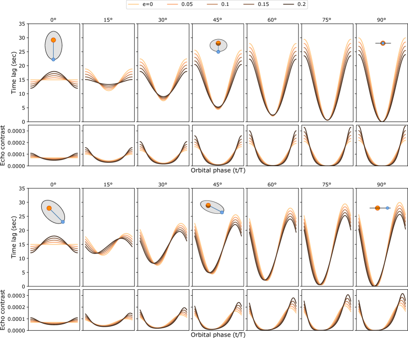
Figure 11: Jupiter-sized exoplanet at 0.03 au at eccentricities from 0-0.2 with argument of the periapsis oriented at 180^o (Top) and $135^{o}$ (Bottom) relative to Earth.

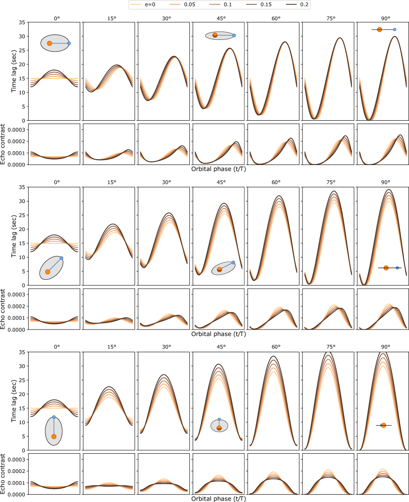
Figure 12: Jupiter-sized exoplanet at 0.03 au at eccentricities from 0-0.2 with argument of the periapsis oriented at 90^o (Top), $45^{o}$ (Center), and $0^{o}$ (Bottom) relative to Earth.

While this can be evaluated numerically for all orbits, we found that the probability of detecting echoes from an exoplanet in a circular orbit observed from an inclined view has a simple analytical form. To see this, we start with the lag as a function of time(Sparks et al., 2018):

$$\tau_{\text{echo}}(t)=\frac{a}{c}(1+\{\sin{2\pi t/T},\cos{2\pi t/T},0\}.\hat{e}_{\text{obs}})=\frac{a}{c}(1+\sin{2\pi t/T}\sin{\theta_{v}})$$ (B2)

This is readily inverted to give:

$$t(\tau_{\text{echo}})=\frac{T}{2\pi}\arcsin{\frac{c\tau_{\text{echo}}}{a}-1/\sin{\theta_{v}}}$$ (B3)

This form is only valid where arcsin is defined, which provides us with maximum and minimum lags of

$$\frac{a}{c}(1-\sin{\theta_{v}})<\tau_{\text{echo}}<\frac{a}{c}(1+\sin{\theta_{v}})$$ (B4)

This can be normalized to the arcsine cumulative density function, which has a variety of well-studied properties. One of the most important properties is that the modes of the distribution occur on the ends, and not near the mean (the arcsin probability density function is of the form $P(x)=1/\pi\sqrt{x(1-x)}$, which is infinite at $x=0,1$). Namely, there are two stationary points where the exoplanet would be more readily observed, shown in Figure 13. In the plot, we have also included the phase function weights.

Figure 13: Probability of an exoplanet in a circular orbit being visible to Earth for a given time lag as a function of inclination angle, weighted by flare view factor and assuming a Lambertian exoplanet. For face-on orientations, the probability function collapses to a single point at the center. For the transit case, the exoplanet is most visible when it is in superior conjunction.

Given that many of these lag structures will produce characteristic peaks, it is plausible to search for them without performing complete multi-dimensional searches. To evaluate the feasibility of performing lower-dimensional searches, we produced a simulation for a hot gas giant with of $R=2R_{J}$ around a star with numerous delta-like flares. Figure 14 shows data analysis results for 20 simulated periods for orbiting an active flare star. Fig. 14(a) shows the 1D correlation function, which has some promising peaks, but they are not sufficiently structured to be definitive. Fig. 14(b) shows how the flares and echo lags are distributed, illustrating why a 1D analysis is inadequate. Fig. 14(c) shows the ideal time lag and the associated distribution of lags as observed over a single period. Two prominent peaks are present with a higher density between them. A more realistic distribution is shown in Fig. 14(d), where the peaks have been weighted by the ideal exoplanet-star contrast. Indeed, this double-peak structure could be used as a matched filter search of the 1D lag function. Fig. 14(e) shows a period-folding analysis, showing higher signal strength in the predicted regions if the period is known precisely, but if the folding period is slightly off, say by 10% (Fig. 14(f)), the signal disappears. A comprehensive period-fold search is similar to the 4D approach described in §2. Alternatively, the workhorse of periodic searches is the Lomb-Scargle plot. The same dataset processed in this way produces Fig. 14(g), which shows a single significant peak. Examining only the period with this peak, Fig. 14(h), the structure of the two peaks is apparent and closely matches the distribution in (d), overlaid as the red dotted line. Again, the double-peak structure could be used as a matched filter search of a Lomb-Scargle plots.

Figure 14: Representative results for 1000 flares occurring over 20 periods for an exoplanet at 0.03 au, $R=2R_{J}$, orbital inclination of 15^o relative to Earth, eccentricity of 0.1, and argument of the periapsis at 90^o relative to Earth. (a) The simulated autocorrelation is not pristine due to the presence of multiple lags. (b) Analytical values for the echo lag as a function of orbit, as well as the random times that flares were sampled. (c) Phase-folded lags and their associated histogram (right) showing the most probable lags. (d) Exoplanet-star contrast as a function of orbit, used as a surrogate for echo contrast, and the impact on the lag detection histogram. (e) The orbital phase folded autocorrelation result when the exact phase is used. (f) The orbital phase folded autocorrelation result when the period is wrong by 10%. (g) Lomb Scargle plot for the detection showing two bright peaks associated with the orbital position. (h) Cross-section of the Lomb Scargle plot at the correct period, showing the same peaks in relatively similar structure as the predicted form from (c) and (d).

Appendix C An Echo Detection Algorithm

1. Produce a flare catalog. We identify flares in light curves using a trigger based on relative change in flux, and extract short segments of light curves that span individual flares and potential echoes. In the tests with simulated data that we perform here, each segment contains the integrated flux in $N_{t}\sim 10^{3}$ bins of width $\Delta t=0.1$ s, and covers a time $t_{\text{seg}}$ of 100 s, with the flare offset from the start of the segment by $\tau_{f}$, the typical flare decay time scale. We remove slowly varying modes in each segment by applying a high-pass filter,

   $$H(f)=1-\exp(-f^{2}/2\sigma^{2})$$ (C1)

   where $f$ is frequency, and $\sigma=2\pi/t_{\text{cut}}$, such that cut-off time $t_{\text{cut}}$ is three times $\tau_{f}$. The filtering is performed with fast Fourier transforms using the Python NumPy package(Oliphant, 2006).

2. Generate the discrete autocorrelation function, or “correlator,” of each light curve segment. The correlator for the $i^{\text{th}}$ light curve segment is

   $$\xi_{j}^{(i)}=\sum_{k=0}^{N_{t}-j}\tilde{F}^{(i)}_{k}\tilde{F}^{(i)}_{k+j}$$ (C2)

   where subscript $j$ designates the correlator’s lag, $\tau=k\Delta t$, $\tilde{F}^{(i)}_{k}$ is the filtered flux in a time bin at $t=k\Delta$ (relative to the start time of the light curve segment, $T_{i}$). To calculate the estimator in equation (C2), we use the Python NumPy correlate routine in “full” mode.(Oliphant, 2006) Then, to help with echo signal extraction, we flatten the correlator by subtracting a cubic fit to $(\log(t),\xi)$ on a domain with $t_{\text{cubic}}<t<t_{\text{seg}}$ (NumPy polyfit), where $t_{\text{cubic}}$ is chosen to be the typical flare decay time, $\tau_{f}$(Oliphant, 2006).

   We define a template function to identify echo candidates. Given that the shape of the echo in the correlation function should closely match the shape of the correlator at zero lag, we typically use a truncated, scaled version of the correlator itself.

3. Define a template function to identify echo candidates. Given that the shape of the echo in the correlation function should closely match the shape of the correlator at zero lag, we typically use a truncated, scaled version of the correlator itself,

   $${\Xi}^{(i)}_{j}={\xi}^{(i)}_{j}\ \ \ \text{($|j|\leq J_{0}$; zero otherwise)},$$ (C3)

   where $J_{0}$ correspond to a lag that is four time the value at which the average autocorrelation function drops to half of $\bar{\xi}_{0}$. This choice sets the half-width of the template to be approximately the flare decay time. We further set the average value of each template to zero to avoid coupling with the local correlator background near any potential echo location.

4. Determine a weight, $W_{i}$, for each of the $N_{f}$ correlators to provide a measure of the quality of each flare. The noise level is important, as is the orbital phase, but so is the flare light curve’s profile. For example, a flare that has all photons launched in a single time bin (a delta-function flare) might be high quality, while a brighter flare that is spread out over a long period of time, longer than the echo delay times of interest, could have lower quality. See Appendix D for a further discussion of weighting.

5. Set parameters needed to predict the echo delay for a planet in orbit about the flare star. As in the main text, we choose a 6D vector $\vec{P}$, with elements $M$, $a$, $e$, $M_{0}$, $\theta_{v}$ and $\phi_{v}$, where $M$ is the stellar mass, $a$ is the semimajor axis, $e$ is the orbital eccentricity, $M_{0}$ is the mean anomaly at some reference time $T_{0}$, while the last two parameters are spherical polar angles that determine the direction to the observer. We orient a coordinate system so that the planet lies in the $x$-$y$ plane ($\theta_{v}=\pi/2$) with periastron on the positive $x$-axis ($\theta_{v}=\pi/2$, $\phi_{v}=0$), and the planet’s orbital angular momentum vector defines the $z$-axis. Thus when a planet is observed face-on, $\theta_{v}=0$.

   For now we assume that all flares are centered on the host star, and discuss below how to relax this condition. Note that in general we may not always know the stellar mass accurately, and so may have to include the stellar mass $M$ as a sixth “orbital” parameter. Here, we assume $M$ is known.

   For a given set of orbital parameters $\vec{P}$, we shift and add the weighted correlators so that echo signals align and reinforce each other. The shift is calculated from the echo delay time of each flare,

   $$J_{e}=(\tau_{\text{echo}}-a_{f}/c)/\Delta t_{\text{bin}}$$ (C4)

   so that echo signals are centered in bin $\bar{J}_{e}$, corresponding to a lag of $a_{f}/c$, as if the planet were on a circular orbit at some fiducial semimajor axis $a_{f}$, observed face-on.

6. Build up the fingerprint of an echo. We start with a shifted, weighted correlator,

   $$S^{(i)}_{j}(\vec{P})\equiv W_{i}\,g_{j-J_{e}}\,\xi^{(i)}_{j-J_{e}},$$ (C5)

   where $W_{i}$ is the flare quality weight, and the function $g_{j-J_{e}}$ is unity so long as the lag shift does not move the peak of the correlator (originally at zero lag) close to the mean echo delay lag. In practice we prevent the shifting process from moving the flare peak to within twice the typical flare decay time of the mean echo delay time, though carefully chosen asymmetric templates may be able to provide echo correlation estimates. We note that the shortest echo lags typically correspond to orbital phases that are already unfavorable for detecting reflected light, so these data points are generally of lower detection value. Then

   $$\mathcal{S}(\vec{P})\equiv\frac{1}{W}\sum_{i=1}^{N_{f}}\sum_{j=-J_{0}}^{J_{0}}\Xi_{j}\,S_{\bar{J}_{e}-j}.$$ (C6)

   with $W$ the sum of weights. The quantity $\mathcal{S}(\vec{P})$ is an “echo correlator strength”, which serves as a measure of success in a search for echoes in a set of flares.

   Alternatively, with the same data, one form of a likelihood signature is (though it would typically be summed in log form):

   $$L(\vec{\xi}|\vec{P})=\prod_{i=1}^{N_{f}}\frac{1}{\sqrt{2\pi\sigma(W_{i}(j))^{2}}}\exp{\frac{-[\breve{\epsilon}^{(i)}_{j}(\vec{P})-(\Xi*S)(j)]^{2}}{2\sigma(W_{i}(j))^{2}}}$$ (C7)

   where $\breve{\epsilon}$ is the predicted echo correlator strength based on $\vec{P}$ for the observed flare, $j$ is the lag anticipated by the model at flare time $t$, and $(\Xi*S)(j)$ is the template convolution term from Eq. C6. To be strictly accurate, this requires making assumptions about the exoplanet radius and albedo; $R=R_{J}$, $p\sim 0.7$ is relatively robust first guess for the majority of echo-observable exoplanets. This form is also amenable to more detailed models, such as multi-planet systems, and is less likely to be contaminated by including a large number of microflares. The structure of $\sigma(W_{i}(j))^{2}$ is briefly discussed in Appx. D. This signature would then be maximized by a search routine.

7. Map the echo correlator strength over orbital elements, viewing angles, and (if necessary) stellar mass. We densely sample the 6D orbital parameter space on a grid, measuring $\cal{S}$ using equation (C5) at each grid point, $\vec{P}$. This procedure may involve as many as $10^{10}$ points, needed to map out $O(100)$ parameter values in typical ranges: $0.01~{}\text{au}<a<0.1~{}\text{au}$, $0<e<0.5$, $0^{\circ}<M<360^{\circ}$, $-90^{\circ}\theta_{v}<90^{\circ}$ and $0^{\circ}<\phi_{v}<180^{\circ}$). Note that there is a degeneracy in viewing angle values, since echo delays are symmetric to $(\theta_{v},\phi_{v})\rightarrow(-\theta_{v},\phi_{v}+\pi)$, so we only need to cover half the possible range of one or the other viewing angle. We find that we need the finest grid for the semimajor axis, and recommend a grid spacing $\Delta a$ that does not exceed

   $$\frac{\Delta a}{a}\sim 0.01\frac{T_{\text{period}}}{T_{\text{total}}}$$ (C8)

   where $T_{\text{period}}$ is the orbital period an $T_{\text{total}}$ is the total span of the observations. The reason is that a more accurate value of the period (hence $a$) is needed to line up the echo signals if the observations cover a larger number of orbits. This has the effect of requiring a smaller $\Delta a$ for longer observation times. Our simulations have only considered upwards of 10’s of periods, but for multi-year observations, such as those performed by Kepler, $\Delta a$ could become very small.

Appendix D Flare Weighting

This appendix is included as a discussion of potential weighting methods to increase the effectiveness of detection algorithms and is provided to motivate future work. To account for the fact that not all flares are equally useful, it can be helpful to weight the flares. The flare-background magnitude is the most obvious constraint. If the flare is 1% of the background signal, and the echo is $10^{4}$ times smaller, you will need more than a few measurements. Assuming Poisson noise, the average integrated noise for the quiescent background $Q$ over period $t_{int}$ is:

$$\langle N\rangle=\sqrt{Qt_{int}}$$ (D1)

For a flare with an integrated number of counts above the baseline of $f$, with length $t_{flare}$ the flare S/N is roughly:

$$s=\frac{f}{\sqrt{Qt_{flare}}}$$ (D2)

Therefore, a straightforward weight for the autocorrelation function of flare event $i$ is $s_{i}$. In this way, a small, brief flare can often have the same weight as a larger, long flare. However if the flare is bright and broad and not particularly useful, we look at the quality of the flare.

For a given orbit, the exoplanet will have a reduced probability of being viewed in certain positions, in accordance with its phase function. In simulating a candidate orbit, the predicted echo magnitude can be used as a weight in order to accentuate the highly visible parts of the orbit and to suppress orbital phases for which the echoes are fainter and prone to noise. Typically, a Lambertian approximation is used. Appendix B shows several examples of echo magnitudes, these would serve as the phase weight.

We can determine a quality for any given fluctuation from its time-bandwidth product properties that can be used as a weight. Using the time-frequency uncertainty relation ($\tau_{1/2}\Delta\omega\geq\frac{1}{2}$) and the threshold property found by localizing an echo to within half the travel time from the star to exoplanet of $\tau_{1/2}\gtrsim\tau_{\text{echo}}/2$, we can see the spectral bandwidth of a flare’s light curve must be at least

$$\Delta\omega\gtrsim\frac{1}{\tau_{\text{echo}}}$$ (D3)

Variability events with small spectral widths can be culled (a sine wave is useless, which has a delta-function spectral width). A good metric for the width of a pulse, $\Delta\omega$, is the inverse of the magnitude of the second moment of the Fourier transform of the flare. Thus, to weight the contribution to the autocorrelation function we can use $w_{i}=(\Delta\omega)_{i}$ for variability event $i$.

Not all fluctuations detected from Earth will occur on the same side of the star as the exoplanet, resulting in a systematic decorrelation if the data are blindly summed. For a face-on orbit, it is reasonable to expect about half of the localized fluctuation events (e.g. flares) to occur on the same side of the star as the exoplanet, and many that occur near the limb will be attenuated by the optical density of the star, depending on the depth of the fluctuation. For nearly edge-on systems, the odds become worse because the exoplanet’s phase function will be at its brightest at superior conjunction, which means it will primarily be illuminated by events that occur on the side of the star facing away from Earth. Then, at inferior conjunction, the lag and phase function will be zero, providing the worst possible detection conditions. Fortunately, transit and radial velocity detection methods work best under these conditions, so this regime is already accessible with existing techniques. Regardless, we must initially assign a weight, $w_{exo\_phase}$ of $\sim 50\%$ that there will be an echo, unless there are predictive factors like the position of active regions. To account for phase-dependent exoplanet visibility, one weight choice is the Lambertian phase function (Eq. B1), $w_{exo\_phase}=\phi(\alpha)$. In the case where an active region can be identified, a star-phase weight can be produced. In preliminary simulations, we found that using a limb-darkening model appears to be effective, though considerable work remains to make these models effective.

Typically, all of these weights will be combined into a composite weight, e.g.,

$$W_{i}=w_{i,freq}w_{i,mag}w_{i,\Delta\omega}w_{i,exo\_phase}$$ (D4)

or, for the maximum likelihood approach, they may be combined as:

$$\sigma(W_{i})^{2}=w_{i,freq}^{2}+w_{i,mag}^{2}+w_{i,\Delta\omega}^{2}+w_{i,exo\_phase}^{2}$$ (D5)

where the individual weights may require rescaling to have the appropriate relative balance.

References

- tes (2017) 2017, TESS Observatory Guide, v1.1 edn., TESS Science Support Center, NASA Goddard Space Flight Center, Greenbelt, MD
- Anglada-Escudé et al. (2016) Anglada-Escudé, G., Amado, P. J., Barnes, J., et al. 2016, Nature, 536, 437
- Argyle (1974) Argyle, E. 1974, Icarus, 21, 199
- Bolcar et al. (2017) Bolcar, M. R., Aloezos, S., Bly, V. T., et al. 2017, in Society of Photo-Optical Instrumentation Engineers (SPIE) Conference Series, Vol. 10398, Society of Photo-Optical Instrumentation Engineers (SPIE) Conference Series, 1039809
- Borucki et al. (2010) Borucki, W. J., Koch, D., Basri, G., et al. 2010, Science, 327, 977
- Bromley (1992) Bromley, B. C. 1992, PASP, 104, 1049
- Clark (2009) Clark, R. 2009, Master’s thesis, California State University, Fresno
- Crotts et al. (1989) Crotts, A. P. S., Kunkel, W. E., & McCarthy, P. J. 1989, ApJ, 347, L61
- Davenport et al. (2016) Davenport, J. R. A., Kipping, D. M., Sasselov, D., Matthews, J. M., & Cameron, C. 2016, ApJ, 829, L31
- Gaidos (1994) Gaidos, E. J. 1994, Icarus, 109, 382
- Giampapa et al. (1981) Giampapa, M. S., Worden, S. P., Schneeberger, T. J., & Cram, L. E. 1981, ApJ, 246, 502
- Gillon et al. (2017) Gillon, M., Triaud, A. H. M. J., Demory, B.-O., et al. 2017, Nature, 542, 456
- Han et al. (2014) Han, E., Wang, S. X., Wright, J. T., et al. 2014, PASP, 126, 827
- Hawley et al. (2014) Hawley, S. L., Davenport, J. R. A., Kowalski, A. F., et al. 2014, ApJ, 797, 121
- Hilton et al. (2010) Hilton, E. J., West, A. A., Hawley, S. L., & Kowalski, A. F. 2010, AJ, 140, 1402
- Horne et al. (1991) Horne, K., Welsh, W. F., & Peterson, B. M. 1991, ApJ, 367, L5
- Irwin et al. (2009) Irwin, J., Charbonneau, D., Nutzman, P., & Falco, E. 2009, in IAU Symposium, Vol. 253, Transiting Planets, ed. F. Pont, D. Sasselov, & M. J. Holman, 37–43
- Janson et al. (2013) Janson, M., Brandt, T. D., Moro-Martín, A., et al. 2013, ApJ, 773, 73
- Jones et al. (2001) Jones, E., Oliphant, T., Peterson, P., et al. 2001, SciPy: Open source scientific tools for Python
- Kennedy & Kenyon (2008a) Kennedy, G. M., & Kenyon, S. J. 2008a, ApJ, 682, 1264
- Kennedy & Kenyon (2008b) —. 2008b, ApJ, 673, 502
- Kennedy et al. (2006) Kennedy, G. M., Kenyon, S. J., & Bromley, B. C. 2006, ApJ, 650, L139
- Kenyon & Bromley (2014) Kenyon, S. J., & Bromley, B. C. 2014, ApJ, 780, 4
- Klocová et al. (2017) Klocová, T., Czesla, S., Khalafinejad, S., Wolter, U., & Schmitt, J. H. M. M. 2017, A&A, 607, A66
- Kowalski et al. (2016) Kowalski, A. F., Mathioudakis, M., Hawley, S. L., et al. 2016, ApJ, 820, 95
- Ledrew (2001) Ledrew, G. 2001, JRASC, 95, 32
- Lehner et al. (2012) Lehner, M. J., Wang, S.-Y., Alcock, C. A., et al. 2012, in Proc. SPIE, Vol. 8444, Ground-based and Airborne Telescopes IV, 84440D
- Lépine & Gaidos (2011) Lépine, S., & Gaidos, E. 2011, AJ, 142, 138
- Loyd & France (2014) Loyd, R. O. P., & France, K. 2014, ApJS, 211, 9
- Luger et al. (2017) Luger, R., Sestovic, M., Kruse, E., et al. 2017, Nature Astronomy, 1, 0129
- Mann et al. (2012) Mann, A. W., Gaidos, E., Lépine, S., & Hilton, E. J. 2012, ApJ, 753, 90
- Mann (2017) Mann, C. 2017, Stellar Echo Imaging of Exoplanets, Tech. rep., Nanohmics, available online: Posted 7 April, 2017
- Marois et al. (2008) Marois, C., Macintosh, B., Barman, T., et al. 2008, Science, 322, 1348
- Matloff & Fennelly (1976) Matloff, G. L., & Fennelly, A. J. 1976, Journal of the British Interplanetary Society, 29, 471
- Mayor et al. (2011) Mayor, M., Marmier, M., Lovis, C., et al. 2011, ArXiv e-prints, arXiv:1109.2497
- Meng et al. (2016) Meng, H. Y. A., Plavchan, P., Rieke, G. H., et al. 2016, The Astrophysical Journal, 823, 58
- Mennesson et al. (2016) Mennesson, B., Gaudi, S., Seager, S., et al. 2016, in Proc. SPIE, Vol. 9904, Space Telescopes and Instrumentation 2016: Optical, Infrared, and Millimeter Wave, 99040L
- Mullally et al. (2015) Mullally, F., Coughlin, J. L., Thompson, S. E., et al. 2015, ApJS, 217, 31
- Ogihara & Ida (2009) Ogihara, M., & Ida, S. 2009, ApJ, 699, 824
- Oliphant (2006) Oliphant, T. E. 2006, A guide to numpy
- Peterson & Horne (2004) Peterson, B. M., & Horne, K. 2004, Astronomische Nachrichten, 325, 248
- Pettersen et al. (1986) Pettersen, B. R., Panov, K. P., Ivanova, M. S., & Sandmann, W. H. 1986, A&AS, 66, 235
- Ragazzoni et al. (2016) Ragazzoni, R., Magrin, D., Rauer, H., et al. 2016, in Proc. SPIE, Vol. 9904, Space Telescopes and Instrumentation 2016: Optical, Infrared, and Millimeter Wave, 990428
- Rest et al. (2012) Rest, A., Sinnott, B., & Welch, D. L. 2012, PASA, 29, 466
- Russell (1916) Russell, H. N. 1916, ApJ, 43, 173
- Schmidt et al. (2014) Schmidt, S. J., Prieto, J. L., Stanek, K. Z., et al. 2014, ApJ, 781, L24
- Schmidt et al. (2016) Schmidt, S. J., Shappee, B. J., Gagné, J., et al. 2016, ApJ, 828, L22
- Silverman (1986) Silverman, B. W. 1986, Density estimation for statistics and data analysis (London: Chapman and Hall)
- Sparks et al. (2018) Sparks, W. B., White, R. L., Lupu, R. E., & Ford, H. C. 2018, The Astrophysical Journal, 854, 134
- Stelzer et al. (2013) Stelzer, B., Marino, A., Micela, G., López-Santiago, J., & Liefke, C. 2013, MNRAS, 431, 2063
- Sugerman (2003) Sugerman, B. E. K. 2003, AJ, 126, 1939
- Sumi et al. (2011) Sumi, T., Kamiya, K., Bennett, D. P., et al. 2011, Nature, 473, 349
- Traub & Oppenheimer (2010) Traub, W. A., & Oppenheimer, B. R. 2010, in Exoplanets, ed. S. Seager (Tucson: University of Arizona Press), 111–156
- Walkowicz et al. (2011) Walkowicz, L. M., Basri, G., Batalha, N., et al. 2011, AJ, 141, 50
- Welch (1967) Welch, P. D. 1967, IEEE Trans. Audio and Electroacoust., Volume AU-15, p. 70-73, 15, 70
- West et al. (2004) West, A. A., Hawley, S. L., Walkowicz, L. M., et al. 2004, AJ, 128, 426
- Yang et al. (2017) Yang, H., Liu, J., Gao, Q., et al. 2017, ApJ, 849, 36