Object reconstruction from multiplexed quantum ghost images using reduction technique

Abstract

We apply the measurement reduction technique to optimally reconstruct an object image from multiplexed ghost images (GI) while taking into account both GI correlations and object image sparsity. We show that one can reconstruct an image in that way even if the object is illuminated by a small photon number. We consider frequency GI multiplexing using coupled parametric processes. We revealed that the imaging condition depends on the type of parametric process, namely, whether down- or up-conversion is used. Influence of information about sparsity in discrete cosine transform and Haar transform bases on reconstruction quality is studied. In addition, we compared ordinary and ghost images when the detectors are additionally illuminated by noise photons in a computer experiment, which showed increased noise immunity of GI, especially with processing via the proposed technique.

Introduction

By now, to enhance human visual capability a vast high-tech base including highly sensitive, high-precision and high-speed cameras have been developed. Nevertheless, there still are objects whose direct optical observation is difficult. They are primarily halftone biological objects that are especially sensitive to illumination and thus, have to be investigated very delicately. Ghost imaging (GI) are one way of solving this problem, as it allows to obtain object images without direct observation of its spatial structure. For GI, correlated light beams are necessary. GI enables extraction of object information from spatial correlations between beams, one of which (in the object arm) interacts with the object, while the other one (in the reference arm) does not. In the object arm, a bucket detector is used, which provides only information about the total intensity of the transmitted radiation. The other beam does not interact with the object, but is detected by a CCD matrix, which permits measuring the spatial correlation function of intensity between two arms. The information about transparency or reflectivity distribution of the research object is extracted from photocount correlations in the object and reference arms [1], see also [2, 3, 4, 5, 6].

In this paper, we study application of multicomponent entangled quantum light states that let us produce several GI simultaneously (to multiplex GI) [7, 8, 9, 10] by using radiation with different frequencies in reference arms. Mutual correlations of multiplexed images are used as additional information to improve image processing in the presence of fluctuations. There are various ways of producing multi-frequency entangled light beams. The required states can be obtained, e. g., in consecutive coupled parametric interactions in nonlinear crystals located either outside [11, 12] or inside [13] an optical resonator, in nonlinear waveguide structures [14, 15] where modes are coupled through evanescent modes, in a spatially modulated pump beam [16]. The considered GI multiplexing employs four-frequency entangled quantum states formed through parametric decay of pump photons into two photons with different frequencies that are mixed in the same crystal with pump photons, which produces photons with sum frequencies [17, 18]. Quantum theory of this process has been systematically developed in recent years [19, 20, 21, 22]. Note that in [23, 24, 4] GI were multiplexed via multi-frequency noncoherent radiation sources to simultaneously produce several GI that are superimposed afterwards. Recently, polarization multiplexing has been used in several works on GI (see [25] and references there), in particular, to improve the reconstructed image quality.

The ghost image processing methods considered in the literature usually rely on regularization. The regularizing functional is a characteristic of image sparsity in a given basis [26, 27, 28, 29], and the minimized functional itself is the least squares one [27, 28, 29] or likelihood function [26]. Alternatively, a sparsity characteristic (e. g. the $L^{1}$ norm in a given basis) is minimized [30] under the constraint that measuring the image reconstructed in that way would give the results actually obtained. Since such functional is not connected the error of the interpretation result, the obtained estimate is, generally speaking, not the optimal one. Unlike [26], measurement reduction method, including its proposed version, does not require only Poisson photocount distribution, and unlike [26, 27, 30, 28, 29], image sparsity in any basis is not required.

Note the main differences between this article and publications [8, 9, 10], in which multiplexed GI processing using measurement reduction technique was employed as well. Firstly, in these works the situation was considered when the only information about transparency distribution available to the researcher was that its values belong to a unit interval. In this article, it is considered that the researcher also has information about transparency distribution sparsity in a given basis and wants to take advantage of it to improve estimation quality. Secondly, as this information enables reconstruction of acceptable quality even with a small number of photons illuminating the object, multiplexed ghost imaging with a small number of photons ($\sim 1\div 10$ photons per pixel) and processing of acquired images is modeled (see Sec. 3). Thirdly, the presented version of measurement reduction technique differs from the one used in [8, 9, 10] in that projection (to take into account the information about the object) minimizes Mahalanobis distance instead of Euclidean distance, see Eqn. (23) below. Finally, fourthly, in the studied multiplexed ghost imaging setup the object arm is lensless. This leads to imaging conditions depending on the type of parametric coupling of photon frequencies in the object arm and the reference arms.

The article structure is as follows. In section 1, we discuss GI multiplexing setup with lensless object arm and with lenses in reference arms. In section 2 the measurement reduction method is outlined. The information about the object that is available to the researcher and that is employed in reduction is summarized in subsection 2.1. In subsection 2.2, the algorithm of GI processing using reduction method that takes this information into account is described. Computer modeling results are given in section 3. Main results of the article are summarized in the conclusion.

1 Frequency multiplexing of quantum ghost images

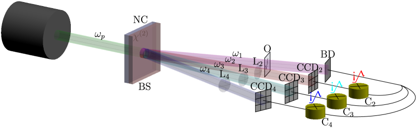
Figure 1: Multiplexed ghost imaging setup. NC is the nonlinear convertor; BS is the beam splitter; $\omega_{p}$ is pump frequency; $\omega_{1},\ldots,\omega_{4}$ are frequencies of produced entangled photons; $O$ is the object; BD is the bucket detector in the object arm; $L_{j}$ are lenses with focal lengths $f_{j}$; CCD_j are CCD in reference arms; C_j are intensity correlators, $j=2,3,4$

GI multiplexing setup is shown in fig. 1. The illumination is provided by coupled parametric processes that produce four-frequency entangled light fields. Pump radiation incident into the nonlinear convertor (nonlinear photon crystal) has frequency $\omega_{p}$. In the crystal, pump photons decay into two photons with related frequencies $\omega_{1}$ and $\omega_{2}$: $\omega_{p}=\omega_{1}+\omega_{2}$.

Four-frequency fields appear as a result of further conversion of a part of photons with frequencies $\omega_{1}$ and $\omega_{2}$ to photons with frequencies $\omega_{3}$ and $\omega_{4}$ in frequency-mixing processes:

$$\omega_{p}+\omega_{1} =\omega_{3},$$ (1)

$$\omega_{p}+\omega_{2} =\omega_{4}.$$

Efficient energy exchange between interacting light waves in these processes can be achieved in aperiodically nonlinear photon crystals, e. g. in $\mathrm{LiNbO}_{3}$, in the in quasi-phase matched regime, in which phase matching $\Delta k_{j}$ between interacting waves are compensated by the vectors of the inverse nonlinear lattice [17, 18]. Note that the considered process was recently realized via a setup with two nonlinear photon crystals in the work [31], where the spectrum of a photon pair at frequency above pump frequency was studied.

Let ghost images be obtained by means of the optical system setup shown in fig. 1, where a detector integrating radiation over the entire aperture is used in the object arm. It is assumed that the length of nonlinear photon crystal is chosen so that the transversal wave number amplification band of the nonlinear convertor substantially exceeds the width of wave spectrum of the object image. Details of four-frequency entangled state formation were considered in [7, 8, 9, 10].

In the setup of fig. 1 the object is illuminated by radiation with frequency $\omega_{1}$, which is detected by the bucket detector (BD) over the entire beam aperture, and therefore lacks spatial resolution. Radiation with other frequencies $\omega_{2},\omega_{3},\omega_{4}$ after their spatial separation enters reference arms with lenses in them. Focal lengths $f_{j}$ of lenses and their positions between the beam splitter (BS) and CCD cameras are chosen according to imaging conditions. These conditions depend on the type of relation to the frequency of object illumination. For frequencies $\omega_{2}$, $\omega_{4}$ the imaging condition has the form (cf. the analogous condition in [1] for equal frequencies)

$$\frac{1}{f_{j}}=\frac{1}{l_{j2}}+\frac{1}{l_{j1}+(\lambda_{1}/\lambda_{j})l_{11}},j=2,4,$$ (2)

while for frequency $\omega_{3}$ it reads (cf. the analogous condition in [32] for equal frequencies)

$$\frac{1}{f_{3}}=\frac{1}{l_{32}}+\frac{1}{l_{31}-(\lambda_{1}/\lambda_{3})l_{11}}.$$ (3)

In expressions (2), (3) the length $l_{11}$ is the distance from BS to the object, $l_{j1}$ is the distance from BS to the lens, $l_{j2}$ is the distance from the lens to the detector CCD_j, $\lambda_{j}$ is the length of the wave of corresponding frequency. The derivation of Eqns. (2), (3) is described below. They are a generalization of known ones to the case of different frequencies of radiation illuminating the object and radiation in reference arms.

The theory of formation of entangled quantum four-beam states in processes (1) was developed in [19, 20, 21]. Fourier components of Bose operators of field at nonlinear crystal output are represented in matrix form:

$$\hat{\mathbf{a}}(\mathbf{q},l)=Q(\mathbf{q},l){\hat{\mathbf{v}}}(\mathbf{q}),$$ (4)

Here $\hat{\mathbf{a}}$ and $\hat{\mathbf{v}}$ are columns of Bose operators at crystal output and input, respectively. They are of the form $\hat{\mathbf{a}}\operatorname{\overset{\text{def}}{=}}(\hat{a}_{1},\hat{a}_{2}^{\dagger},\hat{a}_{3},\hat{a}_{4}^{\dagger})^{T}$, where $T$ denotes transposition, $\hat{a}_{1}=\hat{a}_{1}(\mathbf{q},l)$, $\hat{a}_{2}^{\dagger}=\hat{a}_{2}^{\dagger}(-\mathbf{q},l)$, $\hat{a}_{3}=\hat{a}_{3}(\mathbf{q},l)$, $\hat{a}_{4}^{\dagger}=\hat{a}_{4}^{\dagger}(-\mathbf{q},l)$, $l$ is the length of nonlinear crystal. Operators in the column $\hat{\mathbf{v}}\operatorname{\overset{\text{def}}{=}}(\hat{v}_{1},\hat{v}_{2}^{\dagger},\hat{v}_{3},\hat{v}_{4}^{\dagger})^{T}$ refer to vacuum field state.

$Q$ is a $4\times 4$ matrix whose elements $Q_{mn}$ describe field conversion from frequency $\omega_{n}$ to frequency $\omega_{m}$. The form of the matrix $Q$ and its properties in the quasioptical approximation are given in [19]. The elements of $Q$ depend on crystal length, pump intensity and transversal wave number $\mathbf{q}$.

The opertor $\hat{a}_{j}(\mathbf{q},z)$ is the annihilation operator of plane mode photons with frequency $\omega_{j}$ and transversal wave vector $\mathbf{q}$:

$$\hat{a}_{j}(\mathbf{q},z)=\frac{1}{2\pi}\iint\limits_{-\infty}^{+\infty}\hat{A}_{j}(\boldsymbol{\rho},z)\exp(-i\mathbf{q}\boldsymbol{\rho})d\boldsymbol{\rho},$$ (5)

where $\hat{A}_{j}(\boldsymbol{\rho},z)$ is the slowly varying amplitude operator of the positive-frequency field

$$\hat{E}^{\dagger}_{j}(\mathbf{r},z,t)=\hat{A}_{j}(\mathbf{r},z,t)\exp(-i(\omega_{j}t-k_{j}z)),$$ (6)

$k_{j}$ is wave number, $z$ is the direction of propagation of interacting waves in the nonlinear crystal.

After BS, their amplitude operators are defined by the following relations

$$\hat{B}_{j}(\mathbf{r}_{j})=\int H_{j}(\mathbf{r}_{j},\boldsymbol{\rho}_{j}){\hat{A}}_{j}(\boldsymbol{\rho}_{j},l)d\boldsymbol{\rho}_{j},$$ (7)

in the detector plane, integration being over the light beam aperture. $H_{j}(\mathbf{r}_{j},\boldsymbol{\rho})$ is the medium response function for radiation propagation from the crystal to the detector in $j$-th arm. We assume for simplicity that beam splitting takes place directly at nonlinear crystal output. In other words, BS is considered to be thin.

For the object arm

$$H_{1}(\mathbf{r}_{1},\boldsymbol{\rho}_{1})=\int\limits_{-\infty}^{+\infty}H_{1}(\mathbf{r}_{1}-\boldsymbol{\rho}_{1}^{\prime};l_{12})T(\boldsymbol{\rho}_{1}^{\prime})H_{j}(\boldsymbol{\rho}_{1}^{\prime}-\boldsymbol{\rho}_{1};l_{11})d\boldsymbol{\rho}_{1}^{\prime}.$$ (8)

Here $T(\boldsymbol{\rho}_{1}^{\prime})$ is the object transmission coefficient, $H_{1}(\mathbf{r}-\boldsymbol{\rho};l_{1j})$ is the Green’s function

$$\int H_{1}(\mathbf{r}-\boldsymbol{\rho};l_{1j})=-i\frac{k_{1}}{2\pi l_{1j}}\exp\left(i\frac{k_{1}(\mathbf{r}-\boldsymbol{\rho})^{2}}{2l_{1j}}\right).$$ (9)

As noted above, $l_{11}$ is the distance between BS and the object and $l_{12}$ is the distance between the object and the bucket detector.

Response functions of reference arms containing thin lenses with focal length $f_{j}$ can be represented as (see [33, 34])

$$H_{j}(\mathbf{r}_{j},\boldsymbol{\rho}_{j})=-i\frac{k_{j}}{2\pi L_{j}}\exp\left(i\frac{k_{j}}{2L_{j}}\left[(\mathbf{r}_{j}-\boldsymbol{\rho}_{j})^{2}-(l_{j1}\mathbf{r}_{j}^{2}+l_{j2}\boldsymbol{\rho}_{j}^{2})/f_{j}\right]\right),$$ (10)

where

$$L_{j}=l_{j1}+l_{j2}-l_{j1}l_{j2}/f_{j}.$$

Intensity operators of the obtained beams are $\hat{I}_{j}(\mathbf{r}_{j})=\hat{B}^{\dagger}_{j}(\mathbf{r}_{j})\hat{B}_{j}(\mathbf{r}_{j})$. Mutual intensity correlation functions of the object arm and reference arms, taking into account Gaussian field statistics, are determined by the following formulas: for radiation with frequency $\omega_{3}$ the correlation function is

$$G_{13}(\mathbf{r}_{1},\mathbf{r}_{3})=\langle\hat{I}_{1}(\mathbf{r}_{1})\hat{I}_{3}(\mathbf{r}_{3})\rangle-\langle\hat{I}_{1}(\mathbf{r}_{1})\rangle\langle\hat{I}_{3}(\mathbf{r}_{3})\rangle=|\langle\hat{B}_{1}(\mathbf{r}_{1})\hat{B}_{3}^{\dagger}(\mathbf{r}_{3})\rangle|^{2},$$ (11)

while for radiation with frequencies $\omega_{2}$ or $\omega_{4}$ the correlation function is

$$G_{1j}(\mathbf{r}_{1},\mathbf{r}_{j})=\langle\hat{I}_{1}(\mathbf{r}_{1})\hat{I}_{j}(\mathbf{r}_{j})\rangle-\langle\hat{I}_{1}(\mathbf{r}_{1})\rangle\langle\hat{I}_{j}(\mathbf{r}_{j})\rangle=|\langle\hat{B}_{1}(\mathbf{r}_{1})\hat{B}_{j}(\mathbf{r}_{j})\rangle|^{2},j=2,4.$$ (12)

The difference in the definitions of the correlation functions under consideration is due to the type of parametric conversion and the initial vacuum fluctuations. As a consequence, only the vacuum operators in antinormal ordering contribute to correlations.

Under imaging conditions (2), (3) the expressions can be transformed to

$$G_{13}(\mathbf{r}_{1},\mathbf{r}_{3})=|\Gamma_{3}|^{2}\left|\frac{l_{31}(\lambda_{1}/\lambda_{3})l_{11}}{\lambda_{1}l_{12}l_{32}}T\left(-\alpha_{3}\mathbf{r}_{3}\right)\right|^{2},\alpha_{3}\operatorname{\overset{\text{def}}{=}}\frac{l_{31}-(\lambda_{1}/\lambda_{3})l_{11}}{l_{32}},$$ (13)

$$G_{1j}(\mathbf{r}_{1},\mathbf{r}_{j})=|\Gamma_{j}|^{2}\left|\frac{l_{j1}(\lambda_{1}/\lambda_{j})l_{11}}{\lambda_{1}l_{12}l_{j2}}T\left(-\alpha_{j}\mathbf{r}_{j}\right)\right|^{2},\alpha_{j}\operatorname{\overset{\text{def}}{=}}\frac{l_{j1}+(\lambda_{1}/\lambda_{j})l_{11}}{l_{j2}}.$$ (14)

These formulas are derived under the assumption that at the nonlinear crystal output, mutual correlation functions of the radiation

$$\Gamma_{1j}(\boldsymbol{\rho}_{1}-\boldsymbol{\rho}_{j})=\langle\hat{A}_{1}(\boldsymbol{\rho}_{1},l)\hat{A}_{j}(\boldsymbol{\rho}_{j},l)\rangle=(2\pi)^{-1}\int Q_{11j}(\mathbf{q})\exp(i\mathbf{q}(\boldsymbol{\rho}_{1}-\boldsymbol{\rho}_{j}))d\mathbf{q},j=2,4,$$

$$\Gamma_{13}(\boldsymbol{\rho}_{1}-\boldsymbol{\rho}_{3})=\langle\hat{A}_{1}(\boldsymbol{\rho}_{1},l)\hat{A}_{j}^{\dagger}(\boldsymbol{\rho}_{3},l)\rangle=(2\pi)^{-1}\int Q_{113}(\mathbf{q})\exp(-i\mathbf{q}(\boldsymbol{\rho}_{1}-\boldsymbol{\rho}_{3}))d\mathbf{q},$$

where $Q_{11n}(\mathbf{q})\operatorname{\overset{\text{def}}{=}}Q_{11}(\mathbf{q})Q_{n1}^{*}(\mathbf{q})+Q_{13}(\mathbf{q})Q_{n3}^{*}(\mathbf{q})$, $n=1,2,3$, are substituted by $\delta$-functions

$$\Gamma_{1n}(\boldsymbol{\rho}_{1}-\boldsymbol{\rho}_{n})=\Gamma_{n}\delta(\boldsymbol{\rho}_{1}-\boldsymbol{\rho}_{n}),\Gamma_{n}=\int\Gamma_{1n}(\boldsymbol{\rho})d\boldsymbol{\rho}.$$

These substitutions are valid if the radiation correlation radius is much smaller than a characteristic spatial scale of object image change.

The expressions (13), (14) coincide, up to a factor before the image transmission coefficient, with the expression obtained for another experimental setup [9, 10]. In [9, 10] ghost image correlations determined by fourth-order intensity correlations (eight-order field ones) were studied as well. Obviously, in the setup under consideration they will be the same as in [9, 10]. After integration over the area $s$ of the beam in the object arm (over $d\mathbf{r}_{1}$) intensity correlation functions of the second order, in accordance with (13), (14), becomes

$$G_{j}(\mathbf{r}_{j})\sim s\left|T(-\alpha_{j}\mathbf{r}_{j})\right|^{2},$$ (15)

while the GI correlation function determined by eighth-order field correlation function becomes

$$K_{ij}^{\textnormal{GI}}(\mathbf{r}_{i},\mathbf{r}_{j})\sim s^{2}|T(-\alpha_{i}\mathbf{r}_{i})|^{2}|T(-\alpha_{j}\mathbf{r}_{j})|^{2}.$$ (16)

Naturally, the coefficients $\alpha_{2},\alpha_{3},\alpha_{4}$ can be made equal by choice of setup parameters. In addition, in the following formulas (18) and (19) the factors dependent on the measurement unit choice will be omitted for brevity.

As mentioned above, the correlation functions derived above provide the information about the measuring (image acquisition) process that is used in the measurement reduction technique along with the information about the object. The following section focuses on the measurement reduction technique itself and the information about the object. Not all of the information mentioned above is equal in importance: only the correlation function (15) and finiteness of $L^{2}$ norm of the correlation function (16) for all $i,j=2,3,4$ are strictly necessary for image reconstruction. Nevertheless, additional information about both the measuring process (in our case, the form of correlation function (16)) and the object (sparsity of its transparency distribution) can vastly improve reconstruction quality, as it will be shown below.

2 Processing of acquired images

The output of $i$-th correlator, denoted as $\xi^{(i)}(\mathbf{r})$, can be considered as the impact of a measuring transducer (MT) on the input signal $f(\mathbf{r})\sim|T(-\mathbf{r})|^{2}$. Here and below, unlike the previous section, $f$ denotes the vector describing the object transparency distribution instead of focal length. We assume for simplicity that $\alpha_{2}=\alpha_{3}=\alpha_{4}=1$.

We will consider piecewise constant images, i. e. transparency is constant within each pixel. Areas of constant transparency and constant brightness corresponding to pixels are considered to be ordered in an arbitrary but fixed way. Due to that it is sufficient for us to consider a finite number of values of $\mathbf{r}$. Thus, $f$ as the vector of transparencies is an element of finite-dimensional Euclidean space $\mathcal{F}$.

An image processing algorithm ought to provide the most accurate estimate of the feature of the original image $f$ that is of interest to the researcher based on obtained data $\xi$, which consists of acquired ghost images $\xi^{(i)}(\mathbf{r})$, $i=2,3,4$. Measurement reduction method allows to obtain such an estimate. Let us formulate the measurement model as

$$\xi=\mathbf{A}f+\nu,$$ (17)

where $f$ is an priori unknown vector that describes the transparency distribution of the object, $\nu$ is measurement error with zero expectation, $\operatorname{\mathbb{E}}\nu=0$, which means absence of systematic measurement error, and covariance matrix $\mathbf{\Sigma}_{\nu}=\operatorname{\mathbb{E}}\nu\nu^{*}$. The matrix $\mathbf{A}$ describes ghost imaging and GI acquisition: the matrix element $\mathbf{A}_{ij}$ is equal to the mean output of $i$-th detector for unit transparency of $j$-th element of the object and zero transparency of other object elements (i. e. whose indices differ from $j$). The dimension of vector $f$ is the number of pixels in the object image, while the dimension of $\xi$ is the number of pixels in all CCD. The condition of systematic measurement error absense $\operatorname{\mathbb{E}}\nu=0$ means, in particular, that the expectation of the component of measurement results caused by detector dark noises is subtracted from the measurement results, similar to [35].

Matrices $\mathbf{A}$ and $\mathbf{\Sigma}_{\nu}$ are related to the correlation functions considered above. The measuring setup employs correlators that measure correlations between the object arm and other arms. Therefore, the matrix $\mathbf{A}$, which models the impact of MT on the image, is a block matrix and consists of three blocks describing correlator outputs, i. e. correlations between the object arm and reference arms:

$$\mathbf{A}=\begin{pmatrix}\mathbf{B}_{2}\mathbf{C}_{2}\\ \mathbf{B}_{3}\mathbf{C}_{3}\\ \mathbf{B}_{4}\mathbf{C}_{4}\end{pmatrix}.$$ (18)

Under the conditions used to derive the intensity correlation functions (15) and (16) the matrices $\mathbf{C}_{2}$–$\mathbf{C}_{4}$ are identity ones multiplied by pixel size and the factor before $|T(\mathbf{r}_{i})|^{2}$ in expression (15) for the correlation function $G_{j}$. The matrices $\mathbf{B}_{2}$–$\mathbf{B}_{4}$ model the detectors. Specifically, the matrix element $(\mathbf{B}_{i})_{pk}$ is equal to the output of the detector in $i$-th arm at $p$-th position for unit brightness of $k$-th pixel and zero brightness of other pixels.

Noise covariance matrix has block form as well:

$$\mathbf{\Sigma}_{\nu}=\begin{pmatrix}\mathbf{B}_{2}\mathbf{\Sigma}_{22}(f)\mathbf{B}_{2}^{*}&\mathbf{B}_{2}\mathbf{\Sigma}_{23}(f)\mathbf{B}_{3}^{*}&\mathbf{B}_{2}\mathbf{\Sigma}_{24}(f)\mathbf{B}_{4}^{*}\\ \mathbf{B}_{3}\mathbf{\Sigma}_{32}(f)\mathbf{B}_{2}^{*}&\mathbf{B}_{3}\mathbf{\Sigma}_{33}(f)\mathbf{B}_{3}^{*}&\mathbf{B}_{3}\mathbf{\Sigma}_{34}(f)\mathbf{B}_{4}^{*}\\ \mathbf{B}_{4}\mathbf{\Sigma}_{42}(f)\mathbf{B}_{2}^{*}&\mathbf{B}_{4}\mathbf{\Sigma}_{43}(f)\mathbf{B}_{3}^{*}&\mathbf{B}_{4}\mathbf{\Sigma}_{44}(f)\mathbf{B}_{4}^{*}\end{pmatrix}+\mathbf{\Sigma}_{\nu^{\prime}}.$$ (19)

Here the element with indices $k$, $k^{\prime}$ of the block $\mathbf{\Sigma}_{ij}$ is equal to the integral of $K_{ij}^{\textnormal{GI}}$ (16) over the values of $\mathbf{r}_{i}$ belonging to $k$-th pixel and over the values of $\mathbf{r}_{j}$ belonging to $k^{\prime}$-th pixel, for the same pixel ordering as in the matrix $\mathbf{A}$. Hence, the dependence of (19) on $f$ is caused by the dependence on $|T(\cdot)|^{2}$ of the correlation function $K_{ij}^{\textnormal{GI}}$ (16). The term $\mathbf{\Sigma}_{\nu^{\prime}}$ is the covariance matrix of the noise component $\nu^{\prime}$ that is unrelated to ghost imaging, e. g. thermal noise in circuits and digitization error. Most of the noise arising before the correlators is suppressed by them if noise in object and reference arms is independent, but this does not apply to noise arising after the correlators. Besides, due to finite coincidence circuit match time some of noise photons contribute to the noise as well, see discussion of fig. 4 below.

It should be noted that the algorithm proposed below can be applied for an image multiplexing method that differs from the one considered in section 1 if the measurement model has the form (17). Specifically the expectation of measurement result has to be the product of a matrix $\mathbf{A}$ and the transparency distribution vector of the measured object, and the error has to be able to be considered additive. For that, the fourth-order intensity correlation function (an analog of (15)) has to linearly depend on the transparency distribution, and the eighth-order intensity correlation function (an analog of (16)) has to “sufficiently weakly” depend on the transparency distribution so that an unknown covariance matrix could be estimated using measurement results. If, in addition to that, photon detections in reference arms are conditionally independent under fixed output of the bucket detector in the object arm (output of a detector in a reference arm does not affect output of detectors in other reference arms), then what was said about the form of matrices $\mathbf{A}$ and $\mathbf{\Sigma}_{\nu}$ remains valid.

The estimation problem consists of reconstruction of the most accurate estimate of the signal $\mathbf{U}f$ from the measurement result $\xi$, where the matrix $\mathbf{U}$ describes a measuring device that is ideal (for the researcher). We consider the case when the researcher is interested in reconstruction of the object image itself, and imaging does not distort the object, therefore, $\mathbf{U}=I$.

Since measurement results linearly depend on $f$, to solve the estimation problem we can use the model $[\mathbf{A},\mathbf{\Sigma}_{\nu},\mathbf{U}]$ described in [36], see also [37, 38, 39, 40]. If the estimation process is described by a linear operator $R$ ($R\xi$ is the result of processing the measurement $\xi$), the corresponding mean squared error (MSE) in the worst case of $f$, $h(R,\mathbf{U})=\sup\limits_{f\in\mathcal{F}}\operatorname{\mathbb{E}}\lVert R\xi-\mathbf{U}f\rVert^{2}$, as shown in [36], is minimal for $R$ that is equal to the linear unbiased reduction operator

$$R_{*}\operatorname{\overset{\text{def}}{=}}\mathbf{U}(\mathbf{A}^{*}\mathbf{\Sigma}_{\nu}^{-1}\mathbf{A})^{-}\mathbf{A}^{*}\mathbf{\Sigma}_{\nu}^{-1},$$ (20)

where ^- denotes pseudoinverse. $h(R_{*},\mathbf{U})=\operatorname{tr}\mathbf{U}(\mathbf{A}^{*}\mathbf{\Sigma}_{\nu}^{-1}\mathbf{A})^{-1}\mathbf{U}^{*}$, and the covariance matrix of the linear reduction estimate $R_{*}\xi$ is

$$\mathbf{\Sigma}_{R_{*}\xi}=\mathbf{U}(\mathbf{A}^{*}\mathbf{\Sigma}_{\nu}^{-1}\mathbf{A})^{-1}\mathbf{U}^{*}.$$ (21)

Estimation is possible (MSE is finite) if the condition $\mathbf{U}(I-\mathbf{A}^{-}\mathbf{A})=0$ holds, where, as noted above, $\mathbf{A}$ characterizes the real measuring device, while $\mathbf{U}$ characterizes an ideal one with the point spread function required by the researcher, and, therefore, any desired resolution, if this condition if fulfilled. Note that, unlike fluorescence-based superresolution techniques, see e. g. [41], the proposed technique does not require attaching fluorescent molecules to the object. However, as a rule, the better the desired resolution of the ideal measuring device compared to the resolution of the real one, the larger MSE of the obtained estimate. By choosing $\mathbf{U}$ one can select an acceptable (to him) compromise between obtained resolution and noise magnitude. In the case under consideration, as seen from (18), diagonal elements of each block (which, up to a nonzero factor, are equal to the factor before $|T(-\mathbf{r}_{j})|^{2}$ in the expression for correlation function $G_{j}$) are nonzero. Therefore, each block $\mathbf{A}_{j}$ is non-degenerate, so for non-degenerate $\mathbf{B}_{j}$ the reduction error takes only finite values. For a different multiplexing method and thus, different form of the matrix $\mathbf{A}$ this is generally not so.

The measurement reduction technique for the case when it is known that the value $u$ of the feature of interest is an arbitrary element not of the entire $\mathcal{U}$ but of its convex closed subset $\mathcal{U}_{\textnormal{pr}}$ was considered in [40, 42]. The estimate refinement which takes advantage of this information is determined by solving the equation

$$\hat{u}=\Pi_{\mathbf{\Sigma}_{R_{*}\xi}}\left(\tilde{R}_{\mathbf{\Sigma}_{R_{*}\xi}}\left(\xi^{T},\hat{u}^{T}\right)^{T}\right)$$ (22)

for $\hat{u}$, where $\tilde{R}_{\mathbf{\Sigma}_{R_{*}\xi}}$ is the measurement reduction operator for a MT $\left(\mathbf{A}^{T},\mathbf{U}^{T}\right)^{T}$ and noise with covariance matrix $\begin{pmatrix}\mathbf{\Sigma}_{\nu}&0\\ 0&\mathbf{\Sigma}_{R_{*}\xi}\end{pmatrix}$, and the operator

$$\Pi_{\mathbf{\Sigma}_{R_{*}\xi}}(u)\operatorname{\overset{\text{def}}{=}}\operatorname*{argmin}\limits_{v\in\mathcal{U}_{\textnormal{pr}}}(v-u,{\mathbf{\Sigma}_{R_{*}\xi}}^{-1}(v-u))$$ (23)

describes projection onto $\mathcal{U}_{\textnormal{pr}}$ by minimizing Mahalanobis distance $\lVert\mathbf{\Sigma}_{R_{*}\xi}^{-1/2}\cdot\rVert$ that is related to covariance matrix $\mathbf{\Sigma}_{R_{*}\xi}$ (21) of error of the linear reduction estimate $R_{*}\xi$. Note that the version of reduction technique proposed in [10] and in [40] for similar information used minimization of the “ordinary” Euclidean distance instead of Mahalanobis distance. In [42], the advantages of minimizing Mahalanobis distance instead of Euclidean distance during projection are shown. In that case the covariance matrix (21) of linear reduction estimate error is an upper bound on the covariance matrix of the obtained estimate.

2.1 Representation of the object information that is available to the researcher

It is obvious that a priori $|T(-\mathbf{r}_{j})|^{2}\in[0,1]$, hence $f\in[0,1]^{\dim\mathcal{F}}$, $\mathbf{U}f\in[0,1]^{\dim\mathcal{F}}$.

It is assumed that the transparency distribution of the object is not “entirely” arbitrary: transparencies of neighboring pixels usually do not differ much, so the image is sparse (many of its components are zero) in a given (a priori known) basis, similarly to compressed sensing ghost imaging [26, 29, 35].

The researcher also knows the matrix $\mathbf{A}$ (18) that describes image acquisition conditions and, up to the vector $f$, the matrix $\mathbf{\Sigma}_{\nu}$ (19) that describes measurement errors. Note that the worst case of $f$ is realized if all pixels are equally transparent. For a different multiplexing method one considers the worst case in the sense of reduction MSE of the object in step 1 of the algorithm below.

2.2 Reduction algorithm

The proposed algorithm of multiplexed GI processing using measurement reduction technique that is based on the indicated prior information has the following form.

1. Calculation of linear unbiased reduction estimate $R_{*}\xi$ (20) based on the acquired GI, assuming for calculation of covariance matrix (19) that all pixels have the same brightness.

2. Refinement of the estimate $R_{*}\xi$ using the information $\mathcal{U}_{\textnormal{pr}}=[0,1]^{\dim\mathcal{F}}$ by the method (22) by fixed-point iteration, i. e. by consecutive application of the mapping (22) with $\Pi_{\mathbf{\Sigma}_{R_{*}\xi}}(R_{*}\xi)$ as the initial approximation. We denote the obtained estimate by $\hat{u}$.

3. Application of the sparsity-inducing transformation $T$ to $\hat{u}$. “Sparsity-inducing” means that the transformation is chosen by the researcher so that, in his opinion, the transform of the true transparency distribution of the object is sparse.

4. Calculation of maximal (in the worst case of $f$) variances $\sigma_{T\hat{u}}^{2}=(\sigma_{(T\hat{u})_{1}}^{2},\dots,\sigma_{(T\hat{u})_{\dim\mathcal{F}}}^{2})$ of the components of $T\hat{u}$, i. e. the diagonal matrix elements of $T\mathbf{\Sigma}_{R_{*}\xi}T^{*}$, and calculation of $T\hat{u}_{\textnormal{thr}}$: $(T\hat{u}_{\textnormal{thr}})_{i}\operatorname{\overset{\text{def}}{=}}0$ if $|(T\hat{u})_{i}|<\lambda\sigma_{(T\hat{u})_{i}}$, otherwise $(T\hat{u}_{\textnormal{thr}})_{i}\operatorname{\overset{\text{def}}{=}}(T\hat{u})_{i}$.

5. Inverse transformation $T^{-1}$ of $T\hat{u}_{\textnormal{thr}}$ (if $T$ is a unitary transformation, then $T^{-1}=T^{*}$), i. e. calculation of $\hat{u}_{\textnormal{thr}}\operatorname{\overset{\text{def}}{=}}T^{-1}T\hat{u}_{\textnormal{thr}}$.

6. Calculation of the projection $\Pi_{\mathbf{\Sigma}_{R_{*}\xi}}(\hat{u}_{\textnormal{thr}})$ that is considered to be the result of processing obtained ghost images.

The value of $\lambda\geq 0$ is a parameter of the algorithm. It reflects a compromise between noise suppression (the larger the value of $\lambda$, the greater the noise suppression) and distortion of images whose components are close to $0$. Step 4 can be considered as testing a statistical hypothesis, according to which $(T\mathbf{U}f)_{i}=0$ (for the alternative hypothesis that $(T\mathbf{U}f)_{i}\neq 0$) for all $i$. In this paper to do that we employ in step 4 a simple criterion based on Chebyshev’s inequality: if $(T\mathbf{U}f)_{i}=0$, then $\Pr\left(|(T\hat{u})_{i}|\geq\lambda\sigma_{(T\hat{u})_{i}}\right)\leq\lambda^{-2}$. Due to that one can suppose that image distortion is insignificant for, at least, $\lambda\leq 1$, as such distortion would be indistinguishable from the noise. Step 4 can be also interpreted as replacement of the original matrix $\mathbf{U}$ with one whose kernel contains the estimate components after the specified transform that are affected by the noise the most.

In [10] the matrix $\mathbf{U}$ was chosen to suppress the noise more, even at the cost of potential image distortion (e. g. worse resolution), by discarding the most noisy components of the image. Unlike [8, 9, 10], here we consider components of the image in a basis specified by the researcher instead of the eigenbasis [36, ch. 8] of the measurement interpretation model, i. e. a basis determined by error properties. In this article the basis is defined by the transformation whose result for the true transparency distribution is sparse, but the discarded components are determined, as in [10], by the measurement error. Thus, to improve estimation quality not only information about the noise is used, but also information about the object, namely, the properties of the transparency distribution (in the opinion of the researcher) and its features of interest.

3 Computer modeling results

The results of processing of obtained GI as described above are shown in fig. 2 and 3. The detectors in reference arms are identical ones that are three times as large as an element of the object image. Therefore, image processing via measurement reduction increases resolution in addition to noise suppression. Modeling was carried out for the same parameters of the optical setup as in [10]: beam wave numbers $k_{1}=6\cdot 10^{4}\leavevmode\nobreak\ \textnormal{cm}^{-1}$, $k_{3}=1.7\cdot 10^{5}\leavevmode\nobreak\ \textnormal{cm}^{-1}$, crystal parameter $\beta=10\leavevmode\nobreak\ \textnormal{cm}^{-1}$, crystal parameter $\xi=\gamma/\beta=0.4$.

a Transparency distribution of the object

b GI

c Reduction result without sparsity information

d DCT, $\lambda=1.25$

e DCT, $\lambda=2.0$

f Haar transform, $\lambda=1.0$

g Haar transform, $\lambda=2.0$

h Haar transform, $\lambda=3.0$

Figure 2: GI processing by the developed algorithm: (2a) is the object, $64$x$64$ pixels, that is illuminated by $1$ photon per pixel on average, (2b) are its acquired GI, and (2c–2h) are image reduction results: (2c) is the result of reduction without sparsity information, (2d–2h) are results of reduction using information about sparsity in (2d–2e) discrete cosine transform (DCT), (2f–2h) Haar transform bases. The parameter $\lambda\geq 0$ of the image processing algorithm reflects a compromise between noise suppression (the larger the value of $\lambda$, the greater the noise suppression) and distortion of images whose components are close to $0$

a Transparency distribution of the object

b GI

c DCT, $\lambda=1.0$

d DCT, $\lambda=1.5$

e DCT, $\lambda=2.0$

f Haar transform, $\lambda=1.0$

g Haar transform, $\lambda=1.5$

h Haar transform, $\lambda=2.0$

Figure 3: GI processing by the developed algorithm: (3a) is the object, $64$x$64$ pixels, that is illuminated by $10$ photons per pixel on average, (3b) are its acquired GI, and (3c–3h) are results of reduction using information about sparsity in (3c–3e) discrete cosine transform (DCT), (3f–3h) Haar transform bases

One can see that additional information about sparsity allows to suppress noise more but its impact on obtained resolution is weak. As expected, for $0\leq\lambda\leq 1$ the distortion is undistinguishable from the noise. Further increase of $\lambda$ leads to better noise suppression (cf., e. g., fig. 2c and 2d, 3c and 3d), but also leads to more severe distortions caused by discarding “significant” image components as well (cf., e. g., fig. 2e and 3e). For large $\lambda$, their influence outweighs the improvement of image quality due to noise suppression, as small-scale image details are suppressed as well. Therefore, the optimal value of $\lambda$ depends on one’s intentions: one should choose the maximal value of $\lambda$ that preserves the details of interest. To do that, one can model acquisition of a test image that contains the required details and choose the largest value of $\lambda$ that preserves them, or specify the value of $\lambda$ after comparing reduction results for different $\lambda$. In the case of an object with sharp transparency changes (fig. 2) the additional information allowed to suppress false signal where the object is opaque, but only for Haar transform (discrete cosine transform (DCT) causes increased false signal in that region).

The transform whose result for the transparency distribution of the object is sparse that is usually employed in ghost image processing by the means of compressed sensing is DCT [35, 26, 29]. In [43], several transforms (identity transform, discrete wavelet transform and DCT) were reviewed and the advantages of DCT were shown. However, it seems that Haar transform may be preferable in the case of a transparency distribution that contains areas of weakly changing transparency with sharp borders if these areas are large compared to the resolution of the ideal measuring transducer and the location of the borders is important to the researcher. This assumption is verified by fig. 2f–2g, where one can see that Haar transform in this case, as opposed to fig. 3, allows larger $\lambda$ values without causing significant distortions, cf., e. g., fig. 2e and 2g, where the usage of DCT causes blurring of transversal slit borders for the same value of $\lambda$.

a Ordinary image

b Result of reduction of the ordinary image without sparsity information

c DCT, $\lambda=1.25$

d GI + $1$ noise photons

e DCT, $\lambda=1.25$

f GI + $5$ noise photons

g DCT, $\lambda=1.25$

Figure 4: Ordinary and ghost image processing by the developed algorithm. (4a) is the ordinary image of the object from fig. 3a obtained by illuminating it by $10$ photons per pixel on average and $10$ noise photons, and (4b) and (4c) are the results of its reduction (4c) without sparsity information and (4c) with information about sparsity in DCT base. (4d, 4f) are GI impacted by $1$ and $5$ noise photons, respectively. (4e, 4g) are the results of their reduction with information about sparsity in DCT base

In fig. 4 GI are compared with ordinary images if noise photons, which do not carry information about the object, but increase noise, are present. Due to employing correlations to acquire GI, noise photons usually do not affect detected images, as this requires simultaneous detection of a noise photon by one detector and another photon by a different detector. Nevertheless, due to finite coincidence windows and finite widths of the light filters before the detectors the noise photons do increase the measurement errors. One can see that due to suppression of most noise photons the quality of the reconstructed image is better than the quality of the image reconstructed using the ordinary image for the same number of noise photons. Moreover, when taking advantage of sparsity information ghost imaging allows to exploit larger $\lambda$ values and thus, to suppress the noise more (cf., e. g., fig. 4c and 4g). In this case multiplexing provides the means for further noise suppression if noise photons in different arms are detected independently.

Therefore, formalization the researcher’s information about sparsity of the object transparency distribution by Haar transform is preferable if it has areas of weakly changing transparency with sharp borders that are large compared to the resolution of the ideal measuring transducer and the location of the borders is important to the researcher. DCT is preferable if the transparency distribution has small transparency changes that have to be present in the estimate, e. g. biological objects without high-contrast borders. The values of $\lambda\sim 1\div 1.5$ are optimal if small-scale details are present and are of interest. Otherwise, larger $\lambda$ values are advisable.

Conclusion

The actual problem of increasing noise immunity is exacerbated by photon transmission and detecton in photocounting mode due to higher information content of each photon or its absense. Multiplexing of ghost images allows to reduce the noise level, since it increases the amount of transmitted information, enabling improvement the quality of processing of acquired data. In this case the additional information available to the researcher about the measurement process and about the object allows further noise suppression under the same detection conditions. Alternatively, one can make the detection conditions worse (e. g. to reduce the number of photons) while preserving the same estimation quality. The additional information about the measuring process in this work is the correlation functions of multiplexed ghost images. The additional information about the object is the information that the object transparency distribution is not arbitrary, namely, transparencies of neighboring pixels, as a rule, differ only slightly. This information is formalized as sparsity of the result of a given transform (e. g. DCT) of the transparency distribution, similar to compressed sensing.

In compressed sensing, as a rule, the measurement error is modeled as an arbitrary vector with bounded norm. Instead, in the proposed method it is modeled as a random vector, and selection of the estimate components which are considered to be zero is based on the statistical properties of the estimate components, namely, their variances. The use of covariances of the estimate components in addition to their variances is a subject of further research.

We consider that computer modeling based on the developed algorithm showed high efficiency of the developed reduction technique of ghost image processing in the sense of improvement of both their quality and their noise immunity. It is of interest to apply this technique in the field of quantum image processing for parametric amplification of images and frequency conversion.

The authors are grateful for help to T. Yu. Lisovskaya. This work was supported by RFBR grant 18-01-00598-A.

This is a pre-print of an article published in Quantum Information Processing. The final authenticated version is available online at: https://doi.org/10.1007/s11128-019-2193-x

References

- [1] A. V. Belinskii and D. N. Klyshko. Two-photon optics: diffraction, holography, and transformation of two-dimensional signals. Journal of Experimental and Theoretical Physics, 78(3):259–262, 1994.
- [2] A. Gatti, E. Brambilla, M. Bache, and L. A. Lugiato. Correlated imaging, quantum and classical. Physical Review A, 70(1):013802, 2004.
- [3] A. Gatti, E. Brambilla, M. Bache, and L. A. Lugiato. Ghost imaging. In M. I. Kolobov, editor, Quantum Imaging, chapter 5, pages 79–111. Springer, 2007.
- [4] K. W. C. Chan, M. N. O’Sullivan, and R. W. Boyd. High-order thermal ghost imaging. Optics Letters, 34(21):3343–3345, 2009.
- [5] B. I. Erkman and J. H. Shapiro. Ghost imaging: from quantum to classical to computational. Advances in Optics and Photonics, 2(4):405–450, 2010.
- [6] J. H. Shapiro and R. W. Boyd. The physics of ghost imaging. Quantum Information Processing, 11(4):949–993, 2012.
- [7] A. S. Chirkin. Multiplication of a ghost image by means of multimode entangled quantum states. JETP Letters, 102(6):404–407, 2015.
- [8] D. A. Balakin, A. V. Belinsky, A. S. Chirkin, and V. S. Yakovlev. Multiplicated ghost images reconstruction. In ICONO/LAT 2016 Technical Digest, ICONO-03 Quantum and Atom Optics, 2016.
- [9] D. A. Balakin, A. V. Belinsky, and A. S. Chirkin. Correlations of multiplexed quantum ghost images and improvement of the quality of restored image. Journal of Russian Laser Research, 38(2):164–172, 2017.
- [10] D. A. Balakin, A. V. Belinsky, and A. S. Chirkin. Improvement of the optical image reconstruction based on multiplexed quantum ghost images. Journal of Experimental and Theoretical Physics, 125(2):210–222, 2017.
- [11] A. V. Rodionov and A. S. Chirkin. Entangled photon states in consecutive nonlinear optical interactions. Journal of Experimental and Theoretical Physics Letters, 79(6):253–256, 2004.
- [12] A. Ferraro, M. G. A. Paris, M. Bondani, A. Allevi, E. Puddu, and A. Andreoni. Three-mode entanglement by interlinked nonlinear interactions in optical media. Journal of the Optical Society of America B, 21(6):1241–1249, 2004.
- [13] M. K. Olsen and P. D. Drummond. Entanglement and the Einstein-Podolsky-Rosen paradox with coupled intracavity optical down-converters. Physical Review A, 71(5):053803, 2005.
- [14] A. S. Solntsev, A. A. Sukhorukov, D. N. Neshev, and Yu. S. Kivshar. Spontaneous parametric down-conversion and quantum walks in arrays of quadratic nonlinear waveguides. Physical Review Letters, 108(2):023601, 2012.
- [15] R. Kruse, F. Katzschmann, A. Christ, A. Schreiber, S. Wilhelm, K. Laiho, A. Gábris, C. S. Hamilton, I. Jex, and C. Silberhorn. Spatio-spectral characteristics of parametric down-conversion in waveguide arrays. New Journal of Physics, 15(8):083046, 2013.
- [16] D. Daems, F. Bernard, N. J. Cerf, and M. I. Kolobov. Tripartite entanglement in parametric down-conversion with spatially structured pump. Journal of the Optical Society of America B, 27(3):447–451, 2010.
- [17] A. S. Chirkin and I. V. Shutov. On the possibility of the nondegenerate parametric amplification of optical waves at low-frequency pumping. JETP Letters, 86(11):693–697, 2008.
- [18] A. S. Chirkin and I. V. Shutov. Parametric amplification of light waves at low-frequency pumping in aperiodic nonlinear photonic crystals. Journal of Experimental and Theoretical Physics, 109(4):547–556, 2009.
- [19] M. Yu. Saygin and A. S. Chirkin. Simultaneous parametric generation and up-conversion of entangled optical images. Journal of Experimental and Theoretical Physics, 111(1):11–21, 2010.
- [20] M. Yu. Saygin and A. S. Chirkin. Quantum properties of optical images in coupled nondegenerate parametric processes. Optics and Spectroscopy, 110(1):97–104, 2011.
- [21] M. Yu. Saygin, A. S. Chirkin, and M. I. Kolobov. Quantum holographic teleportation of entangled two-color optical images. Journal of the Optical Society of America B, 29(8):2090–2098, 2012.
- [22] T. V. Tlyachev, A. M. Chebotarev, and A. S. Chirkin. A new approach to quantum theory of multimode coupled parametric processes. Physica Scripta, T153:014060, 2013.
- [23] D. Duan, Sh. Du, and Yu. Xia. Multiwavelength ghost imaging. Physical Review A, 88(5):053842, 2013.
- [24] D.-J. Zhang, H.-G. Li, Q.-L. Zhao, S. Wang, H.-B. Wang, J. Xiong, and K. Wang. Wavelength-multiplexing ghost imaging. Physical Review A, 92(1):013823, 2015.
- [25] D. Shi, J. Zhang, J. Huang, K. Wang, K. Yuan, K. Cao, Ch. Xie, D. Liu, and W. Zhu. Polarization-multiplexing ghost imaging. Optics and Lasers in Engineering, 102:100–105, 2018.
- [26] P. A. Morris, R. S. Aspden, J. E. C. Bell, R. W. Boyd, and M. J. Padgett. Imaging with a small number of photons. Nature Communications, 6:5913, 2015.
- [27] P. Zerom, K. W. C. Chan, J. C. Howell, and R. W. Boyd. Entangled-photon compressive ghost imaging. Physical Review A, 84(6):061804, 2011.
- [28] W. Gong and S. Han. Experimental investigation of the quality of lensless super-resolution ghost imaging via sparsity constraints. Physics Letters A, 376(17):1519–1522, 2012.
- [29] W. Gong and S. Han. High-resolution far-field ghost imaging via sparsity constraint. Scientific Reports, 5(1):9280, 2015.
- [30] O. Katz, Y. Bromberg, and Y. Silberberg. Compressive ghost imaging. Applied Physics Letters, 95(13):131110, 2009.
- [31] H. Suchowski, B. D. Bruner, Yo. Israel, A. Ganany-Padowicz, A. Arie, and Ya. Silverberg. Broadband photon pair generation at . Applied Physics B, 122(2):25, 2016.
- [32] A. M. Vyunishev, V. G. Arkhipkin, and A. S. Chirkin. Theory of second-harmonic generation in a chirped 2d nonlinear optical superlattice under nonlinear raman-nath diffraction. Journal of the Optical Society of America B, 32(12):2411–2416, 2015.
- [33] S. A. Akhmanov, Yu. E. D’yakov, and A. S. Chirkin. Introduction to Statistical Radiophysics and Optics [in Russian]. Nauka, Moscow, 1981.
- [34] J. W. Goodman. Introduction to Fourier Optics. Roberts & Company Publishers, Englewood, Colorado, 3 edition, 2004.
- [35] X. Shi, X. Huang, S. Nan, H. Li, Y. Bai, and X. Fu. Image quality enhancement in low-light-level ghost imaging using modified compressive sensing method. Laser Physics Letters, 15(4):045204, 2018.
- [36] Yu. P. Pyt’ev. Methods of mathematical modeling of measuring–computing systems [in Russian]. Fizmatlit, Moscow, 3 edition, 2012.
- [37] Yu. P. Pyt’ev and A. I. Chulichkov. Foundations for a theory of computer assisted superhigh resolution measurement systems. Measurement Techniques, 41(2):111–121, 1998.
- [38] Yu. P. Pyt’ev. On the problem of superresolution of blurred images. Pattern Recognition and Image Analysis, 14(1):50–59, 2004.
- [39] Yu. P. Pyt’ev. Measurement-computation converter as a measurement facility. Automation and Remote Control, 71(2):303–319, 2010.
- [40] D. A. Balakin and Yu. P. Pyt’ev. A comparative analysis of reduction quality for probabilistic and possibilistic measurement models. Moscow University Physics Bulletin, 72(2):101–112, 2017.
- [41] O. Solomon, M. Mutzafi, M. Segev, and Y. C. Eldar. Sparsity-based super-resolution microscopy from correlation information. Optics Express, 26(14):18238–18269, 2018.
- [42] D. A. Balakin and Yu. P. Pyt’ev. Improvement of measurement reduction in the case when the feature of interest to the researcher belongs to an a priori known convex closed set [in russian]. In Lomonosov readings – 2018. Proceedings of Physics section., pages 155–158, Moscow, 2018. M. V. Lomonosov Moscow State University. Faculty of Physics.
- [43] J. Du, W. Gong, and Sh. Han. The influence of sparsity property of images on ghost imaging with thermal light. Optics Letters, 37(6):1067–1069, 2012.