Lie symmetry analysis and new periodic solitary wave solutions of (3+1)-dimensional generalized shallow water wave equation

Abstract

Many important physical situations such as fluid flows, marine environment, solid-state physics and plasma physics have been represented by shallow water wave equation. In this article, we construct new solitary wave solutions for the (3+1)-dimensional generalized shallow water wave (GSWW) equation by using Lie symmetry method. A variety of analytic (closed-form) solutions such as new periodic solitary wave, cross-kink soliton and doubly periodic breather-type solutions have been obtained by using invariance of the concerned (3+1)-dimensional GSWW equation under one-parameter Lie group of transformations. Lie symmetry transformations have applied to generate the different forms of invariant solutions of the (3+1)-dimensional GSWW equation. For different Lie algebra, Lie symmetry method reduces (3+1)-dimensional GSWW equation into various ordinary differential equations (ODEs) while one of the Lie algebra, it is transformed into the well known (2+1)-dimensional BLMP equation. It is affirmed that the proposed techniques are convenient, genuine and powerful tools to find the exact solutions of nonlinear partial differential equations (PDEs). Under the suitable choices of arbitrary functions and parameters, 2D, 3D and contour graphics to the obtained results of GSWW equation are also analyzed graphically.

Keywords: Lie symmetry method, Periodic wave solutions, Solitary wave solutions, (3+1)-dimensional generalized shallow water wave equation.

PACS Nos: 04.20.Jb; 02.30.Jr; 02.20.Sv

1 Introduction

Nonlinear evolution equations (NLEEs) are broadly used to explain complex sciences phenomena such as optical fiber communications, ocean engineering, fluid dynamics, chemical physics, plasma physics, etc. The previous work is mainly concerned with the solutions [1, 2]. A variety of analytical and numerical methods have been suggested for the investigation of solitary wave models, soliton models, including inverse scattering [8], homogeneous balance method [11, 12, 13], F-expansion method [14], Hirota direct method [10], Bäcklund transformation [9], Lie symmetry transformations method [15], etc.

Waves have the most important influence on the ocean engineering, marine environment and basically on the planet’s climate. One of the most significant applications to the classification of waves on marine environment, is the field of shallow water wave which is illustrated subsequently. These shallow water equations express the motion of water forms wherein the depth is short corresponding to the scale of the waves propagating on that form. The motion of shallow water waves is directed by Euler’s equations which are entirely complex in nature and therefore require several efforts for solving them. Various forms for shallow water wave theory have been purposed because of its complexity and significance. Some of the well-known shallow water wave forms are KdV-type equations, BLMP equation, WBK equation, Boussinesq equation and long water wave equation. These shallow water wave forms have extensive applications in the field of marine environment, oceanography and atmospheric science [21]. Shallow water equations also termed Saint-Venant equations in their unidimensional form. In this research article, we shall study the (3+1)-dimensional generalized shallow water wave equation [16, 17]:

$$\Delta:=u_{xxxy}-3u_{x}u_{xy}-3u_{y}u_{xx}+u_{yt}-u_{xz}=0$$ (1)

Equation (1) has wide applications in ocean engineering weather simulations, tsunami predication, tidal waves, river and irrigation flows and so on, which was researched in different ways. Tian and Gao [18] attained the soliton-type solutions of Eq. (1) by using the generalized tanh algorithm method with symbolic computation. Zayed [19] given the travelling wave solutions of Eq. (1) by using the (G’/G)-expansion method. Tang et al [20] obtained the Grammian and Pfaffian solutions of Eq. (1) by the Hirota bilinear form. Multiple solutions of Eq. (1) are examined by Zeng [14]. We motivated from the work of researchers [22, 23, 24, 25, 8, 35] to find exact solutions of (3+1)-dimensional generalized shallow water wave equation by the Lie symmetry method. Applications and proposal of the method can be observed from the literature [27, 28, 29, 30, 31, 32, 33, 34]. The nature of exact solutions of the GSWW equation is studied both analytically and physically through their evolution profiles under the suitable choices of arbitrary parameters.

The format of this article is divided into following sections: in Section 1, a brief introduction of (3+1)-dimensional generalized shallow water wave equation is given; a description for Lie symmetries with derived invariant solutions is given in Section 2; Section 3, we obtain the symmetry groups corresponding to Eq. (1); Section 4 depicts reduction equations and invariant solutions are investigated; Section 5, we give results and discussion on the manuscript. Finally, conclusion are given in Section 6.

2 Lie symmetry analysis and Determining equations for
the (3+1)-dimensional GSWW equation

To apply Lie symmetry method to the GSWW equation (1), we consider the one-parameter Lie group of infinitesimal transformations in $(x,y,z,t,u)$ given by

$$\tilde{x} =x+\epsilon\,\xi^{1}(x,y,z,t,u)+O(\epsilon^{2}),$$

$$\tilde{y} =y+\epsilon\,\xi^{2}(x,y,z,t,u)+O(\epsilon^{2}),$$

$$\tilde{z} =z+\epsilon\,\xi^{3}(x,y,z,t,u)+O(\epsilon^{2}),$$

$$\tilde{t} =t+\epsilon\,\tau(x,y,z,t,u)+O(\epsilon^{2}),$$

$$\tilde{u} =u+\epsilon\,\eta(x,y,z,t,u)+O(\epsilon^{2}),$$

where $\epsilon\ll 1$ is a group parameter and $\xi^{1},\xi^{2},\xi^{3},\tau$ and $\eta$ are infinitesimals coefficients. The associated Lie algebra of infinitesimal symmetries is spanned by vector fields

$${\bf V}=\xi^{1}(x,y,z,t,u)\frac{\partial}{\partial x}+\xi^{2}(x,y,z,t,u)\frac{\partial}{\partial y}+\xi^{3}(x,y,z,t,u)\frac{\partial}{\partial z}+\tau(x,y,z,t,u)\frac{\partial}{\partial t}+\eta(x,y,z,t,u)\frac{\partial}{\partial u}.$$ (2)

Having determined the infinitesimals, the symmetry variables are found by solving the invariant surface condition

$$pr^{(4)}V(\Delta)|_{\Delta=0}=0,$$ (3)

where $pr^{(4)}V$ is the fourth prolongation of $V$. Applying the fourth prolongation $pr^{(4)}V$ to Eq. (1), the invariant conditions are given by

$$\eta^{yt}+\eta^{xxxy}-3u_{xx}\eta^{y}-3\eta^{xx}u_{y}-3u_{x}\eta^{xy}-3\eta^{x}u_{xy}-\eta^{xz}=0,$$ (4)

where $\eta^{x},\eta^{y},\eta^{xy},\eta^{xx},\eta^{yt},\eta^{xz}$ and $\eta^{xxxy}$ are the coefficients of $pr^{(4)}V(\Delta)$. Moreover, we have

$$\eta^{x} =D_{x}(\eta)-u_{x}D_{x}(\xi^{1})-u_{y}D_{x}(\xi^{2})-u_{z}D_{x}(\xi^{3})-u_{t}D_{x}(\tau),$$

$$\eta^{y} =D_{y}(\eta)-u_{x}D_{y}(\xi^{1})-u_{y}D_{y}(\xi^{2})-u_{z}D_{y}(\xi^{3})-u_{t}D_{y}(\tau),$$

$$\eta^{xx} =D_{x}(\eta_{x})-u_{xx}D_{x}(\xi^{1})-u_{xy}D_{x}(\xi^{2})-u_{xz}D_{x}(\xi^{3})-u_{xt}D_{x}(\tau),$$

$$\eta^{xy} =D_{x}(\eta_{x})-u_{xx}D_{y}(\xi^{1})-u_{xy}D_{y}(\xi^{2})-u_{xz}D_{y}(\xi^{3})-u_{xt}D_{y}(\tau),$$

$$\eta^{yt} =D_{t}(\eta_{y})-u_{xy}D_{t}(\xi^{1})-u_{yy}D_{t}(\xi^{2})-u_{yz}D_{t}(\xi^{3})-u_{yt}D_{t}(\tau),$$

$$\eta^{xz} =D_{z}(\eta_{x})-u_{xz}D_{z}(\xi^{1})-u_{yz}D_{z}(\xi^{2})-u_{z}D_{zz}(\xi^{3})-u_{t}D_{tz}(\tau),$$

$$\eta^{xxxy} =D_{y}(\eta_{xxx})-u_{xxxx}D_{y}(\xi^{1})-u_{xxxy}D_{y}(\xi^{2})-u_{xxxz}D_{y}(\xi^{3})-u_{xxxt}D_{y}(\tau),$$ (5)

where $D_{x},D_{y},D_{z},D_{t}$ are total derivatives with respect to $x,y,z$ and $t$, respectively, which can be found in [27, 28, 29, 34]. Inserting Eqs. (3) and (2) into (4) yields the following determining equations for the Eq. (1)

$$3\eta_{u}=-\tau_{t},3\eta_{x}=-\xi^{2}_{z}-\xi^{1}_{t},3\eta_{y}=\xi^{1}_{z},$$

$$\tau_{u}=\tau_{x}=\tau_{y}=\tau_{z}=\tau_{tt}=0,$$

$$\xi^{1}_{u}=0,3\xi^{1}_{x}=\tau_{t},\xi^{1}_{y}=0,2\xi^{1}_{zt}=\xi^{2}_{zz},\xi^{2}_{t}=\xi^{2}_{u}=\xi^{2}_{x}=0,$$

$$\xi^{2}_{y}=\xi^{3}_{z}-\frac{2}{3}\tau_{t},\xi^{3}_{t}=\xi^{3}_{u}=\xi^{3}_{x}=\xi^{3}_{y}=0,\xi^{3}_{zz}=0.$$ (6)

where $\eta_{t}=\frac{\partial\eta}{\partial t},\eta_{x}=\frac{\partial\eta}{\partial x},\eta_{u}=\frac{\partial\eta}{\partial u},\xi^{1}_{x}=\frac{\partial\xi^{1}}{\partial x},\tau_{tt}=\frac{\partial^{2}\tau}{\partial t^{2}},\xi^{1}_{ty}=\frac{\partial^{2}\xi^{1}}{\partial t\partial y},etc$.

The solutions of the above system yields infinitesimal generators of the one-parameter Lie group of the point symmetries for the Eq. (1) as follows:

$$\xi^{1} =\frac{1}{3}a_{1}x+F_{3}(z)+F_{2}(t)+\frac{1}{2}F_{1}^{\prime}(z)t,$$

$$\xi^{2} =F_{1}(z)+\frac{1}{3}(3a_{3}-2a_{1})y,$$

$$\xi^{3} =a_{3}z+a_{4},$$

$$\tau =a_{1}t+a_{2},$$

$$\eta =-\frac{1}{3}a_{1}u+\frac{1}{6}(F_{1}^{\prime}(z)-2F_{2}^{\prime}(t))x+\frac{1}{6}(F_{1}^{\prime\prime}(z)t+2F_{3}^{\prime}(z))y+F_{4}(z,t),$$

where $a_{i},i=1,\dots,4$ are all arbitrary constants and, $f_{1}(z),f_{2}(t),f_{3}(z)$ and $f_{4}(z,t)$ are the arbitrary functions. The prime $(^{\prime})$ denotes the differentiation with respect to its indicated variables throughout the manuscript. Further the choices of $f_{1}(z),f_{2}(t),f_{3}(z)$ and $f_{4}(z,t)$ provide physically meaningful solutions of Eq. (1). Therefore, authors considered $f_{1}(z)=a_{5}z+a_{6},f_{2}(t)=a_{7}t,f_{3}(z)=a_{8}z+a_{9}$ and $f_{4}(z,t)=a_{10}z+a_{11}t+a_{12}$. Therefore, Lie algebra of infinitesimal symmetries of Eq. (1) is spanned by the following vector field

$$v_{1} =\frac{x}{3}\frac{\partial}{\partial x}-\frac{2y}{3}\frac{\partial}{\partial y}+t\frac{\partial}{\partial t}-\frac{u}{3}\frac{\partial}{\partial u},\,\,\,\,\,\,\,\,\,\,\,\,\,\,\,\,v_{2}=\frac{\partial}{\partial t},\,\,\,\,\,\,\,\,\,\,\,\,\,\,\,\,\,\,\,\,\,\,\,\,\,\,\,\,\,\,\,\,\,\,\,\,\,\,\,\,\,\,\,\,\,\,\,\,\,\,\,\,\,\,\,\,\,\,\,\,\,\,\,\,\,v_{3}=y\frac{\partial}{\partial y}+z\frac{\partial}{\partial z},$$

$$v_{4} =\frac{\partial}{\partial z},\,\,\,\,\,\,\,\,\,\,\,\,\,\,\,\,\,\,\,\,\,\,\,\,\,\,\,\,\,\,\,\,\,\,\,\,\,\,\,\,\,\,\,\,\,\,\,\,\,\,\,\,\,\,\,\,\,\,\,\,\,\,\,\,\,\,\,\,\,\,\,\,\,\,\,\,\,\,\,\,\,\,v_{5}=\frac{t}{2}\frac{\partial}{\partial x}+z\frac{\partial}{\partial y}+\frac{x}{6}\frac{\partial}{\partial u},\,\,\,\,\,\,\,\,\,\,\,\,\,\,\,\,\,\,\,\,v_{6}=\frac{\partial}{\partial y},\,\,\,\,\,\,$$

$$v_{7} =t\frac{\partial}{\partial x}-\frac{x}{3}\frac{\partial}{\partial u},\,\,\,\,\,\,\,\,\,\,\,\,\,\,\,\,\,\,\,\,\,\,\,\,\,\,\,\,\,\,\,\,\,\,\,\,\,\,\,\,\,\,\,\,\,\,\,\,\,\,\,\,\,\,\,\,\,\,\,v_{8}=z\frac{\partial}{\partial x}+\frac{y}{3}\frac{\partial}{\partial u},\,\,\,\,\,\,\,\,\,\,\,\,\,\,\,\,\,\,\,\,\,\,\,\,\,\,\,\,\,\,\,\,\,\,\,\,\,\,\,\,v_{9}=\frac{\partial}{\partial x}$$

$$v_{10} =z\frac{\partial}{\partial u},\,\,\,\,\,\,\,\,\,\,\,\,\,\,\,\,\,\,\,\,\,\,\,\,\,\,\,\,\,\,\,\,\,\,\,\,\,\,\,\,\,\,\,\,\,\,\,\,\,\,\,\,\,\,\,\,\,\,\,\,\,\,\,\,\,\,\,\,\,\,\,\,\,\,\,\,\,v_{11}=t\frac{\partial}{\partial u},\,\,\,\,\,\,\,\,\,\,\,\,\,\,\,\,\,\,\,\,\,\,\,\,\,\,\,\,\,\,\,\,\,\,\,\,\,\,\,\,\,\,\,\,\,\,\,\,\,\,\,\,\,\,\,\,\,\,\,v_{12}=\frac{\partial}{\partial u}.$$ (7)

It is easy to check that the symmetry generators found in Eq. (2) form a 12-dimensional Lie algebra. Then, all of the infinitesimal of Eq. (1) can be expressed as a linear combination of $v_{i}$ given as

$$v=a_{1}v_{1}+a_{2}v_{2}+a_{3}v_{3}+a_{4}v_{4}+a_{5}v_{5}+a_{6}v_{6}+a_{7}v_{7}+a_{8}v_{8}+a_{9}v_{9}+a_{10}v_{10}+a_{11}v_{11}+a_{12}v_{12}.$$

The vector fields give commutation relations for Eq. (1) by the Table 1. The $(i,j)$th entry of the Table 1 is the Lie bracket $[v_{i}\,\,v_{j}]=v_{i}\cdot v_{j}-v_{j}\cdot v_{i}$. We observe that Table 1 is skew-symmetric with zero diagonal elements. Also, Table 1 shows that the generators $v_{i},\,\,1\leq i\leq 12$ are linearly independent.

Table 1: Commutation table of Lie algebra

*	$v_{1}$	$v_{2}$	$v_{3}$	$v_{4}$	$v_{5}$	$v_{6}$	$v_{7}$	$v_{8}$	$v_{9}$	$v_{10}$	$v_{11}$	$v_{12}$
$v_{1}$	0	$-v_{2}$	0	0	$\frac{2}{3}v_{5}$	$\frac{2}{3}v_{6}$	$\frac{2}{3}v_{7}$	$\frac{-1}{3}v_{8}$	$\frac{-1}{3}v_{9}$	$\frac{1}{3}v_{10}$	$\frac{4}{3}v_{11}$	$\frac{1}{3}v_{12}$
$v_{2}$	$v_{2}$	0	0	0	$\frac{1}{2}v_{9}$	0	$v_{9}$	0	0	0	$v_{12}$	0
$v_{3}$	0	0	0	$-v_{4}$	0	$v_{6}$	0	$v_{8}$	0	$v_{10}$	0	0
$v_{4}$	0	0	$v_{4}$	0	$v_{6}$	0	0	$v_{9}$	0	$v_{12}$	0	0
$v_{5}$	$\frac{-2}{3}v_{5}$	$\frac{-1}{2}v_{9}$	0	$-v_{6}$	0	0	$\frac{-1}{3}v_{11}$	$\frac{1}{6}v_{10}$	$\frac{-1}{6}v_{12}$	0	0	0
$v_{6}$	$\frac{-2}{3}v_{6}$	0	$v_{6}$	0	0	0	0	$\frac{1}{3}v_{12}$	0	0	0	0
$v_{7}$	$\frac{-2}{3}v_{7}$	$-v_{9}$	0	0	$\frac{1}{3}v_{11}$	0	0	$\frac{1}{3}v_{10}$	$\frac{1}{3}v_{12}$	0	0	0
$v_{8}$	$\frac{1}{3}v_{8}$	0	$-v_{8}$	$-v_{9}$	$\frac{-1}{6}v_{10}$	$\frac{-1}{3}v_{12}$	$\frac{-1}{3}v_{10}$	0	0	0	0	0
$v_{9}$	$\frac{1}{3}v_{9}$	0	0	0	$\frac{1}{6}v_{12}$	0	$\frac{-1}{3}v_{12}$	0	0	0	0	0
$v_{10}$	$\frac{-1}{3}v_{10}$	0	$-v_{10}$	$-v_{12}$	0	0	0	0	0	0	0	0
$v_{11}$	$\frac{-4}{3}v_{11}$	$-v_{12}$	0	0	0	0	0	0	0	0	0	0
$v_{12}$	$\frac{-1}{3}v_{12}$	0	0	0	0	0	0	0	0	0	0	0

3 Symmetry group of (3+1)-dimensional GSWW equation

In this section, in order to get some exact solutions from known ones, we should find the Lie symmetry groups from the related symmetries. For this purpose, the one parameter group $g_{i}$:

$$g_{i}:(x,y,z,t,u)\rightarrow(\tilde{x},\tilde{y},\tilde{z},\tilde{t},\tilde{u}),$$ (8)

which is generated by the generators of infinitesimal transformations $v_{i}$ for $1\leq i\leq 12$ is formed. For this purpose, we solve following system of ODE’s

$$\frac{d}{d\epsilon}(\tilde{x},\tilde{y},\tilde{z},\tilde{t},\tilde{u}) ={\bf\sigma}(\tilde{x},\tilde{y},\tilde{z},\tilde{t},\tilde{u}),$$ (9)

$$(\tilde{x},\tilde{y},\tilde{z},\tilde{t},\tilde{u})|_{\epsilon=0} =(x,y,z,t,u),$$ (10)

where $\epsilon$ is an arbitrary real parameter and

$${\bf\sigma}=\xi^{1}u_{x}+\xi^{2}u_{y}+\xi^{3}u_{z}+\tau u_{t}+\eta u.$$ (11)

So, we can obtain the Lie symmetry group

$$g:(x,y,z,t,u)\rightarrow(\tilde{x},\tilde{y},\tilde{z},\tilde{t},\tilde{u}).$$ (12)

According to different $\xi^{1},\xi^{2},\xi^{3},\tau$, and $\eta$, we have the following groups

$$g_{1}: (x,y,z,t,u)\rightarrow(e^{\epsilon}x,e^{-2\epsilon}y,z,te^{3\epsilon},e^{-\epsilon}u),$$

$$g_{2}: (x,y,z,t,u)\rightarrow(x,y,z,t+\epsilon,u),$$

$$g_{3}: (x,y,z,t,u)\rightarrow(x,e^{\epsilon}y,e^{\epsilon}z,t,u),$$

$$g_{4}: (x,y,z,t,u)\rightarrow(x,y,z+\epsilon,t,u),$$

$$g_{5}: (x,y,z,t,u)\rightarrow(x+3t\epsilon,y+6z\epsilon,z,t,u+x\epsilon+1.5t\epsilon^{2}),$$

$$g_{6}: (x,y,z,t,u)\rightarrow(x,y+\epsilon,z,t,u),$$

$$g_{7}: (x,y,z,t,u)\rightarrow(x+3t\epsilon,y,z,t,u-x\epsilon-1.5t\epsilon^{2}),$$

$$g_{8}: (x,y,z,t,u)\rightarrow(x+3z\epsilon,y,z,t,u+y\epsilon),$$

$$g_{9}: (x,y,z,t,u)\rightarrow(x+\epsilon,y,z,t,u),$$

$$g_{10}: (x,y,z,t,u)\rightarrow(x,y,z,t,u+z\epsilon),$$

$$g_{11}: (x,y,z,t,u)\rightarrow(x,y,z,t,u+t\epsilon),$$

$$g_{12}: (x,y,z,t,u)\rightarrow(x,y,z,t,u+\epsilon).$$ (13)

The terms on the right side of Eqs. in (3) give the transformed point $\exp(x,y,z,t,u)=(\tilde{x},\tilde{y},\tilde{z},\tilde{t},\tilde{u})$. We observe that, the symmetry groups $g_{4},g_{6},g_{9},g_{12}$ demonstrate the space invariance of the equation, $g_{2}$ is a time translation. The well-known scaling symmetry turns up in $g_{1},g_{3},g_{5},g_{7},g_{8},g_{10},g_{11}$. We can obtain the corresponding new solutions by applying above groups $g_{i},1\leq i\leq 12$.

If $u=f(x,y,z,t)$ is a known solution of Eq. (1), then by using above groups $g_{i},1\leq i\leq 12$ corresponding new solutions $u_{i},1\leq i\leq 12$ are obtained as follows

$$u_{1} =e^{\epsilon}f_{1}(e^{-\epsilon}x,e^{2\epsilon}y,z,te^{-3\epsilon}),$$

$$u_{2} =f_{2}(x,y,z,t-\epsilon),$$

$$u_{3} =f_{3}(x,e^{-\epsilon}y,e^{-\epsilon}z,t),$$

$$u_{4} =f_{4}(x,y,z-\epsilon,t),$$

$$u_{5} =f_{5}(x-3t\epsilon,y-6z\epsilon,z,t)+x\epsilon+1.5t\epsilon^{2},$$

$$u_{6} =f_{6}(x,y-\epsilon,z,t),$$

$$u_{7} =f_{4}(x-3t\epsilon,y,z,t)-x\epsilon-1.5t\epsilon^{2},$$

$$u_{8} =f_{5}(x-3z\epsilon,y,z,t)+y\epsilon,$$

$$u_{9} =f_{6}(x-\epsilon,y,z,t),$$

$$u_{10} =f_{4}(x,y,z,t)-z\epsilon,$$

$$u_{11} =f_{5}(x,y,z,t)-t\epsilon,$$

$$u_{12} =f_{7}(x,y,z,t)-\epsilon.$$

By selecting the arbitrary constants, one can obtain many new solutions [6, 7, 8, 9], such as

$$u_{1}(x,y,z,t)=c_{1}-2c_{2}\tanh\left(-\frac{\left(4c_{2}^{2}c_{3}-c_{4}\right)c_{2}t}{c_{3}}+c_{2}x+c_{3}y+c_{4}z+c_{5}\right)$$ (14)

where $c_{1},c_{2},c_{3},c_{4}$ and $c_{5}$ are arbitrary constants. Hence, we have found more generalized solutions as compared with previous findings. Thus, we obtain the invariant solutions of Eq. (1) using the corresponding Lagrange system given below:

$$\frac{dx}{\xi^{1}(x,y,z,t)}=\frac{dy}{\xi^{2}(x,y,z,t)}=\frac{dz}{\xi^{3}(x,y,z,t)}=\frac{dt}{\tau(x,y,z,t)}=\frac{du}{\eta(x,y,z,t)}.$$

The different forms of the invariant solutions of the equation are obtained by assigning the specific values to $a_{i},\,\,1\leq i\leq 12$. Therefore, the Lie symmetry method predicts the following vector fields to generate the different forms of the invariant solutions.

4 Symmetry reduction and closed-form solutions of
(3+1)-dimensional GSWW equation

Since this equation does not possess Painlevé property, certain physically interesting solutions can be derived from corresponding similarity transformation method. Because of the complexity, we only obtain certain special similarity reductions by selecting corresponding arbitrary constants. Some geometric vector fields are listed as follows.

4.1 Vector field $v_{1}$:

The characteristic equation associated with vector field

$$v_{1}=\frac{x}{3}\frac{\partial}{\partial x}-\frac{2y}{3}\frac{\partial}{\partial y}+\frac{\partial}{\partial t}-\frac{u}{3}\frac{\partial}{\partial u}$$

is

$$\frac{dx}{\frac{x}{3}}=\frac{dy}{\frac{-2y}{3}}=\frac{dz}{0}=\frac{dt}{t}=\frac{du}{\frac{-u}{3}}.$$ (15)

Integration of (15) yields the group invariant form as

$$u=\frac{1}{t^{\frac{1}{3}}}F(X,Y,Z),\,\,\,\text{with similarity variables}\,\,\,X=\frac{x}{t^{\frac{1}{3}}},\,\,\,Y=y\,t^{\frac{2}{3}},\,\,\,Z=z.\,\,\,$$ (16)

Using Eq. (16) in (1), the latter changes to the (2+1)-dimensional nonlinear PDE given as

$$2YF_{YY}+F_{Y}(1-9F_{XX})+3F_{XXXY}-3F_{XZ}-(X+9F_{X})F_{XY}=0,$$ (17)

where $F_{X}=\frac{dF}{dX},F_{XZ}=\frac{d^{2}F}{dXdZ}$ etc. Using infinitesimals for Eq. (17), corresponding characteristic equations are given as

$$\frac{dX}{b_{3}}=\frac{dY}{Yb_{1}}=\frac{dZ}{b_{1}Z+b_{2}}=\frac{dF}{-\frac{X}{9}b_{3}+f(Z)}$$ (18)

where $b_{1},b_{2}$ and $b_{3}$ are arbitrary constants, and $f(Z)$ is an arbitrary function. Without loss of generality, we can take $f(Z)=b_{4}$ in (18), where $b_{4}$ is arbitrary constant. Integration of (18) leads to

$$F=G(r,s)+b_{5}X-\frac{X^{2}}{18},$$ (19)

where $r=Ye^{-a_{1}X},s=\frac{Z^{\prime}}{Y}$ where $Z^{\prime}=\frac{b_{2}}{b_{1}}+Z$ and $a_{1}=\frac{b_{1}}{b_{3}}$. Here $G(r,s)$ satisfies the following reduced (1+1)-dimensional PDE

$$2s^{2}G_{ss} +rG_{r}(2-3a_{1}^{3}+a_{1}a_{4}-18a_{1}^{2}rG_{r})+3a_{1}rG_{rs}+sG_{s}(2+9a_{1}^{2}r(G_{r}+rG_{rr}))$$

$$+rs(-4+3a_{1}^{3}-9a_{1}a_{4}+9a_{1}^{2}rG_{r})G_{rs}+r^{2}((2-21a_{1}^{3}+9a_{1}a_{4}-18a_{1}^{2}rG_{r})G_{rr}$$

$$+3a_{1}^{3}(3sG_{rrs}+r(-6G_{rrr}+sG_{rrrs}-rG_{rrrr})))=0,$$ (20)

where $G_{s}=\frac{dG}{ds},G_{rs}=\frac{d^{2}G}{drds}$ etc. Again, using infinitesimals for (4.1) the corresponding characteristic equation is given as

$$\frac{dr}{c_{1}r}=\frac{ds}{0}=\frac{dG}{c_{2}},$$ (21)

where $c_{1}$ and $c_{2}$ are arbitrary constants. Integration of (21) yields following variables

$$G=\frac{c_{2}}{c_{1}}\log w+R(w)\,\,\text{where}\,\,w=s,\,\,c_{1}\neq 0,$$ (22)

where $R(w)$ satisfies following ODE

$$R^{\prime}+wR^{\prime\prime}=0,$$ (23)

where $R^{\prime}=\frac{dR}{dw}$ and $R^{\prime\prime}=\frac{d^{2}R}{dw^{2}}$. Two solutions of Eq. (23) are

$$R(w)=k_{1}\,\,\,\text{and}\,\,\,R(w)=k_{2}+k_{3}\log w,$$ (24)

where $k_{1},k_{2}$ and $k_{3}$ are constant of integration. The invariant solution of Eq. (1) is given as

$$u_{2}(x,y,z,t) =\frac{c_{2}}{c_{1}\sqrt[3]{t}}\log\left(\frac{t^{2/3}y}{e^{\frac{a_{1}x}{\sqrt[3]{t}}}}\right)+\frac{a_{4}x}{t^{2/3}}+\frac{k_{1}}{t^{\frac{1}{3}}}-\frac{x^{2}}{18t},$$ (25)

$$u_{3}(x,y,z,t) =\frac{c_{2}}{c_{1}\sqrt[3]{t}}\log\left(\frac{t^{2/3}y}{e^{\frac{a_{1}x}{\sqrt[3]{t}}}}\right)+\frac{a_{4}x}{t^{2/3}}+\frac{k_{2}}{t^{\frac{1}{3}}}+\frac{k_{3}}{\sqrt[3]{t}}\log\left(\frac{z}{t^{2/3}y}\right)-\frac{x^{2}}{18t}.$$ (26)

4.2 Vector field $v_{2}$:

For the associated vector field

$$v_{2}=\frac{\partial}{\partial t},$$

similarity transformation of the Eq. (1) may be obtained by solving the characteristic equations

$$\frac{dx}{0}=\frac{dy}{0}=\frac{dz}{0}=\frac{dt}{1}=\frac{du}{0}.$$ (27)

Integration of Eqs. (27) yields the group invariant form as

$$u=F(X,Y,Z),\,\,\,\text{with similarity variables are}\,\,\,X=x,\,\,\,Y=y,\,\,\,Z=z.\,\,\,$$ (28)

Inserting the value of $u$ from Eq. (28) in Eq. (1), we obtain the PDE for $F(X,Y,Z)$:

$$-F_{XZ}-3F_{X}F_{XY}-3F_{Y}F_{XX}+F_{XXXY}=0.$$ (29)

The general solution of Eq. (29) is given as

$$u_{4}(x,y,z,t)=c_{2}-2c_{1}\tanh\left(c_{1}x+\frac{c_{3}y}{4c_{1}^{2}}+c_{3}z+c_{4}\right),$$

where $c_{1},c_{2},c_{3}$ and $c_{4}$ are arbitrary constants. Moreover, in order to find invariant solutions we shall find new set of infinitesimals for Eq. (29), which are given below:

$$\xi_{X} =f_{1}(Z)+\frac{X}{2}(b_{1}-b_{3}),\,\,\,\,\,\,\,\,\,\,\,\,\,\,\,\,\,\xi_{Y}=b_{3}Y+b_{4}Z+b_{5},$$

$$\xi_{Z} =b_{1}Z+b_{2},\,\,\,\,\,\,\,\,\,\,\,\,\,\,\,\,\,\,\,\,\,\,\,\,\,\,\,\,\,\,\,\,\,\,\,\,\,\,\,\,\,\,\,\,\,\,\eta_{F}=\frac{1}{3}f_{1}^{\prime}(Z)Y+f_{2}(Z)+\frac{F}{2}(b_{3}-b_{1})+\frac{X}{3}b_{4},$$ (30)

where $b_{1},b_{2},b_{3},b_{4},b_{5}$ are the arbitrary constants and $f_{1}(Z),f_{2}(Z)$ are the arbitrary functions. The prime denotes the differentiation with respect to its indicated variable. Further, the choices of $f_{1}(Z)$ and $f_{2}(Z)$ provide new physically meaningful solutions of Shallow water wave Eq. (1). Consequently, some cases are discussed below for different values of $f_{1}(Z),f_{2}(Z)$.

4.2.1 For $f_{1}(Z)=b_{1}Z^{2}+2b_{2}Z$, $f_{2}(Z)=\frac{1}{3}f_{1}^{\prime}(Z)$, $b_{1}=b_{3}$ and $b_{4}=0$ in Eq (4.2)

Eventually, in this case infinitesimals given in Eq. (4.2) recast as

$$\xi_{X} =b_{1}Z^{2}+2b_{2}Z,\,\,\,\,\,\,\,\,\,\,\,\,\,\,\,\,\,\,\,\,\,\xi_{Y}=b_{3}Y+b_{5},$$

$$\xi_{Z} =b_{1}Z+b_{2},\,\,\,\,\,\,\,\,\,\,\,\,\,\,\,\,\,\,\,\,\,\,\,\,\,\,\,\,\,\,\,\eta_{F}=\frac{1}{3}(Y+1)(2b_{1}Z+2b_{2}).$$ (31)

The associated characteristic equations for Eqs. (4.2.1) are given below

$$\frac{dX}{b_{1}Z^{2}+2b_{2}Z}=\frac{dY}{b_{3}Y+b_{5}}=\frac{dZ}{b_{1}Z+b_{2}}=\frac{dF}{\frac{1}{3}(Y+1)(2b_{1}Z+2b_{2})}$$ (32)

Solving the characteristic equations Eq. (32), we get the similarity transformation

$$F=\frac{1}{3}Z\left(-\frac{2b_{5}}{b_{1}}+2b_{2}s+2\right)+\frac{1}{3}b_{1}sZ^{2}+G(r,s),$$ (33)

with

$$r=X-\frac{b_{2}^{2}}{b_{1}^{2}}\log(b_{1}Z+b_{2})-\frac{b_{2}}{b_{1}}Z-\frac{1}{2}Z^{2},\,\,\,\,s=\frac{b_{5}+b_{1}Y}{b_{1}(b_{2}+b_{1}Z)},\,\,b_{1}\neq 0.$$ (34)

where $G(r,s)$ satisfies reduced (1+1)-dimensional nonlinear PDE

$$G_{rrrs}+(b_{1}s-3G_{r})G_{rs}-3G_{s}G_{rr}=0.$$ (35)

Infinitesimals for Eq. (35) are

$$\xi_{X}=c_{2},\,\,\,\xi_{Y}=c_{1},\,\,\,\eta_{G}=\frac{r}{3}b_{1}\alpha_{1}+g(s),$$ (36)

where $c_{1},c_{2}$ are arbitrary constants and $g_{1}(s)$ is an arbitrary function. For $g(s)=-\frac{1}{3}b_{1}c_{2}s$, similarity variables are

$$G(r,s)=\frac{b_{1}s(2c_{1}r-c_{2}s)}{6c_{1}}+R(w)\,\,\,\text{where}\,\,w=r-\frac{c_{2}}{c_{1}}s,\,\,c_{1}\neq 0,$$ (37)

where $R(w)$ satisfies reduced ODE

$$c_{2}R^{(4)}+R^{\prime}\left(b_{1}c_{1}-6c_{2}R^{\prime\prime}\right)+b_{1}c_{1}wR^{\prime\prime}=0.$$ (38)

Integrating Eq. (38), we obtain

$$b_{1}c_{1}wR^{\prime}+c_{2}R^{(3)}-3c_{2}R^{\prime 2}=c_{0},$$ (39)

where $c_{0}$ is constant of integration. Eq. (39) is a nonlinear differential equation. As a result, its general solution is not easy to find. However, some particular solutions of Eq. (39) can be obtained as

$$R(w)=k_{1}\,\,\,\,\text{and}\,\,\,\,R(w)=\frac{w^{2}(b_{1}c_{1})}{6c_{2}}+k_{2},\,\,\,\,$$ (40)

where $k_{1}$ and $k_{2}$ are constants of integration. The invariant solution of Eq. (1) is given as

$$u_{5}(x,y,z,t) =\frac{1}{6}\left(-\frac{2b_{2}b_{5}}{b_{1}^{2}}+\frac{2(b_{2}-2b_{5}z)}{b_{1}}+\frac{b_{1}s\left(2c_{1}\left(r+z^{2}\right)-c_{2}s\right)}{c_{1}}+4(b_{2}sz+z)+6k_{1}\right),$$ (41)

$$u_{6}(x,y,z,t) =\frac{1}{6}\left(-\frac{2b_{2}b_{5}}{b_{1}^{2}}+\frac{2(b_{2}-2b_{5}z)}{b_{1}}+b_{1}\left(\frac{c_{1}r^{2}}{c_{2}}+2sz^{2}\right)+4(b_{2}sz+z)+6k_{2}\right),$$ (42)

where $r$ and $s$ are given by Eq. (34).

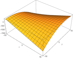
(a) $z=0$.

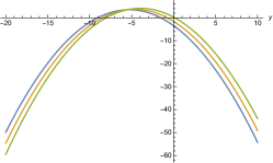
(b) $x=1,2,3,z=0$.

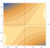
(c) $z=06$.

Figure 1: Parabolic profile for Eq. (41) with parameters $b_{1}=0.54,b_{2}=0.54,k_{3}=5,b_{5}=3,c_{2}=4,c_{1}=5$ and $z=0$.

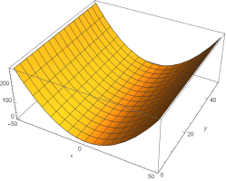
(a) $z=0$.

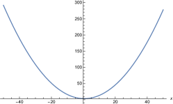
(b) $y=1,z=0$.

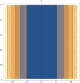
(c) $z=0$.

Figure 2: Parabolic profile for Eq. (42) with free choice of parameters $b_{1}=0.54,b_{2}=0.54,k_{3}=5,b_{5}=3,c_{2}=-4$ and $c_{1}=-5$.

4.2.2 For $f_{1}(Z)=b_{6}$ and $f_{2}(Z)=b_{7}$ with arbitrary constants $b_{6}$ and $b_{7}$ in Eq. (4.2)

Further, Eq. (4.2) recasts in the following form:

$$\xi_{X} =b_{6}+\frac{X}{2}(b_{1}-b_{3}),\,\,\,\,\xi_{Y}=b_{3}Y+b_{4}Z+b_{5},$$

$$\xi_{Z} =b_{1}Z+b_{2},\,\,\,\,\,\,\,\,\,\,\,\,\,\,\,\,\,\,\,\,\,\,\,\,\eta_{F}=b_{7}+\frac{F}{2}(b_{3}-b_{1})+\frac{X}{3}b_{4}.$$ (43)

Case 1: Take $b_{1}\neq 0$ and all other $b_{i}^{\prime}s$ are zero in Eq. (4.2.2), the characteristic equation is

$$\frac{dX}{\frac{X}{2}}=\frac{dY}{0}=\frac{dZ}{Z}=\frac{dF}{-\frac{F}{2}}.$$ (44)

Solving Eqs. (44), we obtain

$$F=\frac{1}{\sqrt{Z}}G(r,s),\,\,\text{with similarity variables are}\,\,\,r=\frac{X}{\sqrt{Z}},\,\,\,s=Y.\,\,\,$$ (45)

Substituting the value of $F$ in Eq. (29), we obtain reduced (1+1)-dimensional nonlinear PDE

$$-2G_{rrrs}+(6G_{rs}-2)G_{r}+(6G_{s}-r)G_{rr}=0.$$ (46)

Infinitesimals for Eq. (46) are

$$\xi_{X}=-\frac{r}{2}\alpha_{1}+\alpha_{3},\,\,\,\xi_{Y}=\alpha_{1}s+\alpha_{2},\,\,\,\eta_{G}=\frac{G}{2}\alpha_{1}+\frac{s}{6}+\alpha_{4},$$ (47)

where $\alpha_{1},\alpha_{2},\alpha_{3}$ and $\alpha_{4}$ are arbitrary constants. Consequently, this case can be categorized into the following subcases:

Case 1A: If $\alpha_{1}\neq 0$ and $\alpha_{2}\neq 0$ in Eq. (47)

Using Eqs. (47), characteristic equation is

$$\frac{dr}{-\frac{r}{2}+\beta_{1}}=\frac{ds}{s+\beta_{2}}=\frac{dG}{\frac{G}{2}+\frac{s}{6}\beta_{1}+\beta_{3}},$$ (48)

where $\beta_{1}=\frac{\alpha_{3}}{\alpha_{1}},\beta_{2}=\frac{\alpha_{2}}{\alpha_{1}}$ and $\beta_{3}=\frac{\alpha_{4}}{\alpha_{1}}$. Solving Eqs. (48), we get similarity variables:

$$G(r,s)=-2\beta_{3}+\frac{1}{3}\beta_{1}(2\beta_{2}+s)+\sqrt{\beta_{2}+s}\,R(w),\,\,\,\,\,\,\text{where}\,\,\,\,\,w=(r-2\beta_{2})\sqrt{\beta_{2}+s}$$ (49)

and $R(w)$ satisfies reduced ODE

$$wR^{(4)}+4R^{(3)}+(w-3R)R^{\prime\prime}-R^{\prime}\left(6wR^{\prime\prime}+6R^{\prime}-2\right)=0$$ (50)

Equation (50) is a nonlinear ordinary differential equation. The authors could not find its general solution. However, three particular solutions of Eq. (50) can be obtained as

$$R(w)=k_{1},\,\,\,\,R(w)=k_{2}+\frac{w}{3},\,\,\,\,R(w)=\frac{k_{3}}{w},\,\,\,\,$$ (51)

where $k_{1},k_{2}$ and $k_{3}$ are integral constants. Using Eqs. (51), (49) and (45) in (28), we obtain the invariant solutions of Eq. (1) are given as

$$u_{7}(x,y,z,t) =\frac{\beta_{1}(2\beta_{2}+y)}{3\sqrt{z}}+k_{1}\sqrt{\frac{\beta_{2}+y}{z}}-\frac{2\beta_{3}}{\sqrt{z}},$$ (52)

$$u_{8}(x,y,z,t) =-\frac{\beta_{1}y}{3\sqrt{z}}+k_{2}\sqrt{\frac{\beta_{2}+y}{z}}+\frac{x(\beta_{2}+y)}{3z}-\frac{2\beta_{3}}{\sqrt{z}},$$ (53)

$$u_{9}(x,y,z,t) =\frac{\beta_{1}(2\beta_{2}+y)}{3\sqrt{z}}+\frac{k_{3}}{x-2\beta_{1}\sqrt{z}}-\frac{2\beta_{3}}{\sqrt{z}}.$$ (54)

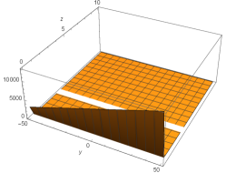
(a) $x=15$

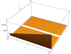
(b) $x=18$

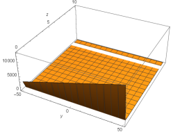
(c) $x=24$

Figure 3: Movable singularity profile for Eq. (54) with parameters $b_{1}=4,b_{3}=1,b_{2}=40,k_{2}=-1$ and $k_{3}=-5$.

Case 1B:  For $\alpha_{1}=0$, and $\alpha_{2}\neq 0$ in Eq. (47)

In this case, characteristic equations is

$$\frac{dr}{\alpha_{3}}=\frac{ds}{\alpha_{2}}=\frac{dG}{\frac{s}{6}\alpha_{3}+\alpha_{4}}.$$ (55)

Solving Eqs. (55), we obtain similarity variables as

$$G(r,s)=\frac{\alpha_{4}}{\alpha_{2}}s+\frac{\alpha_{3}}{\alpha_{2}}\frac{s^{2}}{12}+R(w),\,\,\,\,\,\,\text{where}\,\,\,\,\,w=r-\frac{\alpha_{3}}{\alpha_{2}}s,$$ (56)

and $R(w)$ satisfies reduced ODE

$$2R^{\prime}\left(\alpha_{2}+6\alpha_{3}R^{\prime\prime}\right)+(\alpha_{2}w-6\alpha_{4})R^{\prime\prime}-2\alpha_{3}R^{(4)}=0.$$ (57)

Two particular solutions of Eq. (57) can be furnished as

$$R(w)=k_{1},\,\,\,\,R(w)=k_{2}-\frac{\alpha_{2}w^{2}}{8\alpha_{3}}+\frac{3\alpha_{4}w}{2\alpha_{3}}$$ (58)

where $k_{1}$ and $k_{2}$ are constant of integration. Using Eqs. (58), (56), (45) in (28), we obtain the invariant solutions of Eq. (1) is given as

$$u_{10}(x,y,z,t) =\frac{k_{1}}{\sqrt{z}}+\frac{\alpha_{3}y^{2}+12\alpha_{4}y}{12\alpha_{2}\sqrt{z}}$$ (59)

$$u_{11}(x,y,z,t) =\frac{1}{\sqrt{z}}\left(k_{2}+\frac{\alpha_{4}}{\alpha_{2}}y++\frac{\alpha_{3}y^{2}}{12\alpha_{2}}+\frac{3\alpha_{4}}{{2\alpha_{3}}}\left(\frac{x}{\sqrt{z}}-\frac{\alpha_{3}y}{\alpha_{2}}\right)-\frac{\alpha_{2}}{{8\alpha_{3}}}\left(\frac{x}{\sqrt{z}}-\frac{\alpha_{3}y}{\alpha_{2}}\right)^{2}\right)$$ (60)

4.2.3 For $f_{1}(Z)=f_{2}(Z)=0$ and $b_{1}=b_{3}=0$ in Eq (4.2).

In this case, characteristic equation for Eq. (4.2) reduces to

$$\frac{dX}{0}=\frac{dY}{b_{4}Z+b_{5}}=\frac{dZ}{b_{2}}=\frac{dF}{\frac{X}{3}b_{4}}.$$ (61)

Solving Eqs. (61), we obtain variables

$$F=\frac{b_{4}}{3b_{2}}XZ+G(r,s),\,\,\text{where}\,\,r=X\,\,\text{and}\,\,\,s=Y-\frac{b_{4}}{2b_{2}}Z^{2}-\frac{b_{5}}{b_{2}}Z,\,\,b_{2}\neq 0$$ (62)

and $G(r,s)$ satisfies reduced (1+1)-dimensional PDE

$$b_{4}-3(b_{5}-3b_{2}G_{r})G_{rs}+9b_{2}G_{s}G_{rr}-3b_{2}G_{rrrs}=0$$ (63)

Using new infinitesimals for Eq. (63), characteristic equations is given as

$$\frac{dr}{-\frac{r}{4}d_{1}+d_{3}}=\frac{ds}{d_{1}s+d_{2}}=\frac{dF}{\frac{G}{4}d_{1}-\frac{b_{5}r}{6b_{2}}d_{1}+d_{4}}$$ (64)

Consequently, two cases are discussed below:
Case 1: $d_{1}\neq 0:$
By solving Eqs. (64) we obtain similarity variables as

$$G=\frac{4d_{4}r}{4d_{3}-d_{1}r}-\frac{b_{5}d_{1}r^{2}}{3b_{2}(4d_{3}-d_{1}r)}+\frac{R(w)}{4d_{3}-d_{1}r},\,\,\,\,\,\text{where}\,\,\,\,\,w=\frac{\sqrt[4]{d_{1}s+d_{2}}(d_{1}r-4d_{3})}{d_{1}}.$$ (65)

Here, $R(w)$ satisfies ODE

$$w\left(d_{1}^{2}w^{2}\left(3b_{2}R^{(4)}+4b_{4}\right)+3R^{\prime\prime}(16d_{3}(b_{5}d_{3}-3b_{2}d_{4})-3b_{2}d_{1}R)\right)$$

$$+6R^{\prime}\left(3b_{2}d_{1}\left(w^{2}R^{\prime\prime}+R\right)-16d_{3}(b_{5}d_{3}-3b_{2}d_{4})\right)-18b_{2}d_{1}wR^{\prime 2}=0.$$ (66)

Eq. (4.2.3) is highly nonlinear and very difficult to solve in general. But we found one particular solution which is given below:

$$R(w)=\pm\frac{i\sqrt{2}\sqrt{b_{4}}\sqrt{d_{1}}}{3\sqrt{b_{2}}}w^{2}+k_{4}w-\frac{16\left(3b_{2}d_{3}d_{4}-b_{5}d_{3}^{2}\right)}{3b_{2}d_{1}},$$ (67)

where $k_{4}$ is an arbitrary constant. Then, invariant solution is given by

$$\noindent u_{12}(x,y,z,t)=\frac{\pm i\sqrt{2}\sqrt{b_{2}}\sqrt{b_{4}}\sqrt{d_{1}s+d_{2}}(d_{1}r-4d_{3})-3b_{2}\sqrt{d_{1}}\left(k_{4}\sqrt[4]{d_{1}s+d_{2}}+4d_{4}\right)+b_{4}d_{1}^{3/2}xz+b_{5}\sqrt{d_{1}}(d_{1}r+4d_{3})}{3b_{2}d_{1}^{3/2}}$$ (68)

where $r$ and $s$ are given by Eq. (62).

Case 2: $d_{1}=0:$
On solving Eqs. (64), the group invariant form is obtained as

$$G=\frac{d_{4}s}{d_{2}}+R(w)\,\,\text{with}\,\,w=r-\frac{d_{3}s}{d_{2}},\,\,d_{2}\neq 0,$$ (69)

where $R(w)$ satisfies reduced ODE

$$3b_{2}d_{3}R^{(4)}+3R^{\prime\prime}\left(-6b_{2}d_{3}R^{\prime}+3b_{2}d_{4}+b_{5}d_{3}\right)+b_{4}d_{2}=0.$$ (70)

Taking $d_{3}=0$ in Eq. (70), we get

$$R(w)=-\frac{b_{4}d_{2}w^{2}}{18b_{2}d_{4}}+k_{2}w+k_{1},$$ (71)

where $k_{1}$ and $k_{2}$ are constant of integration. Then, the invariant solution of Eq. (1) is given as

$$u_{13}(x,y,z,t)=\frac{d_{4}}{d_{2}}s-\frac{b_{4}d_{2}}{18b_{2}d_{4}}x^{2}+\frac{b_{4}}{3b_{2}}xz+k_{2}x+k_{1},$$ (72)

where $s$ is given by Eq. (62).

4.3 Vector field $v_{3}$:

For the associated vector field

$$v_{3}=y\frac{\partial}{\partial y}+z\frac{\partial}{\partial z}$$

corresponding characteristic equation is

$$\frac{dx}{0}=\frac{dy}{y}=\frac{dz}{z}=\frac{dt}{0}=\frac{du}{0}.$$ (73)

Solving Eqs. (73) we obtain the group invariant form

$$u=F(X,Y,T),\,\,\,\text{where similarity variables are}\,\,\,X=x,\,\,\,Y=\frac{y}{z},\,\,\,T=t.\,\,\,$$ (74)

Substituting Eq. (74) in Eq. (1), we obtain the reduced (2+1)-dimensional nonlinear PDE:

$$F_{YT}+(Y-3F_{X})F_{XY}-3F_{Y}F_{XX}+F_{XXXY}=0.$$ (75)

To find invariant solutions for shallow water wave equation (1), we obtain the infinitesimals for Eq. (75)

$$\xi_{X} =\frac{X}{3}b_{1}+f_{1}(T),\,\,\,\,\,\,\,\,\xi_{Y}=\frac{-2Y}{3}b_{1}+b_{3},$$

$$\xi_{T} =b_{1}T+b_{2},\,\,\,\,\,\,\,\,\,\,\,\,\,\,\,\,\,\,\,\,\eta_{F}=\frac{-F}{3}b_{1}+\frac{X}{3}(b_{3}-f_{1}^{\prime}(T))+f_{2}(T).$$ (76)

where $b_{1},b_{2},b_{3}$ are arbitrary constants and $f_{1}(T),f_{2}(T)$ are arbitrary functions. We can assume $f_{1}(T)=b_{3}T+b_{4}$ and $f_{2}(T)=b_{5}$, where $b_{3},b_{4}$ and $b_{5}$ are arbitrary constants.
Consequently, following two subcase arise:
Case 1: If $b_{1}\neq 0$, the corresponding Lagrange’s system comes into existence for Eq. (75)

$$\frac{dX}{\frac{X}{3}+c_{1}T+c_{2}}=\frac{dY}{\frac{-2Y}{3}+c_{1}}=\frac{dT}{T+c_{3}}=\frac{dF}{\frac{-F}{3}+c_{4}},$$ (77)

where $c_{1}=\frac{b_{3}}{b_{1}},c_{2}=\frac{b_{4}}{b_{1}},c_{3}=\frac{b_{2}}{b_{1}}$ and $c_{4}=\frac{b_{5}}{b_{1}}$. Solving Eq. (77), we obtain

$$F=\frac{G(r,s)}{\sqrt[3]{c_{3}+t}}+3c_{4},\,\,\,\text{where}\,\,\,\,r=\frac{2x-9c_{1}c_{3}-3c_{1}t+6c_{2}}{2\sqrt[3]{c_{3}+t}}\,\,\text{and}\,\,s=-\frac{1}{2}(3c_{1}-2y)(c_{3}+t)^{2/3}.$$ (78)

Also, $G(r,s)$ satisfies following (1+1)-dimensional PDE

$$2sG_{ss}+G_{s}(1-9G_{rr})+3G_{rrrs}-(r-3s+9G_{r})G_{rs}=0.$$ (79)

The general solution of Eq. (79) is difficult to obtain. But using Lie symmetry method, we can find new set of infinitesimals for Eq. (79). Hence, we can write corresponding characteristic equation:

$$\frac{dr}{\alpha_{1}}=\frac{ds}{0}=\frac{dG}{\frac{-r}{9}\alpha_{1}+\alpha_{2}}.$$ (80)

Solving Eqs. (80), we obtain following invariant

$$G(r,s)=\frac{\alpha_{2}r}{\alpha_{1}}-\frac{r^{2}}{18}+R(w)\,\,\text{where}\,\,w=s,\,\,\,\alpha_{1}\neq 0,$$ (81)

where $R(w)$ satisfies the reduced ODE

$$R^{\prime}+wR^{\prime\prime}=0.$$ (82)

Two particular solutions of Eq. (82) are given below

$$R(w)=k_{1}\,\,\,\text{and}\,\,\,R(w)=k_{2}+k_{3}\log(w),$$ (83)

where $k_{1},k_{2}$ and $k_{3}$ are constant of integration. Using Eqs. (83), (81) and (78) in (74), we get the invariant solutions of Eq. (1)

$$u_{14}(x,y,z,t)=- \frac{\left(-3c_{1}\left(3c_{3}+t\right)+6c_{2}+2x\right)\left(a_{1}\left(-3c_{1}\left(3c_{3}+t\right)+6c_{2}+2x\right)-36a_{2}\sqrt[3]{c_{3}+t}\right)}{72a_{1}\left(c_{3}+t\right)}$$

$$+\frac{k_{1}}{\sqrt[3]{c_{3}+t}}+\frac{3c_{4}}{\sqrt[3]{c_{3}+t}},$$ (84)

$$u_{15}(x,y,z,t)= \frac{1}{\sqrt[3]{c_{3}+t}}\left(\frac{\alpha_{2}}{\alpha_{1}}r+k_{2}\log\left[\left(\frac{2y-3zc_{1}}{2z}\right)(c_{3}+t)^{2/3}\right]+k_{3}-\frac{r^{2}}{18}\right)+3c_{4},$$ (85)

where $r$ is given by Eq. (78)

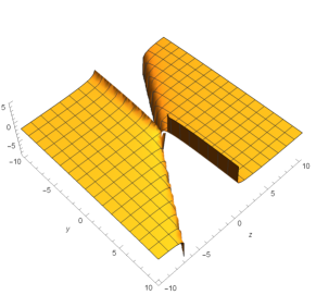
(a) $x=3$.

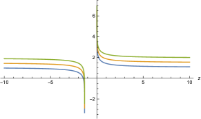
(b) $x=3,y=2$.

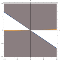
(c) $x=3$.

Figure 4: Cross kink soliton solution for for Eq. (4.3) with parameters $t=0,c_{1}=-1,c_{2}=1,c_{3}=10,c_{4}=1,k_{1}=1,k_{2}=1,k_{3}=1,a_{1}=5,a_{2}=5,x=3$. (a) 3D profile for $-10<y<10,-10<z<10$. (b) wave propagation along $z$ axis. (c) corresponding contour plot.

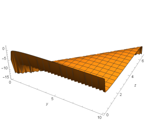
(a) $x=3$.

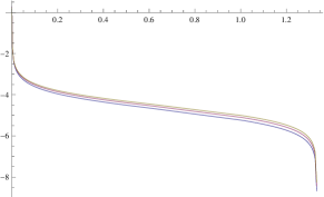
(b) $x=3,y=2$.

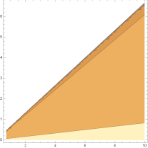
(c) $x=3$.

Figure 5: Cross kink soliton solution for Eq. (4.3) with parameters $t=0,c_{1}=1,c_{2}=1,c_{3}=10,c_{4}=1,k_{1}=1,k_{2}=1,k_{3}=1,a_{1}=5,a_{2}=5,x=3$. (a) 3D profile for $0<y<10,0<z<10$. (b) wave propagation along $z$ axis. (c) corresponding contour plot.

Case 2: If $b_{1}=0$, the resulting Lagrange’s system takes the form

$$\frac{dX}{b_{3}T+b_{4}}=\frac{dY}{b_{3}}=\frac{dT}{b_{2}}=\frac{dF}{b_{5}}.$$ (86)

Solving Eq. (86), we get

$$F=\frac{b_{5}}{b_{2}}T+G(r,s),\,\,\,\text{where}\,\,\,\,r=x-\frac{1}{2b_{2}}(2b_{4}+b_{3}T)T\,\,\text{and}\,\,s=Y-\frac{b_{3}}{b_{2}}T.$$ (87)

where $G(r,s)$ satisfies PDE

$$b_{2}(G_{rrrs}-3G_{s}G_{rr})-b_{3}G_{ss}-(b_{4}-b_{2}s+3b_{2}G_{r})G_{rs}=0.$$ (88)

To solve Eq. (88), we found new set of infinitesimals:

$$\xi_{r}=c_{2},\,\,\xi_{s}=c_{1},\,\,\text{and}\,\,\eta_{G}=\frac{1}{3}rc_{1}+c_{3}.$$ (89)

where $c_{1},c_{2}$ and $c_{3}$ are arbitrary constants. After solving characteristic equations we obtain group invariant form

$$G=\frac{r^{2}}{6}\frac{c_{1}}{c_{2}}+\frac{c_{3}}{c_{2}}r+R(w)\,\,\text{where}\,\,w=r-\frac{c_{2}}{c_{1}}s,\,\,\,c_{1}\neq 0,c_{2}\neq 0.$$ (90)

where $R(w)$ satisfies reduced ODE

$$R^{\prime\prime}\left(b_{2}c_{1}(c_{1}w+3c_{3})-b_{3}c_{2}^{2}+b_{4}c_{1}c_{2}\right)-b_{2}c_{1}c_{2}R^{(4)}+b_{2}c_{1}R^{\prime}\left(c_{1}+6c_{2}R^{\prime\prime}\right)=0$$ (91)

where ’ is derivaitve with respect to $w$. Integrating Eq. (91)

$$R^{\prime}\left(3b_{2}c_{1}c_{2}R^{\prime}+b_{2}c_{1}(c_{1}w+3c_{3})-b_{3}c_{2}^{2}+b_{4}c_{1}c_{2}\right)-b_{2}c_{1}c_{2}R^{(3)}=c_{0}$$ (92)

where $c_{0}$ is constant of integration. Eq. (92) is a complicated nonlinear differential equation and cannot be solved in general. Anyhow assuming the adequate values of arbitrary constants, some particular results can be attained in the following manner:

$$R(w)=k_{1}\,\,\,\text{and}\,\,\,R(w)=k_{2}+\frac{A}{3b_{2}c_{1}c_{2}}w-\frac{c_{1}}{6c_{2}}w^{2}$$ (93)

where $k_{1},k_{2}$ are arbitrary constants and $A=-3b_{2}c_{1}c_{3}+b_{3}c_{2}^{2}-b_{4}c_{1}c_{2}$.

Using Eqs. (93), (90) (87) in (74), we obtain the invariant solutions of Eq. (1) which are given as

$$u_{16}(x,y,z,t) =\frac{1}{24b_{2}^{2}c_{2}}\left(-2b_{2}x+b_{3}t^{2}+2b_{4}t\right)(c_{1}t(b_{3}t+2b_{4})-2b_{2}(c_{1}x+6c_{3}))+\frac{b_{5}t}{b_{2}}+k_{1},$$ (94)

$$u_{17}(x,y,z,t) =\frac{Aw}{3b_{2}c_{1}c_{2}}+\frac{b_{5}t}{b_{2}}+\frac{r(c_{1}r+6c_{3})}{6c_{2}}-\frac{c_{1}w^{2}}{6c_{2}}+k_{3},$$ (95)

where $w$ is given by Eq. (90) and $r,s$ are given by Eq. (87).

4.4 Vector field $v_{4}$:

For the associated vector field

$$v_{4}=\frac{\partial}{\partial z},$$

correspoding characteristic equation is

$$\frac{dx}{0}=\frac{dy}{0}=\frac{dz}{1}=\frac{dt}{0}=\frac{du}{0}.$$ (96)

By solving Eq. (96), we get

$$u=F(X,Y,T),\,\,\,\text{with similarity variables are}\,\,\,X=x,\,\,\,Y=y,\,\,\,T=t,\,\,\,$$ (97)

where $F$ satisfies the reduced (2+1)-dimensional nonlinear PDE

$$F_{XXXY}-3F_{X}F_{XY}-3F_{Y}F_{XX}+F_{YT}=0.$$ (98)

The reduced Eq. (98) is well known (2+1)-dimensional Boiti–Leon–Manna–Pempinelli (BLMP) equation was recently tackled by many researchers [33, 36, 37, 38, 39, 40, 41, 42, 43]. Recently, Kumar and Tiwai [33] applied Lie symmetry approach to find explicit solutions of BLMP equation and found exact and closed form solutions of Eq. (98), such as, parabolic, periodic, quasi periodic, multisoliton and asymptotic type solutions.

4.5 Vector field $v_{5}$:

For the associated vector field

$$v_{5}=\frac{t}{2}\frac{\partial}{\partial x}+z\frac{\partial}{\partial y}+\frac{x}{6}\frac{\partial}{\partial u},$$

correspoding characteristic equation is

$$\frac{dx}{\frac{t}{2}}=\frac{dy}{z}=\frac{dz}{0}=\frac{dt}{0}=\frac{du}{\frac{x}{6}}.$$ (99)

Solving Eq. (99), we obtain the group invariant form

$$u=F(X,Z,T),\,\,\,\text{where similarity variables are}\,\,\,X=x-\frac{ty}{2z},\,\,\,Z=z,\,\,\,T=t,\,\,\,$$ (100)

where $F$ satisfies the reduced (2+1)-dimensional nonlinear PDE

$$TF_{XT}+2ZF_{XZ}-6TF_{X}F_{XX}-XF_{XX}+TF_{XXXX}=0.$$ (101)

For Eq. (101) new set of infinitesimals

$$\xi_{X} =\frac{1}{2}XZf_{2}(A)+\frac{1}{3A}Xf_{3}(A)+\sqrt{Z}f_{5}(A)+\frac{1}{\sqrt{Z}}f_{4}(A),$$

$$\xi_{Z} =Z^{2}f_{2}(A)+Zf_{1}(A),$$

$$\xi_{T} =\frac{1}{2}ZTf_{2}(A)+\sqrt{Z}f_{3}(A),$$

$$\eta_{F} =\frac{1}{6T}\left(-3TZFf_{2}(A)-X^{2}Zf_{2}(A)-2X\sqrt{Z}f_{5}(A)-2F\sqrt{Z}f_{3}(A)+6Tf_{6}(Z,T)\right),$$ (102)

where $A=\frac{T}{\sqrt{Z}}$ and $f_{1},f_{2},f_{3},f_{4},f_{5}$ are arbitrary functions. Taking $f_{1}(A)=b_{1},f_{2}(A)=0,f_{3}(A)=3b_{2}A,f_{4}(A)=0,f_{5}(A)=3b_{3}A$ and $f_{6}(A)=0$. After putting values of arbitrary function infinitesimals (4.5) takes the form

$$\xi_{X} =b_{2}X+3b_{3}T,$$

$$\xi_{Z} =b_{Z},$$

$$\xi_{T} =3b_{2}T,$$

$$\eta_{F} =-b_{3}X-b_{2}F,$$ (103)

where $b_{1},b_{2},b_{3}$ are arbitrary constants. Take $b_{3}\neq 0$ all other $b_{i}$’s zero in Eq. (4.5). Lagrange system recast as

$$\frac{dX}{3T}=\frac{dZ}{0}=\frac{dT}{0}=\frac{dF}{-X}.$$ (104)

Solving Eq. (104) we obtain similarity variables

$$F=-\frac{X^{2}}{6T}+G(r,s)\,\,\,\text{where}\,\,r=Z\,\,\text{and}s=T.$$ (105)

Substituting Eq. (105) in (101) we found it satisfies the Eq. (101). Hence invariant solution for Eq. (1) is

$$u_{18}(x,y,z,t)=-\frac{1}{6t}\left(x-\frac{ty}{2z}\right)^{2}+G(z,t)$$ (106)

where $G$ is an arbitrary function with rich physical interpretation as shown in Fig. 6 for $G(z,t)=\sin(z^{2}t)$ and 7 for $f(z,t)=sech(z^{2}t)$.

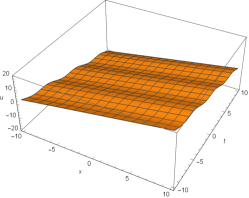
(a) $y=5,z=1$.

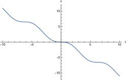
(b) $y=5,z=1$.

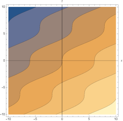
(c) $y=5,z=1$.

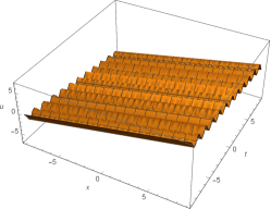
(d) $y=5,z=3$.

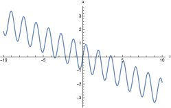
(e) $y=5,z=3$.

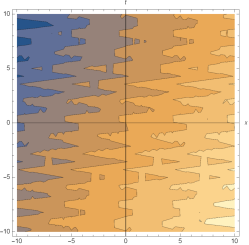
(f) $y=5,z=3$.

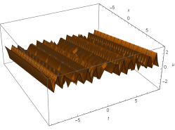
(g) $y=5,z=5$.

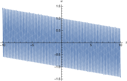
(h) $y=5,z=5$.

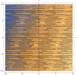
(i) $y=5,z=5$.

Figure 6: Multisoliton and Solitary wave solutions profile of Eq. (106) to different values of $t$ for free choice of function $G(z,t)=\sin(z^{2}t)$. (a), (d), (g) show evolution of multisoliton; (b), (e), (h) show the wave propagation pattern of the wave along the $t$-axis; (c), (f), (i) show corresponding contour plot.

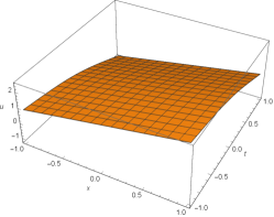
(a) $y=5,z=1$.

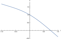
(b) $y=5,z=1$.

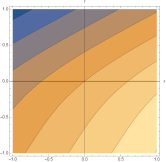
(c) $y=5,z=1,x=0$.

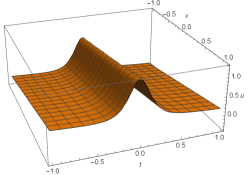
(d) $y=5,z=3$.

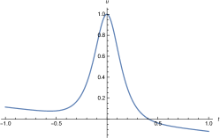
(e) $y=5,z=3$.

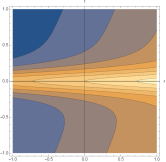
(f) $y=5,z=3,x=0$.

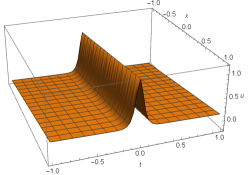
(g) $y=5,z=5$.

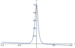
(h) $y=5,z=5$.

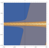
(i) $y=5,z=5,x=0$.

Figure 7: Solitary wave profile of Eq. (106) for function $G(z,t)=sech(z^{2}t)$. (a) Single soliton. Figs. (a), (d), (g) show Single soliton. Figs. (b), (e), (h) show the wave propagation pattern of the wave along the $t$-axis. Figs. (c), (f), (i) show correspoding coutour plot.

4.6 Vector field $v_{6}$:

For the associated vector field

$$v_{6}=\frac{\partial}{\partial y}$$

correspoding Lagrange system is

$$\frac{dx}{0}=\frac{dy}{1}=\frac{dz}{0}=\frac{dt}{0}=\frac{du}{0}.$$ (107)

Solving Eq. (107), we get

$$u=F(X,Z,T),\,\,\,\text{where similarity variables are}\,\,\,X=x,\,\,\,Z=z,\,\,\,T=t.\,\,\,$$ (108)

where $F$ satisfies the reduced PDE

$$-F_{XZ}=0$$ (109)

The general solution of Eq. (109) is

$$F(X,Z,T)=f_{1}(X,T)+f_{2}(Z,T)$$ (110)

where $f_{1}$ and $f_{2}$ are arbitrary functions. Hence, the invariant solution of Eq. (1) is given as

$$u_{19}(x,y,z,t)=f_{1}(x,t)+f_{2}(z,t)$$ (111)

where $f_{1}$ and $f_{2}$ are arbitrary functions.

4.7 Vector field $v_{7}$:

For the associated vector field

$$v_{7}=t\frac{\partial}{\partial x}-\frac{x}{3}\frac{\partial}{\partial u},$$

correspoding Lagrange system is

$$\frac{dx}{t}=\frac{dy}{0}=\frac{dz}{0}=\frac{dt}{0}=\frac{du}{\frac{-x}{3}}.$$ (112)

Solving Eq. (112) we obtain the group invariant form

$$u=\frac{-x^{2}}{6t}+F(Y,Z,T),\,\,\,\text{where similarity variables are}\,\,\,Y=y,\,\,\,Z=z,\,\,\,T=t.$$ (113)

where $F$ satisfies the reduced PDE

$$F_{Y}+TF_{YT}=0$$ (114)

Equation (114) has general solution

$$F(Y,Z,T)=\frac{1}{T}f_{1}(Y,Z)+f_{2}(Z,T)$$ (115)

where $f_{1}$ and $f_{2}$ are arbitrary functions. Hence, the invariant solution of Eq. (1) is given as

$$u_{20}(x,y,z,t)=-\frac{x^{2}}{6t}+\frac{1}{t}f_{1}(y,z)+f_{2}(z,t).$$ (116)

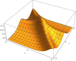
(a) $x=5,t=1$.

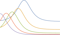
(b) $x=5,t=1,z=1,2,3,4,5$.

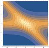
(c) $x=5,t=1$.

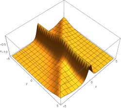
(d) $x=5,t=3$.

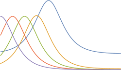
(e) $x=5,t=3,z=1,2,3,4,5$.

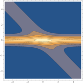
(f) $x=5,t=3$.

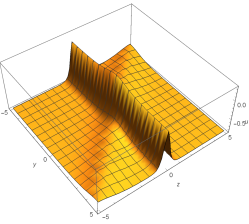
(g) $x=5,t=5$.

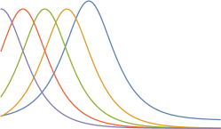
(h) $x=5,t=5,z=1,2,3,4,5$.

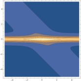
(i) $x=5,t=5$.

Figure 8: Doubly periodic breather-type solution profile of Eq. (116) for free function $f_{1}(z,t)=sech(z\,t),f_{2}(y,z)=sech(y+z)$. Figs. (a), (d), (g) show Single soliton. Figs. (b), (e), (h) show the wave propagation pattern of the wave along the $y$-axis. Figs. (c), (f), (i) show correspoding coutour plot.

4.8 Vector field $v_{8}$:

For the associated vector field

$$v_{8}=\frac{\partial}{\partial x},$$

correspoding Lagrange system is

$$\frac{dx}{1}=\frac{dy}{0}=\frac{dz}{0}=\frac{dt}{0}=\frac{du}{0}.$$ (117)

Solving Eq. (117), we get

$$u=F(Y,Z,T),\,\,\,\text{where similarity variables are}\,\,\,Y=y,\,\,\,Z=z,\,\,\,T=t.$$ (118)

The reduced PDE

$$-F_{YT}=0,$$ (119)

has general solution as

$$F(Y,Z,T)=f_{1}(Y,Z)+f_{2}(Z,T),$$ (120)

where $f_{1}$ and $f_{2}$ are arbitrary functions. Using Eqs. (120) in (118), we obtain the invariant solution of Eq. (1) as

$$u_{21}(x,y,z,t)=f_{1}(y,z)+f_{2}(z,t).$$ (121)

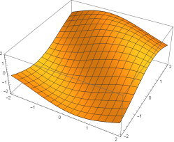
(a) $t=1$.

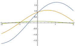
(b) $t=1,y=1,2,3$.

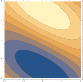
(c) $t=1$.

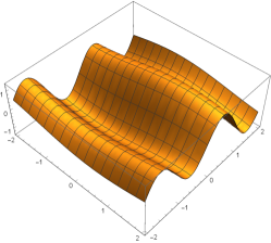
(d) $t=3$.

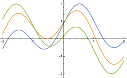
(e) $t=3,y=1,2,3$.

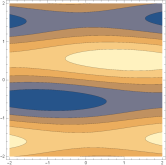
(f) $t=3$.

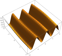
(g) $t=5$.

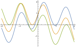
(h) $t=5,y=1,2,3$.

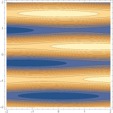
(i) $t=5$.

Figure 9: The solitary wave solution profiles of Eq. (121) for particular function $f_{1}(z,t)=\sin(zt),f_{2}(y,z)=\sin(y+z)$. Figs. (a), (d), (g) shows evolution of solitary waves; Figs. (b), (e), (h) gives wave propagation pattern of the wave along the $y$-axis; Figs. (c), (f), (i) shows corresponding contour plot.

5 Results and discussion

This study provides soliton solutions, rational solutions through symmetry analysis for the GSWW equation with constant-dependent coefficients. Many researchers have studied GSWW equation using different techniques. Overall we have obtained 21 invairant solutions corresponding to vector fields. We presented Lie symmetries and similarity reductions by constructing group-invariant solutions from the 12-dimensional Lie algebras while in one of Lie algebra reduced into well-known BLMP equation. Various new periodic solitary wave solutions are successfully constructed. Moreover, graphical representation of the solutions $u_{5},u_{6},u_{9},u_{14},u_{18},u_{20}$ and $u_{21}$ are analyzed physically in figures 1, 2, 3, 4, 5, 6, 7, 8, 9. We framed the 2D, 3D and the contour graphics to some of the attained solutions. In our study, we present some new soliton solutions which are invariant for GSWW equation that could not be obtained earlier. Moreover, some new information about GSWW equation are presented from the perspective of Lie symmetry analysis.

6 Conclusion

In this article, we study the (3+1)-dimensional generalized shallow water wave equation to find closed form solutions via Lie symmetry method. We have discussed infinite-dimensional Lie algebra and commutation relations for the equation. With the symbolic calculations and the reported results in this research, we have seen that the Lie symmetry method is well-organized and reliable mathematical tools that can be used to examine various nonlinear evolution equations arising in the different fields of marine environment, plasma physics and nonlinear science. Entire computational calculations in this article are carried out with aid of Maple 15 and Wolfram Mathematica 11.

Author contribution statement

Both Authors contributed equally to this work.

Compliance with ethical standards

Conflict of interest The authors declare that they have no conflict of interest.

References

- [1] M S Khatun, M F Hoque and M A Rahman Pramana - J. Phys. 88 86 (2017)
- [2] A Biswas Commun. Nonlinear Sci. Numer. Simul. 14 2524 (2009)
- [3] A M Wazwaz Chaos Solitons Fractals 76 93 (2015)
- [4] S T R Rizvi, K Ali, A Sardar, M Younis and A Bekir Pramana - J. Phys. 88 16 (2017)
- [5] H C Jin, D Lee and H Kim J. Phys. 87 55 (2016)
- [6] R P Chen and C Q Dai Nonlinear Dyn. 88 2807 (2017)
- [7] D J Ding, D Q Jin and C Q Dai Therm. Sci. 21 1701 (2017)
- [8] M J Ablowitz and P A Clarkson Solitons, nonlinear evolution equations and inverse scattering (New York: Cambridge Univ. Press) (1991)
- [9] J G Liu, Y Z Li and G M Wei Chin. Phys. Lett. 23 1670 (2006)
- [10] R Hirota Phys. Rev. Lett. 27 1192 (1971)
- [11] E Fan and H Zhang Phys. Lett. A 246 403 (1998)
- [12] E Fan Phys. Lett. A 265 353 (2000)
- [13] M Senthilvelan Appl. Math. Comput. 123 381 (2001)
- [14] S Zhang Chaos Solitons Fractals 30 1213 (2006)
- [15] C Q Dai, Y Y Wang and J F Zhang Opt. Lett. 35 1437 (2010)
- [16] J G Liu, Z F Zeng, Y He and G P Ai Int. J. Nonlin. Sci. Num. 19 37 (2014)
- [17] Z F Zeng, J G Liu and B Nie Nonlinear Dyn. 86 667 (2016)
- [18] B Tian and Y T Gao Comput. Phys. Commun. 95 139 (1996)
- [19] E M E Zayed J. Appl. Math. Inform. 28 383 (2010)
- [20] Y N Tang, W X Ma and W Xu Chin. Phys. B 21 070212 (2012)
- [21] C B Vreugdenhil Numerical Methods for Shallow–Water Flow (The Netherlands: Kluwer Academic Publishers) (1994)
- [22] J G Liu and Y He Nonlinear Dyn. 90 363 (2017)
- [23] Y Z Li and J G Liu Pramana – J. Phys. 90, 71 (2018)
- [24] X H Meng Comp. Math. Appl. 75 4534 (2018)
- [25] P A Clarkson and E L Mansfield Nonlinearity 7 915 (1994)
- [26] R Hirota Phys. Rev. Lett. 27 1192 (1971)
- [27] G W Bluman and S Kumei Symmetries and Differential Equations (New York: Springer) (1989)
- [28] P Hydon Symmetry Methods for Differential Equations: A Beginner’s Guide (Cambridge: Cambridge University Press) (2000)
- [29] L V Ovsiannikov Group Analysis of Differential Equations (New York: Academic Press Inc.) (1982)
- [30] S Kumar and Y K Gupta Int. J. Theor. Phys. 53 2041 (2014)
- [31] S Kumar, Pratibha and Y K Gupta Int. J. Mod. Phys. A 25 3993 (2010)
- [32] M Kumar, R Kumar and A K Kumar Comput. Math. Appl. 68 454 (2018)
- [33] M Kumar and A K Tiwari Comput. Math. Appl. 75 1434 (2018)
- [34] P J Olver Applications of Lie Groups to Differential Equations (New York: Springer) (1986).
- [35] M B Kochanov, N A Kudryashov and D I Sinel’shchikov J. Appl. Math. Mech. 77 25 (2003)
- [36] Y Li and D Li Appl. Math. Sci. 6 579 (2012)
- [37] L Luo Phys. Lett. A 375 1059 (2011)
- [38] S Mabrouk and M Kassem Ain Shams Eng. J. 5 227 (2014)
- [39] Y Tang and W Zai Nonlinear Dyn. 81 249 (2015)
- [40] A S Alofi and M A Abdelkawy Life Sci. J. 9 3995 (2012)
- [41] X Deng, H Chen and Z Xu J. Math. Res. 6 85 (2014)
- [42] L Delisle and M Mosaddeghi J. Phys. A: Math. Theor. 46 115203 (2013)
- [43] C J Bai and H Zhao Modern Phys. B 22 2407 (2008)