A Hubbard model with integrable impurity

Abstract

We construct an integrable Hubbard model with impurity site containing spin and charge degrees of freedom. The Bethe ansatz equations for the Hamiltonian are derived and two alternative sets of equations for the thermodynamical properties. For this study, the thermodynamical Bethe ansatz and the quantum transfer matrix approach are used. The latter approach allows for a consistent treatment by use of a finite set of non-linear integral equations. In both cases, TBA and QTM, the contribution of the impurity to the thermodynamical potential is given by integral expressions.

I Introduction

The history of the Hubbard model as an exactly solvable model started in $1968$ with Lieb and Wu’s article Lieb and Wu (1968). The consistency of the Bethe Ansatz, i.e. absence of multi-particle processes was shown by Essler and Korepin Essler and Korepin (1994a, b) and transparently by the embedding of the Hubbard model into a formulation with commuting transfer matrices by the work of Shastry Shastry (1986a). Following this, the algebraic Bethe ansatz constructions of the eigenstates were given by Martins Ramos and Martins (1997); Martins and Ramos (1998).

Lieb and Wu demonstrated that the Bethe ansatz can be used which reduces the eigenvalue problem of the Hamiltonian to solving a set of coupled algebraic equations, which are called Lieb-Wu equations. They calculated the ground state energy and discovered that the Hubbard model undergoes a Mott metal-insulator transition at half filling (on average one electron per site) with critical interaction strength $U=0$.

A classification of the solutions of the Lieb-Wu equations in terms of the so-called string hypothesis was given by Takahashi in 1972 Takahashi (1972). He used this to replace the Lieb-Wu equations by simpler ones that describe the scattering states of bound complexes (strings), and derived the thermodynamic Bethe ansatz (TBA) equations, which determine the Gibbs free energy of the Hubbard model. From the TBA, in the limit of low temperatures, Takahashi calculated the specific heat Takahashi (1974). Subsequently a rather reliable picture of the thermodynamics of the Hubbard model was derived from numerical solutions of the thermodynamic Bethe ansatz equations Kawakami et al. (1989); Usuki et al. (1990). As a matter of fact, Takahashi’s equations, in conjunction with the thermodynamic Bethe ansatz equations, can be utilizied to calculate any physical quantity that pertains to the energy spectrum. There are constraints on the quantum numbers in Takahashi’s equations which imply particular selection rules that determine the permitted combinations of elementary excitations and hence the physical excitation spectrum Deguchi et al. (2000). Takahashi’s equations can also be used as the starting point for the calculation of the scattering matrix of the elementary excitations. For the half-filled Hubbard model in vanishing magnetic field the $S$-matrix was calculated Essler and Korepin (1994a, b). The excitation spectrum at half filling is given by scattering states of four elementary excitations: holon and antiholon with spin $0$ and charge $\pm e$ and charge neutral spinons with spin up or down, respectively. This is noteworthy, because away from half filling, or at finite magnetic field, the number of elementary excitations is infinite Deguchi et al. (2000). Furthermore the four particles can only be excited in $SO\left(4\right)$ multiplets Essler and Korepin (1994a, b); Essler et al. (2005).

In $1986$ Shastry started a novel way for studying the Hubbard model by embedding it into the framework of the quantum inverse scattering method. By use of a Jordan-Wigner transformation he mapped the Hubbard model to a spin model and then showed that the resulting spin Hamiltonian commutes with the row-to-row transfer matrix of a related covering vertex model Shastry (1986b). In this way, Shastry discovered the $R$-matrix of the Hubbard model, thus placing it into the general context of integrable models Shastry (1986a), however with non-difference type spectral parameters. Later, it was exhaustively shown that Shastry’s $R$-matrix satisfies the Yang-Baxter equation Shiroishi and Wadati (1995). The $S$-matrix was calculated by Andrei Andrei (1995). An algebraic Bethe ansatz for the Hubbard model was developed and expressions for the eigenvalues of the row-to-row transfer matrix of the two-dimensional statistical covering model were calculated Ramos and Martins (1997); Yue and Deguchi (1997); Martins and Ramos (1998). This was of significant importance for the column-to-column transfer matrix (quantum transfer matrix, QTM) approach to the thermodynamics of the Hubbard model Jüttner et al. (1998). This method grants an extremely simplified description of the thermodynamics in terms of the solution of a finite set of non-linear integral equations, rather than the infinite set, which was derived by Takahashi in $1972$ Takahashi (1972). Thermodynamic quantities can be obtained numerically with very high precision within the QTM approach. Furthermore, the method can be used for the calculation of correlation lengths Tsunetsugu (1991); Umeno et al. (2003); Essler et al. (2005). The equivalence of QTM and TBA approach was shown in Cavaglià et al. (2015).

The goal of this paper is the construction and investigation of a Hubbard model with integrable impurity. The motivation for this research is two-fold. First, the procedure of Andrei and Johannesson Andrei and Johannesson (1984) by use of commuting transfer matrices with inhomogeneities yields a clear construction principle of interesting quantum chains with impurities. To the best of our knowledge, it has been applied to the Hubbard model by Zvyagin and Schlottmann Zvyagin and Schlottmann (1997), however with a special impurity coupling parameter and a TBA treatment. The analysis of the general case and the derivation of a useful framework for the calculation of the thermodynamical properties of the impurity are the main result of this paper. Second, the Hubbard model with impurity allows for a non-trivial continuum limit with vanishing bulk interaction, but non-zero impurity interaction. In fact, the (integrable) Anderson impurity model can be understood as a derivative of the (integrable) Hubbard model with impurity. The detailed study of the continuum limit of this Hubbard model has to be presented in a separate publication though.

The paper is organized as follows. In Sect. II we review the Hubbard Hamiltonian, Shastry’s $R$-matrix and introduce the family of commuting transfer matrices with inhomogeneity and derive the Bethe ansatz equations for the Hamiltonian with impurity. Sect. III is devoted to the thermodynamical calculations on the basis of the QTM. In order to make this paper self-contained we review some of the necessary elements of the treatment by finitely many non-linear integral equations. This is necessary for sketching the computation of the leading eigenstate’s eigenvalue function for general spectral parameter which has not been done so far. A summary of this work is given in Sect. IV. The appendix contains explicit expressions for the Hamiltonian, an analytic low-temperature treatment of the impurity in the half-filled case, and an alternative treatment to Sect. III by use of TBA.

II Bethe ansatz equations of the Hubbard model with integrable impurity

First, we review the essential characteristics of the bulk Hamiltonian of the Hubbard model and its exactly solvable classical analogue in two dimensions Essler et al. (2005). The Hubbard model describes lattice electrons on $L$ sites with hopping, on-site Coulomb repulsion $U$ and external fields $\mu$ and $B$:

$$H_{\text{Hubbard}} =-\sum_{j=1}^{L}\left(\sum_{a=\uparrow,\downarrow}\left(c_{j+1,a}^{\dagger}c_{j,a}+c_{j,a}^{\dagger}c_{j+1,a}\right)-U\left(n_{j,\uparrow}-\frac{1}{2}\right)\left(n_{j,\downarrow}-\frac{1}{2}\right)\right.$$

$$\qquad\qquad\;\left.+\mu\left(n_{j,\uparrow}+n_{j,\downarrow}\right)+B\left(n_{j,\uparrow}-n_{j,\downarrow}\right)\vphantom{{\sum_{a}\frac{1}{2}}}\right).$$ (1)

For our purpose the global Hilbert space can be viewed as a product of local spaces corresponding and indexed by site $j$ and an additional spin label $a=\uparrow,\downarrow$. The classical analogue in two dimensions is defined on a double-layer square lattice, consisting of $\uparrow$- and $\downarrow$-sublattices. On each sublattice a six-vertex model of free fermion type is defined with $R$-matrices denoted by $r_{\uparrow}$ and $r_{\downarrow}$ which are coupled to a non-difference type matrix $R(\lambda,\mu)$ Shastry (1988)

$$R(\lambda,\mu) =\cos(\lambda+\mu)\text{ch}\left(h(\lambda)-h(\mu)\right)r(\lambda-\mu)$$

$$\quad+\cos(\lambda-\mu)\text{sh}\left(h(\lambda)-h(\mu)\right)r(\lambda+\mu)\sigma_{1,\uparrow}^{z}\sigma_{1,\downarrow}^{z},$$ (2)

$$r_{a}(\lambda) =\frac{\cos\lambda+\sin\lambda}{2}+\frac{\cos\lambda-\sin\lambda}{2}\sigma_{1,a}^{z}\sigma_{2,a}^{z}+\sigma_{1,a}^{+}\sigma_{2,a}^{-}+\sigma_{1,a}^{-}\sigma_{2,a}^{+},$$

$$r(\lambda) =r_{\uparrow}(\lambda)r_{\downarrow}(\lambda),$$

$$\text{sh}\left(2h(\lambda)\right) :=-\frac{U}{4}\sin\left(2\lambda\right),$$

where in contrast to Shastry (1988), the sign of $U$ has been changed so that the logarithmic derivative of the row-to-row transfer matrix yields the repulsive Hubbard model. This $R$-matrix satisfies the Yang-Baxter equation as shown in Shiroishi and Wadati (1995). The $R$-matrix also satisfies a unitarity condition: A product of two $R$-matrices reduces to the identity matrix times a function of the spectral parameters. This function may be dropped by arranging for a suitable normalization factor. We do not do this, but have to remember this factor when mapping the Hamiltonian at finite temperature to a classical model. We define state vectors by

$$\left|1\right\rangle=\left|+,-\right\rangle,\qquad\left|2\right\rangle=\left|+,+\right\rangle,\qquad\left|3\right\rangle=\left|-,-\right\rangle,\qquad\left|4\right\rangle=\left|-,+\right\rangle,$$

where $\left|\sigma_{\uparrow},\sigma_{\downarrow}\right\rangle$ corresponds to a site occupied by a $\uparrow$ ($\downarrow$) particle / hole if $\sigma_{\uparrow}$ ($\sigma_{\downarrow}$) is $-$ / $+$.

The row-to-row transfer matrix (3) is defined by a product of $L$ many $R$-matrices with $\lambda$ ($0$) for the first (second) argument corresponding to the auxiliary (quantum) space

$$t(\lambda)=\text{tr}_{\text{aux}}\bigotimes^{L}R(\lambda,0).$$ (3)

In dependence on $\lambda$, this is a family of commuting transfer matrices which reduces to a shift operator at $\lambda=0$ and its logarithmic derivative is identical to the Hubbard Hamiltonian.

The Bethe ansatz eigenstates for the row-to-row transfer matrix and the Hubbard Hamiltonian (1) for $K$ electrons and $M$ down spins are characterized by two sets of quantum numbers $\left\{k_{j}\right\}_{j=1}^{K}$ and $\left\{\varLambda_{l}\right\}_{l=1}^{M}$, $2M\leq K\leq L$ which in general may be complex. They are known as charge and spin rapidities, respectively. They satisfy the Lieb-Wu equations Lieb and Wu (1968)

$$\text{e}^{\text{i}k_{j}L} =\prod_{l=1}^{M}\frac{\varLambda_{l}-\sin k_{j}-i\frac{U}{4}}{\varLambda_{l}-\sin k_{j}+i\frac{U}{4}},$$

$$\prod_{j=1}^{K}\frac{\varLambda_{l}-\sin k_{j}-i\frac{U}{4}}{\varLambda_{l}-\sin k_{j}+i\frac{U}{4}} =-\prod_{m=1}^{M}\frac{\varLambda_{l}-\varLambda_{m}-i\frac{U}{2}}{\varLambda_{l}-\varLambda_{m}+i\frac{U}{2}}.$$

Next we study a row-to-row transfer matrix (3) defined on $L+1$ sites similar to above with a host of $L$ factors $R(\lambda,0)$ and an impurity site with factor $R(\lambda,\nu)$

$$t(\lambda)=\text{tr}_{\text{aux}}\left[\bigotimes^{L}R\left(\lambda,0\right)\otimes R\left(\lambda,\nu\right)\right],$$ (4)

where $\nu$ is associated with site $L+1$ and may take arbitrary real or complex values. Note that the model in Zvyagin and Schlottmann (1997) is obtained by choice of small $\nu$. By construction, also this $t(\lambda)$ is a family of commuting transfer matrices. The logarithmic derivative at $\lambda=0$ is a sum of local terms, one site and two site operators for the bulk (1) and a three site impurity interaction.

At this point, we like to comment on the concrete form of the impurity interaction with the host. It is relatively straightforward to derive the following expression

$$h_{l,i,r}=\left[\partial_{\nu}R_{l,i}\left(\nu,0\right)\right]R_{i,l}\left(0,\nu\right)+R_{l,i}\left(\nu,0\right)h_{l,r}R_{i,l}\left(0,\nu\right),$$ (5)

where we indexed the impurity site and the neighbouring ones by $l,i,r$ (left, impurity, right) instead of the above $L,L+1,1$ in the construction of the commuting family of transfer matrices and $h_{l,r}$ denotes the standard local Hubbard interaction of the sites $l,r$.

In analogy we consider the local Boltzmann weight associated with a vertex configuration $R_{\beta\delta}^{\alpha\gamma}\left(\lambda,\mu\right)$ and introduce $\bar{R}_{\beta\delta}^{\alpha\gamma}\left(\lambda,\mu\right)=R_{\delta\alpha}^{\gamma\beta}\left(\mu,\lambda\right)$ by clockwise $90^{\circ}$ rotations of $R\left(\lambda,\mu\right)$. Introduction of an auxiliary transfer matrix

$$\bar{t}\left(\lambda\right)=\text{tr}_{\text{aux}}\left[\bigotimes^{L}\bar{R}\left(\lambda,0\right)\otimes\bar{R}\left(\lambda,\nu\right)\right]$$

yields

$$\bar{h}_{l,i,r}=\left[\partial_{\nu}\bar{R}_{r,i}\left(\nu,0\right)\right]\bar{R}_{i,r}\left(0,\nu\right)+\bar{R}_{r,i}\left(\nu,0\right)h_{r,l}\bar{R}_{i,r}\left(0,\nu\right).$$

The combination of the two transfer matrices $t\left(\lambda\right)$ and $\bar{t}\left(\lambda\right)$ provides a hermitian Hamiltonian. There are various ways of rewriting the impurity Hamiltonian in more explicit terms. We may do so by use of creation and annihilation operators of electrons on lattice sites. The expressions are given in appendix A. The Hamiltonian of our model is then given by

$$H= -\sum_{j=1}^{L-1}\left(\sum_{a=\uparrow,\downarrow}\left(c_{j+1,a}^{\dagger}c_{j,a}+c_{j,a}^{\dagger}c_{j+1,a}\right)-U\left(n_{j,\uparrow}-\frac{1}{2}\right)\left(n_{j,\downarrow}-\frac{1}{2}\right)\right)$$

$$-\sum_{j=1}^{L+1}\left(\mu\left(n_{j,\uparrow}+n_{j,\downarrow}\right)+B\left(n_{j,\uparrow}-n_{j,\downarrow}\right)\right)+h_{\text{imp}}.$$ (6)

Another choice is the use of the momentum representation. Our main application (in a later publication) will be the study of a suitable continuum limit leading to the Anderson impurity model. For this application the momentum representation is much more useful. The computational details however require a separate publication.

The integrable impurity changes the Lieb-Wu equations by the impurity vertex shown in Fig. 1.

      

Figure 1: Depiction of the two configurations of the impurity vertex that enter the eigenvalue equations. Note that “$2$” corresponds to the local vacuum and “$1$” corresponds to the occupation with a single spin down electron.

which provides an additional phase factor

$$\frac{R_{22}^{22}\left(\lambda_{j},\nu\right)}{R_{12}^{12}\left(\lambda_{j},\nu\right)} =\text{e}^{2h(\nu)}\frac{\frac{z_{-}(\lambda_{j})}{z_{+}(\nu)}+1}{z_{-}(\nu)-z_{-}(\lambda_{j})}=\text{e}^{2h(\nu)}\frac{\text{e}^{\text{i}k_{j}}/{z_{+}(\nu)}+1}{z_{-}(\nu)-\text{e}^{\text{i}k_{j}}},$$

where $\lambda_{j}$ and $k_{j}$ are different parameterizations of the charge momenta: $z_{-}(\lambda_{j})=\text{e}^{\text{i}k_{j}}$. Here we have used the functions $z_{\pm}(\lambda)$ and $h(\lambda)$ which are defined by

$$z_{\pm}(\lambda):=\text{e}^{2h(\lambda)\pm 2x},\quad\text{e}^{2x}=\tan\lambda,\quad 2h(\lambda)=-\text{arsinh}\frac{U}{4\text{ch}\left(2x\right)}.$$ (7)

The Bethe ansatz equations for the row-to-row transfer matrix of the Hubbard model with impurity are thus

$$\text{e}^{\text{i}k_{j}L}\text{e}^{2h(\nu)}\frac{\text{e}^{\text{i}k_{j}}/{z_{+}(\nu)}+1}{z_{-}(\nu)-\text{e}^{\text{i}k_{j}}} =\prod_{l=1}^{M}\frac{\varLambda_{l}-\sin k_{j}-i\frac{U}{4}}{\varLambda_{l}-\sin k_{j}+i\frac{U}{4}},$$

$$\prod_{j=1}^{K}\frac{\varLambda_{l}-\sin k_{j}-i\frac{U}{4}}{\varLambda_{l}-\sin k_{j}+i\frac{U}{4}} =-\prod_{m=1}^{M}\frac{\varLambda_{l}-\varLambda_{m}-i\frac{U}{2}}{\varLambda_{l}-\varLambda_{m}+i\frac{U}{2}}.$$ (8)

Note that for $\nu\to 0$ these equations reduce to the standard Lieb-Wu equations with $L\to L+1$ as the additional phase factor on the l.h.s. of the first equation turns into $\text{e}^{\text{i}k_{j}}$. The eigenvalue of the Hamiltonian of our model is given by

$$E=-2\sum_{j=1}^{K}\cos k_{j}+\frac{U}{4}\left(L-2K\right)-\mu K-B\left(K-2M\right).$$

III Diagonalization of the column-to-column transfer matrix of the Hubbard model

In this section we will treat the thermodynamical properties by mapping the quantum Hamiltonian in one spatial dimension at finite temperature to a classical model in two dimensions. In the Hamiltonian limit (small $\lambda$), the transfer matrix (3) takes the form of an exponential of the Hamiltonian times a translation operator by one lattice site. A certain adjoint version of (3) with rotated vertices enjoys a similar Hamiltonian limit, however with inverse translation operator. Therefore the product of these two transfer matrices for small spectral parameter yields an exponential expression of the Hamiltonian. This is still the case for the transfer matrix with impurity (4) and its adjoint.

The thermodynamical potential of the Hamiltonian with impurity is therefore calculated from the partition function of the classical two-dimensional model illustrated in Fig. 2.

Figure 2: The quantum chain at finite temperature is mapped onto this two-dimensional classical model. The square lattice has width $L+1$ equal to the chain length, and height identical to the Trotter number $N$. The alternating rows of the lattice correspond to two types of transfer matrices, where $\tau=\frac{\beta}{N}$. The row-to-row transfer matrices commute. The column-to-column transfer matrices for the host (black) and for the impurity (dashed line) also commute. The leading joint eigenstate and the corresponding eigenvalues for the host and for the impurity yield the total thermodynamical potential in the thermodynamic limit.

In this section we use the QTM approach and the technique of finitely many non-linear integral equations Jüttner et al. (1998); Essler et al. (2005). We want to calculate the impurity contribution to the thermodynamical potential.

Following Jüttner et al. (1998) we introduce the column-to-column transfer matrix

$$t^{\text{QTM}}\left(\lambda,\tau\right)=\text{tr}_{\text{aux}}\left(\bigotimes^{\frac{N}{2}}R\left(\lambda,-\tau\right)\otimes\tilde{R}\left(\lambda,\tau\right)\right),$$

where $\tilde{R}$ is closely related to $R$. The diagonalization of the column-to-column transfer matrix Jüttner et al. (1998) is algebraically very similar to that of the row-to-row case as the column-to-column and the row-to-row transfer matrices have the same intertwining operator. We use periodic or twisted boundary conditions in Trotter direction, since we allow for an external magnetic field $B$ and a chemical potential $\mu$.

A convenient vacuum is

$$\left|\varOmega\right\rangle=\left|1,4,1,4,\ldots,1,4\right\rangle.$$

The vacuum expectation values are given by

$$\left\langle\varOmega\right|t_{j,j}^{\text{QTM}}\left|\Omega\right\rangle=A_{j}\text{e}^{\beta\mu_{j}},\qquad j=1,\ldots,4$$ (9)

with

$$\mu_{1}=\mu+B,\qquad\mu_{2}=2\mu,\qquad\mu_{3}=0,\qquad\mu_{4}=\mu-B.$$

We parameterize $\lambda,\tau$ in terms of $x,w$

$$\text{e}^{2x}=\tan\lambda,\qquad\text{e}^{2w}=\tan\tau$$ (10)

and use the functions that appeared already in (7). The vacuum expectation values can be written as Jüttner et al. (1998)

$$\frac{A_{1}}{A_{2}} =\left(\frac{\left(1-z_{-}\left(w\right)z_{+}(x)\right)\left(1-z_{+}\left(w\right)z_{+}(x)\right)}{\left(1+z_{-}\left(w\right)z_{+}(x)\right)\left(1+z_{+}\left(w\right)z_{+}(x)\right)}\right)^{\frac{N}{2}},$$

$$\frac{A_{4}}{A_{2}} =\left(\frac{\left(1+\frac{z_{-}\left(w\right)}{z_{-}(x)}\right)\left(1+\frac{z_{+}\left(w\right)}{z_{-}(x)}\right)}{\left(1-\frac{z_{-}\left(w\right)}{z_{-}(x)}\right)\left(1-\frac{z_{+}\left(w\right)}{z_{-}(x)}\right)}\right)^{\frac{N}{2}},$$

$$A_{2} =\left(\cos^{2}\lambda\cos^{2}\tau\cos^{2}\left(\lambda-\tau\right)\cos^{2}\left(\lambda+\tau\right)\text{e}^{2h\left(w\right)}\left(\frac{1}{z_{-}\left(w\right)}-\frac{1}{z_{-}(x)}\right)\right.$$

$$\quad\;\;\,\left.\cdot\left(z_{+}(x)+\frac{1}{z_{-}\left(w\right)}\right)\right)^{\frac{N}{2}},$$

$$A_{3} =A_{2}.$$ (11)

The eigenvalues of the column-to-column transfer matrix are given by Jüttner et al. (1998)

$$\frac{\varLambda^{\text{QTM}}(\lambda)}{A_{2}} =\text{e}^{\beta\left(\mu+B\right)}\frac{A_{1}}{A_{2}}\prod_{j=1}^{m}\text{e}^{2x}\frac{1+z_{j}z_{-}(x)}{1-z_{j}z_{+}(x)}$$

$$\quad+\text{e}^{2\beta\mu}\prod_{j=1}^{m}\left(-\text{e}^{2x}\frac{1+z_{j}z_{-}(x)}{1-z_{j}z_{+}(x)}\right)\prod_{\alpha=1}^{l}\left(-\frac{z_{-}(x)-\frac{1}{z_{-}(x)}-2iw_{\alpha}+\frac{3U}{2}}{z_{-}(x)-\frac{1}{z_{-}(x)}-2iw_{\alpha}+\frac{U}{2}}\right)$$

$$\quad+\prod_{j=1}^{m}\left(-\text{e}^{-2x}\frac{1+\frac{z_{+}(x)}{z_{j}}}{1-\frac{z_{-}(x)}{z_{j}}}\right)\prod_{\alpha=1}^{l}\left(-\frac{z_{-}(x)-\frac{1}{z_{-}(x)}-2iw_{\alpha}-\frac{U}{2}}{z_{-}(x)-\frac{1}{z_{-}(x)}-2iw_{\alpha}+\frac{U}{2}}\right)$$

$$\quad+\text{e}^{\beta\left(\mu-B\right)}\frac{A_{4}}{A_{2}}\prod_{j=1}^{m}\text{e}^{-2x}\frac{1+\frac{z_{+}(x)}{z_{j}}}{1-\frac{z_{-}(x)}{z_{j}}}$$ (12)

with rapidities $z_{1},...,z_{m}$ and $w_{1},...,w_{l}$. For the leading eigenvalue we have to choose $m=N$ and $l=N/2$.

The parameters $\left\{z_{j}\right\}_{j=1}^{m}$ and $\left\{w_{\alpha}\right\}_{\alpha=1}^{l}$ are determined from the Bethe ansatz equations

$$\text{e}^{\beta\left(\mu-B\right)}\left(\frac{\left(1+\frac{z_{-}\left(w\right)}{z_{j}}\right)\left(1+\frac{z_{+}\left(w\right)}{z_{j}}\right)}{\left(1-\frac{z_{-}\left(w\right)}{z_{j}}\right)\left(1-\frac{z_{+}\left(w\right)}{z_{j}}\right)}\right)^{\frac{N}{2}} =\left(-1\right)^{1+m}\prod_{\alpha=1}^{l}\left(-\frac{z_{j}-\frac{1}{z_{j}}-2iw_{\alpha}-\frac{U}{2}}{z_{j}-\frac{1}{z_{j}}-2iw_{\alpha}+\frac{U}{2}}\right),$$

$$\text{e}^{2\beta\mu}\prod_{\alpha=1}^{l}\frac{z_{j}-\frac{1}{z_{j}}-2iw_{\alpha}+\frac{U}{2}}{z_{j}-\frac{1}{z_{j}}-2iw_{\alpha}-\frac{U}{2}} =-\prod_{\beta=1}^{l}\frac{2i\left(w_{\alpha}-w_{\beta}\right)-U}{2i\left(w_{\alpha}-w_{\beta}\right)+U}.$$ (13)

In the limit $U\rightarrow 0$ we find the free-fermion partition function. We may use the alternative vacuum $\left|\varOmega^{\prime}\right\rangle=\left|2,3,2,3,\ldots,2,3\right\rangle$, for which we find another formula for $\varLambda^{\text{QTM}}(\lambda)$. This is the same as equation (12) after changing the sign of $U$ and swapping $B\longleftrightarrow\mu$ which can be understood as a partial particle-hole transformation. The solutions of the Bethe ansatz equations of the column-to-column transfer matrix (13) for the leading eigenvalue $\varLambda^{\text{QTM}}(\lambda)$ have a characteristic temperature dependence. For high temperatures $T$ all $z_{j}$ satisfy $\text{Re}z_{j}=0$ and $\left|z_{j}\right|>1$. Lowering the temperature $T$ yields a decrease of the $\left|z_{j}\right|$ and they converge to the origin. For low temperatures $T$ a certain number of the $z_{j}$’s satisfy $\left|z_{j}\right|<1$. The $w_{\alpha}$ parameters behave alike on the real axis.

In order to uniformize the Bethe ansatz equations (13) we use the function $s\left(z\right)$ (whose inverse is a double valued function with branch cut from $-1$ to $1$)

$$s(z)=\frac{1}{2i}\left(z-\frac{1}{z}\right),\qquad s_{j}=\frac{1}{2i}\left(z_{j}-\frac{1}{z_{j}}\right),$$ (14)

and express the $z_{j}$’s in terms of $s_{j}$ parameters. Note that $z$ values satisfying $\text{Re}z=0$ are mapped onto the same area of the real axis with $\left|s\right|>1$, regardless wether $\left|z\right|>1$ or $\left|z\right|<1$ holds. The above described motion of $z_{j}$ parameters upon lowering the temperature leads to a motion of the $s_{j}$ parameters from the first branch to the second branch. At high temperatures $T$, all parameters $s_{j}$ lie on the first sheet of the complex plane. At low temperatures $T$, the parameters $s_{j}$ lie on the first and on the second sheet.

III.1 Associated auxiliary problem of difference type

We want to reformulate the Bethe ansatz equations (13) of the column-to-column transfer matrix in the limit $N\rightarrow\infty$ as a system of non-linear integral equations. First, the Bethe ansatz equations (13) can be written in difference form in the rapidities $\left\{s_{j}\right\}_{j=1}^{m}$ and $\left\{w_{\alpha}\right\}_{\alpha=1}^{l}$

$$\text{e}^{-\beta\left(\mu-B\right)}\Phi\left(s_{j}\right) =-\frac{q_{2}\left(s_{j}-i\frac{U}{4}\right)}{q_{2}\left(s_{j}+i\frac{U}{4}\right)},$$

$$\text{e}^{-2\beta\mu}\frac{q_{2}\left(w_{\alpha}+i\frac{U}{2}\right)}{q_{2}\left(w_{\alpha}-i\frac{U}{2}\right)} =-\frac{q_{1}\left(w_{\alpha}+i\frac{U}{4}\right)}{q_{1}\left(w_{\alpha}-i\frac{U}{4}\right)},$$ (15)

where we have defined

$$q_{1}(s) :=\prod_{j=1}^{m}\left(s-s_{j}\right),\qquad q_{2}:=\prod_{\alpha=1}^{l}\left(s-w_{\alpha}\right),$$ (16)

$$\Phi(s) :=\left(\frac{\left(1-\frac{z_{-}\left(w\right)}{z(s)}\right)\left(1-\frac{z_{+}\left(w\right)}{z(s)}\right)}{\left(1+\frac{z_{-}\left(w\right)}{z(s)}\right)\left(1+\frac{z_{+}\left(w\right)}{z(s)}\right)}\right)^{\frac{N}{2}},$$ (17)

$$z(s) :=is\left(1+\sqrt{1-\frac{1}{s^{2}}}\right).$$ (18)

Note that the functions $\Phi(s)$ and $z(s)$ have two branches: The requirement $z(s)\simeq 2is$ for large values of $s$ defines the standard first branch of $z(s)$. The branch cut of $z(s)$ for values of $z$ on the unit circle is along $\left[-1,1\right]$. Thus the first branch of the function $z(s)$ maps the complex plane without $\left[-1,1\right]$ to the outer area of the complex plane of the unit circle. Vice versa the second branch of $z(s)$ maps the complex plane without $\left[-1,1\right]$ to the inner area of the unit circle. On the branch cut we have

$$z\left(s\pm i0\right)=is\mp\sqrt{1-s^{2}},\qquad s\in\left[-1,1\right].$$

The two branches of the function $\Phi(s)$ defined in (17) are denoted by $\Phi^{\pm}(s)$. The function $\Phi^{+}(s)$ has a zero (pole) of order $\frac{N}{2}$ at the point $s_{0}$ ($-s_{0}$). $\Phi^{-}(s)$ has a zero (pole) of order $\frac{N}{2}$ at the point $-s_{0}+i\frac{U}{2}$ ($s_{0}-i\frac{U}{2}$). The point $s_{0}$ is defined by $z\left(s_{0}\right):=z_{-}\left(w\right).$ The general expression for the leading eigenvalue $\varLambda^{\text{QTM}}(\lambda)$ (12) is quite complicated, but simplifies considerably by use of the relations

$$z_{+}(x)-\frac{1}{z_{+}(x)}+z_{-}(x)-\frac{1}{z_{-}(x)} =-U,$$

$$\left(1+\frac{z_{+}(x)}{z_{j}}\right)\left(1-z_{j}z_{+}(x)\right) =2iz_{+}(x)\left(s-s_{j}-i\frac{U}{2}\right),$$

$$\left(1+z_{j}z_{-}(x)\right)\left(1-\frac{z_{-}(x)}{z_{j}}\right) =2iz_{-}(x)\left(s_{j}-s\right)$$

and by use of the functions

$$\lambda_{1}(s) =\text{e}^{\beta\left(\mu+B\right)}\frac{\Phi\left(s-i\frac{U}{4}\right)}{q_{1}\left(s-i\frac{U}{4}\right)},\qquad\lambda_{2}(s)=\text{e}^{2\beta\mu}\frac{q_{2}\left(s-i\frac{U}{2}\right)}{q_{1}\left(s-i\frac{U}{4}\right)q_{2}(s)},$$

$$\lambda_{3}(s) =\frac{q_{2}\left(s+i\frac{U}{2}\right)}{q_{1}\left(s+i\frac{U}{4}\right)q_{2}(s)},\qquad\lambda_{4}(s)=\frac{\text{e}^{\beta\left(\mu-B\right)}}{\Phi\left(s+i\frac{U}{4}\right)q_{1}\left(s+i\frac{U}{4}\right)},$$

$$\Lambda^{\text{aux}}(s) =\lambda_{1}(s)+\lambda_{2}(s)+\lambda_{3}(s)+\lambda_{4}(s).$$ (19)

The r.h.s. of (12) can be written as a common factor times the auxiliary function $\Lambda^{\text{aux}}$ for even $m$ and $l$

$$\frac{\varLambda^{\text{QTM}}(\lambda)}{A_{2}}=\left(\frac{\text{e}^{-2h(x)}}{2i}\right)^{m}\Lambda^{\text{aux}}\left(s-i\frac{U}{4}\right)\prod_{j=1}^{m}\left(\left(1+z_{j}z_{-}(x)\right)\left(1+\frac{z_{+}(x)}{z_{j}}\right)\right).$$ (20)

Note that on the right-hand side $x$ and $s=s\left(z_{-}\left(x\right)\right)$ depend on $\lambda$ via (10) and (14).

The requirement of analyticity of $\Lambda^{\text{aux}}(s)$ yields the equations (15), which are the Bethe ansatz equations of the (leading) eigenvalue $\varLambda^{\text{QTM}}(\lambda)$. For the leading eigenvalue note that while $\varLambda^{\text{QTM}}(\lambda)$ is analytic everywhere, $\Lambda^{\text{aux}}(s)$ is analytic on the first branch, but may have singularities on the other three branches since there are two branch cuts at $\left[-1,1\right]\pm\text{i}U/4$.

We remark that the functions $\left(\lambda_{1}+\lambda_{2}\right)(s)$, $\left(\lambda_{3}+\lambda_{4}\right)(s)$ and $\Lambda^{\text{aux}}(s)$ have zero winding number around their branch cuts, because the number of poles on the first branch is $N$ and the asymptotics of the functions is ${1}/{s^{N}}$.

III.2 Non-linear integral equations

We consider the integral equations equivalent to the nested Bethe ansatz equations for the leading eigenvalue of the column-to-column transfer matrix for $U>0$. We use a set of auxiliary functions satisfying a set of closed non-linear integral equations. The following definitions are very useful:

$$l_{j}(s) :=\text{e}^{2\beta B}\lambda_{j}\left(s-i\frac{U}{4}\right)\Phi^{+}(s)\Phi^{-}(s),\qquad j=1,\ldots,4,$$

$$\bar{l}_{j}(s) :=\lambda_{j}\left(s+i\frac{U}{4}\right),\qquad j=1,\ldots,4,$$

$$\mathfrak{b}(s) :=\frac{\bar{l}_{1}+\bar{l}_{2}+\bar{l}_{3}+\bar{l}_{4}}{l_{1}+l_{2}+l_{3}+l_{4}}(s),$$

$$\bar{\mathfrak{b}}(s) :=\frac{1}{\mathfrak{b}}(s),$$

$$\mathfrak{c}(s) :=\frac{\left(l_{1}+l_{2}\right)\left(\bar{l}_{1}+\bar{l}_{2}+\bar{l}_{3}+\bar{l}_{4}\right)}{\left(l_{3}+l_{4}\right)\left(l_{1}+l_{2}+l_{3}+l_{4}+\bar{l}_{1}+\bar{l}_{2}+\bar{l}_{3}+\bar{l}_{4}\right)}(s),$$

$$\bar{\mathfrak{c}}(s) :=\frac{\left(\bar{l}_{3}+\bar{l}_{4}\right)\left(l_{1}+l_{2}+l_{3}+l_{4}\right)}{\left(\bar{l}_{1}+\bar{l}_{2}\right)\left(l_{1}+l_{2}+l_{3}+l_{4}+\bar{l}_{1}+\bar{l}_{2}+\bar{l}_{3}+\bar{l}_{4}\right)}(s)$$

$$\mathfrak{B}(s) :=1+\mathfrak{b}(s),$$

$$\bar{\mathfrak{B}}(s) :=1+\bar{\mathfrak{b}}(s),$$

$$\mathfrak{C}(s) :=1+\mathfrak{c}(s),$$

$$\bar{\mathfrak{C}}(s) :=1+\bar{\mathfrak{c}}(s).$$ (21)

We note that any analytic function on the complex plane is settled by its singularities and its asymptotic behaviour at infinity. All of the above defined auxiliary functions $\mathfrak{b}(s)$, $\mathfrak{c}(s)$ and $\bar{\mathfrak{c}}(s)$ show constant asymptotics for finite $N$. By investigating the function $\lambda_{1}(s)+\lambda_{2}(s)+\lambda_{3}(s)+\lambda_{4}(s)$ we find poles of order $\frac{N}{2}$ at $s_{0}-i\frac{U}{4}$ and $i\frac{U}{4}-s_{0}$. We also have zeroes and branch cuts on the lines $\text{Im}\,s=\pm\frac{U}{4}$. This yields the following expression

$$\ln\left(l_{1}(s)+l_{2}(s)+l_{3}(s)+l_{4}(s)\right) \equiv_{s}-\frac{N}{2}\ln\left(\left(s-s_{0}\right)\left(s+s_{0}-i\frac{U}{2}\right)\right)$$

$$\quad\;\,+\ln\left(\Phi^{+}(s)\Phi^{-}(s)\right)+L_{-}(s)+L_{+}\left(s-i\frac{U}{2}\right),$$

where $\equiv_{s}$ indicates that the left and right hand sides have the same singularities on the entire plane and the functions $L_{\pm}$ are defined by Cauchy integrals

$$L_{\pm}(s) =\left(k\circ l_{\pm}\right)(s),$$

$$k(s) =\frac{1}{2\pi is},\quad l_{\pm}(s)=\left(\lambda_{1}+\lambda_{2}+\lambda_{3}+\lambda_{4}\right)\left(s\pm i\frac{U}{4}\right),$$ (22)

$$\left(g\circ f\right)(s) =\intop_{\mathcal{L}}\mathrm{d}tg\left(s-t\right)f\left(t\right).$$ (23)

The contour $\mathcal{L}$ in the convolution integrals surrounds the real axis at infinitesimal distance above and below in anticlockwise manner.

Using furthermore the identity

$$\Phi^{+}(s)\Phi^{-}(s)=\left(\frac{\left(s-s_{0}\right)\left(s+s_{0}-i\frac{U}{2}\right)}{\left(s+s_{0}\right)\left(s-s_{0}+i\frac{U}{2}\right)}\right)^{\frac{N}{2}},$$

and the singularities of the functions $\ln\mathfrak{B}$ and $\ln\bar{\mathfrak{c}}-\ln\bar{\mathfrak{C}}$ we get

$$\ln\left(l_{1}(s)+l_{2}(s)+l_{3}(s)+l_{4}(s)\right) \equiv_{s}-\frac{N}{2}\ln\left(\left(s+s_{0}\right)\left(s-s_{0}+i\frac{U}{2}\right)\right)$$

$$\quad\;\,-\left(k\circ\ln\mathfrak{B}\right)(s)$$

$$\quad\;\,+\left(k\circ\left(\ln\bar{\mathfrak{C}}-\ln\bar{\mathfrak{c}}-\ln\mathfrak{B}\right)\right)\left(s-i\frac{U}{2}\right).$$ (24)

The asymptotic behaviour at infinity is given by

$$\ln\mathfrak{b}(s) \overset{s\rightarrow\infty}{\longrightarrow}-2\beta B,$$

$$\ln\bar{\mathfrak{c}}(s) \overset{s\rightarrow\infty}{\longrightarrow}-\beta\left(\mu-B\right)-\ln\left(1+\text{e}^{2\beta B}\right).$$

For later use we define the kernel functions

$$K_{1}(s) =k\left(s-i\frac{U}{4}\right)-k\left(s+i\frac{U}{4}\right)=\frac{U}{4\pi}\frac{1}{s^{2}+\left(\frac{U}{4}\right)^{2}},$$

$$\hat{K}_{1}(s) =K_{1}\left(s+i\frac{U}{4}\right),$$

$$\bar{K}_{1}(s) =K_{1}\left(s-i\frac{U}{4}\right),$$

$$K_{2}(s) =k\left(s-i\frac{U}{2}\right)-k\left(s+i\frac{U}{2}\right)=\frac{U}{2\pi}\frac{1}{s^{2}+\left(\frac{U}{2}\right)^{2}}.$$ (25)

Next we note for convolutions of the kernel $k$ (with pole at $0$) and some analytic function $f$ for a contour surrounding ($\oblong$) the argument $s$ and for a contour not surrounding ($\circ$) it:

$$\left(k\oblong f\right)(s)=\left(k\circ f\right)(s)+f(s).$$

For the wide integration contour we use a loop around the real axis consisting of the two horizontal lines $\text{Im}s=\pm\alpha$ with $0<\alpha\leq\frac{U}{4}$ and for the narrow contour we use $\mathcal{L}$.

We find the following non-linear integral equations for the auxiliary functions $\mathfrak{b}(s)$, $\mathfrak{c}(s)$ and $\bar{\mathfrak{c}}(s)$ in the Trotter limit $N\rightarrow\infty$

$$\ln\mathfrak{b}(s) =-2\beta B+\left(K_{2}\oblong\ln\mathfrak{B}\right)(s)+\left(\bar{K}_{1}\circ\left(\ln\bar{\mathfrak{c}}-\ln\bar{\mathfrak{C}}\right)\right)(s),$$

$$\ln\mathfrak{c}(s) =-\frac{\beta U}{2}+\beta\left(\mu+B\right)-2i\beta s\sqrt{1-\frac{1}{s^{2}}}-\left(\bar{K}_{1}\oblong\ln\bar{\mathfrak{B}}\right)(s)-\left(\bar{K}_{1}\circ\ln\bar{\mathfrak{C}}\right)(s),$$

$$\ln\bar{\mathfrak{c}}(s) =-\frac{\beta U}{2}-\beta\left(\mu+B\right)+2i\beta s\sqrt{1-\frac{1}{s^{2}}}+\left(\hat{K}_{1}\oblong\ln\mathfrak{B}\right)(s)+\left(\hat{K}_{1}\circ\ln\mathfrak{C}\right)(s).$$ (26)

We note that the function $\mathfrak{b}(s)$ will be calculated on the lines $\text{Im}\,s=\pm\alpha$, especially for $\alpha=\frac{U}{4}$. The functions $\mathfrak{c}(s)$ and $\bar{\mathfrak{c}}(s)$ will be calculated on the real axis infinitesimally above and below the interval $\left[-1,1\right]$. Note furthermore that these functions are analytic outside of $\left[-1,1\right]$. Therefore convolutions with these functions $\mathfrak{c}(s)$ and $\bar{\mathfrak{c}}(s)$ can be reduced to contours surrounding $\left[-1,1\right]$. We have to solve the set of non-linear integral equations (26) for the auxiliary functions $\mathfrak{b}(s)$, $\mathfrak{c}(s)$ and $\bar{\mathfrak{c}}(s)$ before calculating the free energy.

III.3 Integral expression for the leading eigenvalue

Here we present the derivation of the leading eigenvalue $\varLambda^{\text{QTM}}(\lambda)$ of the column-to-column transfer matrix in terms of the auxiliary functions (26). This eigenvalue is known for $\lambda=0$ Jüttner et al. (1998), but not for general argument $\lambda$. We use a contour $\mathcal{L}_{0}$ encircling the $s_{j}$ anticlockwise. The rapidities $s_{j}$ are not located on the branch cut of $\ln\left(\left(1+z(s)z_{-}(x)\right)\left(1+\frac{z_{+}(x)}{z(s)}\right)\right)$ from $-1$ to $1$, therefore $\mathcal{L}_{0}$ consists of two disconnected parts. For zero external fields these contours are loops around $\left]-\infty,-1\right]$ and $\left[1,\infty\right[$, respectively. In the general case with non-zero external fields they are appropriately deformed. For the general case we use Cauchy’s integral and write

$$g(t):=(1+z(t)z_{-}(x))\left(1+\frac{z_{+}(x)}{z(t)}\right),\quad f(t):=\left[\ln g(t)\right]\left[\ln\left(1+\frac{l_{4}}{l_{3}}(t)\right)\right]^{\prime},$$ (27)

$$2\pi i\sum_{i=1}^{m}\ln\left(\left(1+z_{j}z_{-}(x)\right)\left(1+\frac{z_{+}(x)}{z_{j}}\right)\right)=$$

$$=2\pi i\sum_{i=1}^{m}\ln g(s_{j})=\underbrace{\intop_{\mathcal{L}_{0}}\mathrm{d}t\left.f(t)\right|_{1\text{st branch}}}_{=\varSigma_{1}}+\underbrace{\intop_{\mathcal{L}_{0}}\mathrm{d}t\left.f(t)\right|_{2\text{nd branch}}}_{=\varSigma_{2}},$$ (28)

where $\varSigma_{1}$ and $\varSigma_{2}$ will be calculated below.

III.4 Integral expression in terms of auxiliary functions

The function $\frac{l_{4}}{l_{3}}(t)$ for $t\rightarrow\infty$ shows the asymptotic behaviour $\frac{l_{4}}{l_{3}}(t)\overset{t\rightarrow\infty}{\longrightarrow}\text{e}^{\beta\left(\mu-B\right)}+\mathcal{O}\left(s^{-1}\right).$ $z(t)$ is of order $\mathcal{O}(t)$. Hence we add two large semi-circles with radius $R$ to the integration contour $\mathcal{L}_{0}$ without changing the integral expression of $\varSigma_{1}$. We deform the integration contour without changing the value of the integral. As long as the contour does not run over singularities of $f(t)$ we may do so according to Cauchy’s theorem ($f(t)$ has a branch cut along the interval $\left[-1,1\right]$ and poles that arise from zeroes and poles of $1+\frac{l_{4}}{l_{3}}(t)$). This yields a contour with three separate parts, which are illustrated in Fig. 3.

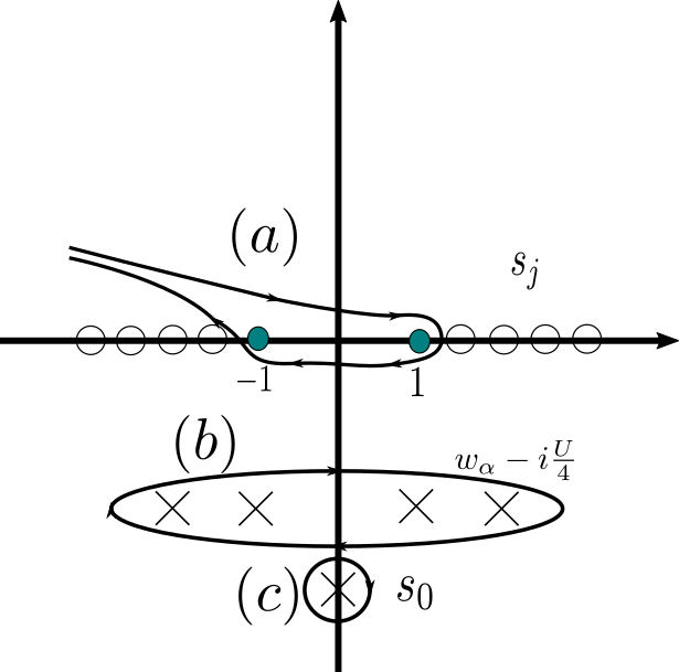
Figure 3: Zeroes and poles of the function $1+\frac{l_{4}}{l_{3}}(t)$: Zeroes (poles) are illustrated by open circles (crosses) and are located at $s_{j}$ ($w_{\alpha}-i\frac{U}{4}$). A pole is located at $s_{0}$ and has order $\frac{N}{2}$. Integration contour with three separate parts: $\left(a\right)$ is starting at $-\infty$, encircling the interval $\left[-1,1\right]$ in clockwise manner and is going back to $-\infty$. $\left(b\right)$ is a loop surrounding all $w_{\alpha}-i\frac{U}{4}$. $\left(c\right)$ is a small circle arround $s_{0}$.

Contour $\left(a\right)$ contains a path $\left(a_{1}\right)$ from $-\infty$ to $-1$, a loop $\left(a_{2}\right)$ around the interval $\left[-1,1\right]$ and a path $\left(a_{3}\right)$ from $-1$ back to $-\infty$. The paths $\left(a_{1}\right)$ and $\left(a_{3}\right)$ are obviously inverse to each other. The integrals on the parts $\left(b\right)$ and $\left(c\right)$ can be calculated. Now we consider $\varSigma_{2}$ and deform the integration contour $\mathcal{L}_{0}$ as above. Note that the integral of $\left.f(t)\right|_{1\text{st branch}}$ on part $\left(a_{2}\right)$ is equal to the integral of $\left.f(t)\right|_{2\text{nd branch}}$ along $\left(a_{2}\right)$ in reversed sense. Now we join the results for $\Sigma_{1}$ and $\Sigma_{2}$ and obtain

$$\varSigma_{1}+\varSigma_{2}=2\pi i\left(\sum_{\alpha=1}^{l}\ln g\left(w_{\alpha}-i\frac{U}{4}\right)+\frac{N}{2}\ln g\left(s_{0}\right)\right)+\intop_{\mathcal{L}}\mathrm{d}t\left.f(t)\right|_{2\text{nd branch}}.$$ (29)

We want to rewrite this result in terms of integrals involving the auxiliary functions (26). To this end we consider

$$\varSigma :=\intop_{\mathcal{L}}\mathrm{d}t\left[\ln g\left(t-i\frac{U}{2}\right)\right]^{\prime}\ln\mathfrak{C}(t)+\intop_{\mathcal{L}}\mathrm{d}t\left[\ln g(t)\right]^{\prime}\ln\frac{1+\mathfrak{\mathfrak{c}+\bar{\mathfrak{c}}}}{\bar{\mathfrak{c}}}(t).$$ (30)

First, we integrate by parts and use that $\ln g\left(t-i\frac{U}{2}\right)$ and $\ln g(t)$ show no jump after surrounding the real axis. Therefore the surface terms vanish. Next we use the factorization

$$\mathfrak{C}(t) =\left(\frac{\sum_{j=1}^{4}l_{j}}{l_{3}+l_{4}}\cdot\frac{l_{3}+l_{4}+\sum_{j=1}^{4}\bar{l}_{j}}{\sum_{j=1}^{4}\left(l_{j}+\bar{l}_{j}\right)}\right)(t),$$

$$\frac{1+\mathfrak{\mathfrak{c}+\bar{\mathfrak{c}}}}{\bar{\mathfrak{c}}}(t) =\frac{\sum_{j=1}^{4}\bar{l}_{j}}{\bar{l}_{3}+\bar{l}_{4}}(t)\cdot\underbrace{\frac{l_{3}+l_{4}+\bar{l}_{1}+\bar{l}_{2}}{l_{3}+l_{4}}(t)}_{=\left.1+\frac{l_{4}}{l_{3}}(t)\right|_{2\text{nd branch}}}$$

and the fact that the second fraction of $\mathfrak{C}(t)$ is analytic along the real axis. According to Cauchy’s theorem it vanishes. Furthermore we deform the integration contour $\mathcal{L}$. This yields a contour with three separate parts, which are illustrated in Fig. 4.

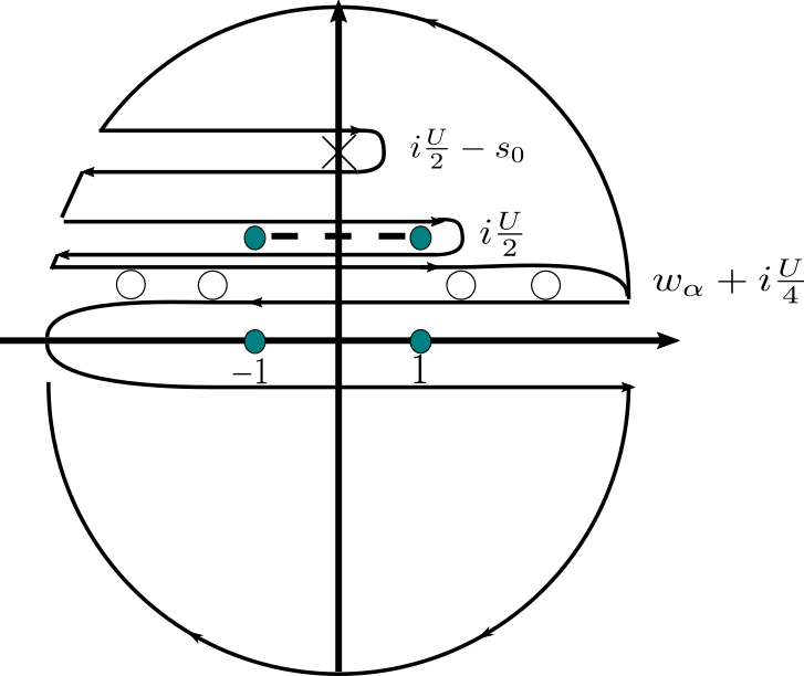
Figure 4: Depiction of zeroes and singularities of $\frac{l_{1}+l_{2}+l_{3}+l_{4}}{l_{3}+l_{4}}(t)$: zeroes are illustrated by open circles, branch cuts by dashed lines and the pole by a cross. We are interested in the integral (30) along the contour $\mathcal{L}$ which runs around the real axis from $\infty+\text{i}\epsilon$ to $-\infty+\text{i}\epsilon$, and then from $-\infty-\text{i}\epsilon$ to $\infty-\text{i}\epsilon$. We add a large semi-circle with radius $R$ to the lower half-plane. The integrand vanishes like $\mathcal{O}\left(\frac{\ln R}{R^{2}}\right)$ asymptotically. Therefore this path does not contribute to the integral (30). Next we add a closed loop that does not encircle any singularities: this consists of a large semi-circle in the upper half-plane and indentations. Finally we drop the loop around the semi-disk in the lower half-plane and the semi-circle in the upper half-plane. This procedure keeps the integral unchanged, but transforms the contour into three indentations. The contours are around the zeroes $w_{\alpha}+i\frac{U}{4}$, the branch cut $\left[-1,1\right]+i\frac{U}{2}$, and the pole $i\frac{U}{2}-s_{0}$ of $\frac{l_{1}+l_{2}+l_{3}+l_{4}}{l_{3}+l_{4}}(t)$ in clockwise manner. The first and third contour integrals can be calculated easily.

The second contour is equal to the contour $\mathcal{L}+i\frac{U}{2}$ in clockwise manner. We rewrite this contour integral by the use of a shift of the integration variable from $t$ to $t+i\frac{U}{2}$. Then we have to exchange $l_{j}(t)$ functions by $\bar{l}_{j}(t)$ functions. Then some integral contributions cancel each other

$$\varSigma =2\pi i\left(\sum_{\alpha=1}^{l}\ln g\left(w_{\alpha}-i\frac{U}{4}\right)-\frac{N}{2}\ln g\left(-s_{0}\right)\right)-\intop_{\mathcal{L}}\mathrm{d}t\ln g(t)\left[\left.\ln\left(1+\frac{l_{4}}{l_{3}}(t)\right)\right|_{2\text{nd branch}}\right]^{\prime}.$$ (31)

Comparing (29) with (31) and using $\left.z(t)\right|_{2\text{nd branch}}=-\frac{1}{\left.z(t)\right|_{1\text{st branch}}}$ yields

$$\varSigma_{1}+\varSigma_{2} =\varSigma+2\pi i\left(\frac{N}{2}\left(\ln g\left(s_{0}\right)+\ln g\left(-s_{0}\right)\right)\right)$$

$$\quad+2\pi i\left[\left(k\circ\ln\left(1+\frac{l_{4}}{l_{3}}\right)\right)(s)+\left(k\circ\ln\left(1+\frac{l_{4}}{l_{3}}\right)\right)\left(s-i\frac{U}{2}\right)\right].$$ (32)

Using

$$\frac{l_{3}+l_{4}+\bar{l}_{1}+\bar{l}_{2}}{l_{3}+l_{4}}(t) =\frac{1+\mathfrak{\mathfrak{c}+\bar{\mathfrak{c}}}}{\bar{\mathfrak{c}}}(t)\frac{\bar{\mathfrak{c}}\mathfrak{B}}{1+\bar{\mathfrak{c}}\mathfrak{B}}(t)$$

we perform the Trotter limit $N\rightarrow\infty$. We drop terms that do not contribute in the limit $N\rightarrow\infty$. Furthermore we also have to drop the term $3N\ln\cos\lambda$ because our $R$-matrix (2) is not normalized as remarked after (2). Instead we have $\check{R}\left(\lambda,0\right)\check{R}\left(0,\lambda\right)=\cos^{6}\lambda,$ which is the term to be dropped. Therefore we find

$$\ln\varLambda^{\text{QTM}}(\lambda) =\left(\frac{1}{2z_{+}(x)}-\frac{z_{-}(x)}{2}-\frac{U}{4}\right)\beta$$

$$\quad+\left(k\circ\ln\frac{1+\mathfrak{\mathfrak{c}+\bar{\mathfrak{c}}}}{1+\bar{\mathfrak{c}}\mathfrak{B}}\right)\left(s\right)+\left(k\circ\ln\frac{\left(1+\mathfrak{c}+\bar{\mathfrak{c}}\right)\bar{\mathfrak{C}}}{\left(1+\bar{\mathfrak{c}}\mathfrak{B}\right)\bar{\mathfrak{c}}}\right)\left(s-i\frac{U}{2}\right)$$

$$\quad+\intop_{\mathcal{L}}\frac{\mathrm{d}t}{2\pi i}\left[\ln g\left(t-i\frac{U}{2}\right)\right]^{\prime}\ln\mathfrak{C}\left(t\right)+\intop_{\mathcal{L}}\frac{\mathrm{d}t}{2\pi i}\left[\ln g\left(t\right)\right]^{\prime}\ln\frac{1+\mathfrak{\mathfrak{c}+\bar{\mathfrak{c}}}}{\bar{\mathfrak{c}}}\left(t\right).$$ (33)

Note that on the right-hand side $x$ and $s=s\left(z_{-}\left(x\right)\right)$ depend on $\lambda$ via (10) and (14) and that $g(t)$ also depends on $x$ (27).

Furthermore note that for $\lambda=0$ the expression for $\ln\varLambda^{\text{QTM}}(\lambda)$ simplifies to the well-known result Jüttner et al. (1998), which yields the host’s contribution to the thermodynamics of our impurity model

$$f_{\text{h}} =-\frac{1}{\beta}\ln\varLambda^{\text{QTM}}\left(0\right),$$ (34)

$$\ln\varLambda^{\text{QTM}}\left(0\right) =-\frac{\beta U}{4}+\intop_{\mathcal{L}}\frac{\mathrm{d}t}{2\pi i}\left[\ln z\left(t-i\frac{U}{2}\right)\right]^{\prime}\ln\mathfrak{C}(t)$$

$$\quad+\intop_{\mathcal{L}}\frac{\mathrm{d}t}{2\pi i}\left[\ln z(t)\right]^{\prime}\ln\frac{1+\mathfrak{c}+\bar{\mathfrak{c}}}{\bar{\mathfrak{c}}}(t).$$ (35)

The impurity contribution to the total free energy $F=L\,f_{h}+f_{i}$ is given by

$$f_{\text{i}} =-\frac{1}{\beta}\ln\varLambda^{\text{QTM}}(\nu),$$ (36)

Equations (26), (33) - (36) completely describe the thermodynamical properties of the Hubbard model with impurity.

For most situations the presented equations need to be treated numerically which is beyond the scope of this paper and will be the topic of a separate publication.

For the so-called half-filled case, however, we are able to perform the low-temperature analysis in Appendix B. There we evaluate the $T^{2}$ contribution of the impurity to the total free energy. The result for the eigenvalue of the impurity transfer matrix is

$$\ln\varLambda^{\text{QTM}}\left(\lambda\right)= -\frac{U\beta}{4}+\beta\intop_{-1}^{1}\frac{\mathrm{d}t}{2\pi\text{i}}\left[\ln\frac{g\left(t\right)}{\bar{g}\left(t\right)}\right]^{\prime}\left(\kappa\ast f\right)(t)$$

$$+\frac{U}{12\beta}\frac{1}{J_{0}\left({2\pi i}/U\right)+J_{2}\left({2\pi i}/U\right)}\sum_{n=0}^{\infty}J_{2n}\left(\frac{2\pi i}{U}\right)z_{-}^{-2n}\left(\lambda\right),$$ (37)

where $z_{-}(\lambda)$ is defined in (7). Here and in the remainder of the paper, $\ast$ denotes the convolution of two functions $\left(f\ast g\right)(x)=\frac{1}{2\pi}\int dyf(x-y)g(y)$. Note that $z_{-}(\lambda)\to\infty$ for $\lambda\to 0$ in which case only the $n=0$ term in the series contributes. The third term in expression (37) is real. The functions $\kappa\left(t\right)$ and $f\left(t\right)$ are even functions and thus $\left(\kappa\ast f\right)(t)$ is also even. Examination of the ratio $\gamma(t):={g(t)}/{\bar{g}(t)}$ for $z_{\pm}\left(\nu\right)\in\mathbb{R}$ shows that $\gamma(t)/\gamma(-t)$ is unimodular, and hence $(\ln\gamma)^{\prime}(t)+(\ln\gamma)^{\prime}(-t)$ is purely imaginary. This renders the second term on the r.h.s. of equation (37) real.

We would like to note that it is possible to find alternative expressions for $\ln\varLambda^{\text{QTM}}(\lambda)$. These alternative expressions are based on the thermodynamic Bethe ansatz (TBA) and are given in Appendix C.

IV Conclusion

We constructed a Hubbard model with integrable impurity and derived the Bethe ansatz equations for the Hamiltonian. The impurity leads to an additional phase factor in the first set of the nested Bethe ansatz equations of the row-to-row transfer matrix resp. the Hamiltonian. For the finite temperature properties, two sets of non-linear integral equations were derived: The infinitely many thermodynamic Bethe ansatz equations and the finitely many non-linear integral equations in the quantum transfer matrix approach. In both cases the actual integral equations are unmodified by the impurity, i.e. they are identical to those of the homogeneous chain. The impurity appears in new integral expressions of the thermodynamical potential which for the impurity are different from those for the host.

Within the framework of TBA we used the string hypothesis for the new Bethe ansatz equations of the Hamiltonian and followed the traditional procedure Takahashi (1972). Here, the derivation of the expression for the impurity contribution to the thermodynamical potential was relatively straightforward. The complexity of the infinitely many TBA equations, however, constrains the practical use of this expression.

The derivation of the impurity contribution in terms of the finitely many auxiliary functions that appear in the quantum transfer matrix approach Jüttner et al. (1998) was much more involved. It filled a substantial part of this paper and constitutes the major result which allows for practical calculations. As an example of such calculations we calculated the low-temperature asymptotics in the case of half filling. We are convinced that these results realize a significant extension of the established knowledge of the Hubbard model Essler et al. (2005).

The Hubbard chain with integrable impurity is interesting in its own right. In this present work, the foundation was laid for the investigation of the finite-temperature behavior by numerically solving the finitely many non-linear integral equations. A truncation like for the TBA equations presented in the Appendix is not necessary. We can now evaluate the specific heat and entropy numerically. At high temperature $T$ the impurity spin will decouple from the host, but at low temperatures $T$ the impurity spin will be screened. The resulting Kondo physics will depend on the system parameters. Another application of the presented work are chains with more than one impurity site. The behavior of this type of impurities is special, since the scattering of particles on the two impurities at positions $j$ and $k$ does not depend on the difference $j-k$. This follows obviously from the construction of the commuting family of transfer matrices.

Beyond this, the integrable Hubbard chain with impurity also allows for new studies of the Anderson impurity model. In a future publication we will present a suitable continuum limit of the Hubbard model leading to a non-interacting host that interacts with an impurity with spin and charge degrees of freedom. In this way we will derive a new set of finitely many non-linear integral equations for the celebrated integrable Anderson impurity model.

V Appendix A - Expressions for the Hamiltonian

We find

$$R_{jk}\left(\nu,0\right)= e^{2h\left(\nu\right)}+e^{h\left(\nu\right)}\left(\cos^{-1}\nu-e^{h\left(\nu\right)}\right)\sum_{\sigma=\uparrow,\downarrow}\left(n_{j\sigma}+n_{k\sigma}\right)$$

$$+e^{h\left(\nu\right)}\left(e^{h\left(\nu\right)}-\frac{2}{\cos\nu}+\frac{e^{h\left(\nu\right)}}{\cos^{2}\nu}\right)\left(n_{j\uparrow}n_{j\downarrow}+n_{k\uparrow}n_{k\downarrow}\right)$$

$$+\left(e^{2h\left(\nu\right)}+\cos^{-2}\nu\right)\left(n_{j\uparrow}n_{k\downarrow}+n_{j\downarrow}n_{k\uparrow}\right)$$

$$+\left(1+e^{2h\left(\nu\right)}\right)\sum_{\sigma=\uparrow,\downarrow}n_{j\sigma}n_{k\sigma}+\left(1-e^{2h\left(\nu\right)}\right)\left(1+\cos^{-2}\nu\right)\sum_{\sigma=\uparrow,\downarrow}n_{j\sigma}n_{k\uparrow}n_{k\downarrow}$$

$$+\left(\frac{4e^{h\left(\nu\right)}}{\cos\nu}-\frac{1+e^{2h\left(\nu\right)}}{\cos^{2}\nu}-1-e^{2h\left(\nu\right)}\right)n_{j\uparrow}n_{j\downarrow}\left(\sum_{\sigma=\uparrow,\downarrow}n_{k\sigma}-2n_{k\uparrow}n_{k\downarrow}\right)$$

$$+\tan\nu\sum_{\sigma=\uparrow,\downarrow}\left(c_{j\sigma}c_{k\sigma}^{\dagger}-e^{2h\left(\nu\right)}c_{j\sigma}^{\dagger}c_{k\sigma}\right)$$

$$+e^{h\left(\nu\right)}\tan\nu\left(e^{h\left(\nu\right)}-\cos^{-1}\nu\right)\left(c_{j\uparrow}^{\dagger}n_{j\downarrow}c_{k\uparrow}+n_{j\uparrow}c_{j\downarrow}^{\dagger}c_{k\downarrow}+c_{j\uparrow}^{\dagger}c_{k\uparrow}n_{k\downarrow}+c_{j\downarrow}^{\dagger}n_{k\uparrow}c_{k\downarrow}\right)$$

$$+\tan\nu\left(\frac{e^{h\left(\nu\right)}}{\cos\nu}-1\right)\left(c_{j\uparrow}n_{j\downarrow}c_{k\uparrow}^{\dagger}+n_{j\uparrow}c_{j\downarrow}c_{k\downarrow}^{\dagger}+c_{j\uparrow}c_{k\uparrow}^{\dagger}n_{k\downarrow}+c_{j\downarrow}n_{k\uparrow}c_{k\downarrow}^{\dagger}\right)$$

$$+\tan\nu\left(\frac{2e^{h\left(\nu\right)}}{\cos\nu}-1-e^{2h\left(\nu\right)}\right)\left(c_{j\uparrow}^{\dagger}n_{j\downarrow}c_{k\uparrow}n_{k\downarrow}+n_{j\uparrow}c_{j\downarrow}^{\dagger}n_{k\uparrow}c_{k\downarrow}-c_{j\uparrow}n_{j\downarrow}c_{k\uparrow}^{\dagger}n_{k\downarrow}\right.$$

$$\hphantom{+\tan\nu\left(\frac{2e^{h\left(\nu\right)}}{\cos\nu}-1-e^{2h\left(\nu\right)}\right)\left(\right.\,}\left.-n_{j\uparrow}c_{j\downarrow}n_{k\uparrow}c_{k\downarrow}^{\dagger}\right)$$

$$+\tan^{2}\nu\left(c_{j\uparrow}^{\dagger}c_{j\downarrow}c_{k\uparrow}c_{k\downarrow}^{\dagger}+c_{j\uparrow}c_{j\downarrow}^{\dagger}c_{k\uparrow}^{\dagger}c_{k\downarrow}-e^{2h\left(\nu\right)}\left(c_{j\uparrow}^{\dagger}c_{j\downarrow}^{\dagger}c_{k\uparrow}c_{k\downarrow}+c_{j\uparrow}c_{j\downarrow}c_{k\uparrow}^{\dagger}c_{k\downarrow}^{\dagger}\right)\right).$$

Note that $R_{jk}\left(0,\nu\right)$ has a similar form

$$R_{jk}\left(0,\nu\right)= e^{-2h\left(\nu\right)}+e^{-h\left(\nu\right)}\left(\cos^{-1}\nu-e^{-h\left(\nu\right)}\right)\sum_{\sigma=\uparrow,\downarrow}\left(n_{j\sigma}+n_{k\sigma}\right)$$

$$+e^{-h\left(\nu\right)}\left(e^{-h\left(\nu\right)}-\frac{2}{\cos\nu}+\frac{e^{-h\left(\nu\right)}}{\cos^{2}\nu}\right)\left(n_{j\uparrow}n_{j\downarrow}+n_{k\uparrow}n_{k\downarrow}\right)$$

$$+\left(e^{-2h\left(\nu\right)}+\cos^{-2}\nu\right)\left(n_{j\uparrow}n_{k\downarrow}+n_{j\downarrow}n_{k\uparrow}\right)$$

$$+\left(1+e^{-2h\left(\nu\right)}\right)\sum_{\sigma=\uparrow,\downarrow}n_{j\sigma}n_{k\sigma}+\left(1-e^{-2h\left(\nu\right)}\right)\left(1+\cos^{-2}\nu\right)\sum_{\sigma=\uparrow,\downarrow}n_{j\sigma}n_{k\uparrow}n_{k\downarrow}$$

$$+\left(\frac{4e^{-h\left(\nu\right)}}{\cos\nu}-\frac{1+e^{-2h\left(\nu\right)}}{\cos^{2}\nu}-1-e^{-2h\left(\nu\right)}\right)n_{j\uparrow}n_{j\downarrow}\left(\sum_{\sigma=\uparrow,\downarrow}n_{k\sigma}-2n_{k\uparrow}n_{k\downarrow}\right)$$

$$+\tan\nu\sum_{\sigma=\uparrow,\downarrow}\left(c_{j\sigma}^{\dagger}c_{k\sigma}-e^{-2h\left(\nu\right)}c_{j\sigma}c_{k\sigma}^{\dagger}\right)$$

$$+e^{-h\left(\nu\right)}\tan\nu\left(e^{-h\left(\nu\right)}-\cos^{-1}\nu\right)\left(c_{j\uparrow}n_{j\downarrow}c_{k\uparrow}^{\dagger}+n_{j\uparrow}c_{j\downarrow}c_{k\downarrow}^{\dagger}+c_{j\uparrow}c_{k\uparrow}^{\dagger}n_{k\downarrow}+c_{j\downarrow}n_{k\uparrow}c_{k\downarrow}^{\dagger}\right)$$

$$+\tan\nu\left(\frac{e^{-h\left(\nu\right)}}{\cos\nu}-1\right)\left(c_{j\uparrow}^{\dagger}n_{j\downarrow}c_{k\uparrow}+n_{j\uparrow}c_{j\downarrow}^{\dagger}c_{k\downarrow}+c_{j\uparrow}^{\dagger}c_{k\uparrow}n_{k\downarrow}+c_{j\downarrow}^{\dagger}n_{k\uparrow}c_{k\downarrow}\right)$$

$$+\tan\nu\left(1+e^{-2h\left(\nu\right)}-\frac{2e^{-h\left(\nu\right)}}{\cos\nu}\right)\left(c_{j\uparrow}^{\dagger}n_{j\downarrow}c_{k\uparrow}n_{k\downarrow}+n_{j\uparrow}c_{j\downarrow}^{\dagger}n_{k\uparrow}c_{k\downarrow}-c_{j\uparrow}n_{j\downarrow}c_{k\uparrow}^{\dagger}n_{k\downarrow}\right.$$

$$\hphantom{+\tan\nu\left(1+e^{-2h\left(\nu\right)}-\frac{2e^{-h\left(\nu\right)}}{\cos\nu}\right)\left(\right.\,}\left.-n_{j\uparrow}c_{j\downarrow}n_{k\uparrow}c_{k\downarrow}^{\dagger}\right)$$

$$+\tan^{2}\nu\left(c_{j\uparrow}^{\dagger}c_{j\downarrow}c_{k\uparrow}c_{k\downarrow}^{\dagger}+c_{j\uparrow}c_{j\downarrow}^{\dagger}c_{k\uparrow}^{\dagger}c_{k\downarrow}-e^{-2h\left(\nu\right)}\left(c_{j\uparrow}^{\dagger}c_{j\downarrow}^{\dagger}c_{k\uparrow}c_{k\downarrow}+c_{j\uparrow}c_{j\downarrow}c_{k\uparrow}^{\dagger}c_{k\downarrow}^{\dagger}\right)\right).$$

These formulas can be used in equation (5) and (6). The impurity part of the Hamiltonian has the form

$$h_{\text{imp}}=\alpha_{0}\left(\nu,U\right)\left(h_{l,i}+h_{i,r}\right)+\alpha_{2}\left(\nu,U\right)h_{l,r}+\alpha_{1}\left(\nu,U\right)\left[\left(h_{l,i}+h_{i,r}\right),h_{l,r}\right],$$

where the prefactors $\alpha_{j}\left(\nu,U\right)$, $j=0,1,2$ are quite bulky expressions in terms of the model parameters. However, $\alpha_{0}$ and $\alpha_{2}$ are real, and $\alpha_{1}$ is imaginary for real $\nu$. Hence, $h_{\text{imp}}$ is hermitian.

VI Appendix B - Half filling Case for low temperatures

In the following we analyze the behavior of our model in the case of half filling and low temperatures. In this case $\mathfrak{c}\left(t\right)$ and $\mathfrak{\bar{c}}\left(t\right)$ in equations (26) are obviously small. Hence, terms like $\ln\left(1+\mathfrak{c}\left(t\right)\right)$ or $\ln\left(1+\mathfrak{\bar{c}\left(t\right)}\right)$ may be dropped, but not $\ln\bar{\mathfrak{c}}\left(t\right)$.

The equations simplify by use of the definitions $a\left(t\right)=\mathfrak{b}\left(t-\text{i}\frac{U}{4}\right)$ and $\bar{a}\left(t\right)=\mathfrak{b}^{-1}\left(t+\text{i}\frac{U}{4}\right)$ as well as reducing the contour integrals to integrals on the real axis. Using the Fourier transformation we find in $k$-space

$$\mathfrak{a}\left(k\right) =-\frac{e^{-\frac{U}{4}\left(\left|k\right|-2k\right)}}{1+e^{-\frac{U}{2}\left|k\right|}}\beta\mathfrak{f}\left(k\right)+\frac{e^{-\frac{U}{2}\left|k\right|}}{1+e^{-\frac{U}{2}\left|k\right|}}\mathfrak{A}\left(k\right)-\frac{e^{-\frac{U}{2}\left(\left|k\right|+k\right)}}{1+e^{-\frac{U}{2}\left|k\right|}}\bar{\mathfrak{A}}\left(k\right),$$

$$\bar{\mathfrak{a}}\left(k\right) =-\frac{e^{-\frac{U}{4}\left|k\right|}}{1+e^{-\frac{U}{2}\left|k\right|}}\beta\mathfrak{f}\left(k\right)+\frac{e^{-\frac{U}{2}\left|k\right|}}{1+e^{-\frac{U}{2}\left|k\right|}}\bar{\mathfrak{A}}\left(k\right)-\frac{e^{-\frac{U}{2}\left(\left|k\right|+k\right)}}{1+e^{-\frac{U}{2}\left|k\right|}}\mathfrak{A}\left(k\right),$$ (38)

where $\mathfrak{a}\left(k\right)=\mathcal{F}\left\{\ln a\right\}\left(k\right)$, $\bar{\mathfrak{a}}\left(k\right)=\mathcal{F}\left\{\ln\bar{a}\right\}\left(k\right)$, $\mathfrak{A}\left(k\right)=\mathcal{F}\left\{\ln\left(1+a\right)\right\}\left(k\right)$, $\bar{\mathfrak{A}}\left(k\right)=\mathcal{F}\left\{\ln\left(1+\bar{a}\right)\right\}\left(k\right)$ and

$$\mathfrak{f}\left(k\right)={4\pi}\frac{J_{1}\left(k\right)}{k}=2\pi\left[J_{0}\left(k\right)+J_{2}\left(k\right)\right].$$ (39)

Note that $\mathfrak{f}\left(k\right)$ is the Fourier transform of

$$f\left(t\right)=4\sqrt{1-t^{2}}\Theta\left(1-t^{2}\right)=\intop_{\mathbb{R}}\frac{\mathrm{d}k}{2\pi}e^{\text{i}kt}\mathfrak{f}\left(k\right).$$

The Fourier transform of (38) is

$$\ln a =-\beta e\ast f+\kappa\ast\ln A-\kappa_{-}\ast\ln\bar{A},$$

$$\ln\bar{a} =-\beta e\ast f+\kappa\ast\ln\bar{A}-\kappa_{+}\ast\ln A,$$ (40)

where the functions $e(x)$ and $\kappa(x)$ are defined by

$$e(x)=\frac{1}{U}\frac{1}{\cosh\frac{2\pi x}{U}},\quad\kappa(x)=\intop_{\mathbb{R}}\frac{\mathrm{d}k}{2\pi}e^{\text{i}kx}\frac{e^{-\frac{U}{2}\left|k\right|}}{1+e^{-\frac{U}{2}\left|k\right|}}$$ (41)

and $\kappa_{\pm}(x)=\kappa(x\pm i{U}/{2})$.

The driving term in (40) has exponential asymptotics

$$e\ast f(x)\simeq\frac{2}{U}\mathfrak{f}\left(\frac{2\pi i}{U}\right)\exp\left(-\frac{2\pi\left|x\right|}{U}\right),\qquad(|x|\to\infty).$$ (42)

By use of the dilog-trick we obtain in the low-temperature limit $(\beta\to\infty)$

$$\intop_{0(-\infty)}^{\infty(0)}\mathrm{d}x\exp\left(-\frac{2\pi\left|x\right|}{U}\right)\ln\left(A(x)\bar{A}(x)\right)\simeq\frac{\pi U^{2}}{24\beta\mathfrak{f}\left({2\pi i}/U\right)}.$$ (43)

Performing the same analysis for the free energy (33) leads to a significant simplification. Again, $\ln\bar{\mathfrak{c}}\left(t\right)$ must be treated carefully. All explicit terms simplify to the constant $-\frac{U\beta}{4}$. Almost all integral expressions disappear. The only term left comes from the last integral expression in equation (33)

$$\ln\varLambda^{\text{QTM}}\left(\lambda\right)=-\frac{U\beta}{4}-\intop_{-1}^{1}\frac{\mathrm{d}t}{2\pi\text{i}}\left[\ln\frac{g\left(t\right)}{\bar{g}\left(t\right)}\right]^{\prime}\left(\hat{K}_{1}\oblong\ln\mathfrak{B}\right)(t),$$

where $\bar{g}\left(t\right)$ is the function $g\left(t\right)$ on the second sheet. Rewriting this expression in the functions $a\left(t\right)$ and $\bar{a}\left(t\right)$ yields

$$\ln\varLambda^{\text{QTM}}\left(\lambda\right)=-\frac{U\beta}{4}+\intop_{-1}^{1}\frac{\mathrm{d}t}{2\pi\text{i}}\left[\ln\frac{g\left(t\right)}{\bar{g}\left(t\right)}\right]^{\prime}\left(\beta\left(\kappa\ast f\right)(t)+\left(e\ast\ln\left(A\bar{A}\right)\right)\left(t\right)\right).$$ (44)

We want to evaluate the $\beta^{-1}$ contribution to this integral. It is given by the $e\ast\ln\left(A\bar{A}\right)$ term which has low-temperature asymptotics

$$\left(e\ast\ln\left(A\bar{A}\right)\right)\left(t\right)\simeq\frac{\pi U}{6\beta\mathfrak{f}\left({2\pi i}/U\right)}\cosh\frac{2\pi t}{U}.$$ (45)

By use of the generating function of Bessel’s functions we carry out the integral and obtain (37).

VII Appendix C - TBA

In this appendix we apply alternatively to the main body of the paper the thermodynamic Bethe ansatz (TBA). For the Hubbard model with impurity site we will see that the non-linear integral equations Takahashi (1972) as obtained for the pure Hubbard model (1) still hold as well as the integral expression for the host’s contribution to the thermodynamical potential. However, a new integral expression for the impurity’s contribution appears.

We use the string hypothesis Takahashi (1972); Essler et al. (2005) according to which all finite solutions of $\left\{k_{j}\right\}_{j=1}^{K}$ and $\left\{\varLambda_{l}\right\}_{l=1}^{M}$ of (8) are composed of three different classes of strings

• a single real momentum $k_{j}$,

• $m$ $\varLambda$’s combining into a $\varLambda$ string,

• $2m$ $k$’s and $m$ $\varLambda$’s combining into a $k$-$\varLambda$ string.

For large lattices ($L\gg 1$) and a large number of electrons ($K\gg 1$), nearly for all strings the imaginary parts of the $k$’s and $\varLambda$’s are evenly spaced.

Solving the equations (8) is simplified by use of the string hypothesis. For arbitrary values of $K$ electrons and $M$ down spins any solution of (8) is described by a distribution of strings with $M_{n}$ $\varLambda$-strings and $M_{n}^{\prime}$ $k$-$\varLambda$ strings of length $n$ ($n=1,2,\ldots$) and $\mathcal{M}_{e}$ single $k_{j}$’s. The numbers $\mathcal{M}_{e}$, $M_{n}$ and $M_{n}^{\prime}$ are occupation numbers of the string configuration and satisfy the sum rules

$$M =\sum_{n=1}^{\infty}n\left(M_{n}+M_{n}^{\prime}\right),$$

$$K =\mathcal{M}_{e}+\sum_{n=1}^{\infty}2nM_{n}^{\prime}.$$

Subjecting the string distribution to equations (8) and using

$$e^{i\hat{\delta}\left(k_{j}\right)}:=\text{e}^{2h(\nu)}\frac{\text{e}^{\text{i}k_{j}}/{z_{+}(\nu)}+1}{z_{-}(\nu)-\text{e}^{\text{i}k_{j}}}$$

we find for even $L$ in logarithmic form Takahashi’s equations for the purely real centers of the strings. In the thermodynamical limit $L\rightarrow\infty,$ $\frac{K}{L}$ and $\frac{M}{L}$ fixed, solutions of Takahashi’s equations should be expressed in terms of distributions of particles $\rho^{p}\left(k\right)$, $\sigma_{n}^{p}\left(\varLambda\right)$, $\sigma_{n}^{\prime p}\left(\varLambda\right)$ and the appropriate $\rho^{h}\left(k\right),\sigma_{n}^{h}\left(\varLambda\right),\sigma_{n}^{\prime h}\left(\varLambda\right)$. In the thermodynamic limit Takahashi’s equations can be expressed as coupled integral equations involving the root densities Takahashi (1972); Essler et al. (2005) for particles and holes

$$\rho^{p}\left(k\right)+\rho^{h}\left(k\right) =\frac{1}{2\pi}+\frac{\hat{\Delta}\left(k\right)}{L}+\cos k\sum_{n=1}^{\infty}\intop_{-\infty}^{\infty}\mathrm{d}\varLambda a_{n}\left(\varLambda-\sin k\right)\left(\sigma_{n}^{\prime p}\left(\varLambda\right)+\sigma_{n}^{p}\left(\varLambda\right)\right),$$

$$\sigma_{n}^{h}\left(\varLambda\right) =-\sum_{m=1}^{\infty}\left.A_{nm}\ast\sigma_{m}^{p}\right|_{\varLambda}+\intop_{-\pi}^{\pi}\mathrm{d}ka_{n}\left(\varLambda-\sin k\right)\rho^{p}\left(k\right),$$

$$\sigma_{n}^{\prime h}\left(\varLambda\right) =\frac{1}{\pi}\text{Re}\frac{1}{\sqrt{1-\left(\varLambda-ni\frac{U}{4}\right)^{2}}}+\frac{2}{\pi L}\partial_{\varLambda}\hat{\delta}\left(\text{Re}\sqrt{1-\left(\varLambda-ni\frac{U}{4}\right)^{2}}\right)$$

$$\quad-\sum_{m=1}^{\infty}\left.A_{nm}\ast\sigma_{m}^{\prime p}\right|_{\varLambda}-\intop_{-\pi}^{\pi}\mathrm{d}ka_{n}\left(\sin k-\varLambda\right)\rho^{p}\left(k\right),$$ (46)

where $\hat{\Delta}\left(k\right)=\frac{1}{2\pi}\partial_{k}\hat{\delta}\left(k\right),$ $a_{n}\left(x\right)$ is a shorthand notation for

$$a_{n}\left(x\right)=\frac{1}{2\pi}\frac{n\frac{U}{2}}{\left(n\frac{U}{4}\right)^{2}+x^{2}},$$

and $A_{nm}*$ is an integral operator that acts on a function $f\left(x\right)$ as

$$\left.A_{nm}\ast f\right|_{x}=\delta_{nm}f\left(x\right)+\intop_{-\infty}^{\infty}\frac{\mathrm{d}y}{2\pi}\frac{\mathrm{d}}{\mathrm{d}x}\varTheta_{nm}\left(\frac{x-y}{U/4}\right)f\left(y\right).$$

Note that in general $\ast$ denotes the convolution of two functions. The ad hoc definition of $A_{nm}*$ avoids the introduction of a function $A_{nm}$ with delta function contribution.

For further transformations of (46) the following relation is of great use

$$\intop_{-\pi}^{\pi}\frac{\mathrm{d}k}{2}a_{n}\left(\varLambda-\sin k\right)=\text{Re}\frac{1}{\sqrt{1-\left(\varLambda-ni\frac{U}{4}\right)^{2}}}.$$

To find the state of thermodynamic equilibrium we locate, following the principles of statistical mechanics, the minimum of the thermodynamical potential Tsvelick and Wiegmann (1983) per site

$$f=e-\mu n_{c}-2Bm-Ts.$$

where $\mu$ is the chemical potential, $B$ the magnetic field, $T$ the temperature, $n_{c}$ the particle density, $m$ the magnetization and $s$ is the total entropy per site. We restrict ourselves to a magnetic field $B\geq 0$ and to a chemical potential $\mu\leq 0$.

In the thermodynamic limit, we use the root densities of particles and holes and consider the entropy as a functional in terms of the root densities.

We use Stirling’s formula to approximate the factorials in the contribution $\mathrm{d}S$ to the entropy, since the logarithm of the number of states is large in the thermodynamic limit. The thermodynamical potential per site $f$ is a functional in terms of the root densities. With respect to variations in a maximal set of independent root densities the state of thermodynamic equilibrium must be a stationary point. Equations (46) give the densities of holes in terms of the densities of particles. Hence the variational condition $\delta f=0$ is to be solved under the constraint equations (46). This results into the thermodynamical Bethe ansatz equations just for the ratios

$$\zeta\left(k\right)=\frac{\rho^{h}\left(k\right)}{\rho^{p}\left(k\right)},\qquad\eta_{n}\left(\varLambda\right)=\frac{\sigma_{n}^{h}\left(\varLambda\right)}{\sigma_{n}^{p}\left(\varLambda\right)},\qquad\eta_{n}^{\prime}\left(\varLambda\right)=\frac{\sigma_{n}^{\prime h}\left(\varLambda\right)}{\sigma_{n}^{\prime p}\left(\varLambda\right)},$$

and as mentioned already above are identical to those of the pure Hubbard model Takahashi (1972)

$$\ln\zeta\left(k\right) =-\frac{2\cos k}{T}-\frac{4}{T}\intop_{-\infty}^{\infty}\mathrm{d}y\,s(\sin k-y)\text{Re}\sqrt{1-\left(y-i\frac{U}{4}\right)^{2}}+\left(s\ast\ln\frac{1+\eta_{1}^{\prime}}{1+\eta_{1}}\right)\left(\sin k\right),$$

$$\eta_{0}\left(\varLambda\right) =\eta_{0}^{\prime}\left(\varLambda\right)=0,$$

$$\ln\eta_{n}\left(\varLambda\right) =\left(s\ast\ln\left(\left(1+\eta_{n-1}\right)\left(1+\eta_{n+1}\right)\right)\right)\left(\varLambda\right)-\delta_{1n}\left(s\ast\ln\left(1+\zeta^{-1}\right)\right)\left(\varLambda\right),$$

$$\ln\eta_{n}^{\prime}\left(\varLambda\right) =\left(s\ast\ln\left(\left(1+\eta_{n-1}\right)\left(1+\eta_{n+1}\right)\right)\right)\left(\varLambda\right)-\delta_{1n}\left(s\ast\ln\left(1+\zeta\right)\right)\left(\varLambda\right),$$ (47)

for $n=1,2,\ldots$ and with integral kernel $s\left(x\right)=\frac{1}{U\text{ch}\frac{2\pi x}{U}}$ in the convolutions. Equations (47) are completed by the boundary conditions

$$\lim_{n\rightarrow\infty}\frac{\ln\eta_{n}}{n}=\frac{2B}{T},\qquad\lim_{n\rightarrow\infty}\frac{\ln\eta_{n}^{\prime}}{n}=-\frac{2\mu}{T}.$$

The thermodynamical potential per site of the host is given in terms of solutions to (47) as

$$f_{\text{h}} =\frac{U}{4}-T\intop_{-\pi}^{\pi}\frac{\mathrm{d}k}{2\pi}\ln\left(1+\zeta^{-1}\left(k\right)\right)$$

$$\quad-T\sum_{n=1}^{\infty}\intop_{-\infty}^{\infty}\frac{\mathrm{d}\varLambda}{\pi}\ln\left(1+\left(\eta_{n}^{\prime}\right)^{-1}\left(\varLambda\right)\right)\text{Re}\frac{1}{\sqrt{1-\left(\varLambda-in\frac{U}{4}\right)^{2}}}.$$ (48)

The total thermodynamical potential is of the form

$$F=Lf_{\text{h}}+f_{\text{i}},$$ (49)

where $f_{\text{i}}$ is the impurity part of the thermodynamical potential

$$f_{\text{i}} =\frac{U}{4}-T\intop_{-\pi}^{\pi}\mathrm{d}k\hat{\Delta}\left(k\right)\ln\left(1+\zeta^{-1}\left(k\right)\right)$$

$$\quad-T\sum_{n=1}^{\infty}\intop_{-\pi}^{\pi}\mathrm{d}k\intop_{-\infty}^{\infty}\mathrm{d}\varLambda\hat{\Delta}\left(k\right)a_{n}\left(\varLambda-\sin k\right)\ln\left(1+\left(\eta_{n}^{\prime}\right)^{-1}\left(\varLambda\right)\right).$$ (50)

Equations (47), (48), (50) and (49) completely describe the thermodynamical properties of the Hubbard model with impurity. The equivalence of the thermodynamical equations was shown in Cavaglià et al. (2015). Note that for $z_{\pm}\left(\nu\right)\in\mathbb{R}$ (that is, for example, for $\nu\in\mathbb{R}$), expression (50) yields a real result: The odd part $\hat{\delta}\left(k\right)-\hat{\delta}\left(-k\right)$ of the function $\hat{\delta}\left(k\right)$ is real, hence $\hat{\Delta}\left(k\right)+\hat{\Delta}\left(-k\right)$ is real too and all other factors in (50) are even in $k$. Therefore the result of (50) is real.

VIII Acknowledgment

YÖ is grateful to Studienstiftung des deutschen Volkes (German Academic Scholarship Foundation) for a PhD grant. Both authors acknowledge financial support by Deutsche Forschungsgemeinschaft within FOR 2316 ”Correlations in Integrable Quantum Many-Body Systems”.

References

• Lieb and Wu (1968) E. H. Lieb and F. Y. Wu, Physical Review Letters 20, 1445 (1968).
• Essler and Korepin (1994a) F. H. L. Essler and V. E. Korepin, Physical Review Letters 72, 908 (1994a).
• Essler and Korepin (1994b) F. H. L. Essler and V. E. Korepin, Nuclear Physics B 426, 505 (1994b).
• Shastry (1986a) B. S. Shastry, Physical Review Letters 56, 2453 (1986a).
• Ramos and Martins (1997) P. B. Ramos and M. J. Martins, Journal of Physics A: Mathematical and General 30, L195 (1997).
• Martins and Ramos (1998) M. J. Martins and P. B. Ramos, Nuclear Physics B 522, 413 (1998).
• Takahashi (1972) M. Takahashi, Progress of Theoretical Physics 47, 69 (1972).
• Takahashi (1974) M. Takahashi, Progress of Theoretical Physics 52, 103 (1974).
• Kawakami et al. (1989) N. Kawakami, T. Usuki,  and A. Okiji, Physics Letters A 137, 287 (1989).
• Usuki et al. (1990) T. Usuki, N. Kawakami,  and A. Okiji, Journal of Physical Society of Japan 59, 1357 (1990).
• Deguchi et al. (2000) T. Deguchi, F. H. L. Essler, F. Göhmann, A. Klümper, V. E. Korepin,  and K. Kusakabe, Physics Reports 331, 197 (2000).
• Essler et al. (2005) F. H. L. Essler, H. Frahm, F. Göhmann, A. Klümper,  and V. E. Korepin, The One-Dimensional Hubbard Model (Cambridge University Press, Cambridge, 2005).
• Shastry (1986b) B. S. Shastry, Physical Review Letters 56, 1529 (1986b).
• Shiroishi and Wadati (1995) M. Shiroishi and M. Wadati, Journal of the Physical Society of Japan 64, 57 (1995).
• Andrei (1995) N. Andrei, Series in Modern Condensed Matter Physics 6, 457 (1995).
• Yue and Deguchi (1997) R. Yue and T. Deguchi, Journal of Physics A: Mathematical and General 30, 849 (1997).
• Jüttner et al. (1998) G. Jüttner, A. Klümper,  and J. Suzuki, Nuclear Physics B 522, 471 (1998).
• Tsunetsugu (1991) H. Tsunetsugu, Journal of the Physical Society of Japan 60, 1460 (1991).
• Umeno et al. (2003) Y. Umeno, M. Shiroishi,  and A. Klümper, Europhysics Letters 62, 384 (2003).
• Cavaglià et al. (2015) A. Cavaglià, M. Cornagliotto, M. Mattelliano,  and R. Tateo, Journal of High Energy Physics 06, 015 (2015).
• Andrei and Johannesson (1984) N. Andrei and H. Johannesson, Physics Letters A 100, 108 (1984).
• Zvyagin and Schlottmann (1997) A. A. Zvyagin and P. Schlottmann, Physical Review B 56, 300 (1997).
• Shastry (1988) B. S. Shastry, Journal of Statistical Physics 50, 57 (1988).
• Tsvelick and Wiegmann (1983) A. M. Tsvelick and P. B. Wiegmann, Advances in Physics 32, 453 (1983).