The Luttinger-Kohn theory for multiband Hamiltonians: A revision of ellipticity requirements

Abstract

Modern applications require a robust and theoretically solid tool for the realistic modeling of electronic states in low dimensional nanostructures. The $k\cdot p$ theory has fruitfully served this role for the long time since its establishment. During the last three decades several problems have been detected in connection with the application of the $k\cdot p$ approach to such nanostructures. These problems are closely related to the violation of the ellipticity conditions for the underlying model, the fact that has been largely overlooked in the literature. We derive ellipticity conditions for $6\times 6$, $8\times 8$ and $14\times 14$ Hamiltonians obtained by the application of Luttinger-Kohn theory to the bulk zinc blende (ZB) crystals, and demonstrate that the corresponding models are non-elliptic for many common crystalline materials. With the aim to obtain the admissible (in terms of ellipticity) parameters, we further develop and justify a parameter rescaling procedure for $8\times 8$ Hamiltonians. This allows us to calculate the admissible parameter sets for GaAs, AlAs, InAs, GaP, AlP, InP, GaSb, AlSb, InSb, GaN, AlN, InN. The newly obtained parameters are then optimized in terms of the bandstructure fit by changing the value of the inversion asymmetry parameter $B$ that is proved to be essential for ellipticity of $8\times 8$ Hamiltonian. The consecutive analysis, performed here for all mentioned $k\cdot p$ Hamiltonians, indicates the connection between the lack of ellipticity and perturbative terms describing the influence of out-of-basis bands on the structure of the Hamiltonian. This enables us to quantify the limits of models’ applicability material-wise and to suggest a possible unification of two different $14\times 14$ models, analysed in this work.

I Introduction

The collection of methods known as an effective mass theory is one of the fundamental topics in the physics of nanostructures. The theory has been used to describe a wide variety of physical phenomena ranging from the formation of electronic bands in periodic solids to the realistic field-mater interaction in modern semiconductor materials. Furthermore, the theory establishes a robust computational framework for simulating observable quantum-mechanical states and corresponding energies in the low-dimensional nanoscale systems, including quantum wells, wires and dots.

In the original Luttinger–Kohn work Lutt_55 authors applied the perturbation theory to the Schrödinger equation with a smooth potential and constructed a representation for valence bands Hamiltonian near the high symmetry point $\Gamma$ of the first Brillouin zone in bulk zinc blende (ZB) crystals with large fundamental bandgap. Soon after that, Kane showed how to extend the model to the narrow gap materials such as InSb and Ge for instance, where one can also account for the influence of the conduction bands Kane1957. One of the advantages of the $k\cdot p$ theory is in its universality and flexibility when it comes to simulation of electronic transport phenomena in the presence of electromagnetic and/or thermoelastic fieldsPrabhakar2013; Prabhakar2012. Indeed, the theory had also been extended to cover Wurtzite (WZ) type of crystals, materials with inclusions, heterostructure materials and superlatices Xia91; Prabhakar2013a; Alvaro2013. Another advantage of the effective mass theory is its flexibility, as one can easily adjust the models to include additional effects like strainPatil2009, piezoelectricity, magnetic field, and respective nonlinear effects. These inbuilt multiscale effects are crucial for such applications as light-emission diodes, lasers, high precision sensors, photo-galvanic elements, hybrid bio-nanodevices, and many others Abajo2007.

For a wide range of applications the Luttinger-Kohn models have provided good, computationally feasible and efficient approximations that agree well with experimental results ChuangB_95; ChuangB_09. However, for some types of crystal materials band structure calculations based on such multiband models lead to the solutions with unphysical propertiesSmith_sp_86; Szmulowicz_96 or so called spurious solutions foreman_sp_07; Yang_sp_05; Veprek07; Veprek08; Melnik2009; kpEllptArxSytnyk2010.

As a result, there have been various attempts to explain the origin of the spurious solutions and develop some reliable procedures on how to avoid themForeman_sp_97; Cartoixa2003; Veprek07; kpEllptArxSytnyk2010. These approaches rely on three main ideas: (a) to modify the original Hamiltonian and remove the terms responsible for the spurious solutionsKolokolov_sp_03; Yang_sp_05, (b) to change band-structure parametersEppenga_sp_87; Foreman_sp_97; foreman_sp_07, and (c) to identify and exclude from simulations the physically inadequate observable states Kisin_sp98; ChuangB_09 or change the numerical scheme to avoid such states altogetherCartoixa2003; Eissfeller2011. All mentioned approaches suffer from the common weakness – the lack of clear justification of the underlying theoretical procedure and thus from limitations in their applicability Veprek07; Veprek08.

In this work we show that spurious solutions are just a consequence of a more fundamental problem in applications of the effective mass theory: the non-ellipticity of the multiband Hamiltonian in the position representation.

The systematic study of connection between the structure of $6\times 6$, $8\times 8$ and $14\times 14$ Hamiltonians, their ellipticity in the position representation and the material parameters for ZB crystals allow us to conclude that the widely adopted $k\cdot p$ models turn out to be non-elliptic (hyperbolic) for a broad class of known material parameters. The phase space of the hyperbolic model is wider than the spaces of norm-bounded observable states. Such models, therefore, are susceptible to unphysical solutions, even in the bulk case. Meanwhile, the corersponding time-dependent Schrödinger equation loses the fundamental property of state conservation Landau_qm1982.

These facts lead to an important assertion. Since any qualitative multiband approximation of Schrödinger Hamiltonian must preserve its core physical properties, such as ellipticity and, as a consequence, semi-boundedness of set of energy states; the lack of ellipticity for certain materials implies that the usage of multiband Hamiltonian for such materials is fundamentally incorrect. This results in substantial ramifications for the applications of effective-mass theory to bulk solids and heterostructures.

The whole procedure of obtaining the materials parameters from experiment and their incorporation into mathematical models of effective mass theory needs to be revisited, taking into account the general ellipticity constraints derived in the present work. Before this is done, we propose here the sets of elliptic Hamiltonian parameters for GaAs, AlAs, InAs, GaP, AlP, InP, GaSb, AlSb, InSb, GaN, AlN, InN, optimized in terms of the bandstructure fit. We also supply a parameter rescaling procedure used to obtain these sets from the available non-elliptic parameters.

The paper is organized as follows. First, we revise basic properties of the Schrödinger equation and its approximations represented by $k\cdot p$ models. In section III we outline a mathematical procedure to obtain the ellipticity constrains for a Hamiltonian in the position representation. For the $k\cdot p$ Hamiltonians the constraints are comprised of the set of linear material-dependent inequalitiesVeprek09. In sections III and IV we present a direct evaluation of ellipticity constraints for $6\times 6$ and $8\times 8$ ZB Hamiltonians based on parameter sets gathered from major material-data sourceskp7Lawaetz71; LB1; Vurgaftman2001; Madelung2004; Rinke2008. Most of the 53 analyzed parameter sets lead to the failure of the Hamiltonians’ ellipticity. That is why the main part of section IV is devoted to a parameter rescaling procedure aimed at correcting the Hamiltonian’s ellipticity. As a result of the procedure we propose elliptic parameter sets for all analyzed materials. The newly obtained sets are, then, compared to the original materials parameters by means of the differences in the associated bandstructures of $8\times 8$ Hamiltonian. In this section, we further extend the ellipticity conditions of $8\times 8$ model kp8ProperKane_Bahder90 to the case of nonzero inversion-asymmetry parameter $B$. Afterwards, $B$ is used to improve the bandstructure fit of the proposed elliptic parameter set for indium nitride. Section LABEL:sec14x14 is devoted to the ellipticity analysis of two existing $14\times 14$ modelskp14Pfeffer96; kp8x84x46x6_sp_bc_Winkler2003.

The summary of results together with discussions on applicability and future directions are given in the concluding section.

II Overview of Luttinger-Kohn bandstructure theory

The material properties (such as fundamental band-gaps and spin-orbit splitting energies) obtained experimentally, represent real quantum phenomena, whereas models based on multiband Hamiltonians are meant to approximate them. As such these models are derived from the stationary Schrödinger equation that represents an averaged charge carrier interactions in the crystalline structureKane1982; VoonWillatzen2009.The derivation scheme involves the application of Bloch wave representation and the projection of the original Hamiltonian to the orthogonal subspace of the reduced phase spaceLutt_55; BP1. The projective part of Hamiltonian is then adjusted with help of perturbation theory Lutt_55; Lutt_56; BP1 to account for the influence of outer bands. However, this last step lacks a rigorous theoretical foundation as it does not guarantee the convergence of the perturbative expansionKato1; MThSytnyk2010. The result is that the derived Hamiltonian, although directly based on the experimental parameters ( Tables III, IV.1, LABEL:tabMPZBL14x14resc), represents a totally different mathematical object compared to its origin. The physical evidence, to support this claim has been already known for GaAs kp14Pfeffer90 and for Si Dorozhkin_08.

We start with the Schrödinger equation

$$H_{0}\psi(x)\equiv\left(\frac{\mathbf{p}^{2}}{2m_{0}}+V(x)+H_{SO}\right)\psi(x)=E_{n}\psi(x),$$ (1)

where $\mathbf{p}=i\hbar\nabla$ is a momentum operator of charge carrier with the mass $m_{0}$, $V(x)$ is the effective potential, $x\in\Omega\subset{\mathbb{R}}^{3}$. The unknown $E_{n}$, stands for the eigenenergy of the system and the function $\psi(x)$ is the corresponding eigenstate. The Hamiltonian $H_{SO}$ accounts for relativistic effects of spin.

In the finite domain $\Omega$ we supplement (1) by the boundary conditions

$$\psi(x)=f(x),\quad x\in\partial\Omega,$$ (2)

assuming that the combination of given $\Omega$ and $f(x)$ endows operator $H_{0}$ with all necessary properties, postulated by the standard axiomatic approach to quantum mechanicsBallentine2006. The operator $H_{0}$ is an elliptic partial differential operator. It is symmetric over its domain of definition $D(H_{0})\subset\mathcal{H}^{3}(\Omega)$. Furthermore we require that the boundary $\partial\Omega$ is sufficiently smooth, so that a self-adjoint extension of $H_{0}$ exists and possesses the property of the probability current conservationDirac81; Ballentine2006. All mentioned assumptions can be satisfied in the bulk caseTeschl2009, which will be our main focus throughout the work.

If $V(x)$ is a gently varying function over the unit cellLutt_55, the original operator $H_{0}$ can be approximated by another operator $H$ (using Bloch theorem), determined by the projection $P$ of $H_{0}$ on the considered eigenspace and Löwdin perturbation theory Lutt_55; BP1. The last step in this approximation procedure accounts for the influence of the elements from the space (so-called class of states B) complement to the chosen eigenspace (so-called class of states A) by the formula

$$H=PH_{0}+\sum\limits_{i=1}^{r}\delta^{r}H^{(r)}$$ (3)

up to the order $r$. Setting $\delta=1$ leads one to the final approximation, under the assumption that the series (3) is convergent for such $\delta$. Despite wide applicability of such approximations, the intrinsic ellipticity requirements for the realizations of $H$ have not been explicitly verified in a systematic manner (see Lutt_55; Kane1957; BP1; Foreman_sp_97; Burt_99, as well as more recent workskp14Pfeffer96; kp8x84x46x6_sp_bc_Winkler2003; Kolokolov_sp_03; Yang_sp_05; foreman_sp_07; Melnik2009; Eissfeller2011). The only known to us work where it has been done for the case of InAs, GaAs and Al${}_{0.3}$Ga${}_{0.7}$As is [Veprek07]. Hence, in what follows we analyze such requirements systematically for all common $6\times 6$, $8\times 8$ and $14\times 14$ ZB Hamiltonians.

III Six-bands Hamiltonian analysis

This section is devoted the ellipticity analysis of the classical $6\times 6$ Hamiltonian for ZB Lutt_55 type of crystals, demonstrating our approach in detail. In this work we use the Luttinger parameter notation which is common in recent works on the subject. When necessary, the parameters will be converted from other parameter notationsVoonWillatzen2009

The Luttinger-Kohn (LK) Hamiltonian is defined as followsLutt_56; BP1

$$H{{}^{LK}}=\left(\begin{array}[]{ccccccc}P+Q&S&R&0&-\frac{1}{\sqrt{2}}S&-\sqrt{2}R\\ {S}^{\star}&P-Q&0&R&\sqrt{2}Q&\sqrt{\frac{3}{2}}S\\ {R}^{\star}&0&P-Q&-S&\sqrt{\frac{3}{2}}{S}^{\star}&-\sqrt{2}Q\\ 0&{R}^{\star}&-{S}^{\star}&P+Q&\sqrt{2}{R}^{\star}&-\frac{1}{\sqrt{2}}{S}^{\star}\\ -\frac{1}{\sqrt{2}}{S}^{\star}&\sqrt{2}Q&\sqrt{\frac{3}{2}}S&\sqrt{2}R&P-\Delta_{SO}&0\\ -\sqrt{2}{R}^{\star}&\sqrt{\frac{3}{2}}{S}^{\star}&\sqrt{2}Q&-\frac{1}{\sqrt{2}}S&0&P-\Delta_{SO}\\ \end{array}\right)\quad\begin{array}[]{l}P=-\frac{\hbar^{2}}{2{m}_{{0}}}\gamma_{1}\mathbf{k}^{2},\\[11.0pt] Q=-\frac{\hbar^{2}}{2{m}_{{0}}}\gamma_{2}(k_{x}^{2}+k_{y}^{2}-k_{z}^{2}),\\[11.0pt] R=-\frac{\hbar^{2}}{2{m}_{{0}}}\frac{-\sqrt{3}}{2}\left[(\gamma_{2}+\gamma_{3})k_{-}^{2}+(\gamma_{2}-\gamma_{3})k_{+}^{2}\right],\\[11.0pt] S=-\frac{\hbar^{2}}{2{m}_{{0}}}(-2\sqrt{3})\gamma_{3}k_{-}k_{z},\end{array}$$

where $\mathbf{k}^{2}=k_{x}^{2}+k_{y}^{2}+k_{z}^{2}$, $k_{\pm}=k_{x}\pm ik_{y}$. Each of the $P,Q,R,S$ is a second order position dependent differential operator in the position representation or, equivalently, second order polynomial in the momentum representation Lutt_55.

Our aim is to check the type (elliptic, hyperbolic or essentially hyperbolic) of the $H^{LK}$ as a partial-differential operator (PDO), keeping in mind that the Schrödinger operator from (1) is elliptic. Only the second order derivative terms are playing the dominant role in the following analysis because contributions from the terms linear in the components of $\mathbf{k}$ as well as from the potential, are bounded in the domain $D(H^{LK})$ Hormander2. It means that the results for more complicated physical models with potential contributions from additional fields (e.g. strain, magnetic field, etc.) will stay the same as for the original $H^{LK}$, analyzed here. The fact that the Hamiltonian is a linear operator guarantees that it is also true for any other representation of $H^{LK}$ obtained by linear (basis) transformations.

In a more general sense, for any $m$–dimensional matrix PDO $H=\{h_{ij}\}_{i,j=1}^{m}$, where each element $h_{ij}$ is a second order one–dimensional PDO Egorov11998; Hormander1

$$h_{ij}=\sum\limits_{k,l=0}^{n}h_{ij}^{kl}\frac{\partial^{2}}{\partial x_{k}\partial x_{l}},$$ (4)

the associated quadratic form (also known in the mathematical literature as a principal symbol ) is defined by

$$G(\xi_{1},...,\xi_{nm})=vMv^{T},\quad v=\left(\xi_{1},\ldots,\xi_{nm}\right),$$ (5)

where $M$ is an $mn\times mn$ matrix composed from the elements $h_{ij}^{kl}$. The $\mathrm{k\cdot p}$ Hamiltonians in $\mathbb{R}^{n}$ are a special case of (4). They are symmetric as a matrix PDO so the associated quadratic form $G$ will have $M$ with only real eigenvalues $\lambda_{i}$ (e. g. Veprek07).

Using these notations, the procedure of obtaining the ellipticity condition for $H$ is reduced to the question about the sign of $\lambda_{i}$ for the associated $M$. More precisely, the matrix differential operator $H$ will be elliptic if and only if all eigenvalues of the corresponding Hermitian $M$ will have the same sign Hormander2; Egorov11998.

In general, it is a challenging task to calculate the eigenvalues of $M$ explicitly, even for Hamiltonians with dimension as small as $3\times 3$, but this has proved to be possibleMThSytnyk2010 for highly symmetric and sparse band structure Hamiltonians like $H^{LK}$ and several others considered here.

Taking into account the fact that the sequence of eigenenergies of $H_{0}$ is semi-bounded from below, for an approximation $H^{LK}$ we obtain

$$\lambda_{i}<0,\quad\ i=0,1,\ldots,nm.$$ (6)

Constrains (6) guarantee the ellipticity (in strong sense Hormander1) of Hamiltonian $H$. The operator $H$ possesses a self-adjoint extension in $D(H)\subset\mathcal{H}^{n+2}(\Omega)$, $n>0$, provided that the boundary $\partial\Omega$ is sufficiently smooth, as we have assumed in the previous section. Then it can be extended to a Hermitian operator by a closure in the norm [p. 113, Egorov11998] or via the Lax-Milgram procedure Hormander2. From the physical point of view the smoothness characteristics of $D(H)$ fulfil the natural assumption of quantum theory that the state of the system must be a continuous function of spatial variables even when some coefficients of $H$ have finite jumps, as it is the case for heterostructures consisting of different materials ChuangB_95; Burt_99.

The direct calculation by (5) for $H^{LK}$ ($n=3$, $m=6$) leads us to the $18\times 18$ matrix $M^{LK}$ with the following distinct eigenvalues:

$$\begin{array}[]{cc}{\lambda_{1}}=-{E}(\gamma_{1}+4\gamma_{2}+6\gamma_{3}),&{\lambda_{2}}={E}(3\gamma_{3}-\gamma_{1}-4\gamma_{2}),\\[2.0pt] {\lambda_{3}}={E}(2\gamma_{2}-\gamma_{1}+3\gamma_{3}),&{\lambda_{4}}={E}(2\gamma_{2}-\gamma_{1}-3\gamma_{3}),\end{array}$$ (7)

where $\lambda_{1}$, $\lambda_{2}$, $\lambda_{3}$, $\lambda_{4}$ have the multiplicity 2, 4, 6 and 6, respectively, $E=\frac{\hbar^{2}}{2m_{0}}$ and $\gamma_{1},\gamma_{2},\gamma_{3}$ are the Luttinger material parameters mentioned above. By substituting (7) into (6), we receive the system of linear inequalities with respect to $\gamma_{1}$, $\gamma_{2}$, $\gamma_{3}$. They describe the feasibility region $\Lambda_{-}$ in the space of ordered triplets $\gamma_{1},\gamma_{2},\gamma_{3}$. In this work we shall call a triplet of numbers $a,b,c$ feasible if $(a,b,c)\in\Lambda_{-}$. More generaly, we call a set of material parameters admissible if the Hamiltonian based on this set is an elliptic partial differential operator.

When $(\gamma_{1},\gamma_{2},\gamma_{3})\in\Lambda_{-}$ the Hamiltonian $H^{LK}$ is an elliptic PDO with the semi-bounded sequence of eigenvalues. One can use similar reasoning to obtain the corresponding inequalities for other common representations of $H^{LK}$ like those through the parameters $A,B,C$ Lutt_55. Evidently, any solution of (6) for (7) would have a unique corresponding solution in the $A,B,C$ notationkpEllptArxSytnyk2010 (the aforementioned ellipticity analysis in full detail is presented in [MThSytnyk2010]). The region $\Lambda_{-}$ comprises an unbounded pyramid in $\mathbb{R}^{3}$ (cf. Fig. 1) with the following rays as its edges:

$$\begin{array}[]{ll}l_{1}=(8t,t,-2t),&l_{2}=(2t,t,0),\\ l_{3}=(3t,0,t),&l_{4}=(4t,-t,0),\end{array}$$

where $t\in[0,\infty)$, and the vertex is situated at the origin $\gamma_{1}=\gamma_{2}=\gamma_{3}=0$. The boundary of $\Lambda_{-}$ and the edges $l_{1},l_{2},l_{3},l_{4}$ are illustrated in FIG. 1.

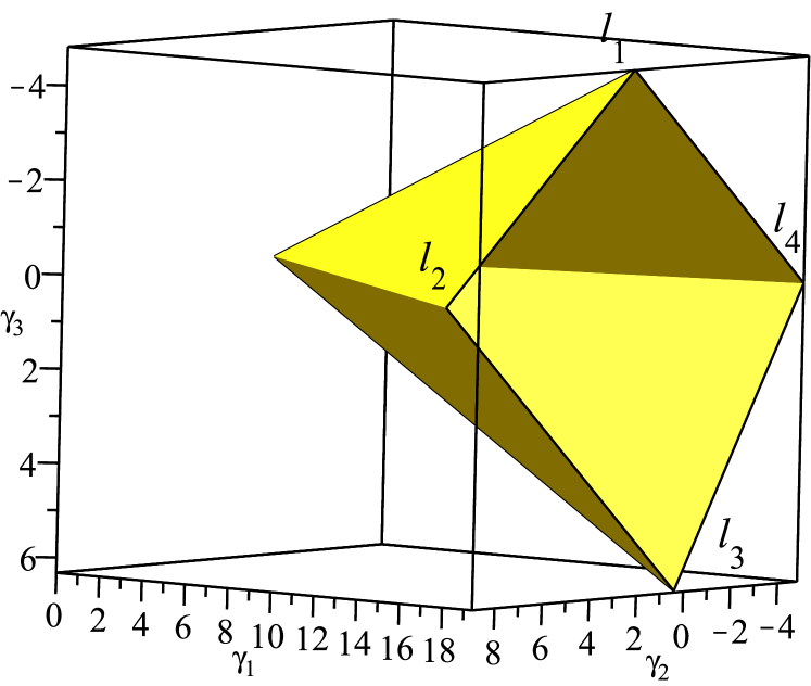
Figure 1: The part of the boundary of the feasibility region $\Lambda_{-}$ along with the edges $l_{1},l_{2},l_{3},l_{4}$ (color online).

To determine ellipticity of $H^{LK}$, we gathered in Table III the material parameters $\gamma_{1},\gamma_{2},\gamma_{3}$ for GaAs, AlAs, InAs, GaP, AlP, InP, GaSb, AlSb, InSb, GaN, AlN, InN, C and evaluated $\lambda_{1}$, $\lambda_{2}$, $\lambda_{3}$, $\lambda_{4}$ for the gathered triplets. As it turned out, the eigenvalues $\lambda_{1}$, $\lambda_{2}$, $\lambda_{4}$ are negative for all analysed parameter sets. In that case the ellipticity is determined by the value $\lambda_{3}$. We provide the values of $\lambda_{3}/E$ along with two other parameter dependent quantities which are important for the current work’s ellipticity analysis. The first is the distance $d$ from the parameter triplet $(\gamma_{1},\gamma_{2},\gamma_{3})$ to $\Lambda_{-}$. Second is an absolute ratio $\rho$ between positive and negative values of $\lambda_{1}$, $\lambda_{2}$, $\lambda_{3}$, $\lambda_{4}$.

Table 1: The material parameters for ZB type crystals, $d$ – distance from the point $(\gamma_{1},\gamma_{2},\gamma_{3})$ to the feasibility region $\Lambda_{-}$

file=ZB_6x6_gamma_lambda_d_rhoSS.csv, no head, column names reset, column count=25, column names=2=, 3=, 4=, 5=, 6=, 7=, 8=, 9=,10=, 11=, 12=, 13=, 13=, 14=, 15=, 16=, 17=, 18 = , 19 =, 20=, 21=, 22=, 23=, 24=, before reading=, tabular=r—l—SSS—SS[table-figures-integer = 1, table-figures-decimal = 3, round-precision = 3]S[table-figures-integer = 1, table-figures-decimal = 3, round-precision = 3]—r—l—SSS—SS[table-figures-integer = 1, table-figures-decimal = 3, round-precision = 3]S[table-figures-integer = 1, table-figures-decimal = 3, round-precision = 3], table head=# El $\gamma_{1}$ $\gamma_{2}$ $\gamma_{3}$ $\lambda_{3}/E$ $d$ $\rho$ # El $\gamma_{1}$ $\gamma_{2}$ $\gamma_{3}$ $\lambda_{3}/E$ $d$ $\rho$
, command= 0+22 , filter = $\thecsvinputline>1$ $\thecsvinputline<25$, table foot=,

• Set 1 from LB1

• Set 2 from LB1

• Set 3 from LB1

• Set 4 from LB1

• Set 5 from LB1

• Set 6 from LB1

• Obtained by extrapolation from 5-level model

• Measured at $T=300K$

• Set from Madelung2004

• The sets from Vurgaftman2001 LB1

From Table III one can observe that among all analysed materials only carbon has admissible sets of parameters ( the last two sets from of Table III indicated by 0 in the $\rho$ column ). All other gathered parameters yield $\lambda_{3}>0$. That is why the Hamiltonian $H^{LK}$ is not elliptic for the corresponding materials. It may even have no symmetric domain $D(H^{LK})$ as opposed to the original partial differential operator $H_{0}$. Moreover, instead of the inclusion $D(H^{LK})=D(H)\subset D(H_{0})\subset\mathcal{H}^{3}(\Omega)$ we have only

$$D(H^{LK})=D(H)\subset\mathcal{H}^{1}(\Omega).$$ (8)

It means that the discontinuous solutions of (1) are theoretically possible. They will occur in the models with jump discontinuous coefficientsCourant1956, which is the case for heterostructure materials. Additionally, the double degeneracy of $\lambda_{3}>0$ from (7) means that for certain $\Omega$ there exists a two-dimensional manifold of $D(H^{LK})$ with non-physical in terms of (8) solutions to (1). Thus, the momentum operator from (1), will be ill-defined for such eigenstates of $H^{LK}$ (by the embedding theorems, [p. 119, Egorov11998]). All the above arguments allow us to conclude that the $H^{LK}$ does not provide a sufficiently good approximation to $H_{0}$, preserving the type of the PDO, for the most of available data.

Let us return to the feasible parameters from Table III. For carbon the parameter values were analyzed earlierReggiani1983 and it was noted that they don’t agree well with the Hall effect experimental measurements. In the earlier workkpEllptArxSytnyk2010 we showed that experimentally consistent sets for C are not admissible in terms of ellipticity.

Concerning the rest of the materials from Table III we observe a clear correlation between the average distance to $\Lambda_{-}$ per material and the size of the fundamental bandgap. Namely the sets for the large-bandgap materials: AlP, AlAs, GaP, GaN, InP are noticeably close ($d<1$) to $\Lambda_{-}$. The closest in terms of the distance set number 19 for AlP can be made elliptic by the direct adjustment. Other materials have smaller gap and as a consequence are further away. The average distance to $\Lambda_{-}$ for GaAs is around 1.7. For InAs the distance is more than 6. The indium antimonide is an extreme case here, having distance of more than 12. This material has the smallest bandgap and the high curvature of light-hole bands. It is known from the experimentsKane1957; Pidgeon1966; Cardona1986 that the valence-band-only Luttinger-Kohn model is insufficient for InSb like materials, and presented analysis support this fact theoretically. The ellipticity of the higher band $k\cdot p$ models are considered in the next sections.

IV Eight-band Hamiltonians

This section is devoted to the analysis of Kane modelKane1982; kp8ProperKane_Bahder90. The basis set of $8\times 8$ Kane Hamiltoniankp8ProperKane_Bahder90 contains two more elements $\left|S\uparrow\right\rangle$ and $\left|S\downarrow\right\rangle$ in addition to the basis set of $H^{LK}$. These new elements of basis represent the influence of the innermost conduction band. Recall that the influence of the out-of-basis states is again treated perturbatively up to the second order by using the Löwding perturbation theory. In this section we will follow the exposition of [kp8ProperKane_Bahder90], because it presents the most general description of $8\times 8$ Kane Hamiltonian for zinc blende crystals. Naturally, the results presented here remain valid for other versionsVoonWillatzen2009; Birner2014; Bastos2016 of the same Hamiltonian. Since our main focus is to check the ellipticity conditions we shall drop the spin-orbit interaction part, labelled as $H_{s.o.}+H^{\prime}_{s.o.}$ in eq. (13) from [kp8ProperKane_Bahder90]. This part of the Hamiltonian is linear in $k$ and therefore won’t affect the form of $G$. (as we have mentioned before, only second order terms in $k$ are essential for ellipticity analysis) Then, following KaneKane1982, we rewrite the resulting operator in the block-diagonal form

$$H^{K}=\left(\begin{array}[]{cc}H^{K}_{\uparrow}&0\\ 0&H^{K}_{\downarrow}\\ \end{array}\right),$$

where $H^{K}_{\uparrow}$ is the Kane $4\times 4$ interaction matrix Kane1957, given by (9) in the basis $\left|S\uparrow\right\rangle,\left|X\uparrow\right\rangle,\left|Y\uparrow\right\rangle,\left|Z\uparrow\right\rangle$kp8ProperKane_Bahder90. The matrix $H^{K}_{\downarrow}$ that is also defined by (9), acts upon the spin-down part of the basis $\left|S\downarrow\right\rangle,\left|X\downarrow\right\rangle,\left|Y\downarrow\right\rangle,\left|Z\downarrow\right\rangle$.

$$H^{K}_{\uparrow}=\left(\begin{array}[]{cccc}E_{c}+\left(E+A^{\prime}\right)\mathbf{k}^{2}&iP_{0}k_{x}+Bk_{y}k_{z}&iP_{0}k_{y}+Bk_{x}k_{z}&iP_{0}k_{z}+Bk_{x}k_{y}\\[12.0pt] -iP_{0}k_{x}+Bk_{y}k_{z}&\parbox{71.13188pt}{$E_{v}+M^{\prime}(k_{y}^{2}+k_{z}^{2})$ $+L^{\prime}k_{x}^{2}+E\mathbf{k}^{2}$}&N^{\prime}k_{x}k_{y}&N^{\prime}k_{x}k_{z}\\[12.0pt] -iP_{0}k_{y}+Bk_{x}k_{z}&N^{\prime}k_{x}k_{y}&\parbox{71.13188pt}{$E_{v}+M^{\prime}(k_{y}^{2}+k_{z}^{2})$ $+L^{\prime}k_{x}^{2}+E\mathbf{k}^{2}$}&N^{\prime}k_{y}k_{z}\\[12.0pt] -iP_{0}k_{z}+Bk_{x}k_{y}&N^{\prime}k_{x}k_{z}&N^{\prime}k_{y}k_{z}&\parbox{71.13188pt}{$E_{v}+M^{\prime}(k_{y}^{2}+k_{z}^{2})$\\ $+L^{\prime}k_{x}^{2}+E\mathbf{k}^{2}$}\\ \end{array}\right).$$ (9)

Parameters $A^{\prime},B,P_{0},M^{\prime},N^{\prime},L^{\prime}$ are known as Kane parametersKane1982, their definitions are provided in Table 4.2 of VoonWillatzen2009. The quantities $E_{c}$ and $E_{v}$ are the conduction- and valence-band energies correspondingly, $E$ is equal to $\frac{\hbar^{2}}{2m_{0}}$, as before. The parameter $A^{\prime}$ represents the influence of the higher bands on the conduction band included into the basis. The parameter $P_{0}$ accounts for a mixing of conduction and valence band states away from $\bf k=0$. $B$ is a so-called inversion asymmetry parameter. It is equal to zero in the materials with centrosymmetric crystal structure like diamond kp8ProperKane_Bahder90. By setting $B=0$ in (9) we obtain a simplified version of (9) that is known as Bir-Pikus $4\times 4$ Hamiltonian. The general case of $H_{K}$ when $B\neq 0$ was studied by T. Bahder ( Eq. (15) in [kp8ProperKane_Bahder90]). In practice the mentioned parameters are fitted to experimental data; It is frequently assumed in the literature that the simplified version of $H_{K}$ provides a sufficiently good description of the physical phenomena in ZB crystals with face-centered lattice too. As we will later demonstrate, the Hamiltonian of such simplified model is non-elliptic for all studied material parameter sets and therefore is prone to the appearance of spurious solutions. The parameter $B$ can not be set to zero for the materials where $E+A^{\prime}<0$.

Similarly to the $6\times 6$ case, it is common to rewrite Hamiltonian $H^{K}$ in the basis where its spin-orbit interaction part becomes diagonal. Usually one additionally pre-multiplies the original basis functions to make inter-band matrix elements and possibly other physically relevant quantities real-valued.

Direct calculation of eigenvalues for the quadratic form associated with $H^{K}_{\uparrow}$, described in details for the Luttinger–Kohn case from the previous section, gives us five distinct eigenvalues

$$\begin{array}[]{rl}\lambda^{\prime}_{1}&=E+L^{\prime}+N^{\prime},\\ \lambda^{\prime}_{2}&=E+L^{\prime}-\frac{1}{2}N^{\prime},\\ \lambda^{\prime}_{3}&=E+M^{\prime}-\frac{1}{2}N^{\prime},\\[2.0pt] \lambda^{\prime}_{4}&=E+\frac{2A^{\prime}+2M^{\prime}+N^{\prime}}{4}-\sqrt{\frac{(2A^{\prime}-2M^{\prime}-N^{\prime})^{2}}{16}+\frac{B^{2}}{2}},\\[2.0pt] \lambda^{\prime}_{5}&=E+\frac{2A^{\prime}+2M^{\prime}+N^{\prime}}{4}+\sqrt{\frac{(2A^{\prime}-2M^{\prime}-N^{\prime})^{2}}{16}+\frac{B^{2}}{2}}.\\[2.0pt] \end{array}$$ (10)

The presence of the second order conduction-valence band mixing, characterized by the parameter $B$ of Kane Hamiltonian (9), is reflected in (10) by the pair of eigenvalues $\lambda^{\prime}_{1}$, $\lambda^{\prime}_{5}$, which are both determined by the whole set of the principal Hamiltonian parameters $N,M,L,A^{\prime},B$. Note that, if one removes the mixing by setting $B=0$, this property disappears and the eigenvalues $\lambda^{\prime}_{4}$, $\lambda^{\prime}_{5}$ are turned into

$$\lambda^{\prime}_{04}=E+M^{\prime}+\frac{1}{2}N^{\prime},\quad\lambda^{\prime}_{05}=E+A^{\prime}.$$

IV.1 Ellipticity analysis in the absence of inversion asymmetry

We analyze the set $\lambda^{\prime}_{1},\lambda^{\prime}_{2},\lambda^{\prime}_{3},\lambda^{\prime}_{04},\lambda^{\prime}_{05}$ associated with $B=0$ in $H^{K}$ first. The fifth eigenvalue $\lambda^{\prime}_{05}$ in (10) is related to the conduction band of (9) because its corresponding three-dimensional eigenspace ($\lambda^{\prime}_{05}$ is triple degenerate) has only 3 first coordinates not equal to zero. Hence this eigenspace is orthogonal to the space associated with the valence bands. Those are characterized by the eigenvalues $\lambda^{\prime}_{1}$, $\lambda^{\prime}_{2}$, $\lambda^{\prime}_{3}$, $\lambda^{\prime}_{04}$ with degeneracy 1, 2, 3, 3, respectively. The following system of inequalities ensures ellipticity of $8\times 8$ ZB Hamiltoniankp8ProperKane_Bahder90 with zero $B$

$$\left\{\begin{array}[]{rc}E+L^{\prime}+N^{\prime}&<0\\[2.0pt] E+L^{\prime}-\frac{1}{2}N^{\prime}&<0\\[2.0pt] E+M^{\prime}-\frac{1}{2}N^{\prime}&<0\\[2.0pt] E+M^{\prime}+\frac{1}{2}N^{\prime}&<0\\[2.0pt] E+A^{\prime}&>0.\end{array}\right.$$ (11)

As we mentioned, the eigenvalues $\lambda^{\prime}_{1},\lambda^{\prime}_{2},\lambda^{\prime}_{3},\lambda^{\prime}_{04}$ are related to the valence band, hence the sign of the first four innequalities from (11) is the same as in (6). The opposite sign of the fifth inequality reflects its correspondence to the conduction band. Due to the electron-hole duality, the conduction band eigen-energies need to be semi-bounded from below. The presence summand $E$ in system (11) is connected with the differences in the definition of Dresselhaus parametersDresselhaus1955 and $L^{\prime},M^{\prime}$kp8ProperKane_Bahder90.

To compare the result for the $8\times 8$ ZB Hamiltonian with the previously obtained results for the $6\times 6$ Hamiltonian we define the dimensionless parameters $\gamma^{\prime}_{1},\gamma^{\prime}_{2},\gamma_{3}^{\prime}$ similar to the Luttinger triplet Pidgeon1966; VoonWillatzen2009; Birner2014

$$\gamma^{\prime}_{1} = -\frac{1}{3}(L^{\prime}+2M^{\prime})\frac{2m_{0}}{\hbar^{2}}-1$$

$$\gamma^{\prime}_{2} = -\frac{1}{6}(L^{\prime}-M^{\prime})\frac{2m_{0}}{\hbar^{2}}$$

$$\gamma^{\prime}_{3} = -\frac{1}{6}N^{\prime}\frac{2m_{0}}{\hbar^{2}}.$$

Hereby, the system (11) is transformed to

$$\left\{\begin{array}[]{rc}-\gamma^{\prime}_{1}-4\gamma^{\prime}_{2}-6\gamma^{\prime}_{3}&<0\\[2.0pt] -\gamma^{\prime}_{1}-4\gamma^{\prime}_{2}+3\gamma^{\prime}_{3}&<0\\[2.0pt] -\gamma^{\prime}_{1}+2\gamma^{\prime}_{2}+3\gamma^{\prime}_{3}&<0\\[2.0pt] -\gamma^{\prime}_{1}+2\gamma^{\prime}_{2}-3\gamma^{\prime}_{3}&<0\\[2.0pt] 1+A&>0,\end{array}\right.$$ (12)

with $A=A^{\prime}/E$.

The modified and the original Luttinger parameters $\gamma_{1},\gamma_{2},\gamma_{3}$ are connected by the formulas Pidgeon1966

$$\gamma^{\prime}_{1}=\gamma_{1}-\frac{E_{p}}{3E_{g}},\ \gamma^{\prime}_{2}=\gamma_{2}-\frac{E_{p}}{6E_{g}},\ \gamma^{\prime}_{3}=\gamma_{3}-\frac{E_{P}}{6E_{g}},$$ (13)

where $E_{p}=P_{0}^{2}/E$, $E_{q}=E_{c}-E_{v}$ is a fundamental bandgap energy, $P_{0}$ is the Kane parameter from (9).

As it was expected, four out of five obtained inequalities (12), which represent the ellipticity constrains for the valence band part of $H^{K}$, have the structure equivalent to that for the LK Hamiltonian (7). Hence, the feasibility region of the valence-band part of $H^{K}$ in the space of parameters $(\gamma^{\prime}_{1},\gamma^{\prime}_{2},\gamma^{\prime}_{3})$ coincides with the feasibility region $\Lambda_{-}$ of $H^{LK}$, depicted in FIG. 1. It means that if $(\gamma^{\prime}_{1},\gamma^{\prime}_{2},\gamma^{\prime}_{3})\in\Lambda_{-}$, the valence-band part of the Hamiltonian $H^{K}$ in the position representation is an elliptic partial differential operator. Then, the transformation given by (13) can be geometrically interpreted as a shift in the space of parameters proportional to vector $\mathbf{v^{\prime}}=(-2,-1,-1)$. This shift reduces the value of $\lambda^{\prime}_{3}$ and, as we shall soon see, brings the majority of the non-elliptic parameter triplets $(\gamma_{1},\gamma_{2},\gamma_{3})$ closer to the feasibility region.

The dimensionless parameter $A$ from the fifth inequality, that complements a set of ellipticity constrains (12), is responsible for a coupling between the conduction band and other states. It is commonly assumed that the in-basis valence bands are the major contributors to $A$. The value of $A$ is determined by matching its value to the effective mass of conduction band $m_{c}$, determined experimentally using the formula

$$A=\frac{m_{0}}{m_{c}}-1-E_{p}\frac{E_{g}+\frac{2}{3}\Delta}{E_{g}(E_{g}+\Delta)}.$$ (14)

The magnitude of this parameter is clearly affected by the size of band-gap $E_{g}$ and spin-splitting $\Delta$. The experimental nature of $m_{c}$ does not factor out other possible contributions to $A$. For that reason we extended the collection of parameter sets from Table III by those stemming from the same sets of Luttinger parameters and the different values of bandgap energy $E_{g}$ (measured within different experimental setups). We also added a parameter set obtained by fitting the bandstructure of $8\times 8$ Hamiltonian to the bandstructure calculated by ab-initio methodsBastos2016. All the data pertaining to the ellipticity analysis of $8\times 8$ Hamiltonian is collected in Table IV.1. In each case the modified Luttinger parameters $\gamma^{\prime}_{1},\gamma^{\prime}_{2},\gamma_{3}^{\prime}$ were calculated by using (13) and the values of $P_{0}^{2}$, $E_{g}$ provided in the dataset source. For those sources from the table that have $P_{0}^{2}$ unavailable we use the values collected by I. Vurgaftman, J. R.  Meyer and L. R Ram-MohanVurgaftman2001.

Table 2: The material data for $8\times 8$ ZB Hamiltonian with $B=0$, $d$ – distance from the point $(\gamma_{1},\gamma_{2},\gamma_{3})$ to the feasibility region $\Lambda_{-}$. The positive values of $\lambda^{\prime}_{1}/E-\lambda^{\prime}_{05}/E$ are printed in bold.

file=ZB_8x8_gamma_lambda_d_rho.csv, no head, column count=21, column names reset, column names=2=, 3=, 4=, 5=,6=, 7=, 8=, 9=,10=, 11=,12=, 13=, 14=, 15=, 16=, 17=, 18=, 19=, 20=, 21=, before reading=, tabular=r—l—SS[table-format=1.2]S[round-precision = 3, table-format=0.3]SS[table-format=2.2]SS—SSSSSS[table-format=1.2]S[table-format=1.2]—S[table-format=1.2]S[table-format=0.2], table head=# El $E_{p}$ $E_{g}$ $\Delta_{SO}$ $A^{\prime}$ $\gamma^{\prime}_{1}$ $\gamma^{\prime}_{1}$ $\gamma^{\prime}_{3}$ $\lambda^{\prime}_{1}/E$ $\lambda^{\prime}_{2}/E$ $\lambda^{\prime}_{3}/E$ $\lambda^{\prime}_{04}/E$ $\lambda^{\prime}_{05}/E$ $d$ $\rho$ $\Delta_{05}^{\text{min}}$ $\Delta_{05}^{\text{max}}$
, before line=, command=1 , table foot=, filter = $\thecsvinputline>1$ $\thecsvinputline<53$

• Set 1 from LB1

• Set 2 from LB1

• Set 3 from LB1

• Set 4 from LB1

• Set 5 from LB1

• Set 6 from LB1

• Obtained by extrapolation from 5-level model

• Measured at $T=300K$

The ellipticity conditions of $H^{K}$ are still violated for all materials presented in Table III. The situation is, however, more complex than for the $6\times 6$ Hamiltonian. To illustrate that, we supplied in Table IV.1 the values of $\lambda^{\prime}_{1}-\lambda^{\prime}_{05}$, the distance $d$ to the feasibility region from $(\gamma^{\prime}_{1},\gamma^{\prime}_{2},\gamma^{\prime}_{3})$ and the measure of non-ellipticity $\rho$ which is defined in the same way as for the $6\times 6$ Hamiltonian case.

Overall, we can confirm the reduction of average distance to the feasibility region for all materials, especially for InAs and InSb. Furthermore, for several materials there exist parameter sets that are close to satisfy the full set of ellipticity constraints described by (12). Those are narrow gap semiconductor InSb (sets #LABEL:mp:ZBK:InSb_LB1_1; #LABEL:mp:ZBK:InSb_LB1_2 from Table IV.1) and, perhaps more surprisingly, the materials with larger band-gap InP, AlAs and AlSb ( sets #LABEL:mp:ZBK:InP_LB1_2, #LABEL:mp:ZBK:AlAs_LB1;#LABEL:mp:ZBK:AlAs_Mad, and #LABEL:mp:ZBK:AlSb_Vurg1). For these materials the corresponding parameter sets can be made elliptic by direct adjustment of $\gamma^{\prime}_{1},\gamma^{\prime}_{2},\gamma^{\prime}_{3},A$.

Certain parameter sets for AlP, AlSb and InAs satisfy ellipticity conditions for the valence band part of the Hamitonian and do not satisfy the conduction-band constraint (inequality 5 from (12)). Among those, the sets #LABEL:mp:ZBK:AlP_Vurg1, #LABEL:mp:ZBK:AlSb_Vurg1 for AlP, AlSb reported in [Vurgaftman2001] differ sharply in the size of $\gamma_{2}$ from two other sets for these materials collected in Table IV.1. For AlP this can explained by the fact that in the absence of direct experimental data most of the material parameters were extrapolated from measurements for ternary alloys and ab-initio calculations which carries a lot of uncertainty. The authors of [Vurgaftman2001] performed readjustment of the Luttinger parameters to better match the experimental photoluminescence results on AlP$/$GaP heterostructuresIssiki1995. The set #LABEL:mp:ZBK:AlSb_Vurg1 for AlSb is based on the available theoretical calculations from various sources and the simultaneous fitting of $\gamma_{1},\gamma_{2},\gamma_{3}$ to the experimentally-determined hole effective masses along [001], [110] and [111] directions Vurgaftman2001.

For InAs we can judge from the size of $\lambda^{\prime}_{1}-\lambda^{\prime}_{04}$ that the triplets $(\gamma^{\prime}_{1},\gamma^{\prime}_{2},\gamma^{\prime}_{3})$ of its parameter sets are right near the side of $\Lambda_{-}$ described by $\lambda^{\prime}_{2}=0$. Two are inside (sets #LABEL:mp:ZBK:InAs_Vurg1;#LABEL:mp:ZBK:InAs_LB1_1) and two others are slightly off (sets #LABEL:mp:ZBK:InAs_LB1_2;#LABEL:mp:ZBK:InAs_Mad). The values of $\lambda^{\prime}_{05}$ for all four parameter sets are grouped near the value $\lambda^{\prime}_{05}=-4.8$ and thus the conduction part of the Hamiltonian is, again, far from being elliptic.

All material parameter sets for GaAs violate two out of four ellipticity conditions for the valence-band part, although one parameter set #LABEL:mp:ZBK:GaAs_LB1_2 from Table IV.1 stays close to $\Lambda_{-}$ ($d=$0.341\,226\,582\,094\,873$$). However, it violates the ellipticity condition for the conduction-band part by the same margin of approximately $-2.9$ as do other sets of GaAs parameters, let alone set #LABEL:mp:ZBK:GaAs_Bastos where the margin is slightly lower: $\lambda^{\prime}_{05}\approx-2.34$. The indicated reduction of margin should be attributed to the optimization procedureBastos2016 used to acquire set #LABEL:mp:ZBK:GaAs_Bastos. As far as the ellipticity is concerned, this optimization procedure is no more effective than other acquisition methods.

The sets for GaN and AlN are failing first two valence-part constraints from (12) just like the most of the other material parameters. One exception is the set number LABEL:mp:ZBK:GaN_Cardona for GaNCardona_05, where the spherical symmetry of the heavy-hole and the light-hole bands is assumed. This assumption leads to the larger values of $\gamma_{1},\gamma_{3}$ and smaller $\gamma_{2}$; and, as a consequence, more than five times smaller ratio $\rho$ between positive and negative eigenvalues.

Even a more severe situation is observed for InN. The conduction-band eigenvalue $\lambda^{\prime}_{05}$ is noticeably below zero for all three available datasets ($\lambda^{\prime}_{05}\approx$-4.540\,020\,413\,713\,21$$; $-7.718\,749\,756\,966\,31$; $-2.873\,123\,167\,251\,18$ for sets #LABEL:mp:ZBK:InN_Vurg1; #LABEL:mp:ZBK:InN_Vurg2; #LABEL:mp:ZBK:InN_Rinke accordingly). In addition, three out of four valence-band conditions are violated. It is important to highlight that the recently obtained set of parameters #LABEL:mp:ZBK:InN_Rinke features roughly two times larger values of $\gamma_{1},\gamma_{2}$ and $\gamma_{3}$ and noticeably smaller $E_{p},E_{g}$ than two other sets #LABEL:mp:ZBK:InN_Vurg1, #LABEL:mp:ZBK:InN_Vurg2 reported earlierVurgaftman2001; Vurgaftman2003. As demonstrated in [Rinke2008] set #LABEL:mp:ZBK:InN_Rinke recovers bandstructure better than two others sets for InN, discussed above. In terms of ellipticity, this set results in a lower, than others, distance to $\Lambda_{-}$ ($d\approx$0.842\,567\,107\,552\,504$$) and lower $\lambda^{\prime}_{05}\approx$0.169\,245\,283\,018\,868$$.

For GaP and GaSb the data seem inconclusive as the size and the sign of eigenvalues (10) are dependant on the choice the material parameter dataset. Sets #LABEL:mp:ZBK:GaP_LB1_1, #LABEL:mp:ZBK:GaSb_LB1_1 from Landolt-BörnsteinLB1, based on the earlier data of P. Lawaetzkp7Lawaetz71, are most favourable in terms of ellipticity: $d\approx$0.140\,059\,606\,511\,186$$, $\lambda^{\prime}_{05}\approx$0.053\,418\,803\,418\,803$$ for GaP; $d\approx$0.324\,200\,259\,259\,466$$, $\lambda^{\prime}_{05}\approx$2.392\,272\,659\,026\,08$$ for GaSb. As a summary of the above analysis, we visualize in FIG. 2 the values of $\lambda^{\prime}_{05},d$ for the selected parameter sets with the material-wise minimal distance to $\Lambda_{-}$. In this figure the ellipticity of Hamiltonian is depicted by the region (shaded in gray) where $\lambda^{\prime}_{05}>0$ and $d<0$ simultaneously.

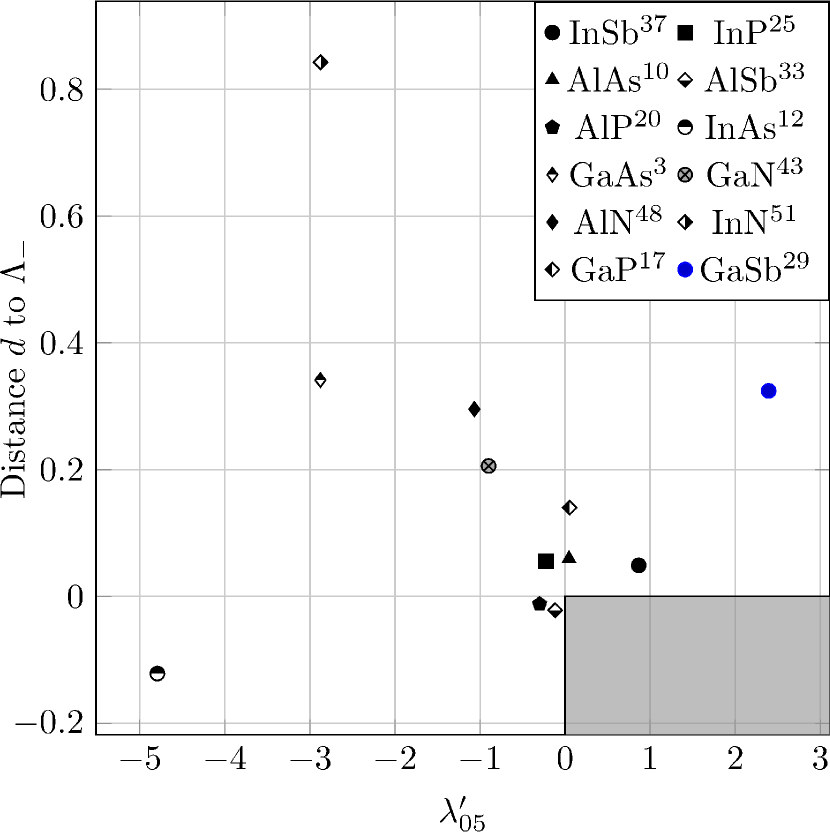
Figure 2: The values of quantities $\lambda^{\prime}_{05},d$ for the list of selected material parameter sets from Table IV.1 (color online). The shaded region indicates pairs $(\lambda^{\prime}_{05},d)$ based on the elliptic parameters of $8\times 8$ modelkp8ProperKane_Bahder90

It is worth noticing that roughly $76$\mathrm{\char 37\relax}$$ of parameter sets for analyzed materials fail the conduction-band constraint $\lambda^{\prime}_{05}>0$. This group includes all datasets for GaAs, InAs, AlP, AlSb, GaN, AlN, InN, quite important for applications. The positive (negative) sign of $\lambda^{\prime}_{05}$ is responsible for positive(negative) gain in the energy as we go from one conduction-band eigenvalue of Hamiltonian to the next in the position representation. In the momentum representation, the eigenvalue’s sign and its magnitude is responsible for upward (downward) curvature of conduction band. In addition to the highlighted in section III issues caused by the non-ellipticity of valence-band part of the Hamiltonian $H^{K}$, the violation of condition $\lambda^{\prime}_{05}>0$ entails the existence of conduction-band related eigenstates of $H^{K}$ with energies in the band-gap or the regions related to valence bandsVeprek07; Veprek08; foreman_sp_07; Birner2014. This obviously poses a serious problem in applications.

A rescaling procedure was introduced by B. Foreman in [Foreman_sp_97] (see also the work of S. Birner [Birner2014]) and has been adoptedVinas2017; Birner2007 ever since as a way to make $\lambda^{\prime}_{05}$ positive and avoid the above-described type of spurious solutions. The idea of the procedure is to adjust the momentum matrix element $E_{p}$ so that $\lambda^{\prime}_{05}$ is no longer negative. Let us assume that we target some value of $\lambda^{\prime}_{05}=a$. Then, by using the definition of $\lambda^{\prime}_{05}$ and (14), we obtainBirner2014

$$E_{p}=\left(\frac{m_{0}}{m_{c}}-a\right)\frac{E_{g}(E_{g}+\Delta_{SO})}{E_{g}+\frac{2}{3}\Delta_{SO}}.$$ (15)

Two values $a=0$ and $a=1$ are considered in the literature as a target for rescaling. The new value of $E_{p}$ will necessary affect the values of modified Luttinger parameters $\gamma^{\prime}_{1},\gamma^{\prime}_{2},\gamma^{\prime}_{3}$ which are defined by (13). To figure out how this procedure would impact the ellipticity of the entire $8\times 8$ ZB Hamiltonian $H^{K}$ one needs to rewrite eigenvalues $\lambda^{\prime}_{1}-\lambda^{\prime}_{04}$ as functions of $E_{p},E_{g}$:

$$\lambda^{\prime}_{1}=\lambda_{1}+2E\frac{E_{p}}{E_{g}},\ \lambda^{\prime}_{2/04}=\lambda_{2/4}+\frac{E}{2}\frac{E_{p}}{E_{g}},\ \lambda^{\prime}_{3}=\lambda_{3}-\frac{E}{2}\frac{E_{p}}{E_{g}}.$$

By combining the above representations with (15) we obtain a new version of ellipticity constraints (12) for the valence-band part of $H^{K}$

$$\lambda_{1}+2E_{m}-\frac{2a}{E_{r}}<0,\quad\lambda_{2}+\frac{1}{2}E_{m}-\frac{a}{2E_{r}}<0,$$ (16)

$$\lambda_{3}-\frac{1}{2}E_{m}+\frac{a}{2E_{r}}<0,\quad\lambda_{4}+\frac{1}{2}E_{m}-\frac{a}{2E_{r}}<0,$$

where $E_{m}=\dfrac{m_{0}}{m_{c}E_{r}}$, $E_{r}=\dfrac{E_{g}+\frac{2}{3}\Delta_{SO}}{E(E_{g}+\Delta_{SO})}$ are two material-dependent constants. Now we substitute back $a=\lambda^{\prime}_{05}+\Delta_{05}$ and solve system of inequalities (16) with respect to $\Delta_{05}$. As a result, it will give us the range for the values of the rescaling parameter $\Delta_{05}$ that make the valence-band part of Kane Hamiltonian elliptic

$$E_{r}\max\left\{\frac{1}{2}\lambda^{\prime}_{1},2\lambda^{\prime}_{2},2\lambda^{\prime}_{04}\right\}<\Delta_{05}<-2\lambda^{\prime}_{3}E_{r}.$$ (17)

The calculated values for the ranges from (17) are provided in the last two columns of Table IV.1. If $-\lambda^{\prime}_{05}<-2\lambda^{\prime}_{3}E_{r}$, then the Hamiltonian can be made elliptic by setting $\Delta_{05}$ to the arbitrary value within range (17) so that $\lambda^{\prime}_{05}+\Delta_{05}$ is positive. In practice one would also like to make sure that the numerical inaccuracies introduced by the eigenvalue calculation procedure for $H^{K}$ will not overturn any of the signs of $\lambda^{\prime}_{1}$ – $\lambda^{\prime}_{05}$. To minimize that possibility and to keep $\Delta_{05}$ reasonably small we suggest the following formula for the selection of $\Delta_{05}$

$$\Delta_{05}=\begin{cases}2\Delta_{m}+0.1,\quad&\Delta_{m}+\lambda^{\prime}_{3}E_{r}<-0.1,\\ \Delta_{m}-\lambda^{\prime}_{3}E_{r},\quad&\text{otherwise}.\end{cases}$$ (18)

with $\Delta_{m}=\max\left\{\frac{1}{4}\lambda^{\prime}_{1}E_{r},\lambda^{\prime}_{2}E_{r},\lambda^{\prime}_{04}E_{r},-\dfrac{\lambda^{\prime}_{05}}{2E}\right\}$.

We carried out the rescaling procedure for the material parameters from Table IV.1 and selected the sets with minimal $\Delta_{05}$ for every given material. The resulting values of readjusted $E_{p}$, $A^{\prime}$ along with new values of modified Luttinger parameters are presented in Table IV.1. It is also worth noting that the resulting value of $1+A$ in our case is never equal to zero or one, as it was usually assumed by authors beforeForeman_sp_97; Birner2014. For many materials the value of adjusted parameter $A$ is greater than 0.

To see the impact of rescaling on the band dispersion, in Table IV.1 we also supplied a maximum absolute difference (adjustment error) between the corresponding bands of bandstructure calculated over the 20% of three high symmetry paths $\Gamma L$, ${\Gamma K}$ and ${\Gamma X}$ pertaining to the first Brillouin zone (FBZ). Such a size of the domain for comparison is commonVurgaftman2001 and motivated by the existing evidenceBastos2016 that the accurate fit of the $k\cdot p$ bandstructure to the state-of-the-art ab-initio calculations is possible over this part of FBZ. To ascertain the band that contributes most to the error we supplied in FIG. 3 a), and FIG. LABEL:fig:ZBK_resc_bs_comp the graphical comparison of band-structure diagrams for every set from Table IV.1 and the original sets of material parameters from Table IV.1, on which they are based. For clarity, only bands with even numbers in the representation of $8\times 8$ Hamiltoniankp8ProperKane_Bahder90 are plotted in these figures.

Table 3: Selected material parameters, rescaled via (18) together with the difference between corresponding bands of $8\times 8$ Hamiltoniankp8ProperKane_Bahder90 for original and rescaled parameters

file=ZB_8x8_B_0_selected_rescaled_sort_bs_error.csv, no head, column count=17, column names reset, column names=1=, 2=, 3=, 4=,5=, 6=, 7=, 8=,9=, 10=,11=,12=, 13=, tabular=@ lS[round-precision = 2, table-format=1.2]S[round-precision = 2, table-format=1.2]S[table-format=1.2]SS[table-format=1.2]S[table-format=1.2]S[round-precision = 2, table-format=2.1]S[round-precision = 2, table-format=3.2]@ , table head=El^a $\Delta_{05}$^b

$E_{p}$ $A^{\prime}$ $\gamma^{\prime}_{1}$ $\gamma^{\prime}_{2}$ $\gamma^{\prime}_{3}$ $\lambda_{v}$^c $err$^d
, command= ^{LABEL:\thirteen} , table foot=, filter = $\thecsvinputline>1$ $\thecsvinputline<53$

• Refer to the original dataset number from Table IV.1

• The quantity $\Delta_{05}$ describes the size of adjustment to $A^{\prime}$

• The values of $\lambda_{v}$ are calculated via $\lambda_{v}=\max\{\lambda^{\prime}_{1},\lambda^{\prime}_{2},\lambda^{\prime}_{3},\lambda^{\prime}_{04}\}$

• Maximum difference in meV between the bandstrucure for the original parameters from Table IV.1 and the rescaled parameters calculated by using (18) over the 20 % of the paths $\Gamma L$, ${\Gamma K}$ and ${\Gamma X}$

\begin{overpic}[width=86.72267pt]{pic_diff_sel_resc_GaN} \put(1.0,50.0){\rotatebox{90.0}{\small Energy (eV)}} \put(12.0,2.0){\small Fraction of the path} \put(20.5,12.0){$K\leftarrow\Gamma\rightarrow L$} \put(29.0,93.0){\large GaN} \put(3.0,93.0){\large a)} \put(15.5,55.0){\hbox{\pagecolor{White}\framebox{\parbox{60.00009pt}{\tiny\begin{tabular}[]{ll}Rescaled&Original\\ {\color[rgb]{0,0,0}\rule[2.0pt]{12.0pt}{0.8pt}} \hfill CB&{\color[rgb]{0,0,0}\rule[2.0pt]{3.5pt}{0.8pt}\rule[2.0pt]{2.0pt}{0.0pt}\rule[1.95pt]{1.0pt}{1.0pt}\rule[2.0pt]{2.0pt}{0.0pt}\rule[2.0pt]{3.5pt}{0.8pt}} \hfill CB\\ {\color[rgb]{0,0,0}\rule[2.0pt]{12.0pt}{0.8pt}} \hfill HH&{\color[rgb]{0,0,0}\rule[2.0pt]{3.5pt}{0.8pt}\rule[2.0pt]{2.0pt}{0.0pt}\rule[1.95pt]{1.0pt}{1.0pt}\rule[2.0pt]{2.0pt}{0.0pt}\rule[2.0pt]{3.5pt}{0.8pt}} \hfill HH\\ {\color[rgb]{0,0,0}\rule[2.0pt]{12.0pt}{0.8pt}} \hfill LH&{\color[rgb]{0,0,0}\rule[2.0pt]{3.5pt}{0.8pt}\rule[2.0pt]{2.0pt}{0.0pt}\rule[1.95pt]{1.0pt}{1.0pt}\rule[2.0pt]{2.0pt}{0.0pt}\rule[2.0pt]{3.5pt}{0.8pt}} \hfill LH\\ {\color[rgb]{0,0,0}\rule[2.0pt]{12.0pt}{0.8pt}} \hfill SO&{\color[rgb]{0,0,0}\rule[2.0pt]{3.5pt}{0.8pt}\rule[2.0pt]{2.0pt}{0.0pt}\rule[1.95pt]{1.0pt}{1.0pt}\rule[2.0pt]{2.0pt}{0.0pt}\rule[2.0pt]{3.5pt}{0.8pt}} \hfill SO\end{tabular} }}} } \par\end{overpic}

\begin{overpic}[width=108.405pt]{pic_err_bs_resc_mEv_GaN} \put(1.0,30.0){\rotatebox{90.0}{\small Energy (meV)}} \put(25.0,2.0){\small Percent of the path} \put(45.0,90.0){\large GaN} \put(14.0,12.0){$\Gamma$} \put(-3.0,91.0){\large b)} \put(15.6,-8.0){\small CB: {\color[rgb]{1,0,0}\dottedline{1.2}(0,3)(6,3)} \hskip 3.59995pt $\Gamma L$, {\color[rgb]{1,0,0}\drawline(0,3)(3,3)\drawline(5,3)(8,3)} \hskip 4.5pt ${\Gamma K}$, {\color[rgb]{1,0,0}\drawline(0,3)(2.8,3)\drawline(3.8,3)(4.2,3)\drawline(5.2,3)(8,3)} \hskip 4.5pt ${\Gamma X}$} \put(15.3,-15.0){\small HH: {\color[rgb]{0,0,0}\dottedline{1.2}(0,3)(6,3)} \hskip 3.59995pt $\Gamma L$, {\color[rgb]{0,0,0}\drawline(0,3)(3,3)\drawline(5,3)(8,3)} \hskip 4.5pt ${\Gamma K}$, {\color[rgb]{0,0,0}\drawline(0,3)(2.8,3)\drawline(3.8,3)(4.2,3)\drawline(5.2,3)(8,3)} \hskip 4.5pt ${\Gamma X}$} \put(16.0,-22.0){\small LH: {\color[rgb]{0,0,1}\dottedline{1.2}(0,3)(6,3)} \hskip 3.59995pt $\Gamma L$, {\color[rgb]{0,0,1}\drawline(0,3)(3,3)\drawline(5,3)(8,3)} \hskip 4.5pt ${\Gamma K}$, {\color[rgb]{0,0,1}\drawline(0,3)(2.8,3)\drawline(3.8,3)(4.2,3)\drawline(5.2,3)(8,3)} \hskip 4.5pt ${\Gamma X}$} \put(16.0,-29.0){\small LH: {\color[rgb]{0,0,0}\dottedline{1.2}(0,3)(6,3)} \hskip 3.59995pt $\Gamma L$, {\color[rgb]{0,0,0}\drawline(0,3)(3,3)\drawline(5,3)(8,3)} \hskip 4.5pt ${\Gamma K}$, {\color[rgb]{0,0,0}\drawline(0,3)(2.8,3)\drawline(3.8,3)(4.2,3)\drawline(5.2,3)(8,3)} \hskip 4.5pt ${\Gamma X}$} \end{overpic}

Figure 3: Comparison of original and rescaled parameter sets for GaN (color online): Conduction band (CB), heavy-hole (HL), light-hole (LH) and the split-off band (SO). a) Bandstructure along the fraction of symmetry path $K-\Gamma-L$: original set LABEL:mp:ZBK:GaN_LB1 (solid), rescaled set from Table IV.1 (dashed); b) bandstructure adjustment error along the paths $\Gamma L$, ${\Gamma K}$ and ${\Gamma X}$

[column count=7, head, column names reset, column names=1=, 2=, 3=, 4=,5=, 6=, 7=, 8=, filter expr = test