On a New Improvement-Based Acquisition Function for Bayesian Optimization

Abstract

Bayesian optimization (BO) is a popular algorithm for solving challenging optimization tasks. It is designed for problems where the objective function is expensive to evaluate, perhaps not available in exact form, without gradient information and possibly returning noisy values. Different versions of the algorithm vary in the choice of the acquisition function, which recommends the point to query the objective at next. Initially, researchers focused on improvement-based acquisitions, while recently the attention has shifted to more computationally expensive information-theoretical measures. In this paper we present two major contributions to the literature. First, we propose a new improvement-based acquisition function that recommends query points where the improvement is expected to be high with high confidence. The proposed algorithm is evaluated on a large set of benchmark functions from the global optimization literature, where it turns out to perform at least as well as current state-of-the-art acquisition functions, and often better. This suggests that it is a powerful default choice for BO. The novel policy is then compared to widely used global optimization solvers in order to confirm that BO methods reduce the computational costs of the optimization by keeping the number of function evaluations small. The second main contribution represents an application to precision medicine, where the interest lies in the estimation of parameters of a partial differential equations model of the human pulmonary blood circulation system. Once inferred, these parameters can help clinicians in diagnosing a patient with pulmonary hypertension without going through the standard invasive procedure of right heart catheterization, which can lead to side effects and complications (e.g. severe pain, internal bleeding, thrombosis).

Keywords Bayesian Optimization, Global Optimization, Gaussian Processes, Pulmonary Circulation

1 Introduction

Many real-life applications such as parameter estimation and decision making in science, engineering and economics require solving an optimization problem. Traditionally the aim has been to minimize a function which is fast to query at any given point and where the gradient information is readily available or easy to estimate. More recently, new research directions involve complex and multiscale computational models that do not meet these requirements. They typically are computationally expensive, perhaps without an exact functional form, the gradient information might not be available and outputs could be corrupted by noise. Examples of these applications include parameter estimation in robotics (Calandra et al., 2016; Lizotte et al., 2007), automatic tuning of machine learning algorithms (Hutter et al., 2011; Snoek et al., 2012; Wang et al., 2013; Kotthoff et al., 2017), environmental monitoring and sensor placement (Garnett et al., 2010), soft-tissue mechanical models of the pulmonary circulation (Noè et al., 2017) and more (Shahriari et al., 2016).

Bayesian optimization (BO) is a class of algorithms designed to solve these complex optimization tasks. It is not a recent field as it dates back to the 1970–1980s, when the Lithuanian mathematician Jonas Mockus published a series of papers and a book on the topic (Mockus, 1975, 1977, 1989), but it increased in popularity only recently due to the advances in computational resources.

With the increase in computational power, modellers started developing more complex simulators of real life phenomena. For example, by switching from linear to nonlinear differential equations, adding more layers of them, and interfacing many micro-level models in order to recreate in silico macro-level phenomena. Simulators typically involve many tunable parameters. Setting these parameters by hand would be cumbersome, hence the need for an automated and principled framework to deal with them. In these models standard likelihood based inference is not straightforward due to the time required for a single forward simulation. This could involve, for example, the numerical solution of a system of nonlinear partial differential equations, hence calling for an iterative procedure. Furthermore, the maximum likelihood equations may not have an analytical solution and need to be solved iteratively, adding another level of computational complexity to the problem. Usually the likelihood landscape is highly multimodal, calling for multiple restarts, and effectively making the problem NP-hard.

Section 2 states the generic problem and reviews the main aspects of Gaussian processes and Bayesian optimization. It then summarizes the popular classes of acquisition functions found in the literature, emphasizing the line of thought that led to their development. In Section 3 we derive the variance of the improvement quantifier and use it to define a new acquisition function. It improves the literature ones by accounting for another layer of uncertainty in the problem, namely the uncertainty in the improvement random variable. Sections 4 and 5 compare the newly introduced acquisition function with state-of-the-art acquisition functions from the Bayesian optimization literature on a large set of test functions for global optimization. In Section 6 we confirm that Bayesian optimization reduces the number of function evaluations required to reach the global optimum to a certain tolerance level, compared to standard global optimization algorithms. The proposed algorithm is then used in Section 7 to infer the parameters of a partial differential equations (PDEs) model of the human pulmonary blood circulation system, with the ultimate goal to pave the way towards autonomous in silico diagnosis and prognosis. Section 8 summarizes our results.

2 Background

Suppose that the task is to minimize globally a real-valued function $f(\boldsymbol{x})$, called objective function, over a compact domain $\mathbb{X}\subset\mathbb{R}^{d}$ and that observing $f(\boldsymbol{x})$ is costly due to the need to run long computer simulations or physical experiments. The global minimum is denoted $f_{\mathrm{global}}=\min_{\boldsymbol{x}\in\mathbb{X}}f(\boldsymbol{x})$, which is attained at $\boldsymbol{x}_{\mathrm{global}}$. Here we will focus on the minimization problem as the conversion of a maximization problem into a minimization one is trivial. Many global optimization algorithms have been proposed in literature, e.g. genetic algorithms, multistart and simulated annealing methods (Locatelli and Schoen, 2013), but these algorithms require many function evaluations and hence are designed for functions that are cheap to query. Bayesian optimization (BO), instead, is an algorithm designed to optimize expensive-to-evaluate functions by keeping the number of function evaluations as low as possible, hence saving computational time. To do so, BO uses all of the information collected so far (function values and corresponding locations) to internally maintain a model of the objective function. This is used to learn about the location of the minimum, and the model is continuously updated as new information arrives. The objective function $f$ is approximated by a surrogate model or emulator, which is usually given a Gaussian process (GP) prior, see Rasmussen and Williams (2006). The values of the objective function are generally modelled according to the additive decomposition $y_{i}=f(\boldsymbol{x}_{i})+\varepsilon_{i}$, where $\varepsilon_{i}$ are i.i.d. $\mathsf{N}(0,\sigma^{2})$ errors and $f\sim\mathsf{GP}(m,k)$ is the GP prior on the regression function.

2.1 Gaussian Processes

A random process $\left\{f(\boldsymbol{x}),\,\boldsymbol{x}\in\mathbb{X}\right\}$ is said to be Gaussian if and only if every finite dimensional distribution is a Gaussian random vector. Similarly to a multivariate Normal, parametrized by a mean vector and a covariance matrix, a Gaussian process is completely specified by a mean and a covariance function, denoted by $m(\boldsymbol{x})$ and $k(\boldsymbol{x},\boldsymbol{x}^{\prime})$ respectively. They return the mean $\mathbb{E}[f(\boldsymbol{x})]=m(\boldsymbol{x})$ and the covariance $\mathrm{cov}[f(\boldsymbol{x}),f(\boldsymbol{x}^{\prime})]=k(\boldsymbol{x},\boldsymbol{x}^{\prime})$ as function of the index only. A GP prior on the random function $f$ is denoted $f(\boldsymbol{x})\sim\mathsf{GP}(m(\boldsymbol{x}),k(\boldsymbol{x},\boldsymbol{x}^{\prime}))$. In our studies we used a constant mean function: $m(\boldsymbol{x})=c$, where $c$ represents a constant to be estimated. The covariance functions considered are the ARD Matérn 5/2 kernel:

$$k_{5/2}(\boldsymbol{x},\boldsymbol{x}^{\prime})=\sigma_{f}^{2}\left(1+\sqrt{5}r+\frac{5}{3}r^{2}\right)\exp\left(-\sqrt{5}r\right),\qquad r=\sqrt{\sum_{i=1}^{d}\frac{(x_{i}-x_{i}^{\prime})^{2}}{\ell_{i}^{2}}},$$

and the ARD Squared Exponential kernel:

$$k_{\mathrm{SE}}(\boldsymbol{x},\boldsymbol{x}^{\prime})=\sigma_{f}^{2}\exp\left\{-\frac{1}{2}\sum_{i=1}^{d}\frac{(x_{i}-x_{i}^{\prime})^{2}}{\ell_{i}^{2}}\right\},$$

see Rasmussen and Williams (2006) for more details, and the two kernels gave very similar experimental results (compare Sections 5 and A.4). The acronym ARD stands for automatic relevance determination, and it refers to kernels that allow for a different lengthscale parameter $\ell_{i}$ $(i=1,\dots,d)$ in each dimension. When an input dimensionality has a large lengthscale, the function is effectively flat along that direction, meaning that the input is not relevant. The model hyperparameters, $\boldsymbol{\theta}=(c,\ell_{1},\dots,\ell_{d},\sigma_{f},\sigma)^{\top}$, are estimated by maximum marginal likelihood. In the main part of the paper we present results for the widely used ARD Squared Exponential kernel, in order to allow for a fair comparison with the competing methods, whose code is provided only for this family of covariance functions. A GP with the ARD Squared Exponential kernel models infinitely differentiable functions, while the ARD Matérn 5/2 kernel gives rise to sample paths which are only twice differentiable. Results for the ARD Matérn 5/2 kernel, recommended by Snoek et al. (2012), are shown in Appendix A.4. After having collected $n$ data points, $\mathcal{D}_{n}=\{(\boldsymbol{x}_{1},y_{1}),\dots,(\boldsymbol{x}_{n},y_{n})\}$, the predictive distribution of $f$ is again a GP with mean $\hat{f}(\boldsymbol{x})$ and covariance $s(\boldsymbol{x},\boldsymbol{x}^{\prime})$:

$$f(\boldsymbol{x})\mid\mathcal{D}_{n} \sim\mathsf{GP}(\hat{f}(\boldsymbol{x}),s(\boldsymbol{x},\boldsymbol{x}^{\prime}))$$ (1)

$$\hat{f}(\boldsymbol{x}) =m(\boldsymbol{x})+\boldsymbol{k}(\boldsymbol{x})^{\top}[\boldsymbol{K}+\sigma^{2}\boldsymbol{I}]^{-1}(\boldsymbol{y}-\boldsymbol{m})$$

$$s(\boldsymbol{x},\boldsymbol{x}^{\prime}) =k(\boldsymbol{x},\boldsymbol{x}^{\prime})-\boldsymbol{k}(\boldsymbol{x})^{\top}[\boldsymbol{K}+\sigma^{2}\boldsymbol{I}]^{-1}\boldsymbol{k}(\boldsymbol{x}^{\prime}),$$

where $\boldsymbol{K}=[k(\boldsymbol{x}_{i},\boldsymbol{x}_{j})]_{i,j=1}^{n}$ is the $n$-by-$n$ covariance matrix at the training inputs, $\boldsymbol{k}(\boldsymbol{x})=[k(\boldsymbol{x}_{1},\boldsymbol{x}),\dots,k(\boldsymbol{x}_{n},\boldsymbol{x})]^{\top}$ is the column vector of size $n$-by-$1$ containing the covariances between each of the training inputs and the test point $\boldsymbol{x}$, while $\boldsymbol{m}=[m(\boldsymbol{x}_{1}),\dots,m(\boldsymbol{x}_{n})]^{\top}$ represents the mean at the training inputs. The posterior variance is readily obtained as $s^{2}(\boldsymbol{x})=s(\boldsymbol{x},\boldsymbol{x})=\mathrm{cov}[f(\boldsymbol{x}),f(\boldsymbol{x})]$.

2.2 Bayesian Optimization

The strength of BO lies in the following problem shift. Instead of directly optimizing the expensive objective function $f$, the optimization is performed on an inexpensive auxiliary function which uses the available information in order to recommend the next query point $\boldsymbol{x}_{\mathrm{next}}$, hence it is referred to as acquisition function. Optimization algorithms propose a sequence $\boldsymbol{x}_{n}$ of points that aim to converge to a global optimum $\boldsymbol{x}_{\mathrm{global}}$. In order to propose such a sequence, BO algorithms start by evaluating the objective function $f$ at an initial design: $\mathcal{D}_{n_{\mathrm{init}}}=\{(\boldsymbol{x}_{i},y_{i})\}_{i=1}^{n_{\mathrm{init}}}$. Jones et al. (1998) recommend to use a space filling Latin hypercube design of $n_{\mathrm{init}}=10\times d$ points, with $d$ being the dimensionality of the input space. Then iterate until the maximum number of function evaluations $n_{\mathrm{max}}$ is reached: 1) obtain the predictive distribution of $f$ given $\mathcal{D}_{n}$, 2) use the distribution of $f$ given $\mathcal{D}_{n}$ to compute the auxiliary function $a_{n}(\boldsymbol{x})$, 3) solve the auxiliary optimization problem $\boldsymbol{x}_{\mathrm{next}}=\operatornamewithlimits{argmax}a_{n}(\boldsymbol{x})$, 4) query $f$ at the recommended point $\boldsymbol{x}_{\mathrm{next}}$ and update the training data: $\mathcal{D}_{n+1}=\mathcal{D}_{n}\cup\{\boldsymbol{x}_{\mathrm{next}},y_{\mathrm{next}}\}$. For a pseudocode-style algorithm, see Algorithm 1.

Algorithm 1 Bayesian optimization.

1:  Inputs: Initial design: $\mathcal{D}_{n_{\mathrm{init}}}=\{(\boldsymbol{x}_{i},y_{i})\}_{i=1}^{n_{\mathrm{init}}}$ Budget of $n_{\mathrm{max}}$ function evaluations

1:  

2:  for $n=n_{\mathrm{init}}$ to $n_{\mathrm{max}}-1$ do

3:     Update the GP: $f(\boldsymbol{x})\mid\mathcal{D}_{n}\sim\mathsf{GP}(\hat{f}(\boldsymbol{x}),s(\boldsymbol{x},\boldsymbol{x}^{\prime}))$

4:     Compute the acquisition function: $a_{n}(\boldsymbol{x})$

5:     Solve the auxiliary optimization problem: $\boldsymbol{x}_{\mathrm{next}}=\operatornamewithlimits{argmax}_{\boldsymbol{x}\in\mathbb{X}}a_{n}(\boldsymbol{x})$

6:     Query $f$ at $\boldsymbol{x}_{\mathrm{next}}$ to obtain $y_{\mathrm{next}}$

7:     Augment data: $\mathcal{D}_{n+1}=\mathcal{D}_{n}\cup\{\boldsymbol{x}_{\mathrm{next}},y_{\mathrm{next}}\}$

8:  end for

8:  

9:  Return: Estimated minimum: $f_{\mathrm{min}}=\min(y_{1},\dots,y_{n_{\mathrm{max}}})$ Estimated point of minimum: $\boldsymbol{x}_{\mathrm{min}}=\operatornamewithlimits{argmin}(y_{1},\dots,y_{n_{\mathrm{max}}})$

Different BO algorithms vary in the choice of the acquisition function. These can be grouped into three main categories: optimistic, improvement-based and information-based (Shahriari et al., 2016). All acquisition functions try to balance to a different extent the concepts of exploitation and exploration. The former indicates evaluating where the emulator predicts a low function value, while the latter means reducing our uncertainty about the model of $f$ by evaluating at points of high predictive variance.

Optimistic policies (class 1) handle exploration and exploitation by being optimistic in the face of uncertainty, in the sense of considering the best case scenario for a given probability value. The approach of Cox and John (1997) was to consider a statistical lower bound on the minimum, $\mathrm{LCB}(\boldsymbol{x})=-\{\hat{f}(\boldsymbol{x})-\kappa s(\boldsymbol{x})\}$, where the minus sign in front is needed as the acquisition function is maximized. This acquisition function is known as the lower confidence bound (LCB) policy. Here, $\kappa$ is a parameter managing the trade-off between exploitation and exploration. When $\kappa=0$, the focus is on pure exploitation, i.e. evaluating where the GP model predicts low function values. On the contrary, a high value of $\kappa$ emphasizes exploration by inflating the model uncertainty, i.e. recommending to evaluate at points of high predictive uncertainty. For this acquisition function there are strong theoretical results on achieving the optimal regret derived by Srinivas et al. (2012).

The next group (class 2) of acquisition functions are improvement-based. Define the current best function value at iteration $n$ to be $f_{\mathrm{min}}=\min(y_{1},\dots,y_{n})$, and recall that $f(\boldsymbol{x})\mid\mathcal{D}_{n}\sim\mathsf{N}(\hat{f}(\boldsymbol{x}),s^{2}(\boldsymbol{x}))$ from the marginalization property of GPs. By standardization, $z(\boldsymbol{x})=\{f(\boldsymbol{x})-\hat{f}(\boldsymbol{x})\}/s(\boldsymbol{x})$ has a standard normal distribution. This class of functions is based on the random variable Improvement:

$$I(\boldsymbol{x})=\max\{f_{\mathrm{min}}-f(\boldsymbol{x}),0\}.$$ (2)

Intuitively, $I(\boldsymbol{x})$ assigns a reward of $f_{\mathrm{min}}-f(\boldsymbol{x})$ if $f(\boldsymbol{x})<f_{\mathrm{min}}$, and zero otherwise. Kushner (1964) proposed to select the point that has the highest probability of improving upon the current best function value $f_{\mathrm{min}}$. This effectively corresponds to maximizing the probability of the event $\{I(\boldsymbol{x})>0\}$ or, equivalently, of $\{f(\boldsymbol{x})<f_{\mathrm{min}}\}$. Define $u=\{f_{\mathrm{min}}-\hat{f}(\boldsymbol{x})\}/s(\boldsymbol{x})$. The Probability of Improvement (PI) acquisition function is:

$$\mathrm{PI}(\boldsymbol{x}) =\mathbb{P}\{I(\boldsymbol{x})>0\}$$

$$=\mathbb{E}1_{\{f(\boldsymbol{x})<f_{\mathrm{min}}\}}$$

$$=\mathbb{P}\{f(\boldsymbol{x})<f_{\mathrm{min}}\}$$ (3)

$$=\mathbb{P}\{z(\boldsymbol{x})<u\}$$

$$=\Phi(u).$$

For a detailed derivation see Section A.2. In the following, $\phi(x\mid\mu,\sigma^{2})$ and $\Phi(x\mid\mu,\sigma^{2})$ denote the probability density function (pdf) and cumulative distribution function (cdf) of a $\mathsf{N}(\mu,\sigma^{2})$ random variable. For brevity, when $\mu=0$ and $\sigma^{2}=1$ we will simply write $\phi(x)$ and $\Phi(x)$. The PI acquisition function corresponds to the expectation of the utility $\mathfrak{u}(\boldsymbol{x})=1_{\{f(\boldsymbol{x})<f_{\mathrm{min}}\}}$, which is $\mathfrak{u}(\boldsymbol{x})=1$ when $f(\boldsymbol{x})<f_{\mathrm{min}}$ and $0$ otherwise. In other words, the utility assigns a reward of $1$ when we have an improvement, irrespective of the magnitude of this improvement, and $0$ otherwise. It might seem naive to assign a reward always equal to $1$ every time we improve on $f_{\mathrm{min}}$, irrespectively of the value. An acquisition function that accounts for the magnitude of the improvement is obtained by averaging over the utility $\mathfrak{u}(\boldsymbol{x})=f_{\mathrm{min}}-f(\boldsymbol{x})$ when $f(\boldsymbol{x})<f_{\mathrm{min}}$ and $0$ otherwise, hence $\mathfrak{u}(\boldsymbol{x})=I(\boldsymbol{x})$. The Expected Improvement (EI) acquisition function (Jones et al., 1998) corresponds to the expectation of the random variable $I(\boldsymbol{x})$ and is equal to:

$$\mathrm{EI}(\boldsymbol{x}) =\mathbb{E}\{I(\boldsymbol{x})\}$$

$$=\{f_{\mathrm{min}}-\hat{f}(\boldsymbol{x})\}\Phi(u)+s(\boldsymbol{x})\phi(u),$$ (4)

see Section A.3 for a derivation. This policy recommends to query at the point where we expect the highest improvement score over the current best function value. The EI is made up of two terms. The first term is increased by decreasing the predictive mean $\hat{f}(\boldsymbol{x})$, the second term is increased by increasing the predictive uncertainty $s(\boldsymbol{x})$. This shows how EI automatically balances exploitation and exploration.

Recent interest has focused on information-based acquisition functions (class 3). Here, the core idea is to query at points that can help us learn more about the location of the unknown minimum rather than points where we expect to obtain low function values. The main representatives of this class are Entropy Search (ES) (Hennig and Schuler, 2012), Predictive Entropy Search (PES) (Hernández-Lobato et al., 2014) and, more recently, Max-Value Entropy Search (MES) (Wang and Jegelka, 2017). Both ES and PES focus on the distribution of the argmin, $p(\boldsymbol{x}_{\mathrm{global}}\mid\mathcal{D}_{n})$, which is induced by the GP prior on $f$. These two policies recommend to query at the point $\boldsymbol{x}_{\mathrm{next}}$ leading to the largest reduction in uncertainty about the distribution $p(\boldsymbol{x}_{\mathrm{global}}\mid\mathcal{D}_{n})$. This can be expressed as selecting the point $\{\boldsymbol{x},y\}$ conveying the most information about $\boldsymbol{x}_{\mathrm{global}}$ in terms of the mutual information $\mathbb{I}(\{\boldsymbol{x},y\},\boldsymbol{x}_{\mathrm{global}}\mid\mathcal{D}_{n})$. The Entropy Search acquisition function is $\mathrm{ES}(\boldsymbol{x})=H[\boldsymbol{x}_{\mathrm{global}}\mid\mathcal{D}_{n}]-\mathbb{E}\{H[\boldsymbol{x}_{\mathrm{global}}\mid\mathcal{D}_{n},\boldsymbol{x},y]\}$, where $H$ is the entropy and the expectation is taken with respect to the density $p(y\mid\mathcal{D}_{n},\boldsymbol{x})$. PES, instead, uses the symmetry of mutual information in order to obtain the equivalent formulation: $\mathrm{PES}(\boldsymbol{x})=H[y\mid\mathcal{D}_{n},\boldsymbol{x}]-\mathbb{E}\{H[y\mid\mathcal{D}_{n},\boldsymbol{x},\boldsymbol{x}_{\mathrm{global}}]\}$, where the expectation is with respect to $p(\boldsymbol{x}_{\mathrm{global}}\mid\mathcal{D}_{n})$. This distribution is analytically intractable, and so is its entropy, hence calling for approximations based on a discretization of the input space, which incurs a loss of accuracy, and Monte Carlo sampling, which is computationally expensive. Furthermore, the point at which the global minimum is attained might not be unique. Instead of measuring the information about $\boldsymbol{x}_{\mathrm{global}}$, which lies in a multidimensional space $\mathbb{X}$, Wang and Jegelka (2017) propose to focus on the simpler gain in information between $y$ and the minimum value $f_{\mathrm{global}},$ which lies in a one-dimensional space. The acquisition function hence becomes $\mathrm{MES}(\boldsymbol{x})=\mathbb{I}(\{\boldsymbol{x},y\},f_{\mathrm{global}}\mid\mathcal{D}_{n})=H[y\mid\mathcal{D}_{n},\boldsymbol{x}]-\mathbb{E}\{H[y\mid\mathcal{D}_{n},\boldsymbol{x},f_{\mathrm{global}}]\}$, with expectation with respect to $p(f_{\mathrm{global}}\mid\mathcal{D}_{n})$. The expectation is approximated with Monte Carlo estimation by sampling a set of function minima. In summary the methods in this class involve 1) hyperparameters sampling for marginalization and 2) sampling global optima for entropy estimation. Step 2 substantially increases the computational cost of information-based acquisition functions, especially in the case of ES and PES, which sample in a multidimensional space.

3 On a new Improvement-Based Acquisition Function

In the previous section it was shown that the widely used Expected Improvement (EI) acquisition function automatically balances exploitation and exploration. What it does not account for, however, is the uncertainty in the improvement value $I(\boldsymbol{x})$. This might not be “orthogonal” to the uncertainty in the model of $f$, but it nevertheless represents an important source of information about our belief in the quality of a candidate point $\boldsymbol{x}$. Ideally, to avoid unnecessary expensive function evaluations, we hope to evaluate at points where, on average, the improvement is expected to be high, with high confidence. This is to avoid expensive queries at points where the improvement is high, but the variability of this value is also high, effectively meaning that the improvement score $I(\boldsymbol{x})$ could be low, and thus we would evaluate at a sub-optimal point $\boldsymbol{x}$. In order to reach such a goal, we derive the variance of the improvement quantifier $I(\boldsymbol{x})$:

$$\mathbb{V}[I(\boldsymbol{x})]=s^{2}(\boldsymbol{x})\{(u^{2}+1)\Phi(u)+u\phi(u)\}-\{\mathrm{EI}(\boldsymbol{x})\}^{2},$$ (5)

where, again, $u=\{f_{\mathrm{min}}-\hat{f}(\boldsymbol{x})\}/s(\boldsymbol{x})$.

Proof.

The proof uses properties (13) and (14) of Gaussian pdfs from Appendix A.1:

$$\mathbb{V}[I(\boldsymbol{x})] =\mathbb{E}[I^{2}(\boldsymbol{x})]-\{\mathbb{E}[I(\boldsymbol{x})]\}^{2}$$

$$=\mathbb{E}[\max\{f_{\mathrm{min}}-f(\boldsymbol{x}),0\}^{2}]-\{\mathrm{EI}(\boldsymbol{x})\}^{2}$$

$$=\int_{-\infty}^{f_{\mathrm{min}}}\{f_{\mathrm{min}}-y\}^{2}\phi(y\mid\hat{f}(\boldsymbol{x}),s^{2}(\boldsymbol{x}))\operatorname{d}y-\{\mathrm{EI}(\boldsymbol{x})\}^{2}$$

$$=\int_{-\infty}^{u}\{f_{\mathrm{min}}-\hat{f}(\boldsymbol{x})-s(\boldsymbol{x})z\}^{2}\phi(z)\operatorname{d}z-\{\mathrm{EI}(\boldsymbol{x})\}^{2}$$

$$=\int_{-\infty}^{u}\{[f_{\mathrm{min}}-\hat{f}(\boldsymbol{x})]^{2}+z^{2}s^{2}(\boldsymbol{x})$$

$$\qquad-2zs(\boldsymbol{x})[f_{\mathrm{min}}-\hat{f}(\boldsymbol{x})]\}\phi(z)\operatorname{d}z-\{\mathrm{EI}(\boldsymbol{x})\}^{2}$$

$$=\{f_{\mathrm{min}}-\hat{f}(\boldsymbol{x})\}^{2}\int_{-\infty}^{u}\phi(z)\operatorname{d}z$$

$$\qquad+s^{2}(\boldsymbol{x})\int_{-\infty}^{u}z^{2}\phi(z)\operatorname{d}z$$

$$\qquad-2s(\boldsymbol{x})\{f_{\mathrm{min}}-\hat{f}(\boldsymbol{x})\}\int_{-\infty}^{u}z\phi(z)\operatorname{d}z-\{\mathrm{EI}(\boldsymbol{x})\}^{2}$$

$$=\{f_{\mathrm{min}}-\hat{f}(\boldsymbol{x})\}^{2}\Phi(u)+2s(\boldsymbol{x})\{f_{\mathrm{min}}-\hat{f}(\boldsymbol{x})\}\phi(u)$$

$$\qquad+s^{2}(\boldsymbol{x})\int_{-\infty}^{u}(z^{2}-1)\phi(z)\operatorname{d}z$$

$$\qquad+s^{2}(\boldsymbol{x})\int_{-\infty}^{u}\phi(z)\operatorname{d}z-\{\mathrm{EI}(\boldsymbol{x})\}^{2}$$

$$=\{f_{\mathrm{min}}-\hat{f}(\boldsymbol{x})\}^{2}\Phi(u)+2s(\boldsymbol{x})\{f_{\mathrm{min}}-\hat{f}(\boldsymbol{x})\}\phi(u)$$

$$\qquad-s^{2}(\boldsymbol{x})u\phi(u)+s^{2}(\boldsymbol{x})\Phi(u)-\{\mathrm{EI}(\boldsymbol{x})\}^{2}.$$

From the definition of $u=\{f_{\mathrm{min}}-\hat{f}(\boldsymbol{x})\}/s(\boldsymbol{x})$, we obtain:

$$\mathbb{V}[I(\boldsymbol{x})] =[\{f_{\mathrm{min}}-\hat{f}(\boldsymbol{x})\}^{2}+s^{2}(\boldsymbol{x})]\Phi(u)$$

$$\qquad+s(\boldsymbol{x})\{f_{\mathrm{min}}-\hat{f}(\boldsymbol{x})\}\phi(u)-\{\mathrm{EI}(\boldsymbol{x})\}^{2}$$

$$=s^{2}(\boldsymbol{x})\{(u^{2}+1)\Phi(u)+u\phi(u)\}-\{\mathrm{EI}(\boldsymbol{x})\}^{2}.$$

∎

We now define a new acquisition function that we call the Scaled Expected Improvement (ScaledEI):

$$\mathrm{ScaledEI}(\boldsymbol{x})=\mathbb{E}[I(\boldsymbol{x})]/\{\mathbb{V}[I(\boldsymbol{x})]\}^{1/2}.$$ (6)

Selecting the next query point by maximizing this acquisition function corresponds to selecting query points where the improvement score is expected to be high with high confidence.

4 Benchmark Study

We test the performance of the acquisition function introduced in (6) and the ones from the BO literature on an extensive test set of objective functions taken from the global optimization literature, summarized in Table 1. This comprehensive test set includes benchmark functions found in leading global optimization articles such as Jones et al. (1993) and Huyer and Neumaier (1999), with the addition of the 1D Cosine Sine (CSF) test function, which we defined as $f(x)=\cos(5x)+2\sin(x)$. These optimization problems are challenging due to the presence of multiple local minima, the sharp variation in the $y$-axis, and symmetries with the presence of multiple points at which the global minimum is attained. Figure 1 shows a plot of the 1D test function CSF and the contours of the 2D objective functions along with the global optima.

Table 1: Key characteristics of the test functions.

		Number of	Number of	Number of
Test function	Abbreviation	dimensions	local minima	global minima
Cosine Sine	CSF	1	8	1
Rosenbrock	ROS	2	1	1
Branin RCOS	BRA	2	3	3
Goldstein and Price	GPR	2	4	1
Six-Hump Camel	CAM	2	6	2
Two-Dimensional Shubert	SHU	2	760	18
Hartman 3	HM3	3	4	1
Shekel 5	SH5	4	5	1
Shekel 7	SH7	4	7	1
Shekel 10	SH10	4	10	1
Hartman 6	HM6	6	4	1
Rastrigin	RAS	10	1110	1

Let $f_{\mathrm{global}}$ denote the globally optimal function value known from the literature and denote by $f_{\mathrm{min}}$ the best function value at iteration $n$. To check for convergence to the global minimum $f_{\mathrm{global}}$ we report the log₁₀ distance, defined as follows:

$$\text{log}_{10}\text{ distance}=\log_{10}|f_{\mathrm{min}}-f_{\mathrm{global}}|,$$

where the dependency of the distance on $n$ comes through $f_{\mathrm{min}}$.

The established acquisition functions that we compared with the proposed new acquisition function, ScaledEI, are LCB, representing the optimistic policies (class 1); PI and EI from the improvement-based ones (class 2) and MES representing the information-theoretic measures (class 3), which has been shown to outperform ES and PES; see Wang and Jegelka (2017). We also include as benchmarks two naive approaches: $\mathrm{RND}(\boldsymbol{x})$ and $\mathrm{MN}(\boldsymbol{x})$. The first corresponds to random search (Bergstra et al., 2011; Bergstra and Bengio, 2012), which proposes a point from a uniform distribution within the bounded domain $\mathbb{X}$. The second corresponds to iteratively maximizing the negative GP predictive mean, $\mathrm{MN}(\boldsymbol{x})=-\hat{f}(\boldsymbol{x})$, and is the extreme case of focusing only on exploitation while ignoring uncertainty. The GP model uses an ARD Squared Exponential kernel and a constant mean function. The model hyperparameters are estimated at each iteration by maximum marginal likelihood using the Quasi Newton method. The maximization of the acquisition function is performed by evaluating it at $10^{4}$ uniform points in the input domain. The inputs are then ranked by their acquisition function values, and the 10 points having the highest score are found. A Nelder-Mead local solver is run starting from each of these 10 points, until each solver reaches a relative tolerance on the function value of $10^{-3}$. The next evaluation point $\boldsymbol{x}_{\mathrm{next}}$ is set to the best argmin returned by the 10 local solvers, while the remaining points are discarded.

For all experiments we set a priori the maximum budget of function evaluations to be $n_{\mathrm{max}}=1000$, and an upper bound on the computational runtime for the computer cluster of 2 weeks. The maximum budget is usually set by the analyst, considering the unit price for a single evaluation. It could be an actual monetary price, if the experiment involves materials and trained staff, or computational resources. The code for the acquisition function MES has been cloned as of July 2017 from Wang and Jegelka (2017) first author’s GitHub repository. Since July 2017 the authors have not made significant changes to the core functionality apart from some documentation updates. For the experiments, the settings have been kept the same as in Wang and Jegelka (2017) in terms of GP mean and kernel choice. For optimal performance and a fair comparison with the other methods, the GP hyperparameters were updated at every iteration instead of their default choice of every 10 iterations. Most importantly, between the two versions of MES presented by the authors (MES-R and MES-G), we chose the version that in their paper was shown to perform best, namely the MES-G acquisition function with $f_{\mathrm{global}}$ sampled from the approximate Gumbel distribution. The choice was also motivated by the statement in Wang and Jegelka (2017) that MES-R is better for problems with only a few local optima, while MES-G works better in highly multimodal problems as more exploration is needed. As the set of test functions used is characterized by high multimodality and the presence of multiple points at which the global minimum is attained, we present results for the MES-G policy, which will be simply denoted as MES. The number of $f_{\mathrm{global}}$ sampled was set to 100 as in the experiments of Wang and Jegelka (2017). For the LCB acquisition function, representing the class of optimistic policies, we set $\kappa=2$ as commonly used, see for example Turner and Rasmussen (2012). We ran Bayesian optimization using each of the acquisition functions on every benchmark function, and we repeated each optimization five times using different random number seeds for the initial design.

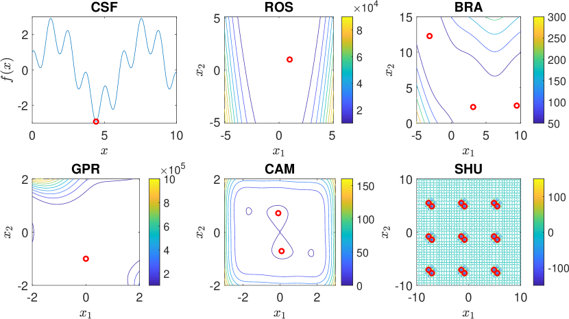
Figure 1: Plot of the 1D function CSF and contours of the 2D test functions. The red circles represent the global optima.

5 Benchmark Results

This section empirically shows that the proposed acquisition function performs as well as or better than the state-of-the-art methods reviewed in Section 2.2, using an extensive set of benchmark problems from the global optimization literature (Jones et al., 1993; Huyer and Neumaier, 1999). Figure 2 shows the log₁₀ distance in function space to the global optimum as a function of the objective function evaluations $n$. Each trace represents the average log₁₀ distance of a given algorithm over the 5 different initial design instantiations, and the error bars show the standard error of the mean for the whole spectrum of iteration numbers. For two of the problems, CAM and SHU, the Max-Value Entropy Search method did not reach the maximum budget $n_{\max}$ in the allowed computational time (2 weeks). In these cases the log₁₀ distance in function space is shown up to the latest iteration.

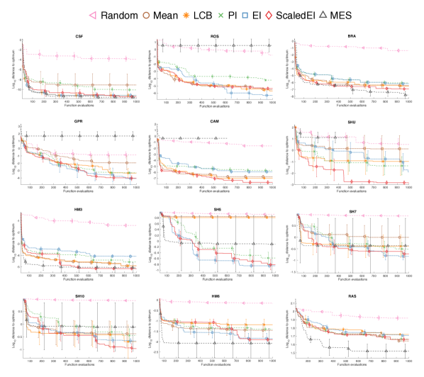
Figure 2: Comparison of the log₁₀ distances (in function space) to the global optimum. Each panel represents a given benchmark function. The traces show the average distance over the five design instantiations for the whole spectrum of iterations, while the error bars show plus or minus one standard error of the mean.

Table 2: Statistical test for the significance in the mean difference of the final log₁₀ distances. The ScaledEI acquisition function was tested against all remaining acquisition functions using a paired t-test with significance level 0.05. Codes: 0 indicates a non significant difference and 1 (-1) indicates that ScaledEI performed better (worse), i.e. it has a significantly lower (higher) average distance.

	ScaledEI vs
Test function	RND	MN	LCB	PI	EI	MES
CSF	1	0	0	1	0	0
ROS	1	0	0	1	0	1
BRA	1	0	0	0	1	0
GPR	1	0	0	0	0	1
CAM	1	0	0	1	1	1
SHU	1	0	0	0	0	1
HM3	1	0	0	0	1	0
SH5	1	1	1	0	0	0
SH7	1	0	0	0	0	0
SH10	1	0	0	0	0	0
HM6	1	0	0	1	0	0
RAS	1	0	0	0	0	0
Same	0%	92%	92%	67%	75%	67%
Better	100%	8%	8%	33%	25%	33%
Worse	0%	0%	0%	0%	0%	0%

The results in Figure 2 show that the RND policy is consistently outperformed by the improvement-based acquisition functions. In the 1D scenario (CSF) RND is the worst method, followed by MN, which has huge variation in the results. The best methods include improvement-based policies and MES, but there does not seem to be a significant difference between them. For most of the 2D functions (ROS, GPR, CAM, SHU) it appears that improvement-based policies outperform the information-theoretic one. In three of these functions the proposed ScaledEI outperforms all others. In the BRA function, MES seems to be the best, but by a small margin compared to the evident gap in the other 2D scenarios. In the 3D problem (HM3) EI is outperformed by the other methods, except for RND. However, the proposed method, ScaledEI, is the best, emphasizing the power of the proposed adjustment. Even in the 4D, 6D and 10D test functions the ScaledEI policy appears to be one of the most competitive methods, while its information-based competitor MES suffers from highly variable results.

In order to facilitate the interpretation of the results, we test in Table 2 the significance of the difference in means of the final log₁₀ distances for ScaledEI vs each of the remaining acquisition functions, using a paired t-test with significance level 0.05. We remark that the choice of performing a t-test on the log distances at the final iteration is only for summary purposes, and Figure 2 shows the full spectrum of performance scores for all function evaluations ranging from $n=100$ to $1000$. In most cases, the log distance curves are fairly flat between $300$ and $1000$, so the table presented here is representative of the majority of the choices of $n$. In general we would not get the true optimum at a high degree of accuracy with only $200$ function evaluations. Nevertheless, we have carried out the statistical hypothesis tests for $n=600$ and $n=200$ as well, and the results can be found in Tables 3 and 4. A score of 0 indicates that the null hypothesis of equal average log₁₀ distance is not rejected. Both 1 and -1 indicate the rejection of the null hypothesis, where a score of 1 indicates that the proposed method, ScaledEI, achieves a significant improvement, while a score of -1 shows that ScaledEI is significantly worse.

The proposed acquisition function ScaledEI consistently outperforms the naive RND policy. Compared with the established acquisition functions, ScaledEI nearly always achieves equal (67-92%) or significantly better (8-33%) performance, without being significantly outperformed by the competitors. One third of the times, ScaledEI is significantly better than PI and the information-theoretic competitor MES. This is corroborated in Figure 2, where for the benchmark functions ROS, GPR, CAM, SHU the information-theoretic policy does not come close to the minimum. Then follow EI and LCB, which are outperformed 25% and 8% of the times, and MN, which is, surprisingly, outperformed only 8% of the times. This finding provides reassurance for conservative BO strategies, as in Wang et al. (2013). However, the summary table based on hypothesis tests incurs a loss of information. From the t-test it is not evident that the MN policy suffers from huge variations in the results (see Figure 2). The fact that for some random number seeds MN performs well is due to the initial design generating a point near the global minimum by chance. Then, by emphasizing exploitation only, this point will be fine-tuned to the global optimum. ScaledEI never appears to be significantly worse than its competitors, and in particular the widely applied EI method. Our results suggest that the proposed acquisition function, ScaledEI, which combines high expected improvement with high confidence in the improvement being high, performs as well as or better than state-of-the-art acquisition functions. This makes ScaledEI a good default choice for standard BO applications.

Table 3: Statistical test for the significance in the mean difference of the log₁₀ distances at $\boldsymbol{n=600}$. The ScaledEI acquisition function was tested against all remaining acquisition functions using a paired t-test with significance level 0.05. Codes: 0 indicates a non significant difference and 1 (-1) indicates that ScaledEI performed better (worse), i.e. it has a significantly lower (higher) average distance.

	ScaledEI vs
Test function	RND	MN	LCB	PI	EI	MES
CSF	1	0	0	1	0	0
ROS	1	0	0	1	0	1
BRA	1	0	0	1	1	0
GPR	1	0	0	0	0	1
CAM	1	0	0	1	1	1
SHU	1	0	0	0	1	1
HM3	1	0	0	1	1	0
SH5	1	1	1	0	0	0
SH7	1	0	0	0	0	0
SH10	1	0	0	0	0	0
HM6	1	0	0	0	0	0
RAS	1	0	1	0	0	0
Same	0%	92%	83%	58%	67%	67%
Better	100%	8%	17%	42%	33%	33%
Worse	0%	0%	0%	0%	0%	0%

As already mentioned above, we would not expect the algorithms to fine-tune the returned optimum in only $n=200$ steps. However, for representational completeness we have carried out the statistical hypothesis tests for $n=600$ and $n=200$ nevertheless. These are shown in Tables 3 and 4 respectively.

Table 3 shows that at 600 iterations the results are consistent with Table 2, which uses the full budget of function evaluations. ScaledEI is always significantly better than RND, but only 8% of the times better than MN. Again, this is due to the random generation of an initial design point near a global minimum by chance, which is fine-tuned by focusing on exploitation only. However, this approach carries substantial variations in the results, and the success of the MN method depends entirely on the initial design choice, making it a non-optimal policy. For the remaining methods, ScaledEI is significantly better than each competitor 17-42% of the times, and in the remaining cases the methods are not significantly different. One third of the times it is better than the widely used EI method and the information-theoretic MES. Furthermore, ScaledEI is never significantly outperformed by its competitors, including MES. We finally report in Table 4 the same kind of test but stopping at $n=200$ iterations only. In this scenario, ScaledEI performed significantly better than PI and EI, 17% and 42% of the times respectively, while in the remaining cases the two were not significantly different. Comparing ScaledEI and the information theoretic strategy (MES), 50% of the time the two are not significantly different, but 33% ScaledEI is performing significantly better, and it is outperformed by MES in two benchmark functions only: HM3 and RAS.

As remarked in Section 2, different BO algorithms vary in the choice of the acquisition function. The proposed one, ScaledEI, was tested against literature methods on a set of 12 benchmark functions having different functional characteristics. According to the no-free-lunch theorem, we do not expect to see one method consistently outperforming all the remaining algorithms on all benchmark functions and for any arbitrary choice of function evaluations $n$. However, our results, shown in Figure 2 and Tables 2 to 4, suggest that ScaledEI tends to perform as well as or better than the alternative methods, and hence constitutes a powerful default choice for Bayesian optimization.

Table 4: Statistical test for the significance in the mean difference of the log₁₀ distances at $\boldsymbol{n=200}$. The ScaledEI acquisition function was tested against all remaining acquisition functions using a paired t-test with significance level 0.05. Codes: 0 indicates a non significant difference and 1 (-1) indicates that ScaledEI performed better (worse), i.e. it has a significantly lower (higher) average distance.

	ScaledEI vs
Test function	RND	MN	LCB	PI	EI	MES
CSF	1	0	0	0	0	0
ROS	1	0	0	1	1	1
BRA	1	0	0	1	1	0
GPR	0	0	0	0	0	1
CAM	1	0	0	0	1	1
SHU	0	0	0	0	1	1
HM3	1	0	0	0	1	-1
SH5	1	0	0	0	0	0
SH7	1	0	0	0	0	0
SH10	1	0	0	0	0	0
HM6	1	0	0	0	0	0
RAS	1	0	0	0	0	-1
Same	17%	100%	100%	83%	58%	50%
Better	83%	0%	0%	17%	42%	33%
Worse	0%	0%	0%	0%	0%	17%

6 Comparative Study with Standard Global Optimization Solvers

The goal of BO is to reduce the computational costs required to optimize an expensive-to-evaluate function $f$, by reducing the number of function evaluations. This section corroborates the claim by presenting a proof-of-concept study recording the number of function evaluations required to reach a log₁₀ distance to the true global optimum equal to $-6$. In this experiment we used the objective function CSF, shown in the top left panel of Figure 1, and compared ScaledEI with a range of algorithms widely used, for example, by applied mathematicians and engineers:

1. Genetic Algorithm (Goldberg, 1989; Conn et al., 1991, 1997);

2. Global Search (Ugray et al., 2007);

3. Simulated Annealing (Ingber, 1996);

4. Particle Swarm (Mezura-Montes and Coello Coello, 2011; Pedersen, 2010);

5. Multi Start (10 random starting points) (Ugray et al., 2007; Glover, 1998);

6. Pattern Search (Audet and Dennis, 2002; Abramson et al., 2009).

We used the implementation found in MATLAB’s Global Optimization Toolbox, with the default automatic settings for each algorithm. Each optimization was repeated 15 times, using different random number generator seeds.

Figure 3 shows, for each optimization algorithm, the average number of function evaluations (over the 15 random number seeds) required to reach a log₁₀ distance of $-6$, while the error bars show plus or minus one standard error of the mean.

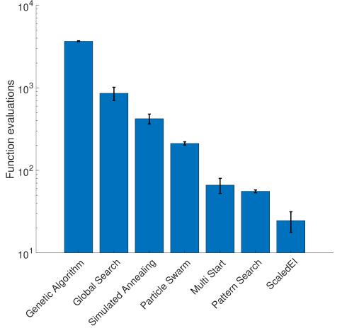
Figure 3: Number of function evaluations required to reach a log₁₀ distance to the true global optimum (in function space) equal to $\boldsymbol{-6}$.

The Genetic Algorithm, requiring between $10^{3}$ and $10^{4}$ function evaluations, is the least suitable algorithm for expensive objective functions. Then follow Global Search, which requires in the order of $10^{3}$ evaluations, Simulated Annealing and Particle Swarm, both requiring between $10^{2}$ and $10^{3}$ evaluations. The Multi Start and Pattern Search solvers rank as the most efficient ones, in terms of the number of function evaluations, but they are clearly outperformed by ScaledEI. This comes as no surprise as, by construction, BO algorithms use all the information available from previous function evaluations to internally maintain a surrogate model of the objective function and infer its geometric properties in order to recommend the next candidate point.

7 Application to In Silico Medicine

Chronic pulmonary arterial hypertension (PH), i.e. high blood pressure in the pulmonary circulation, is often referred to as a “silent killer” and is a disease of the small pulmonary arteries. It can lead to irreversible changes in the pulmonary vascular structure and function, increased pulmonary vascular resistance, and right ventricle hypertrophy leading to right heart failure (Allen et al., 2014; Rosenkranz and Preston, 2015).

For diagnosis and ongoing treatment and assessment, clinicians measure blood flow and pressure within the pulmonary arteries. As opposed to blood pressure in the systemic circulation, measured using a sphygmomanometer, blood pressure in the pulmonary circulation can only be measured using invasive techniques such as right heart catheterization. Invasive techniques can lead to complications (internal bleeding, severe pain, thrombosis, etc.), for that reason, it is desirable to predict the blood pressure indirectly based on quantities that can be measured non-invasively. Furthermore, data about healthy patients are not available due to ethical reasons. This section uses a partial differential equations (PDEs) model of the pressure and flow wave propagation in the pulmonary circulation under normal physiological and pathological conditions, introduced by Qureshi et al. (2014) and also studied by Noè et al. (2017). The goal is to use the novel ScaledEI Bayesian optimization algorithm introduced in (6) and the pulmonary circulation model cited above to infer indicators of pulmonary hypertension risk which could be used by clinicians to inform their diagnosis instead of taking invasive measurements.

The PDEs depend on various physiological parameters, related e.g. to blood vessel geometry, vessel stiffness and fluid dynamics. These parameters, which would give important insights into the status of a patient’s pulmonary circulatory system, can typically not be measured in vivo and hence need to be inferred indirectly from the observed blood flow and pressure distributions. In principle, this is straightforward. Under the assumption of a suitable noise model, the solutions of the PDEs define the likelihood of the data, and the parameters can then be inferred in a maximum likelihood sense. However, a closed-form solution of the maximum likelihood equations is not available, which calls for an iterative optimization procedure. Since a closed-form solution of the PDEs is not available either, each optimization step requires a numerical solution of the PDEs. This is computationally expensive, especially given that the likelihood function is typically multi-modal, and the optimization problem is NP-hard. Minimization of the residual sum of squares (negative log likelihood) hence calls for Bayesian optimization in order to reduce the computational costs of the inference. The estimated parameters of the PDEs will give clinicians insights into the patient-specific vessel structure that would not be obtainable in vivo such as vessel stiffnesses, a primary indicator of hypertension.

7.1 The Pulmonary Circulation Model

In the model of the pulmonary circulation by Qureshi et al. (2014), seven large arteries and four large veins are modelled explicitly, while the smaller vessels are represented by structured trees (Figure 4). A magnetic resonance imaging (MRI) based measurement of the right ventricular output provides the inlet flow for the system.

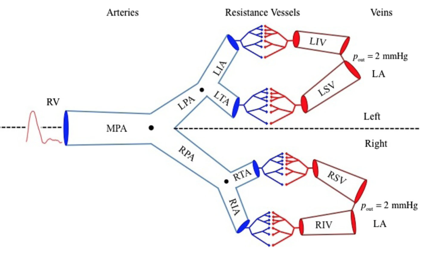
Figure 4: Schematic of the pulmonary circulation consisting of large arteries, arterioles, venules and large veins from Qureshi et al. (2014). Seven large arteries are considered in this model, i.e. the main pulmonary artery (MPA), the left (LPA) and right (RPA) pulmonary arteries, the left interlobular artery (LIA), the left trunk artery (LTA), the right interlobular artery (RIA), and the right trunk artery (RTA). The four terminal arteries LIA, LTA, RIA, and RTA are connected to four large veins, i.e. the left inferior vein (LIV), left superior vein (LSV), right inferior vein (RIV), and right superior vein (RSV), via structured trees of resistance vessels.

The large arteries and veins are modelled as tapered elastic tubes, and the geometries are based on measurements of proximal and distal radii and vessel lengths. The cross-sectional area averaged blood flow and pressure are predicted from a non-linear model based on the incompressible Navier–Stokes equations for a Newtonian fluid. The small arteries and veins are modelled as structured trees at each end of the terminal large arteries and veins to mimic the dynamics in the vascular beds. With a given parent vessel radius $r_{p}$, the daughter vessels are scaled linearly with radii $r_{d_{1}}=\alpha r_{p}$ and $r_{d_{2}}=\beta r_{p}$, where $\alpha$ and $\beta$ are the scaling factors. The vessels bifurcate until the radius of each terminal vessel is smaller than a given minimum $r_{\min}$. The radius relation at bifurcations is:

$$r_{p}^{\xi}=r_{d_{1}}^{\xi}+r_{d_{2}}^{\xi},\quad 2.33\leq\xi\leq 3.0,$$ (7)

where the exponent $\xi=2.33$ corresponds to laminar flow, $\xi=3.0$ corresponds to turbulent flow (Olufsen, 1999), $p$ represents the parent vessel, and $d_{1}$ and $d_{2}$ represent the daughter vessels. Given the area ratio $\eta=(r_{d_{1}}^{2}+r_{d_{2}}^{2})/{r_{p}^{2}}$ and the asymmetry ratio $\gamma=(r_{d_{2}}/r_{d_{1}})^{2}$, the scaling factors $\alpha$ and $\beta$ satisfy $\alpha=(1+\gamma^{\xi/2})^{-1/\xi}$ and $\beta=\alpha\sqrt{\gamma}$. The parameters, $\xi$, $\gamma$, $r_{\min}$ and a given root radius $r_{0}$, determine the size and density of the structured tree. The cross-sectional area averaged blood flow and pressure in these small arteries and veins are computed from the linearized incompressible axisymmetric Navier–Stokes equations (Qureshi et al., 2014).

For each large vessel, the pressure and flow are modelled as the solution of the one dimensional Navier–Stokes equation (Olufsen et al., 2012). It comprises two equations which ensure conservation of volume and momentum, and a third equation of state, relating pressure and cross-sectional area. Let $x$ denote the distance along a given vessel, $t$ represent time, $p(x,t)$ the pressure, $q(x,t)$ the volumetric flow along any given vessel, $A(x,t)$ the corresponding cross-sectional area, $\rho$ a constant representing the density of the blood, $\nu$ a constant representing kinematic viscosity, $\delta$ (constant) the boundary layer thickness, and $r(x,t)$ the radius of the given vessel. Conservation of volume and momentum is satisfied by:

$$\frac{\partial q}{\partial x}+\frac{\partial A}{\partial t}=0,\qquad\frac{\partial q}{\partial t}+\frac{\partial}{\partial x}\left(\frac{q^{2}}{A}\right)+\frac{A}{\rho}\frac{\partial p}{\partial x}=-\frac{2\pi\nu r}{\delta}\frac{q}{A}.$$ (8)

The constitutive law linking pressure and cross sectional area is given by:

$$p(x,t)-p_{0}=\frac{4}{3}\frac{Eh}{r_{0}}\left(1-\sqrt{\frac{A_{0}}{A}}\right),$$ (9)

where $p_{0}$ denotes the external pressure, $E$ is Young’s modulus, $h$ the vessel wall thickness and $r_{0}$ the vessel radius when $p(x,t)=p_{0}$. The unstressed vessel area is obtained as $A_{0}=\pi r_{0}^{2}$. The term $Eh/r_{0}$ in (9) describes the elastic properties of a vessel’s wall, and hence represents a parameter that controls the system compliance. This will be simply denoted by $f_{\mathrm{L}}$ in the large vessels and by $f_{\mathrm{S}}$ in the small vessels.

In the small vessels, similarly to the large ones, three equations determine the flow, pressure and area of each vessel in the structured tree. Olufsen et al. 2012 however, notice that in small vessels the nonlinear effects are small, effectively allowing for linearization of the constitutive equations. The full system of PDEs is presented in Qureshi et al. (2014), and its numerical solution, which depends on various physiological parameters, will henceforth be referred to as simulation. Figure 5 shows the simulated pressure (left) and flow (right) curves over time at three different locations in the main pulmonary artery (MPA).

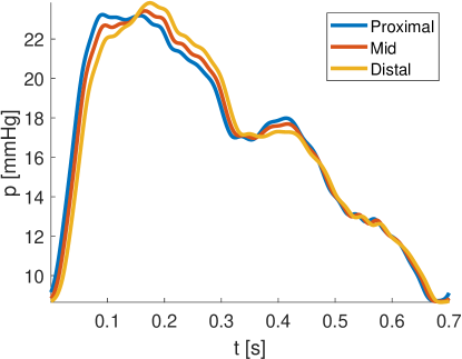
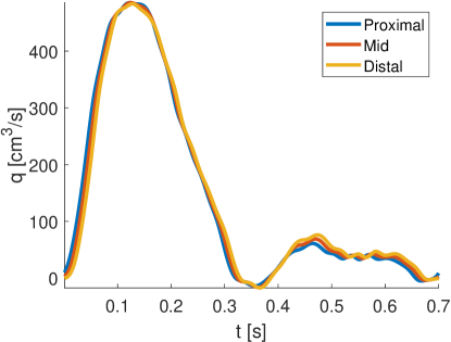
Figure 5: Simulated pressure (left) and flow (right) over time, at three different locations along the MPA.

Particular interest lies in the estimation of the parameter $\xi$, because low values are indicative of the clinically relevant problem of vascular rarefaction, which is a well-known finding in patients suffering from pulmonary hypertension, and represents the condition of having fewer blood vessels per tissue volume (Feihl et al., 2006). Estimation of $\xi$ is performed in the range $2.33\leq\xi\leq 3$. Other relevant parameters of interest for clinical diagnosis are the stiffness parameters in the large and small vessels, $f_{\mathrm{L}}$ and $f_{\mathrm{S}}$ respectively, with bounds $f_{\mathrm{L}}\in[1.33\times 10^{5},5.33\times 10^{5}]$ and $f_{\mathrm{S}}\in[2.66\times 10^{4},1.066\times 10^{5}]$ as in Noè et al. (2017). Increased vessel stiffness is a major cause of pulmonary hypertension. During systole, a compliant artery expands to accommodate for the inflow, while it recoils during diastole to promote forward flow. As the capacity of an artery is limited, the pressure increases during systole and is partially maintained during diastole by the rebounding of the expanded arterial walls. When the stiffness is increased, the cushioning function of the vessel is compromised, leading to a higher systolic and a lower diastolic pressure. All remaining model parameters are fixed to biologically relevant value from the literature as in Qureshi et al. (2014).

7.2 Bayesian Optimization with Hidden Constraints

Mathematical models often rely on simplifying assumptions about the underlying system. When these assumptions do not hold, the model can return a failure instead of a numerical simulation. In the considered model of the human pulmonary circulation, for some specific settings of the PDE parameters this is indeed the case. However, the regions in the parameters space that lead to failures are unknown a priori. A problem is said to contain hidden constraints if a requested function value may turn out not to be obtainable. This is different from the case where an output value is obtained but deemed not valid.

In this case the optimization of the function must be performed hand-in-hand with a sequential learning of the domain areas leading to numerical failures. This requires a modification of Algorithm 1, as in Gelbart et al. (2014). The idea is that, along with each function evaluation $y_{i}=f(\boldsymbol{x}_{i})$, we also keep track of the failure or success of the query in an auxiliary variable $h_{i}=h(\boldsymbol{x}_{i})$. The convention used in our work for the binary variable $h(\boldsymbol{x})$ is to take the value $1$ in case of a failure and $-1$ for a successful evaluation. Hence, we name $h\in\{-1,1\}$ the failure indicator. The initial design will consist of triples $(\boldsymbol{x}_{i},y_{i},h_{i})$ for $i=1,\dots,n_{\mathrm{init}}$. The next step consists in obtaining two GP models:

1. a GP model of the objective function, using the $(\boldsymbol{x}_{i},y_{i})$ pairs;

2. a GP model of the failures, using the $(\boldsymbol{x}_{i},h_{i})$ pairs.

Model (a) represents a standard GP regression as described in Section 2.1, while model (b) requires predicting the posterior class probabilities of $h$ for a new input $\boldsymbol{x}$, given a set of training data. For the GP classification with logit or probit link function, the class posterior probability is analytically intractable. Different approximations have been proposed in order to predict binary-valued outcomes, for example iterative procedures like Expectation Propagation (EP), Laplace approximation (LA) or the simpler label regression (LR) approach.

Following the experiments and recommendations of Kuss (2006), which suggest that label regression works surprisingly well in practice and with a lower error rate than the competing methods in high dimensions, we apply LR in order to build a model of the simulation failures, ignoring the binary nature of the variable $h$ in favor of a quicker runtime and a closed-form posterior. Any approximation involving extra iterative procedures could cause the modelling and point selection time to be higher than simply evaluating the objective function. In other words, we would spend more time in modelling the function rather than evaluating it. While this can be arguably acceptable for really expensive simulators, it would not be computationally optimal for the presented application. A discussion of the computational costs of the pulmonary circulation model under study can be found in Section 7.3.

Denote the failure indicator model as $h(\boldsymbol{x})\sim\mathsf{GP}(\hat{h}(\boldsymbol{x}),s_{h}(\boldsymbol{x},\boldsymbol{x}^{\prime}))$, obtained by applying the formulas summarized in Section 2.1 to the $\{(\boldsymbol{x}_{i},h_{i})\}$ data. By the marginalization property of GPs, at point $\boldsymbol{x}$ the random variable $h(\boldsymbol{x})$ follows a $\mathsf{N}(\hat{h}(\boldsymbol{x}),s_{h}^{2}(\boldsymbol{x}))$ distribution. As failures are labelled as $1$ and successful evaluations as $-1$, by taking the probability of the Gaussian random variable being less than $0$ we obtain an indication of the probability of a successful evaluation (no failure):

$$\mathbb{P}\{h(\boldsymbol{x})=-1\}=\Phi(0\mid\hat{h}(\boldsymbol{x}),s^{2}_{h}(\boldsymbol{x})).$$ (10)

This probability can then be used to weight the score that any acquisition function assigns to a point in the domain as follows (Gelbart et al., 2014):

$$a_{n}^{*}(\boldsymbol{x}) =a_{n}(\boldsymbol{x})\times\mathbb{P}\{h(\boldsymbol{x})=-1\}$$ (11)

$$=a_{n}(\boldsymbol{x})\times\Phi(0\mid\hat{h}(\boldsymbol{x}),s^{2}_{h}(\boldsymbol{x})).$$

We refer to $a_{n}^{*}(\boldsymbol{x})$ as the hidden-constraints-weighted acquisition function. The algorithm then proceeds normally by choosing the next query point as the point maximizing $a_{n}^{*}(\boldsymbol{x})$. A pseudocode summary can be found in Algorithm 2. From (11) we see that both models (a) and (b) are required in order to compute the hidden-constraints-weighted acquisition function at each iteration of the BO algorithm.

Algorithm 2 Bayesian optimization with hidden constraints.

1:  Inputs: Initial design and corresponding failure labels: $\mathcal{D}_{n_{\mathrm{init}}}=\{(\boldsymbol{x}_{i},y_{i},h_{i})\}_{i=1}^{n_{\mathrm{init}}}$ Budget of $n_{\mathrm{max}}$ function evaluations

1:  

2:  for $n=n_{\mathrm{init}}$ to $n_{\mathrm{max}}-1$ do

3:     Update the objective GP: $f(\boldsymbol{x})\mid\mathcal{D}_{n}\sim\mathsf{GP}(\hat{f}(\boldsymbol{x}),s(\boldsymbol{x},\boldsymbol{x}^{\prime}))$

4:     Update the failure GP: $h(\boldsymbol{x})\mid\mathcal{D}_{n}\sim\mathsf{GP}(\hat{h}(\boldsymbol{x}),s_{h}(\boldsymbol{x},\boldsymbol{x}^{\prime}))$

5:     Compute the acquisition function: $a_{n}^{*}(\boldsymbol{x})=a_{n}(\boldsymbol{x})\times\Phi(0\mid\hat{h}(\boldsymbol{x}),s_{h}^{2}(\boldsymbol{x}))$

6:     Solve the auxiliary optimization problem: $\boldsymbol{x}_{\mathrm{next}}=\operatornamewithlimits{argmax}_{\boldsymbol{x}\in\mathbb{X}}a_{n}^{*}(\boldsymbol{x})$

7:     Query $f$ at $\boldsymbol{x}_{\mathrm{next}}$ to obtain $y_{\mathrm{next}}$ and $h_{\mathrm{next}}$

8:     Augment data: $\mathcal{D}_{n+1}=\mathcal{D}_{n}\cup\{\boldsymbol{x}_{\mathrm{next}},y_{\mathrm{next}},h_{\mathrm{next}}\}$

9:  end for

9:  

10:  Return: Estimated minimum: $f_{\mathrm{min}}=\min(y_{1},\dots,y_{n_{\mathrm{max}}})$ Estimated point of minimum: $\boldsymbol{x}_{\mathrm{min}}=\operatornamewithlimits{argmin}(y_{1},\dots,y_{n_{\mathrm{max}}})$

At termination, the learned failure GP model can be used to obtain insights into the regions in the parameter domain leading to failure. For plotting purposes, in Figure 6 we show the probability of a successful evaluation (no failure), $\mathbb{P}\{h(\boldsymbol{x})=-1\}=\Phi(0\mid\hat{h}(\boldsymbol{x}),s^{2}_{h}(\boldsymbol{x}))$, for the 2D parameter space $\boldsymbol{x}=(f_{\mathrm{L}},\xi)^{\top}$. The figure shows how it is possible to have regions of failure inside a larger area of successful simulations.

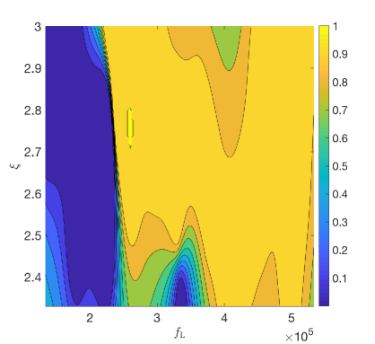
Figure 6: Learned probability of a successful simulation in the PDEs model of the human pulmonary circulation. A score near 1 indicates a high chance of a successful simulation, while a score near 0 indicates a high probability of failure.

7.3 Estimation of the Model Parameters

In the computational model of the pulmonary circulation, denoted by $\mathsf{m}$, a forward simulation for fixed parameters takes around 23 seconds of CPU time. The data collected by clinicians typically include pressure and flow measurements only from the midpoints of the 11 large vessels. In light of this, we refer to a simulation as the $22$-dimensional vector $\boldsymbol{y}=\mathsf{m}(\boldsymbol{q})$ containing pressure and flow measurements at the midpoint location of each of the 7 large arteries and 4 large veins, for a given vector of PDE parameters $\boldsymbol{q}$. Given the costs of a single function evaluation, parameter estimation comes at substantial computational demands as standard global optimization algorithms require a large number of forward simulations (for example see Figure 3). Motivated by real-time decision making, we want to reduce the computational time required to estimate the PDE parameters by keeping the number of function evaluations as low as possible. To do so, we tackle this problem by using Bayesian optimization with hidden constraints and the novel ScaledEI acquisition function introduced in (6).

Let $\boldsymbol{q}=(f_{\mathrm{L}},f_{\mathrm{S}},\xi)^{\top}$ denote the three parameters of relevance for the diagnosis of pulmonary hypertension. The simulated pressure and flow data $\boldsymbol{y}_{0}$ are obtained by a forward simulation of the computational model at the vector of parameters $\boldsymbol{q}_{0}=(2.6\times 10^{5},5\times 10^{4},2.76)^{\top}$, assumed to be the underlying truth, and the data are then corrupted by i.i.d. additive Gaussian noise with a signal-to-noise ratio (SNR) of 10db. Pretending that the true parameter vector $\boldsymbol{q}_{0}$ is unknown, interest lies in its estimation from the noisy observations $\boldsymbol{y}_{0}$. This is to present a proof-of-concept study carried out on simulated data, for which it is possible to assess the inference as the gold-standard is known, but with the objective to ultimately apply it to real data and move it into the clinic. For i.i.d. additive Gaussian noise, the residual sum of squares is proportional to the negative log likelihood. Hence, the objective function considered in this study is the squared L2 loss, or residual sum of squares, between a simulation $\mathsf{m}(\boldsymbol{q})$ and the data $\boldsymbol{y}_{0}$:

$$\ell(\boldsymbol{q})=\|\mathsf{m}(\boldsymbol{q})-\boldsymbol{y}_{0}\|^{2}.$$ (12)

Since each evaluation of the squared loss $\ell$ involves an expensive forward simulation from the PDE model $\mathsf{m}(\boldsymbol{q})$, also each evaluation of $\ell$ will be expensive. We estimate the parameters $\boldsymbol{q}=(f_{\mathrm{L}},f_{\mathrm{S}},\xi)^{\top}$ by minimizing the squared loss using Bayesian optimization with hidden constraints and the ScaledEI acquisition function, with the following notational correspondence in Algorithm 2:

• Objective function: $f(\boldsymbol{x})\equiv\ell(\boldsymbol{q})$;

• Input: $\boldsymbol{x}_{i}\equiv\boldsymbol{q}_{i}$;

• Output: $y_{i}\equiv\ell_{i}$.

In this experiment we set a priori the maximum budget of function evaluations to $n_{\mathrm{max}}=500$. We repeated the optimization of $\ell$ using fifteen different random number seeds. Let $\ell_{\min}=\min(\ell_{1},\dots,\ell_{n})$ denote the minimum observed objective (current best function value) at iteration $n$.

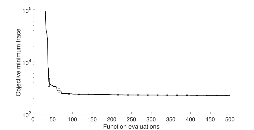
Figure 7: Optimization of the squared L2 loss for the pulmonary circulation model using the ScaledEI BO algorithm. The plot shows the minimum observed squared L2 loss trace, averaged over the 15 Latin hypercube design instantiations, plus or minus one standard error, as function of the number of function evaluations.

Figure 7 shows the average objective minimum trace, over the fifteen designs, as function of the number of function evaluations $n$ $(n=1,\dots,n_{\mathrm{max}})$. The error bars represent plus or minus one standard error of the mean. When the maximum budget of function evaluations is exceeded, the BO algorithm stops by returning the estimated objective minimum, $\ell_{\min}$, and the point $\boldsymbol{q}_{\min}$ at which the minimum is attained. The vector $\boldsymbol{q}_{\min}$ represents the estimate of the true but unknown $\boldsymbol{q}_{0}$.

Table 5: The PDE parameters underlying the simulated data (Truth) and the estimated parameters (Estimate). Mean and standard error over the 15 design instantiations.

	Truth	Estimate $(n=500)$		Estimate $(n=100)$
		Mean	Std. Err.	Mean	Std. Err.
$f_{\mathrm{L}}$	$2.6\times 10^{5}$	$2.6005\times 10^{5}$	$189.3129$	$2.599\times 10^{5}$	$286.5552$
$f_{\mathrm{S}}$	$50000$	$50003$	$35.0108$	$50038$	$55.9675$
$\xi$	$2.76$	$2.7603$	$0.0002$	$2.76$	$0.0004$

Table 5 shows the average and standard error, over the 15 repetitions, of the estimated point of minimum $\boldsymbol{q}_{\min}$ at iteration $n=n_{\mathrm{max}}$, next to the truth $\boldsymbol{q}_{0}$ used to generated the data. Considering that the data were corrupted by noise, the estimation (Mean) is accurate, and with reasonably small uncertainty (Std. Err.) given the scale of each parameter. Furthermore, each element of the true parameter vector $\boldsymbol{q}_{0}$ lies inside the 95% confidence interval obtained as the Mean plus or minus two Std. Err. in Table 5. We notice that the curve in Figure 7 is approximately flat after 100 function evaluations. For this reason, we could have effectively stopped at approximately between 100 and 200 iterations, without a substantial loss in accuracy, while reducing the overall computational time from 3 hours to less than 1 hour. In Table 5 we also report the estimated parameters stopping at $n=100$ function evaluations only, where one run of the optimization takes approximately 30 minutes, compared to the 3 hours required for $n=500$. These timings can be used for in-clinic decision support systems of practical relevance. However, for a standard optimization algorithm requiring, for example, $10^{4}$ function evaluations, one run of the algorithm would have taken approximately 3 days, making traditional algorithms not suitable for in-clinic applications.

8 Conclusions

We have proposed a new acquisition function for Bayesian optimization (BO) which falls into the class of improvement-based policies (class 2), summarized in Section 2.2. It is based on a random variable, called Improvement, defined in (2), which quantifies the improvement on the incumbent optimum. We have discussed that the established Expected Improvement acquisition function (4) does not account for the uncertainty in the Improvement random variable, which conveys information about our confidence in its value. We have overcome this problem by deriving the variance of Improvement in (5) and using it to derive a new acquisition function, referred to as ScaledEI, which is the ratio of the Expected Improvement and the standard deviation of Improvement, see (6). The proposed acquisition function accounts for another source of uncertainty, and the scaling factor plays a role in both exploitational and explorational moves. By selecting the point that maximizes the ScaledEI policy we effectively select a point for which we expect, on average, a high degree of improvement at high confidence.

We have evaluated the performance of the proposed acquisition function on an extensive set of benchmark problems from the global optimization literature. The test suite includes problems of different dimensionality, varying from 1D to 10D, having multiple local minima and, additionally, symmetries corresponding to multiple equivalent global minima.

The performance was evaluated in terms of the log₁₀ distance (in function space) to the global optimum. The results indicate that ScaledEI tends to perform as well as or better than the representative set of state-of-the-art methods from the BO literature included in our study. This suggests that by adopting a new search strategy that explicitly combines the expected improvement with its estimated uncertainty, we obtain a better trade-off between exploration and exploitation. The result is a new competitive search strategy that does not only compare favourably with other improvement-based alternatives (class 2), but also with optimistic (class 1) and information-theoretic (class 3) strategies.

We have then shown a proof-of-concept study that confirms the reduction in the number of function evaluations required to optimize the CSF function. The proposed ScaledEI algorithm was compared to a set of widely used global optimization solvers, by reporting the number of function evaluations required to reach a given tolerance on the $f$ value. The plot in Figure 3 confirms that Bayesian optimization with the proposed ScaledEI acquisition function has indeed the lowest number of function evaluations, since it uses a surrogate model of the objective function to inform the next evaluation.

Our final contribution was a proof-of-concept study based on a PDE fluid dynamics model of the human pulmonary circulation, which is potentially relevant to precision medicine and non-invasive real-time diagnosis. The aim was to use the PDE model in order to give clinicians three clear indicators of pulmonary hypertension, without going through the invasive procedure of right heart catheterization. The three indicators (large vessels stiffness, small vessels stiffness and density of the structured tree, representing vascular rarefaction) are derived from the parameters of the constitutive equations of the soft tissues, which give pathophysiological insights that are very difficult to obtain in vivo. We have shown how to estimate the three parameters using the proposed ScaledEI method, introduced in Section 3. In particular, the estimates were obtained in a time frame that is suitable for in-clinic diagnosis and prognosis. As seen from Figure 3, this goal would be more challenging to achieve with conventional non-Bayesian optimization routines. Hence, our combination of the new ScaledEI method with the fledgling fluid dynamics model of the human pulmonary blood circulation system is an important first stepping stone on the pathway to an autonomous in silico clinical decision support system.

Appendix A Appendix

Let $f(\boldsymbol{x})\sim\mathsf{GP}(m(\boldsymbol{x}),k(\boldsymbol{x},\boldsymbol{x}^{\prime}))$ be the GP prior on the objective function. We recall that given data $\mathcal{D}_{n}=\{(\boldsymbol{x}_{1},y_{1}),\dots,(\boldsymbol{x}_{n},y_{n})\}$ the predictive distribution at $\boldsymbol{x}$ is the marginal GP $f(\boldsymbol{x})\mid\mathcal{D}_{n}\sim\mathsf{N}(\hat{f}(\boldsymbol{x}),s^{2}(\boldsymbol{x}))$. By standardization, $z(\boldsymbol{x})=\{f(\boldsymbol{x})-\hat{f}(\boldsymbol{x})\}/s(\boldsymbol{x})\sim\mathsf{N}(0,1)$. Define the Improvement at $\boldsymbol{x}$ as the random variable $I(\boldsymbol{x})=\max\{f_{\mathrm{min}}-f(\boldsymbol{x}),0\}$, where $f_{\mathrm{min}}=\min(y_{1},\dots,y_{n})$ denotes the current best function value at iteration $n$.

A.1 Derivatives of Gaussian pdfs

Let $\phi(z)=(\sqrt{2\pi})^{-1}\exp(-z^{2}/2)$ be the standard Gaussian pdf. Then,

$$\phi^{\prime}(z)=\frac{\operatorname{d}}{\operatorname{d}z}\phi(z)=\phi(z)\times\left(-\frac{1}{2}\times 2z\right)=-z\phi(z).$$ (13)

The second derivative of the standard Gaussian pdf is:

$$\phi^{\prime\prime}(z) =\frac{\operatorname{d}}{\operatorname{d}z}\phi^{\prime}(z)$$

$$=\frac{\operatorname{d}}{\operatorname{d}z}\left\{-z\phi(z)\right\}$$ (14)

$$=-\phi(z)+(-z)(-z\phi(z))$$

$$=(z^{2}-1)\phi(z).$$

A.2 Derivation of the Probability of Improvement

The Probability of Improvement (PI) is the probability of the event $\{I(\boldsymbol{x})>0\}$ or, equivalently, $\{f(\boldsymbol{x})<f_{\mathrm{min}}\}$:

$$\mathrm{PI}(\boldsymbol{x}) =\mathbb{P}\{I(\boldsymbol{x})>0\}$$

$$=\mathbb{E}1_{\{f(\boldsymbol{x})<f_{\mathrm{min}}\}}$$

$$=\mathbb{P}\{f(\boldsymbol{x})<f_{\mathrm{min}}\}$$

$$=\mathbb{P}\left\{\frac{f(\boldsymbol{x})-\hat{f}(\boldsymbol{x})}{s(\boldsymbol{x})}<\frac{f_{\mathrm{min}}-\hat{f}(\boldsymbol{x})}{s(\boldsymbol{x})}\right\}$$

$$=\int_{-\infty}^{\frac{f_{\mathrm{min}}-\hat{f}(\boldsymbol{x})}{s(\boldsymbol{x})}}\phi(z)\operatorname{d}z$$

$$=\Phi\left(\frac{f_{\mathrm{min}}-\hat{f}(\boldsymbol{x})}{s(\boldsymbol{x})}\right),$$

where $\phi(x\mid\mu,\sigma^{2})$ and $\Phi(x\mid\mu,\sigma^{2})$ represent the pdf and cdf of a $\mathsf{N}(\mu,\sigma^{2})$ distribution evaluated at $x$ respectively. When $\mu=0$ and $\sigma^{2}=1$ we will simply write $\phi(x)$ and $\Phi(x)$ for brevity.

A.3 Derivation of the Expected Improvement

Define $u=\{f_{\mathrm{min}}-\hat{f}(\boldsymbol{x})\}/s(\boldsymbol{x})$. The expected value of the random variable $I(\boldsymbol{x})$ is the Expected Improvement (EI) acquisition function:

$$\mathrm{EI}(\boldsymbol{x}) =\mathbb{E}[I(\boldsymbol{x})]$$

$$=\mathbb{E}[\max\{f_{\mathrm{min}}-f(\boldsymbol{x}),0\}]$$

$$=\mathbb{E}\left[\{f_{\mathrm{min}}-f(\boldsymbol{x})\}1_{\{f(\boldsymbol{x})<f_{\mathrm{min}}\}}\right]$$

$$=\int_{-\infty}^{\infty}\{f_{\mathrm{min}}-y\}1_{\{y<f_{\mathrm{min}}\}}\phi(y\mid\hat{f}(\boldsymbol{x}),s^{2}(\boldsymbol{x}))\operatorname{d}y$$

$$=\int_{-\infty}^{f_{\mathrm{min}}}\{f_{\mathrm{min}}-y\}\phi(y\mid\hat{f}(\boldsymbol{x}),s^{2}(\boldsymbol{x}))\operatorname{d}y$$

$$=\int_{-\infty}^{u}\{f_{\mathrm{min}}-(\hat{f}(\boldsymbol{x})+s(\boldsymbol{x})z)\}\phi(z)\operatorname{d}z$$

$$=\int_{-\infty}^{u}\{f_{\mathrm{min}}-\hat{f}(\boldsymbol{x})-s(\boldsymbol{x})z\}\phi(z)\operatorname{d}z$$

$$=\{f_{\mathrm{min}}-\hat{f}(\boldsymbol{x})\}\int_{-\infty}^{u}\phi(z)\operatorname{d}z-s(\boldsymbol{x})\int_{-\infty}^{u}z\phi(z)\operatorname{d}z$$

$$=\{f_{\mathrm{min}}-\hat{f}(\boldsymbol{x})\}\Phi\left(u\right)+s(\boldsymbol{x})\phi\left(u\right)$$

$$=s(\boldsymbol{x})\left\{u\Phi(u)+\phi(u)\right\}.$$

A.4 Matérn 5/2 kernel

This section presents similar results to Section 5, but using a Gaussian process with the ARD Matérn 5/2 kernel. The only exception is represented by the MES policy, whose code, provided by Wang and Jegelka (2017), only allows for the ARD Squared Exponential kernel. Figure 8 shows the full spectrum of log₁₀ distances (in function space) to the global optimum, for all function evaluations ranging from $n=100$ to $1000$.

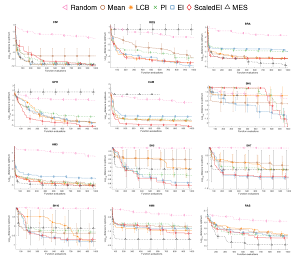
Figure 8: Comparison of the log₁₀ distances (in function space) to the global optimum. Each panel represents a given benchmark function. The traces show the average distance over the five design instantiations for the whole spectrum of iterations, while the error bars show plus or minus one standard error of the mean. These results use the ARD Matérn 5/2 kernel.

Tables 6, 7 and 8 test the significance of the difference in means of the log₁₀ distances at $n=1000,600,200$ respectively, for ScaledEI vs each of the remaining acquisition functions, using a paired t-test with significance level 0.05. Table 6 shows that ScaledEI always outperforms the simple RND policy, and often performs as well as (50-83%) or significantly better (17-50%) than the competing algorithms, with only one exception. ScaledEI is half of the time better than PI, followed by the information theoretic competitor MES, where ScaledEI performs significantly better 33% of the times. Then follow LCB and EI, both outperformed 25% of the times and finally the conservative MN policy, outperformed only 17% of the times. Due to the information loss inherent in reducing an entire graph to a single number, the huge variations in the results of MN get lost, but they are clear in Figure 8. By chance a point in the initial Latin hypercube design can be near the global optimum, and this will be fine-tuned because of the excessive exploitative strategy. ScaledEI appears to be worse than EI in only one test function. By inspecting in Figure 8 the trace of the log₁₀ distance for that function, SH10, we see that both algorithms are among the best performing methods, and the difference, even if significant, is marginal in absolute terms. Similar conclusions can be obtained from Tables 7 and 8.

We now compare Table 6, obtained using the ARD Matérn 5/2 kernel and Table 2, for the ARD Squared Exponential. ScaledEI performed always significantly better than the RND policy. Using the Squared Exponential kernel, ScaledEI is only once significantly better than MN while this happens twice using the Matérn kernel. For the Squared Exponential kernel, the ScaledEI method has a significantly better performance in only one of the benchmark functions, compared to LCB, while in the Matérn one this happens three times. Using the Matérn kernel, half of the time ScaledEI is better than PI, while using the infinitely-differentiable kernel, this happens only one third of the times. The comparison with EI is of particular interest. The column of t-test results are the same, apart from one function: SH10. Using the Squared Exponential kernel, there is not significant difference between ScaledEI and EI, while for the Matérn one the conclusion is that ScaledEI performed significantly worse. For both kernels, ScaledEI is significantly better than EI 25% of the times. We recall that the code of MES is only available for the Squared Exponential kernel. ScaledEI using either a Squared Exponential or Matérn 5/2 kernel is 33% of the times significantly better then MES with Squared Exponential kernel, and the remaining 67% of the times they are not significantly different.

Overall, 81% of the hypothesis test labels in Tables 2 to 4 versus Tables 6 to 8 agree between the two kernels, while in 19% of the cases they are different. This suggests that the two kernels lead to similar results.

Table 6: Statistical test for the significance in the mean difference of the final log₁₀ distances. The ScaledEI acquisition function was tested against all remaining acquisition functions using a paired t-test with significance level 0.05. Codes: 0 indicates a non significant difference and 1 (-1) indicates that ScaledEI performed better (worse), i.e. it has a significantly lower (higher) average distance. These results use the ARD Matérn 5/2 kernel.

	ScaledEI vs
Test function	RND	MN	LCB	PI	EI	MES
CSF	1	0	0	0	0	0
ROS	1	0	0	0	0	1
BRA	1	0	0	1	1	0
GPR	1	0	1	1	0	1
CAM	1	1	1	1	1	1
SHU	1	0	1	0	0	1
HM3	1	0	0	0	1	0
SH5	1	1	0	1	0	0
SH7	1	0	0	1	0	0
SH10	1	0	0	1	-1	0
HM6	1	0	0	0	0	0
RAS	1	0	0	0	0	0
Same	0%	83%	75%	50%	67%	67%
Better	100%	17%	25%	50%	25%	33%
Worse	0%	0%	0%	0%	8%	0%

Table 7: Statistical test for the significance in the mean difference of the log₁₀ distances at $\boldsymbol{n=600}$. The ScaledEI acquisition function was tested against all remaining acquisition functions using a paired t-test with significance level 0.05. Codes: 0 indicates a non significant difference and 1 (-1) indicates that ScaledEI performed better (worse), i.e. it has a significantly lower (higher) average distance. These results use the ARD Matérn 5/2 kernel.

	ScaledEI vs
Test function	RND	MN	LCB	PI	EI	MES
CSF	1	0	0	0	0	0
ROS	1	0	0	1	0	1
BRA	1	0	0	1	1	0
GPR	1	0	0	0	0	1
CAM	1	1	1	1	1	1
SHU	-1	0	0	0	0	0
HM3	1	0	0	0	1	0
SH5	1	0	0	0	0	0
SH7	1	0	0	0	0	0
SH10	1	0	0	1	0	0
HM6	1	0	0	0	0	0
RAS	1	0	0	0	0	0
Same	0%	92%	92%	67%	75%	75%
Better	92%	8%	8%	33%	25%	25%
Worse	8%	0%	0%	0%	0%	0%

Table 8: Statistical test for the significance in the mean difference of the log₁₀ distances at $\boldsymbol{n=200}$. The ScaledEI acquisition function was tested against all remaining acquisition functions using a paired t-test with significance level 0.05. Codes: 0 indicates a non significant difference and 1 (-1) indicates that ScaledEI performed better (worse), i.e. it has a significantly lower (higher) average distance. These results use the ARD Matérn 5/2 kernel.

	ScaledEI vs
Test function	RND	MN	LCB	PI	EI	MES
CSF	1	0	-1	0	-1	-1
ROS	1	1	0	1	0	1
BRA	1	1	1	1	1	0
GPR	1	0	1	0	0	1
CAM	1	1	1	1	1	1
SHU	0	0	0	0	0	0
HM3	1	0	0	0	1	0
SH5	1	0	0	0	0	0
SH7	1	0	0	0	0	0
SH10	1	0	0	0	0	0
HM6	1	0	0	0	0	0
RAS	1	0	0	0	0	0
Same	8%	75%	67%	75%	67%	67%
Better	92%	25%	25%	25%	25%	25%
Worse	0%	0%	8%	0%	8%	8%

References

- Abramson et al. (2009) Abramson MA, Audet C, Dennis JE, Digabel SL (2009) OrthoMADS: A Deterministic MADS Instance with Orthogonal Directions. SIAM Journal on Optimization DOI 10.1137/080716980, arXiv:0904.1950
- Allen et al. (2014) Allen RP, Schelegle ES, Bennett SH (2014) Diverse forms of pulmonary hypertension remodel the arterial tree to a high shear phenotype. American journal of physiology Heart and circulatory physiology 307(3):H405–17, DOI 10.1152/ajpheart.00144.2014
- Audet and Dennis (2002) Audet C, Dennis JE (2002) Analysis of Generalized Pattern Searches. SIAM Journal on Optimization DOI 10.1137/S1052623400378742
- Bergstra and Bengio (2012) Bergstra J, Bengio Y (2012) Random Search for Hyper-Parameter Optimization. Journal of Machine Learning Research 13(Feb):281–305
- Bergstra et al. (2011) Bergstra JS, Bardenet R, Bengio Y, Kégl B (2011) Algorithms for Hyper-Parameter Optimization. In: Proceedings of the 24th International Conference on Neural Information Processing Systems (NIPS), pp 2546–2554, DOI 2012arXiv1206.2944S, 1206.2944
- Calandra et al. (2016) Calandra R, Seyfarth A, Peters J, Deisenroth MP (2016) Bayesian optimization for learning gaits under uncertainty. Annals of Mathematics and Artificial Intelligence 76(1-2):5–23, DOI 10.1007/s10472-015-9463-9
- Conn et al. (1991) Conn AR, Gould NIM, Toint P (1991) A Globally Convergent Augmented Lagrangian Algorithm for Optimization with General Constraints and Simple Bounds. SIAM Journal on Numerical Analysis 28(2):545–572, DOI 10.1137/0728030
- Conn et al. (1997) Conn AR, Gould N, Toint P (1997) A globally convergent Lagrangian barrier algorithm for optimization with general inequality constraints and simple bounds. Mathematics of Computation DOI 10.1137/0728030
- Cox and John (1997) Cox DD, John S (1997) SDO: A Statistical Method for Global Optimization. In: Alexandrov NM, Hussaini MY (eds) Multidisciplinary Design Optimization: State of the Art, pp 315–329
- Feihl et al. (2006) Feihl F, Liaudet L, Waeber B, Levy BI (2006) Hypertension: A Disease of the Microcirculation? Hypertension 48(6):1012–1017, DOI 10.1161/01.HYP.0000249510.20326.72
- Garnett et al. (2010) Garnett R, Osborne MA, Roberts SJ (2010) Bayesian optimization for sensor set selection. In: Proceedings of the 9th ACM/IEEE International Conference on Information Processing in Sensor Networks (IPSN), ACM Press, New York, New York, USA, pp 209–219, DOI 10.1145/1791212.1791238
- Gelbart et al. (2014) Gelbart MA, Snoek J, Adams RP (2014) Bayesian optimization with unknown constraints. In: UAI’14 Proceedings of the Thirtieth Conference on Uncertainty in Artificial Intelligence, AUAI Press, Quebec City, Quebec, Canada, pp 250–259
- Glover (1998) Glover F (1998) A template for scatter search and path relinking. Springer, Berlin, Heidelberg, pp 1–51, DOI 10.1007/BFb0026589
- Goldberg (1989) Goldberg DE (1989) Genetic algorithms in search, optimization, and machine learning. Addison-Wesley Longman Publishing Co., Inc.
- Hennig and Schuler (2012) Hennig P, Schuler CJ (2012) Entropy Search for Information-Efficient Global Optimization. Journal of Machine Learning Research 13(Jun):1809–1837
- Hernández-Lobato et al. (2014) Hernández-Lobato JM, Hoffman MW, Ghahramani Z (2014) Predictive Entropy Search for Efficient Global Optimization of Black-box Functions. In: Proceedings of the 27th International Conference on Neural Information Processing Systems (NIPS), MIT Press, Montreal, Canada, pp 918–926
- Hutter et al. (2011) Hutter F, Hoos HH, Leyton-Brown K (2011) Sequential Model-Based Optimization for General Algorithm Configuration. In: Lecture Notes in Computer Science (including subseries Lecture Notes in Artificial Intelligence and Lecture Notes in Bioinformatics), vol 6683 LNCS, Springer, Berlin, Heidelberg, pp 507–523, DOI 10.1007/978-3-642-25566-3˙40
- Huyer and Neumaier (1999) Huyer W, Neumaier A (1999) Global Optimization by Multilevel Coordinate Search. Journal of Global Optimization 14(4):331–355, DOI 10.1023/A:1008382309369
- Ingber (1996) Ingber L (1996) Adaptive simulated annealing (ASA): Lessons learned. Control and Cybernetics DOI 10.1.1.15.2777, 0001018
- Jones et al. (1993) Jones DR, Perttunen CD, Stuckman BE (1993) Lipschitzian optimization without the Lipschitz constant. Journal of Optimization Theory and Applications 79(1):157–181, DOI 10.1007/BF00941892
- Jones et al. (1998) Jones DR, Schonlau M, Welch WJ (1998) Efficient Global Optimization of Expensive Black-Box Functions. Journal of Global Optimization 13(4):455–492, DOI 10.1023/A:1008306431147
- Kotthoff et al. (2017) Kotthoff L, Thornton C, Hoos HH, Hutter F, Leyton-Brown K (2017) Auto-WEKA 2.0: Automatic model selection and hyperparameter optimization in WEKA. Journal of Machine Learning Research 18(25):1–5
- Kushner (1964) Kushner HJ (1964) A New Method of Locating the Maximum Point of an Arbitrary Multipeak Curve in the Presence of Noise. Journal of Basic Engineering 86(1):97–106, DOI 10.1115/1.3653121
- Kuss (2006) Kuss M (2006) Gaussian Process Models for Robust Regression, Classification, and Reinforcement Learning. PhD thesis, Technische Universität Darmstadt, Darmstadt, Germany
- Lizotte et al. (2007) Lizotte D, Wang T, Bowling M, Schuurmans D (2007) Automatic gait optimization with Gaussian process regression. In: IJCAI International Joint Conference on Artificial Intelligence, pp 944–949
- Locatelli and Schoen (2013) Locatelli M, Schoen F (2013) Global optimization: theory, algorithms, and applications. Society for Industrial and Applied Mathematics (SIAM)
- Mezura-Montes and Coello Coello (2011) Mezura-Montes E, Coello Coello CA (2011) Constraint-handling in nature-inspired numerical optimization: Past, present and future. DOI 10.1016/j.swevo.2011.10.001
- Mockus (1975) Mockus J (1975) On Bayesian Methods for Seeking the Extremum. In: Lecture Notes in Computer Science (LNCS), vol 27, pp 400–404, DOI 10.1007/3-540-07165-2˙55, 1011.1669
- Mockus (1977) Mockus J (1977) On Bayesian Methods for Seeking the Extremum and their Application. In: IFIP Congress, pp 195–200
- Mockus (1989) Mockus J (1989) Bayesian Approach to Global Optimization, Mathematics and Its Applications, vol 37. Springer Netherlands, Dordrecht, DOI 10.1007/978-94-009-0909-0
- Noè et al. (2017) Noè U, Chen W, Filippone M, Hill N, Husmeier D (2017) Inference in a Partial Differential Equations Model of Pulmonary Arterial and Venous Blood Circulation Using Statistical Emulation. In: Computational Intelligence Methods for Bioinformatics and Biostatistics, Springer, Cham, Switzerland, pp 184–198, DOI 10.1007/978-3-319-67834-4˙15
- Olufsen (1999) Olufsen MS (1999) Structured tree outflow condition for blood flow in larger systemic arteries. American Journal of Physiology-Heart and Circulatory Physiology 276(1):H257–H268, DOI 10.1152/ajpheart.1999.276.1.H257
- Olufsen et al. (2012) Olufsen MS, Hill NA, Vaughan GDA, Sainsbury C, Johnson M (2012) Rarefaction and blood pressure in systemic and pulmonary arteries. Journal of fluid mechanics 705:280–305, DOI 10.1017/jfm.2012.220
- Pedersen (2010) Pedersen MEH (2010) Good Parameters for Particle Swarm Optimization. Technical Report HL1001
- Qureshi et al. (2014) Qureshi MU, Vaughan GDA, Sainsbury C, Johnson M, Peskin CS, Olufsen MS, Hill NA (2014) Numerical simulation of blood flow and pressure drop in the pulmonary arterial and venous circulation. Biomechanics and Modeling in Mechanobiology 13(5):1137–1154, DOI 10.1007/s10237-014-0563-y, NIHMS150003
- Rasmussen and Williams (2006) Rasmussen CE, Williams CKI (2006) Gaussian processes for machine learning. MIT Press
- Rosenkranz and Preston (2015) Rosenkranz S, Preston IR (2015) Right heart catheterisation: best practice and pitfalls in pulmonary hypertension. European Respiratory Review 24(138):642–652, DOI 10.1183/16000617.0062-2015
- Shahriari et al. (2016) Shahriari B, Swersky K, Wang Z, Adams RP, de Freitas N (2016) Taking the Human Out of the Loop: A Review of Bayesian Optimization. Proceedings of the IEEE 104(1):148–175, DOI 10.1109/JPROC.2015.2494218
- Snoek et al. (2012) Snoek J, Larochelle H, Adams RP (2012) Practical Bayesian Optimization of Machine Learning Algorithms. In: Proceedings of the 25th International Conference on Neural Information Processing Systems (NIPS), Curran Associates, Inc., pp 2951–2959
- Srinivas et al. (2012) Srinivas N, Krause A, Kakade SM, Seeger MW (2012) Information-Theoretic Regret Bounds for Gaussian Process Optimization in the Bandit Setting. IEEE Transactions on Information Theory 58(5):3250–3265, DOI 10.1109/TIT.2011.2182033
- Turner and Rasmussen (2012) Turner R, Rasmussen CE (2012) Model based learning of sigma points in unscented Kalman filtering. Neurocomputing 80:47–53, DOI 10.1016/J.NEUCOM.2011.07.029
- Ugray et al. (2007) Ugray Z, Lasdon L, Plummer J, Glover F, Kelly J, Martí R (2007) Scatter Search and Local NLP Solvers: A Multistart Framework for Global Optimization. INFORMS Journal on Computing 19(3):328–340, DOI 10.1287/ijoc.1060.0175
- Wang and Jegelka (2017) Wang Z, Jegelka S (2017) Max-value Entropy Search for Efficient Bayesian Optimization. In: Proceedings of the 34th International Conference on Machine Learning (PMLR), pp 3627–3635
- Wang et al. (2013) Wang Z, Mohamed S, Freitas N (2013) Adaptive Hamiltonian and Riemann Manifold Monte Carlo Samplers. In: Dasgupta S, McAllester D (eds) Proceedings of the 30th International Conference on Machine Learning (PMLR), PMLR, Atlanta, Georgia, USA, vol 28, pp 1462–1470