Spectral solution of load flow equations

Abstract

The load-flow equations are the main tool to operate and plan electrical networks. For transmission or distribution networks these equations can be simplified into a linear system involving the graph Laplacian and the power input vector. Decomposing the power input vector on the basis of the eigenvectors of the graph Laplacian, we solve this singular linear system. This spectral approach gives a new geometric view of the network and power vector. The power in the lines is then given as a sum of terms depending on each eigenvalue and eigenvector. We analyze the effects of these two components and show the important role played by localized eigenvectors. This spectral formulation yields a Parseval-like relation for the $L_{2}$ norm of the power in the lines. Using this relation as a guide, we propose to consider only the first few eigenvectors to approximate the power in the lines. Numerical results on IEEE cases support this approach which was also validated by analyzing chains and grids.

1 Introduction

The electrical grid is one of the major engineering achievements of the 20th century. Typically, it involves high voltage transmission lines connecting large generators and power sub-stations. The distribution network starts at the sub-station and delivers the energy to the end user. The grid was originally designed to distribute electricity from large generators. It is changing rapidly due to the emergence of renewable and intermittent sources, energy storage and electric vehicles [1]. Not addressed properly, this complexity could result in management difficulties and possible black-outs. An important issue for the network is to predict the power in the lines and identify critical lines, i.e. the ones that are most heavily loaded. The network should be planned and operated to control the load on these lines.

The main model used by operators and planners to analyze stationary electrical networks is the so-called load-flow equations[2], connecting incoming power to voltage and current. These equations are nonlinear. Typically they are solved using a Newton method [3]. They can have multiple solutions and the iteration scheme can fail to converge. In any case, it is difficult to see how the load-flow solution is affected by the topology of the network and the nodal distribution of generators and loads. A global geometrical point of view, incorporating the topology and the load-generator distribution would be very useful to address this issue.

In this article, we propose such a geometrical point of view. We consider the case of a transmission network and linearize the load-flow equations to obtain a Laplacian equation, involving the graph Laplacian operator associated to the network [4]. This matrix can be seen as a discrete version of the continuous Laplacian, see for example the finite difference approximation in numerical analysis, see for example [5]. The Laplacian matrix is positive and symmetric so that its eigenvectors can be chosen orthonormal. Using these eigenvectors, we introduce a spectral solution of the Laplace equation. This is a Fourier like picture of the network, where the small order eigenvectors correspond to large scale fluxes on the network. Conversely large order eigenvectors correspond to small scale fluxes on the grid. Our spectral picture naturally shows the dependence of the line power fluxes on the topology and load-generator distribution. Similar ideas can be developed for distribution networks, however these usually have a simple tree like geometry. Then the network topology plays a less important role. Also large scale failures occur on transmission networks. We therefore concentrate on these networks.

Using the solution of the Laplace equation, we can write explicitly the vector of power fluxes $P_{l}$ using the discrete gradient, $\nabla$ i.e. the transpose of the incidence matrix of graph theory [4]. The vector $P_{l}$ can then be written as a sum of terms $\nabla\mathbf{v}^{i}/\omega_{i}^{2}$ where $\omega_{i}^{2}$ is an eigenvalue of the Laplacian with eigenvector $\mathbf{v}^{i}$. We analyze how these two terms affect $P_{l}$ by examining the evolution of $\omega_{i}^{2}$ and $\mathbf{v}^{i}$ with $i$. We obtain an explicit Parseval relation for $\parallel P_{l}\parallel_{2}^{2}$ which can be used for minimization. This shows that to minimize the norm of $P_{l}$ it is crucial to control its components on the low order eigenvalues, in other words the large scales of the network. The role of the eigenvector structure is more difficult to understand, we therefore examine situations where the generator/load vector is concentrated on a single $\mathbf{v}^{i}$. This reveals the importance of localized eigenvectors that contribute strongly to $\parallel\nabla\mathbf{v}^{i}\parallel$. Finally, examining more realistic generator/load distributions shows that truncating the sum for $P_{l}$ gives a reasonable estimation so that the full modal decomposition is not necessary.
The article is organized as follows. Section 2 recalls the load-flow equations and how they can be approximated by a Laplace equation. We introduce the spectral solution of this equation in section 3. Section 4 presents the spectrum of some IEEE networks and section 5 illustrates the spectral solution of the reduced load-flow. Conclusions are presented in section 6.

2 The load-flow equations

To introduce these equations, we will follow the very clear derivation of [6]. At each node, we write conservation of power, this means :

$${\cal P}={\cal V}{\cal I}^{*},$$ (1)

where ${\cal P}$ is the vector of powers inserted into or extracted from the network, each component corresponding to a node. The right hand side is the power due to the network. From the generalization of Ohm’s law

$${\cal I}=(G+jB)(V+jW),$$ (2)

where $G+jB$ is the so-called $Ybus$ matrix [2]. We then get

$${\cal I}^{*}=(GV-BW)+j(-BV-GW).$$ (3)

Combining (1) and (3), we obtain

$${\cal P}=V(GV-BW)+W(BV+GW)+j[W(GV-BW)+V(-BV-GW)].$$ (4)

Introducing the vector of active and reactive powers, so that

$${\cal P}=P+jQ,$$ (5)

we obtain our final load flow equations [6] :

$$V(GV-BW)+W(BV+GW)=P,$$ (6)

$$W(GV-BW)+V(-BV-GW)=Q.$$ (7)

In index notation, the system reads, for all nodes $k$

$$V_{k}\sum_{i}(G_{ki}V_{i}-B_{ki}W_{i})+W_{k}\sum_{i}(B_{ki}V_{k}+G_{ki}W_{i})=P_{k},$$ (8)

$$W_{k}\sum_{i}(G_{ki}V_{i}-B_{ki}W_{i})-V_{k}\sum_{i}(B_{ki}V_{k}+G_{ki}W_{i})=Q_{k}.$$ (9)

The sums correspond to matrix-vector multiplications while the terms on the left of the sums correspond to tensor products. The two operations do not commute. The system (6) is quadratic in $V$ and $W$ and needs to be solved using an optimization solver, for example a Newton-Raphson method.

An important fact is that the matrices $B$ and $G$ are graph Laplacians [4]. Typical approximations can be done for the transmission network and for the distribution network. We examine these in the next section taking advantage of the special property of $B$ and $G$.

2.1 Simplified model of a transmission network

For a transmission network, we follow the three classical assumptions, (see Kundur’s book for example [2]):

• neglect the ohmic part of the $Ybus$ matrix so take $G=0$

• assume that voltage modulus is constant and close to 1

• assume that the phase is small

Taking $G=0$ leads to the new system

$$-V(BW)+W(BV)=P,$$ (10)

$$-W(BW)-V(BV)=Q.$$ (11)

The second assumption and third assumptions imply

$${\cal V}=V+jW\equiv ve^{j\theta}\approx 1+j\theta,$$ (12)

because the vector $v\approx 1$. Then the vectors $V,W$ are

$$V=1,~{}~{}W=\theta.$$

The first equation of (10) reduces to

$$-B\theta=P.$$ (13)

This is a singular linear system to be solved for the vector of phases $\theta$ knowing the vector of active powers $P$. To identify critical links we compute the power line vector $P_{l}$ whose components are the powers in each line. It is calculated using the discrete gradient $\nabla$ (see [7] for an example)

$$\nabla\theta=P_{l}.$$ (14)

Note also the connection between $\nabla$ and the graph Laplacian $B\equiv\Delta=\nabla^{T}\nabla$. The two equations (13-14) are the main model that we will consider in the rest of the article. Since the matrix $B$ is a graph Laplacian, it is singular and the linear system (13) needs to be solved with care. In the next section, we will use the important symmetries of $B$ to solve (13).

In the following we consider for simplicity that all lines are the same. Then the discrete gradient $\nabla$ has entries $\pm 1,0$. The Laplacian elements $\Delta_{ij}$ are such that $\Delta_{ij}=1$ if node $i$ is connected to node $j$ and $\Delta_{ii}=-\sum_{j\neq i}\Delta_{ij}$, the number of links (degree) of node $i$ [4]. This simplification is for clarity of exposition. The whole of our spectral formalism presented below carries through when the lines are unequal i.e. in the presence of weights.

To conclude this section, note that for distribution networks, a similar simplification of the load-flow equations can be done [2]. For those networks, we can assume

$$B=0,~{}~{}W\approx 0,~{}~{}V=1+\delta V.$$

This leads to the following equation, very similar to (13)

$$P=G\delta V.$$ (15)

In the rest of the article, we will focus on transmission networks.

3 Spectral solution of the reduced load-flow

In this section, we use the notation from graph theory and note the graph Laplacian matrix $B$, $\Delta$. The matrix $\Delta$ is symmetric and positive. Its eigenvalues can be written

$$\omega_{1}^{2}=0\leq\omega_{2}^{2}\leq\dots\leq\omega_{n}^{2},$$

where $n$ is the number of nodes of the network. The eigenvectors

$$\mathbf{v}^{1},\mathbf{v}^{2},\dots\mathbf{v}^{n},$$

can be chosen orthonormal. In the rest of the article, we assume that the network is connected so that $\omega_{1}^{2}=0<\omega_{2}^{2}$ [4].

A standard way of solving equation (13) is to use the Penrose pseudo-inverse with a regularization [8] to eliminate the singularity due to the zero eigenvalue. This does not give much information on the way the solution depends on the graph and the power distribution. To gain insight, it is useful to project $P$ on the eigenvectors

$$P=p_{1}\mathbf{v}^{1}+p_{2}\mathbf{v}^{2}+\dots+p_{n}\mathbf{v}^{n},$$ (16)

and take advantage on their orthogonality. Assuming that demand and supply are balanced in the electrical generation, the power vector $P$ satisfies

$$\sum_{k=1}^{n}P_{k}=0,$$

where the $P_{k}$’s are the component in the canonical basis. Using the expansion (16), we get

$$\sum_{k=1}^{n}P_{k}=\sum_{i=1}^{n}p_{i}(\sum_{k=1}^{n}\mathbf{v}^{i}_{k})={p_{1}\over\sqrt{n}}=0,$$

because the eigenvectors $\mathbf{v}^{i}$ satisfy $\sum_{k=1}^{n}\mathbf{v}^{i}_{k}=0,i>1$. Then we get $p_{1}=0$. One can then calculate $\theta$ as

$$\theta=-{p_{2}\over\omega_{2}^{2}}\mathbf{v}^{2}-{p_{3}\over\omega_{3}^{2}}\mathbf{v}^{3}\dots-{p_{n}\over\omega_{n}^{2}}\mathbf{v}^{n}.$$ (17)

The power in the lines $P_{l}$ is then

$$P_{l}=\nabla\theta=-{p_{2}\over\omega_{2}^{2}}\nabla\mathbf{v}^{2}-{p_{3}\over\omega_{3}^{2}}\nabla\mathbf{v}^{3}\dots-{p_{n}\over\omega_{n}^{2}}\nabla\mathbf{v}^{n}.$$ (18)

Let us now be specific about the distribution of generators and loads in the network. We introduce the vectors $G$ and $L$ and their components

$$G=\sum_{i=1}^{n}g_{i}\mathbf{v}^{i},~{}~{}L=\sum_{i=1}^{n}l_{i}\mathbf{v}^{i},~{}~{}P\equiv G-L.$$ (19)

The euclidian norm of $P_{l}$ has a particularly simple form. To see this we write

$$\parallel P_{l}\parallel^{2}_{2}=\sum_{i,j=2}^{n}{(g_{i}-l_{i})(g_{j}-l_{j})\over\omega_{i}^{2}\omega_{j}^{2}}(\nabla\mathbf{v}^{i})^{T}\nabla\mathbf{v}^{j}.$$

Note that

$$(\nabla\mathbf{v}^{i})^{T}\nabla\mathbf{v}^{j}=(\mathbf{v}^{i})^{T}(\nabla^{T}\nabla)\mathbf{v}^{j}=(\mathbf{v}^{i})^{T}\Delta\mathbf{v}^{j}=\omega_{i}^{2}\delta_{ij},$$

where $\delta_{ij}$ is the Kronecker symbol. We get finally the Parseval like relation

$$\parallel P_{l}\parallel^{2}_{2}=\sum_{i=2}^{n}{(g_{i}-l_{i})^{2}\over\omega_{i}^{2}}.$$ (20)

This simple expression shows that the $L_{2}$ norm of the power depends only on the eigenvalues and the projections of the input-output powers on the eigenvectors. In the following we will use this expression to guide the changes to the generator or load distributions. Expression (20) also holds for the weighted Laplacian, so that (20) can be used for real electrical networks.

3.1 Theoretical background : nodal domains

The eigenvectors $\mathbf{v}^{i}$ give rise to the so-called nodal domains. We recall the following definitions and theorem following the presentation of [9].

Definition 3.1 (Nodal domain )

A positive (negative) nodal domain of a function $f$ defined on the vertices of a graph $G(V,E)$ is a maximal connected induced subgraph of $G$ on vertices $v\in V$ with $f(v)\geq 0$ ($f(v)\leq 0$).

For a strong positive nodal domain, the sign $\geq$ should be replaced by $>$. In the electrical grid context, positive nodal domains correspond to generators while negative nodal domains are loads.

We call ${\cal S}(f),{\cal W}(f)$ , respectively the positive strong and weak nodal domains of a eigenfunction $f$. We have the following result [10].

Theorem 3.2 (Discrete nodal domain theorem)

Let $\Delta$ be a generalized Laplacian of a connected graph with $n$ vertices. Then, any eigenfunction $f_{k}$ corresponding to the $k$th eigenvalue $\lambda_{k}$ with multiplicity $r$ has at most $k$ weak nodal domains and $k+r-1$ strong nodal domains.
${\cal S}(f_{k})\leq k,~{}~{}~{}~{}~{}{\cal W}(f_{k})\leq k+r-1$.

Then, the nodal domains are small (resp. large) scale for large (resp. small) $i$. In particular, the eigenvector corresponding to the first non zero eigenvalue partitions the graph in two sub-graphs, see the following result from Fiedler [11].

Theorem 3.3

An eigenfunction of second eigenvalue has exactly two nodal domains.

The power in the lines $P_{l}$ is connected to the vectors $\nabla\mathbf{v}^{i}$. These in turn, depend on the nodal domains. We see in the next section, how eigenvectors $\mathbf{v}^{i}$ that have small nodal domains will have large $||\nabla\mathbf{v}^{i}||$ which will contribute strongly to $||P_{l}||$.

3.2 Decay of inverse of eigenvalues

We have the following inequality [12] for $\omega_{2}^{2}$

$${4\over nD}\leq\omega_{2}^{2}\leq{n\over n-1},$$ (21)

where $D$ is the diameter of the graph, i.e. the maximum distance between two vertices. We denote by $deg(u)$, the degree of vertex $u$, i.e.: the number of edges incident to $u$. The maximal eigenvalue is such that [12]

$$\omega_{n}^{2}\leq{\rm max}\{deg(u)+deg(v),~{}~{}uv~{}~{}{\rm edge~{}of~{}G}\}.$$ (22)

Typically electrical networks have an average degree $2\leq{\bar{d}}\leq 3$. Assuming that the maximal degree is bounded, then $\omega_{n}^{2}$ will be bounded from above as $n$ increases. Take for example a grid, the inequality reads $\omega_{n}^{2}\leq 8$; in fact $\omega_{n}^{2}=8$ so the inequality is sharp. On the other hand, the lower bound ${4\over nD}$ of $\omega_{2}^{2}$ decreases as $n$ increases. We then expect the spectrum of the Laplacian to extend more towards $0$ as the network gets larger.

3.3 Practical consequences for electrical networks

The spectral approach that we present gives a geometric picture of the network and the power vector. It gives a quick approximation of the solution of the nonlinear load-flow equations.

Relation (20) gives explicitly the L₂ norm of the energy in the lines. This remarkable result provides a way to optimize the electrical network. The relation (20) implies that taking $g_{i}=l_{i}$ makes the power in all the lines zero. This corresponds to not having any network. Each node has a generator exactly balancing its load. This is of course not reasonable. Instead (20) seems to indicate that the dominating terms are the small $i=2,3,4..$ terms. Then, to minimize the expression we can choose the corresponding amplitudes $g_{i}-l_{i}$ to be small. This naive analysis will be checked carefully and confirmed below.

If the infinite norm is required, then we just use formula (18). The following bounds for the L_∞ norm can be used

$${1\over\sqrt{n}}{\parallel P_{l}\parallel_{2}}\leq\parallel P_{l}\parallel_{\infty}\leq\parallel P_{l}\parallel_{2}.$$ (23)

The infinite norm will provide the line carrying the most power, i.e. the most critical line.

4 Spectral features of some IEEE networks

In this section, to estimate the relative influence of $\omega_{i}^{2}$ and $\nabla\mathbf{v}^{i}$, we input the power on a single eigenvector,

$$P=p_{i}\mathbf{v}^{i},~{}~{}~{}2\leq i\leq n,$$

and $p_{1}=g_{1}-l_{1}=0$. To be able to compare different $i$, we choose $p_{i}$ so that the sum of the positive components is equal to 1, this corresponds to having an equal generator (or load) power in the network independently of $i$. It is equivalent to setting $\parallel P\parallel_{1}=2$. We examine two IEEE networks, with 30 and 118 nodes respectively and use the parameters given in the files of the Matpower software [13]. The loads are chosen uniform on the network, i.e. $l_{1}=g_{1}$ and $l_{i}=0,~{}~{}i\geq 2$.

4.1 IEEE Case 30

The case30 network from IEEE [14] is shown in the left panel of Fig. 1. The graph is presented in the right panel of Fig. 1; it has $n=30$ vertices, $m=41$ edges and an average degree $\bar{d}=2m/n\approx 2.7$ .

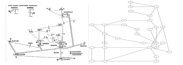
Figure 1: Left : Electrical representation of the IEEE network case 30. Right : schematic of the IEEE network case 30, from [14] using the Graphviz software [15].

For each index $i$, we compute the inverse of the eigenvalue $1/\omega_{i}^{2}$; it decays as a function of $i$ as shown in the left panel of Fig. 2. The norm of $\parallel\nabla\mathbf{v}^{i}\parallel_{\infty}$ increases with $i$ and has some maxima. It is shown in the right panel of Fig. 2. Note the peak for $i=19$ which corresponds to the eigenvector $\mathbf{v}^{19}$ such that $\mathbf{v}^{19}_{29}=+1/\sqrt{2},~{}~{}\mathbf{v}^{19}_{30}=-1/\sqrt{2},~{}~{}\mathbf{v}^{19}_{i}=0$ for $i$ different from $29,30$. The strict nodal domains are very small, $\{29\}\cup\{30\}$. This very special eigenvector was analyzed in our previous work [7], we termed it a closed swivel because only two nodes are non zero. On almost all nodes, no action is effective on the system on that particular eigenmode. The eigenvalue is $\omega^{2}_{19}=3$.

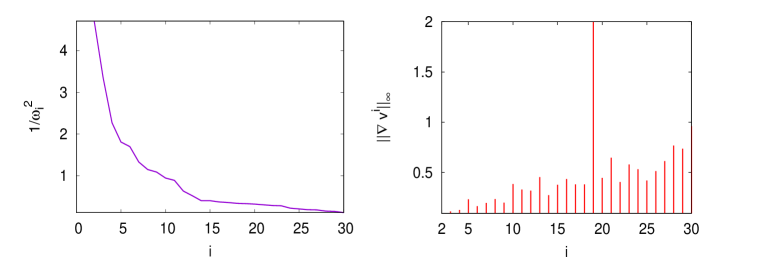
Figure 2: Plot as a function of $i$ of the inverse of the eigenvalue $1/\omega_{i}^{2}$ (left panel) and of $\parallel\nabla\mathbf{v}^{i}\parallel_{\infty}$ (right panel) .

The associated line power infinite norm $\parallel P_{l}\parallel_{\infty}$ which is the multiplication of the two different expressions is shown in Fig. 3.

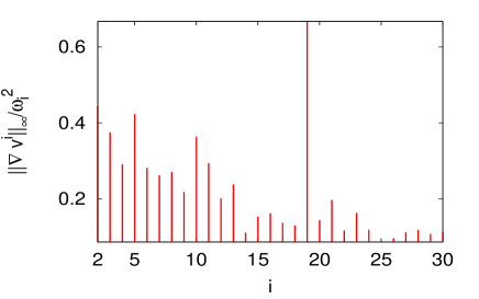
Figure 3: Plot of the line power infinite norm $\parallel P_{l}\parallel_{\infty}$ when $P=\mathbf{v}^{i}$ as a function of $i$.

This quantity is maximum for $i=19$, corresponding exactly to the swivel eigenvector discussed above. This eigenvector corresponds to the power being focused in the line between the two nodes of the swivel, giving the maximum $\parallel P_{l}\parallel_{\infty}$.

The other eigenvectors that give peaks in $\parallel P_{l}\parallel_{\infty}$ are $\mathbf{v}^{5}$ and $\mathbf{v}^{10}$. Their nodal domains are more complex than the one of $\mathbf{v}^{19}$ and are shown in Figs. 4 and 5. They both show strong gradients between nodal domains which explain the peaks in $\parallel P_{l}\parallel$. From Fig. 2 we expect that the vector $\mathbf{v}^{15}$ will contribute to $\parallel P_{l}\parallel_{\infty}$, however $\omega_{5}^{2}$ is large so that finally the contribution of $\mathbf{v}^{5}$ to $\parallel P_{l}\parallel_{\infty}$ is small.

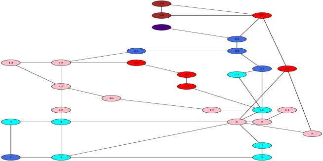
Figure 4: Nodal domains of the eigenvector $\mathbf{v}^{5}$. The color scheme for the components $\mathbf{v}^{5}_{i}$ is brown if $-0.3<\mathbf{v}^{5}_{i}$, red if $-0.3<\mathbf{v}^{5}_{i}<-0.1$, pink if $-0.1<\mathbf{v}^{5}_{i}<0$, cyan if $0<\mathbf{v}^{5}_{i}<0.1$ , royalblue if $0.1<\mathbf{v}^{5}_{i}<0.3$ and indigo if $0.3<\mathbf{v}^{5}_{i}$ .

The positive nodal domains are $A=\{10,21,22,23,24,25,26\}$ $B=\{1,2,3,4,5,7\}$. The negative nodal domains are $C=\{6,8,9,11,28,27,29,30\}$ and
$D=\{13,12,14,15,16,17,18,19,20\}$. Note the strong gradients at the interface between the positive and negative nodal domains. In particular between the nodes 27 and 25 because $-0.3<\mathbf{v}^{5}_{27}<-0.1$ and $0.1<\mathbf{v}^{5}_{25}<0.3$. This gradient is responsible for the peak observed for $i=5$ in Fig. 3. Notice also the strong gradient between nodes 15 and 23.

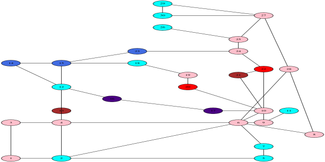
Figure 5: Nodal domains of the eigenvector $\mathbf{v}^{10}$, the color scheme is the same as for Fig. 4 .

The negative nodal domains are $A=\{1,3,4,13,6,8,9,10,19,20,21,22,24,25,27,28\}$. The positive nodal domains are $B=\{2,5,7\}$, $C=\{11\}$, $D=\{12,14,15,16,17,18,23\}$, $E=\{26\}$ and $F=\{29,30\}$. Notice the strong gradients between nodes 10 and 17 and 10 and 21. This explains the large amplitude in $\parallel\nabla\mathbf{v}^{i}\parallel_{\infty}$.

Figure 6: Schematic nodal domains of the eigenvectors $\mathbf{v}^{5}$ (left) and $\mathbf{v}^{10}$ (right).

The comparison between $\mathbf{v}^{5}$ and $\mathbf{v}^{10}$ is instructive. Fig. 6 shows the nodal domains for $\mathbf{v}^{5}$ (left) and $\mathbf{v}^{10}$ (right). There are four nodal domains for the former forming a cycle and six for the latter forming a star. There is no general theory predicting the shape and size of these domains, only an upper bound on their number depending on the order of the eigenvalue.

4.2 IEEE Case 118

The next example is the larger case118 with $n=118$ nodes, $m=186$ edges and an average degree $\bar{d}=2m/n=3.1$. Note that for this network, five lines have been doubled so that the Laplacian now has weights. The evolutions of $1/\omega_{i}^{2}$ and $\parallel\nabla\mathbf{v}^{i}\parallel_{\inf}$ are shown in Figs. 7 and 8. They are very similar to the ones for the case30. In particular, the inverse of the eigenvalues decay exponentially as shown in the lin-log scale of the left panel of Fig. 7.

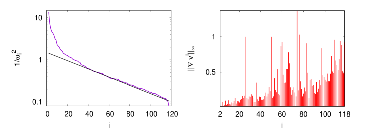
Figure 7: Plot as a function of $i$ of the inverse of the eigenvalue $1/\omega_{i}^{2}$ (left panel) and of $\parallel\nabla\mathbf{v}^{i}\parallel_{\infty}$ (right panel) .

Notice in the right panel of Fig. 7 the strong contributions to $\parallel\nabla\mathbf{v}^{i}\parallel_{\infty}$ of the eigenvectors $\mathbf{v}^{26},\mathbf{v}^{50},\mathbf{v}^{59},\mathbf{v}^{60},\mathbf{v}^{74},\mathbf{v}^{76}$ and $\mathbf{v}^{83}$. An extreme case is the swivel eigenvector [7] $\mathbf{v}^{26}$ such that $\mathbf{v}^{26}_{111}=+1/\sqrt{2},~{}~{}\mathbf{v}^{26}_{112}=-1/\sqrt{2},~{}~{}\mathbf{v}^{26}_{i}=0$ for $i$ different from $111,~{}112$. The eigenvalue is $\omega^{2}_{26}=1$. The eigenvector $\mathbf{v}^{50}$ is also a swivel. The other eigenvectors are localized in specific regions of the network. By this we mean that the eigenvector has a small number of components of absolute value much larger than the rest. For example $\mathbf{v}^{59}$ is localized from nodes 84 to 88. $\mathbf{v}^{60},\mathbf{v}^{83}$ from 100 to 118, $\mathbf{v}^{74}$ around 90 and $\mathbf{v}^{76}$ around 110. This localization comes as a surprise because the general theory of nodal domains does not predict it.

The associated line power infinite norm $\parallel P_{l}\parallel_{\infty}$ is shown in Fig. 8. Not all the peaks present in the right panel of Fig. 7 are present here. This is because of the increase of the eigenvalues $\omega^{2}_{i}$ with $i$. For example the large peaks $\mathbf{v}^{74},\mathbf{v}^{76}$ are now much smaller in Fig. 8. The swivel eigenvector $\mathbf{v}^{26}$ gives the largest contribution.

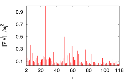
Figure 8: Plot of the line power infinite norm $\parallel P_{l}\parallel_{\infty}$ when $P=\mathbf{v}^{i}$ as a function of $i$.

To conclude this section, we have seen that $\nabla\mathbf{v}^{i}$ is related to nodal domains. We see a general trend showing that a linear interpolation of $\parallel\nabla\mathbf{v}^{i}\parallel$ shows a slow increase with $i$. However there are some peaks that correspond to highly localized eigenvectors. These highly localized eigenvectors $\mathbf{v}^{i}$ give a large contribution to $\nabla\mathbf{v}^{i}$. Some are due to geometrical configurations of the network like swivels. It is not clear where the others arise from.

In the next section, we consider general $P$ distributions. We will see that localized eigenvectors play an important role in $P_{l}$ for small $i$. When $i$ is large, their influence is mitigated by the denominator $\omega_{i}^{2}$.

5 Spectral solutions of the reduced load-flow

In this section, we combine the graph information with the generator / load vector and calculate the power in the lines $P_{l}$.

5.1 A small size network : effect of soft nodes

Before addressing networks with a relatively large number of nodes it is useful to consider a very simple example where calculations can be conducted by hand. This shows the usefulness of the approach.

We consider the simple 6 node network shown in Fig. 9.

Figure 9: A 6-node electrical network.

The graph Laplacian here is

$$\Delta=\begin{pmatrix}5&-1&-1&-1&-1&-1\cr-1&2&-1&0&0&0\cr-1&-1&2&0&0&0\cr-1&0&0&3&-1&-1\cr-1&0&0&-1&2&0\cr-1&0&0&-1&0&2\end{pmatrix},$$ (24)

whose eigenvalues $\omega_{i}^{2},~{}i=1,\dots,6$ are

$$0,~{}~{}~{}1,~{}~{}~{}2,~{}~{}~{}3,~{}~{}~{}4,~{}~{}~{}6$$ (25)

corresponding to the eigenvectors

$$\mathbf{v}^{1}={1\over{\sqrt{6}}}(1,1,1,1,1,1)^{T},~{}~{}~{}~{}\mathbf{v}^{2}={1\over\sqrt{30}}(0,3,3,-2,-2,-2)^{T},$$

$$\mathbf{v}^{3}={1\over\sqrt{2}}(0,0,0,0,1,-1)^{T},~{}~{}~{}~{}\mathbf{v}^{4}={1\over{\sqrt{2}}}(0,1,-1,0,0,0)^{T},$$

$$\mathbf{v}^{5}={1\over\sqrt{6}}(0,0,0,2,-1,-1)^{T},~{}~{}~{}~{}\mathbf{v}^{6}={1\over\sqrt{30}}(-5,1,1,1,1,1)^{T},.$$

The associated gradients are

$\nabla\mathbf{v}^{2}$	$(-0.55,0,0.55,0.36,0,-0.36,0.36,0)^{T}$
$\nabla\mathbf{v}^{3}$	$(0,0,0,0,-0.71,0.71,0.71,0.71)^{T}$,
$\nabla\mathbf{v}^{4}$	$(0.71,-1.41,0.71,0,0,0,0,0)^{T}$,
$\nabla\mathbf{v}^{5}$	$(0,0,0,0.82,-1.22,0.41,-0.41,-1.22)^{T}$,
$\nabla\mathbf{v}^{6}$	$(-1.09,0,1.09,-1.09,0,1.09,-1.09,0)^{T}$

The power in the lines is then

$$P_{l}=p_{2}{\nabla\mathbf{v}^{2}\over 1}+p_{3}{\nabla\mathbf{v}^{3}\over 2}+p_{4}{\nabla\mathbf{v}^{4}\over 3}+p_{5}{\nabla\mathbf{v}^{5}\over 4}+p_{6}{\nabla\mathbf{v}^{6}\over 6},$$ (26)

where $p_{i}$ is the projection of $P$ on the eigenvector $\mathbf{v}^{i}$, see (16). Expression (26) suggests that a large $p_{2}$ will contribute significantly more to $P_{l}$ than a large $p_{5}$ or $p_{6}$.

When the eigenvector $\mathbf{v}^{i}$ has a zero component at node $k$, $\mathbf{v}^{i}_{k}=0$ ( a soft node in the language of [7]), the $p_{i}$ coefficient does not depend on what is at node $k$. This is because $p_{i}=P\cdot\mathbf{v}^{i}$. In particular, if there is a generator at node $k$, it will not contribute to $p_{i}$. This reduces the number of directions for minimizing $\parallel P_{l}\parallel$.

To see these effects in more detail, we first assume that the loads are equally distributed over the network and study how placing a single generator on the network affects $P_{l}$. To examine the contribution of the different modes $\mathbf{v}^{i}$ to $P_{l}$, we introduce the partial sums

$$s_{k}^{\infty}=\parallel\sum_{i=2}^{k}(g_{i}-l_{i}){\nabla\mathbf{v}^{i}\over\omega_{i}^{2}}\parallel_{\infty},$$ (27)

$$s_{k}^{2}=\sum_{i=2}^{k}{(g_{i}-l_{i})^{2}\over\omega_{i}^{2}}.$$ (28)

Note that $s_{n}^{2}=\parallel P_{l}\parallel^{2}_{2}$ and $s_{n}^{\infty}=\parallel P_{l}\parallel_{\infty}$.

position
of generator	1	2	4	6
$p_{2}$	0	-3.29	2.19	2.19
$p_{3}$	0	0	0	-4.24
$p_{4}$	0	4.24	0	0
$p_{5}$	0	0	5	-2.44
$p_{6}$	5.48	-1.09	-1.09	-1.09
$\parallel P_{l}\parallel_{\infty}$	1	3	2	2.75
$\parallel P_{l}\parallel_{2}$	2.24	4.12	3.32	3.94

Table 1: Power coefficients $p_{i}$, $\parallel P_{l}\parallel_{\infty}$, $\parallel P_{l}\parallel_{2}$ for different generator positions. The loads are uniformly distributed.

Table 1 shows the coefficients $p_{i}$ for a generator of strength 6 placed at nodes 1, 2 or 4. A generator at node 1 will be such that only $p_{6}$ is non zero. Then we expect that $\parallel P_{l}\parallel$ will be minimal and this is indeed the case. On the other hand, a generator placed at node 2 gives a large $p_{2}$ so that $\parallel P_{l}\parallel$ will be larger. As expected, we see in table 1 a correlation between large values of $p_{2}$ and $p_{3}$ and large values of $\parallel P_{l}\parallel$.

In a second set of experiments, we place two generators on the grid and examine how $P_{l}$ depends on their position. For this, we choose the following vector of loads

$$L=(1,2,1,3,0,1)^{T}.$$

First we assume that the generators are placed at nodes 1 and 2, so that $G=(G_{1},G_{2},0,0,0,0)^{T}$, where $G_{1}+G_{2}=\sum_{i}L_{i}$. Then the power vector is $P=(g-1,6-g,-1,-3,0,-1)^{T}$ where we replaced $G_{1}$ by $g$ to simplify the notation. In the following, Projecting $P$ onto the eigenvectors, we note that, because of the zero components $\mathbf{v}^{3}_{1}$ and $\mathbf{v}^{5}_{1}$, there are no $g$ dependent components on the eigenvectors $\mathbf{v}^{3}$ and $\mathbf{v}^{5}$; we find $\parallel P_{l}\parallel_{2}=2.7$. When the generators are now placed at nodes 1 and 5, $g$ terms will affect the components of $\mathbf{v}^{2},\mathbf{v}^{3},\mathbf{v}^{5}$ and $\mathbf{v}^{6}$. We then expect to find a higher maximum for $\parallel P_{l}\parallel_{2}$ and this is the case, $\parallel P_{l}\parallel_{2}=3.2$. Fig. 10 shows $\parallel P_{l}\parallel_{2}$ (blue online) and $\parallel P_{l}\parallel_{\infty}$ (red online) as a function of $g$ for the two different configurations. We see that $\parallel P_{l}\parallel_{2}$ for the 1-2 configuration (left) is always above $\parallel P_{l}\parallel_{2}$ for the 1-5 configuration (right). On the other hand, the minimum of $\parallel P_{l}\parallel_{\infty}$ is the same for both configurations.

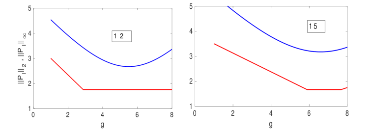
Figure 10: Plot of $\parallel P_{l}\parallel_{2}$ (blue online) and $\parallel P_{l}\parallel_{\infty}$ (red online) as a function of the strength $g$ of the generator at node 1, when the second generator is placed at node 2 (left panel) or at node 5 (right panel).

The flatness of $\parallel P_{l}\parallel_{\infty}$ for the 1-2 distribution (left of Fig. 10) is due to the zero first and second components for $\mathbf{v}^{i}$. On the other hand the 1-5 distribution has less zeros so the $\parallel P_{l}\parallel_{\infty}$ depends more on $g$. Fig. 10 also shows that for both configurations $1,2$ and $2,5$, we can simultaneously minimize the two norms.

We now place the 1st generator of amplitude $g$ at node 2 and the second one at nodes 4,5 and 6 respectively. Fig. 11 shows $\parallel P_{l}\parallel_{2}$ $\parallel P_{l}\parallel_{2}$ (blue online) and $\parallel P_{l}\parallel_{\infty}$ (red online) as a function of $g$.

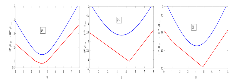
Figure 11: Plot of $\parallel P_{l}\parallel_{2}$ (blue online) and $\parallel P_{l}\parallel_{\infty}$ (red online) as a function of the strength $g$ of the generator at node 2, when the second generator is placed at nodes 4,5 and 6.

We see that the 2-4 configuration gives a minimum compared to the 2-5 and 2-6. This is clear because in this configuration, the $\mathbf{v}^{3}$ component of $P$ does not depend on $g$. Here, only the $2,4$ configuration (left of Fig. 11) leads to the same minimum for $\parallel P_{l}\parallel_{2}$ and $\parallel P_{l}\parallel_{\infty}$.

5.2 Convergence of $s_{k}^{2}$ with $k$: example of a grid

For the placement of two generators on a network, it is interesting to write $\parallel P_{l}\parallel_{2}^{2}$. Assuming the generators are positioned at nodes $p$ and $m$ , with amplitudes $G_{p}$ and $G_{m}$, we have

$$\parallel P_{l}\parallel_{2}^{2}=\sum_{i=2}^{n}{(g_{i}-l_{i})^{2}\over\omega_{i}^{2}}=\sum_{i=2}^{n}{(G_{p}v_{p}^{i}+G_{m}\mathbf{v}^{i}_{m}-l_{i})^{2}\over\omega_{i}^{2}}.$$

Expanding the squares and rearranging, we get the final expression

$$\parallel P_{l}\parallel_{2}^{2}=G_{p}^{2}\sum_{i}{(v_{p}^{i})^{2}\over\omega_{i}^{2}}+G_{m}^{2}\sum_{i}{(v_{m}^{i})^{2}\over\omega_{i}^{2}}$$

$$+\sum_{i}{l_{i}^{2}\over\omega_{i}^{2}}+2G_{p}G_{m}\sum_{i}{v_{p}^{i}v_{m}^{i}\over\omega_{i}^{2}}-2G_{p}\sum_{i}{v_{p}^{i}l_{i}\over\omega_{i}^{2}}-2G_{m}\sum_{i}{v_{m}^{i}l_{i}\over\omega_{i}^{2}}.$$ (29)

The coefficients of this polynomial in $G_{p},G_{m}$ are sums from $i=2$ to $n$. We have observed that they converge rapidly with $i$.

Simple systems on which to test this convergence are chains and grids (cartesian product of two chains). There, one can compute explicitly the eigenvectors and eigenvalues so that the network can be made arbitrarily large. A grid is also a first approximation of a transmission network.

A chain with $n$ nodes has eigenvalues $\omega^{2}_{i}$ and eigenvectors $\mathbf{v}^{i}$ whose components $\mathbf{v}^{i}_{p}$ are

$$\omega^{2}_{i}=4\sin^{2}{\pi(i-1)\over 2n},~{}~{}i=1,\dots,n$$ (30)

$$\mathbf{v}^{i}_{p}={1\over N_{i}}\cos[{\pi(i-1)\over n}(p-{1\over 2})],~{}~{}p=1,\dots,n$$ (31)

where the normalization factor is $N_{i}=\sqrt{n}$ if $i=1$ and $N_{i}=\sqrt{n/2}$ otherwise.

Let us consider $\parallel P_{l}\parallel^{2}_{2}$ for this network. From 20 we have

$$\parallel P_{l}\parallel^{2}_{2}=\sum_{i=2}^{n}{p_{i}^{2}\over\omega_{i}^{2}}={1\over 4}\sum_{i=2}^{n}{p_{i}^{2}\over\sin^{2}{\pi(i-1)\over 2n}}$$

The error committed when truncating the sum at $k\leq n$ is

$$\delta_{k}\equiv\parallel P_{l}\parallel^{2}_{2}-s_{k}^{2}={1\over 4}\sum_{i=k}^{n-1}{p_{i+1}^{2}\over\sin^{2}{\pi i\over 2n}}.$$

This quantity is positive and the sequence ${1\over\sin^{2}{\pi i\over 2n}}$ is decreasing so that $\delta_{k}$ has the following upper bound

$$\delta_{k}\leq{1\over 4}~{}~{}\underset{k+1\leq i\leq n}{\rm max}~{}(p_{i}^{2})~{}~{}\int_{k-1}^{n-1}{dx\over\sin^{2}{\pi x\over 2n}}.$$

Finally we obtain

$$\delta_{k}\leq{n\over 2\pi}~{}~{}\underset{k+1\leq i\leq n}{\rm max}~{}(p_{i}^{2})~{}~{}\left[\mathrm{cotan}{\pi(k-1)\over 2n}-\mathrm{cotan}{\pi(n-1)\over 2n}\right].$$ (32)

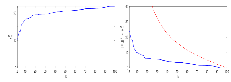
Figure 12: Plot of the partial sum $s_{k}^{2}$ (left) and the error $\delta_{k}$ (right) as a function of $k$ for a chain with $n=100$ nodes. The upper bound (32) is shown in dashed line (red online). See text for parameters.

To see how good the estimate (32) we studied a chain with $n=100$ nodes. The generator vector is such that $G(31)=1,~{}G(5)=3$, $0$ elsewhere and the load vector verifies $L(4)=2,~{}L(62)=1,~{}L(15)=1$ and $0$ elsewhere. The left panel of Fig. 12 shows the partial sum $s_{k}^{2}$ as a function of $k$. It reaches 80 % of its value for $k\approx n/5$. The error $\delta_{k}$ (right panel) decreases sharply for $k<n/5$, afterwards its decrease is much slower. The upper bound (32) is shown in dashed line (red online). The fairly large difference is due to $p_{i}^{2}$. This quantity depends on the eigenvectors and is difficult to estimate; the only option is to take the upper bound $\underset{k+1\leq i\leq n}{\rm max}p_{i}^{2}$. We will discuss this at the end of the section.

Consider now a grid formed by the cartesian product $C_{n}\times C_{m}$ of two chains $C_{n}$ and $C_{m}$ with $n$ and $m$ nodes respectively. Its eigenvalues are $\omega^{2}_{i,j}=\omega^{2}_{i}+\omega^{2}_{j}$ where $\omega^{2}_{i}$ is an eigenvalue for $C_{n}$ while $\omega^{2}_{j}$ is an eigenvalue for $C_{m}$. The associated eigenvector is $\mathbf{v}^{ij}=\mathbf{v}^{i}\otimes\mathbf{v}^{j}$, the Kronecker product of $\mathbf{v}^{i}$ and $\mathbf{v}^{j}$ (more details can be found in the book [9]). The eigenvalue $\omega^{2}_{i,j}$ and the components $\mathbf{v}^{ij}_{pq}$ are

$$\omega^{2}_{i,j}=4\left[\sin^{2}{\pi(i-1)\over 2n}+\sin^{2}{\pi(j-1)\over 2m}\right],$$ (33)

$$\mathbf{v}^{ij}_{pq}=\mathbf{v}^{i}_{p}\mathbf{v}^{j}_{q}={1\over N_{p}N_{q}}\cos[{\pi(i-1)\over n}(p-{1\over 2})]\cos[{\pi(j-1)\over m}(q-{1\over 2})],$$ (34)

where $i,p\in\{1,\dots,n\},~{}~{}~{}j,q\in\{1,\dots,m\}$ and where the normalization factors $N_{p},N_{q}$ follow the rules of the chains.

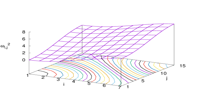
Figure 13: Eigenvalues $\omega^{2}_{i,j}$ as a function of $i,j$ for a grid $n=7,m=15$. On the bottom we show the level sets ranging from $0$ to $8$ and separated by $0.25$.

The eigenvalues $\omega^{2}_{i,j}$ are such that $\omega^{2}_{i,j}\leq 8$. They increase monotonically with $i$ and $j$ as shown in Fig. 13; there the contour lines are separated by $0.25$.

The expression of $\parallel P_{l}\parallel_{2}^{2}$ is

$$\parallel P_{l}\parallel_{2}^{2}=\sum_{i}^{n}\sum_{j}^{n}{p_{ij}^{2}\over\omega^{2}_{ij}},$$ (35)

where $p_{ij}$ is the component of the power on the eigenvector $\mathbf{v}^{ij}$ and where $p_{11}=0$. The sum is written so for ease of notation, the term $i=j=1$ should be omitted because $\omega_{11}=0$. Let us consider the residual

$$\delta_{k,l}\equiv\parallel P_{l}\parallel_{2}^{2}-\sum_{i}^{k}\sum_{j}^{l}{p_{ij}^{2}\over\omega^{2}_{ij}}.$$ (36)

Assume for simplicity $n=m,~{}~{}k=l$. We have

$$\delta_{k,k}\leq{1\over 4}~{}~{}\underset{k+1\leq i,j\leq n}{\rm max}(p_{ij}^{2})~{}~{}\sum_{i,j=k}^{n}{1\over\sin^{2}{\pi i\over 2n}+\sin^{2}{\pi j\over 2n}}\leq{1\over 4}~{}~{}\underset{k+1\leq i,j\leq n}{\rm max}(p_{ij}^{2})~{}~{}I_{2}(k),$$

where $I_{2}$ is the integral over the strip $S$, see Fig. 14

$$I_{2}(k)=\iint_{S}{dxdy\over\sin^{2}{\pi x\over 2n}+\sin^{2}{\pi y\over 2n}}$$ (37)

Figure 14: Integration domain for $I_{2}$ in the $(x,y)$ plane.

The integrand in $I_{2}$ is positive so $I_{2}$ can be bounded from above by the integral on the quarter annulus $A$ bounded by the circles $C_{1}$ and $C_{2}$ shown in Fig. 14. We have

$$I_{2}=({2n\over\pi})^{2}\iint_{{\pi(k-1)\over 2n}\leq w,z\leq{\pi(n-1)\over 2n}}{dwdz\over\sin^{2}w+\sin^{2}z}.$$

The function $\sin^{2}(r\cos\theta)+\sin^{2}(r\sin\theta)$ is minimum for $\theta=\pi/4$ so that

$${1\over\sin^{2}(r\cos\theta)+\sin^{2}(r\sin\theta)}\leq{1\over 2\sin^{2}(r/\sqrt{2})}.$$

Then

$$\delta_{k,k}\leq~{}~{}({n\over\pi})^{2}\underset{k+1\leq i,j\leq n}{\rm max}(p_{ij}^{2})~{}~{}\int_{0}^{\pi/2}d\theta\int_{\pi(k-1)\over 2n}^{\pi(n-1)\over n\sqrt{2}}{rdr\over\sin^{2}{\pi r\over\sqrt{2}}},$$

and further calculations yield the final result

$$\delta_{k,k}\leq n^{2}\underset{k+1\leq i,j\leq n}{\rm max}(p_{ij}^{2})~{}~{}\left[\mathrm{cotan}{\pi(k-1)\over 2\sqrt{2}n}-\mathrm{cotan}{\pi(n-1)\over 2n}\right].$$ (38)

The dominant term is the first $\mathrm{cotan}$. It is large for $k$ small and decays quickly as $k$ increases. For ${k-1\over 2\sqrt{2}n}=0.2$ $\mathrm{cotan}{\pi(k-1)\over 2\sqrt{2}n}\approx 1.37$. Again, this upper bound is not sharp because of the crude bound on $p_{ij}^{2}$.

To analyze the effects of $p_{ij}^{2}$, we have to fix the distribution of generators and loads. Assume as in the beginning of the section that we only have two generators placed at nodes $p$ and $m$ and uniform loads. Then, we can use expression (29) for $\parallel P_{l}\parallel_{2}^{2}$. For the grid, the indices $i,m$ are associated to four indices $(p,q),~{}~{}(r,s)$. This means that we place one generator at position $(p,q)$ and another at $(r,s)$. Assume these positions are fixed; we introduce the partial sum

$$s_{k}^{2}=\sum_{i,j=1}^{k}{\mathbf{v}^{ij}_{pq}\mathbf{v}^{ij}_{rs}\over\omega^{2}_{i,j}},$$ (39)

with the restriction that we omit the term $i=j=1$. To examine how $s_{k}^{2}\to s_{n}^{2}$, we considered a grid of size $n=61,m=61$ and computed $s_{k}^{2}$ for $(p,q,r,s)=(10,4,20,28),(10,4,10,28),(4,4,6,6)$ and $(4,4,15,15)$. The results are shown in Fig. 15.

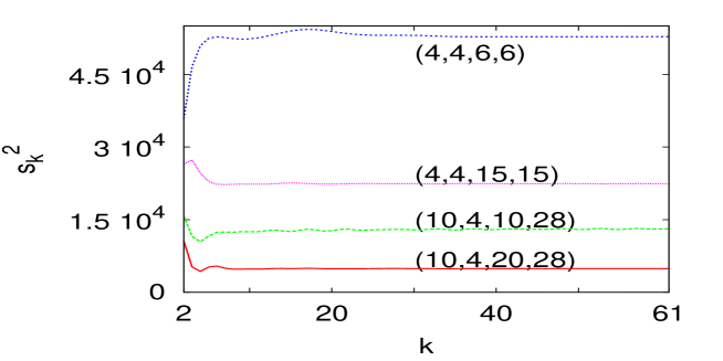
Figure 15: Partial sums $s_{k}^{2}=\sum_{ij}^{k}{\mathbf{v}^{ij}_{pq}\mathbf{v}^{ij}_{rs}\over\omega^{2}_{i,j}},$ as function of $k$ for different $(p,q,r,s)$ configurations.

In all cases, except for the close nodes configuration $(4,4,6,6)$, the sum converges for $k\approx 10$. For the $(4,4,6,6)$ the sum has converged for $k\approx 20\ll n$. We observe similar fast convergence of the other sums in expression (29).

5.3 The IEEE 30 network

There are only six generators in this network,

$$G_{1}=23.54,~{}G_{2}=60.97,~{}G_{13}=37,~{}G_{22}=21.59,~{}G_{23}=19.2,~{}G_{27}=26.91.$$ (40)

The loads are distributed uniformly over the network.

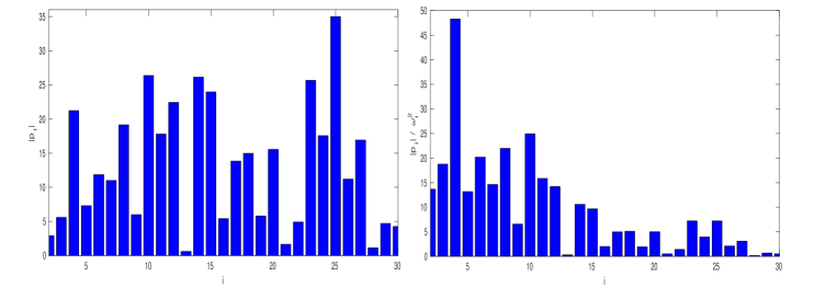
Figure 16: Plot of $|p_{i}|$ (left) and ${|p_{i}|\over\omega_{i}^{2}}$ (right) as a function of $i$ for the power vector $P$ of IEEE case 30.

The components of the power vector $P$ are shown in Fig. 16. As shown in the right panel, The right panel shows that, as expected, ${|p_{i}|\over\omega_{i}^{2}}$ decays with $i$.

First, we examine the convergence of $s_{k}^{\infty},~{}~{}s_{k}^{2}$ as $k$ increases. The graph is shown in Fig. 17.

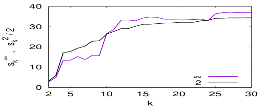
Figure 17: Plot of the partial sums $s_{k}^{\infty}$, $s_{k}^{2}/2$ from (27,28) as a function of ${k}$.

Note how $s_{k}^{\infty}$ and $s_{k}^{2}$ increase fast up to ${k}=15$ terms. After that the rate of increase is much smaller. As expected, the small eigenvalues dominate the sum. Past $k=12$, the $L_{\infty}$ norm is stable while the $L_{2}$ norm continues to increase but at much slower rate.

We did not carry out a full optimization of the amplitudes of the generators since this is out of the scope of the article. Instead we varied the amplitudes $G_{i}$ for to examine how the power in the lines varies. We show two cases in the table below

	$G_{1}$	$G_{2}$	$G_{13}$	$G_{22}$	$G_{23}$	$G_{27}$	$\parallel P_{l}\parallel_{2}$	$\parallel P_{l}\parallel_{\infty}$
original	23.54	60.97	37	21.59	19.2	26.91	68.78	37.
case 2	3.54	60.97	37	21.59	29.2	36.91	63.26	21.07

Table 2: Two different configurations of generators for IEEE case 30 with their associated line powers $\parallel P_{l}\parallel_{2}$ and $\parallel P_{l}\parallel_{\infty}$. The terms that have changed from the original configuration are written in bold.

We computed the partial sum $s_{k}^{\infty}$ as a function of ${k}$ for the four different configurations of table 2 in Fig. 18.

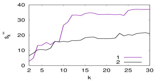
Figure 18: Plot of the partial sum (27) as a function of $n$ for the two configurations original (0) and case 2, shown in table 2.

The configuration 2 has a much lower value of $s_{k}^{\infty}$ than the other configuration. To show the importance of the modal distribution of power, we plot in Fig. 19 $|p_{i}|/\omega_{i}^{2}$ as a function of $i$ for the two configurations.

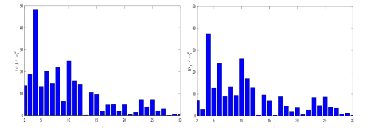
Figure 19: Plot of $|p_{i}|/\omega_{i}^{2}$ for the original configuration (left) and the improved configuration (right) shown in table 2.

Indeed, we see that configuration 2 has smaller $|p_{i}|$ for $i<15$ than the original configuration. This explains the difference in $\parallel P_{l}\parallel_{2}$ and especially $\parallel P_{l}\parallel_{\infty}$. This experiment shows that by tuning the amplitude of existing generators one can decrease significantly the power in the lines. We will carry out such an optimization in a further study.

5.4 The IEEE 118 network

The components of the power vector are shown in Fig. 20.

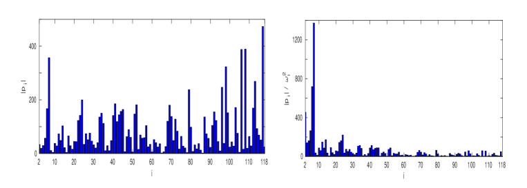
Figure 20: Plot of $|p_{i}|$ (left) and ${|p_{i}|\over\omega_{i}^{2}}$ (right) as a function of $i$ for the power vector $P$ of IEEE case 118.

A peak observed in $|p_{7}|$ in both panels. It corresponds to reinforcing the localized eigenvector $\mathbf{v}^{7}$. The large components of $p_{i}$ are smoothed out in the right panel by the denominator $\omega_{i}^{2}$.

We examine the convergence of $s_{k}^{\infty},~{}~{}s_{k}^{2}$ as ${k}$ increases. The graph is shown in Fig. 21.

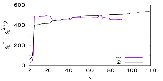
Figure 21: Plot of the partial sums $s_{k}^{\infty}$ $s_{k}^{2}/2$ from (27,28) as a function of ${k}$.

As for case 30, both $s_{k}^{\infty}$ and $s_{k}^{2}$ stabilize after 10 to 15 terms and again the small eigenvalues dominate the sum.

6 Conclusion and discussion

We have shown that the load-flow equations can be reduced to a singular linear system involving the graph Laplacian. Using the a basis of eigenvectors of the Laplacian, we introduced a spectral method to solve the load-flow equations. This provides a geometrical picture of the power flow on the network, very similar to a Fourier decomposition.

This spectral method provides an explicit expression of $P_{l}$ as a sum of components $\nabla\mathbf{v}^{i}/\omega_{i}^{2}$, where $\omega_{i}^{2},~{}~{}\mathbf{v}^{i}$ are respectively the $i$th eigenvalue and associated eigenvector of the Laplacian. These two components play different roles. The eigenvalues $\omega_{i}^{2}$ typically increase with $i$ so that the small $i$ ’s will generally control the sum. The term $\nabla\mathbf{v}^{i}$ is more difficult to estimate; it measures the space scale of the contribution on the network and is loosely related to the nodal domains of $\mathbf{v}^{i}$. Also, special eigenvectors $\mathbf{v}^{i}$ are strongly localized in a given region of the network and will dominate $P_{l}$ if $i$ is small. Soft nodes, where the eigenvector has zero components also turned out to be important for optimization.

Using the orthogonality of $\mathbf{v}^{i}$, we obtained a Parseval-like expression of $\parallel P_{l}\parallel_{2}$. Numerical studies show that the main contribution to $\parallel P_{l}\parallel_{2}$ and especially to $\parallel P_{l}\parallel_{\infty}$ tends to come from the small $i$ eigenvalues and eigenvectors, these correspond to large nodal domains i.e. large scales on the network. For example, only 10 or 20 modes are necessary to get a good estimate for a grid network of 30 nodes. For a 118 node network, 15 modes are sufficient to describe the solution with a 5 % accuracy. These numerical results are confirmed by analysis done on a chain and a grid.

This geometric approach could complement the standard nonlinear load-flow because it gives a global view of the network and the power vector. Because of this, in view of the growing portion of intermittent sources, our spectral approach could allow to optimize and reconfigure networks rapidly.

Acknowledgements

The authors are funded by Agence Nationale de la Recherche grant ”Fractal grid”. The calculations were done at the CRIANN computing center.

References

- [1] S. Backhaus and M. Chertkov, ”Getting a grip on the electrical grid”, Physics today 66 (5), 42 (2013).
- [2] P. Kundur, ”Power System Stability and Control” , Mac Graw-Hill, (1994).
- [3] J. Grainger, Jr. W. Stevenson and Gary W. Chang , ”Power Systems Analysis”, McGraw-Hill (2015).
- [4] D. Cvetkovic, P. Rowlinson and S. Simic, ”An Introduction to the Theory of Graph Spectra”, London Mathematical Society Student Texts (No. 75), (2001).
- [5] G. Dahlquist, A. Bjorck and N. Anderson, ”Numerical methods”, Prentice Hall, (1974).
- [6] D. K. Molzahn, C. Josz, I. A. Hiskens and P. Panciatici, arxiv.1507.07212
- [7] J.G. Caputo, A. Knippel and E. Simo, J. Phys. A: Math. Theor. 46, 035100, (2013).
- [8] W. H. Press , S. A. Teukolsky , W. T. Vetterling , B. P. Flannery , ”Numerical Recipes: The Art of Scientific Computing”, Cambridge University Press, (1986).
- [9] T. Biyikoglu, J. Leydold and P. Stadler, ”Laplacian eigenvectors of graphs”, Springer (2000).
- [10] E. B. Davies, G. M. L. Gladwell, J; Leydold and P. F. Stadler, ”Discrete nodal domain theorems”, Linear Algebra and its Applications 336 (2001) 51-60 .
- [11] M. Fiedler, Algebraic connectivity of graphs, Czechoslovak Math. J., 23(98) (1973), 298-305.
- [12] B. Mohar in ”The Laplacian spectrum of graphs, Graph Theory, Combinatorics and Applications”, Vol. 2, Ed. Y. Alavi, G. Chartrand, O. R. Oellermann, A. J. Schwenk, Wiley, pp. 871–898, (1991).
- [13] http://www.pserc.cornell.edu/matpower/
- [14] https://www2.ee.washington.edu/research/pstca/pf30/pg_tca30bus.htm
- [15] https://www.graphviz.org/