On Stronger Types of Locating-Dominating Codes

Abstract

Locating-dominating codes in a graph find their application in sensor networks and have been studied extensively over the years. A locating-dominating code can locate one object in a sensor network, but if there is more than one object, it may lead to false conclusions. In this paper, we consider stronger types of locating-dominating codes which can locate one object and detect if there are multiple objects. We study the properties of these codes and provide bounds on the smallest possible size of these codes, for example, with the aid of the Dilworth number and Sperner families. Moreover, these codes are studied in trees and Cartesian products of graphs. We also give the complete realization theorems for the coexistence of the smallest possible size of these codes and the optimal locating-dominating codes in a graph.

1 Introduction

Sensor networks are systems designed for environmental monitoring. Various location detection systems such as fire alarm and surveillance systems can be viewed as examples of sensor networks. For location detection, a sensor can be placed in any location of the network. The sensor monitors its neighbourhood (including the location of the sensor itself) and reports possible objects or irregularities such as a fire or an intruder in the neighbouring locations. In the model considered in the paper, it is assumed that a sensor can distinguish whether the irregularity is in the location of the sensor or in the neighbouring locations (as in  [21, 24, 25]). Based on the reports of the sensors, a central controller attempts to determine the location of a possible irregularity in the network. Usually, the aim is to minimize the number of sensors in the network. More explanation regarding location detection in sensor networks can be found in [9, 17, 22]. An online bibliography on the topic can be found at [18].

A sensor network can be modelled as a simple and undirected graph $G=(V(G),E(G))=(V,E)$ as follows: the set of vertices $V$ of the graph represents the locations of the network and the edge set $E$ of the graph represents the connections between the locations. In other words, a sensor can be placed in each vertex of the graph and the sensor placed in the vertex $u$ monitors $u$ itself and the vertices neighbouring $u$. Moreover, besides being simple and undirected we also assume that the graphs in this paper are finite. In what follows, we present some basic terminology and notation regarding graphs. The open neighbourhood of $u\in V$ consists of the vertices adjacent to $u$ and it is denoted by $N(u)$. The closed neighbourhood of $u$ is defined as $N[u]=\{u\}\cup N(u)$. The degree of a vertex $u$ is the number of vertices in the open neighbourhood $N(u)$ and the maximum degree $\Delta(G)=\Delta$ of the graph $G$ is the maximum degree among all the vertices of $G$. The distance between two vertices $d(u,v)$ is the number of edges in any shortest path connecting them. A non-empty subset $C$ of $V$ is called a code and the elements of the code are called codewords. In this paper, the code $C$ (usually) represents the set of locations where the sensors have been placed on. For the set of sensors monitoring a vertex $u\in V$, we use the following notation:

$$I(u)=N[u]\cap C\text{.}$$

In order to emphasize the graph $G$ and/or the code $C$, we sometimes write $I(u)=I(C;u)=I(G,C;u)$. We call $I(u)$ the $I$-set or the identifying set of $u$.

As stated above, a sensor $u\in V$ reports that an irregularity has been detected if there is (at least) one in the closed neighbourhood $N[u]$. In the model of the paper, we further assume that a sensor $u\in V$ reports $2$ if there is an irregularity in $u$, it reports $1$ if there is one in $N(u)$ (and none in $u$ itself), and otherwise it reports $0$. In other words, a sensor can distinguish whether an irregularity is in the location of the sensor or in the neighbouring locations. We say that a set (or a code) $C$ is dominating in $G$ if $I(C;u)$ is non-empty for all $u\in V\setminus C$. In other words, an irregularity in the network can be detected (albeit not located). Furthermore, the smallest cardinality of a dominating set in $G$ is called the domination number and it is denoted by $\gamma(G)$. Notice then that if the sensors in the code $C$ are located in such places that $I(C;u)$ is non-empty and unique for all $u\in V\setminus C$, then an irregularity in the network can be located by comparing $I(C;u)$ to $I$-sets of other non-codewords. This leads to the following definition of locating-dominating codes (or sets), which were first introduced by Slater in [21, 24, 25].

Definition 1.

A code $C\subseteq V$ is locating-dominating in $G$ if for all distinct $u,v\in V\setminus C$ we have $I(C;u)\neq\emptyset$ and

$$I(C;u)\neq I(C;v)\text{.}$$

A locating-dominating code $C$ in a finite graph $G$ with the smallest cardinality is called optimal and the number of codewords in an optimal locating-dominating code is denoted by $\gamma^{LD}(G)$. The value $\gamma^{LD}(G)$ is also called the location-domination number.

The previous definition of locating-dominating codes is illustrated in the following example.

Example 2.

Let $G$ be the graph illustrated in Figure 1. Consider the code $C=\{b,d,f\}$ in $G$ (see Figure 1). Since the $I$-sets $I(C;a)=\{b,d\}$, $I(C;c)=\{b,f\}$ and $I(C;e)=\{b,d,f\}$ are all non-empty and different, the code $C$ is locating-dominating in $G$. Moreover, there do not exist smaller locating-dominating codes in $G$ as using at most two codewords we can form at most three different non-empty $I$-sets. Therefore, we have $\gamma^{LD}(G)=3$.

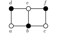
Figure 1: Optimal locating-dominating code in a graph $G$

The original concept of locating-dominating codes has some issues in certain types of applications. Firstly, locating-dominating codes might output misleading results if there exist more than one irregularity in the graph. For instance, if in the previous example there exist irregularities in $a$ and $c$, then the sensors located at $b$, $d$ and $f$ are reporting $1$. Now the system deduces that the irregularity is in $e$. Hence, a completely false output is given and we do not even notice that something is wrong. Secondly, in order to determine the location of the irregularity, we have to compare the obtained $I$-set to other such sets. In order to overcome these issues, so called self-locating-dominating and solid-locating-dominating codes have been introduced in [16] motivated by $(1,\leq 1)^{+}$-identifying or self-identifying codes introduced in [12, 14, 15]. For more detailed discussion on the motivation of self-locating-dominating and solid-locating-dominating codes, the interested reader is referred to [16]. The formal definitions of these codes are given in the following.

Definition 3.

A code $C\subseteq V$ is self-locating-dominating in $G$ if, for all $u\in V\setminus C$, we have $I(C;u)\neq\emptyset$ and

$$\bigcap_{c\in I(C;u)}N[c]=\{u\}\text{.}$$

A self-locating-dominating code $C$ in a finite graph $G$ with the smallest cardinality is called optimal and the number of codewords in an optimal self-locating-dominating code is denoted by $\gamma^{SLD}(G)$. The value $\gamma^{SLD}(G)$ is also called the self-location-domination number.

Definition 4.

A code $C\subseteq V$ is solid-locating-dominating in $G$ if $I(C;u)\neq\emptyset$ for every $u\in V\setminus C$ and, for all distinct $u,v\in V\setminus C$, we have

$$I(C;u)\setminus I(C;v)\neq\emptyset\text{.}$$

Note that this condition is equivalent with $I(C;u)\not\subseteq I(C;v)$. A solid-locating-dominating code $C$ in a finite graph $G$ with the smallest cardinality is called optimal and the number of codewords in an optimal solid-locating-dominating code is denoted by $\gamma^{DLD}(G)$. The value $\gamma^{DLD}(G)$ is also called the solid-location-domination number.

By the previous definitions, it is immediate that any self-locating-dominating and solid-locating-dominating code is also locating-dominating (see also Corollary 7) and that every graph contains a self-locating-dominating and solid-locating-dominating code. Indeed, $C=V$ is always a self-locating-dominating and solid-locating-dominating code. The definitions are illustrated in the following example. In particular, we show that the given definitions are indeed different.

Example 5.

Let $G$ be a graph illustrated in Figure 2. Let $C$ be a self-locating-dominating code in $G$. Observe first that if $a\notin C$, then $I(C;a)\subseteq\{b,d\}$ and we have

$$\{a,e\}\subseteq\bigcap_{x\in I(C;a)}N[x]\text{.}$$

This implies a contradiction and, therefore, the vertex $a$ belongs to $C$. An analogous argument also holds for the vertices $c$, $d$ and $f$. Hence, we have $\{a,c,d,f\}\subseteq C$. Moreover, the code $C_{1}=\{a,c,d,f\}$, which is illustrated in Figure 2(a), is self-locating-dominating in $G$ since for the non-codewords $b$ and $e$ we have $I(C_{1};b)=\{a,c\}$ and $N[a]\cap N[c]=\{b\}$, and $I(C_{1};e)=\{d,f\}$ and $N[d]\cap N[f]=\{e\}$. Hence, $C_{1}$ is an optimal self-locating-dominating code in $G$ and we have $\gamma^{SLD}(G)=4$.

Let us then consider the code $C_{2}=\{a,b,c\}$, which is illustrated in Figure 2(b). Now we have $I(C_{2};d)=\{a\}$, $I(C_{2};e)=\{b\}$ and $I(C_{2};f)=\{c\}$. Therefore, it is easy to see that $C_{2}$ is a solid-locating-dominating code in $G$. Moreover, there are no solid-locating-dominating codes in $G$ with smaller number of codewords since even a regular locating-dominating code has always at least $3$ codewords by Example 2. Thus, $C_{2}$ is an optimal solid-locating-dominating code in $G$ and we have $\gamma^{DLD}(G)=3$.

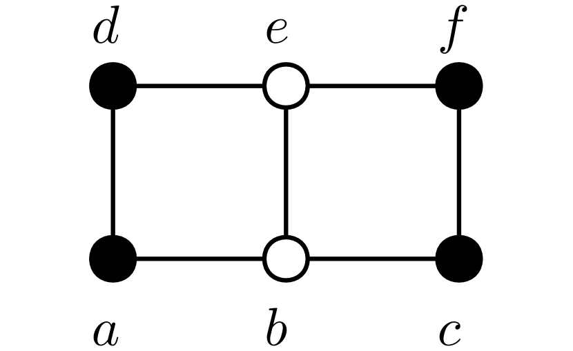
(a) Self-locating-dominating
     code

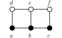
(b) Solid-locating-dominating
     code

Figure 2: Optimal self-locating-dominating and solid-locating-dominating codes in a graph $G$

In the previous example, we showed that the definitions of self-locating-dominating and solid-locating-dominating codes are different. Furthermore, by comparing Examples 2 and 5, we notice that the new codes are also different from the original locating-dominating codes. In the following theorem, we present new characterizations for self-locating-dominating and solid-locating-dominating codes. Comparing these characterizations to the original definitions of the codes, the differences of the codes become apparent. We omit the proof of the following theorem, because it is proved in [16] for connected graphs and it is easily modified for non-connected ones.

Theorem 6.

Let $G$ be a graph on at least two vertices.

• A code $C\subseteq V$ is self-locating-dominating if and only if, for all distinct $u\in V\setminus C$ and $v\in V$, we have $I(C;u)\setminus I(C;v)\neq\emptyset\text{.}$

• A code $C\subseteq V$ is solid-locating-dominating if and only if, for all $u\in V\setminus C$, we have $I(C;u)\neq\emptyset$ and

  $$\left(\bigcap_{c\in I(C;u)}N[c]\right)\setminus C=\{u\}\text{.}$$

By comparing Definition 4 and Theorem 6 (i) we notice that the only difference is that in $I(C;u)\setminus I(C;v)$ vertex $v$ can be a codeword when we consider self-location-domination. Similarly, when we compare Definition 3 and Theorem 6 (ii) we notice that the only difference is that in the case of solid-location-domination we omit codewords from the intersection.

The previous theorem together with the definition of solid-locating-dominating codes and the previous observation immediately gives the following corollary.

Corollary 7.

The following facts hold for all graphs $G$.

• If $C$ is a self-locating-dominating code in $G$, then $C$ is also solid-locating-dominating in $G$.

• If $C$ is a solid-locating-dominating code in $G$, then $C$ is also locating-dominating in $G$.

Thus, we have $\gamma^{LD}(G)\leq\gamma^{DLD}(G)\leq\gamma^{SLD}(G)$.

As stated earlier, self-locating-dominating and solid-locating-dominating codes have benefits over regular locating-dominating codes; they detect more than one irregularity and locate one irregularity without comparison to other $I$-sets — for more details, see [16].

Previously, when self-locating-dominating and solid-locating-dominating codes have been studied, in [16], the optimal values for $\gamma^{SLD}(K_{n}\square K_{m})$ and $\gamma^{DLD}(K_{n}\square K_{m})$ have been found. Also the a general lower bound for $\gamma^{SLD}(\mathbb{F}_{2}^{n})$ has been given and an infinite family of constructions attaining this bound is presented for suitable values of $n$. Moreover, a general lower bound for $\gamma^{DLD}(\mathbb{F}_{2}^{n})$ is given and this bound is shown to be asymptotically tight as $n$ grows.

In what follows, the structure of the paper is briefly discussed. In Section 2, we first show some general bounds and properties for self- and solid-locating-dominating codes; in particular, we utilize the Dilworth number and Sperner families. Then, in Section 3, we consider the codes in trees and determine self-location-domination and solid-location-domination numbers with the help of other graph parameters. In Section 4, we consider Cartesian products and give some general bounds for them which are shown to be achieved in the case of ladders and some rook’s graphs. Finally, in Section 5, we study the existence of graphs when we are given the location-domination number and the self-location-domination or the solid-location-domination number associated with them.

2 Basics

In this section, we present some basic results regarding self-locating-dominating and solid-locating-dominating codes. In particular, we give various lower and upper bounds for such codes. We first begin by giving results which do not take advantage of any properties or parameters of the graph such as the maximum degree or the independence number. Then, in Section 2.1, we use the Sperner’s Theorem to gain new bounds. Later, in Section 2.2, we apply the Dilworth number. Finally, in Section 2.3, we use independence number and consider complements of graphs.

In the following theorem, we begin by giving a simple upper bound for solid-locating-dominating codes in graphs. It is clear that the discrete graph $D_{n}$, with $n$ vertices and no edges, satisfies $\gamma^{DLD}(D_{n})=n$, because $V(D_{n})$ is its unique dominating set. We now focus on graphs with at least one edge.

Theorem 8.

If $G=(V,E)$ is a graph with order $n$ and size $m\geq 1$, then the code $V\setminus\{u\}$ is solid-locating-dominating in $G$ for any non-isolated vertex $u\in V$. Thus, we have

$$\gamma^{DLD}(G)\leq n-1.$$

Proof.

Let $u\in V$ be a non-isolated vertex of $G$, i.e., $N(u)\cap(V\setminus\{u\})\neq\emptyset$. By the definition, it is immediate that $V\setminus\{u\}$ is a solid-locating-dominating code of $G$. This further implies that $\gamma^{DLD}(G)\leq|V|-1$. ∎

The result of the previous theorem can also be interpreted as follows: in the particular case of graphs with no isolated vertices, none of the vertices of a graph is forced to be in all the solid-locating-dominating codes of the graph and hence, the same is also true for locating-dominating codes by Corollary 7. However, this is not the case with self-locating-dominating codes. Hence, for future considerations, we define the concept of forced codewords as follows: a vertex $u$ of $G$ is said to be a forced codeword regarding self-location-domination if $u$ belongs to all self-locating-dominating codes in $G$. In the following theorem, we give a simple characterization for forced codewords and show that such vertices indeed exist.

Theorem 9.

Let $G=(V,E)$ be a graph. If $|V|=1$, then the single vertex of the graph $G$ is a forced codeword. Assuming $|V|\geq 2$, a vertex $u\in V$ is a forced codeword regarding self-location-domination if and only if for some vertex $v\in V$ other than $u$ we have $N(u)\subseteq N[v]$.

Proof.

Let $C$ be a self-locating-dominating code in $G$ and $u$ be a vertex of $V$. If $|V|=1$, then due to the domination the single vertex is a forced codeword. Assume now that $|V|\geq 2$. Suppose further that there exists another vertex $v\in V$ such that $u\neq v$ and $N(u)\subseteq N[v]$. If $N(u)=\emptyset$, then again the domination yields that $u$ is a forced codeword. Suppose that $N(u)\neq\emptyset.$ This implies that if $u\notin C$, then

$$\{u,v\}\subseteq\bigcap_{c\in N(u)}N[c]\subseteq\bigcap_{c\in I(C;u)}N[c].$$

Therefore, as the previous intersection does not consist of a single vertex, the vertex $u$ belongs to $C$ and is a forced codeword.

Suppose then to the contrary that for any vertex $v\in V$ other than $u$ we have $N(u)\nsubseteq N[v]$, i.e., $N(u)\setminus N[v]\neq\emptyset$. Now choosing $C=V\setminus\{u\}(\neq\emptyset)$, we have $I(C;u)=N(u)$ and

$$\bigcap_{c\in I(C;u)}N[c]=\{u\}\text{.}$$

Therefore, by the definition, $C$ is a self-locating-dominating code in $G$. Thus, $u$ is not a forced codeword and we have a contradiction with the supposition. This concludes the proof of the theorem. ∎

By the previous theorem, we immediately observe that there exist graphs such that all the vertices are forced codewords. For example, the complete graphs and the complete bipartite graphs, where both independent sets of the partition have at least two vertices, are such extreme graphs.

2.1 Results based on Sperner’s Theorem

One of the fundamental results on locating-dominating codes by Slater [24] says that if $G$ is a graph with $n$ vertices and $\gamma^{LD}(G)=k$, then $n\leq k+2^{k}-1$. This result is based on the simple fact that using $k$ codewords at most $2^{k}-1$ distinct, non-empty $I$-sets can be formed. In what follows, we present an analogous result for self-locating-dominating and solid-locating-dominating codes. However, here it is not enough that all the $I$-sets are non-empty and unique, but we further require that none of the $I$-sets is included in another one. For this purpose, we present Sperner’s theorem, which considers the maximum number of subsets of a finite set such that none of the subsets is included in another subset. Sperner’s theorem has originally been presented in [26], and for more recent developments regarding the Sperner theory, we refer to [8].

Theorem 10 (Sperner’s theorem [26]).

Let $N$ be a set of $k$ elements and let $\mathcal{F}$ be a family of subsets of $N$ such that no member of $\mathcal{F}$ is included in another member of $\mathcal{F}$, i.e., for all distinct $X,Y\in\mathcal{F}$ we have $X\setminus Y\neq\emptyset$. Then we have

$$|\mathcal{F}|\leq\binom{k}{\left\lfloor\frac{k}{2}\right\rfloor}\text{.}$$

Moreover, the equality holds if and only if $\mathcal{F}=\{X\subseteq N\mid|X|=k/2\}$ when $n$ is even, and $\mathcal{F}=\{X\subseteq N\mid|X|=(k-1)/2\}$ or $\mathcal{F}=\{X\subseteq N\mid|X|=(k+1)/2\}$ when $n$ is odd.

A family of subsets satisfying the conditions of the previous theorem is called a Sperner family. In the following theorem, we apply Sperner’s theorem to obtain an upper bound on the order of a graph based on the number of codewords in a solid-locating-dominating (or self-locating-dominating) code.

Theorem 11.

Let $G$ be a graph with $n$ vertices and $C$ be a solid-locating-dominating code in $G$ with $k$ codewords. Then we have the following upper bound on the order of $G$:

$$n\leq k+\binom{k}{\left\lfloor\frac{k}{2}\right\rfloor}\text{.}$$

Proof.

Let $C$ be a solid-locating-dominating code in $G$ with $k$ codewords. By the definition, for any distinct $u,v\in V\setminus C$, we have $I(C;u)\setminus I(C;v)\neq\emptyset$. Therefore, the $I$-sets of non-codewords of $G$ form a Sperner family of subsets of $C$. Thus, by Sperner’s theorem, we obtain that

$$|V\setminus C|=n-k\leq\binom{k}{\left\lfloor\frac{k}{2}\right\rfloor}\text{.}$$

Hence, the claim immediately follows. ∎

Observe that the previous theorem also holds for self-locating-dominating codes due to Corollary 7. Furthermore, the upper bound of the theorem can be attained even for self-locating-dominating codes as is shown in the following example.

Example 12.

Let $k$ be a positive integer and $\ell$ be an integer such that $\ell=\binom{k}{\left\lfloor k/2\right\rfloor}$. Consider then a bipartite graph $G$ with the vertex set $U\cup V$, where $U=\{u_{1},u_{2},\ldots,u_{k}\}$ and $V=\{v_{1},v_{2},\ldots,v_{\ell}\}$. There are no edges within the sets $U$ and $V$, and the edges between the two sets are defined as follows. Let $\mathcal{F}$ be a (maximum) Sperner family of $U$ attaining the upper bound of Theorem 10 with each subset of $\mathcal{F}$ having $\lfloor k/2\rfloor$ elements. Recall that the number of subsets in $\mathcal{F}$ is $\ell$. Denoting the subsets of $\mathcal{F}$ by $F_{1},F_{2},\ldots,F_{\ell}$, we define the edges of each $v_{i}$ as follows: $v_{i}$ is adjacent to the vertices of $F_{i}$.

Now the code $C=U$ is self-locating-dominating in $G$. Indeed, the $I$-sets of the non-codewords in $V$ form a Sperner family and, hence, the characterization (i) of Theorem 6 is satisfied. Thus, $C$ is a self-locating-dominating code in $G$ with $k$ codewords and $G$ is a graph with $k+\binom{k}{\left\lfloor k/2\right\rfloor}$ vertices.

In the following immediate corollary of Theorem 11, we give a lower bound on the minimum size of solid-locating-dominating and self-locating-dominating codes based on the order of a graph. Notice also that the obtained lower bounds can be attained by the construction given in the previous example.

Corollary 13.

Let $G$ be a graph with $n$ vertices and let $k$ be the smallest integer such that $n\leq k+\binom{k}{\left\lfloor k/2\right\rfloor}$. Then we have

$$\gamma^{SLD}(G)\geq\gamma^{DLD}(G)\geq k\text{.}$$

2.2 Results using the Dilworth Number

In what follows, we are going to present some results on self-location-domination and solid-location-domination based on certain properties or parameters of graphs. For this purpose, we first present some definitions and notation. Let $u$ and $v$ be distinct vertices of $G$. We say that $u$ and $v$ are false twins if $N(u)=N(v)$ and that $u$ and $v$ are true twins if $N[u]=N[v]$. Furthermore, we say that $u$ and $v$ are twins if they are false or true twins. Then a graph is called twin-free if there does not exist a pair of twin vertices.

The characterization of forced codewords regarding self-location-domination in Theorem 9 motivates us to recall the following definition from [10]. For a graph $G$, the vicinal preorder $\lesssim$ is defined on $V(G)$ as follows:

$$x\lesssim y\text{ if and only if }N(x)\subseteq N[y].$$

In other words, a vertex $x$ is a forced codeword if and only if there exists a vertex $y$ such that $x\lesssim y$ by Theorem 9. It is easy to see that $\lesssim$ is in fact a preorder, that is, a reflexive and transitive relation. We use the following notation:

• $x\sim y$ for ($x\lesssim y$ and $y\lesssim x$),

• $x<y$ for ($x\lesssim y$ and not $y\lesssim x$),

A chain is a subset $B\subseteq V(G)$ such that for any two elements $x$ and $y$ of $B$, $x\lesssim y$ or $y\lesssim x$ must hold. An antichain is a subset $A\subseteq V(G)$ such that for any $x,y\in A$, $x\lesssim y$ implies $x=y$. A vertex $x$ is maximal if there is no vertex $y$ satisfying $x<y$. The existence of at least a single maximal vertex in the vicinal preorder is guaranteed in every finite graph.

Lemma 14.

Let $G$ be a graph of order $n\geq 2$. Then the following statements hold.

1. If $x,y\in V(G)$ are neighbours, then $x\sim y$ if and only if $x$ and $y$ are true twins. On the other hand if $x$ and $y$ are not neighbours, then $x\sim y$ if and only $x$ and $y$ are false twins.

2. A vertex $x\in V(G)$ is a forced codeword if and only if there exists $y\neq x$ such that $x\lesssim y$.

As a consequence, we obtain the following properties of extreme graphs, for the self-location-domination number.

Corollary 15.

Let $G$ be a graph of order $n\geq 2$. Then $\gamma^{SLD}(G)=n$ if and only if every maximal vertex in the vicinal preorder has a twin.

Proof.

Suppose that $\gamma^{SLD}(G)=n$, then every vertex of $G$ is a forced codeword. In particular, if $x$ is a maximal vertex in the vicinal preorder, then there exists $y\neq x$ such that $x\lesssim y$. By the maximality of $x$, we obtain that $x\sim y$ and therefore, $x$ and $y$ are twin vertices. Suppose now that every maximal vertex has a twin, so maximal vertices are forced codewords. Let $u\in V(G)$ be a non-maximal vertex. Consequently, there exists $v\in V(G)$ such that $u\lesssim v$ and $u$ is a forced codeword. Therefore, every vertex in $G$ is a forced codeword and $\gamma^{SLD}(G)=n$, as desired. ∎

Some graphs satisfying the conditions of the previous corollary are, for example, graphs with at least two vertices with full degree, that is, vertices which are connected to all other vertices. By the previous corollary, we immediately obtain the following result.

Corollary 16.

If $G$ is a twin-free graph of order $n\geq 2$, then we have $\gamma^{SLD}(G)\leq n-1$.

In order to characterize graphs having the greatest solid-location-domination number, we will use the Dilworth number, whose definition we quote from [10]. The Dilworth number $\nabla(G)$ of a graph $G$ is the minimum number of chains of the vicinal preorder covering $V(G)$. According to the well-known theorem of Dilworth (see [7]), $\nabla(G)$ is equal to the cardinality of the maximum size antichains in the vicinal preorder. In the following results, we describe the relationship between the Dilworth number and the solid-location-domination number.

Lemma 17.

Let $G$ be a graph and $C$ be a solid-locating-dominating code. Then $V(G)\setminus C$ is an antichain of the vicinal preorder.

Proof.

Let $x,y\in V(G)\setminus C$ and suppose that $x\lesssim y$. Hence $N(x)\subseteq N[y]$. Because $x,y\notin C$, we obtain that $I(x)=N[x]\cap C=N(x)\cap C\subseteq N[y]\cap C=I(y).$ Therefore, $x=y$ by the definition of a solid-locating-dominating code. ∎

Using the previous result, we obtain the following lower bound.

Corollary 18.

Let $G$ be a graph with $n$ vertices. Then $n-\nabla(G)\leq\gamma^{DLD}(G)$.

Proof.

Let $C$ be an optimal solid-locating-dominating code of $G$. Then the set $V(G)\setminus C$ is an antichain of the vicinal preorder of $G$ and, therefore,

$$n-\gamma^{DLD}(G)=|V(G)|-|C|=|V(G)\setminus C|\leq\nabla(G).$$

∎

This lower bound for the solid-location-domination number will allow us to characterize graphs where this parameter reaches its maximum value $n-1$ among graphs with at least one edge. Recall that a graph is a threshold graph [6] if it can be constructed from the empty graph by repeatedly adding either an isolated vertex or a universal vertex (sometimes also called a dominating vertex), i.e., a vertex adjacent to all the existing vertices. It is well known that the following statements are equivalent [19]:

• $G$ is a threshold graph,

• $\nabla(G)=1$,

• the vicinal preorder in $V(G)$ is total, that is, $V(G)$ is a chain of the vicinal preorder.

In the following proposition, we characterize all the graphs $G$ attaining the maximum solid-location-domination number of $n-1$ (when we have at least one edge in a graph).

Proposition 19.

Let $G$ be a graph of order $n$ and size $m\geq 1$. Then $\gamma^{DLD}(G)=n-1$ if and only if $G$ is a threshold graph.

Proof.

Theorem 8 gives that $\gamma^{DLD}(G)\leq n-1$. If $G$ is a threshold graph, then $\nabla(G)=1$ and $n-1=n-\nabla(G)\leq\gamma^{DLD}(G)$. Hence, $\gamma^{DLD}(G)=n-1$.

Suppose now that $\gamma^{DLD}(G)=n-1$ and let $x,y\in V(G)$ be such that $x\neq y$. We will show that $x\lesssim y$ or $y\lesssim x$. Denote $C=V(G)\setminus\{x,y\}$. Observe that $C$ is not a solid-locating-dominating code as $\gamma^{DLD}(G)=n-1$. If $I(C;x)=I(x)=\emptyset$, then $N(x)\subseteq N[y]$ and $x\lesssim y$. Analogously $I(y)=\emptyset$ implies $y\lesssim x$. Assume now that $I(x)\neq\emptyset$ and $I(y)\neq\emptyset$. Because $C$ is not solid-locating-dominating, we obtain $I(x)\subseteq I(y)$ or $I(y)\subseteq I(x)$. We may assume without loss of generality that $I(x)\subseteq I(y)$. Now we have $N(x)\setminus\{y\}=N[x]\cap(V(G)\setminus\{x,y\})=I(x)\subseteq I(y)=N[y]\cap(V(G)\setminus\{x,y\})=N(y)\setminus\{x\}\subseteq N(y)$. Therefore $N(x)\subseteq N(y)\cup\{y\}$ or equivalently $x\lesssim y$. For every pair of vertices $x,y\in V(G)$, we have obtained that $x\lesssim y$ or $y\lesssim x$. This means that the vicinal preorder is total or equivalently that $G$ is a threshold graph. ∎

2.3 Independent Sets and Complements

In what follows, we present upper bounds on the self-location-domination and solid-location-domination numbers based on the independence number and the maximum degree of the graph. Recall that a set $S\subseteq V(G)$ is independent in $G$ if no two vertices in $S$ are adjacent. Furthermore, the independence number $\beta(G)$ of $G$ is the maximum size of an independent set in $G$. Moreover, a set $S$ is called $3$-distance-independent if we have $d(v,u)\geq 3$ for each pair of vertices $v,u\in S$. We denote the maximal size of $3$-distance-independent set in $G$ with $\beta_{2}(G)$. Now we are ready to present the following theorem.

Theorem 20.

Let $G=(V,E)$ be a connected graph on $n\geq 2$ vertices with maximum degree $\Delta$.

• Then we have

  $$\gamma^{DLD}(G)\leq n-\beta_{2}(G)\leq\left\lfloor n\left(1-\frac{1}{\Delta^{2}+1}\right)\right\rfloor.$$

• If $G$ has the additional property that $N(u)\not\subseteq N(v)$ for all distinct vertices $u,v\in V$, then

  $$\gamma^{DLD}(G)\leq n-\beta(G)\leq\left\lfloor n\left(1-\frac{1}{\Delta+1}\right)\right\rfloor.$$

• If $G$ has the property that $N(u)\not\subseteq N[v]$ for all distinct vertices $u,v\in V$, then

  $$\gamma^{SLD}(G)\leq n-\beta(G)\leq\left\lfloor n\left(1-\frac{1}{\Delta+1}\right)\right\rfloor.$$

Proof.

(i) Let us first consider a set $S\subseteq V$ which is obtained in the following way. Let $T_{1}=V.$ We choose first any $u_{1}\in T_{1}$ and then we set $T_{2}=T_{1}\setminus\cup_{v\in N(u_{1})}N[v]$. Next we choose $u_{2}\in T_{2}$ and set $T_{3}=T_{2}\setminus\cup_{v\in N(u_{2})}N[v].$ We continue this way by choosing $u_{i}\in T_{i}$ and defining $T_{i+1}=T_{i}\setminus\cup_{v\in N(u_{i})}N[v]$ until $T_{i+1}=\emptyset$. Now we denote $S=\{u_{1},u_{2},\dots\}$ (this is a finite set). Since the maximum degree equals $\Delta$, we know that on each round we remove from $T_{i}$ at most $\Delta^{2}+1$ vertices. Therefore,

$$|S|\geq\frac{n}{\Delta^{2}+1}.$$

Next we show that the code $C=V\setminus S$ is solid-locating-dominating. Observe that the distance between two vertices in $S$ (that is, the non-codewords in $V$) is at least three and hence, $S$ is $3$-distance-independent. Consequently, $I(u)\setminus I(v)=N(u)\neq\emptyset$ for any distinct non-codewords $u$ and $v$ (if $|S|=1$ we are immediately done). Thus,

$$\gamma^{DLD}(G)\leq|C|=n-|S|\leq n\left(1-\frac{1}{\Delta^{2}+1}\right).$$

(ii) In this case, let $S$ be an independent set in $G$ with $|S|=\beta(G).$ In what follows, we show that the code $C=V\setminus S$ is solid-locating-dominating. Let $u$ and $v$ be any non-codewords. If $d(u,v)\geq 3$, then clearly $I(u)\setminus I(v)\neq\emptyset$ as above. Since $S$ is an independent set, it suffices to assume then that $d(u,v)=2$. We need to show that $I(u)\setminus I(v)\neq\emptyset.$ Notice that now $I(u)=N(u)$ and $I(v)=N(v)$. If $I(u)\setminus I(v)=\emptyset$, then $N(u)\setminus N(v)=\emptyset$, which contradicts the property of the graph. Therefore, we have

$$\gamma^{DLD}(G)\leq n-\beta(G).$$

Furthermore, it is shown in [1, page $278$] that

$$|S|=\beta(G)\geq\frac{n}{\Delta+1}.$$

(iii) Let $S$ be as in Case (ii) and $C=V\setminus S$. Take any $u\notin C$, that is, $u\in S$. Again $I(u)=N(u).$ We need to show that

$$\bigcap_{c\in I(u)}N[c]=\{u\}.$$

Assume to the contrary that the intersection contains another vertex, say $v\in V$, besides $u$. But this implies that $N(u)\subseteq N[v]$ which is not possible. Therefore, the assertion follows. ∎

The constraints $N(u)\not\subseteq N(v)$ and $N(u)\not\subseteq N[v]$ for all distinct vertices $u,v\in V$ have their purpose in the cases (ii) and (iii) of the previous theorem. For example, if $G$ is a star on $n$ vertices and $v,v^{\prime}$ are two distinct pendant vertices, then $N(v)\subseteq N(v^{\prime})$. Moreover, we have $\beta(G)=\gamma^{SLD}(G)=\gamma^{DLD}(G)=n-1$ while $n-\beta(G)=1$. Observe also that the bound of (i) is now attained since we have $\beta_{2}(G)=1$ and $\gamma^{DLD}(G)=n-1=n-\beta_{2}(G)$.

The bounds (ii) and (iii) of Theorem 20 can be attained, for example, when $G=C_{t}$ is a cycle on $t\geq 5$ vertices. In these cases, we have $\beta(G)=\left\lfloor\frac{t}{2}\right\rfloor$. This implies that $\gamma^{DLD}(G)\leq\gamma^{SLD}(G)\leq\left\lceil\frac{t}{2}\right\rceil$ by the previous theorem. Moreover, let $C$ be a solid-locating-dominating code in a cycle $C_{t}$ where $t\geq 5$ and let us consider four consecutive vertices $P=\{v_{1},v_{2},v_{3},v_{4}\}$ of the cycle, where $v_{i}v_{i+1}\in E$ ($i\in\{1,2,3\}$). If $v_{1}$ is the only codeword in $P$, then $I(v_{3})=\emptyset$. If $v_{2}$ is the only codeword in $P$, then $I(v_{3})\subseteq I(v_{1})$. The cases with $v_{3}$ and $v_{4}$ being the only codewords are symmetric. Hence, we have at least two codewords among every four consecutive vertices and there are $t$ different sets consisting of four consecutive vertices. On the other hand, each codeword belongs to four different sets of consecutive vertices. Therefore, by a double counting argument, we obtain that $4|C|\geq 2t$ and hence, $\gamma^{DLD}(C_{t})\geq\left\lceil\frac{t}{2}\right\rceil$. Thus, in conclusion, we have $\gamma^{DLD}(G)=\gamma^{SLD}(G)=\left\lceil\frac{t}{2}\right\rceil$ and the bounds (ii) and (iii) are attained.

We conclude the section by considering self-location-domination and solid-location-domination numbers in a graph and its complement. It has been shown in [11] that in a graph and its complement the (regular) location-domination number always differs by at most one. In the following theorem, we show that a similar result also holds for solid-location-domination number. However, later in Remark 22, it is shown that an analogous result does not hold for self-location-domination number.

Theorem 21.

Let $G$ be a graph on at least two vertices and $\overline{G}$ be its complement. We have $|\gamma^{DLD}(G)-\gamma^{DLD}(\overline{G})|\leq 1$ and the optimal codes are of different cardinality if and only if $G$ is a complete or discrete graph.

Proof.

Let $C$ be an optimal solid-locating-dominating code in $G$ and $v\in V(G)\setminus C$. Suppose that $I(G,C;w)\neq C$ for each vertex $w\in V(G)\setminus C$. Hence, $I(\overline{G},C;w)\neq\emptyset$ for each vertex $w\in V(G)\setminus C$. We have $I(\overline{G},C;v)=C\setminus I(G,C;v)$ and $I(G,C;v)=C\setminus I(\overline{G},C;v)$. If there exists a vertex $u\in V(G)\setminus C$ such that $I(\overline{G},C;u)\subseteq I(\overline{G},C;v)$, then $C\setminus I(G,C;u)\subseteq C\setminus I(G,C;v)$ and hence, $I(G,C;v)\subseteq I(G,C;u)$ which is a contradiction. Therefore, $C$ is also a solid-locating-dominating code for $\overline{G}$ and similarly we get that if $C^{\prime}$ is a solid-locating-dominating code for $\overline{G}$ with no non-codewords adjacent to all codewords, then it is also a solid-locating-dominating code in $G$.

Let us then suppose that there is a vertex $v$ such that $I(G,C;v)=C$ and $v\in V(G)\setminus C$. We immediately notice that we then have only one non-codeword since if we had another non-codeword $u$, we would have $I(G,C;u)\subseteq I(G,C;v)$. Furthermore, in $\overline{G}$ we have $N[v]=\{v\}$, vertex $v$ is a codeword and thus, there are no vertices in $V(\overline{G})$ which would contain all codewords in their neighbourhoods. Hence, if we have $\gamma^{DLD}(\overline{G})\leq|V|-2$, then by the previous considerations we have $\gamma^{DLD}(G)\leq|V|-2$ which is a contradiction. Therefore, we may assume that $\gamma^{DLD}(\overline{G})\geq|V|-1$. Furthermore, the only graph for which we have $\gamma^{DLD}(\overline{G})=|V|$ is the discrete graph by Theorem 8 and in that case $G$ is the complete graph. ∎

In the following remark, it is shown that an analogous result to the previous theorem does not hold for self-locating-dominating codes; in other words, the difference of the self-location-domination number of the graph and its complement can be arbitrarily large.

Remark 22.

Consider the graph $G=(V\cup U,E)$ of Example 12 with $k\geq 4$. Form a new graph $G^{\prime}=(V\cup U,E^{\prime})$ based on $G$ by adding edges between each pair of distinct vertices of $U$ (the subgraph graph induced by $U$ is now a clique with $k$ vertices). Then each vertex of $V$ is a forced codeword of a self-locating-dominating code by Theorem 9. On the other hand, $V$ is a self-locating-dominating code in $G^{\prime}$ by the characterization (i) of Theorem 6. Indeed, for any distinct vertices $u\in U$ and $w\in U\cup V$ there exists a vertex $v\in V$ such that $u\in N(v)$ and $w\notin N(v)$ (recall that the open neighbourhoods of the vertices in $V$ form a maximum Sperner family). Thus, we have $\gamma^{SLD}(G^{\prime})=|V|=\binom{k}{\lfloor k/2\rfloor}$.

Consider then the complement graph $\overline{G^{\prime}}$. Now the subgraph induced by $V$ is a clique and the intersections $N(v)\cap U$ of all the vertices $v\in V$ form a (maximum) Sperner family with $|N(v)\cap U|=\lceil k/2\rceil$. Hence, as $V$ induces a clique, all the vertices of $U$ are forced codewords (by Theorem 9). On the other hand, as in Example 12, it can be shown that $U$ is a self-locating-dominating code in $\overline{G^{\prime}}$. Thus, we have $\gamma^{SLD}(\overline{G^{\prime}})=|U|=k$. Therefore, in conclusion, we have shown that $|\gamma^{SLD}(G^{\prime})-\gamma^{SLD}(\overline{G^{\prime}})|=\binom{k}{\lfloor k/2\rfloor}-k$.

3 Trees

In this section, we study both the self-location-domination and the solid-location-domination number in trees. We recall the following definition from [2]. A $2$-dominating set in a graph $G$ is a dominating set $S$ that dominates every vertex of $V\setminus S$ at least twice, i.e., $|I(S;u)|\geq 2$ for all $u\in V\setminus S$. The $2$-domination number of $G$, which is the minimum cardinality of a $2$-dominating set of $G$, is denoted by $\gamma_{2}(G)$. In addition to the $2$-domination number, also the independence number $\beta(G)$ will play a role in this section. In general, both parameters are non-comparable, i.e., there are graphs where either of these values can be larger than the other one. However, we have $\beta(T)\leq\gamma_{2}(T)$ for every tree $T$ by [2]. We will prove that, in the case of trees, self-locating dominating codes are precisely the $2$-dominating sets, and therefore the associated parameters also agree. We will also show that solid-location-domination number equals independence number in trees, in spite of associated sets are not agreeing in general.

First of all, we focus on the relationship between self-locating-dominating codes and $2$-dominating sets. However, we require the concept of girth of a graph $G$, that is, the length of shortest cycle in $G$. The graphs without cycles are considered to have an infinite girth.

Lemma 23.

Let $G$ be a graph.

• Every self-locating-dominating code in $G$ is a $2$-dominating set.

• If the girth of $G$ is at least $5$, then every $2$-dominating set of $G$ is a self-locating-dominating code.

Proof.

(i) Let $C$ be a self-locating-dominating code. If there exists $u\in V(G)\setminus C$ such that $I(u)=\{v\}$, then $v\in\bigcap_{c\in I(u)}N[c]$, which is not possible. Hence, $C$ is a $2$-dominating set.

(ii) Let $G$ be a graph with girth at least $5$, $C$ be a $2$-dominating set and $u$ belong to $V(G)\setminus C$. By the hypothesis, there exist $c_{1},c_{2}\in I(u)$, $c_{1}\neq c_{2}$, and since $G$ contains no cycles of length three, we know that $c_{1}$ is not a neighbour of $c_{2}$. Suppose that there exists $v\neq u$ such that $v\in\bigcap_{c\in I(u)}N[c]$, so $v\in N[c_{1}]\cap N[c_{2}]$. Moreover $v\neq c_{1},c_{2}$, because $c_{1}c_{2}$ is not an edge of $G$. Again because $G$ has no triangles, we obtain that $u$ is not a neighbour of $v$ and therefore the vertex subset $\{u,c_{1},v,c_{2}\}$ induces a $4$-cycle, a contradiction. ∎

The following corollary is an immediate consequence of the previous lemma and, in particular, it can be applied to every tree.

Corollary 24.

Let $G$ be a graph with girth at least $5$. Then $\gamma^{SLD}(G)=\gamma_{2}(G)$.

In what follows, we briefly discuss the previous requirement stating that the girth of the graph is at least $5$. Let us consider a graph $G=(V,E)$ where $V=K\cup P$, $K=\{v_{1},v_{2}\}$, $P=\{u_{1},\dots,u_{p}\}$, $p\geq 2$, and we have $E=\{v_{i}u_{j}\mid v_{i}\in K,u_{j}\in P\}$. The graph $G$ has girth $4$, it has a $2$-dominating set $K$ and the unique self-locating-dominating code $C$ consists of whole $V$. Therefore, the requirement of girth at least $5$ is not only needed but removing it may cause an arbitrarily large difference between $\gamma_{2}(G)$ and $\gamma^{SLD}(G)$.

A particular case of trees are paths, where $2$-dominating numbers are known [20]. Therefore, using the above corollary, we obtain:

Corollary 25.

Let $n\geq 2$ and $P_{n}$ be a path. Then we have

$$\gamma^{SLD}(P_{n})=\gamma_{2}(P_{n})=\left\lceil\frac{n+1}{2}\right\rceil.$$

We now study the behaviour of the solid-location-domination number in trees, and we prove that it agrees with the independence number. We will need the following notation. A vertex in a tree $T$ is a leaf if it is of degree one and a vertex is a support vertex if there is at least one leaf in its neighbourhood. If $u$ is a support vertex, then $L_{u}$ will denote the set of leaves attached to it. In the following lemma we recall a result from [2].

Lemma 26 (Lemma 3 of [2]).

Let $T$ be a tree and let $u$ be a support vertex in $T$ such that $|N(u)\setminus L_{u}|=1$. If $T^{\prime}=T-(L_{u}\cup\{u\})$, then $\beta(T^{\prime})=\beta(T)-|L_{u}|$.

A similar result can be proved for the solid-location-domination number, as we show in the following lemma.

Lemma 27.

Let $T$ be a tree and let $u$ be a support vertex in $T$ such that $|N(u)\setminus L_{u}|=1$. If $T^{\prime}=T-(L_{u}\cup\{u\})$, then $\gamma^{DLD}(T^{\prime})=\gamma^{DLD}(T)-|L_{u}|$.

Proof.

Denote by $v$ the unique non-leaf neighbour of $u$ and let $C$ be an optimal solid-locating-dominating code in $T$. If $u\notin C$, then clearly $L_{u}\subseteq C$, to keep the domination. If $u,v\in C$ then, by minimality of $C$, there exists exactly one vertex in $L_{u}\setminus C$. And if $u\in C$ and $v\notin C$, then $L_{u}\subseteq C$, by definition of solid-locating-dominating code and, in this case, we define $C^{*}=(C\setminus\{u\})\cup\{v\}$, which can be straightforwardly shown to be an optimal solid-locating-dominating code in $T$ with $|C^{*}|=|C|$.

In all the cases, we have an optimal solid-locating-dominating code $C$ in $T$ such that $|C\cap(L_{u}\cup\{u\})|=|L_{u}|$. Note that in all cases $C^{\prime}=C\setminus(L_{u}\cup\{u\})$ is a solid-locating-dominating code of $T^{\prime}=T\setminus(L_{u}\cup\{u\})$. Hence, we have

$$\gamma^{DLD}(T^{\prime})\leq|C^{\prime}|=|C|-|L_{u}|=\gamma^{DLD}(T)-|L_{u}|.$$

Suppose that $\gamma^{DLD}(T^{\prime})<\gamma^{DLD}(T)-|L_{u}|$ and let $C^{\prime\prime}$ be a solid-locating-dominating code in $T^{\prime}$ with $|C^{\prime\prime}|=\gamma^{DLD}(T^{\prime})<\gamma^{DLD}(T)-|L_{u}|$. If $v\notin C^{\prime\prime}$, define $D=C^{\prime\prime}\cup L_{u}$. If $v\in C^{\prime\prime}$, pick a leaf $x\in L_{u}$ and define $D=C^{\prime\prime}\cup(L_{u}\setminus\{x\})\cup\{u\}$. In both cases, we obtain a solid-locating-dominating code $D$ of $T$ that satisfies $|D|=|C^{\prime\prime}|+|L_{u}|<(\gamma^{DLD}(T)-|L_{u}|)+|L_{u}|=\gamma^{DLD}(T)$, which is a contradiction. ∎

We can now prove the following result that gives the desired equality between the solid-location-domination number and the independence number in trees.

Proposition 28.

Let $T$ be a tree. Then $\gamma^{DLD}(T)=\beta(T)$.

Proof.

If $T=K_{1,n-1}$ is a star with $n$ vertices, then it is clear that $\gamma^{DLD}(T)=\beta(T)=n-1$. Assume now that $T$ is not a star. We proceed by induction on $n=|V(T)|$. The result is trivially true if $n=1$ or $n=2$. Let $n\geq 3$ be an integer and assume that the statement is true for trees with at most $n-1$ vertices.

Since $T$ is not a star, there exists a support vertex $u$ such that $|N(u)\setminus L_{u}|=1$. By Lemma 27, the tree $T^{\prime}=T-(L_{u}\cup\{u\})$ satisfies $\gamma^{DLD}(T^{\prime})=\gamma^{DLD}(T)-|L_{u}|$. The inductive hypothesis gives that $\gamma^{DLD}(T^{\prime})=\beta(T^{\prime})$ and, by Lemma 26, we know that $\beta(T^{\prime})=\beta(T)-|L_{u}|$. Therefore $\gamma^{DLD}(T)=\gamma^{DLD}(T^{\prime})+|L_{u}|=\beta(T^{\prime})+|L_{u}|=\beta(T)$, as desired. ∎

In the particular case of paths, independence number is known ([13, Lemma 4]), and therefore:

Corollary 29.

We have

$$\gamma^{DLD}(P_{n})=\beta(P_{n})=\left\lceil\frac{n}{2}\right\rceil.$$

In the above proposition, we have shown that $\gamma^{DLD}(T)=\beta(T)$. Previously, the independence number has been extensively studied, and due to [3], it is known that $\beta(G)\geq(n+\ell(G)-s(G))/2$. This lower bound immediately gives the following corollary. Observe that the lower bound can be attained by any path with even number of vertices (by the previous corollary). Moreover, this bound has been studied together with location-domination number, independence number and $2$-domination number in [4].

Corollary 30.

Let $T$ be tree of order $n$, with $\ell(T)$ leaves and $s(T)$ support vertices. Then $\gamma^{DLD}(T)\geq(n+\ell(T)-s(T))/2$.

We have proved that in every tree, self-locating-dominating codes are exactly $2$-dominating sets and this gives the equality between associated parameters as shown in Corollary 24. However, the equality between solid-location-domination number and independence number in trees as shown in Proposition 28, does not imply any general relationship between minimum solid-locating-dominating codes and maximum independent sets.

The path with six vertices satisfies $\gamma^{DLD}(P_{6})=\beta(P_{6})=3$. In Figure 3(a), we show all maximum independent sets in $P_{6}$ (squared vertices). In Figure 3(b), we show all minimum solid-locating-dominating codes (squared vertices) in the same graph. In this case, none of the maximum independent sets is solid-locating-dominating and none of the minimum solid-locating-dominating codes is independent. However, occasionally the optimal solid-locating-dominating may also be an independent set like in the case of $P_{3}$ with the middle vertex as the non-codeword.

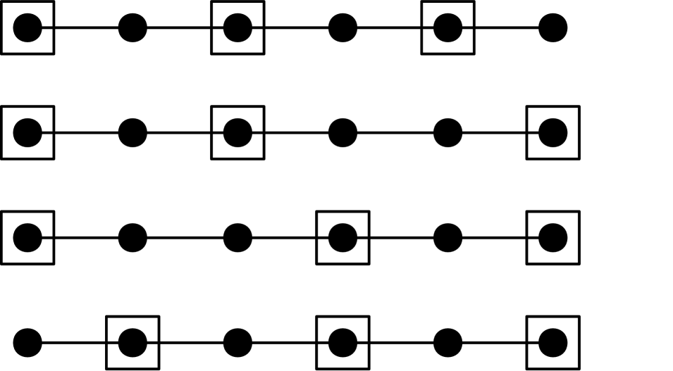
(a) Maximum independent sets in $P_{6}$ are denoted by the squared vertices.

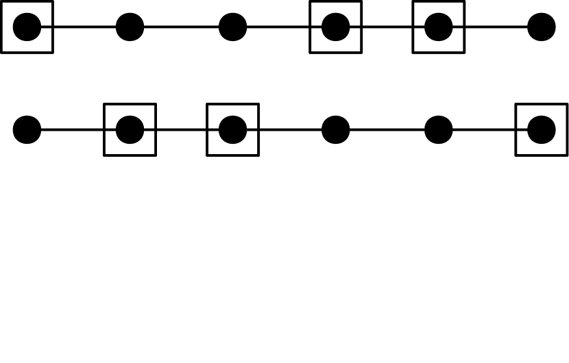
(b) Minimum solid-locating-dominating codes in $P_{6}$ are denoted by the squared vertices.

Figure 3: Maximum independent sets and minimum solid-locating-dominating codes are different.

4 Cartesian products and ladders

In this section, we consider self-location-domination and solid-location-domination in the Cartesian product of graphs. The Cartesian product of graphs $G=(V(G),E(G))$ and $H=(V(H),E(H))$ is $G\square H=(V(G)\times V(H),E)$ where $(u,v)(u^{\prime},v^{\prime})\in E$ if and only if $u=u^{\prime}$ and $vv^{\prime}\in E(H)$ or $uu^{\prime}\in E(G)$ and $v=v^{\prime}$. We begin by presenting a theorem which gives lower and upper bounds for the self-location-domination and the solid-location-domination numbers for Cartesian products. Then we proceed by studying these numbers more closely in the Cartesian products $P_{n}\Box P_{2}$, where $P_{k}$ denotes a path with $k$ vertices. Using these results concerning $P_{n}\Box P_{2}$ and some other previously known ones for the Cartesian product of two complete graphs (see [16]), we are able to show that most of the obtained lower and upper bounds can be attained.

Theorem 31.

We have

• $\max\{\gamma^{SLD}(G),\gamma^{SLD}(H)\}\leq\gamma^{SLD}(G\Box H)\leq\min\{|V(H)|\gamma^{SLD}(G),|V(G)|\gamma^{SLD}(H)\}$ and

• $\max\{\gamma^{DLD}(G),\gamma^{DLD}(H)\}\leq\gamma^{DLD}(G\Box H)\leq\min\{|V(H)|\gamma^{DLD}(G),|V(G)|\gamma^{DLD}(H)\}$.

Proof.

(i) Let us first show the upper bound on $\gamma^{SLD}(G\Box H).$ Without loss of generality, we may assume that $|V(H)|\gamma^{SLD}(G)\leq|V(G)|\gamma^{SLD}(H)$. Let $C$ be a self-locating-dominating code in $G$ attaining $\gamma^{SLD}(G).$ Denote $D=\{(c,v)\mid c\in C,v\in V(H)\}$. Clearly, $|D|=|V(H)|\gamma^{SLD}(G).$ We will show that $D$ is self-locating-dominating in $G\Box H.$ We denote, for any $h\in V(H)$, the set $\{(u,h)\mid u\in V(G)\}$ by $L_{h}$ and we call it a layer. Observe that for any vertices $(u_{1},h)$ and $(u_{2},h)$ ($u_{1}\neq u_{2}$) in the same layer $L_{h}$ we have $N[(u_{1},h)]\cap N[(u_{2},h)]\subseteq L_{h}$. Let $x$ be any non-codeword in $G\Box H$, say $x=(u,h)\in L_{h}$ for some $h$ and $u\in V(G)\setminus C$. Now the codewords in $I(G\Box H;x)$ all belong to $L_{h}$. Since $C$ is self-locating-dominating in $G$, we get (by the previous observation) that

$$\bigcap_{c\in I(G\Box H;x)}N[c]=\{x\}.$$

Next we consider the lower bound on $\gamma^{SLD}(G\Box H)$. Without loss of generality, say $\gamma^{SLD}(G)\geq\gamma^{SLD}(H).$ Let $D$ be a self-locating-dominating code in $G\Box H$ of cardinality $\gamma^{SLD}(G\Box H).$ Denote by $C(\subseteq V(G))$ the set which is obtained by collecting all the first coordinates from $D$. We claim that $C$ is self-locating-dominating in $G$. Let $u\in V(G)$ be a non-codeword with respect to $C.$ This implies that the vertices $(u,h)$ are non-codewords with respect to $D$ for all $h\in V(H)$ and hence, $I((u,h))\subseteq L_{h}$. Since $D$ is self-locating-dominating, we know that for any layer $L_{h}$ the neighbourhoods of the codewords in $I(G\Box H,D;(u,h))$ intersect uniquely in $(u,h)$. Because the first coordinates of the codewords in $I(G\Box H,D;(u,h))$ belong to $I(G,C;u)$, we obtain

$$\bigcap_{c\in I(G,C;u)}N[c]=\{u\}.$$

Thus $C$ is self-locating-dominating and the claim follows by noticing that $|C|\geq\gamma^{SLD}(G).$

(ii) We can again assume without loss of generality that $|V(H)|\gamma^{DLD}(G)\leq|V(G)|\gamma^{DLD}(H)$. Let $C$ be a solid-locating-dominating code in $G$ attaining $\gamma^{DLD}(G)$ and denote again $D=\{(c,v)\mid c\in C,v\in V(H)\}$. In order to verify that $D$ is solid-locating-dominating in $G\Box H$, we show that $I(D;x)\setminus I(D;y)$ is non-empty for any distinct non-codewords $x,y\in V(G\Box H).$ Denote $x=(u,h)$ and $y=(v,h^{\prime})$ for some $u,v\in V(G)$ and $h,h^{\prime}\in V(H).$ If $h=h^{\prime}$, then we are done, since $C$ is solid-locating-dominating. If $h\neq h^{\prime}$, then the claim follows from the fact that $I(D;x)$ contains a codeword in the layer $L_{h}$ and $I(D;y)$ cannot contain that codeword (since $x$ and $y$ are non-codewords).

The proof of the lower bound is again similar — let $D$ be a solid-locating-dominating code in $G\Box H$ of cardinality $\gamma^{DLD}(G\Box H)$ and $C$ be a set obtained from its first coordinates. Now let $u\in V(G)$ and $v\in V(G)$ be non-codewords with respect to $C$. This implies that the vertices $(u,h)$ and $(v,h^{\prime})$ are non-codewords with respect to $D$ for all $h,h^{\prime}\in H.$ Since $D$ is solid-locating-dominating, we must have that $I(D;(u,h))\setminus I(D;(v,h))$ contains a codeword $(c,h)$ of $D$ in the layer $L_{h}$. Therefore, $c\in I(C;u)\setminus I(C;v)$ in $G$ and we are done. ∎

Remark 32.

Due to Corollary 15, for any complete graph $K_{m}$, we have $\gamma^{SLD}(K_{m})=m$. Moreover, it has been shown in [16] that $\gamma^{SLD}(K_{m}\Box K_{n})=m$ for $m\geq 2n$. Therefore, the lower bound of Case (i) of the previous theorem can be attained.

In what follows, we focus on the self-location-domination and solid-location-domination numbers in the Cartesian product of paths $P_{n}$ and $P_{2}$. Using these results, we are able to show that the upper bounds in Cases (i) and (ii) can be attained.

The Cartesian product of the paths $P_{n}$ and $P_{2}$ will be called the ladder (graph) of length $n$. Furthermore, we use the following notation for the vertex sets of $P_{n}$ and $P_{2}$: $V(P_{n})=\{v_{1},v_{2},v_{3},\dots v_{n}\}$ and $V(P_{2})=\{1,2\}$, and so the vertex set of the Cartesian product $P_{n}\Box P_{2}$ is $V(P_{n}\Box P_{2})=\{(v_{i},j)\colon 1\leq i\leq n,\ 1\leq j\leq 2\}$ (see Figure 4).

Figure 4: The ladder $P_{n}\Box P_{2}$.

The following notation will be useful in this section. Let $1\leq r\leq n$ be an integer. Now $P_{r}\Box P_{2}$ is the subgraph of $P_{n}\Box P_{2}$ induced by the vertex set $\{(v_{i},j)\colon 1\leq i\leq r,\ 1\leq j\leq 2\}$ (see Figure 5(a)), which is a ladder of length $r$. On the other hand, for an integer $0\leq s\leq n-1$, $P_{n-s}\Box P_{2}$ is the subgraph of $P_{n}\Box P_{2}$ induced by $\{(v_{i},j)\colon s+1\leq i\leq n,\ 1\leq j\leq 2\}$ (see Figure 5(b)), which is a ladder of length $n-s$.

(a) Subgraph $P_{r}\Box P_{2}$.

(b) Subgraph $P_{n-s}\Box P_{2}$.

Figure 5: Induced subgraphs in $P_{n}\Box P_{2}$.

We begin by computing the self-location-domination number of ladders. To this end, we will use the relationship between self-locating-dominating codes and $2$-dominating sets that we showed in Lemma 23. It is known that $\gamma_{2}(P_{n}\Box P_{2})=n$ (see [20, 23]) for $n\geq 2$ and $\gamma_{2}(P_{1}\Box P_{2})=2$. In the next lemma, we prove an additional property of optimal $2$-dominating sets that will be useful to our purpose.

Lemma 33.

Let $n\geq 2$ be an integer and let $C\subseteq V(P_{n}\Box P_{2})$ be a $2$-dominating set such that $|C|=n$. Then we have $\{(v_{1},1),(v_{1},2)\}\nsubseteq C$.

Proof.

There are exactly two $2$-dominating sets in $P_{2}\Box P_{2}$ with two vertices (see Figure 6(a)) and exactly two $2$-dominating sets in $P_{3}\Box P_{2}$ with three vertices (see Figure 6(b)). Therefore, the statement is clearly true for $n=2$ and $n=3$.

(a) $2$-dominating sets with two vertices in $P_{2}\Box P_{2}$.

(b) $2$-dominating sets with three vertices in $P_{3}\Box P_{2}$.

Figure 6: Squared vertices are in the $2$-dominating set.

We now proceed by induction on $n$. Assume the statement is true for $k<n$, $n\geq 4$, and let $C$ be a $2$-dominating set of $P_{n}\Box P_{2}$ such that $|C|=n$. Suppose to the contrary that $\{(v_{1},1),(v_{1},2)\}\subseteq C$, then, because $C$ has $n$ elements, there exists $i\in\{2,\dots,n\}$ such that $(v_{i},1),(v_{i},2)\notin C$. Note that $i<n$, because $C$ is $2$-dominating. Now $\{(v_{i-1},1),(v_{i-1},2),(v_{i+1},1),(v_{i+1},2)\}\subseteq C$ to keep the $2$-domination.

Consider the induced subgraphs $G_{1}=P_{i-1}\Box P_{2}$ and $G_{2}=P_{n-i}\Box P_{2}$. It is clear that $C\cap V(G_{1})$ and $C\cap V(G_{2})$ are $2$-dominating sets in $G_{1}$ and $G_{2}$, respectively. Moreover, they satisfy $(v_{i-1},1),(v_{i-1},2)\in C\cap V(G_{1})$ and $(v_{i+1},1),(v_{i+1},2)\in C\cap V(G_{2})$.

Suppose that $i-1\geq 2$ and $n-i\geq 2$. By the inductive hypothesis $|C\cap V(G_{1})|\geq(i-1)+1=i$ and $|C\cap V(G_{2})|\geq(n-i)+1$. Therefore, $|C|\geq n+1$, which is a contradiction. Assume now that $i-1=1$ and $n-i=n-2$. In this case $|C\cap V(G_{1})|=2$ and, by the inductive hypothesis, $|C\cap V(G_{2})|\geq(n-2)+1=n-1$. Again $|C|\geq n+1$, a contradiction. The remaining case, $i-1=n-2$ and $n-i=1$, is similar to the previous one. Therefore, $\{(v_{1},1),(v_{1},2)\}\nsubseteq C$ as desired. ∎

This property gives that self-locating-dominating codes of ladders $P_{n}\Box P_{2}$ are non-optimal $2$-dominating sets for $n\geq 2$.

Lemma 34.

Let $C$ be a self-locating-dominating code in $P_{n}\Box P_{2}$ with $n\geq 2$. Then $(v_{1},1),(v_{1},2),\linebreak(v_{n},1),(v_{n},2)\in C$ and $|C|\geq n+1$.

Proof.

By Lemma 23, $C$ is a $2$-dominating set in $P_{n}\Box P_{2}$. Hence, we have $|C|\geq n$. Suppose that $(v_{1},1)\notin C$. Now $(v_{1},2),(v_{2},1)\in C$ and $(v_{2},2)\in\bigcap_{c\in I((v_{1},1))}N[c]$, which is not possible for a self-locating-dominating code. So $(v_{1},1)\in C$ and analogously $(v_{1},2),(v_{n},1),(v_{n},2)\in C$. Using Lemma 33, we obtain that $|C|\geq n+1$. ∎

We can now compute the exact self-location-domination numbers of ladders.

Theorem 35.

Let $n\geq 2$ be an integer. Then

$$\gamma^{SLD}(P_{n}\Box P_{2})=\left\{\begin{array}[]{ll}n+1&\hbox{if $n$ is odd;}\\ n+2&\hbox{if $n$ is even.}\end{array}\right.$$

Proof.

If $n=2k+1$, $k\geq 1$, then the set $\{(v_{2i+1},1),(v_{2i+1},2)\colon 0\leq i\leq k\}$ (see Figure 7) is a self-locating-dominating code with $2(k+1)=n+1$ vertices. Thus, Lemma 34 gives $\gamma^{SLD}(P_{2k+1}\Box P_{2})=(2k+1)+1$.

Figure 7: Squared vertices form an optimal self-locating-dominating code in $P_{2k+1}\square P_{2}$.

Assume now that $n=2k$, $k\geq 1$. We will prove that $\gamma^{SLD}(P_{2k}\Box P_{2})\geq 2k+2$, by induction on $k$. Clearly, $\gamma^{SLD}(P_{2}\Box P_{2})=4$ (by the proof of Lemma 34). Assume that the statement is true for $r<k$, $k\geq 2$, and let $C\subseteq V(P_{2k}\Box P_{2})$ be a self-locating-dominating code. Suppose that $\{(v_{i},1),(v_{i},2)\}\cap C\neq\emptyset$ for every $i\in\{1,2,\dots,2k\}$. By Lemma 34, $(v_{1},1),(v_{1},2),(v_{2k},1),$ $(v_{2k},2)\in C$. So $|C|\geq 2k+2$.

Suppose now that there exists $i\in\{2,\dots,2k-1\}$ such that $(v_{i},1),(v_{i},2)\notin C$. Since $C$ is also a $2$-dominating set, we obtain that $\{(v_{i-1},1),(v_{i-1},2),(v_{i+1},1),(v_{i+1},2)\}\subseteq C$. Consider the induced subgraphs $G_{1}=P_{i-1}\Box P_{2}$ and $G_{2}=P_{2k-i}\Box P_{2}$, with self-locating-dominating codes $C\cap V(G_{1})$ and $C\cap V(G_{2})$, respectively. Note that $(i-1)+(2k-i)$ is odd. Let us assume that $i-1$ is odd and $2k-i$ is even (the other case is analogous). For $i-1$ odd, we know that $|C\cap V(G_{1})|\geq(i-1)+1$ (this holds also for $i=2$) and when $2k-i$ is an even number, by the inductive hypothesis, $|C\cap V(G_{2})|\geq(2k-i)+2$. This gives $|C|\geq 2k+2$.

Finally the set $\{(v_{2i+1},1),(v_{2i+1},2)\colon 0\leq i\leq k-1\}\cup\{(v_{2k},1),(v_{2k},2)\}$ (see Figure 8) is a self-locating-dominating code of $P_{2k}\Box P_{2}$ with $2k+2$ vertices and therefore $\gamma^{SLD}(P_{2k}\Box P_{2})=2k+2$. ∎

Figure 8: Squared vertices form an optimal self-locating-dominating code in $P_{2k}\square P_{2}$.

Remark 36.

Recall that we have $\gamma^{SLD}(P_{n})=\gamma_{2}(P_{n})=\lceil(n+1)/2\rceil$ by Corollary 25. Notice then that, whether $n$ is even, with $n=2k$, or odd, with $n=2k+1$, we have shown that $\gamma^{SLD}(P_{n}\Box P_{2})=2k+2=2(k+1)=|V(P_{2})|\gamma^{SLD}(P_{n})$. Therefore, the upper bound of Case (i) of Theorem 31 is attained for both even and odd $n$.

We now focus on the solid-location-domination number of ladders.

Proposition 37.

Let $n\geq 1$ be an integer and $C\subseteq V(P_{n}\Box P_{2})$ be a solid-locating-dominating code. Then $|C|\geq n.$

Proof.

The statement is clearly true for $n=1$ and $n=2$. Assume now that $n\geq 3$ and the claim is true for every $k<n$. Let $C\subseteq V(P_{n}\Box P_{2})$ be a solid-locating-dominating code and suppose to the contrary that $|C|<n$. Then there exists $i\in\{1,2,\dots,n\}$ such that $(v_{i},1),(v_{i},2)\notin C$.

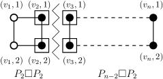
Figure 9: Squared vertices are in $C$ and white vertices are not in $C$.

Firstly suppose that $(v_{1},1),(v_{1},2)\notin C$, then using the fact that $C$ is a solid-locating-dominating code we obtain that $(v_{2},1),(v_{2},2),(v_{3},1),(v_{3},2)\in C$. Consider the induced subgraphs $G_{1}=P_{2}\Box P_{2}$ and $G_{2}=P_{n-2}\Box P_{2}$. Clearly both $C\cap V(G_{1})$ and $C\cap V(G_{2})$ are solid-locating-dominating codes in $G_{1}$ and $G_{2}$ respectively (see Figure 9). Moreover, $|C\cap V(G_{1})|=2$ and by the inductive hypothesis $|C\cap V(G_{2})|\geq n-2$. Hence, we have $|C|\geq n$ (a contradiction). Therefore, we may assume that $1<i$ and, with the same reasoning, that $i<n$.

Assume now that $(v_{i+1},1),(v_{i+1},2)\notin C$. Consequently, the vertices $(v_{i-1},1)$, $(v_{i-1},2)$, $(v_{i+2},1)$ and $(v_{i+2},2)$ belong to $C$. Consider the induced subgraphs $G_{1}=P_{i}\Box P_{2}$ and $G_{2}=P_{n-i}\Box P_{2}$ with solid-locating-dominating codes $C\cap V(G_{1})$ and $C\cap V(G_{2})$, respectively (see Figure 10(a)). By the inductive hypothesis $|C\cap V(G_{1})|\geq i$ and $|C\cap V(G_{2})|\geq n-i$, so $|C|\geq n$, which is a contradiction. A similar argument can be used if $(v_{i-1},1),(v_{i-1},2)\notin C$.

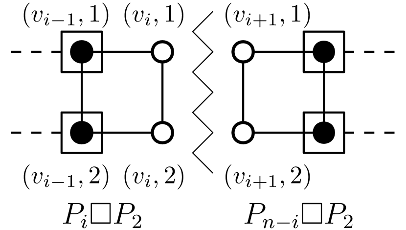
(a)

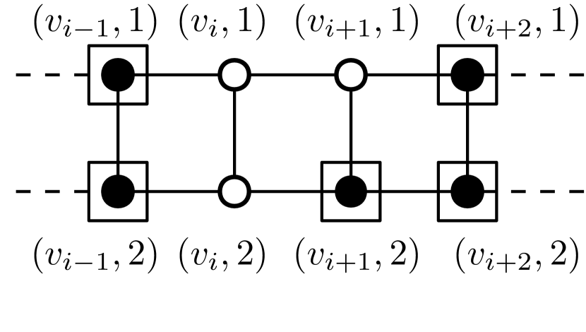
(b)

Figure 10: Squared vertices are in $C$ and white vertices are not in $C$.

Suppose that $(v_{i+1},1)\notin C$ and $(v_{i+1},2)\in C$. Clearly, $i+2\leq n$ and $(v_{i+2},1)\in C$ because otherwise $I((v_{i+1},1))\subseteq I((v_{i},2))$. Moreover, $(v_{i+2},2)\in C$ because otherwise $I((v_{i+1},1))\subseteq I((v_{i+2},2))$. Furthermore, $(v_{i-1},1)\in C$ since $I((v_{i},1))\neq\emptyset$ and $(v_{i-1},2)\in C$ as otherwise $I((v_{i},1))\subseteq I((v_{i-1},2))$. Hence, there are two pairs of codewords $\{(v_{i-1},1),(v_{i-1},2)\}$ and $\{(v_{i+2},1),(v_{i+2},2)\}$ such that the pair of non-codewords $\{(v_{i},1),(v_{i},2)\}$ is between them (see Figure 10(b)).

We have stated that there cannot be a pair of non-codewords at the beginning or the end of the ladder. Furthermore, we may assume that there are no consecutive pairs of non-codewords and, if there is a pair of non-codewords $(v_{i},1),(v_{i},2)$, then there are two pairs of codewords $\{(v_{j},1),(v_{j},2)\}$ and $\{(v_{j^{\prime}},1),(v_{j^{\prime}},2)\}$, $j<i<j^{\prime}$, such that if for some $i^{\prime}$, $j<i^{\prime}<j^{\prime}$, we have $(v_{i^{\prime}},1),(v_{i^{\prime}},2)\not\in C$, then $i^{\prime}=i$. Hence, the number of vertex pairs such that $\{(v_{j},1),(v_{j},2)\}\subseteq C$ is greater or equal to the number of vertex pairs $(v_{i},1),(v_{i},2)\not\in C$ and thus, we have $|C|\geq n$. ∎

We can finally determine the exact solid-location-domination numbers of all ladders.

Corollary 38.

If $n\geq 1$ is an integer, then $\gamma^{DLD}(P_{n}\Box P_{2})=n$.

Proof.

The set $C=\{(v_{i},1)\colon 1\leq i\leq n\}$ is a solid-locating-dominating code in $P_{n}\Box P_{2}$ with $n$ elements since $I((v_{i},2))=\{(v_{i},1)\}$. So, $\gamma^{DLD}(P_{n}\Box P_{2})\leq n$. The reverse inequality comes from Proposition 37. ∎

Remark 39.

Recall that we have $\gamma^{DLD}(P_{n})=\beta(P_{n})=\lceil n/2\rceil$ by Corollary 29. Notice that, if $n$ is an even number, then $\gamma^{DLD}(P_{n}\Box P_{2})=2\cdot\tfrac{n}{2}=|V(P_{2})|\gamma^{DLD}(P_{n})$. Therefore, the upper bound shown in Case (ii) of Theorem 31 is attained in this case.

5 Realization theorems

In this section, we consider location-domination, self-location-domination and solid-location-domination numbers; in particular, we study what are the values the location-domination number can simultaneously have with the self-location-domination or the solid-location-domination number in a graph. Similar types of questions have been previously studied in [5] regarding various values such as domination number, location-domination number and metric dimension. In the following theorem, we characterize which values of location-domination and self-location-domination numbers can be simultaneously achieved in a graph.

Theorem 40.

Let $a$ and $b$ be positive integers. Then there exists a graph $G$ such that $a=\gamma^{LD}(G)$ and $b=\gamma^{SLD}(G)$ if and only if we have

$$0\leq b-a\leq 2^{a}-1.$$

Proof.

We cannot have $a>b$ since each self-locating-dominating code is also locating-dominating. We also cannot have $b>a+2^{a}-1$ since we can have at most $a+2^{a}-1$ vertices in a graph with locating-dominating code of cardinality $a$ by [25]. Hence, $b-a$ is in the claimed interval. Based on the difference $b-a$, the proof divides into the following cases: (i) $a=b$, (ii) $b-a=1$, (iii) $a=2$ and $b=4$ or $b=5$, (iv) $2\leq b-a\leq 2^{a}-2$ and $a\geq 3$, and (v) the extremal case $a\geq 3$ and $b-a=2^{a}-1$.

(i) Let us first study the case $a=b$. We can now consider the discrete graph $G$, that is, the graph with no edges, of order $a$ and we have $\gamma^{SLD}(G)=\gamma^{LD}(G)$.

(ii) Let us then study the case $b=a+1$. We can consider graph $G$ of order $b$ with one edge and we have $\gamma^{SLD}(G)=\gamma^{LD}(G)+1$.

(iii) Let us then study the case $a=2$ and $b=4$. We immediately notice that these numbers are realized in the graph of Figure 11(a). The case $a=2$ and $b=5$ is given in the graph of Figure 11(b).

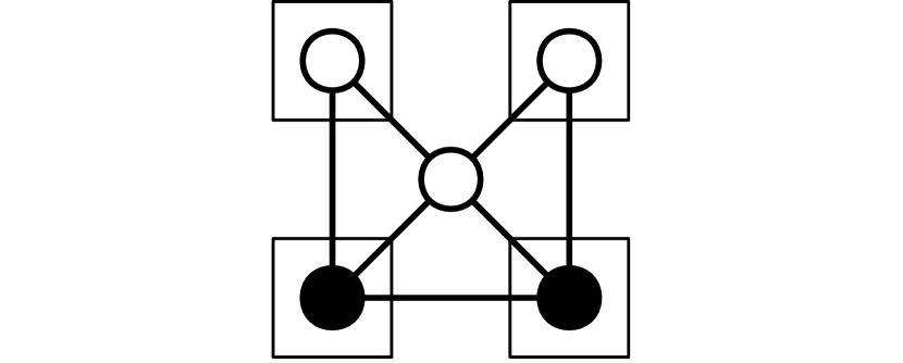
(a) $\gamma^{LD}(G)=2,\gamma^{SLD}(G)=4$.

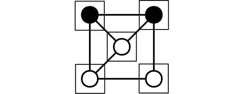
(b) $\gamma^{LD}(G)=2,\gamma^{SLD}(G)=5$.

Figure 11: Black vertices are in an optimal locating-dominating code and squared vertices are in an optimal self-locating-dominating code.

(iv) Let us then study the case $2\leq b-a\leq 2^{a}-2$ and $a\geq 3$. There is an integer $k\in\mathbb{Z}$ such that $2^{k-1}-2<b-a\leq 2^{k}-2$. Notice that $2\leq k\leq a$. Let us have $K=\{v_{i}\mid 1\leq i\leq k\}$, $K^{\prime}=\{v_{i}\mid k+1\leq i\leq a\}$, $P=\{u_{i}\mid 1\leq i\leq b+1-a\}$ and $V=K\cup K^{\prime}\cup P$. We have $|V|=b+1$. Let us connect $u_{1}$ to each vertex in $V$ and each vertex $u_{i}$, $2\leq i\leq k+1$ to a single vertex $v_{j}$, $j=i-1$. Indeed, the latter edges are possible since for any $k\geq 3$ we have $|P|\geq 2^{k-1}-1+1\geq k+1$ and if $k=2$, then $b-a=2$ and $|P|\geq 3$. Let us further connect each other vertex in $P$ to some proper non-empty subset of vertices in $K$ in such a manner that no two vertices in $P$ have the same neighbourhood in $K$. This choice of non-identical neighbourhoods is possible since we have $|P|\leq 2^{|K|}-1=2^{k}-1$. A graph $G$ with $k=4$ and $|V|=16$ is shown in the Figure 12.

Let us first consider self-location-domination in $G$. There are $b$ forced codewords in a self-locating-dominating code since we have $N(v)\subseteq N[u_{1}]$ for each $v\in V$. Hence, we have $\gamma^{SLD}(G)\geq b$ and $V\setminus\{u_{1}\}$ is a self-locating-dominating code since $I(u_{2})\cap I(u_{3})=\{u_{1}\}$ and thus, $\gamma^{SLD}(G)=b$.

Let us then consider location-domination in $G$. We can choose each vertex in $K\cup K^{\prime}$ as a codeword and have a locating-dominating code of size $a$. Let us show that $\gamma^{LD}(G)\geq a$. We have $N[u_{j+1}]=\{u_{1},u_{j+1},v_{j}\}$ for each $1\leq j\leq k$. Hence, if $v_{j}$ and $v_{j}^{\prime}$ in $K$ are non-codewords, then at least two of vertices $u_{j+1}$, $u_{j^{\prime}+1}$ and $u_{1}$ are codewords. Furthermore, by the same idea, if we have $t$ non-codewords in $K$, then there are at least $t$ codewords in $P$. Hence, we have at least $k$ codewords in $K\cup P$. Since we have $N(v_{i})=\{u_{1}\}$ for each vertex $v_{i}$ in $K^{\prime}$, we have at least $|K^{\prime}|$ codewords in $K^{\prime}\cup\{u_{1}\}$. If $u_{1}$ is a non-codeword, then it is immediate that we have $|K|+|K^{\prime}|=a$ codewords in $G$. Hence, we may assume that $u_{1}$ is a codeword. If all the vertices $v_{k+1},v_{k+2},\ldots,v_{a}$ are codewords, then we are again immediately done. Moreover, by the previous observations at most one of the vertices can be a non-codeword. Hence, we may assume that there exists a unique non-codeword $v_{y}$, $y\geq k+1$. Now we have $I(v_{y})=\{u_{1}\}$. Therefore, for any $1\leq j\leq k$ at least one of $v_{j}$ and $u_{j+1}$ is a codeword as otherwise $I(u_{j+1})=\{u_{1}\}=I(v_{y})$ (a contradiction). Thus, there exist $|K|=k$ codewords in $K\cup P\setminus\{u_{1}\}$. Hence, in all the cases, we have $\gamma^{LD}(G)\geq a$.

(v) Let us finally study the extremal case $a\geq 3$ and $b-a=2^{a}-1$. Let us consider graph $G=(V,E)$. Let us have $K=\{v_{i}\mid 1\leq i\leq a\}$, $P=\{u_{i}\mid 1\leq i\leq b-a\}$ and $V=K\cup P$. Let us connect

1. $v_{1}$ to $v_{i}$ for each $2\leq i\leq a$

2. $u_{1}$ to $v_{i}$ for each $1\leq i\leq a$

3. $u_{i}$, $2\leq i\leq a$, to $v_{1}$ and $v_{i}$

4. $u_{i}$, $a+1\leq i\leq b-a$, to some non-empty subset of vertices of $K$ in such a manner that no two vertices of $P$ have the same neighbourhood in $K$. This is possible since $|P|\leq 2^{|K|}-1$.

5. $u_{1}$ to $u_{i}$, $2\leq i\leq b-a$, if $u_{i}\in N(v_{1})$

6. $u_{i}$, $2\leq i\leq a$, to $u_{j}$, $a+1\leq j\leq b-a$, if $u_{j}\in N(v_{i})$.

Since we have $2^{a}+a-1$ vertices in the graph, we have $\gamma^{LD}(G)\geq a$. On the other hand, we can choose $K$ as an optimal locating-dominating code, since if $u,u^{\prime}\in P$, then $N(u)\cap K\neq N(u^{\prime})\cap K$ and $|K|=a$. In order to prove that $\gamma^{SLD}(G)=b=|V|$, we have to show that each vertex of the graph is a forced codeword. By Theorem 9, it suffices to show that for each vertex $v\in V$ there exists another vertex $v^{\prime}$ such that $N(v)\subseteq N[v^{\prime}]$. Indeed, it is straightforward to verify that $N[v_{i}]=N[u_{i}]$ for $1\leq i\leq a$ and $N(u_{i})\subseteq N[u_{1}]$ for $a+1\leq i\leq b-a$. Thus, the claim follows. ∎

Figure 12: Graph $G$ with $k=4$, $\gamma^{LD}(G)=6$ and $\gamma^{SLD}(G)=15$. Squared vertices are codewords in an optimal self-locating-dominating code and gray vertices are codewords in an optimal locating-dominating code.

In the following theorem, we proceed by characterizing which values of location-domination and solid-location-domination numbers can be simultaneously achieved in a graph.

Theorem 41.

Let $a$ and $b$ be positive integers. Then there exists a graph $G$ such that $a=\gamma^{LD}(G)$ and $b=\gamma^{DLD}(G)$ if and only if we have

$$0\leq b-a\leq 2^{a}-1-\binom{a}{\left\lceil\frac{a}{2}\right\rceil}.$$

Proof.

Let us have a locating-dominating code $C_{LD}$ of cardinality $a$ in $G=(V,E)$. Then all the $|V|-a$ non-codewords $u\in V$ have different and non-empty sets $I(C_{LD};u)$. Hence, we have $|V|\leq 2^{a}-1+a$. Denote $R=\left\{v\in V\mid|N[v]\cap C_{LD}|=\left\lceil\frac{a}{2}\right\rceil,v\not\in C_{LD}\right\}$. Clearly, $0\leq|R|\leq\binom{a}{\left\lceil\frac{a}{2}\right\rceil}$ and there are at most $2^{a}-1+a-\binom{a}{\left\lceil\frac{a}{2}\right\rceil}$ vertices in $V\setminus R$ (as the $I$-sets of the non-codewords have to be non-empty and unique). Denote then $D=V\setminus R$. Now for any distinct pair of vertices $v,w\in R$ we have $I(D;v)\not\subseteq I(D;w)$ because $C_{LD}\subseteq D$ and $|I(C_{LD};v)|=|I(C_{LD};w)|=\lceil a/2\rceil$. Therefore, we have $b=\gamma^{DLD}(G)\leq|D|\leq 2^{a}-1+a-\binom{a}{\left\lceil\frac{a}{2}\right\rceil}$. Thus, we obtain that $b-a\leq 2^{a}-1-\binom{a}{\left\lceil\frac{a}{2}\right\rceil}$.

Let us first consider the situation $a=b$ and a graph $G=(V,E)$. We notice that this is possible by assuming that $G$ is the star with $a$ pendant vertices. Let us then assume that $a<b$ and let us have $k\in\mathbb{Z}_{+}$ such that $2^{k-1}-1-\binom{k-1}{\left\lceil\frac{k-1}{2}\right\rceil}<b-a\leq 2^{k}-1-\binom{k}{\left\lceil\frac{k}{2}\right\rceil}$. Since $2^{k}-1-\binom{k}{\left\lceil\frac{k}{2}\right\rceil}$ is an increasing function on $k$ when $k>0$ and it gains value $1$ when $k=2$, each value of difference $b-a$ is linked to a unique value of $k$. Since the function gives $0$ when $k=1$, we can assume that $k\geq 2$. Let us have $K=\{v_{i}\mid 1\leq i\leq k\}$, $K^{\prime}=\{v_{i}\mid k+1\leq i\leq a\}$, $P=\left\{u_{i}\mid 1\leq i\leq b-a+\binom{k}{\left\lceil\frac{k}{2}\right\rceil}\right\}$ and $V=K\cup K^{\prime}\cup P$. We have $|V|=b+\binom{k}{\left\lceil\frac{k}{2}\right\rceil}$. Let us connect

1. $v_{i}$ to $v_{j}$ for each $1\leq i<j\leq a$ forming the complete graph $K_{a}$,

2. $u_{1}$ to $v_{i}$ for each $1\leq i\leq a$,

3. each $u_{i}$, $2\leq i\leq\binom{k}{\left\lceil\frac{k}{2}\right\rceil}+1$, to $\left\lfloor\frac{k}{2}\right\rfloor$ vertices in $K$ in such a manner that all of these vertices have different open neighbourhoods,

4. each $u_{i}$, $\binom{k}{\left\lceil\frac{k}{2}\right\rceil}+2\leq i\leq\binom{k}{\left\lceil\frac{k}{2}\right\rceil}+k+1$, to vertex $v_{j}$ with $j=i-\binom{k}{\left\lceil\frac{k}{2}\right\rceil}-1$ when $k\geq 4$ (and no vertices are connected if $2\leq k\leq 3$) and

5. each other vertex $u_{i}\in P$ to some non-empty subset of vertices in $K$ in such a manner that no two vertices of $P$ have the same neighbourhood in $K$.

Denote the graph constructed above by $G$. Step $3$ is possible since $\binom{k}{\left\lceil\frac{k}{2}\right\rceil}=\binom{k}{\left\lfloor\frac{k}{2}\right\rfloor}$ and $|P|\geq\binom{k}{\left\lceil\frac{k}{2}\right\rceil}+1$. Furthermore, because $k\geq 2$, $u_{1}$ has different neighbourhood in $K$ (compared to the vertices of Step 3). Step $4$ is possible since

$$|P|\geq 2^{k-1}-1-\binom{k-1}{\left\lceil\frac{k-1}{2}\right\rceil}+\binom{k}{\left\lceil\frac{k}{2}\right\rceil}+1=\sum_{i=0}^{k-1}\binom{k-1}{i}-\binom{k-1}{\left\lceil\frac{k-1}{2}\right\rceil}+\binom{k}{\left\lceil\frac{k}{2}\right\rceil}\geq\binom{k}{\left\lceil\frac{k}{2}\right\rceil}+k+1$$

when $k\geq 4$. However, when $k=2$ or $k=3$, we have $\left\lfloor\frac{k}{2}\right\rfloor=1$ and thus, by step $3$, also in these cases for each vertex $v\in K$ there exists a vertex of $P$ such that it has only $v$ in its neighbourhood. Step $5$ is possible since we have $|P|\leq 2^{|K|}-1=2^{k}-1$.

Let us first show that the location-domination number of $G$ is equal to $a$. We can now choose $K\cup K^{\prime}$ as a locating-dominating code of size $a$ since each vertex in $P$ has its open neighbourhood with a unique and non-empty intersection with $K$. Furthermore, each vertex in $K^{\prime}\cup\{u_{1}\}$ has the same closed neighbourhood and hence, we can have at most one non-codeword among them. Since each vertex $v_{j}\in K$ neighbours a vertex $u_{i}$ such that $N(u_{i})=\{v_{j}\}$ for some $j$ and $i$, we have $v_{j}$ or $u_{i}$ in the code and hence, we have at least $|K|+|K^{\prime}|=a$ codewords. Thus, $\gamma^{LD}(G)=a$.

Let us then show that $\gamma^{DLD}(G)=b$. We can choose as our solid-locating-dominating code $C$ the vertex set containing all vertices except for $u_{i}$ for $2\leq i\leq\binom{k}{\left\lceil\frac{k}{2}\right\rceil}+1$. We have $|C|=b$ (as $|V|=b+\binom{k}{\lceil k/2\rceil}$) and if $v,v^{\prime}\not\in C$, then $|N(v)\cap K|=|N(v^{\prime})\cap K|=\left\lfloor\frac{k}{2}\right\rfloor$ and $N(v)\cap K\neq N(v^{\prime})\cap K$ and hence, $C$ is a solid-locating-dominating code. In order to show that $\gamma^{DLD}(G)\geq b$, let $X$ be a solid-locating-dominating code in $G$. Observe that if a vertex $v_{h}\in K^{\prime}\cup K$ does not belong to $X$, then each vertex in $P$ is in the code since for $u_{i}\in P$ we have $N(u_{i})\subseteq K^{\prime}\cup K\subseteq N[v_{h}]$. Moreover, since we have $N[v^{\prime}]\subseteq N[v]$ when $v^{\prime}\in K^{\prime}$ and $v\in K^{\prime}\cup K$, we can have at most one non-codeword in $K^{\prime}$ and only if there are no non-codewords in $K$. Therefore, we may assume that $K\cup K^{\prime}\subseteq X$ since otherwise we would have at least $|P|+|K^{\prime}|=b+\binom{k}{\left\lceil\frac{k}{2}\right\rceil}-k\geq b$ codewords because $\binom{k}{\left\lceil\frac{k}{2}\right\rceil}\geq k$. Furthermore, due to the Sperner’s theorem and the independence of the set $P$, we can choose at most $\binom{k}{\left\lceil\frac{k}{2}\right\rceil}$ vertices in $P$ in such a manner that none of their neighbourhoods is contained within another. This gives $\gamma^{DLD}(G)\geq b$.∎

References

- [1] C. Berge. Graphs and Hypergraphs. North-Holland, Amsterdam, 1976.
- [2] M. Blidia, M. Chellali, and O. Favaron. Independence and 2-domination in trees. Australas. J. Combin., 33:317–327, 2005.
- [3] M. Blidia, M. Chellali, O. Favaron, and N. Meddah. On -independence in graphs with emphasis on trees. Discrete Math., 307(17-18):2209–2216, 2007.
- [4] M. Blidia, O. Favaron, and R. Lounes. Locating-domination, -domination and independence in trees. Australas. J. Combin., 42:309–316, 2008.
- [5] J. Cáceres, C. Hernando, M. Mora, I. M. Pelayo, and M. L. Puertas. Locating-dominating codes: bounds and extremal cardinalities. Appl. Math. Comput., 220:38–45, 2013.
- [6] V. Chvátal and P. Hammer. Aggregation of inequalities in integer programming. Technical Report, Comp. Sci. Dept. Stanford Univ., Stanford, California, STAN-CS-75-518, 1975.
- [7] R. P. Dilworth. A decomposition theorem for partially ordered sets. Ann. of Math. (2), 51:161–166, 1950.
- [8] K. Engel. Sperner theory, volume 65 of Encyclopedia of Mathematics and its Applications. Cambridge University Press, Cambridge, 1997.
- [9] N. Fazlollahi, D. Starobinski, and A. Trachtenberg. Connected identifying codes. IEEE Trans. Inform. Theory, 58(7):4814–4824, 2012.
- [10] S. Földes and P. Hammer. The Dilworth number of a graph. Ann. Discrete Math., 2:211–219, 1978. Algorithmic aspects of combinatorics (Conf., Vancouver Island, B.C., 1976).
- [11] C. Hernando, M. Mora, and I. M. Pelayo. Nordhaus-Gaddum bounds for locating domination. European J. Combin., 36:1–6, 2014.
- [12] I. Honkala, T. Laihonen. On a new class of identifying codes in graphs. Inform. Process. Lett., 102:92–98, 2007.
- [13] M. Jou and J. Lin. Independence numbers in trees. Open J. Discrete Math., 5, 27-31, 2015.
- [14] V. Junnila, T. Laihonen. Collection of codes for tolerant location. Proceedings of the Bordeaux Graph Workshop, 2016, pp. 176–179.
- [15] V. Junnila, T. Laihonen. Tolerant location detection in sensor networks. Submitted for publication, 2016.
- [16] V. Junnila, T. Laihonen, and T. Lehtilä. On regular and new types of codes for location-domination. Discrete Appl. Math., 247:225–241, 2018.
- [17] M. Laifenfeld and A. Trachtenberg. Disjoint identifying-codes for arbitrary graphs. In Proceedings of International Symposium on Information Theory, 2005. ISIT 2005:244–248, 2005.
- [18] A. Lobstein. Watching systems, identifying, locating-dominating and discriminating codes in graphs, a bibliography. Published electronically at https://www.lri.fr/lobstein/debutBIBidetlocdom.pdf
- [19] N. V. R. Mahadev and U. N. Peled. Threshold graphs and related topics, Volume 56 of Ann. Discrete Math., North Holland, page 241, 1995.
- [20] J. J. Mohana and I. Kelkarb. Restrained 2-domination number of complete grid graphs. Int. J. Appl. Math. Comput., 4(4), 2012.
- [21] D. F. Rall and P. J. Slater. On location-domination numbers for certain classes of graphs. Congr. Numer., 45:97–106, 1984.
- [22] S. Ray, D. Starobinski, A. Trachtenberg, and R. Ungrangsi. Robust location detection with sensor networks. IEEE Journal on Selected Areas in Communications, 22(6):1016–1025, August 2004.
- [23] R. Shaheen, S. Mahfud, and K. Almanea. On the -domination number of complete grid graphs. Open J. Discrete Math., 7:32–50, 2017.
- [24] P. J. Slater. Domination and location in acyclic graphs. Networks, 17(1):55–64, 1987.
- [25] P. J. Slater. Dominating and reference sets in a graph. J. Math. Phys. Sci., 22:445–455, 1988.
- [26] E. Sperner. Ein Satz über Untermengen einer endlichen Menge. Math. Z., 27(1):544–548, 1928.