Mixed-Valence Transition on a Quantum-Dot Coupled to Superconducting and Spin-Polarized Leads

Abstract

We consider a quantum dot coupled to both superconducting and spin-polarized electrodes, and study the triad interplay of the Kondo effect, superconductivity, and ferromagnetism, any pair of which compete with and suppress each other. We find that the interplay leads to a mixed-valence quantum phase transition, which for other typical sysmstems is merely a crossover rather than a true transition. At the transition, the system changes from the spin doublet to singlet state. The singlet phase is adiabatically connected (through crossovers) to the so-called ’charge Kondo state’ and to the superconducting state. We analyze in detail the physical characteristics of different states and propose that the measurement of the cross-current correlation and the charge relaxation resistance can clearly distinguish between them.

I Introduction

Superconductivity, ferromagnetism, and Kondo effect are the representative correlation effects in condensed matter physics. Interestingly, any pair of these three effects compete with each other: Hampering the spin-singlet pairing in ($s$-wave) superconductors, ferromagnetism naturally suppresses superconductivity. Kondo effect is attributed to another kind of spin-singlet correlation between the itinerant spins in the conduction band and the localized spin on the quantum dot (or magnetic impurity), and hence is suppressed in the presence of ferromagnetism in the conduction band López et al. (2002); Fiete et al. (2002); Martinek et al. (2003a, b); Choi et al. (2004a); Pasupathy et al. (2004); Yang et al. (2011). Energetically, when the exchange Zeeman splitting due to the ferromagnetism is larger than the Kondo temperature $T_{K}$ (in the absence of ferromagnetism), the Kondo effect is destroyed. The competition between the superconducting pairing correlation and the Kondo correlation even leads to a quantum phase transition: When the superconductivity dominates over the Kondo effect (i.e., the superconducting gap energy $\Delta_{0}$ larger than the normal-state $T_{K}$), the ground states of the system form a doublet owing to the Coulomb blockade on the quantum dot. In the opposite case ($\Delta_{0}<T_{K}$), the quantum dot overcomes the Coulomb blockade and resonantly transports Cooper pairs and the whole system resides in a singlet state. The quantum phase transition is manifested by the $0$-$\pi$ quantum phase transition in nano-structure Josephson junctions consisting of a quantum dot (QD) coupled to two superconducting electrodes Buitelaar et al. (2002); Avishai et al. (2003); Choi et al. (2004b, 2005); Siano and Egger (2004, 2005); Campagnano et al. (2004); Sellier et al. (2005); Cleuziou et al. (2006); Buizert et al. (2007); Grove-Rasmussen et al. (2007); Lim and Choi (2008); Martín-Rodero and Levy Yeyati (2011); Franke et al. (2011); Delagrange et al. (2016); Delagrange (2016); Delagrange et al. (2015).

In this work, we study the triad interplay of superconductivity, ferromagnetism, and Kondo effect all together. More specifically, we consider a quantum dot coupled to both superconducting and fully spin-polarized end (a) ferromagnetic electrodes as shown schematically in Fig. 1 (a). Similar setups have been studied in different contexts: exchange-field-dependence of the Andreev reflection Feng and Xiong (2003), spin-dependent Andreev reflection Cao et al. (2004); Weymann and Wójcik (2015), and subgap states in the QD due to ferromagnetic proximity effect Hofstetter et al. (2010). The case with a superconducting and two ferromagnetic leads was also studied to examine the crossed Andreev reflection Zhu et al. (2001); Wójcik and Weymann (2014). However, these works either did not properly capture the full correlation effects (that is, Kondo regime could not exploited) Feng and Xiong (2003); Cao et al. (2004); Zhu et al. (2001) or studied the modification of Kondo effect due to its interplay with superconductivity and ferromagnetism Weymann and Wójcik (2015); Wójcik and Weymann (2014). Note that in the latter works, the Kondo effect survives the relatively weak superconductivity and/or ferromagnestim. In this work we explore novel triad interplays in the opposite limit: Both supercondcutivity and ferromagnestim are so strong that they individually suppress the Kondo effect, but nevertheless together give rise to new resonant transport.

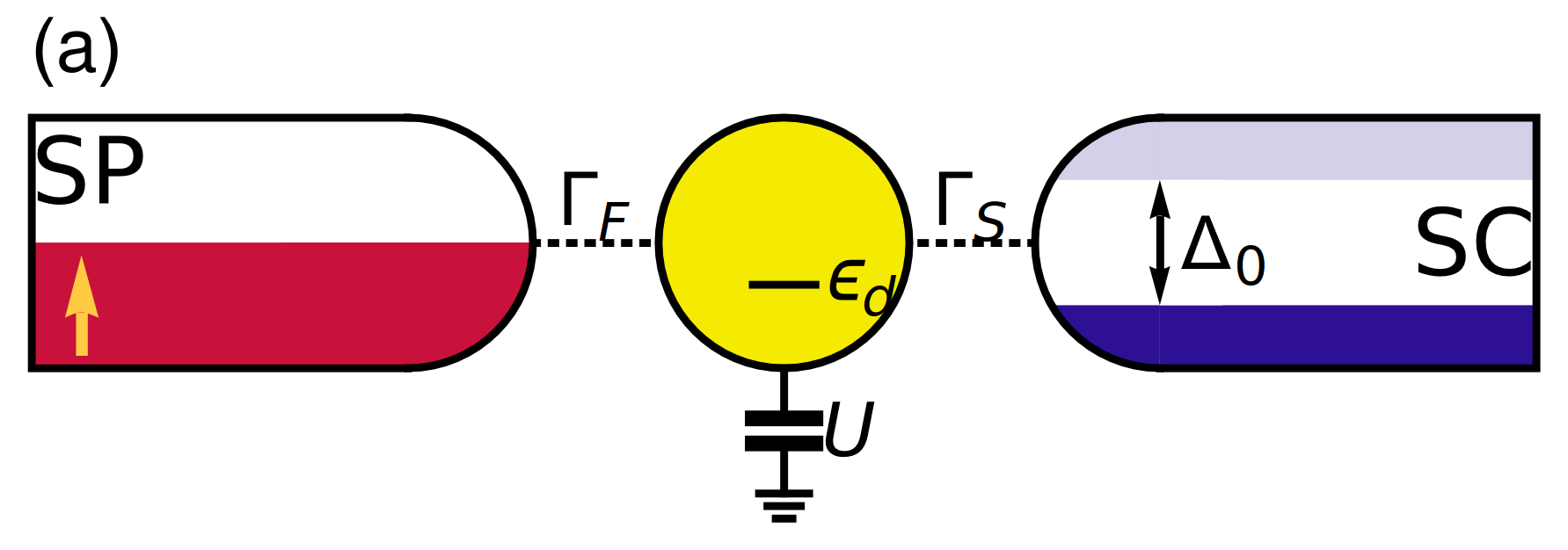
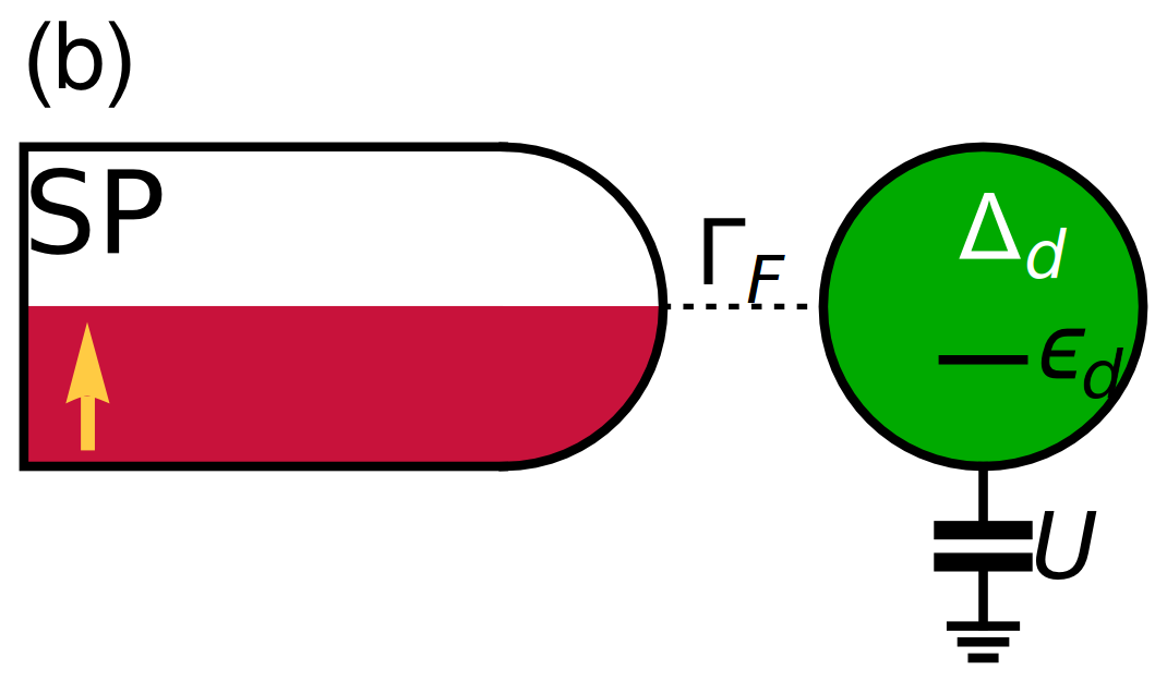
Figure 1: System configurations for (a) the spin-polarized (SP) lead-quantum dot-superconducting (SC) lead and (b) the spin-polarized lead-quantum dot with the proximity-induced superconductivity. Refer the definition of the symbols to the text.

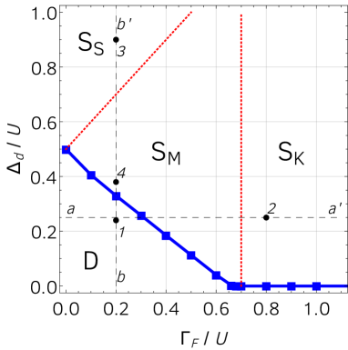
Figure 2: (color online) Phase diagram obtained from the NRG method. The phase boundary (thick solid line) divides the spin singlet (S) and doublet (D) phases. The crossover boundaries (red dotted lines) further divide the singlet phase into the superconductivity-dominant (S_S), mixed-valence (S_M), and Kondo (S_K) singlet regimes, which are connected adiabatically. The black dashed lines are the guides along which we examine the change of physical properties of the system.

We find that unlike the aforementioned pairwise competition among the three effects, the triad interplay is “cooperative” in certain sense and leads to a new quantum phase transition between doublet and singlet states; see Fig. 2. The singlet phase is in many respects similar to the mixed-valence state, but connected adiabatically (through crossovers) to the superconducting state in the limit of strong coupling to the superconductor and to the ‘charge Kondo state’ in the limit of strong coupling to the spin-polarized electrode. The results are obtained with the numerical renormalization group (NRG) method, and the physical explanations are supplemented by other analytic methods such as scaling theory, variational method, and bosonization. Based on the analysis of the characteristics of the phases, we propose three experimental methods to identify the phases, which measure the dot density of state, the cross-current correlation, and the current response to a small ac gate voltage (charge relaxation resistance), respectively.

The rest of the paper is organized as following: We describe explicitly our system and the equivalent models for it in Section II. We report our results based on the NRG method, the quantum phase diagram of the system and the characteristic properties of the phases and crossover regions in the singlet phase in Section III. In Section IV, we apply several analytic methods to provide physical interpretations of the quantum phase transition and the characteristic properties of the different phases and crossover regions. In Section V, we discuss possible experiments to observe our findings. Section VI summarizes the work and concludes the paper.

II Model

Figure 1 (a) shows the schematic configuration of the system of our interest, in which an interacting quantum dot is coupled to both a ferromagnetic lead and a superconducting lead. To stress our points, we consider the extreme case where the ferromagnetic lead is fully polarized end (a) and the superconductivity is very strong (the superconducting gap is the largest energy scale). Recall that with the QD coupled to either a fully polarized ferromagnet or a strong superconductor (but not both), neither charge nor spin fluctuations are allowed on the QD.

First highlighting the fully polarized ferromagnetic lead, the Hamiltonian of the system is written as

$$H=H_{\mathrm{QD}}+H_{\mathrm{F}}+H_{\mathrm{S}}+H_{\mathrm{T}}$$ (1)

with

$$H_{\mathrm{QD}} =\delta\sum_{\mu}(n_{\mu}-1/2)+U(n_{\uparrow}-1/2)(n_{\downarrow}-1/2)$$ (2a)

$$H_{\mathrm{F}} =\sum_{k}\epsilon_{k}c_{k\uparrow}^{\dagger}c_{k\uparrow}$$ (2b)

$$H_{\mathrm{S}} =\sum_{k\mu}\varepsilon_{k}a_{k\mu}^{\dagger}a_{k\mu}-\sum_{k}(\Delta_{0}a_{k\uparrow}^{\dagger}a_{-k\downarrow}^{\dagger}+(h.c.))$$ (2c)

$$H_{\mathrm{T}} =\sum_{k}(t_{F}d_{\uparrow}^{\dagger}c_{k\uparrow}+h.c.)+\sum_{k\mu}(t_{S}d_{\mu}^{\dagger}a_{k\mu}+h.c.).$$ (2d)

The operator $d_{\mu}^{\dagger}$ creates an electron with energy $\epsilon_{d}$ and spin $\mu=\uparrow,\downarrow$ and defines the number operator $n_{\mu}:=d_{\mu}^{\dagger}d_{\mu}$; $n_{d}:=\sum_{\mu}n_{\mu}$. The dot electrons interact with each other with the strength $U$. As mentioned above, the ferromagnetic lead Hamiltonian $H_{F}$ involves only the majority spin ($\uparrow$) electrons, which are described by the fermion operator $c_{k\uparrow}$ with momentum $k$ and energy $\epsilon_{k}$. In the superconducting lead, the operator $a_{k\mu}$ describes the electron with momenum $k$, spin $\mu$, and single-particle energy $\varepsilon_{k}$, and the terms in the pairing potential $\Delta_{0}$ are responsible for the Cooper pairs. Since the superconducting phase is irrelevant in this study, $\Delta_{0}$ is assumed to be real and positive. The tunnelings between the dot and the ferromagnetic/superconducting leads are denoted by $t_{F/S}$, respectively, which are assumed to be momentum-independent for simplicity. The tunnelings induce the hybridizations $\Gamma_{S/F}:=\pi\rho_{S/F}|t_{S/F}|^{2}$ between the dot and the superconducting/ferromagnetic leads, respectively, where $\rho_{S/F}$ are the density of states at the Fermi level in the leads.

The parameter $\delta:=\epsilon_{d}+U/2$ indicates the deviation from the particle-hole symmetry. To make our points clearer and simplify the discussion, in this work we focus on the particle-hole symmetric case $(\delta=0)$. While the particle-hole asymmetry gives rise to some additional interesting features end (b), the underlying physics can be understood in terms of that in the symmetric case.

Next we exploit the strong superconductivity to further simplify our model: The pairing gap of the superconducting lead dominates over the other energy scales ($\Delta_{0}\gg U,\Gamma_{S},\Gamma_{F}$) including $\Delta_{0}\gg T_{K}^{0}$, where $T_{K}^{0}$ is the Kondo temperature in the absence of ferromagnetic lead $(t_{F}=0)$ and the superconductivity $(\Delta_{0}=0)$. In such a limit, the role of the superconducting lead is completely manifested in the proximity induced pairing potential on the QD. Hence, as far as the physics below the superconducting gap is concerned, the effective low-energy Hamiltonian [see Fig. 1 (b)] can be approximated, by integrating out the superconducting degrees of freedom, as

$$H=H_{\mathrm{SQD}}+H_{\mathrm{F}}+H_{\mathrm{T}}$$ (3)

with

$$H_{\mathrm{SQD}} =U\left(n_{\uparrow}-\frac{1}{2}\right)\left(n_{\downarrow}-\frac{1}{2}\right)+\Delta_{d}(d_{\uparrow}^{\dagger}d_{\downarrow}^{\dagger}+d_{\downarrow}d_{\uparrow}),$$ (4a)

$$H_{\mathrm{F}} =\sum_{k}\epsilon_{k}c_{k\uparrow}^{\dagger}c_{k\uparrow}\,,$$ (4b)

$$H_{\mathrm{T}} =\sqrt{\frac{\Gamma_{F}}{\pi\rho_{F}}}\sum_{k}(d_{\uparrow}^{\dagger}c_{k\uparrow}+c_{k\uparrow}^{\dagger}d_{\uparrow})\,,$$ (4c)

where the proximity-induced superconducting gap is given by $\Delta_{d}\sim\Gamma_{S}$ Volkov et al. (1995); McMillan (1968). In this work, we focus on Eq. (3) unless specified otherwise.

In passing, the isolated QD with pairing potential (4a) is diagonalized with the eigenstates and the corresponding energies:

$$\mathinner{\lvert{\textstyle D_{\mu}^{0}}\rangle} =d_{\mu}^{\dagger}\mathinner{\lvert{\textstyle 0}\rangle}, E_{D}^{0} =-U/4\,,\quad(\mu=\uparrow,\downarrow)$$ (5a)

$$\mathinner{\lvert{\textstyle S_{\pm}^{0}}\rangle} =\frac{1\pm d_{\uparrow}^{\dagger}d_{\downarrow}^{\dagger}}{\sqrt{2}}\mathinner{\lvert{\textstyle 0}\rangle}, E_{S\pm}^{0} =U/4\pm\Delta_{d}$$ (5b)

The unperturbed ground state of the QD experiences a transition from the spin doublet state $\mathinner{\lvert{\textstyle D_{\mu}^{0}}\rangle}$ to the spin singlet state $\mathinner{\lvert{\textstyle S_{-}^{0}}\rangle}$ at $\Delta_{d}/U=1/2$.

II.1 Relation to Other Models

Upon the Bogoliubov-de Gennes (BdG) transformation

$$\begin{bmatrix}d_{\uparrow}\\ d_{\downarrow}^{\dagger}\end{bmatrix}=\frac{1}{\sqrt{2}}\begin{bmatrix}1&+1\\ 1&-1\end{bmatrix}\begin{bmatrix}f_{\Uparrow}\\ f_{\Downarrow}^{\dagger}\end{bmatrix},$$ (6)

the Hamiltonian (3) is rewritten as

$$H=\epsilon_{f}\sum_{\sigma=\Uparrow,\Downarrow}f_{\sigma}^{\dagger}f_{\sigma}+Uf_{\Uparrow}^{\dagger}f_{\Uparrow}f_{\Downarrow}^{\dagger}f_{\Downarrow}+\sum_{k}\epsilon_{k}c_{k\uparrow}^{\dagger}c_{k\uparrow}\\ {}+\sqrt{\frac{\Gamma_{F}}{2\pi\rho_{F}}}\sum_{k}\left[c_{k\uparrow}^{\dagger}\left(f_{\Uparrow}+f_{\Downarrow}^{\dagger}\right)+h.c.\right]$$ (7)

with $\epsilon_{f}=\Delta_{d}-U/2$. The Hamiltonian in Eq. (7) describes a single-orbital Anderson-type impurity level $\epsilon_{f}$ with onsite interaction $U$, coupled to a spin-polarized conduction band with strength $\Gamma_{F}/2$. Despite the formal similarity, there are two important distinction between the model (7) and the conventional single-impurity Anderson model: (i) The model (7) involves the pair tunneling, $c_{k\uparrow}^{\dagger}f_{\Downarrow}^{\dagger}$, which will turn out to play a crucial role below. (ii) The spin index $\sigma=\Uparrow,\Downarrow$ for $f_{\sigma}$ indicates the spin direction along the spin $x$-direction whereas $\mu=\uparrow,\downarrow$ for $d_{\mu}$ along the spin $z$-direction.

On the other hand, the particle-hole transformation

$$d_{1}=d_{\uparrow},\quad d_{2}=d_{\downarrow}^{\dagger},$$ (8)

transforms the model (3) to

$$H=-U(n_{1}-1/2)(n_{2}-1/2)+\Delta_{d}(d_{1}^{\dagger}d_{2}+d_{2}^{\dagger}d_{1})\\ {}+\sum_{k}\epsilon_{k}c_{k\uparrow}^{\dagger}c_{k\downarrow}+\sqrt{\frac{\Gamma_{F}}{\pi\rho_{F}}}\sum_{k}(d_{1}^{\dagger}c_{k\uparrow}+c_{k\uparrow}^{\dagger}d_{1})\,.$$ (9)

In this model, the ferromagnetic lead is coupled to $d_{1}$ via a normal tunneling and the pairing term has been transformed to a tunneling term between dot orbital levels. It is known as the resonant two-level system with attractive interaction ($-U<0$) Žitko and Pruschke (2009); Žitko and Simon (2011).

II.2 Methods and Physical Quantities

For a non-perturbative study of the many-body effects, we adopt the well-established numerical renormalization group (NRG) method, which provides not only qualitatively but also quantitatively accurate results for quantum impurity systems. Specifically, we exploit the NRG method to identify the different phases of the system as well as to investigate their quantum transport properties. Technically, we impose additional improvements, the generalized Logarithmic discretization Campo and Oliveira (2005); Žitko and Pruschke (2009) with the discretization parameter $\Lambda=2$ and the $z$-averaging Yoshida et al. (1990) with $N_{z}=32$, on the otherwise standard NRG procedure Wilson (1975a); Krishna-murthy et al. (1980a); Bulla et al. (2008). We use the conduction band half-width $D=1$ as the unit of energy.

To identify the phases, we follow the (non-perturbative) renormalization group idea Wilson (1975b); Krishna-murthy et al. (1980a, b) and examine the conserved quantity

$$N_{S}=n_{\uparrow}-n_{\downarrow}+\sum_{k}c_{k\uparrow}^{\dagger}c_{k\uparrow}-N_{0}$$ (10)

of the ground state, where $N_{0}$ is the total charge number of the unperturbed spin-polarized lead at zero temperature. Physically, $N_{S}$ is the excess spin number in the whole system.

The quantum transport properties of different phases and crossover regions are investigated by calculating the local spectral density and the charge relaxation resistance with the NRG method. The local spectral density (or local tunneling density of states) of the QD,

$$A_{\mu}(\omega)=-\frac{1}{\pi\hbar}\mathrm{Im}[G_{\mu}^{R}(\omega)]\,,$$ (11)

is related to the Fourier transform $G_{\mu}^{R}(\omega)$ of the retarded Green’s function $G_{\mu}(t)$ for spin $\mu$, $G_{\mu}(t)=-i\hbar\Theta(t)\mathinner{\left\langle{\{d_{\mu}(t),d_{\mu}^{\dagger}(0)\}}\right\rangle}$. The charge relaxation resistance $R_{q}(\omega)$ describes the response of the displacement current $I(t)$ through the QD in the presence of the ac gate voltage Büttiker et al. (1993a, b); Lee et al. (2011); Lee and Choi (2014). More explicitly, it is defined through the admittance $g(t)=(ie/\hbar)\Theta(t)\mathinner{\left\langle{[I(t),n_{d}(t)]}\right\rangle}$ by the relation $1/g(\omega)=R_{q}(\omega)+i/\omega C_{q}(\omega)$, where $C_{q}(\omega)$ is the quantum correction to the capacitance. The admittance in turn can be extracted from its relation, $g(\omega)=i\omega(e^{2}/\hbar)\chi_{c}(\omega)$ to the dot charge susceptibility $\chi_{c}(t)=-i\Theta(t)\mathinner{\left\langle{[n_{d}(t),n_{d}]}\right\rangle}$, which is directly calculated with the NRG method.

III Results

Figure 2 shows the phase diagram which exhibits a quantum phase transition between two phases, the spin singlet (S) and doublet (D) phases, identified by the quantum number $N_{S}$ of the ground state calculated with the NRG method. Across the phase boundary, the quantum number $N_{S}$ of the ground state changes from $N_{S}=\pm 1$ (doublet) to $N_{S}=0$ (singlet). In addition, apart from the phase transition, we have found two crossovers further distinguishing three regimes inside the singlet phase: superconductivity-dominant ($\mathrm{S_{S}}$), mixed-valence (S_M), and Kondo (S_K) singlet regimes. Below, we detail some interesting characteristics of each phase.

III.1 Double Phase

The doublet phase occupies the region of smaller $\Delta_{d}$ and $\Gamma_{F}$ of the phase diagram in Fig. 2. The phase boundary is roughly linear for $\Gamma_{F}/U\ll 1/2$ as described by the equation

$$\Delta_{d}/U+\Gamma_{F}/U\approx 1/2\,.$$ (12)

Note that the ground state remains doubly degenerate with the excess spin number $N_{S}=\pm 1$ even in the presence of the coupling to the spin-polarized ferromagnetic lead. It is due to the particle-hole symmetry. With the particle-hole symmetry is broken, the degeneracy is lifted at finite $\Gamma_{F}$ and the phase boundary is shifted accordingly end (b).

In the doublet phase, the local spectral densities $A_{\mu}(\omega)$ on the QD exhibit typical charge-fluctuation peaks at $|\hbar\omega|\sim E_{S\pm}^{0}-E_{D}^{0}=U/2\pm\Delta_{d};$ see Figs. 3 (a) and (b). Apart from those charge-fluctuation peaks, $A_{\downarrow}(\omega)$ has an additional power-law peak at the zero frequency $\omega=0$, $A_{\downarrow}(\omega)\propto|\omega|^{-\alpha}$ [see Fig. 3 (b)]. This power-law peak at the zero energy suggests that the doublet phase is ‘marginal’ in the RG sense. The exponent $\alpha$ is found to increase monotonically with increasing $\Gamma_{F}$ and $\Delta_{d}$, and is well fitted to $\alpha=1-(2/\pi)\tan^{-1}(U/2\Gamma_{F})$ for small $\Delta_{d}$ [see Fig. 3 (c)].

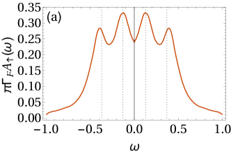
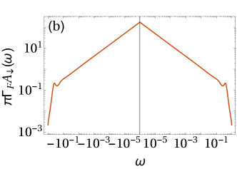
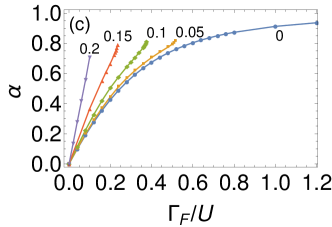
Figure 3: (a,b) Spin-dependent spectral densities $A_{\mu}(\omega)$ in the spin doublet phase, corresponding to the point $1$ in Fig. 2. Here we have used $U=0.5D$, $\Gamma_{F}=0.1D$, and $\Delta_{d}=0.12D$. The dotted lines in (a) indicate the frequencies $|\hbar\omega|=U/2\pm\Delta_{d}$. (c) The exponent $\alpha$ from the power-law relation of $A_{\downarrow}(\omega)$. The line is a fitting curve for $\Delta_{d}=0$; see the text for the expression for it. The value of $\Delta_{d}/D$ are annotated.

III.2 Singlet Phase: Superconductivity-Dominant Singlet

For larger values of $\Delta_{d}$, the system has a singlet ground state. In particular, the region of larger $\Delta_{d}/U$ and smaller $\Gamma_{F}/U$ of the phase diagram Fig. 2 is characterized by the strong Cooper pairing. It is natural as the ground state of the unperturbed QD ($\Gamma_{F}=0$) is the spin singlet $\mathinner{\lvert{\textstyle S_{-}^{0}}\rangle}$ composed of empty or doubly occupied states [see Eq. (5)] due to the proximity-induced superconductivity. Such superconductivity-dominant singlet region is separated from other singlet regions by a crossover boundary, roughly described by the equation [cf. Eq. (12)]

$$\Delta_{d}/U-\Gamma_{F}/U\approx 1/2\,.$$ (13)

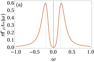
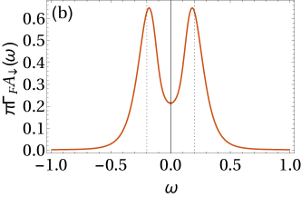
Figure 4: Dot spectral densities in the superconductivity-dominant singlet regime corresponding to the point $3$ in Fig. 2. Here we have used $U=0.5D$, $\Gamma_{F}=0.4D$, and $\Delta_{d}=0.45D$. The dotted lines indicate the frequencies $|\hbar\omega|=\Delta_{d}-U/2$. In (a), the spectral density vanishes at zero frequency due a Fano-like destructive interference.

Because in this regime the superconductivity prevails over all the other types of correlations, the dot spectral densities [see Figs. 4 (a) and (b)] are simply given by the charge fluctuation peaks at $|\hbar\omega|\sim E_{D}^{0}-E_{S-}^{0}=\Delta_{d}-U/2$, broadened by the weak tunnel coupling $\Gamma_{F}$.

However, there is one noticeable feature in the spin-up spectral density $A_{\uparrow}(\omega)$. That is, $A_{\uparrow}(\omega=0)=0$ exactly, which is the consequence of the Fano-like destructive interference between two kinds of dot-lead tunneling processes. It will be discussed in detail in Section IV.3.

III.3 Singlet Phase: Mixed-Valence Singlet

The most interesting singlet phase occurs near $\Delta_{d}/U\approx 1/2$ with finite $\Gamma_{F}/U$ in the phase diagram (Fig. 2). We call it a “mixed-valence singlet” region because $\epsilon_{f}<\Gamma_{f}$ in the model (7) regarding $\epsilon_{f}$ and $U$ as independent parameters; see the further discussions in Section IV.4. It is distinguished from the doublet phase by the true phase boundary (12) and separated from the superconductivity-dominant singlet state by the crossover boundary (13); that is,

$$|\Delta_{d}/U-1/2|\approx\Gamma_{F}/U.$$ (14)

It is also separated from still another singlet state for $\Gamma_{F}/U\gg 1$, which is characterized by the Kondo behaviors (see also Section III.4), by another crossover.

The two spin-dependent spectral densities $A_{\mu}(\omega)$ in the mixed-valence singlet state, as shown in Fig. 5, put stark contrast with each other: While $A_{\downarrow}(\omega)$ for the minority spin features a usual Lorentzian peak of width $\Gamma_{-}$ at the zero frequency, $A_{\uparrow}(\omega)$ for the majority spin has a Lorentzian dip of the same width $\Gamma_{-}$ superimposed on a broader peak structure of width $\Gamma_{+}$. Later [see Section IV.4], we will attribute this dip structure to a destructive interference between two different types of tunneling processes based on an effective non-interacting theory.

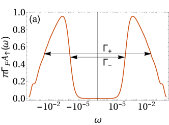
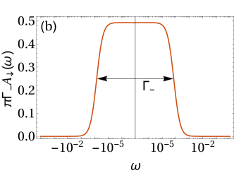
Figure 5: Dot spectral densities in the mixed-valence singlet regime at the point $4$ in Fig. 2. Here we have used $U=0.5D$, $\Gamma_{F}=0.4D$, and $\Delta_{d}=0.19D$.

III.4 Singlet Phase: Kondo Singlet

When the QD couples strongly with the spin-polarized lead ($\Gamma_{F}/U\gg 1,\Delta_{d}/U$), the system displays still another type of singlet correlation. We call this state as a Kondo singlet state as it corresponds to the so-called ‘charge Kondo state’ Matveev (1991); Iftikhar et al. (2015); see Section IV.5. In the charge Kondo state, the excess charge on the QD plays the role of a pseudo-spin.

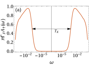
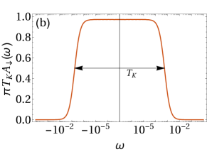
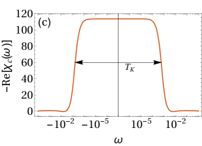
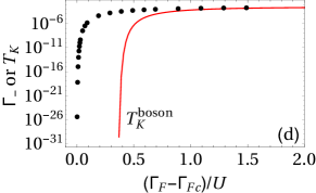
Figure 6: (a,b,c) Dot spectral densities and charge susceptibility in the Kondo regime of the singlet phase at point $2$ in Fig. 2. Here we have used $U=0.5D$, $\Gamma_{F}=0.4D$, and $\Delta_{d}=0.125D$. (d) The width of the central peak of $A_{\downarrow}(\omega)$ and $T_{K}^{\mathrm{boson}}$ from Eq. (29) at $\Delta_{d}=0.125D$.

As shown in Fig. 6, the peak shapes of the spectral densities $A_{\mu}(\omega)$ are similar to those in the mixed-valence singlet state described in Section III.3. The dip structure in $A_{\uparrow}(\omega)$ for the majority spin is again attributed to the Fano-like destructive interference. However, the normalized peak height $\pi T_{K}A_{\downarrow}(\omega)$ for the minority spin is now unity, demonstrating the charge Kondo effect; the peak height of $\pi\Gamma_{-}A_{\downarrow}(\omega=0)$ grows from zero to unity as one moves from the mixed-valence regime to the Kondo regime [compare Fig. 6 (b) with Fig. 5 (b)]. Further, the peak width of $A_{\downarrow}(\omega)$, or the dip width of $A_{\uparrow}(\omega)$, is identified as the charge Kondo temperature $T_{K}$.

The charge Kondo effect is also manifested in the charge susceptibility $\chi_{c}(\omega)$ of the QD shown in Fig. 6 (c). Its real part displays a pronounced central peak of the same width $T_{K}$. In the conventional (spin) Kondo effect, this susceptibility corresponds to the spin susceptibility.

IV Discussion

The NRG calculations reported in the previous section clearly display a quantum phase transition between the spin singlet and doublet phases. Here we use some analytical but approximate methods to understand deeper the nature of the transition and the characteristics of the different phases.

As seen in the equivalent model (7), our system is described by a generalized form of the Anderson impurity model. The Anderson impurity model Anderson (1961) has been studied in various theoretical methods; using the variational method Varma and Yafet (1976), the scaling theory Jefferson (1977); Haldane (1978), the numerical renormalization group method Krishna-murthy et al. (1980b), and the $1/N$ expansion Ramakrishnan and Sur (1982). Here we extend some of these methods.

IV.1 Mixed-Valence Transition

We first examine analytically the phase boundary between the doublet and singlet phases found in Section III based on the NRG method. Our analysis consists of two steps depending on the relevant energy scale. At higher energies (the band cutoff $\Lambda\gtrsim\Gamma_{F}$), we extend the scaling theory Jefferson (1977); Haldane (1978) to integrate out the high-energy excitations. At lower energies ($\Lambda<\Gamma_{F}$), we extend the variational method Varma and Yafet (1976).

Following Haldane’s scaling argument Jefferson (1977); Haldane (1978), it is straightforward to integrate out the high energy states in the conduction band up to $\Gamma_{F}$ and keep track of the scaling of the parameters $\epsilon_{f}$ and $U$ in the equivalent model (7); concerning the model (7) it is convenient to regard $\epsilon_{f}$ and $U$ (rather than $\Delta_{d}$ and $U$) as independent parameters. We found that even though our system has only a single spin channel the anomalous tunneling term acts as the tunneling via the second spin channel so that the scaling result is exactly the same as the one for the conventional Anderson model:

$$\epsilon_{f}(\Lambda)=\epsilon_{f}^{*}-\frac{\Gamma_{F}}{\pi}\ln\frac{\Lambda}{\Gamma_{F}}$$ (15)

with the scaling invariant $\epsilon_{f}^{*}=\epsilon_{f}(\Lambda=\Gamma_{F})$ and the band cutoff $\Lambda$. Therefore, as in the conventional Anderson impurity model, it is possible to identify three regimes: the empty/doubly-occupied ($|\epsilon_{f}^{*}|\gg\Gamma_{F}$), the mixed-valence ($|\epsilon_{f}^{*}|\lesssim\Gamma_{F}$), and the local-moment regimes ($\epsilon_{f}^{*}\ll-\Gamma_{F}$). For the conventional Anderson impurity model, in all these regimes the renormalization beyond the Haldane’s scaling eventually flows into the spin singlet state, so there are only crossovers between the regimes. However, for our system the local-moment regime does not flow into the singlet state because there is only a single spin channel and the anomalous tunneling term prevents the formation of the conventional Kondo correlation. Therefore, a transition takes place between the mixed-valence and local-moment regimes; hence the transition is named as the mixed-valence one.

To see this more clearly, we extend the variational method. Here we focus on the case of $U\to\infty$. This condition rules out the doubly occupied state on the QD (recall that concerning the model (7) $\epsilon_{f}$ and $U$ are regarded as independent parameters) and makes the variational analysis much simpler; the finite $U$ should involve more states but would not alter the main qualitative feature of the transition found in the $U\to\infty$ case. We take a variational ansatz for the ground states in spin singlet and doublet states, respectively, up to the second order in the dot-lead tunneling

$$\mathinner{\lvert{\textstyle S}\rangle} =\left[\alpha_{0}+\sum_{k<k_{F}}\alpha_{k+}f_{\Uparrow}^{\dagger}c_{k\uparrow}+\sum_{k>k_{F}}\alpha_{k-}c_{k\uparrow}^{\dagger}f_{\Downarrow}^{\dagger}+\sum_{k>k_{F},k^{\prime}<k_{F}}\alpha_{kk^{\prime}}c_{k\uparrow}^{\dagger}c_{k^{\prime}\uparrow}\right]\mathinner{\lvert{\textstyle\mathrm{FS}}\rangle}_{0}$$ (16a)

$$\mathinner{\lvert{\textstyle D_{\uparrow}}\rangle} =\left[\beta_{0}f_{\Uparrow}^{\dagger}+\sum_{k>k_{F}}\beta_{k}c_{k\uparrow}^{\dagger}+\sum_{k>k_{F},k^{\prime}<k_{F}}\left(\beta_{kk^{\prime}+}f_{\Uparrow}^{\dagger}c_{k\uparrow}^{\dagger}c_{k^{\prime}\uparrow}+\beta_{kk^{\prime}-}c_{k\uparrow}^{\dagger}c_{k^{\prime}\uparrow}^{\dagger}f_{\Downarrow}^{\dagger}\right)\right]\mathinner{\lvert{\textstyle\mathrm{FS}}\rangle}_{0},$$ (16b)

where $\mathinner{\lvert{\textstyle\mathrm{FS}}\rangle}_{0}$ is unperturbed Fermi sea and $k_{F}$ is the Fermi wave number. The states satisfy the normalization condition, $\mathinner{\left\langle{S|S}\right\rangle}=\mathinner{\left\langle{D_{\uparrow}|D_{\uparrow}}\right\rangle}=1$. The coefficients $\alpha$ and $\beta$ in these two states are to be determined by the minimization condition of the energy expectation value with respect to these states: $\mathinner{\left\langle{S|H|S}\right\rangle}:=E_{0}+\epsilon_{f}+\epsilon_{S}$ and $\mathinner{\left\langle{D_{\uparrow}|H|D_{\uparrow}}\right\rangle}:=E_{0}+\epsilon_{f}+\epsilon_{D}$, where $E_{0}$ is the unperturbed energy of $\mathinner{\lvert{\textstyle\mathrm{FS}}\rangle}_{0}$. By applying the Lagrange multiplier method under the normalization constraint, we obtain the coupled differential equations:

$$\epsilon_{S}\alpha_{0} =-\epsilon_{f}\alpha_{0}+\frac{t_{F}}{\sqrt{2}}\left(\sum_{k<k_{F}}\alpha_{k+}-\sum_{k>k_{F}}\alpha_{k-}\right)$$ (17a)

$$\epsilon_{S}\alpha_{k+} =\frac{t_{F}}{\sqrt{2}}\alpha_{0}-\epsilon_{k}\alpha_{k+}+\frac{t_{F}}{\sqrt{2}}\sum_{k^{\prime}>k_{F}}\alpha_{k^{\prime}k}$$ (17b)

$$\epsilon_{S}\alpha_{k-} =-\frac{t_{F}}{\sqrt{2}}\alpha_{0}+\epsilon_{k}\alpha_{k-}+\frac{t_{F}}{\sqrt{2}}\sum_{k^{\prime}<k_{F}}\alpha_{kk^{\prime}}$$ (17c)

$$\epsilon_{S}\alpha_{kk^{\prime}} =\frac{t_{F}}{\sqrt{2}}\left(\alpha_{k^{\prime}+}+\alpha_{k-}\right)+(\epsilon_{k}-\epsilon_{k^{\prime}}-\epsilon_{f})\alpha_{kk^{\prime}}$$ (17d)

and

$$\epsilon_{D}\beta_{0} =\frac{t_{F}}{\sqrt{2}}\sum_{k>k_{F}}\beta_{k}$$ (18a)

$$\epsilon_{D}\beta_{k} =\frac{t_{F}}{\sqrt{2}}\beta_{0}+(\epsilon_{k}-\epsilon_{f})\beta_{k}+\frac{t_{F}}{\sqrt{2}}\left[\sum_{k^{\prime}<k}\beta_{k^{\prime}k-}-\sum_{k^{\prime}>k}\beta_{kk^{\prime}-}-\sum_{k^{\prime}<k_{F}}\beta_{kk^{\prime}+}\right]$$ (18b)

$$\epsilon_{D}\beta_{kk^{\prime}+} =-\frac{t_{F}}{\sqrt{2}}\beta_{k}+(\epsilon_{k}-\epsilon_{k^{\prime}})\beta_{kk^{\prime}+}$$ (18c)

$$\epsilon_{D}\beta_{kk^{\prime}-} =-\frac{t_{F}}{\sqrt{2}}(\beta_{k}-\beta_{k^{\prime}})+(\epsilon_{k}+\epsilon_{k^{\prime}})\beta_{kk^{\prime}-}.$$ (18d)

Up to the first order (by setting $\alpha_{kk^{\prime}}=\beta_{kk^{\prime}\pm}=0$), the equations for $\epsilon_{S}$ and $\epsilon_{D}$ can be obtained in closed form:

$$\epsilon_{S} =-\epsilon_{f}-\frac{\Gamma_{F}}{\pi}\ln\left(1+\frac{D}{|\epsilon_{S}|}\right)$$ (19a)

$$\epsilon_{D} =-\frac{\Gamma_{F}}{2\pi}\ln\left(1+\frac{D}{|\epsilon_{D}|-\epsilon_{f}}\right).$$ (19b)

These equations can be solved numerically, and two different phases, in each of which either $\epsilon_{S}<\epsilon_{D}$ or $\epsilon_{S}>\epsilon_{D}$, are identified, as shown in Fig. 7 (a). Although a closed form equations for $\epsilon_{S}$ and $\epsilon_{D}$ are not available with the second-order terms included, the whole differential equation can be solved numerically by discretizing the lead dispersion. It is found that the inclusion of the second-order terms hardly changes the phase boundary. On similar reasoning, one can see that the phase boundary remains intact upon including the higher-order terms in the variational wave functions.

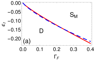
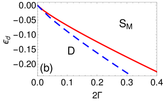
Figure 7: Phase diagrams obtained from the variational method in the $U\to\infty$ limit (a) for our model and (b) for conventional single-impurity Anderson model. The solid and dotted lines are phase boundaries when up to the first and second-order terms are taken into account, respectively.

It is in stark contrast with the similar variational analysis for the conventional Anderson impurity model in Appendix A: Up to the first-order the equations for $\epsilon_{S}$ and $\epsilon_{D}$ are the same as those for our models [see Eq. (34)]. Therefore, at this order a phase transition between the spin singlet and doublet states also takes place even in the conventional Anderson impurity model. This apparent contradiction to the well-known fact that the ground state of the conventional Anderson impurity model is always spin singlet is due to the perturbative construction of the ansatz. As illustrated in Fig. 7 (b), the spin doublet region shrinks for the conventional Anderson model when one includes the higher-order terms. In other words, the Kondo ground state involves all the higher-order singlet states between the dot and the lead Gunnarsson and Schönhammer (1983).

This difference can be inferred from the comparison between two ansatz, Eqs. (16) and (31). For the spin singlet state, the number of the particle-hole excitations in the second-order term for our model is by half smaller than that for the conventional Anderson impurity model because of the difference in the channel numbers. On the other hand, it is not the case for the doublet state. It explains why the singlet state in our model does not lower its energy upon including the higher-order terms, compared to the doublet state, and also why the Kondo correlation cannot arise.

IV.2 Doublet Phase

We now investigate the characteristics of the different phases (and subregions inside the singlet phase). We start with the doublet phase by applying the Schrieffer-Wolff transformation on the assumption that $\Gamma_{F}\ll|\epsilon_{f}|,U$. The model (7) is then transformed to an effective Kondo-like model:

$$H\approx H_{\mathrm{eff}}=J{\mathbf{s}}\cdot{\mathbf{S}}+\sum_{k}\epsilon_{k}c_{k\uparrow}^{\dagger}c_{k\uparrow}\,.$$ (20)

Here the impurity spin-1/2 operator ${\mathbf{S}}$ is defined by

$$S^{+}=(S^{-})^{\dagger}=\mathinner{\lvert{\textstyle\Uparrow}\rangle}\mathinner{\langle{\textstyle\Downarrow}\rvert}\,,\quad S^{z}=\mathinner{\lvert{\textstyle\Uparrow}\rangle}\mathinner{\langle{\textstyle\Uparrow}\rvert}-\mathinner{\lvert{\textstyle\Downarrow}\rangle}\mathinner{\langle{\textstyle\Downarrow}\rvert}\,,$$ (21)

where

$$\mathinner{\lvert{\textstyle\sigma}\rangle}=f_{\sigma}^{\dagger}\mathinner{\lvert{\textstyle 0}\rangle}\quad(\sigma=\Uparrow,\Downarrow)\,.$$ (22)

On the other hand, the conduction-band spin, ${\mathbf{s}}=\sum_{kk^{\prime}\nu\nu^{\prime}}\psi_{k\nu}^{\dagger}{\boldsymbol{\tau}}_{\nu\nu^{\prime}}\psi_{k^{\prime}\nu^{\prime}}$ is defined over the two-component Nambu spinor $\psi_{k\nu}$ with $\psi_{k1}=c_{k\uparrow}$ and $\psi_{k2}=c_{k\uparrow}^{\dagger}$ with ${\boldsymbol{\tau}}$ being the Pauli matrices in the Nambu space (i.e. the particle-hole isospin space). The isotropic exchange coupling is obtained as $\rho_{F}J\approx\Gamma_{F}/\pi|\epsilon_{f}|$. The model (20) is formally the same as the usual Kondo model except the fact that the conduction spin is replaced by the isospin in the Nambu space. This replacement, however, makes a crucial difference in poor man’s scaling Anderson (1970); Krishna-murthy et al. (1980a, b). For example, the typical scaling of $J_{z}$ term vanishes at least up to the second order:

$$-2\frac{J_{\perp}^{2}}{\epsilon_{k_{3}}}\left(c_{k_{1}}\dot{c}_{k_{2}}\dot{c}_{k_{3}}^{\dagger}c_{k_{4}}^{\dagger}+\dot{c}_{k_{2}}c_{k_{1}}\dot{c}_{k_{3}}^{\dagger}c_{k_{4}}^{\dagger}\right)\mathinner{\lvert{\textstyle\uparrow}\rangle}\mathinner{\langle{\textstyle\uparrow}\rvert}\approx 0\,.$$ (23)

These results imply that unlike the true Kondo model involving real spins, the exchange coupling in Eq. (20) involving particle-hole isospins is marginal in the RG sense. Namely, it does not scale as one goes down to lower energies. The NRG results discussed in Section III.1 support this scaling analysis.

IV.3 Singlet Phase: Superconductivity-Dominant Singlet

The superconductivity-dominant singlet phase can be easily understood within the perturbative argument. When the QD is isolated ($\Gamma_{F}=0$), the pairing potential $\Delta_{d}$ dominates over the on-site interaction $U$ for $\Delta_{d}/U>1/2$; see Eq. (5). As the tunneling coupling $\Gamma_{F}$ is turned on, the above feature does not change qualitatively unless $\Gamma_{F}$ exceeds $\Delta_{d}$ significantly. As $\Gamma_{F}/U$ grows further beyond $\Delta_{d}/U-1/2$, the state gradually crosses over to the mixed-valence singlet state.

IV.4 Singlet Phase: Mixed-Valence Singlet

The mixed-valence singlet phase, $|\Delta_{d}/U-1/2|\lesssim\Gamma_{F}/U\lesssim 1$, is roughly similar to the mixed-valence regime of the conventional Anderson impurity model. Recall that in the equivalent model (7), the impurity energy level is given by $\epsilon_{f}=\Delta_{d}-U/2$ and according to the above phase boundary, $\epsilon_{f}<\Gamma_{F}$, and hence the name mixed-valence singlet state.

The most noticeable feature of the mixed-valence singlet region is the emergence of the two energy scales $\Gamma_{\pm}$ in the local spectral densities, as demonstrated in Fig. 5. To understand it, we first note that in this phase ($\Gamma_{F}>\epsilon_{f}$) the charge fluctuation on the QD is huge and at the zeroth order the effects of the on-site interaction $U$ may be ignored. In the non-interacting picture, the dot Green’s functions given by

$$G_{\uparrow}^{R}(\omega) =\frac{1}{\Gamma_{+}-\Gamma_{-}}\left[\frac{\Gamma_{+}}{\omega+i\Gamma_{+}}-\frac{\Gamma_{-}}{\omega+i\Gamma_{-}}\right],$$ (24a)

$$G_{\downarrow}^{R}(\omega) =\frac{1}{\Gamma_{+}-\Gamma_{-}}\left[\frac{\Gamma_{+}}{\omega+i\Gamma_{-}}-\frac{\Gamma_{-}}{\omega+i\Gamma_{+}}\right],$$ (24b)

clearly exhibits two energy scales

$$\Gamma_{\pm}=\Gamma_{F}/2\pm\sqrt{(\Gamma_{F}/2)^{2}-\epsilon_{f}^{2}}\,,$$ (25)

which represent the relaxation rates predominantly via the normal tunneling ($c_{k\uparrow}^{\dagger}f_{\Uparrow}$) and the pair tunneling ($c_{k\uparrow}^{\dagger}f_{\Downarrow}^{\dagger}$), respectively. The normal- and pair-tunneling processes are accompanied by phase shift $\pi$ relative to each other and lead to destructive interference; recall $d_{\uparrow}=(f_{\Uparrow}+f_{\Downarrow}^{\dagger})/\sqrt{2}$ from the transformation (6). The destructive interference is maximal at zero frequency so that $A_{\uparrow}(\omega)$ has a dip with a width $\Gamma_{-}$ inside the central peak whose width is $\Gamma_{+}$. For spin $\downarrow$, two processes simply add up so that two peaks are superposed, displaying a very sharp peak of the width $\Gamma_{-}$.

While the non-interacting theory explains the feature of the spectral densities qualitatively, the NRG results in Section III.3 uncover that the interaction $U$ significantly renormalizes $\epsilon_{f}$ and hence $\Gamma_{\pm}$ such that $\Gamma_{-}\ll\Gamma_{+}\ll\Gamma_{F}$. Especially, $\Gamma_{-}$ decreases exponentially with decreasing $\Gamma_{F}$ and vanishes at the transition point. One way to investigate such renormalization effects is again to use the extended variational method in Section IV.1 including all orders Varma and Yafet (1976); Gunnarsson and Schönhammer (1983). It is, however, out of the scope of the present work and leave it open for future studies.

IV.5 Singlet Phase: Kondo Singlet

Now we turn to the Kondo singlet regime with $\Gamma_{F}/U\gg 1,\Delta_{d}/U$. In Section II.1 we have seen that our model, (3) or (7), is equivalent to the resonant two-level model with negative interaction, (9). In a recent work Žitko and Simon (2011) along a different context, it has been found that the resonant two-level model in the large $\Gamma_{F}$ limit can be bosonized and thus mapped to the anisotropic Kondo model. Interestingly, it was also shown to be related to a quantum impurity coupled to helical Majorana edge modes formed around a two-dimensional topological superconductor. Here we adopt their result to our context, referring the details of the derivation to Ref. Žitko and Simon (2011).

Following the bosonization procedure Žitko and Simon (2011), the interacting resonant two-level model is mapped to a bosonized form of the anisotropic Kondo model

$$H_{K}=\sum_{k\sigma}\epsilon_{k}c_{k\sigma}^{\dagger}c_{k\sigma}+\frac{J_{\perp}}{2}(S^{+}s^{-}+S^{-}s^{+})+J_{z}S^{z}s^{z}$$ (26)

with the conduction-band spin ${\mathbf{s}}$ and the impurity spin ${\mathbf{S}}$. Here the Kondo couplings are identified as

$$J_{\perp}=\sqrt{8}\Delta_{d}$$ (27)

and

$$\sqrt{2}\left[1-\frac{2}{\pi}\tan^{-1}\frac{\pi\rho J_{z}}{4}\right]=\gamma:=1+\frac{2}{\pi}\tan^{-1}\frac{U}{\Gamma_{F}}.$$ (28)

For sufficiently large $\Gamma_{F}$ compared to $U$, this Kondo model is antiferromagnetic $(J_{\perp},J_{z}>0)$, and the effective Kondo temperature associated with the screening of the magnetic moment is, from the known results on the Kondo model,

$$T_{K}^{\mathrm{boson}}\sim\frac{\Gamma_{F}}{2}\left(\frac{2\Delta_{d}}{\Gamma_{F}}\right)^{\frac{2}{2-\gamma^{2}}}.$$ (29)

As clear from the bosonization procedure, the anisotropic Kondo model essentially corresponds to the so-called ‘charge Kondo effect’ with the excess charge on the QD playing the role of the pseudo-spin Matveev (1991); Iftikhar et al. (2015). More specifically, the charging of $d_{\downarrow}$ level is mapped onto the pseudo-spin of the Kondo impurity. Considering that the ferromagnetic lead in our original model has only a single spin component, this Kondo model should be defined in particle-hole isospin space of both the dot and the lead. Then, the spin-flip scattering in the effective Kondo model can be interpreted as the particle-hole scattering in our original model. For example, the injected particle in the lead is scattered into the hole, accompanying the inversion of the occupation of $d_{\downarrow}$ level. Since the change in the occupation of $d_{\downarrow}$ level is only possible via the pair tunneling to the superconducting lead, the Kondo correlation implies that the currents in the ferromagnetic and superconducting leads are highly correlated.

Here it should be noted that the interpretation based on the bosonization is valid only in the large-$\Gamma_{F}$ limit because the bosonization procedure requires the unbounded momentum (or dispersion) of a continuum band (whose band width is $\Gamma_{F}$ in our case) which is to be bosonized. Hence, the mapping to the anisotropic Kondo model cannot be justified in general; in this respect our parameter regime and interpretation are different from those of Ref. Žitko and Simon (2011), where the singlet and doublet phases and the phase transition between them are explained in terms of the effective Kondo model. One evidence supporting the limitation of the bosonization may come from the comparison between the width of the central peak of $A_{\downarrow}(\omega)$, which is $T_{K}$ in the S_K regime, and the effective Kondo temperature, Eq. (29), predicted from the bosonization [see Fig. 6 (d)]. Two energy scales are in good agreement with each other for $\Gamma_{F}/U>1$, as expected. However, for $\Gamma_{F}/U\lesssim 1$, there is a big discrepancy between them. In addition, the expression (29) fails close to the transition point. It indicates that the region of the singlet phase with small $\Gamma_{F}$ is not of the Kondo state but of the mixed-valence state, as discussed in the previous section.

V Possible Experiments

Up to now, we have elucidated the physical nature of the two phases and, in particular, classified the different regimes in the singlet phase, mostly based on the dot spectral densities. One remaining question is how to make a distinction between the different regimes in experiment. Here we suggest three possible experimental observations: the spin-selective tunneling microscopy, the current correlation between leads, and the the dynamical response with respect to the ac gate voltage.

The characteristics of different phases and regimes are well reflected in the spin-dependent spectral density which can be measured by the spin-selective tunneling microscopy applied directly to the quantum dot. It corresponds to adding of an additional ferromagnetic lead very weakly connected to the quantum dot and measuring the differential conductance through it. By altering the polarization of the auxiliary ferromagnetic lead, one can measure the spectral density of the quantum dot for each spin, identifying different phases based on it.

Secondly, as explained in Sec. IV.5, the Kondo scattering in the S_K regime correlates the currents in the ferromagnetic and superconducting leads, resulting in nontrivial cross-current correlation which can be measured in experiment. Obviously, the average current from the fully polarized ferromagnetic lead to the superconducting lead is still zero in the presence of interacting quantum dot because there is no influx of spin-$\downarrow$ electron from the ferromagnetic lead. However, different from previous works on similar systems de Jong and Beenakker (1995); Cao et al. (2004), the strong interaction in our system makes the currents correlated, though they are zero on average. Surely, this cross-current correlation should appear in the other regimes of the singlet phase. It can be inferred from the fact that they are divided by crossovers not by sharp transition and that they feature similar spectral densities. However, in the S_K regime the current correlation is maximized by the enhanced particle-hole scattering due to the Kondo correlation. Therefore, we expect that the amplitude of the current correlation increases and saturates as one moves toward the S_K regime. Experimentally, the current correlation is measured under finite bias because the dc current correlation strictly vanishes at zero bias and the equilibrium low-frequency feature of the correlation is hard to measure in experiment due to decoherence effect. The calculation of the current correlation at large bias is beyond the scope of this work, so we have described this method only qualitatively.

The third experimental proposal, which is expected to identify all the phases and regimes unambiguously, is to measure the charge relaxation resistance in the zero-frequency limit (a current response to an ac gate voltage). Figure 8 shows the dependence of the zero-frequency relaxation resistance $R_{q}(\omega\to 0)$ on $\Delta_{d}$ and $\Gamma_{F}$. First, it diverges in the spin doublet regime. Physically, the relaxation resistance is related to the dissipation via the charge relaxation process of the particle-hole pairs in the lead Lee et al. (2011). In the doublet regime, the spin $\downarrow$ level in the dot is effectively decoupled from the other system and is on resonance, which is the reason for the two-fold degeneracy Žitko and Simon (2011). This resonance condition enhances the generation of the particle-hole pairs greatly (or indefinitely in the perturbative sense) Lee and Choi (2014), leading to diverging value.

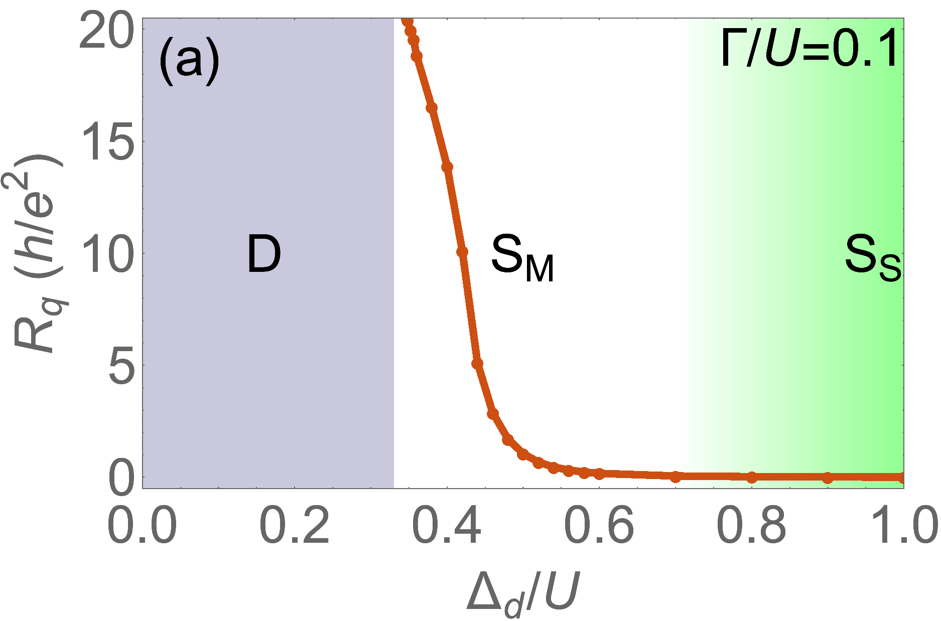
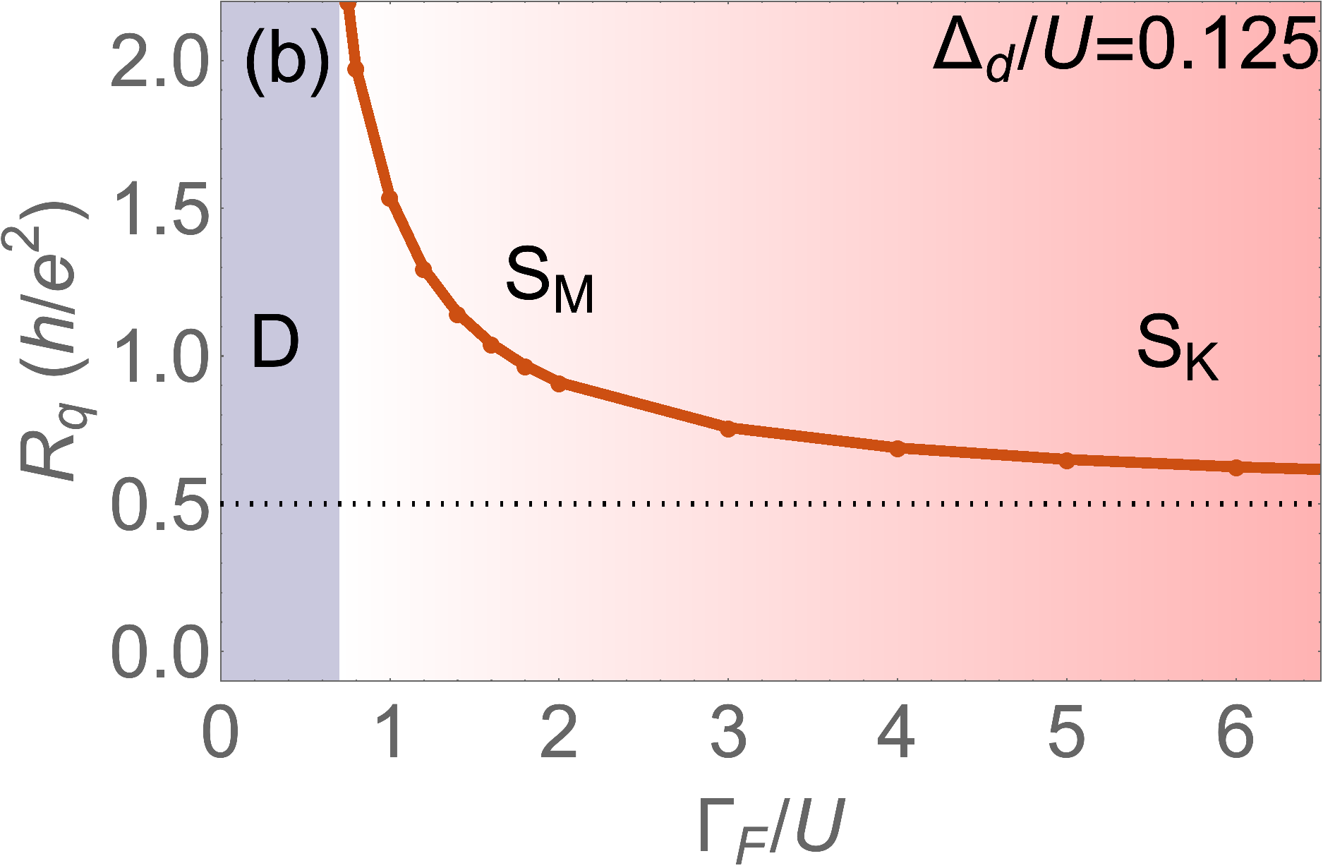
Figure 8: Zero-frequency relaxation resistance $R_{q}(\omega\to 0)$ (a) as functions of $\Delta_{d}$ at $\Gamma_{F}/U=0.1$ along the $bb^{\prime}$ line in Fig. 2 and (b) as functions of $\Gamma_{F}/U$ at $\Delta_{d}/U=0.125$ along the $aa^{\prime}$ line in Fig. 2.

To the contrary, the resistance vanishes in the S_S regime. In the presence of the superconductivity, the particle-hole pairs can be generated via two processes: one is the charge-conserving type ($c_{k\uparrow}^{\dagger}f_{\Uparrow}$ in Eq. (7)) and the other is the pair-tunneling type ($c_{k\uparrow}^{\dagger}f_{\Downarrow}^{\dagger}$). The particle-hole pair amplitudes of the two processes are opposite in sign due to the fermion ordering Lee and Choi (2014). Also, the cancellation is exact in the zero-frequency limit of the particle-hole pairs because the weights from the intermediate virtual states are same for two processes in this limit. On the other hand, $R_{q}$ is observed to saturate toward $h/2e^{2}$ in the S_K regime. For a single-channel Fermi-liquid system, the relaxation resistance is known to have the universal value $h/2e^{2}$ Büttiker et al. (1993a, b), and for the conventional Anderson impurity model in the Kondo regime the resistance becomes $h/4e^{2}$ since there are two spin channels which behave like a composite of two parallel resistors of resistance $h/2e^{2}$ Lee et al. (2011). While our system features the Kondo correlation in this regime, the resistance is $h/2e^{2}$ because there is only a single channel to generate the particle-hole pairs. Finally, in the S_M regime, $R_{q}$ is finite but strongly depends on the values of the parameters: it changes continuously from $R_{q}=\infty$ to the saturation values, as seen in Fig. 8. It is known that Büttiker et al. (1993a, b) the small mesoscopic RC circuit with a single channel should have a universal value $R_{q}=h/2e^{2}$ at zero temperature as long as it is in the Fermi-liquid state. Non-universal value of $R_{q}$ in the S_M, therefore, indicates that the system is in non-Fermi-liquid states, which makes it distinctive from the S_K regime. The microscopic origin of the non-universal value of $R_{q}$ is explained by the fact that the two opposite effects discussed above are partially operative simultaneously: the enhancement of the particle-hole generation due to the high density of states of spin-$\downarrow$ at the Fermi level (near the spin doublet phase) and the cancellation between the charge-conserving and pairing processes (near the S_S regime). The relative strength of the two effects surely depends on the value of the parameters.

VI Conclusion

Using the NRG method, we have studied the triad interplay of superconductivity, ferromagnetism, and Kondo effect all together in a QD coupled to both a superconducting and spin-polarized electrodes as shown schematically in Fig. 1 (a). We have found that unlike the pairwise competition among the three effects, the triad interplay is “cooperative” and leads to a mixed-valence quantum phase transition between doublet and singlet states. The singlet phase is in many respects similar to the mixed-valence state, but connected adiabatically through crossover either to the superconducting state in the limit of strong coupling to the superconductor or to the charge Kondo state in the limit of strong coupling to the spin-polarized lead. Physical explanations and interpretations based on analytic methods such as bosonization, scaling theory, and variational method have been provided. Finally, we have proposed the experimental methods such as the spin-selective tunneling microscopy, measurement of the cross-current correlation and the charge relaxation resistance in order to distinguish the different phases and regimes.

Even though our study has found out the key characteristics of the ferromagnet-quantum dot-superconductor system, it still leaves much room for further studies. First, one can lift the particle-hole symmetry condition used in this work. Then, due to the ferromagnetic proximity effect, it induces an effective Zeeman splitting (or exchange field), which would form subgap states in the dot. Moreover, the breaking of the particle-hole symmetry for spin-$\downarrow$ level is expected to induce an effective Zeeman field for the Kondo model in the S_K regime, shifting the phase boundaries end (b). Secondly, the strong superconductivity condition ($\Delta_{0}\gg U,\Gamma_{S},\Gamma_{F}$) also can be lifted so that the spin Kondo-dominated state ($T_{K}>\Delta_{0}$) can arise. Then, the S_S regime will be replaced by the Kondo state. In this case, one may observe the interesting crossover from the spin Kondo state to the charge Kondo state. Finally, the study can go beyond the equilibrium case by applying a finite bias which is still below the superconducting gap. As discussed in Sec. V, the calculation of the cross-current correlation at finite bias is important for experimental verification. Although the non-equilibrium condition in the presence of a strong interaction is challenging, it is worth doing in the experimental point of view.

Appendix A Variational Method for the Single-Impurity Anderson Model

Here we apply the variational method to the conventional Anderson impurity model described by

$$H_{\mathrm{A}}=\epsilon_{d}\sum_{\sigma}n_{\sigma}+Un_{+}n_{-}+\sum_{k\sigma}\epsilon_{k}\epsilon_{k\sigma}^{\dagger}\epsilon_{k\sigma}\\ {}+\sum_{k\sigma}\left(t_{\sigma}d_{\sigma}^{\dagger}c_{k\sigma}+(h.c.)\right)$$ (30)

in the same way in the text. The conventional Anderson impurity model is different from our model in two points: one is that the lead has two (spin) channels and the second is that the tunneling conserves the spin. The ansatz for spin singlet and doublet states constructed in the similar way as in Eq. (16) is

$$\mathinner{\lvert{\textstyle S}\rangle} =\left(\alpha_{0}+\sum_{k<k_{F},\sigma}\alpha_{k\sigma}d_{\sigma}^{\dagger}c_{k\sigma}+\sum_{k<k_{F},k^{\prime}>k_{F},\sigma}\alpha_{kk^{\prime}\sigma}c_{k^{\prime}\sigma}^{\dagger}c_{k\sigma}\right)\mathinner{\lvert{\textstyle\mathrm{FS}}\rangle}_{0}$$ (31a)

$$\mathinner{\lvert{\textstyle D_{\sigma}}\rangle} =\left(\beta_{0\sigma}d_{\sigma}^{\dagger}+\sum_{k>k_{F}}\beta_{k\sigma}c_{k\sigma}^{\dagger}+\sum_{k>k_{F},k^{\prime}<k_{F},\sigma^{\prime}}\beta_{kk^{\prime}\sigma^{\prime}\sigma}c_{k\sigma}^{\dagger}d_{\sigma^{\prime}}^{\dagger}c_{k^{\prime}\sigma^{\prime}}\right)\mathinner{\lvert{\textstyle\mathrm{FS}}\rangle}_{0}.$$ (31b)

Now we minimize the energy expectation value with respect to these states by applying the Lagrange multiplier method under the normalization constraint $\mathinner{\left\langle{S|S}\right\rangle}=\mathinner{\left\langle{D_{\sigma}|D_{\sigma}}\right\rangle}=1$. Then, one can obtain the following coupled differential equations:

$$\epsilon_{S}\alpha_{0} =-\epsilon_{d}\alpha_{0}+\sum_{k<k_{F},\sigma}t_{\sigma}^{*}\alpha_{k\sigma}$$ (32a)

$$\epsilon_{S}\alpha_{k\sigma} =t_{\sigma}\alpha_{0}-\epsilon_{k}\alpha_{k\sigma}+t_{\sigma}\sum_{k^{\prime}>k_{F}}\alpha_{kk^{\prime}\sigma}$$ (32b)

$$\epsilon_{S}\alpha_{kk^{\prime}\sigma} =t_{\sigma}^{*}\alpha_{k\sigma}+(\epsilon_{k^{\prime}}-\epsilon_{k}-\epsilon_{d})\alpha_{kk^{\prime}\sigma}$$ (32c)

and

$$\epsilon_{D}\beta_{0\sigma} =t_{\sigma}\sum_{k>k_{F}}\beta_{k\sigma}$$ (33a)

$$\epsilon_{D}\beta_{k\sigma} =t_{\sigma}^{*}\beta_{0\sigma}+(\epsilon_{k}-\epsilon_{d})\beta_{k\sigma}+\sum_{k^{\prime}<k_{F},\sigma^{\prime}}t_{\sigma^{\prime}}^{*}\beta_{kk^{\prime}\sigma^{\prime}\sigma}$$ (33b)

$$\epsilon_{D}\beta_{kk^{\prime}\sigma^{\prime}\sigma} =t_{\sigma^{\prime}}\beta_{k\sigma}+(\epsilon_{k}-\epsilon_{k^{\prime}})\beta_{kk^{\prime}\sigma^{\prime}\sigma}.$$ (33c)

Up to the first order (by setting $\alpha_{kk^{\prime}\sigma}=\beta_{kk^{\prime}\sigma^{\prime}\sigma}=0$), the closed-form equations for $\epsilon_{S}$ and $\epsilon_{D}$ are given by

$$\epsilon_{S} =-\epsilon_{d}-\frac{\Gamma_{+}+\Gamma_{-}}{\pi}\ln\left(1+\frac{D}{|\epsilon_{S}|}\right)$$ (34a)

$$\epsilon_{D} =-\frac{\Gamma_{\mu}}{\pi}\ln\left(1+\frac{D}{|\epsilon_{D}|-\epsilon_{d}}\right)$$ (34b)

which is basically same as Eq. (19) except the fact that the dot-lead hybridization is increased since the conventional Anderson impurity model has two spin channels in the lead. Up to the second order, the self-consistent equations for $\epsilon_{S}$ and $\epsilon_{D}$ read

$$\epsilon_{S} =-\epsilon_{d}-\sum_{\sigma}\frac{\Gamma_{\sigma}}{\pi}\int_{0}^{D}\frac{d\epsilon^{\prime}}{\displaystyle\epsilon^{\prime}+|\epsilon_{S}|-\frac{\Gamma_{\sigma}}{\pi}\ln\frac{\epsilon^{\prime}+D+|\epsilon_{S}|+|\epsilon_{d}|}{\epsilon^{\prime}+|\epsilon_{S}|+|\epsilon_{d}|}}$$ (35a)

$$\epsilon_{D} =-\frac{\Gamma_{\sigma}}{\pi}\int_{0}^{D}\frac{d\epsilon^{\prime}}{\displaystyle\epsilon^{\prime}+|\epsilon_{D\sigma}|+|\epsilon_{d}|-\frac{\Gamma_{+}+\Gamma_{-}}{\pi}\ln\frac{\epsilon^{\prime}+D+|\epsilon_{D\sigma}|}{|\epsilon_{d}|+|\epsilon_{D\sigma}|}}.$$ (35b)

References

- López et al. (2002) R. López, R. Aguado, and G. Platero, Phys. Rev. Lett. 89, 136802 (2002).
- Fiete et al. (2002) G. A. Fiete, G. Zarand, B. I. Halperin, and Y. Oreg, Phys. Rev. B 66, 024431 (2002).
- Martinek et al. (2003a) J. Martinek, Y. Utsumi, H. Imamura, J. Barnaś, S. Maekawa, J. König, and G. Schön, Phys. Rev. Lett. 91, 127203 (2003a).
- Martinek et al. (2003b) J. Martinek, M. Sindel, L. Borda, J. Barnaś, J. König, G. Schön, and J. von Delft, Phys. Rev. Lett. 91, 247202 (2003b).
- Choi et al. (2004a) M.-S. Choi, D. Sánchez, and R. López, Phys. Rev. Lett. 92, 056601 (2004a).
- Pasupathy et al. (2004) A. N. Pasupathy, R. C. Bialczak, J. Martinek, J. E. Grose, L. A. K. Doney, P. L. McEuen, and D. C. Ralph, Science 306, 86 (2004).
- Yang et al. (2011) H. Yang, S.-H. Yang, G. Ilnicki, J. Martinek, and S. S. P. Parkin, Phys. Rev. B 83, 174437 (2011).
- Buitelaar et al. (2002) M. R. Buitelaar, T. Nussbaumer, and C. Schönenberger, Phys. Rev. Lett. 89, 256801 (2002).
- Avishai et al. (2003) Y. Avishai, A. Golub, and A. D. Zaikin, Physical Review B 67 (2003).
- Choi et al. (2004b) M.-S. Choi, M. Lee, K. Kang, and W. Belzig, Phys. Rev. B 70, R020502 (2004b).
- Choi et al. (2005) M.-S. Choi, M. Lee, K. Kang, and W. Belzig, Phys. Rev. Lett. 94, 229701 (2005).
- Siano and Egger (2004) F. Siano and R. Egger, Phys. Rev. Lett. 93, 047002 (2004).
- Siano and Egger (2005) F. Siano and R. Egger, Phys. Rev. Lett. 94, 229702 (2005).
- Campagnano et al. (2004) G. Campagnano, D. Giuliano, A. Naddeo, and A. Tagliacozzo, Physica C 406, 1 (2004).
- Sellier et al. (2005) G. Sellier, T. Kopp, J. Kroha, and Y. S. Barash, Phys. Rev. B 72, 174502 (2005).
- Cleuziou et al. (2006) J.-P. Cleuziou, W. Wernsdorfer, V. Bouchiat, T. Ondarçuhu, and M. Monthioux, Nat. Nanotech. 1, 53 (2006).
- Buizert et al. (2007) C. Buizert, A. Oiwa, K. Shibata, K. Hirakawa, and S. Tarucha, Phys. Rev. Lett. 99, 136806 (2007).
- Grove-Rasmussen et al. (2007) K. Grove-Rasmussen, H. I. Jørgensen, and P. E. Lindelof, New Journal of Physics 9, 124 (2007).
- Lim and Choi (2008) J. S. Lim and M.-S. Choi, J. Phys.: Condens. Matt. 20, 415225 (2008).
- Martín-Rodero and Levy Yeyati (2011) A. Martín-Rodero and A. Levy Yeyati, Advances in Physics 60, 899 (2011).
- Franke et al. (2011) K. J. Franke, G. Schulze, and J. I. Pascual, Science 332, 940 (2011).
- Delagrange et al. (2016) R. Delagrange, R. Weil, A. Kasumov, M. Ferrier, H. Bouchiat, and R. Deblock, Physical Review B 93 (2016).
- Delagrange (2016) R. Delagrange, Theses, Université Paris-Saclay (2016).
- Delagrange et al. (2015) R. Delagrange, D. J. Luitz, R. Weil, A. Kasumov, V. Meden, H. Bouchiat, and R. Deblock, Physical Review B 91 (2015).
- Feng and Xiong (2003) J.-F. Feng and S.-J. Xiong, Phys. Rev. B 67, 045316 (2003).
- Cao et al. (2004) X. Cao, Y. Shi, X. Song, S. Zhou, and H. Chen, Physical Review B 70, 235341 (2004).
- Weymann and Wójcik (2015) I. Weymann and K. P. Wójcik, Physical Review B 92, 245307 (2015).
- Hofstetter et al. (2010) L. Hofstetter, A. Geresdi, M. Aagesen, J. Nygård, C. Schönenberger, and S. Csonka, Phys. Rev. Lett. 104, 246804 (2010).
- Zhu et al. (2001) Y. Zhu, Q.-f. Sun, and T.-h. Lin, Phys. Rev. B 65, 024516 (2001).
- Wójcik and Weymann (2014) K. P. Wójcik and I. Weymann, Physical Review B 89, 165303 (2014).
- end (a) For finite polarization, in general the effects of contact-induced exchange field should be considered; see Sahoo et al. (2005); Cottet et al. (2006); Cottet and Choi (2006); Wójcik and Weymann (2014); Weymann and Wójcik (2015). As long as the exchange Zeeman splitting is sufficiently larger than the Kondo temperature, however, they are negligible and our main results are not affected qualitatively even for finite spin polarization.
- end (b) Minchul Lee and Mahn-Soo Choi, to be published elsewhere.
- Volkov et al. (1995) A. F. Volkov, P. H. C. Magnée, B. J. van Wees, and T. M. Klapwijk, Physica C 242, 261 (1995).
- McMillan (1968) W. L. McMillan, Phys. Rev. 175, 537 (1968).
- Žitko and Pruschke (2009) R. Žitko and T. Pruschke, Physical Review B 79, 85106 (2009).
- Žitko and Simon (2011) R. Žitko and P. Simon, Physical Review B 84, 195310 (2011).
- Campo and Oliveira (2005) V. Campo and L. Oliveira, Physical Review B 72, 104432 (2005).
- Yoshida et al. (1990) M. Yoshida, M. Whitaker, and L. Oliveira, Physical Review B 41, 9403 (1990).
- Wilson (1975a) K. Wilson, Reviews of Modern Physics 47, 773 (1975a).
- Krishna-murthy et al. (1980a) H. R. Krishna-murthy, J. W. Wilkins, and K. G. Wilson, Phys. Rev. B 21, 1003 (1980a).
- Bulla et al. (2008) R. Bulla, T. Costi, and T. Pruschke, Reviews of Modern Physics 80, 395 (2008).
- Wilson (1975b) K. G. Wilson, Rev. Mod. Phys. 47, 773 (1975b).
- Krishna-murthy et al. (1980b) H. R. Krishna-murthy, J. W. Wilkins, and K. G. Wilson, Phys. Rev. B 21, 1044 (1980b).
- Büttiker et al. (1993a) M. Büttiker, A. Prêtre, and H. Thomas, Physical Review Letters 70, 4114 (1993a).
- Büttiker et al. (1993b) M. Büttiker, H. Thomas, and A. Prêtre, Physics Letters A 180, 364 (1993b).
- Lee et al. (2011) M. Lee, R. López, M.-S. Choi, T. Jonckheere, and T. Martin, Physical Review B 83, 201304 (2011).
- Lee and Choi (2014) M. Lee and M.-s. Choi, Physical Review Letters 113, 076801 (2014).
- Matveev (1991) K. Matveev, Sov. Phys. JETP 72 (1991).
- Iftikhar et al. (2015) Z. Iftikhar, S. Jezouin, A. Anthore, U. Gennser, F. D. Parmentier, A. Cavanna, and F. Pierre, Nature 526, 233 (2015).
- Anderson (1961) P. W. Anderson, Phys. Rev. 124, 41 (1961).
- Varma and Yafet (1976) C. M. Varma and Y. Yafet, Phys. Rev. B 13, 2950 (1976).
- Jefferson (1977) J. H. Jefferson, Journal of Physics C: Solid State Physics 10, 3589 (1977).
- Haldane (1978) F. D. M. Haldane, Phys. Rev. Lett. 40, 416 (1978), erratum: ibid, 911 (1978).
- Ramakrishnan and Sur (1982) T. V. Ramakrishnan and K. Sur, Phys. Rev. B 26, 1798 (1982).
- Gunnarsson and Schönhammer (1983) O. Gunnarsson and K. Schönhammer, Phys. Rev. B 28, 4315 (1983).
- Anderson (1970) P. W. Anderson, J. Phys. C 3, 2436 (1970).
- de Jong and Beenakker (1995) M. de Jong and C. Beenakker, Physical Review Letters 74, 1657 (1995).
- Sahoo et al. (2005) S. Sahoo, T. Kontos, J. Furer, C. Hoffmann, M. Gräber, A. Cottet, and C. Schönenberger, Nature Phys. 1, 99 (2005).
- Cottet et al. (2006) A. Cottet, T. Kontos, S. Sahoo, H. T. Man, M.-S. Choi, W. Belzig, C. Bruder, A. Morpurgo, and C. Schönenberger, Semicond. Sci. Technol. 21, S78 (2006).
- Cottet and Choi (2006) A. Cottet and M.-S. Choi, Phys. Rev. B 74, 235316 (2006).