Measuring the Wilson depression of sunspots using the divergence-free condition of the magnetic field vector
Abstract
Context. The Wilson depression is the difference in geometric height of unit continuum optical depth between the sunspot umbra and the quiet Sun. Measuring the Wilson depression is important for understanding the geometry of sunspots. Current methods suffer from systematic effects or need to make assumptions on the geometry of the magnetic field. This leads to large systematic uncertainties of the derived Wilson depressions.
Aims. We aim at developing a robust method for deriving the Wilson depression that only requires the information about the magnetic field that is accessible from spectropolarimetry, and that does not rely on assumptions on the geometry of sunspots or on their magnetic field.
Methods. Our method is based on minimizing the divergence of the magnetic field vector derived from spectropolarimetric observations. We focus on large spatial scales only in order to reduce the number of free parameters.
Results. We test the performance of our method using synthetic Hinode data derived from two sunspot simulations. We find that the maximum and the umbral averaged Wilson depression for both spots determined with our method typically lies within 100 km of the true value obtained from the simulations. In addition, we apply the method to Hinode observations of a sunspot. The derived Wilson depression ( km) is consistent with results typically obtained from the Wilson effect. We also find that the Wilson depression obtained from using horizontal force balance gives 110 - 180 km smaller Wilson depressions than both, what we find and what we deduce directly from the simulations. This suggests that the magnetic pressure and the magnetic curvature force contribute to the Wilson depression by a similar amount.
Key Words.:
sunspots – Sun: photosphere – Sun: magnetic fields1 Introduction
The geometric height at which unity continuum optical depth is reached is depressed within sunspots relative to the quiet Sun. This so-called Wilson depression (Wilson & Maskelyne, 1774) is caused by a lower opacity within the sunspot due to the lower temperature and a reduced gas pressure. The magnetic pressure and the curvature force of the strong magnetic field of sunspots balance this reduced gas pressure with the gas pressure of the surrounding quiet Sun. The connection between the Wilson depression and the strength and geometry of the magnetic field makes the Wilson depression an important quantity for understanding the structure of sunspots. In particular, it is not known by how much the curvature force of the magnetic field contributes to stabilizing the sunspot.
Unfortunately, the Wilson depression remains one of the more poorly known parameters of sunspots. Several studies have tried inferring the Wilson depression by making use of the horizontal force balance between the sunspot and the surrounding quiet Sun. However, since it is unknown by how much the curvature force contributes to the force balance, an accurate estimate of the Wilson depression with this method is not possible. Depending on the assumed influence of the curvature force, the derived Wilson depression lies in the range between 400-1000 km (Solanki et al., 1993; Martínez Pillet & Vázquez, 1993; Mathew et al., 2004).
The Wilson depression can also be estimated geometrically when the sunspot approaches the limb (i. e. via the Wilson effect). However, this method is influenced by radiative transfer or changes of the size of the umbra and penumbra with height (see, e.g., the discussion in Solanki, 2003). Hence, the Wilson depression cannot be inferred very accurately when using this method. Gokhale & Zwaan (1972) derived an average Wilson depression of km based on the Wilson effect. In contrast, Prokakis (1974) measured a significantly larger Wilson depression of km with large spots having a higher Wilson depression ( km) than small spots ( km). However, later results ( km) obtained by Balthasar & Wöhl (1983) are in better agreement with those of Gokhale & Zwaan (1972).
Here we present an alternative method for measuring the Wilson depression that does not need to make any assumptions on the geometry of the magnetic field in sunspots or on the structure of the sunspot. Our method is based on imposing the divergence-free condition on the magnetic field vector deduced from the inversion of observed Stokes profiles. This approach has already been used by Puschmann et al. (2010) to derive the small-scale corrugation of the layer of a small patch within the penumbra of a sunspot. Here, we modify this method to provide the large-scale corrugation of the layer within the entire sunspot. We first perform a test of the method: we use it to derive the Wilson depression from synthetic Hinode observations generated from two MHD simulations of sunspots (Rempel, 2012, 2015). After that we apply it to one spot observed with Hinode. We also compare our results with the Wilson depression derived using the pressure method.
2 Data
| Parameter | Simulation 1 | Simulation 2 | AR 10923 |
|---|---|---|---|
| area [Mm2] | 938 | 650 | 2572 |
| [Gauss] | 4247 | 5194 | 4341 |
| [Gauss] | 3143 | 3624 | 2911 |
| [K] | 3896 | 3608 | 3579 |
| [K] | 4607 | 4325 | 4116 |
2.1 Synthetic Hinode data
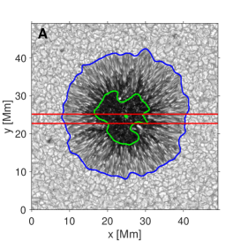
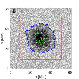
We generate synthetic Hinode data starting from two MHD simulations of sunspots by Rempel (2012, 2015) computed with the MURaM code (Vögler et al., 2005). Simulation run 1 has a size of with a resolution of ( pixels). Simulation run 2 has a size of with a resolution of ( pixels). Figure 1 shows continuum intensity images and Table 1 lists some parameters of the spots (the area of the spots, the maximum and the average magnetic field in the umbra at , and the minimum and average temperature in the umbra at ). We define the inner and outer boundary of the penumbra as 30% and 90% of the continuum intensity level of the quiet Sun, respectively, after smoothing the continuum images with a 2D Gaussian with km.
We compute line profiles of the pair of Fe I lines at Å and Å for all Stokes parameters from these simulations using the SPINOR code (Frutiger et al., 2000); which uses the STOPRO routines for the forward calculation (Solanki, 1987) for . In order to save computation time, we only compute the line profiles for a narrow strip across the sunspot for simulation run 1 (indicated by the red lines in the left panel in Figure 1). For simulation run 2, we use the full field-of-view (FOV). We then degrade the data to the spectral resolution of Hinode SOT/SP and rebin the data to the pixel size of Hinode SOT/SP (). We do not convolve the data with the optical point-spread function (PSF) since an inversion with the spatially coupled version of SPINOR (van Noort, 2012; van Noort et al., 2013) would remove the influence of the PSF from the data anyway. Note that the sunspot AR 10923 observed by Hinode and analyzed here, was inverted with the spatially coupled version of SPINOR and we intend to apply this technique mainly to data inverted in the same manner. Finally, we add normally distributed noise to all four Stokes parameters with a signal-to-noise ratio that is proportional to the square root of the intensity and that reaches an average value of 1000 in the continuum.
2.2 Hinode observations of AR 10923
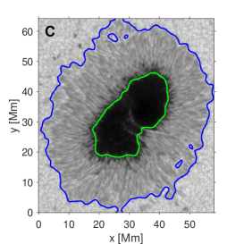
We use spectropolarimetric observations of AR 10923 made on 14 November 2006 in the Fe I line pair at Å and Å from the spectropolarimeter on the Solar Optical Telescope (SOT/SP, Kosugi et al., 2007; Lites, 2007; Ichimoto et al., 2008; Lites et al., 2013) onboard the Hinode spacecraft. At that time, this active region was located close to disk center (, see panel C in Figure 1). The SOT/SP provides the full set of Stokes parameters along both spectral lines with a pixel sampling of . This spot exhibits two filaments stretching far into the umbra, nearly splitting the umbra in two parts. This spot is significantly larger than the two simulated spots, however, the magnetic field in the umbra is weaker (see Table 1).
3 Deriving the atmospheric conditions
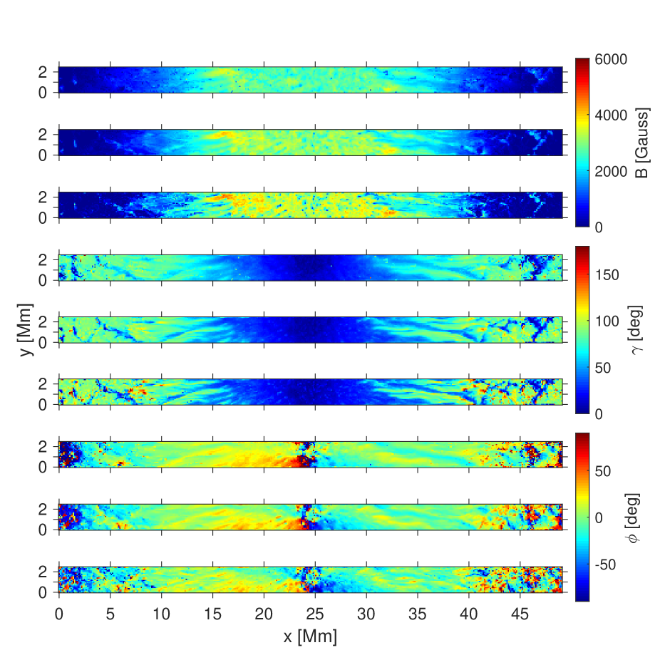
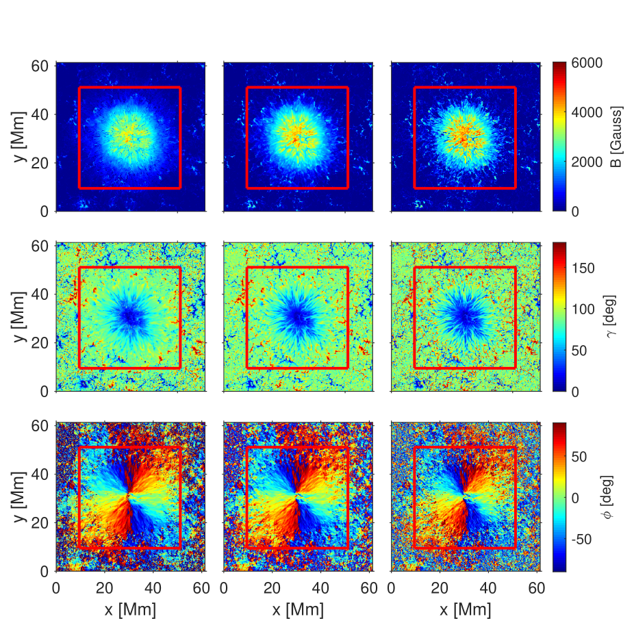
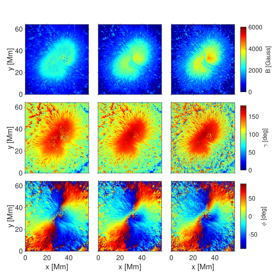
We derive the atmospheric parameters of both, the two simulated spots and AR 10923, by inverting the maps of the Stokes parameters with the SPINOR code under the assumption of local thermodynamic equilibrium (LTE). In case of the Hinode observations, we use the spatially coupled version of SPINOR (van Noort, 2012; van Noort et al., 2013). The synthetic data are inverted using the non-coupled version of SPINOR since we did not take into account the PSF when generating the synthetic data. For all three spots, we set three nodes in optical depth, placed at . Figures 2 to 4 show the results of the inversion for the magnetic field strength , the inclination , and the azimuth for all the spots at these optical depths. Using a spline interpolation, we then remap the results of the inversion on an equidistant grid in ranging from to with a sampling of .
Afterward, we resolve the azimuthal ambiguity by using the Non-Potential Magnetic Field Computation method (NPFC, Georgoulis, 2005). We can test the performance of the NPFC code with the help of the synthetic data. In most cases, the code resolves the ambiguity correctly within the sunspot. However, the code sometimes fails in regions where the magnetic field vector is almost exactly parallel to the line-of-sight. This occurs predominantly at optical depths where the inversion is less accurate. We address this issue by applying the NPFC code only to the data at . We then successively resolve the ambiguity at greater and lower heights by demanding the magnetic field vector to vary smoothly with height. We select the solution of the ambiguity, where the magnetic field vector is the closest to the one in the adjacent layer, where we have already resolved the ambiguity. This leads to an accurate disambiguation within the sunspot. In the surroundings of the sunspots, however, the NPFC code fails in many cases to find the correct solution, even at .
4 Measuring the Wilson depression
4.1 The method
We determine the geometric height of the layer of the sunspot in a similar way as introduced by Puschmann et al. (2010), who could infer the geometrical height of the surface in an inverted atmosphere of a small patch of the penumbra of a sunspot observed with Hinode. Their method is based on the divergence-free condition of the magnetic field vector and on ensuring force balance. These two conditions are not fulfilled in an inverted atmosphere since the unknown height of the layer causes an offset in the geometric height scale of the individual pixels. However, both the divergence of the magnetic field and the deviations from force balance are minimized when shifting the atmosphere at each pixel by the corresponding height of the surface. Hence, this approach allows to infer the Wilson depression. Puschmann et al. (2010) use the following merit function:
| (1) |
The sum is over all the pixels in the images (indicated by the indices and ). The first term consists of the residual force . Here, is the current density, is the magnetic field vector, is the density, is the surface gravity of the Sun, and is the gas pressure. The influence of flows on the force balance is neglected. The second term in the merit function is the divergence of the magnetic field. The relative contributions of the two terms are balanced by the coefficients and .
The magnetic field vector and all other atmospheric parameters in the merit function depend on the geometric height . This height scale has two contributions. The first one is the -scale of the stratification relative to the layer of each pixel, which is provided by the inversion. The second one is the height of the layer at each pixel (i. e. the Wilson depression ), which we want to determine:
| (2) |
Changing at the individual pixels corresponds to shifting the inverted atmosphere vertically. The merit function has its minimum when the inverted atmospheres for all pixels are aligned with respect to each other, i. e., when is the corrugation of the surface. The alignment of the individual atmospheres can be evaluated at different heights relative to the surface. Puschmann et al. (2010) used km and set as the height used to compute the merit function for an arbitrary pixel. They used a genetic algorithm for minimizing the merit function.
Here, we want to extend the method of Puschmann et al. (2010) to derive the corrugations of the layer of the entire spot. This is not straightforward since the Wilson depression at each pixel is a free parameter in the merit function. So, the number of free parameters becomes extremely large when applying this method to the entire spot. We reduce the number of free parameters by restricting the analysis to the large-scale corrugation of the layer. An efficient way to achieve this is to write the Wilson depression as a Fourier series of the horizontal wavenumbers and and then drop the terms above a maximum wavenumber in the Fourier series of , therefore removing the small-scale corrugations. Now, the number of free parameters does not correspond to the number of pixels anymore, but it depends on the maximum wavenumber that is considered. This approach allows us to reduce the number of free parameters in the merit function significantly without affecting the determination of the large-scale Wilson depression.
However, neglecting small-scale corrugations of the layer affects the divergence of the magnetic field, especially on small spatial scales. We address this problem by writing the merit function in Fourier space using Parseval’s theorem:
| (3) |
Here, the symbol indicates a 2D discrete Fourier transform (in the - and in the -direction), defined as
| (4) |
The parameters and are the number of pixels along the -axis and the -axis, respectively. The indices and indicate the dimensionless wavenumber indices and are connected to the physical wavenumber by the relation in case of the -direction with being the spatial resolution. Contrary to Puschmann et al. (2010), we do not include the force terms in our merit function. In our case, including the force terms leads to a less accurate determination of the Wilson depression. This is caused by neglecting advection () in the force balance (spectropolarimetry can only measure the line-of-sight velocity, not the full velocity vector). In the penumbra of the two simulated spots, the advection term reaches a similar magnitude as the Lorentz force due to the Evershed and the reverse Evershed flow. Hence, ignoring advection causes the force term in the merit function not to be sensitive to the large-scale Wilson depression anymore.
All terms in the merit function are positive, meaning that the divergence has to be zero at all spatial scales in order to minimize the merit function. So, one can restrict the analysis to the large spatial scales of the divergence only, which are less affected by neglecting the small-scale corrugations of the layer. Both for the Wilson depression and for the divergence of the magnetic field vector, we only consider spatial scales up to maximum dimensionless wavenumbers and . This decreases the effective spatial resolution significantly (given by the wavelength corresponding to the indices and ). When using a maximum dimensionless wavenumber , for example, we retrieve an effective spatial resolution of 14 Mm for the part of simulation run 2 that is highlighted by the red box in Figure 1.
We filter both, the Wilson depression and the magnetic field vector in Fourier space to include only the information about large spatial scales. Hence, a map of the large-scale magnetic field at a fixed geometric height is affected by the filtering in two ways. Ignoring the small-scale corrugations of the layer causes an error in the derived magnetic field vector if the magnetic field varies strongly with height at a given pixel. Afterwards, variations of the magnetic field itself on small spatial scales are removed. This filtering should remove most of the errors introduced by neglecting the small-scale corrugations of the layer.
This assumption can be tested using the simulated sunspots. We compute maps of all three components of the magnetic field vector at a fixed geometrical height (200 km above the mean height of the layer) from simulation run 2 for two different cases. In the first case, we derive the magnetic field on a grid in geometric height that includes small-scale corrugations of the surface, in the second case, we neglect corrugations above a maximum dimensionless wavenumber . Afterwards, we also remove the signal at spatial scales above or from the maps of the magnetic field vector. The correlation coefficient between these two sets of maps of the magnetic field vector is for all three components of the magnetic field vector, indicating that the small-scale corrugations of the surface do not have a strong influence on the large-scale magnetic field. Using this approach leads to the following expression for the merit function:
| (5) | ||||
| (6) |
Here, and are the Fourier transforms of and , respectively. Again, the geometric height consists of the relative height above the surface and the Wilson depression . We evaluate the merit function around a fixed reference height and require the derived Wilson depression to have a mean value of zero. Like Puschmann et al. (2010), we minimize our merit function using a genetic algorithm. We run the genetic algorithm ten times and use the solution which minimizes the merit function the most. After running the genetic algorithm, we define as the height of the surface averaged over the part of the FOV that has a distance of at least 7 Mm to the sunspot. This minimum distance is necessary because the height of the surface can be depressed in the close surroundings of the sunspot.
Our method relates the magnetic field vector in the quiet Sun and in the umbra at the same geometric height. This requires an accurate measurement of the magnetic field vector over a broad range in height since sunspots have a Wilson depression of a few 100 km. So, in order to derive reliable estimates of the Wilson depression, the magnetic field vector retrieved by the inversion needs to be reliable over a broad range in height around the reference height . Errors in the inversion occur predominantly at high optical depths (we do not consider data at heights km) and at very low optical depths. We choose to be as small as possible while ensuring that all inferred heights are greater than our threshold of 85 km. The inversion also suffers from systematic errors, such as the assumption of hydrostatic equilibrium. In the simulation data, this is a good approximation in granules and in the umbra but not so good in the intergranular lanes and in the penumbra. Errors occurring on small spatial scales should have limited influence though, due to our focus on large spatial scales.
We perform our analysis in Fourier space. This means that the magnetic field vector and the derived Wilson depression have periodic boundary conditions when expressing them in Fourier space. This is a good approximation when the field of view also contains the surroundings of the sunspot, where the magnetic field and the Wilson depression are significantly lower than within the spot.
| Spot | Method | [km] | [km] | [km] | [km] | [km] | [km] |
| Simulation 1 | True solution (full res.) | 719 | 552 | 286 | |||
| True solution (filtered) | 606 | 546 | 284 | ||||
| Divergence | 702 | 539 | 58 | 264 | 57 | 22 | |
| pressure (full res.) | 598 | 424 | 128 | 163 | 124 | 33 | |
| pressure (filtered) | 482 | 418 | 129 | 167 | 118 | 23 | |
| Simulation 2 | True solution (full res.) | 880 | 602 | 253 | |||
| True solution (filtered) | 644 | 559 | 252 | ||||
| Divergence | 591 | 478 | 95 | 296 | 81 | 47 | |
| pressure (full res.) | 791 | 489 | 115 | 128 | 126 | 34 | |
| pressure (filtered) | 548 | 449 | 111 | 130 | 123 | 22 | |
| AR 10923 | Divergence | 720 | 600 | 195 | |||
| pressure (full res.) | 742 | 427 | 82 | ||||
| pressure (filtered) | 555 | 414 | 82 |
4.2 Synthetic Hinode data
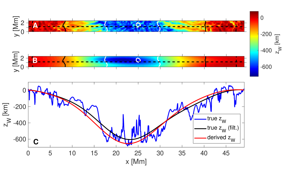
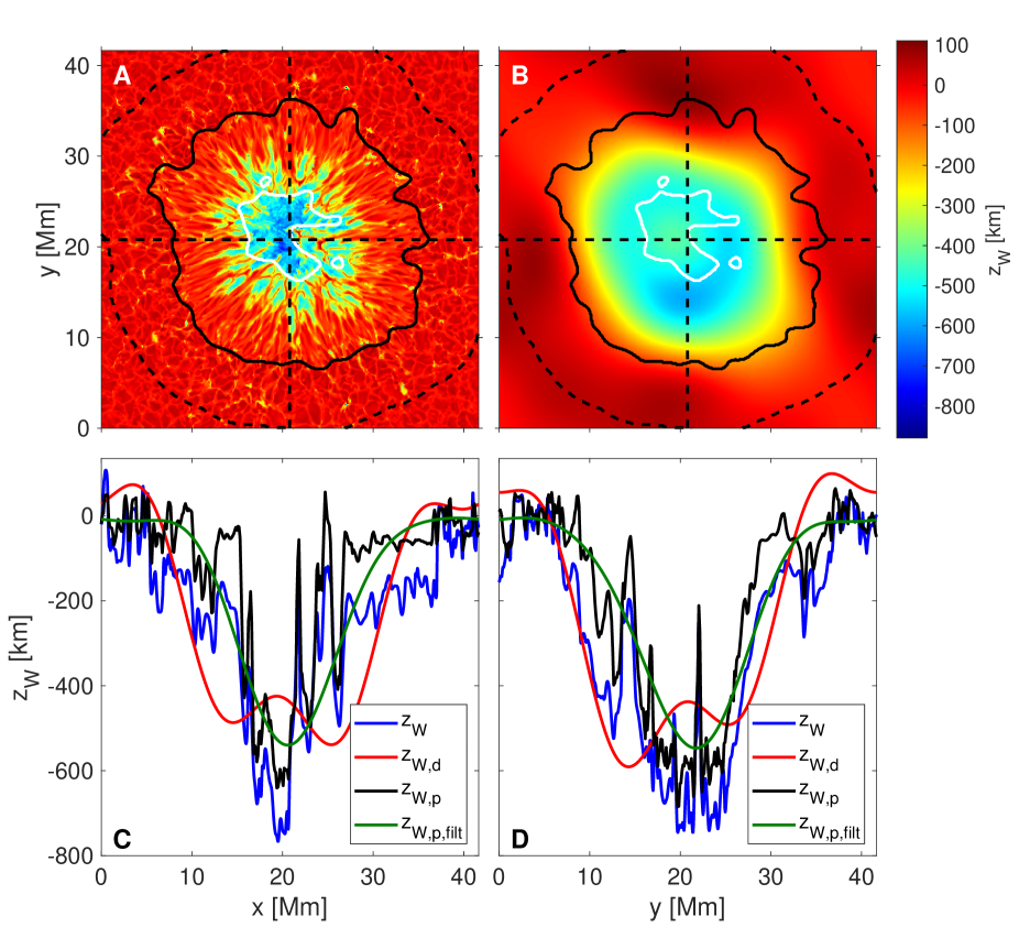
Figures 5 and 6 show the Wilson depressions derived from synthetic Hinode data for the two simulated sunspots. For comparison, we also show the true values of the Wilson depression for both spots which were inferred by resampling the MHD cubes on a grid in optical depth using SPINOR. We set as the height of the surface averaged over the region of the FOV that has a distance of at least 7 Mm to the outer boundary of the penumbra (see dashed black contours in Figures 5 and 6). In Table 2, we quantitatively compare the Wilson depression inferred by our method with the true solution and results from the pressure method (see Sect. 4.3). We list the maximum Wilson depression () and its average over the umbra () and over the penumbra (), both for the full spatial resolution (called “full res.” in the table) and after degrading it to the resolution of our method (“filtered” in the table). We also derive error estimates of the Wilson depression for the umbra (), the penumbra (), and the area outside the sunspot (). We derive these errors from maps of the absolute value of the difference between our solutions and the true Wilson depression (after degrading it to the spatial resolution of our derived Wilson depressions). We then define the errors to be the average of this difference map over the respective region of the spot.
For spot 1, we compute the Wilson depression only along a slice across the sunspot to limit the computation time due to the large number of pixels. Within this slice, the magnetic field vector is not periodic in the -direction, in particular the component. Since this non-periodic boundary condition would affect the filtering in Fourier space, we compute the divergence using the full spatial resolution in the -direction. However, we do apply Fourier filtering in the -direction. We express the Wilson depression in Fourier space, though, in order to reduce the number of free parameters (, ). The main differences between our solution and the true Wilson depression occur on small spatial scales, which we do not consider in our method. We degrade the true solution to the same spatial resolution as our derived Wilson depression (black curve in the bottom panel of Figure 5) in order to remove the influence of the differences in spatial resolution. Our derived Wilson depression is generally in good agreement with the degraded true solution, but the maximum Wilson depression is km larger than the degraded true solution (see Table 2). The averages of the Wilson depression over the umbra and the penumbra are in good agreement, though. In both cases, the mean absolute difference between our solution and the true Wilson depression is of the order of 60 km.
This error estimate is affected both by uncertainties introduced by the inversion of the Stokes parameters and by the stability of the genetic algorithm. We evaluate the stability of the minimization by computing the standard deviation of the Wilson depression inferred by running the genetic algorithm ten times. The resulting errors (34 km for the maximum Wilson depression and 17 km for the average over the umbra) are significantly smaller than the difference between the derived and the true Wilson depression. This suggests that the error is dominated by uncertainties in the inversion.
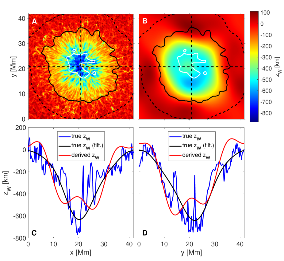
Spot 2 exhibits a very complex Wilson depression in the umbra with changes of several 100 km on small spatial scales (see Figure 6). These small-scale corrugations cannot be resolved by our method (here we use ). Again, for better comparison, we smooth the true solution in order to account for this effect. Afterwards, both the maximum Wilson depression and its averages over the umbra and the penumbra are in good agreement (see Table 2). A remarkable difference between our solution and the true solution occurs at Mm. At this position, there is a filament stretching to the umbra and the layer is located a few 100 km higher than in the surrounding umbra. Our method finds an extremely large Wilson depression at this location, in contradiction to the true solution. This error in the derived Wilson depression is probably caused by uncertainties in the inversion. Along the filament, the magnetic field changes strongly with height (by up to 2000 Gauss over a range of 100 km at around ). This height dependency cannot be described correctly by the inversion. This feature not only affects the Wilson depression locally but also in the surrounding umbra. This is because the spatial resolution of our method is very low and because the Fourier transform is non-local (a perturbation of the signal at a given point also affects distant points after filtering in Fourier space). Again, we compute the mean absolute value of the difference between our derived Wilson depression and the true solution. The differences are roughly a factor larger than the ones for spot 1 and much larger than the uncertainty introduced by the genetic algorithm (13 km for the maximum Wilson depression and 9 km for the average over the umbra), in agreement with the findings from spot 1.
The inferred Wilson depression depends on the parameters of the merit function. Apart from the Wilson depression, the merit function (Eq. 6) depends on the range of spatial scales that is considered (given by and ) and the height above () where the merit function is evaluated. As stated in the previous section, the height is a crucial parameter since it determines, what range in height (and optical depth) is used for inferring the Wilson depression. We choose the reference height to be as small as possible while ensuring that all inferred heights are greater than our threshold of 85 km (350 km for spot 1, 300 km for spot 2). For larger reference heights, the derived Wilson depression becomes less reliable. We also restrained the solution to low wavenumbers. Larger wavenumbers should be avoided since in that case the solution for the Wilson depression is more likely to exhibit an oscillatory behavior, especially in the quiet Sun.
4.3 Comparison with the pressure method
For comparison, we also derive the Wilson depression by demanding horizontal force balance between the sunspot and the surrounding quiet Sun (Martínez Pillet & Vázquez, 1993; Solanki et al., 1993; Mathew et al., 2004). The reduced gas pressure inside the umbra is compensated by the Lorentz force of the strong magnetic field. After a few assumptions, such as radial symmetry of the magnetic field vector, no magnetic field in the azimuthal direction and a negligible Evershed flow (Maltby, 1977), this can be expressed as
| (7) |
Here, refers to the center of the umbra and to a point in the quiet Sun. The second term on the right-hand side, is the curvature integral:
| (8) |
Equation 7 can be used to infer the Wilson depression of a sunspot by comparing the measured total pressure (gas pressure plus magnetic pressure) at some optical depth with the pressure stratification of a reference model atmosphere of the quiet Sun (which extends at least to the depth of the Wilson depression). The derived Wilson depression depends on the curvature integral, which cannot directly be inferred from the observations. Commonly, one assumes (see e.g., Mathew et al., 2004).
We apply this method to both simulated sunspots. We use a horizontal average of a quiet-sun region from simulation run 2 as the reference atmosphere and extract the pressure and the magnetic field from the inversions at . The resulting Wilson depressions are in the range km, when averaging over the umbra (see Table 2), in good agreement with the results from previous studies for , which lay in the range 400-450 km (Martínez Pillet & Vázquez, 1993; Solanki et al., 1993; Mathew et al., 2004). Figure 7 compares the Wilson depression inferred from this method for simulation run 2 with our results based on the divergence of the magnetic field and the true solution.
The pressure method results in a Wilson depression which is about 110 km smaller than the true value for the simulations. This suggests that the curvature integral is positive in both spots. We obtain the curvature integral by assuming that the difference between the true Wilson depression and the one obtained from the pressure method is due to the curvature integral neglected by the pressure method. For the spot in simulation 2, an error in the Wilson depression of 110 km corresponds to in the umbra. This is about half of the value of the magnetic pressure in the umbra ().
The inferred value of is in good agreement with the curvature integral derived directly from the MHD cube. The curvature integral depends on height, between km and km, varies between and . At greater heights, it becomes negative, reaching at km. This change of sign is caused by the vertical derivative of the radial component of the magnetic field in Eq. 8. The strength of reaches its maximum at around and decreases towards larger or smaller heights, causing a change of sign of its vertical derivative.
In the penumbra, the pressure method significantly underestimates the Wilson depression (by more than 100 km for the spot in simulation run 2). This is caused by using only the vertical component of the magnetic field when estimating the magnetic pressure. In the penumbra, the magnetic field is predominantly horizontal, meaning that the magnetic pressure and, hence, also the Wilson depression is underestimated when using only.
4.4 Real Hinode data: case study of AR 10923
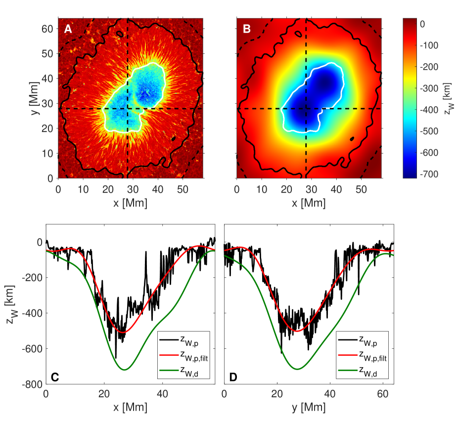
We also tested the performance of our method on the Hinode observations of AR 10923 (see Figure 8 and Table 2). Again, we used a maximum dimensionless wavenumber , which corresponds to an effective spatial resolution of Mm in the -direction and Mm in the -direction. The resulting Wilson depression looks similar to the one of the simulated spots, although the average Wilson depression is by km deeper. It displays two distinct local maxima, where the Wilson depression exceeds 700 km. These maxima occur in regions with strong magnetic field (see top row of Figure 4). These two regions are separated by a filament, along which the Wilson depression is reduced by km. The Wilson depression smoothly decreases from the center of the umbra towards the outer penumbral boundary. The height of the surface is more or less constant outside the sunspot, which is to be expected at the large spatial scales considered here.
Unfortunately, we cannot derive a reliable estimate of the error of the Wilson depression for this spot. As found from the simulated spots (Section 4.2) the main errors in arise from uncertainties in the inversions. Obtaining the errors in inverted values is never straightforward, also from the spatially coupled inversion scheme of van Noort (2012); van Noort et al. (2013), which was used to invert this spot. We expect that the uncertainty is similar to or larger than for the synthetic data, i. e. roughly 95 km or larger.
The Wilson depression derived using the pressure method (see Figure 8 and Table 2) is significantly smaller (by about 180 km) than the one based on our method, suggesting that the curvature integral is positive in this spot, as well. Assuming the deduced via the divergence method to be correct, we retrieve . This is higher than the pressure from the vertical component of the magnetic field () in the umbra at . The high value of of AR 10923 is consistent with typical values found in other spots, while the results for the simulated spots are lower than what has been reported before. Solanki et al. (1993) estimate the curvature integral to be within the range for the sunspot that they studied. The value we find lies within this range.
5 Discussion
We could successfully reproduce the Wilson depression of two simulated sunspots by minimizing the divergence of the magnetic field. We also applied this method to a sunspot observed with Hinode (AR 10923) and derived a Wilson depression that is consistent with the results statistically provided by some studies of the Wilson effect ( km, Gokhale & Zwaan, 1972). Our results suggest that the pressure due to the vertical component of the magnetic field and the curvature integral contribute by a similar amount to the horizontal force balance within sunspots, as has already been suggested by previous investigations (Martínez Pillet & Vázquez, 1993; Solanki et al., 1993; Mathew et al., 2004). The Wilson depression of the sunspot simulations by Rempel (2012, 2015) is smaller by km than the one of AR 10923. In the simulated spots, the curvature integral is significantly lower than the pressure due to the vertical component of the magnetic field, leading to a lower Wilson depression. This might be caused by the different geometry of the simulated spots compared to AR 10923 (see Table 1). The simulated spots exhibit a slightly stronger magnetic field but they are significantly smaller than the AR 10923 spot.
The main limitation of our method is that it requires a reliable inversion of the full magnetic field vector over a broad range in height. In the umbra, our method requires an estimate of the magnetic field up to km above the surface. The lines used in this study are not very sensitive at these height and so, the magnetic field is predominantly extrapolated from lower layers. Observations of multiple spectral lines with a broad range of formation heights are needed in order to retrieve a better inversion (as is planned, e. g., with the upcoming Sunrise III mission). Systematic errors also arise from the assumption of LTE and hydrostatic equilibrium in the inversion, although these are likely small compared with the uncertainty resulting from the inversions. Also, modeling the height dependency of atmospheric parameters with splines is not always a good representation of the true atmosphere, especially when there are strong gradients with height. In addition, the -ambiguity of the Zeemann-effect needs to be resolved accurately across the entire spot at all optical depths. Fortunately, some of these inaccuracies of the inversion occur on small spatial scales, so that their influence on large spatial scales should be limited. For example, as shown in Section 4.1, neglecting the small-scale corrugations of the layer has only a small influence on the large-scale divergence of the magnetic field. A detailed determination of the errors in the spatially coupled inversion is beyond the scope of this paper. We therefore use the tests made with the synthetic data as a rough guide to the total error.
The Wilson depression derived from the synthetic Hinode data exhibits an error of the order of km. In case of real observations, the error is probably somewhat higher. The synthetic data were generated using the same radiative transfer code and the same line parameters as were used for the inversion. Hence, the inversion of the synthetic data is likely to be more accurate than for real observations. Bearing these arguments in mind, we assign a preliminary error of 100 km to the Wilson depression derived from the Hinode observations.
The estimated error of our method is mainly statistical in nature. Any systematic component is significantly lower than the one of the Wilson effect or of the pressure method. As explained in the introduction, the values of the Wilson depression derived using the Wilson effect vary by more than 1000 km between different studies in a systematic manner. In case of the pressure method, the inferred Wilson depression depends on the assumed value of the curvature integral.
Our method is limited to the large-scale corrugations of the surface. Measuring the Wilson depression with a higher spatial resolution requires including more Fourier coefficients in the Fourier series of the Wilson depression, which affects the minimization of the merit function. In addition, the divergence of the magnetic field is dominated by the largest spatial scales. When evaluating the divergence of the magnetic field for AR 10923 on a corrugated grid in geometrical height (300 km above at each pixel), 76% of the total variance of the divergence of the magnetic field occur within the range of spatial scales that we considered in Section 4.4 (). Hence, the merit function is not very sensitive to smaller spatial scales, at least when considering entire sunspots.
Acknowledgements.
This work benefited from the Hinode sunspot database at MPS, created by Gautam Narayan. This project has received funding from the European Research Council (ERC) under the European Union’s Horizon 2020 research and innovation programme (grant agreement No 695075) and has been supported by the BK21 plus program through the National Research Foundation (NRF) funded by the Ministry of Education of Korea.References
- Balthasar & Wöhl (1983) Balthasar, H. & Wöhl, H. 1983, Sol. Phys., 88, 71
- Frutiger et al. (2000) Frutiger, C., Solanki, S. K., Fligge, M., & Bruls, J. H. M. J. 2000, A&A, 358, 1109
- Georgoulis (2005) Georgoulis, M. K. 2005, ApJ, 629, L69
- Gokhale & Zwaan (1972) Gokhale, M. H. & Zwaan, C. 1972, Sol. Phys., 26, 52
- Ichimoto et al. (2008) Ichimoto, K., Lites, B., Elmore, D., et al. 2008, Sol. Phys., 249, 233
- Kosugi et al. (2007) Kosugi, T., Matsuzaki, K., Sakao, T., et al. 2007, Sol. Phys., 243, 3
- Lites (2007) Lites, B. W. 2007, in Astronomical Society of the Pacific Conference Series, Vol. 369, New Solar Physics with Solar-B Mission, ed. K. Shibata, S. Nagata, & T. Sakurai, 579
- Lites et al. (2013) Lites, B. W., Akin, D. L., Card, G., et al. 2013, Sol. Phys., 283, 579
- Maltby (1977) Maltby, P. 1977, Sol. Phys., 55, 335
- Martínez Pillet & Vázquez (1993) Martínez Pillet, V. & Vázquez, M. 1993, A&A, 270, 494
- Mathew et al. (2004) Mathew, S. K., Solanki, S. K., Lagg, A., et al. 2004, A&A, 422, 693
- Prokakis (1974) Prokakis, T. 1974, Sol. Phys., 35, 105
- Puschmann et al. (2010) Puschmann, K. G., Ruiz Cobo, B., & Martínez Pillet, V. 2010, ApJ, 720, 1417
- Rempel (2012) Rempel, M. 2012, ApJ, 750, 62
- Rempel (2015) Rempel, M. 2015, ApJ, 814, 125
- Solanki (1987) Solanki, S. K. 1987, Ph.D. Thesis No. 8309 (ETH, Zürich)
- Solanki (2003) Solanki, S. K. 2003, A&A Rev., 11, 153
- Solanki et al. (1993) Solanki, S. K., Walther, U., & Livingston, W. 1993, A&A, 277, 639
- van Noort (2012) van Noort, M. 2012, A&A, 548, A5
- van Noort et al. (2013) van Noort, M., Lagg, A., Tiwari, S. K., & Solanki, S. K. 2013, A&A, 557, A24
- Vögler et al. (2005) Vögler, A., Shelyag, S., Schüssler, M., et al. 2005, A&A, 429, 335
- Wilson & Maskelyne (1774) Wilson, A. & Maskelyne, N. 1774, Philosophical Transactions of the Royal Society of London Series I, 64, 1