Very strong evidence in favor of quantum mechanics
and against local hidden variables from a Bayesian analysis

Abstract

The data of four recent experiments — conducted in Delft, Vienna, Boulder, and Munich with the aim of refuting nonquantum hidden-variables alternatives to the quantum-mechanical description — are evaluated from a Bayesian perspective of what constitutes evidence in statistical data. We find that each of the experiments provides strong, or very strong, evidence in favor of quantum mechanics and against the nonquantum alternatives. This Bayesian analysis supplements the previous non-Bayesian ones, which refuted the alternatives on the basis of small p-values, but could not support quantum mechanics.
Keywords: quantum mechanics, local hidden variables, Bayesian methods, evidence in statistical data

I Introduction

Four recent experiments in Delft Delft , Vienna Vienna , Boulder Boulder , and Munich Munich tested the variants of Bell’s inequality Bell:64 introduced by Clauser et al. Clauser+3:69 and Eberhard Eberhard:93 . The shared aim of these experiments was the refutation of descriptions in terms of local hidden variables (LHV) that Bell and others had proposed as an alternative to the description offered by quantum mechanics (QM). Upon extracting small p-values from the respective data, with values between $3.74\times 10^{-31}$ (Vienna) and $0.039$ (Delft), each of the four groups of scientists concluded that their data refute the LHV hypothesis. Putting aside all other caveats about, objections against, and other issues with the use of p-values Evans:p-value ; ASA:16 ; Benjamin+71:17 , let us merely note that the use of p-values can only make a case against LHV but not in support of QM. Yet, a clear-cut demonstration that the data give evidence in favor of QM is surely desirable.

We present here an evaluation of the data of the four experiments that shows that there is very strong evidence in favor of QM and also against LHV. Our analysis does not rely on p-values or any other concepts of frequentist statistics. We use Bayesian logic and measure evidence — in favor of alternatives or against them — by comparing the posterior with the prior probabilities of the alternatives to be distinguished.

The basic notion is both simple and natural Evans:15 : If an alternative is more probable in view of the data than before acquiring them, then the data provide evidence in favor of this alternative; and, conversely, if an alternative is less probable after taking note of the data than before, then the data give evidence against this alternative.

In our analysis, we only employ this principle of evidence and no particular measure for quantifying the strength of the evidence strength . As it happens, all alternatives save one are extremely improbable in view of the data so that the evidence in favor of the privileged alternative is overwhelming, and a quantification of the strength of the evidence is not needed here.

While Bell’s inequality and its variants are central to the design of the experiments, they play no role in our evaluation of the data. What matters are the probabilities of occurrence of the various measurement outcomes in the experiments. As discussed in Sec. III, the permissible probabilities make up an eight-dimensional set. It is composed of three subsets: one accessible only by QM, another only by LHV, and the third by both; see Fig. 1. We then ask Do the data provide evidence in favor of or against each of the three subsets? and, from the data of each of the four experiments, we find strong evidence for the QM-only subset and against the other two.

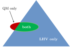
Figure 1: Symbolic sketch of the eight-dimensional set of permissible probabilities. The points inside the ellipse symbolize probabilities accessible by quantum mechanics (QM); the triangle encloses the probabilities permitted by local hidden variables (LHV). There are no QM probabilities in the blue portion of the LHV set, and no LHV probabilities in the red part of the QM set. The green overlap region contains the probabilities that are possible both for QM and LHV.

An essential part of the Bayesian analysis is the choice of prior — the assignment of prior probabilities to the three regions in Fig. 1, thereby accounting for our prior knowledge about the experiment and the assumptions behind its design. If we were to strictly follow the rules of Bayesian reasoning, we would endow the set of QM-permitted probabilities with a prior close to 100% and allocate a very tiny prior to the subset of LHV-only probabilities. For, generations of physicists have accumulated a very large body of solid experimental and theoretical knowledge that makes us extremely confident that QM is correct. Not one observed effect contradicts the predictions of QM, while there is not a single documented phenomenon in support of all those speculations about LHV. In fact, this was already the situation in the mid 1960s when Bell published Ref. Bell:64 and gave a physical interpretation to an inequality known to Boole a century before Boole:62 .

Moreover, for the evaluation of the data from the four experiments, a by-the-rules prior, namely a properly elicited prior, would have to reflect our strong conviction that the experimenters managed to implement the experiment as planned in a highly reliable fashion, with the desired probabilities from the QM-only subset. Accordingly, we really should assign a very large prior probability to the “QM only” region symbolized in Fig. 1, a much smaller one to the “both” region, and an even smaller one to the “LHV only” region.

Such a prior, however, could bias the data evaluation in favor of QM and against LHV. Therefore, we deliberately violate the rules and use a prior that treats QM and LHV on equal footing; see Sec. V. To demonstrate that our choice of prior is not biased toward QM, we check for such a bias and confirm that there is none; more about this in Sec. V.3. Yet, all this tilting of the procedure does not help the LHV case: The data speak clearly and loudly that QM rules and LHV are out.

This contributes also to the development of Bayesian methodology, inasmuch as we demonstrate that the subjective biases inherent in a Bayesian statistical analysis through, for example, the choice of the prior, can be assessed a priori. To the best of our knowledge this is one of the first applications of this type of computation to ensure that such choices are not producing foregone conclusions.

We recall the experimental scheme common to all four experiments (Sec. II) and the ways in which the probabilities of detecting the various events are parameterized in the QM formalism or by LHV (Sec. III). This is followed by a discussion of how the difference between the prior and the posterior content of a region gives evidence in favor of this region or against it (Sec. IV). Then we explain our choice of prior on the eight-dimensional set of permissible probabilities — permitted either by QM or by LHV (Sec. V); more specifically, we define the prior by the algorithm that yields the large sample of permissible probabilities needed for the Monte Carlo integrations over the three regions symbolized in Fig. 1.

Then, having thus set the stage, we present, as a full illustration of the reasoning and methodology, the detailed account of the various aspects of our evaluation of the data recorded in one run of the Boulder experiment (Sec. VI.1). This includes the estimation, from the data, of an experimental parameter for which the value given in Ref. Boulder is not accurate. While an accurate value is not needed for calculating the p-value reported in Ref. Boulder , it is crucial for the QM account of the experiment. The results of processing the data from three other runs of the Boulder experiment are reported in Sec. VI.2. The evaluation of the data from three runs of the Vienna experiment also requires the estimation of the analogous parameter (Sec. VII.1) whereas there is no need for that in the context of the experiments conducted in Delft and Munich (Sec. VII.2).

All four experiments separately provide strong evidence in favor of QM and against LHV. Jointly, they convey the very clear message that this verdict is final.

II Experimental scheme

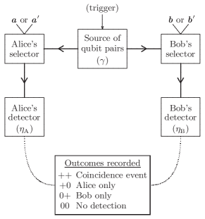
Figure 2: Upon receiving a trigger signal, the source of qubit pairs equips Alice and Bob with one qubit each; the success probability for this initial step is $\gamma$. The qubits are detected with the respective efficiencies $\eta^{\ }_{\mathrm{A}}$ and $\eta^{\ }_{\mathrm{B}}$ if they pass a selection process, specified by $\vecfont{a}$ or $\vecfont{a}^{\prime}$ for Alice’s qubit and by $\vecfont{b}$ or $\vecfont{b}^{\prime}$ for Bob’s qubit. For each trigger signal, we record whether there was a coincidence event, or only Alice or only Bob observed a detector click, or both did not. Data are collected for all four settings: $\vecfont{a}$ or $\vecfont{a}^{\prime}$ together with $\vecfont{b}$ or $\vecfont{b}^{\prime}$.

The four experiments realize variations of one theme; see Fig. 2. Upon receiving a trigger signal, the source of qubit pairs equips Alice and Bob with one qubit each; the success probability for this is denoted by $\gamma$. Alice chooses one of two settings, denoted by $\vecfont{a}$ and $\vecfont{a}^{\prime}$, for her selector in front of her qubit detector, which fires with efficiency $\eta^{\ }_{\mathrm{A}}$. Likewise Bob chooses between settings $\vecfont{b}$ and $\vecfont{b}^{\prime}$ for his selector and then detects the selected qubits with efficiency $\eta^{\ }_{\mathrm{B}}$. For each trigger signal, the outcome is recorded and counts as an event of one of four kinds: a “$++$ event” if Alice’s and Bob’s detectors both fire; a “$+0$ event” if Alice’s detector fires and Bob’s does not; a “$0+$ event” if Alice’s detector does not fire and Bob’s does; or a “$00$ event” if both detectors do not fire. The data $D$ consist of the number of events observed of the four kinds, for the four settings available by choosing $\vecfont{a}$ or $\vecfont{a}^{\prime}$ and $\vecfont{b}$ or $\vecfont{b}^{\prime}$; together there are sixteen counts, such as $n^{(ab^{\prime})}_{0+}$ for the $0+$ events in the setting with $\vecfont{a}$ and $\vecfont{b}^{\prime}$, and

$$D=\Bigl{(}n^{(ab)}_{++},n^{(ab)}_{+0},\dots,n^{(ab^{\prime})}_{0+},\dots,n^{(a^{\prime}b^{\prime})}_{00}\Bigr{)}$$ (1)

reports the data for one run of the experiment as a 16-element string of natural numbers. Their sum

$$N=n^{(ab)}_{++}+n^{(ab)}_{+0}+\cdots+n^{(ab^{\prime})}_{0+}+\cdots+n^{(a^{\prime}b^{\prime})}_{00}$$ (2)

is the total number of trigger signals.

Table 1 lists the parameters of the four experiments fn:data . The Vienna and Boulder experiments exploit the polarization qubits of photon pairs generated by down-conversion processes that happen rarely ($\gamma\ll 1$). The unit vectors $\vecfont{a}$, $\vecfont{a}^{\prime}$ and $\vecfont{b}$, $\vecfont{b}^{\prime}$ that specify the selections refer to the orientation of polarization filters, and the detectors register the photons that are let through.

The qubits in the Delft and Munich experiments are in superpositions of hyperfine states of two atoms in spatially separated traps. The preparation of the initial state is achieved by entanglement swapping and is, therefore, heralded so that $\gamma=1$ in these event-ready setups. The selection and detection are implemented by probing for a chosen superposition, specified by the Bloch vectors $\vecfont{a}$, $\vecfont{a}^{\prime}$ and $\vecfont{b}$, $\vecfont{b}^{\prime}$.

Table 1: The parameters of the four experiments: the trigger–to–qubit-pair conversion probability $\gamma$; the angle $\theta^{\ }_{\mathrm{A}}$ between Alice’s settings; the angle $\theta^{\ }_{\mathrm{B}}$ between Bob’s settings; Alice’s detection efficiency $\eta^{\ }_{\mathrm{A}}$; Bob’s detection efficiency $\eta^{\ }_{\mathrm{B}}$; number $N$ of trigger signals for two runs (Delft, Munich), three runs (Vienna), or four runs (Boulder).

Experiment	$\gamma$	$\theta^{\ }_{\mathrm{A}}$	$\theta^{\ }_{\mathrm{B}}$	$\eta^{\ }_{\mathrm{A}}$	$\eta^{\ }_{\mathrm{B}}$	$N$
Delft Delft ; Delft-2nd	1	$90^{\circ}$	$80.6^{\circ}$	0.971	0.963	245
						228
Vienna Vienna	0.003 5	$64^{\circ}$	$64^{\circ}$	0.786	0.762	3 843 698 536
						3 502 784 150
						9 994 696 192
Boulder Boulder	0.000 5	$60.2^{\circ}$	$60.2^{\circ}$	0.747	0.756	175 647 100
						527 164 272
						886 791 755
						1 244 205 032
Munich Munich ; fn:Munich-eta	1	$90^{\circ}$	$90^{\circ}$	0.975	0.975	27 885
						27 683

Since the physics is independent of the coordinate systems adopted for the description, we can regard $\vecfont{a}$ and $\vecfont{a}^{\prime}$ as vectors in the $xz$ plane of the Bloch ball for Alice’s qubit, and likewise $\vecfont{b}$ and $\vecfont{b}^{\prime}$ are in the $xz$ plane for Bob’s qubit. All that matters is the angle $\theta^{\ }_{\mathrm{A}}$ between $\vecfont{a}$ and $\vecfont{a}^{\prime}$, and the angle $\theta^{\ }_{\mathrm{B}}$ between $\vecfont{b}$ and $\vecfont{b}^{\prime}$. Our choice of coordinate systems is then such that

$${\left.\begin{array}[]{c}\vecfont{a}\\ \vecfont{a}^{\prime}\end{array}\right\}} = \pm\vecfont{e}_{x}\sin\bigl{(}\tfrac{1}{2}\theta^{\ }_{\mathrm{A}}\bigr{)}+\vecfont{e}_{z}\cos\bigl{(}\tfrac{1}{2}\theta^{\ }_{\mathrm{A}}\bigr{)}\,,$$ (5)

$${\left.\begin{array}[]{c}\vecfont{b}\\ \vecfont{b}^{\prime}\end{array}\right\}} = \pm\vecfont{n}_{x}\sin\bigl{(}\tfrac{1}{2}\theta^{\ }_{\mathrm{B}}\bigr{)}+\vecfont{n}_{z}\cos\bigl{(}\tfrac{1}{2}\theta^{\ }_{\mathrm{B}}\bigr{)}\,,$$ (8)

where $\vecfont{e}_{x}$, $\vecfont{e}_{y}$, $\vecfont{e}_{z}$ are the cartesian unit vectors for Alice’s qubit and $\vecfont{n}_{x}$, $\vecfont{n}_{y}$, $\vecfont{n}_{z}$ are those for Bob’s. Table 1 reports the respective values of $\theta^{\ }_{\mathrm{A}}$ and $\theta^{\ }_{\mathrm{B}}$.

A comment is in order about the table entries for $\theta^{\ }_{\mathrm{A}}$ and $\theta^{\ }_{\mathrm{B}}$. The information given in Refs. Delft ; Vienna ; Boulder ; Munich is in terms of angles with respect to a reference direction, such as the setting of a wave plate relative to the conventional direction of vertical polarization. This tells us, for each setting, the magnitudes of the probability amplitudes in the superposition of vertical and horizontal polarizations but not their complex phases. It appears that the experimenters assumed that there are no relative phases, and this assumption leads to the values of $\theta^{\ }_{\mathrm{A}}$ and $\theta^{\ }_{\mathrm{B}}$ in Table 1. When the assumption is not made, we get a range of values for some of the $\theta^{\ }_{\mathrm{A}}$s and $\theta^{\ }_{\mathrm{B}}$s, such as ${25.9^{\circ}-4.2^{\circ}<\frac{1}{2}\theta^{\ }_{\mathrm{A}}<25.9^{\circ}+4.2^{\circ}}$ in the Boulder experiment. It is possible to estimate $\theta^{\ }_{\mathrm{A}}$ and $\theta^{\ }_{\mathrm{B}}$ from the data (in a manner analogous to that of Sec. VI.1.1) and we performed such an estimation for the Boulder data in Table 2 below, with the outcome that $\theta^{\ }_{\mathrm{A}}=60.2^{\circ}$ is reasonable. We regard this as assurance that there are no relative phases to be concerned about.

Another comment concerns the uncertainties of the $\eta^{\ }_{\mathrm{A}}$s and $\eta^{\ }_{\mathrm{B}}$s, and of the $\theta^{\ }_{\mathrm{A}}$s and $\theta^{\ }_{\mathrm{B}}$s in Table 1, such as $\eta^{\ }_{\mathrm{A}}=74.7\pm 0.3\%$ and $\eta^{\ }_{\mathrm{B}}=75.6\pm 0.3\%$ for the Boulder experiment Boulder . While the evaluation of the data reported in Secs. VI and VII refers to the parameter values in Table 1, we also used slightly different values for comparison and found that our conclusions are not affected at all.

III Permissible probabilities

For each setting $S=ab$ or $ab^{\prime}$ or $a^{\prime}b$ or $a^{\prime}b^{\prime}$, we have the four probabilities $p^{(S)}_{++}$, $p^{(S)}_{+0}$, $p^{(S)}_{0+}$, and $p^{(S)}_{00}$ of recording the respective events for the next trigger signal. These have unit sum,

$$\sum_{\alpha,\beta=+,0}p^{(S)}_{\alpha\beta}=1\,,$$ (9)

but are otherwise unrestricted. Accordingly, the quartets of probabilities for one setting $S$ compose the whole standard probability 3-simplex. There are four simplices of this kind, one for each setting, which are linked because Alice’s detection probabilities do not depend on Bob’s setting,

$$p_{+}^{(a)} \equiv p^{(ab)}_{++}+p^{(ab)}_{+0}=p^{(ab^{\prime})}_{++}+p^{(ab^{\prime})}_{+0}\,,$$

$$p_{+}^{(a^{\prime})} \equiv p^{(a^{\prime}b)}_{++}+p^{(a^{\prime}b)}_{+0}=p^{(a^{\prime}b^{\prime})}_{++}+p^{(a^{\prime}b^{\prime})}_{+0}\,,$$ (10)

and Bob’s detection probabilities do not depend on Alice’s setting,

$$p_{+}^{(b)} \equiv p^{(ab)}_{++}+p^{(ab)}_{0+}=p^{(a^{\prime}b)}_{++}+p^{(a^{\prime}b)}_{0+}\,,$$

$$p_{+}^{(b^{\prime})} \equiv p^{(ab^{\prime})}_{++}+p^{(ab^{\prime})}_{0+}=p^{(a^{\prime}b^{\prime})}_{++}+p^{(a^{\prime}b^{\prime})}_{0+}\,.$$ (11)

These are the so-called “no signaling” conditions.

Together, then, the sixteen probabilities $p^{(S)}_{\alpha\beta}$ obey eight constraints and, therefore, the probability space is eight-dimensional. The regions sketched in Fig. 1 are regions in this eight-dimensional probability space. It is fully parameterized by the four probabilities in Eqs. (III) and (III) and the four null-event probabilities $p^{(S)}_{00}$, as illustrated by

$$p^{(ab)}_{++} = p_{+}^{(a)}+p_{+}^{(b)}+p^{(ab)}_{00}-1\,,$$

$$p^{(ab)}_{+0} = 1-p^{(ab)}_{00}-p_{+}^{(b)}\,,$$

$$p^{(ab)}_{0+} = 1-p^{(ab)}_{00}-p_{+}^{(a)}$$ (12)

for setting $S=ab$.

III.1 QM probabilities

In the description offered by QM, a trigger signal results in a qubit pair with probability $\gamma$ and yields nothing with probability $1-\gamma$. With $\rho$ denoting the statistical operator of the qubit pair, $\boldsymbol{\sigma}$ the Pauli vector operator of a qubit, and $\boldsymbol{1}$ the identity operator, we have

$$p^{(a)}_{+} = \gamma\eta^{\ }_{\mathrm{A}}\textnormal{tr}{{\left\{\tfrac{1}{2}(\boldsymbol{1}+\vecfont{a}\cdot\boldsymbol{\sigma})\otimes\boldsymbol{1}\,\rho\right\}}}\,,$$

$$p^{(a^{\prime})}_{+} = \gamma\eta^{\ }_{\mathrm{A}}\textnormal{tr}{{\left\{\tfrac{1}{2}(\boldsymbol{1}+\vecfont{a}^{\prime}\cdot\boldsymbol{\sigma})\otimes\boldsymbol{1}\,\rho\right\}}}\,,$$

$$p^{(b)}_{+} = \gamma\eta^{\ }_{\mathrm{B}}\textnormal{tr}{{\left\{\boldsymbol{1}\otimes\tfrac{1}{2}(\boldsymbol{1}+\vecfont{b}\cdot\boldsymbol{\sigma})\,\rho\right\}}}\,,$$

$$p^{(b^{\prime})}_{+} = \gamma\eta^{\ }_{\mathrm{B}}\textnormal{tr}{{\left\{\boldsymbol{1}\otimes\tfrac{1}{2}(\boldsymbol{1}+\vecfont{b}^{\prime}\cdot\boldsymbol{\sigma})\,\rho\right\}}}$$ (13)

for Alice’s and Bob’s individual probabilities Munich-dark , and the null-event probabilities are

$$p^{(ab)}_{00} = \gamma\,\mathrm{tr}\Bigl{\{}\bigl{[}\boldsymbol{1}-\eta^{\ }_{\mathrm{A}}\tfrac{1}{2}(\boldsymbol{1}+\vecfont{a}\cdot\boldsymbol{\sigma})\bigr{]}$$ (14)

$$\hphantom{\gamma\mathrm{tr}\Bigl{\{}}\otimes\bigl{[}\boldsymbol{1}-\eta^{\ }_{\mathrm{B}}\tfrac{1}{2}(\boldsymbol{1}+\vecfont{b}\cdot\boldsymbol{\sigma})\bigr{]}\rho\Bigr{\}}+(1-\gamma)\quad$$

and analogous expressions for $p^{(ab^{\prime})}_{00}$, $p^{(a^{\prime}b)}_{00}$, and $p^{(a^{\prime}b^{\prime})}_{00}$.

Owing to their small $\gamma$ values, the probabilities in the Vienna and Boulder experiments occupy only a very small portion of the linked 3-simplices because the probabilities are bounded by

$$p^{(S)}_{++}\leq\gamma\eta^{\ }_{\mathrm{A}}\eta^{\ }_{\mathrm{B}}\,,\quad p^{(S)}_{00}\geq 1-\gamma\,,$$

$$p^{(a)}_{+},p^{(a^{\prime})}_{+}\leq\gamma\eta^{\ }_{\mathrm{A}}\,,\quad p^{(b)}_{+},p^{(b^{\prime})}_{+}\leq\gamma\eta^{\ }_{\mathrm{B}}\,.$$ (15)

For the Delft and Munich experiments, which have $\gamma=1$ and $\eta^{\ }_{\mathrm{A}},\eta^{\ }_{\mathrm{B}}\lesssim 1$, no major portions of the 3-simplices are excluded.

The set of permissible QM probabilities, enclosed by the symbolic ellipse in Fig. 1, is made up by the probabilities $p^{(S)}_{\alpha\beta}$ obtained from all thinkable $\rho$s in accordance with Eqs. (III)–(14). Each statistical operator $\rho$ is represented by a density matrix — a hermitian, nonnegative, unit-trace $4\times 4$ matrix. As a consequence of Eq. (5), the $p^{(S)}_{\alpha\beta}$s are linear combinations of the expectation values of the eight operators

$$\sigma_{x}\otimes\boldsymbol{1}\,,\quad\sigma_{z}\otimes\boldsymbol{1}\,,\quad\boldsymbol{1}\otimes\sigma_{x}\,,\quad\boldsymbol{1}\otimes\sigma_{z}\,,$$

$$\sigma_{x}\otimes\sigma_{x}\,,\quad\sigma_{z}\otimes\sigma_{x}\,,\quad\sigma_{x}\otimes\sigma_{z}\,,\quad\sigma_{z}\otimes\sigma_{z}\,,\qquad$$ (16)

all represented by real $4\times 4$ matrices if we employ the standard real $2\times 2$ matrices for $\sigma_{x}$ and $\sigma_{z}$. Therefore, only the real parts of the matrix elements of $\rho$ matter, and we only need to consider $\rho$s represented by real density matrices, which make up a nine-dimensional convex set. The ninth parameter is the expectation value of $\sigma_{y}\otimes\sigma_{y}=(\sigma_{x}\otimes\sigma_{z})(\sigma_{z}\otimes\sigma_{x})$.

III.2 LHV probabilities

In the LHV reasoning, the sequence “first create a qubit pair, then select, finally detect” of Sec. III.1 is meaningless; all that has meaning is “detection event after trigger signal” Brunner+4:14 . There are no sequential processes controlled by the hidden variables step-by-step, they control the overall process. Therefore, the trigger-to-pair probability $\gamma$ and the detection probabilities $\eta^{\ }_{\mathrm{A}}$, $\eta^{\ }_{\mathrm{B}}$, which are central to the correct application of Born’s rule in Eqs. (III.1) and (14), play no role when relating the $p^{(S)}_{\alpha\beta}$s to hidden variables.

Following Wigner Wigner:70 and others (see, for example, Refs. Fine:82 ; Kaszlikowski:00 ), we parameterize the LHV probabilities in terms of sixteen hypothetical probabilities $w(\alpha\alpha^{\prime}\beta\beta^{\prime})$ from the 15-simplex,

$$\mathop{\sum_{\alpha,\alpha^{\prime}=+,0}}_{\beta,\beta^{\prime}=+,0}\!\!w(\alpha\alpha^{\prime}\beta\beta^{\prime})=1\quad\mbox{with}\enskip w(\alpha\alpha^{\prime}\beta\beta^{\prime})\geq 0\,.$$ (17)

Here, $w(\alpha\alpha^{\prime}\beta\beta^{\prime})$ is the fictitious joint probability of obtaining, for the next trigger signal, result $\alpha$ for Alice’s setting $\vecfont{a}$, and result $\alpha^{\prime}$ for her setting $\vecfont{a}^{\prime}$, and result $\beta$ for Bob’s setting $\vecfont{b}$, and also result $\beta^{\prime}$ for his setting $\vecfont{b}^{\prime}$ (never mind that she has setting $\vecfont{a}$ or $\vecfont{a}^{\prime}$ and he has $\vecfont{b}$ or $\vecfont{b}^{\prime}$). The eight marginal probabilities

$$p^{(a)}_{+} = \sum_{\alpha^{\prime},\beta,\beta^{\prime}}\!w(\mathnormal{+}\alpha^{\prime}\beta\beta^{\prime})\,,\quad p^{(a^{\prime})}_{+}=\sum_{\alpha,\beta,\beta^{\prime}}\!w(\alpha\mathnormal{+}\beta\beta^{\prime})\,,$$

$$p^{(b)}_{+} = \sum_{\alpha,\alpha^{\prime},\beta^{\prime}}\!w(\alpha\alpha^{\prime}\mathnormal{+}\beta^{\prime})\,,\quad p^{(b^{\prime})}_{+}=\sum_{\alpha,\alpha^{\prime},\beta}\!w(\alpha\alpha^{\prime}\beta\mathnormal{+})\,,$$

$$p^{(ab)}_{00} = \sum_{\alpha^{\prime},\beta^{\prime}}w(0\alpha^{\prime}0\beta^{\prime})\,,\quad p^{(ab^{\prime})}_{00}=\sum_{\alpha^{\prime},\beta}w(0\alpha^{\prime}\beta 0)\,,$$

$$p^{(a^{\prime}b)}_{00} = \sum_{\alpha,\beta^{\prime}}w(\alpha 00\beta^{\prime})\,,\quad p^{(a^{\prime}b^{\prime})}_{00}=\sum_{\alpha,\beta}w(\alpha 0\beta 0)$$ (18)

then determine the sixteen $p^{(S)}_{\alpha\beta}$s in accordance with Eq. (III).

The hidden probabilities $w(\alpha\alpha^{\prime}\beta\beta^{\prime})$ control all aspects of the experiment, and they are such that they mislead us into regarding QM as correct. That is, the LHV probabilities $p^{(S)}_{\alpha\beta}$ should have as many properties of the QM probabilities as possible. Therefore, we require that all inequalities in Eq. (III.1) are respected by the LHV probabilities. Through these inequalities, then, the values of $\eta^{\ }_{\mathrm{A}}$, $\eta^{\ }_{\mathrm{B}}$, and $\gamma$, which are properties of the experimental apparatus, enter the LHV formalism. Accordingly, the set of permissible LHV probabilities, enclosed by the symbolic triangle in Fig. 1, is made up by the probabilities $p^{(S)}_{\alpha\beta}$ obtained from all thinkable $w(\alpha\alpha^{\prime}\beta\beta^{\prime})$s in accordance with Eqs. (III) and (III.2), subject to the constraints in Eq. (III.1).

Note that, as a consequence of the different values of $\eta^{\ }_{\mathrm{A}}$, $\eta^{\ }_{\mathrm{B}}$, and $\gamma$, we have different sets of permissible probabilities for the four experiments. Symbolically, there are several different ellipses and several different triangles in Fig. 1.

Note also that the “LHV only” region is not empty. For example, if we choose $w(\alpha\alpha^{\prime}\beta\beta^{\prime})=0$ for all hidden probabilities except for $w(\mathnormal{+}\mathnormal{+}\mathnormal{+}\mathnormal{+})=\gamma\eta^{\ }_{\mathrm{A}}\eta^{\ }_{\mathrm{B}}$ and $w(0000)=1-\gamma\eta^{\ }_{\mathrm{A}}\eta^{\ }_{\mathrm{B}}$, then the constraints of Eq. (III.1) are obeyed and we get $p_{++}^{(S)}=\gamma\eta^{\ }_{\mathrm{A}}\eta^{\ }_{\mathrm{B}}$ for all four settings; there is no statistical operator $\rho$ for which the QM probabilities of Eqs. (III.1) and (14) are like this. And any $\rho$ for which a Bell-type inequality, such as $p^{(ab^{\prime})}_{+0}+p^{(a^{\prime}b)}_{0+}+p^{(a^{\prime}b^{\prime})}_{++}\geq p^{(ab)}_{++}$, is violated will give probabilities in the “QM only” region.

IV Prior and posterior content; evidence

We write $(\mathrm{d}p)\,w_{0}(p)$ for the prior probability assigned to the infinitesimal vicinity of a point $p=\bigl{(}p^{(ab)}_{++},\dots,p^{(a^{\prime}b^{\prime})}_{00}\bigr{)}$ in the probability space, where the differential element

$$(\mathrm{d}p)=\mathrm{d}p^{(ab)}_{++}\,\mathrm{d}p^{(ab)}_{+0}\,\cdots\mathrm{d}p^{(a^{\prime}b^{\prime})}_{00}\,w^{\ }_{\mathrm{cstr}}(p)$$ (19)

incorporates the constraints that restrict $p$ to the set of permissible values, symbolized by the union of the regions enclosed by the ellipse and the triangle in Fig. 1. In particular, we have $w^{\ }_{\mathrm{cstr}}(p)=0$ when Eqs. (9)–(III) are not obeyed. Other constraints result from the nonnegativity of the statistical operator and the hidden probabilities, and from the restrictions imposed by Eq. (III.1). Although there are algorithms for checking whether the constraints are obeyed by any given $p$, we do not have an explicit expression for $w^{\ }_{\mathrm{cstr}}(p)$; we also do not need one.

While $w^{\ }_{\mathrm{cstr}}(p)$ depends on the parameters of the experiments, with different constraints for the four experiments because they differ in the values of $\theta^{\ }_{\mathrm{A}}$, $\theta^{\ }_{\mathrm{B}}$, $\eta^{\ }_{\mathrm{A}}$, $\eta^{\ }_{\mathrm{B}}$, and $\gamma$ (see Table 1), the factor $w_{0}(p)$ reflects what we know about the experiments before the data are acquired. Our choice for $w_{0}(p)$ is discussed in Sec. V; here, we shall assume that a certain choice has been made.

Then

$$S_{\mathcal{R}}=\int\limits_{\mathcal{R}}(\mathrm{d}p)\,w_{0}(p)$$ (20)

is the prior content of region $\mathcal{R}$ (its “size”). The three regions of interest are the ones symbolized by the red, blue, and green areas in Fig. 1, that is: the sets of probabilities permitted only by QM, only by LHV, or by both. The three prior contents have unit sum,

$$S_{\mathrm{QM\,only}}^{\ }+S_{\mathrm{LHV\,only}}^{\ }+S_{\mathrm{both}}^{\ }=1\,,$$ (21)

which states the normalization of $w_{0}(p)$ to unit integral.

The likelihood function $L(D|p)$ tells us how likely are the data $D=\bigl{(}n^{(ab)}_{++},\dots,n^{(a^{\prime}b^{\prime})}_{00}\bigr{)}$ if the probabilities $p$ are the case. Since successive trigger signals and the resulting detection events are statistically independent runs-test , the likelihood has the multinomial form

$$L(D|p)=\frac{N!}{4^{N}}\prod_{S,\alpha,\beta}\frac{{p^{(S)}_{\alpha\beta}}^{n^{(S)}_{\alpha\beta}}}{n^{(S)}_{\alpha\beta}!}\,,$$ (22)

where we assume that the four settings are chosen randomly with equal probability, and there is a new setting for each trigger signal. The joint probability of having $p$ inside the region $\mathcal{R}$ and observing the data $D$ is

$$\int\limits_{\mathcal{R}}(\mathrm{d}p)\,w_{0}(p)\,L(D|p)=L(D)\,C_{\mathcal{R}}(D)\,,$$ (23)

where

$$L(D)=\int\limits_{\mathrm{all}}(\mathrm{d}p)\,w_{0}(p)\,L(D|p)$$ (24)

is the overall probability of obtaining the data $D$, and $C_{\mathcal{R}}(D)$ is the conditional probability that $p$ is inside the region $\mathcal{R}$ given the data $D$. There is evidence in favor of the region $\mathcal{R}$ when $C_{\mathcal{R}}(D)>S_{\mathcal{R}}$, and there is evidence against the region $\mathcal{R}$ when $C_{\mathcal{R}}(D)<S_{\mathcal{R}}$ Evans:15 .

In this posterior content $C_{\mathcal{R}}(D)$ of the region $\mathcal{R}$ (its “credibility”),

$$C_{\mathcal{R}}=\frac{1}{L(D)}\int\limits_{\mathcal{R}}(\mathrm{d}p)\,w_{0}(p)\,L(D|p)=\int\limits_{\mathcal{R}}(\mathrm{d}p)\,w_{D}(p)\,,$$ (25)

we recognize the posterior density

$$w_{D}(p)=\frac{w_{0}(p)\,L(D|p)}{L(D)}\,,$$ (26)

the Bayesian update of the prior density $w_{0}(p)$ in the face of the data $D$. The posterior contents of the three particular regions of interest also add up to unity,

$$C_{\mathrm{QM\,only}}^{\ }+C_{\mathrm{LHV\,only}}^{\ }+C_{\mathrm{both}}^{\ }=1\,,$$ (27)

as $w_{D}(p)$ is normalized, too. Owing to the unit sums in Eqs. (21) and (27), whatever the data, there will be evidence in favor of one of the regions, and evidence against another, and we can have evidence in favor of the third region or evidence against it.

Regarding the $p$-independent combinatorial factor in Eq. (22) we note the following. This particular combination of factorials refers to the situation in which one takes data until $N$, the number of trigger signals, reaches a pre-chosen value. Such is the stopping rule of the Delft and Munich experiments. Other stopping rules have other combinatorial factors. For example, in the Boulder and Vienna experiments, the value of ${n^{(ab)}_{++}+n^{(ab^{\prime})}_{+0}+n^{(a^{\prime}b)}_{0+}+n^{(a^{\prime}b^{\prime})}_{++}}$ is pre-chosen and sets the stopping rule. Further, the factor $4^{N}$ in the combinatorial factor does not apply when the settings are not equally likely. Other modifications are required if several consecutive events are recorded before the setting changes, as is the case in the Boulder experiment; see Sec. VI.

In the context of our investigation here, however, it does not matter what the stopping rule is. The combinatorial factor associated with the rule cancels in Eq. (26) and is of no further consequence. Therefore, we shall use the combinatorial factor of Eq. (22) for all datasets we evaluate, irrespective of the actual stopping rule. The lack of dependence on the stopping rule is characteristic of Bayesian inferences generally.

V Choice of prior

We need to choose the prior density $w_{0}(p)$ in order to give specific meaning to the integrals in Eqs. (20), (24), and (25). These eight-dimensional integrals are computed by Monte Carlo integration, for which we need a large sample of permissible $p$s such that the number of sample points in a region $\mathcal{R}$ is proportional to its prior content $S_{\mathcal{R}}$. It is, therefore, expedient to define $w_{0}(p)$ by the sampling algorithm, and this is what we do.

For the reasons mentioned in the Introduction, we shall not choose the prior following the rules of proper Bayesian reasoning. Instead, we opt for a prior that, under the ideal circumstances of perfect detectors, does not distinguish between QM and LHV for a single setting $S$.

Our samples are composed of $10^{6}$ sets of probabilities generated from randomly chosen quantum states plus another $10^{6}$ sets from random LHV. We employ two sampling algorithms, one for QM and the other for LHV, so that half of our sample points are from the symbolic ellipse of Fig. 1, and the other half from the triangle. When marginalized over the other three settings, the sample points inside the 3-simplex of the fourth setting have equal density for both algorithms under the ideal circumstances of $\eta^{\ }_{\mathrm{A}}=\eta^{\ }_{\mathrm{B}}=1$, with the same marginalized prior for each of the four 3-simplices.

After completing the QM sampling and the LHV sampling, described in Secs. V.1 and V.2, and confirming that there is no hidden bias in the sample (see Sec. V.3), we have a suitable random sample of $2\times 10^{6}$ points in the space of permissible probabilities — permitted either by QM or by LHV, that is — and we also know how many sample points are in the three regions of interest. Put differently, we know the three prior contents that are added in Eq. (21). Owing to the random process of sampling, the sample has fluctuations which give rise to sampling errors in $S_{\mathrm{QM\,only}}^{\ }$, $S_{\mathrm{LHV\,only}}^{\ }$, and $S_{\mathrm{both}}^{\ }$, and also in other quantities computed by Monte Carlo integration with this sample. For the applications reported in Secs. VI and VII, however, we find that a sample with $2\times 10^{6}$ entries is large enough to ensure that the sampling errors do not affect the conclusions; more about this in Sec. VI.1.2.

V.1 QM contribution to the sample

In all four experiments, the source yields the qubit pairs in an entangled state of high purity, a very good approximation of the pure target state that motivates the experimental effort — the two-qubit state that requires the smallest threshold detector efficiency (Vienna and Boulder) or leads to the strongest violation of the Bell-type inequality (Delft and Munich). With this in mind, we produce the QM sample by the following five-step procedure.

Step 1 Draw four independent real numbers $x_{1}$, $x_{2}$, $x_{3}$, $x_{4}$ from a normal distribution with zero mean and unit variance i.e., the probability element is

$$\mathrm{d}x\,\frac{1}{\sqrt{2\pi}}\mathrm{e}^{\mbox{\footnotesize$-\frac{1}{2}x^{2}$}}\,;$$ (28)

then

$$\varrho=\frac{1}{x_{1}^{2}+x_{2}^{2}+x_{3}^{2}+x_{4}^{2}}{\left(\begin{array}[]{c}x_{1}\\ x_{2}\\ x_{3}\\ x_{4}\end{array}\right)}{\left(\begin{array}[]{cccc}x_{1}&x_{2}&x_{3}&x_{4}\end{array}\right)}$$ (29)

is a real pure-state density matrix. Repeat three times, thus producing $\varrho_{1}$, $\varrho_{2}$, $\varrho_{3}$, and $\varrho_{4}$.

Step 2 Use the convex sum

$$\rho\mathrel{\widehat{=}}(1-3\epsilon)\varrho_{1}+\epsilon(\varrho_{2}+\varrho_{3}+\varrho_{4})$$ (30)

with $\epsilon=0.001$ to make up the density matrix of a high-purity full-rank statistical operator $\rho$.

Step 3 Calculate the probabilities $p^{(S)}_{\alpha\beta}$ of Eqs. (III.1) and (14) and enter $p=\bigl{(}p^{(ab)}_{++},\dots,p^{(a^{\prime}b^{\prime})}_{00}\bigr{)}$ into the sample.

Step 4 By checking if $p$ is inside Fine’s polytope Fine:82 ; Froissard:81 ; Brunner+4:14 , or by any other method, determine whether $p$ belongs to the “QM only” or the “both” set of probabilities.

Step 5 Repeat Steps 1–4 until the sample has $10^{6}$ entries.

Some comments are in order: (i) The probability element in Eq. (28) is such that the pure-state density matrices of Eq. (29) are uniformly distributed over the 3-sphere; put differently, the distribution is uniform for the Haar measure on O(4). Then, for each pure-state $\varrho$ of Step 1 and each setting $S$, the marginal distribution on the 3-simplex has the prior element

$$\mathrm{d}p^{(S)}_{++}\,\mathrm{d}p^{(S)}_{+0}\,\mathrm{d}p^{(S)}_{0+}\,\mathrm{d}p^{(S)}_{00}\frac{\delta\bigl{(}p^{(S)}_{++}+p^{(S)}_{+0}+p^{(S)}_{0+}+p^{(S)}_{00}-1\bigr{)}}{\pi^{2}\gamma\sqrt{p^{(S)}_{++}p^{(S)}_{+0}p^{(S)}_{0+}\bigl{[}p^{(S)}_{00}-(1-\gamma)\bigr{]}}}$$ (31)

if $\eta^{\ }_{\mathrm{A}}=\eta^{\ }_{\mathrm{B}}=1$, where all factors in the argument of the square root must be positive. (ii) The value chosen for $\epsilon$ in Step 2 is a compromise. Values that are much bigger result in a prior content of the “QM only” region that is too small to be useful; values that are much smaller, by contrast, yield a sample of quantum states with unreasonably high purity. That said, other small values of $\epsilon$ could be chosen in Step 2, or one could determine small $\epsilon$s at random by a suitable lottery.

V.2 LHV contribution to the sample

The algorithm for sampling from the LHV-permissible probabilities consists of the following five steps.

Step 1 Draw sixteen independent positive numbers $y_{1}$, $y_{2}$, …, $y_{16}$ from a $\Gamma\bigl{(}\tfrac{1}{8},1\bigr{)}$ distribution, i.e., the probability element is

$$\mathrm{d}y\,\frac{y^{-\frac{7}{8}}}{\bigl{(}-\frac{7}{8}\bigr{)}!}\mathrm{e}^{\mbox{\footnotesize$-y$}}\,;$$ (32)

then put

$$w(\mathnormal{+}\mathnormal{+}\mathnormal{+}\mathnormal{+}) = \gamma\frac{y_{1}}{Y}\,,$$

$$w(\mathnormal{+}\mathnormal{+}\mathnormal{+}0) = \gamma\frac{y_{2}}{Y}\,,$$

$$\vdots$$

$$w(000\mathnormal{+}) = \gamma\frac{y_{15}}{Y}\,,$$

$$w(0000) = (1-\gamma)+\gamma\frac{y_{16}}{Y}\,,$$

$$\mbox{with}\quad Y = y_{1}+y_{2}+\cdots+y_{16}\,.$$ (33)

Repeat three times, thus producing $w_{1}(\alpha\alpha^{\prime}\beta\beta^{\prime})$, …, $w_{4}(\alpha\alpha^{\prime}\beta\beta^{\prime})$.

Step 2 With the same value of $\epsilon$ as in Eq. (30), use the convex sum

$$w(\alpha\alpha^{\prime}\beta\beta^{\prime}) = (1-3\epsilon)w_{1}(\alpha\alpha^{\prime}\beta\beta^{\prime})+\epsilon\bigl{[}w_{2}(\alpha\alpha^{\prime}\beta\beta^{\prime})$$ (34)

$$\mbox{}+w_{3}(\alpha\alpha^{\prime}\beta\beta^{\prime})+w_{4}(\alpha\alpha^{\prime}\beta\beta^{\prime})\bigr{]}$$

for calculating the probabilities $p^{(S)}_{\alpha\beta}$ of Eq. (III.2).

Step 3 Enter $p=\bigl{(}p^{(ab)}_{++},\dots,p^{(a^{\prime}b^{\prime})}_{00}\bigr{)}$ into the sample if the inequalities of Eq. (III.1) are obeyed, and proceed to Step 4; otherwise discard this $p$ and return to Step 1.

Step 4 Use the procedure described in Sec. 4.3 of Ref. Seah+4:15 , or any other method, to determine whether this $p$ belongs to the “LHV only” or the “both” set of probabilities.

Step 5 Repeat Steps 1–4 until the sample has $10^{6}$ entries.

Here, too, some comments are in order: (i) The probability element in Eq. (32), with the particular power $-\frac{7}{8}$, is such that we get, for each setting $S$, the same single-setting marginal distribution on the 3-simplex as for the QM sampling, that is: Eq. (31) applies to the LHV sample as well. (ii) We include the constraint ${p^{(S)}_{00}\geq 1-\gamma}$ into the parameterization of the $w(\alpha\alpha^{\prime}\beta\beta^{\prime})$s in Step 1 rather than into the acceptance or rejection procedure of Step 2, for the technical reason that this gives us a much higher acceptance rate when ${\gamma\ll 1}$ as is the case for the Vienna and Boulder experiments. (iii) Having ensured that the respective Steps 1 of the QM and the LHV sampling give the same single-setting marginal distribution, we choose the same $\epsilon$ in the mixing in the respective Steps 2 to keep the single-setting distributions on equal footing.

V.3 Checking the prior for bias

It is important to confirm that there is no bias in the prior that would make us unfairly prefer one conclusion over the others. For example, if we were to conclude regularly that there is evidence in favor of the “QM only” region for data that are typical for $p$s in the “both” region, that would indicate a procedural bias for the “QM only” region.

Accordingly, our test for a bias proceeds as follows (see Sec. 4.6 in Ref. Evans:15 ). We draw a random $p$ from the prior for the experiment in question and simulate data for this “true $p$” for as many trigger signals as in the experimental data. The simulated data give evidence in favor of some regions and against others. This is repeated for many such mock-true probabilities $p$, one thousand or more for each of the three regions.

In our tests, we almost never get evidence in favor of the “QM only” region for true $p$s from another region when evaluating the data from the experiments conducted in Boulder and Vienna (Tables 6 and 9 in Sec. VI, Table 13 in Sec. VII.1). Less rare are cases with evidence in favor of the “both” region for a mock-true $p$ in the “QM only” region, but that is of no concern. Owing to the much smaller counts of events in the Delft and Munich experiments, for them it happens more often that we find evidence for the “QM only” region for true $p$s in the “both” region, and even for true $p$s in the “LHV only” region (Table 17 in Sec. VII.2). This is understandable since statistical fluctuations in the simulated data have a much larger chance of producing somewhat untypical data when the data are few; indeed, such evidence for a “wrong” region occurs more often when simulating the Delft experiment than the Munich experiment, which has more than one-hundred times as many counts. In summary, the bias checks establish that there is no procedural bias in favor of the “QM only” region.

VI The Boulder experiment

In the Boulder experiment Boulder , every one of the settings was active for about $200\,$ns before a random switch to another (or the same) setting occurred. Pulses of short-wavelength light, $12.6\,$ns apart, were impinging on the nonlinear crystal that generated down-converted photon pairs with a longer wavelength. The fifteen pulses per setting constitute a trial, and a selected subset of corresponding pulses from all trials make up the trigger signals of a run. When selecting one pulse only (the 6th), one gets the run with one trigger signal per trial; likewise selecting three pulses (the 5th, 6th, and 7th) yields the run with three trigger signals per trial; there are also runs with five or seven trigger signals per trial, obtained by selecting the 4th to 8th pulses or the 3rd to 9th pulses, respectively. In the runs with three, five, or seven trigger signals per trial, then, there is the same setting for this many consecutive events before the setting is changed at random. Further, since the raw-data trials, of fifteen pulses each, are the same for all four runs, these runs are not referring to independently collected data. Roughly one third of the events in the run with three trigger signals per trial are also contained in the run with one trigger signal per trial, and correspondingly for the other runs.

VI.1 Trials with five trigger signals

We give here a detailed evaluation of the run with five trigger signals per trial. In total, there are $N=886\rule{1.0pt}{0.0pt}791\rule{1.0pt}{0.0pt}755$ trigger signals in this run Boulder-run ; see Table 2 for the observed data and Table 1 for the parameters of the experiment.

Table 2: Boulder data: Recorded counts in the run with five trigger signals per trial, for ${N=886\rule{1.0pt}{0.0pt}791\rule{1.0pt}{0.0pt}755}$ trigger signals Boulder-run .

$S$ $n_{++}^{(S)}$ $n_{+0}^{(S)}$ $n_{0+}^{(S)}$ $n_{00}^{(S)}$ $ab$ 6 378 3 289 3 147 221 732 456 $ab^{\prime}$ 6 794 2 825 23 230 221 686 486 $a^{\prime}b$ 6 486 21 358 2 818 221 635 498 $a^{\prime}b^{\prime}$ 106 27 562 30 000 221 603 322

The left part of Table 3 summarizes our findings. While almost all of the prior is shared, roughly equally, between the “both” and “LHV only” regions, the “QM only” region contains merely $6\times 10^{-4}$ of the prior. This is a consequence of the detector efficiencies of about $75\%$ — above, but not far above, the threshold found by Eberhard Eberhard:93 . The posterior, by contrast, is entirely confined to the “both” region, so that these data are inconclusive: very strong evidence in favor of “both” and against “QM only” and also against “LHV only”.

Table 3: Boulder data: Prior and posterior contents of the three regions for the experimental data of Table 2. The value $\gamma=0.000\rule{1.0pt}{0.0pt}5$ is given in Ref. Boulder , whereas $\gamma=0.000\rule{1.0pt}{0.0pt}722$ is the value estimated from the data. A posterior content of “$0$” indicates a number not exceeding the smallest floating-point format of the software code ($\simeq 10^{-320}$), and the entries “$1$” are to be understood accordingly. The prior contents have sampling errors that are discussed in Sec. VI.1.2.

$\gamma=0.000\rule{1.0pt}{0.0pt}5$ $\gamma=0.000\rule{1.0pt}{0.0pt}722$ region prior posterior prior posterior QM only 0.000 6 0 0.000 6 1 both 0.502 6 1 0.502 5 0 LHV only 0.496 9 0 0.496 9 0

Table 4: Boulder data for $\gamma=0.000\rule{1.0pt}{0.0pt}5$ (top) and $\gamma=0.000\rule{1.0pt}{0.0pt}722$ (bottom): Each entry in this two-fold $4\times 7$ table is a $2\times 2$ subtable reporting, for the respective setting $S$, the observed relative frequencies (top left, italics) as well as the probabilities for the target state (top right), for the QM-MLE (bottom left), and for the LHV-MLE (bottom right). Note that the relative frequencies are not permissible probabilities; they do not respect the no-signaling conditions in Eqs. (III) and (III).

	$S$	$10^{6}p^{(S)}_{++}$	$10^{6}p^{(S)}_{+0}$	$10^{6}p^{(S)}_{0+}$	$10^{6}p^{(a)}_{+}$	$10^{6}p^{(a^{\prime})}_{+}$	$10^{6}p^{(b)}_{+}$	$10^{6}p^{(b^{\prime})}_{+}$
	$ab$	$\begin{array}[]{rl}\mathit{28.76}&{20.49}\\ {32.53}&{27.78}\end{array}$	$\begin{array}[]{rl}\mathit{14.83}&{9.66}\\ {12.59}&{15.43}\end{array}$	$\begin{array}[]{rl}\mathit{14.19}&{10.03}\\ {12.07}&{14.53}\end{array}$	$\begin{array}[]{rl}\mathit{43.60}&{30.16}\\ {45.12}&{43.21}\end{array}$		$\begin{array}[]{rl}\mathit{42.95}&{30.52}\\ {44.60}&{42.31}\end{array}$
	$ab^{\prime}$	$\begin{array}[]{rl}\mathit{30.64}&{21.88}\\ {25.74}&{29.68}\end{array}$	$\begin{array}[]{rl}\mathit{12.74}&{8.27}\\ {19.38}&{13.53}\end{array}$	$\begin{array}[]{rl}\mathit{104.77}&{68.05}\\ {96.09}&{105.40}\end{array}$	$\begin{array}[]{rl}\mathit{43.38}&{30.16}\\ {45.12}&{43.21}\end{array}$			$\begin{array}[]{rl}\mathit{135.41}&{89.93}\\ {121.83}&{135.07}\end{array}$
	$a^{\prime}b$	$\begin{array}[]{rl}\mathit{29.26}&{21.88}\\ {23.74}&{28.59}\end{array}$	$\begin{array}[]{rl}\mathit{96.35}&{66.98}\\ {89.10}&{96.32}\end{array}$	$\begin{array}[]{rl}\mathit{12.71}&{8.64}\\ {20.86}&{13.72}\end{array}$		$\begin{array}[]{rl}\mathit{125.61}&{88.86}\\ {112.84}&{124.91}\end{array}$	$\begin{array}[]{rl}\mathit{41.97}&{30.52}\\ {44.60}&{42.31}\end{array}$
$\gamma=0.000\rule{1.0pt}{0.0pt}5$	$a^{\prime}b^{\prime}$	$\begin{array}[]{rl}\mathit{0.48}&{0.45}\\ {0.68}&{0.53}\end{array}$	$\begin{array}[]{rl}\mathit{124.34}&{88.41}\\ {112.16}&{124.38}\end{array}$	$\begin{array}[]{rl}\mathit{135.34}&{89.48}\\ {121.16}&{134.55}\end{array}$		$\begin{array}[]{rl}\mathit{124.82}&{88.86}\\ {112.84}&{124.91}\end{array}$		$\begin{array}[]{rl}\mathit{135.82}&{89.93}\\ {121.83}&{135.07}\end{array}$
	$ab$	$\begin{array}[]{rl}\mathit{28.76}&{29.59}\\ {28.49}&{27.78}\end{array}$	$\begin{array}[]{rl}\mathit{14.83}&{13.96}\\ {14.87}&{15.43}\end{array}$	$\begin{array}[]{rl}\mathit{14.19}&{14.48}\\ {13.87}&{14.53}\end{array}$	$\begin{array}[]{rl}\mathit{43.60}&{43.55}\\ {43.37}&{43.21}\end{array}$		$\begin{array}[]{rl}\mathit{42.95}&{44.07}\\ {42.36}&{42.31}\end{array}$
	$ab^{\prime}$	$\begin{array}[]{rl}\mathit{30.64}&{31.60}\\ {30.62}&{29.68}\end{array}$	$\begin{array}[]{rl}\mathit{12.74}&{11.95}\\ {12.74}&{13.53}\end{array}$	$\begin{array}[]{rl}\mathit{104.77}&{98.26}\\ {104.77}&{105.40}\end{array}$	$\begin{array}[]{rl}\mathit{43.38}&{43.55}\\ {43.37}&{43.21}\end{array}$			$\begin{array}[]{rl}\mathit{135.41}&{129.86}\\ {135.39}&{135.07}\end{array}$
	$a^{\prime}b$	$\begin{array}[]{rl}\mathit{29.26}&{31.60}\\ {29.36}&{28.59}\end{array}$	$\begin{array}[]{rl}\mathit{96.35}&{96.72}\\ {95.99}&{96.32}\end{array}$	$\begin{array}[]{rl}\mathit{12.71}&{12.47}\\ {13.01}&{13.72}\end{array}$		$\begin{array}[]{rl}\mathit{125.61}&{128.32}\\ {125.35}&{124.91}\end{array}$	$\begin{array}[]{rl}\mathit{41.97}&{44.07}\\ {42.36}&{42.31}\end{array}$
$\gamma=0.000\rule{1.0pt}{0.0pt}722$	$a^{\prime}b^{\prime}$	$\begin{array}[]{rl}\mathit{0.48}&{0.65}\\ {0.50}&{0.53}\end{array}$	$\begin{array}[]{rl}\mathit{124.34}&{127.67}\\ {124.85}&{124.38}\end{array}$	$\begin{array}[]{rl}\mathit{135.34}&{129.21}\\ {134.89}&{134.55}\end{array}$		$\begin{array}[]{rl}\mathit{124.82}&{128.32}\\ {125.35}&{124.91}\end{array}$		$\begin{array}[]{rl}\mathit{135.82}&{129.86}\\ {135.39}&{135.07}\end{array}$

This verdict is completely at odds with that reached by the authors of Ref. Boulder who confidently reject the hypothesis of LHV on the basis of their data. A careful consideration of all aspects of the experiment convinced us that the discrepancy originates in the inaccurate value of the trigger-signal–to–qubit-pair conversion probability $\gamma$, given as “$\,\approx 5\times 10^{-4}\,$” in Ref. Boulder . When we use our best guess for $\gamma$ — estimated from the data as described below — namely $\gamma=7.22\times 10^{-4}$, which is some 40% larger than the quoted value, we get the numbers in the right part of Table 3. While there is little change in the prior contents of the three regions, the posterior is now entirely contained in the “QM only” region, so that we have very strong evidence in favor of this region and against the other two, against LHV that is. Accordingly, we confirm that the LHV hypothesis is rejected, indeed.

It is worth noting here that $\gamma$ plays a very different role in the QM formalism than in the LHV formalism. The QM probabilities in Eqs. (III.1) and (14) involve $\gamma$ quite explicitly, whereas it restricts the LHV probabilities through the bounds in Eq. (III.1). Therefore, a change in the value of $\gamma$ has quite different consequences for the points of view offered by QM and LHV. This is clearly demonstrated by the numbers reported in Table 3 and also by those in Tables 4 and 5 as well as Fig. 3 in the next section.

VI.1.1 Estimating $\gamma$ from the data

As an exercise in quantum state estimation (QSE; see, for example, Refs. LNP649 ; Shang+4:13 ; Teo:16 ), we determine the QM probabilities $p^{(S)}_{\alpha\beta}$ that maximize the likelihood $L(D|p)$ of Eq. (22) and so find the QM-based maximum-likelihood estimator (QM-MLE; see Ref. Shang+2:17 for a fast and reliable algorithm). Another maximization of $L(D|p)$, now over the LHV-permissible probabilities, identifies the LHV-based maximum-likelihood estimator (LHV-MLE). In the top part of Table 4, we compare the probabilities $p^{(S)}_{\alpha\beta}$ of the two MLEs with those of the target state — the ideal two-qubit quantum state that the source should make available — and with the relative frequencies associated with the counts in Table 2. The $2\times 2$ subtables are composed of the four corresponding probabilities, with substantial variation within most of the subtables.

What is particularly unsettling is the colossal ratio of the maximum values of the likelihood: $3.04\times 10^{-712}$ (QM) versus $2.29\times 10^{-58}$ (LHV). The data are much much more likely for LHV than for QM — by more than $650$ orders of magnitude. What is often termed “the largest discrepancy in physics” Adler+2:95 , a modest $120$ orders of magnitude, pales in comparison.

Now, the methods of QSE can be used for determining parameters of the experiment in addition to the $p^{(S)}_{\alpha\beta}$s of the MLE. One then speaks of self-calibrating QSE; see, e.g., Refs. Mogilevtsev:10 ; Branczyk+5:12 ; Quesada+2:13 . In particular, one can optimize both the statistical operator $\rho$ of Eqs. (III.1) and (14) and also the value of $\gamma$ when maximizing the likelihood. As stated above, the best guess we thus obtain is $\gamma=7.22\times 10^{-4}$, for which the maximum value of the likelihood is $2.55\times 10^{-47}$ (QM); the choice for $\gamma$ (in this range) has no effect on the LHV value of $2.29\times 10^{-58}$. For this optimized $\gamma$ value, then, the data are much more likely for QM than for LHV — by eleven orders of magnitude.

In passing we note that such small values of the likelihood are not surprising if there are so many counts, simply because there is a huge number of similar data, with a slight redistribution of counts, that could have been observed equally well. An absolute upper bound is given by the maximum of $L(D|p)$ over all $p^{(S)}_{\alpha\beta}$s that obey the no-signaling constraints but are otherwise unrestricted. This establishes $L(D|p)\leq 2.90\times 10^{-47}$, less than 15% in excess of the maximum of $L(D|p)$ over the QM-permissible probabilities Signaling .

The bottom part of Table 4 reports the probabilities $p^{(S)}_{\alpha\beta}$ for ${\gamma=0.000\rule{1.0pt}{0.0pt}722}$. There is less variation within the subtables and, in particular, the relative frequencies resemble the probabilities of the target state much better, and also those of the QM-MLE.

This observation can be quantified, for which purpose we use (a variant of) the Bhattacharyya angle Bhattacharyya:43 between two sets of $p^{(S)}_{\alpha\beta}$s, computed by the following algorithm. First, for each set of $p^{(S)}_{\alpha\beta}$s we introduce a corresponding set of $q^{(S)}_{\alpha\beta}$s in accordance with

$$p^{(S)}_{\alpha\beta} = 4\gamma q^{(S)}_{\alpha\beta}\quad\mbox{if\ }\alpha\beta\neq 00\,,$$

$$p^{(S)}_{00} = (1-\gamma)+4\gamma q^{(S)}_{00}\,;$$ (35)

the $q^{(S)}_{\alpha\beta}$s are positive and have unit sum,

$$\sum_{S}\sum_{\alpha,\beta}q^{(S)}_{\alpha\beta}=1\,,$$ (36)

as implied by Eqs. (III.1) and (9). Second, for any two sets of $p^{(S)}_{\alpha\beta}$s we compute the Bhattacharyya fidelity $F_{\mathrm{B}}^{\ }(p,p^{\prime})$,

$$F_{\mathrm{B}}^{\ }(p,p^{\prime})=\sum_{S}\sum_{\alpha,\beta}\sqrt{q^{(S)}_{\alpha\beta}{q^{\prime}}^{(S)}_{\alpha\beta}}\,,$$ (37)

and then the Bhattacharyya angle

$$\phi_{\mathrm{B}}^{\ }(p,p^{\prime})=\cos^{-1}\bigl{(}F_{\mathrm{B}}^{\ }(p,p^{\prime})\bigr{)}\,,$$ (38)

whereby $0\leq F_{\mathrm{B}}\leq 1$ and $0\leq\phi^{\ }_{\mathrm{B}}\leq\frac{1}{2}\pi$. The smaller the value of $\phi_{\mathrm{B}}^{\ }(p,p^{\prime})$, the more similar are the two sets of probabilities.

Table 5: Boulder data: Bhattacharyya angles between the observed relative frequencies and the probabilities of the target state and the two maximum-likelihood (ML) estimators.

target ML estimators $\quad\gamma$ state QM LHV $0.000\rule{1.0pt}{0.0pt}5$ $0.1164$ $0.0462$ $0.0056$ $0.000\rule{1.0pt}{0.0pt}722$ $0.0106$ $0.0014$ $0.0047$

Table 5 shows the Bhattacharyya angles between the relative frequencies and the probabilities of the target state and the two MLEs, both for ${\gamma=0.000\rule{1.0pt}{0.0pt}5}$ and for ${\gamma=0.000\rule{1.0pt}{0.0pt}722}$. Clearly, the relative frequencies resemble the target-state probabilities and the QM-MLE probabilities much better for $\gamma=0.000\rule{1.0pt}{0.0pt}722$ than for $\gamma=0.000\rule{1.0pt}{0.0pt}5$; for the LHV-MLE probabilities, the difference between the angles for the two $\gamma$ values is minimal and it originates entirely in the implicit $\gamma$ dependence of the Bhattacharyya angle that we introduce in Eq. (VI.1.1).

We close this discussion with a look at Fig. 3. It shows, for $\gamma$ between $0.000\rule{1.0pt}{0.0pt}5$ and $0.000\rule{1.0pt}{0.0pt}9$, the maximum value of the likelihood on the set of QM probabilities (solid black curve) and on the set of LHV probabilities (dashed black line). We observe that the QM value ranges over very many orders of magnitude while the LHV value is independent of $\gamma$ in this interval.

This assures that there is no need for an accurate value of $\gamma$ if one is only interested in the LHV description for the experiment when, for example, refuting the LHV hypothesis on the basis of small p-values. In our Bayesian evaluation of the data, however, we look for evidence in favor of QM in addition to evidence against LHV, and the QM treatment of the data requires an accurate value for $\gamma$. It is fortunate that we can estimate $\gamma$ reliably from the data themselves.

The grey strip in Fig. 3 marks the $\gamma$ values for which the probabilities of the QM-MLE violate a Bell inequality of the Eberhard kind Eberhard:93 ; $\gamma=0.000\rule{1.0pt}{0.0pt}5$ is clearly outside. This tells us once more that the actually observed data are typical for $\gamma=0.000\rule{1.0pt}{0.0pt}722$ but not typical at all for $\gamma=0.000\rule{1.0pt}{0.0pt}5$ model-checking .

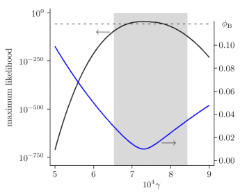
Figure 3: Boulder data: For ${0.000\rule{1.0pt}{0.0pt}5\leq\gamma\leq 0.000\rule{1.0pt}{0.0pt}9}$, the solid curve in black graphs the maximum value of $L(D|p)$ over the QM-permitted probabilities (inside the symbolic ellipse in Fig. 1); the dashed black line marks the maximum value of $L(D|p)$ over the LHV-permitted probabilities (inside the symbolic triangle in Fig. 1); and the solid curve in blue is the graph of the Bhattacharyya angle $\phi_{\mathrm{B}}^{\ }$ between the $p^{(S)}_{\alpha\beta}$s of the target state and those of the QM-MLE.

The blue curve in Fig. 3 shows the Bhattacharyya angle $\phi_{\mathrm{B}}^{\ }$ between the $p^{(S)}_{\alpha\beta}$s of the target state and those of the QM-MLE. It acquires values between $0.010\rule{1.0pt}{0.0pt}0$ for $\gamma=0.000\rule{1.0pt}{0.0pt}73$ and $0.098\rule{1.0pt}{0.0pt}9$ for $\gamma=0.000\rule{1.0pt}{0.0pt}5$. By itself, this does not provide a reliable estimate for $\gamma$ but it is consistent with, and so supports, our conclusion that $\gamma=0.000\rule{1.0pt}{0.0pt}722$ is a value with much better justification than $\gamma=0.000\rule{1.0pt}{0.0pt}5$.

The graph of the maximum likelihood as a function of $\gamma$ in Fig. 3 shows a broad maximum. This implies that values close to $\gamma=0.000\rule{1.0pt}{0.0pt}722$ can be chosen just as well. Indeed, our conclusions are unchanged if slightly different $\gamma$ values are used. Should it be necessary, for another application, to make a quantitative statement about the precision with which we infer the value of $\gamma$ from the data in Table 2, one could determine the smallest credible intervals, among them the interval of plausible values, with the methods described in Ref. Li+3:16 . This is, however, not worth the trouble in the present context.

VI.1.2 Sampling error

In Sec. V, we mentioned that there are unavoidable sampling errors. As the primary consequence, the prior contents of the three regions listed in Table 3 are uncertain. Let us see to which extent.

In the QM sampling of Sec. V.1, the next $p$ has a probability $a$ of belonging to the “QM only” region and a probability ${1-a}$ for the “both” region. The likelihood of getting a sample with $n_{1}$ $p$s in the “QM only” region and $n_{2}$ $p$s in the “both” region is

$$L^{(\mathrm{QM})}_{\mathrm{spl}}(n_{1},n_{2}|a) = \frac{(n_{1}+n_{2})!}{n_{1}!\;n_{2}!}a^{n_{1}}(1-a)^{n_{2}}$$ (39)

$$\leq L^{(\mathrm{QM})}_{\mathrm{spl}}(n_{1},n_{2}|\hat{a})$$

which is largest for $\hat{a}=n_{1}/(n_{1}+n_{2})$. Analogously, the LHV sampling of Sec. V.2 yields a sample with $n_{3}$ $p$s in the “LHV only” region and $n_{4}$ $p$s in the “both” region with a likelihood of

$$L^{(\mathrm{LHV})}_{\mathrm{spl}}(n_{3},n_{4}|b) = \frac{(n_{3}+n_{4})!}{n_{3}!\;n_{4}!}b^{n_{3}}(1-b)^{n_{4}}$$ (40)

$$\leq L^{(\mathrm{LHV})}_{\mathrm{spl}}(n_{3},n_{4}|\hat{b})$$

where $b$ is the probability that the next $p$ belongs to the “LHV only” region, and $\hat{b}=n_{3}/(n_{3}+n_{4})$ is the maximum-likelihood estimator for $b$.

Our best guesses, then, for the prior contents of the three regions are

$$S_{\mathrm{QM\,only}}^{\ }=\tfrac{1}{2}\hat{a}\,,\quad S_{\mathrm{LHV\,only}}^{\ }=\tfrac{1}{2}\hat{b}\,,$$

$$S_{\mathrm{both}}^{\ }=1-\tfrac{1}{2}(\hat{a}+\hat{b})\,,$$ (41)

since the two subsamples are of equal size, $n_{1}+n_{2}=n_{3}+n_{4}=10^{6}$. Specifically, the sample for $\gamma=0.000\rule{1.0pt}{0.0pt}722$ has $n_{1}=1\rule{1.0pt}{0.0pt}210$ and $n_{3}=993\rule{1.0pt}{0.0pt}805$, so that $\hat{a}=0.001\rule{1.0pt}{0.0pt}210$ and $\hat{b}=0.993\rule{1.0pt}{0.0pt}805$ with corresponding entries in Table 3.

With flat priors on $a$ and $b$, which are the quantities we need to infer from the sampling frequencies, we have the posterior element

$$\mathrm{d}a\,w^{(\mathrm{QM})}_{n_{1},n_{2}}(a) = \mathrm{d}a\,\frac{(n_{1}+n_{2}+1)!}{n_{1}!\;n_{2}!}a^{n_{1}}(1-a)^{n_{2}}$$ (42)

$$= \mathrm{d}a\,w^{(\mathrm{QM})}_{n_{1},n_{2}}(\hat{a})\Bigl{(}\frac{a}{\hat{a}}\Bigr{)}^{n_{1}}\Bigl{(}\frac{1-a}{1-\hat{a}}\Bigr{)}^{n_{2}}$$

$$\simeq \mathrm{d}a\,w^{(\mathrm{QM})}_{n_{1},n_{2}}(\hat{a})\,\mathrm{e}^{\mbox{\footnotesize$-\frac{1}{2}\frac{(a-\hat{a})^{2}}{v_{a}}$}}$$

for $a$ with the variance

$$v_{a}=\frac{\hat{a}(1-\hat{a})}{n_{1}+n_{2}}=\frac{n_{1}\,n_{2}}{(n_{1}+n_{2})^{3}}\,,$$ (43)

and analogous expressions for $\mathrm{d}b\,w^{(\mathrm{LHV})}_{n_{3},n_{4}}(b)$ and $v_{b}$. Accordingly, the usual one-standard-deviation confidence intervals for $a$ and $b$ are ${\hat{a}-\sqrt{v_{a}}<a<\hat{a}+\sqrt{v_{a}}}$ and ${\hat{b}-\sqrt{v_{b}}<b<\hat{b}+\sqrt{v_{b}}}$, respectively.

More in the spirit of Bayesian inference than such confidence intervals, and rather more conservative, is the plausible interval plausible which consists of all values for which

$$L^{(\mathrm{QM})}_{\mathrm{spl}}(n_{1},n_{2}|a)\geq\int\limits_{0}^{1}\mathrm{d}a^{\prime}\,L^{(\mathrm{QM})}_{\mathrm{spl}}(n_{1},n_{2}|a^{\prime})=\frac{1}{n_{1}+n_{2}+1}$$ (44)

and analogously for $b$. These intervals are

$$0.001\rule{1.0pt}{0.0pt}066<a<0.001\rule{1.0pt}{0.0pt}367\,,$$ (45)

$$0.993\rule{1.0pt}{0.0pt}475<b<0.994\rule{1.0pt}{0.0pt}124\,.$$

We thus arrive at

$$0.000\rule{1.0pt}{0.0pt}533<0.000\rule{1.0pt}{0.0pt}588<S_{\mathrm{QM\,only}}^{\ }$$

$$\hphantom{0.000\rule{1.0pt}{0.0pt}533<0.000\rule{1.0pt}{0.0pt}593}<0.000\rule{1.0pt}{0.0pt}622<0.000\rule{1.0pt}{0.0pt}683\,,$$

$$0.496\rule{1.0pt}{0.0pt}738<0.496\rule{1.0pt}{0.0pt}863<S_{\mathrm{LHV\,only}}^{\ }$$

$$\hphantom{0.496\rule{1.0pt}{0.0pt}738<0.496\rule{1.0pt}{0.0pt}501}<0.496\rule{1.0pt}{0.0pt}942<0.497\rule{1.0pt}{0.0pt}062$$ (46)

for the one-standard-deviation intervals inside the plausible intervals. These bounds quantify the sampling errors in the prior contents for $\gamma=0.000\rule{1.0pt}{0.0pt}722$ in Table 3. Very similar statements apply to the sample for $\gamma=0.000\rule{1.0pt}{0.0pt}5$ for which $n_{1}=1\rule{1.0pt}{0.0pt}173$ and $n_{2}=993\rule{1.0pt}{0.0pt}713$.

The uncertainty of the numerical values of $S_{\mathrm{QM\,only}}$, $S_{\mathrm{both}}$, and $S_{\mathrm{LHV\,only}}$ is sufficiently small to be of no further concern. Since all of the posterior content is in the “QM only” region (for $\gamma=0.000\rule{1.0pt}{0.0pt}722$), there is no doubt that the data give strong evidence in favor of this region and against the other two.

VI.1.3 No bias in the prior

We check the sample of $p$s for a bias by the procedure described in Sec. V.3, with the main objective of ensuring that the sampling algorithm does not bias the outcome in favor of the “QM only” region. We generate ten thousand $p$s at random in each of the three regions and simulate the Boulder experiment for these mock-true sets of probabilities. The resulting data are then examined whether they give evidence in favor of one of the regions. Table 6 summarizes this bias check, for $\gamma=0.000\rule{1.0pt}{0.0pt}722$.

Table 6: Boulder data, bias check of the prior: How often we get evidence in favor of one of the three regions from simulated data for 10 000 randomly chosen sets of probabilities in each of the three regions.

mock-true number of cases with probabilities evidence in favor of region in region QM only both LHV only QM only 8 809 1 278 0 both 0 8 365 1 635 LHV only 0 145 9 855

For the $10\rule{1.0pt}{0.0pt}000$ mock-true $p$s in the “QM only” region we get evidence in favor of this region in $8\rule{1.0pt}{0.0pt}809$ cases and $1\rule{1.0pt}{0.0pt}278$ times in favor of the “both” region, but never for the “LHV only” region; there are $(8\rule{1.0pt}{0.0pt}809+1\rule{1.0pt}{0.0pt}278)-10\rule{1.0pt}{0.0pt}000=87$ instances with evidence in favor of the “QM only” region and also the “both” region. The mock-true $p$s in the “both” and the “LHV only” regions never result in evidence in favor of the “QM only” region. It follows that there is no bias in the prior toward the “QM only” region and, therefore, our finding that the actual data give strong evidence in favor of this region, and against the other two, cannot be attributed to a bias in the prior.

One can read Table 6 as stating the (approximate) probabilities of finding evidence for one region, conditioned on the true $p$ being from the same or another region. It is tempting to invoke Bayes’s theorem and convert this into the probability that the true $p$ is in a certain region, given that we have evidence in favor of one of the regions. We resist this temptation because a correct application of Bayesian inference requires correctly assigned prior probabilities, which we consciously choose not to have correct-Bayes .

Table 7: Boulder data: Recorded counts in the runs one trigger signal per trial (top) for ${N=175\rule{1.0pt}{0.0pt}647\rule{1.0pt}{0.0pt}100}$ trigger signals (top); with three trigger signals per trial, for ${N=527\rule{1.0pt}{0.0pt}164\rule{1.0pt}{0.0pt}272}$ trigger signals (middle); and with seven trigger signals per trial, for ${N=1\rule{1.0pt}{0.0pt}244\rule{1.0pt}{0.0pt}205\rule{1.0pt}{0.0pt}032}$ trigger signals (bottom) Boulder-data .

$S$ $n_{++}^{(S)}$ $n_{+0}^{(S)}$ $n_{0+}^{(S)}$ $n_{00}^{(S)}$ $ab$ 1 257 629 600 43 917 556 $ab^{\prime}$ 1 417 554 4 549 43 908 718 $a^{\prime}b$ 1 281 4 341 554 43 899 021 $a^{\prime}b^{\prime}$ 11 5 640 6 030 43 894 942 $ab$ 3 800 1 936 1 812 131 804 979 $ab^{\prime}$ 4 091 1 682 13 781 131 777 583 $a^{\prime}b$ 3 853 12 840 1 669 131 749 135 $a^{\prime}b^{\prime}$ 60 16 614 17 934 131 752 503 $ab$ 8 820 4 640 4 433 311 074 665 $ab^{\prime}$ 9 512 3 963 32 709 310 997 997 $a^{\prime}b$ 9 237 30 040 4 037 310 933 331 $a^{\prime}b^{\prime}$ 159 38 632 42 034 311 010 823

VI.2 Trials with one, three, or seven trigger signals

The event counts in the runs of the Boulder experiment with one, three, or seven trigger signals per trial are given in Table 7. In total they have ${N=175\rule{1.0pt}{0.0pt}647\rule{1.0pt}{0.0pt}100}$, ${N=527\rule{1.0pt}{0.0pt}164\rule{1.0pt}{0.0pt}272}$, and ${N=1\rule{1.0pt}{0.0pt}244\rule{1.0pt}{0.0pt}205\rule{1.0pt}{0.0pt}032}$ events, respectively. Table 8 reports the prior and posterior contents of the three regions, and the data of the corresponding bias checks are given in Table 9.

Table 8: Boulder data: Prior and posterior contents of the three regions for the experimental data of Table 7; for $\gamma=0.000\rule{1.0pt}{0.0pt}722$.

  one trigger   three triggers   seven triggers   per trial   per trial   per trial region prior post. prior post. prior post. QM only 0.000 6 1 0.000 6 1 0.000 6 1 both 0.502 5 0 0.502 5 0 0.502 5 0 LHV only 0.497 0 0 0.496 9 0 0.496 9 0

Table 9: Boulder data: The analog of Table 6 for the data of Table 7. Bias checks for the runs with one (top), three (middle), and seven (bottom) trigger signals per trial; for $\gamma=0.000\rule{1.0pt}{0.0pt}722$.

mock-true number of cases with probabilities evidence in favor of region in region QM only both LHV only QM only 9 106 1 239 0 both 0 8 478 1 522 LHV only 0 85 9 915 QM only 8 898 1 229 0 both 2 8 384 1 614 LHV only 0 129 9 871 QM only 8 808 1 249 0 both 0 8 344 1 656 LHV only 0 83 9 917

The analysis of the data from these three runs confirms the conclusion of Sec. VI.1: While there is no bias in the prior toward the “QM only” region, all of the posterior is in this region; therefore, each run by itself provides strong evidence in favor of the “QM only” region and against the other two. Recall, however, what we noted at the beginning of Sec. VI, namely that the four different runs of the Boulder experiment do not use independently recorded raw data.

VII The other three experiments

VII.1 The Vienna experiment

With reference to the parameters in Table 1, we recall that the Vienna experiment is similar to the Boulder experiment, with a larger number of trigger signals and a larger nominal value of $\gamma$ while the other parameters have about the same values. The datasets numbered 6, 7, and 8 are available for evaluation Vienna-data ; see Table 10.

Mindful of the lesson learned about the crucial importance of the value of $\gamma$, we estimate its value from the data by the QSE procedure described in Sec. VI.1.1. The result of maximizing $L(D|p)$ over the QM-permissible or the LHV-permissible sets of probabilities are reported in Fig. 4(a) for the relevant range of $\gamma$ values, the analog of Fig. 3 for the Boulder data. We observe that there is not one common best-guess value for $\gamma$, as is the case for the Boulder experiment, but we have three different optimal $\gamma$ values for the three Vienna datasets, namely $\gamma_{6}=0.002\rule{1.0pt}{0.0pt}96$ for dataset 6, $\gamma_{7}=0.002\rule{1.0pt}{0.0pt}87$ for dataset 7, and $\gamma_{8}=0.002\rule{1.0pt}{0.0pt}64$ for dataset 8. The value of $\gamma=0.003\rule{1.0pt}{0.0pt}5$ in Table 1 is not an option; it is also outside the ranges of $\gamma$ values where the probabilities of the QM-MLE violate a Bell inequality of the Eberhard kind. The maximum values of the likelihood compiled in Table 11 demonstrate the case: For these best-guess values of $\gamma$ the observed data are much more likely for QM than for LHV, by many orders of magnitude. If we were to take $\gamma=0.003\rule{1.0pt}{0.0pt}5$ seriously, the data would be much much more likely for LHV than for QM, by more than 1 100 orders of magnitude for dataset 6, and more than 12 700 for dataset 8.

Table 10: Vienna data: Recorded counts in dataset 6 (top), dataset 7 (middle), and dataset 8 (bottom), with ${N=3\rule{1.0pt}{0.0pt}843\rule{1.0pt}{0.0pt}698\rule{1.0pt}{0.0pt}536}$, ${N=3\rule{1.0pt}{0.0pt}502\rule{1.0pt}{0.0pt}784\rule{1.0pt}{0.0pt}150}$, and ${N=9\rule{1.0pt}{0.0pt}994\rule{1.0pt}{0.0pt}696\rule{1.0pt}{0.0pt}192}$ trigger signals, respectively Vienna-data .

$S$ $n_{++}^{(S)}$ $n_{+0}^{(S)}$ $n_{0+}^{(S)}$ $n_{00}^{(S)}$ $ab$ 159 976 83 743 86 270 960 597 110 $ab^{\prime}$ 166 265 78 407 370 252 960 099 455 $a^{\prime}b$ 179 813 482 787 66 435 960 381 485 $a^{\prime}b^{\prime}$ 9 354 655 290 525 368 959 756 526 $ab$ 141 439 73 391 76 224 875 392 736 $ab^{\prime}$ 146 831 67 941 326 768 874 976 534 $a^{\prime}b$ 158 338 425 067 58 742 875 239 860 $a^{\prime}b^{\prime}$ 8 392 576 445 463 985 874 651 457 $ab$ 377 000 192 092 202 207 2 497 825 793 $ab^{\prime}$ 387 481 182 789 858 681 2 496 663 605 $a^{\prime}b$ 422 674 1 119 219 156 022 2 497 626 620 $a^{\prime}b^{\prime}$ 22 502 1 519 578 1 223 007 2 495 916 922

What is said in Sec. VI.1.1 is equally fitting here: (i) The computation of p-values for the purpose of refuting the LHV hypothesis does not require an accurate value of $\gamma$, but our Bayesian analysis needs an accurate value for the QM probabilities. (ii) When considered from the QM perspective, the actually observed data are not typical at all for $\gamma=0.003\rule{1.0pt}{0.0pt}5$.

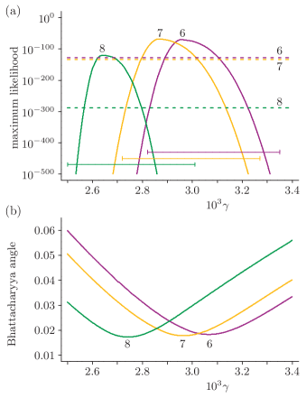
Figure 4: Vienna data: (a) For ${0.002\rule{1.0pt}{0.0pt}5\leq\gamma\leq 0.003\rule{1.0pt}{0.0pt}4}$, the solid curves graph the maximum values of $L(D|p)$ over the QM-permitted probabilities (inside the symbolic ellipse in Fig. 1) for dataset 6 (purple), dataset 7 (orange), and dataset 8 (green); the dashed lines mark the corresponding maximum values of $L(D|p)$ over the LHV-permitted probabilities (inside the symbolic triangle in Fig. 1). The values for $\gamma=0.003\rule{1.0pt}{0.0pt}5$ are far outside the range of the plot: $3.9\times 10^{-1286}$ for dataset 6, $5.5\times 10^{-1875}$ for dataset 7, and $2.8\times 10^{-13060}$ for dataset 8; see also Table 11. The horizontal bars show the respective ranges of $\gamma$ values for which the probabilities of the QM-MLE violate a Bell inequality of the Eberhard kind; these ranges correspond to the grey strip in Fig. 3.
(b) For the same $\gamma$ range, the curves graph the Bhattacharyya angle between the $p_{\alpha\beta}^{(S)}$s of the target state and those of the QM-MLE. The angle is smallest for ${\gamma=0.003\rule{1.0pt}{0.0pt}07}$, $0.002\rule{1.0pt}{0.0pt}96$, and $0.002\,74$ for dataset 6, dataset 7, and dataset 8, respectively.

In Fig. 4(b) we show the Bhattacharyya angle $\phi_{\mathrm{B}}^{\ }$ between the probabilities of the target state and those of the QM-MLE. Analogous remarks to those about Fig. 3 apply here as well: The angle is small for the $\gamma$ values for which the corresponding QM likelihood is large, and this supports our conclusion that $\gamma_{6}=0.002\rule{1.0pt}{0.0pt}96$, $\gamma_{7}=0.002\rule{1.0pt}{0.0pt}87$, and $\gamma_{8}=0.002\rule{1.0pt}{0.0pt}64$ are values with much better justification than $\gamma=0.003\rule{1.0pt}{0.0pt}5$.

Table 11: Vienna data: Maximum values of the likelihood $L(D|p)$ for QM-permissible probabilities with selected values of $\gamma$, and for LHV-permissible probabilities.

$\gamma$ dataset 6 dataset 7 dataset 8 $0.002\rule{1.0pt}{0.0pt}64$ $7.9\times 10^{-1503}$ $5.3\times 10^{-732}$ $5.1\times 10^{-121}$ $0.002\rule{1.0pt}{0.0pt}87$ $2.4\times 10^{-170}$ $8.5\times 10^{-69}$ $1.8\times 10^{-569}$ $0.002\rule{1.0pt}{0.0pt}96$ $6.3\times 10^{-71}$ $1.7\times 10^{-91}$ $3.4\times 10^{-1097}$  QM  $0.003\rule{1.0pt}{0.0pt}5\phantom{0}$ $3.9\times 10^{-1286}$ $5.5\times 10^{-1875}$ $2.8\times 10^{-13060}$ LHV, any $\gamma$ $4.7\times 10^{-129}$ $5.5\times 10^{-134}$ $3.4\times 10^{-289}$

While slightly different values for $\gamma_{6}$, $\gamma_{7}$, and $\gamma_{8}$ are equally acceptable, we emphasize that there is no common value. It appears that the intensity of the pump laser, whose pulses trigger the generation of down-converted photon pairs with entangled polarization qubits, was largest for dataset 6 and smallest for dataset 8, with correspondingly different $\gamma$ values Wengerowsky-private . We proceed under the assumption that the value of $\gamma$ was stable enough during each run that it is reasonable to apply a single effective $\gamma$ value to each of the three datasets drift .

Table 12: Vienna data: Prior and posterior contents of the three regions for the experimental data of Table 10 with the respective best-guess values for $\gamma$. As in Table 3 above and also in Table 16 below, the prior contents have sampling errors of no consequence; see Sec. VI.1.2.

data set 6 data set 7 data set 8 ${\gamma=0.002\rule{1.0pt}{0.0pt}96}$ ${\gamma=0.002\rule{1.0pt}{0.0pt}87}$ ${\gamma=0.002\rule{1.0pt}{0.0pt}64}$ region prior post. prior post. prior post. QM only 0.001 8 1 0.001 9 1 0.001 8 1 both 0.501 8 0 0.501 7 0 0.501 8 0 LHV only 0.496 4 0 0.496 4 0 0.496 4 0

When checking the datasets of the Vienna experiment for evidence in favor of or against the regions symbolized in Fig. 1, we find the prior and posterior contents of Table 12. Once more we have strong evidence in favor of the “QM only” region and against the other two. This conclusion is what the data tell us. It is not a consequence of a biased prior, as is demonstrated by the due-diligence bias check documented in Table 13 which uses ten thousand mock-true sets of probabilities for each region and each data set.

Table 13: Vienna data: The analogs of Tables 6 and 9, here for the data of Table 10. Bias checks for dataset 6 (top), dataset 7 (middle), and dataset 8 (bottom), for the respective best-guess values of $\gamma$.

mock-true number of cases with probabilities evidence in favor of region in region QM only both LHV only QM only 9 225 778 0 both 0 8 545 1 455 LHV only 0 94 9 906 QM only 9 229 775 0 both 1 8 341 1 658 LHV only 0 137 9 863 QM only 9 264 736 0 both 1 8 599 1 400 LHV only 0 82 9 918

VII.2 The Delft and Munich experiments

As a consequence of exploiting other physical systems, the parameters in Table 1 are quite different for the Delft and Munich experiments than for the Vienna and Boulder experiments. In particular, there is ${\gamma=1}$ in the Delft and Munich experiments, and no estimation of $\gamma$ is called for, and also ${\eta^{\ }_{\mathrm{A}},\eta^{\ }_{\mathrm{B}}\lesssim 1}$ are more advantageous values, whereas there are much fewer trigger signals, which is a drawback.

Table 14: Delft and Munich data: Recorded counts in run 1 (top left) and run 2 (top right) of the Delft experiment, with ${N=245}$ and ${N=228}$ trigger signals, respectively Delft-data ; and in run 1 (middle) and run 2 (bottom) of the Munich experiment, with ${N=27\rule{1.0pt}{0.0pt}885}$ and ${N=27\rule{1.0pt}{0.0pt}683}$ trigger signals, respectively Munich-data . The marked difference in the relative frequencies for ${S=a^{\prime}b}$ and ${S=a^{\prime}b^{\prime}}$ in the two runs of the Munich experiment originates in the use of two different target states.

$S$ $n_{++}^{(S)}$ $n_{+0}^{(S)}$ $n_{0+}^{(S)}$ $n_{00}^{(S)}$ $ab$ 23$|$21 3$|$7 4$|$3 23$|$21 $ab^{\prime}$ 33$|$25 11$|$20 5$|$4 30$|$23 $a^{\prime}b$ 22$|$19 10$|$11 6$|$6 24$|$23  Delft  $a^{\prime}b^{\prime}$ 4$|$5 20$|$24 21$|$23 06$|$11 $ab$ 778 2 621 2 770 804 $ab^{\prime}$ 809 2 629 2 708 816 $a^{\prime}b$ 873 2 686 2 644 730 $a^{\prime}b^{\prime}$ 2 696 966 902 2 453 $ab$ 817 2 596 2 873 742 $ab^{\prime}$ 696 2 570 2 788 772 $a^{\prime}b$ 2 783 787 840 2 503  Munich  $a^{\prime}b^{\prime}$ 865 2 620 2 640 791

The data from two runs each for the Delft and the Munich experiments are available for evaluation Delft-data ; Munich-data ; see Table 14. We begin the evaluation with a maximization of the likelihood $L(D|p)$ over the set of QM-permissible probabilities and also over the set of LHV-permissible probabilities. As the entries in Table 15 show, the observed data are much more likely for QM-permissible than for LHV-permissible probabilities, with ratios between $7.2$ and $6.5\times 10^{15}$. Since the two runs of the Delft experiment had exceptionally few events, less than one-hundredth of the counts in the Munich experiment, we also combined the data of the two Delft runs into one larger set with ${N=473}$ trigger signals (“run 1&2”), and that is included in Table 15 as well Delft-3rd . Not only is there no corresponding need to combine the data of the two runs of the Munich experiment, this would not be proper to begin with, as there were two different target states; see Table 14.

Table 15: Delft and Munich data: Maximum values of the likelihood $L(D|p)$ for QM-permissible probabilities and for LHV-permissible probabilities. The last column gives the ratios of the two maximum-likelihood values.

QM LHV ratio Delft run 1 $2.95\times 10^{-16}$ $4.10\times 10^{-17}$ $7.2$ Delft run 2 $8.20\times 10^{-15}$ $2.63\times 10^{-15}$ $3.1$ Delft run 1&2 $1.22\times 10^{-17}$ $1.04\times 10^{-18}$ $12$ Munich run 1 $2.17\times 10^{-30}$ $5.27\times 10^{-34}$ $4.1\times 10^{3}$ Munich run 2 $2.88\times 10^{-31}$ $4.46\times 10^{-47}$ $6.5\times 10^{15}$

Table 16: Delft and Munich data: Prior and posterior contents of the three regions for the experimental data of Table 14.

Delft, run 1 Delft, run 2 Delft, run 1&2 Munich, run 1 Munich, run 2 region prior posterior prior posterior prior posterior prior posterior prior posterior QM only 0.151 2 1.000 000 0.151 2 0.999 980 0.151 3 1.000 000 0.076 9 1 0.077 0 1 both 0.362 7 1.2$\times 10^{-7}$ 0.362 7 7.0$\times 10^{-6}$ 0.362 8 6.7$\times 10^{-9}$ 0.426 7 0 0.426 6 0 LHV only 0.486 0 4.5$\times 10^{-8}$ 0.486 0 1.3$\times 10^{-5}$ 0.486 0 1.6$\times 10^{-10}$ 0.496 4 0 0.496 4 0

Figure 5: Delft and Munich data: Probability-space triangles. The corners of the triangles indicate the sets of probabilities for the respective target state (circle), QM-MLE (square), and the relative frequencies observed (unmarked corner). The black triangles at the top are for runs 1, 2, and 1&2 of the Delft experiment (left to right) and the blue triangles below are for the two runs of the Munich experiment. The lengths of the sides of the triangles are the Bhattacharyya angles between the probabilities at the corners, on the indicated scale.

The Bhattacharyya angle is a genuine distance between two sets of probabilities. Therefore, the three angles between the relative frequencies, the $p^{(S)}_{\alpha\beta}$s of the target states, and those of the QM-MLE, constitute the sides of a triangle. In Fig. 5 we show the three triangles for runs 1, 2, and 1&2 of the Delft experiment at the top (in black) and the two triangles for the runs of the Munich experiment below (in blue). These are five independent drawings with no relations among them, except that the scale is the same, defined by the reference line for an angle of $0.100$. In each triangle, the circle marks the target state, the square marks the QM-MLE, and the third corner is for the relative frequencies.

As it should be, the QM-MLE is always nearer to the relative frequencies than the target state, somewhat nearer for the Delft runs, much nearer for the Munich runs. The Bhattacharyya angles between the probabilities of the target state and those of the QM-MLE for the data of the Boulder and Vienna experiments, evaluated for the respective best-guess value for $\gamma$, are markedly smaller, namely $0.011$ for the Boulder experiment, and $0.020$ for the Vienna experiment. The red-line stretches indicate these distances in Fig. 5; they are to be compared with the distances between circles and squares.

This comparison indicates that the precision with which the intended target state is realized in the Boulder and Vienna experiments is noticeably better than that in the Delft and Munich experiments, which certainly did also succeed with good precision. While this observation has no bearing on our conclusions, it does illustrate what the data tell us when putting questions to them.

For the data in Table 14 we find the prior and posterior contents of the three regions reported in Table 16, including also the combined Delft data (“run 1&2”). When comparing the prior contents in Table 16 with those in Tables 3, 8, and 12, we notice that the “QM only” region has a much larger prior content for the Delft and Munich data than for the Boulder and Vienna data.

This difference results predominantly from an increase of the “QM only” fraction and a decrease of the “both” fraction in the QM sample (see Sec. III.1). This different distribution in turn originates mainly in the larger detection efficiencies $\eta^{\ }_{\mathrm{A}}$ and $\eta^{\ }_{\mathrm{B}}$ and, to a lesser extent, also in the larger angles $\theta^{\ }_{\mathrm{A}}$ and $\theta^{\ }_{\mathrm{B}}$; see Table 1. These parameters directly enter the QM probabilities of Eqs. (III.1) and (14) but not the LHV probabilities of Eq. (III.2). Notice also that the “QM only” region for the Delft experiment has about twice the prior content of that for the Munich experiment, mostly a consequence of the imperfections mentioned in note Munich-dark . By contrast, the very substantial difference in the value of $\gamma$ is of little consequence because a change in $\gamma$ leads to an overall scaling of the regions without changing their relative size, as is most clearly seen when we look at the accessible region of just one of the four 3-simplices (recall that ${p^{(S)}_{00}\geq 1-\gamma}$).

The posterior contents for the Munich data are as extreme as we observed for the Boulder and the Vienna data: Only the “QM only” region has posterior content. Just like the data of the Boulder and Vienna experiments do, the data of the Munich experiment give very strong evidence in favor of the “QM only” region and against the other two regions.

While the data of the Delft experiment also give evidence of the same kind, the evidence is less strong than in the other experiments, simply because there are so many fewer events. Nevertheless, the evidence against LHV is strong, certainly stronger than the p-value of 0.039 suggests Delft . This p-value is below the conventional 0.05 threshold which is taken to imply evidence against; see also Benjamin+71:17 . We note, however, that even if a p-value was above any such threshold, then this could not be taken as evidence for the hypothesis in question and that is in sharp contrast to the approach we follow here.

Table 17: Delft and Munich data: The analog of Tables 6, 9, and 13, here for the bias check on the priors for the data of Table 14. One thousand mock-true $p$s are used for each region and run.

mock-true number of cases with probabilities evidence in favor of region in region QM only both LHV only QM only 971 153 0 both 65 810 216 LHV only 8 48 958 QM only 973 176 4 both 67 801 236 LHV only 5 46 961 QM only 979 124 0 both 47 852 177  Delft  run 1&2  run 2   run 1  LHV only 1 25 980 QM only 982 25 0 both 5 860 136 LHV only 0 12 988 QM only 988 22 0 both 3 865 133  Munich   run 2   run 1  LHV only 0 9 991

Here, too, the analysis would be incomplete without a confirmation that there is no bias in the prior. Table 17 shows how often we find evidence in favor of the three regions when simulating data for one-thousand mock-true $p$s from each of the regions. As discussed in Sec. V.3, the obvious difference between this Table and Tables 6, 9, and 13 originates in the smaller counts of event (Munich) or the much smaller ones (Delft). Even so, although it can happen more easily here that we find evidence in favor of the “QM only” region from data for probabilities from another region, there is no procedural bias for the “QM only” region.

VIII Discussion and conclusion

Our analysis is based entirely on the event counts in Tables 2, 7, 10, and 14, with no other information about the recorded data. Therefore, our analysis must assume that for each run of one of the four experiments, the corresponding list of counts is a sufficient statistic. In particular, this brings up the issues of notes runs-test and drift , namely that the sequences of detected events do not exhibit correlations that should not be there, so that the experiments can be reliably evaluated with the parameters in Table 1, even if we found it necessary to estimate the trigger–to–qubit-pair conversion probabilities from the data themselves (Boulder and Vienna).

Therefore, we do not worry about the so-called “memory loophole” — the notion that the LHV could keep track of past outcomes and adjust the probabilities for future ones in the most deceiving way. Nor do we entertain scenarios in which the detectors communicate with each other through unknown means (dark-matter waves perhaps?) with, again, fitting adjustments for future outcomes. Rather, we take for granted that the data have been thoroughly checked for correlations that would result from such mechanisms, and that none were found.

As explained in the Introduction, our choice of prior does not follow the rules of proper Bayesian reasoning. Our prior, defined by the sampling algorithm described in Sec. V, ignores the rules deliberately. It does not take into account any prior knowledge we have about the experimental situation — that there is strong prior evidence for QM and none at all for LHV, and that the experimenters have the skills to build the apparatus as specified. Instead, our prior leans heavily toward LHV — the prior content of the “LHV only” region is larger in all samples, sometimes much larger, than that of the “QM only” region — and that there really is no procedural bias for QM is demonstrated by our bias checks, one such test of the prior used in each experimental context. The bias checks are a priori and do not depend on the observed data.

Even with all this support extended to LHV, the data provide very strong evidence in favor of QM and against LHV. This is especially convincing in the face of the procedural advantage given to LHV.

In closing, we wish to remind the reader that nonquantum formalisms with LHV do not amount to a serious alternative to the QM description. Successful LHV accounts of any recorded data have always been limited to very particular experimental situations and relied on a case-by-case ad-hoc reasoning. The plethora of phenomena that are correctly accounted for by QM are simply beyond the reach of LHV. Yet, even within this limited context in which LHV have a slim chance of success they have been refuted for good.

IX Outlook

While the “QM vs LHV case” is at the center stage of this work, there is a more general lesson here about the use of Bayesian methods when asking what evidence is provided by empirical data. On the conceptual side, there is the Bayesian principle of evidence: We have evidence in favor of an alternative if it is more probable after the data are available than before; and there is evidence against the alternative if the data render it less probable. On the procedural side, there is the systematic checking of the chosen prior for an unwanted bias in order to ensure that the conclusions are not predetermined.

This approach is applicable to many situations. Let us mention just one. Suppose you have a source of qutrit pairs and you want to verify that it prepares the pairs in a state with bound entanglement Sentis+4:18 . You could then collect tomographic data and determine whether there is evidence in favor of the set of bound-entangled states, or against it.

- (1) B. Hensen, H. Bernien, A. E. Dréau, and 16 co-authors, Loophole-free Bell inequality violation using electron spins separated by 1.3 kilometers, Nature (London)526, 682 (2015).
- (2) M. Giustina, M. A. M. Versteegh, S. Wengerowsky, and 19 co-authors, Significant-Loophole-Free Test of Bell’s Theorem with Entangled Photons, Phys. Rev. Lett. 115, 250401 (2015).
- (3) L. K. Shalm, E. Meyer-Scott, B. G. Christensen, and 31 co-authors, Strong Loophole-Free Test of Local Realism, Phys. Rev. Lett. 115, 250402 (2015).
- (4) W. Rosenfeld, D. Burchardt, R. Garthoff, K. Redeker, N. Ortegel, M. Rau, and H. Weinfurter, Event-Ready Bell Test Using Entangled Atoms Simultaneously Closing Detection and Locality Loopholes, Phys. Rev. Lett. 119, 010402 (2017).
- (5) J. Bell, On the Einstein–Podolsky–Rosen paradox, Physics 1, 195 (1964).
- (6) J. F. Clauser, M. A. Horne, A. Shimony, and R. A. Holt, Proposed Experiment to Test Local Hidden-Variable Theories, Phys. Rev. Lett. 23, 880 (1969); ibid. 24, 549 (1970).
- (7) P. H. Eberhard, Background level and counter efficiencies required for a loophole-free Einstein–Podolsky–Rosen experiment, Phys. Rev. A47, R747 (1993).
- (8) See, for example, Sec. 3.4 in Ref. Evans:15 .
- (9) R. L. Wasserstein and N. A. Lazar, The ASA’s Statement on p-Values: Context, Process, and Purpose, The American Statistician 70, 129 (2016).
- (10) D. J. Benjamin, J. O. Berger, M. Johannesson, and 69 co-authors, Redefine statistical significance, Nature Human Behaviour 2, 6 (2017).
- (11) M. Evans, Measuring Statistical Evidence Using Relative Belief, Monographs on Statistics and Applied Probability, vol. 144 (CRC Press, Taylor & Francis Group, 2015).
- (12) See Chapter 4 in Ref. Evans:15 . We note that it is customary to measure the strength of evidence by the size of the so-called “Bayes factor” but this practice is questionable in view of the Jeffreys–Lindley paradox Jeffreys:39 ; Lindley:57 and other deficiencies.
- (13) G. Boole, On the Theory of Probabilities, Phil. Trans. R. Soc. London 152, 225 (1862).
- (14) Here, we only evaluate the data on which Refs. Delft ; Vienna ; Boulder ; Munich are based; for some runs, we got access to data that were not as such published in these references or their supplemental material through private communications with the experimental teams. This help is gratefully acknowledged. We are not evaluating the data from other, earlier Bell-test experiments, nor data from later experiments, except for the second run of the Delft experiment Delft-2nd .
- (15) B. Hensen, N. Kalb, M. S. Blok, and 11 co-authors, Loophole-free Bell test using electron spins in diamond: second experiment and additional analysis, Sci. Rep. 6, 30289 (2016).
- (16) In the detection stage of the Munich experiment, atoms are ionized, and the ions and electrons are detected separately, with efficiencies of for the ion detection and for the electron detection. Since detection is successful if either an ion or an electron or both are found, this results in an overall detection efficiency between 0.975 and 0.994. The lower limit is displayed in Table 1 and used for the data evaluation reported in Sec. VII.2; other values could be used for and equally well, with no change in our final conclusions.
- (17) In the Munich experiment, 98% of the atoms with pass the selector and also 4% of the atoms with , and likewise for , , and (private communication with K. Redeker and W. Rosenfeld; see also Refs. Henkel:11 ; Ortegel:16 ; Krug:18 ). This matter is taken into account in Sec. VII.2.
- (18) N. Brunner, D. Cavalcanti, S. Pironio, V. Scarani, and S. Wehner, Bell nonlocality, Rev. Mod. Phys. 86, 419 (2014).
- (19) E. P. Wigner, On Hidden Variables and Quantum Mechanical Probabilities, Am. J. Phys. 38, 1005 (1970).
- (20) A. Fine, Joint distributions, quantum correlations, and commuting observables, J. Math. Phys. 23, 1306 (1982).
- (21) D. Kaszlikowski, P. Gnaciński, M. Żukowski, W. Miklaszweski, and A. Zeilinger, Violations of Local Realism by Two Entangled -Dimensional systems Are Stronger than for Two Qubits, Phys. Rev. Lett. 85, 4418 (2000).
- (22) We trust that runs tests have confirmed this statistical independence. We cannot perform runs tests ourselves on all data sets as we do not know the sequence of detection events for some of them. For all experiments evaluated, we only explore the total counts of recorded detection events (Tables 2, 7, 10, and 14), not the order in which they were recorded. The list of counts is a sufficient statistic if the events are statistically independent, and only then.
- (23) M. Froissard, Constructive generalization of Bell’s inequalities, Nuovo Cimento B 64, 241 (1981).
- (24) Y.-L. Seah, J. Shang, H. K. Ng, D. J. Nott, and B.-G. Englert, Monte Carlo sampling from the quantum state space. II, New J. Phys. 17, 043018 (2015).
- (25) See Table S-II in the Supplemental Material to Ref. Boulder .
- (26) M. Paris and J. Řeháček, eds., Quantum State Estimation, Lect. Notes Phys. 649 (2004).
- (27) J. Shang, H. K. Ng, A. Sehrawat, X. Li, and B.-G. Englert, Optimal error regions for quantum state estimation, New J. Phys. 15, 123026 (2013).
- (28) Y. S. Teo, Introduction to quantum-state estimation (World Scientific, Singapore, 2016).
- (29) J. Shang, Z. Zhang, and H. K. Ng, Superfast maximum likelihood reconstruction for quantum tomography, Phys. Rev. A95, 062338 (2017).
- (30) R. J. Adler, B. Casey, and O. C. Jacob, Vacuum catastrophe: An elementary exposition of the cosmological constant problem, Am. J. Phys. 63, 620 (1995).
- (31) D. Mogilevtsev, Calibration of single-photon detectors using quantum statistics, Phys. Rev. A82, 021807 (2010).
- (32) A. M. Braczyk, D. H. Mahler, L. A. Rozema, A. Darabi, A. M. Steinberg, and D. F. V. James, Self-calibrating quantum state tomography, New J. Phys. 14, 085003 (2012).
- (33) N. Quesada, A. M. Brańczyk, and D. F. V. James, Self-calibrating tomography for multidimensional systems, Phys. Rev. A87, 062118 (2013).
- (34) The no-signaling conditions of Eqs. (III) and (III) matter. If we maximize by only imposing the four constraints of Eq. (9), we obtain , more than seven times the value with the no-signaling conditions enforced.
- (35) A. Bhattacharyya, On a measure of divergence between two statistical populations defined by their probability distributions, Bull. Calcutta Math. Soc. 35, 99 (1943).
- (36) The observation that the given value is incorrect is an example of model checking and by itself not part of the Bayesian data analysis. For , the QM model is in conflict with the data — the data are so highly untypical that the model is wrong. By switching from to we arrive at a correct model. An analogous statement applies to the Vienna experiment in Sec. VII.1.
- (37) X. Li, J. Shang, H. K. Ng, and B.-G. Englert, Optimal error intervals for properties of the quantum state, Phys. Rev. A94, 062112 (2016).
- (38) See Sec. 4.5.2 in Evans:15 and Sec. VI in Li+3:16 .
- (39) By a correct application of Bayesian inference we mean the use of a prior that fully reflects our strong beliefs concerning the truth of QM and we have purposefully not done that here but rather chose to be much more even-handed.
- (40) The data of the Boulder experiment are retrieved from L. K. Shalm and S. W. Nam, Data for “Strong loophole-free test of local realism” (National Institute of Standards and Technology, DOI: 10.5060/D2JW8BTT, 2015) at https://www.nist.gov/pml/applied-physics-division/repository-bell%-te!st-research-software-and-data.
- (41) Dataset 7 of the Vienna experiment is retrieved from M. Giustina, Bell’s inequality and two conscientious experiments (Dissertation, Universität Wien, 2016) at https://ubdata.univie.ac.at/AC13728804. Datasets 6 and 8 are from private communication with S. Wengerowsky; we thank for the permission to report these data here.
- (42) S. Wengerowsky, private communication (2018).
- (43) A remark similar to that in note runs-test applies: We cannot test this assumption on the basis of the data in Table 10 as one would need to compare the data recorded at different intervals of the data-taking period. We trust that the data have been tested for drifts in the experimental parameters and none were found within each of the three datasets.
- (44) The data of the Delft experiment are retrieved from https://data.4tu.nl/repository/uuid:6e19e9b2-4a2!d-40b5-8dd3-a660bf3c0a31 (run 1) and https://data.4tu.nl/repository/uuid:53644d31-d862-4f9f-9ad2-!0b571874b829 (run 2).
- (45) The data of the Munich experiment are retrieved from the supplemental material to Ref. Munich at http://link.aps.org/supplemental/10.1103/PhysRevLett.119.010402.
- (46) There is also a “third run” of the Delft experiment with a different target state as run 1 and run 2 and a total of trigger signals Delft-2nd . We do not include these data in our analysis.
- (47) G. Sentís, J. N. Greiner, J. Shang, J. Siewert, and M. Kleinmann, Bound entangled states fit for robust experimental verification, eprint arXiv:1804.07562 [quant-ph] (2018).
- (48) H. Jeffreys, Theory of Probability (Oxford University Press, 1939).
- (49) D. V. Lindley, A Statistical Paradox, Biometrika 44, 187 (1957).
- (50) F. Henkel, Photoionisation detection of single -atoms using channel electron multipliers, Ph.D. thesis (University of Munich, 2011).
- (51) N. Ortegel, State readout of single Rubidium-87 atoms for a loophole-free test of Bell’s inequality, Ph.D. thesis (University of Munich, 2016).
- (52) M. Krug, Ionization Based State Read Out of a single Atom, Ph.D. thesis (University of Munich, 2018).