Route to chaos in a coupled microresonator system with gain and loss

Abstract

We consider chaotic dynamics of a system of two coupled ring resonators with a linear gain and a nonlinear absorption. Such a structure can be implemented in various settings including microresonator nanostructures, polariton condensates, optical waveguides or atomic Bose-Einstein condensates of ultra-cold atoms placed in a circular-shaped trap. From the theoretical point of view this system is attractive due to its modulational instability and rich structure, including various types of spontaneous symmetry breaking, period doubling bifurcations, eventually leading to chaotic regime. It is described by set of partial differential equations but we show that the so called Galerkin approximation can explain most of the system characteristics mapping it on the dynamics of few coupled oscillator modes. The main goal of present study is to investigate various routes to chaos in our non-hermitian system and to show the correspondence between the continuous operator problem and its discrete representation.

1 Introduction

While it is quite common to consider physical models with a linear loss, fibre optics serves as one of the areas where nonlinear loss phenomena, due to stimulated Brillouin or Raman scattering Smith72 ; Agra01 ; Boyd play an important role. These effects are effectively described by Kerr-like (cubic) nonlinearities. Moreover, this nonlinearity bridges the two seemingly remote areas of physics such as the nonlinear optics and cold atom physics. It was revealed about 20 years ago, while considering wave mixing in atomic condensates 4WM ; atomlaser . For atomic condensate the loss may be due to two or three body inelastic interactions. Note also that strong nonlinear loss is present in Bose-Einstein condensate (BEC) of exciton polaritons in a semiconductor microcavity dakis ; newbook , which is a macroscopically populated coherent quantum state subject to concurrent pumping and decay.

On that account the model that we propose to study here can be applied to both BECs of exciton polaritons and to optical nanostructures of coupled microresonators. One and the other belong to the rapidly developing fields of both theoretical and experimental physics, receiving lately a lot of attention. The former consists of bosonic quasi-particles that exist inside semiconductor microcavities, in the form of a superposition of an exciton and a cavity photon and exhibit a transition to quantum degeneracy akin to (BEC) EPC1 ; EPC2 ; EPC3 ; EPC4 ; EPC5 . The latter holds the possibility to create a new platform for biological sensing applications plat . Optical microresonators were also investigated in the context of switches switches1 ; switches2 , lasers, lasers1 ; lasers2 ; lasers3 , temporal solitons optsol1 ; optsol2 ; optsol3 ; optsol4 , soliton frequency combs freqcomb1 ; freqcomb2 ; freqcomb3 , and even a transition to chaos michaos .

In the following we shall consider a particular example of such a system - a two coupled rings structure. This geometry has numerous interesting features from both, theoretical (periodic boundary conditions, indicating mode quantization) and experimental (easy fabrication in nano-structured systems, potential applications) perspectives.

The model is presented in Sec. 2. It was studied by some of us earlier revealing rich dynamical behavior such as the spontaneous symmetry breaking, modulational instability or complex and persistent flow of currents between the rings SciRep ; Symmetry . In the present work we concentrate on the route of chaos, which may be observed in this system as demonstrated numerically in Sec. 3.

Previously we demonstrated that in the regime of regular motion the system is well described by an analytic few mode Galerkin approximation (GA) Ern originally proposed for solving of the Laplace equation in the electric field galerkin . In mathematics, in the area of numerical analysis, Galerkin methods are a class of methods for converting a continuous operator problem (such as a differential equation) to a discrete problem. It uses a linear combination of basis functions with weights determined by minimizing a globally integrated measure of the error in the solution. It is widely used in the analysis of various scientific and engineer problems (see for example Chekroun ; Wanga ) including models described by the Gross-Pitaevskii equation (GPE) with harmonic oscillator potential GA-Malomed or in multi-component space Driben16 ; Wang17 . There is a broad spectrum of GA applications in descriptions of physical and chemical processes, where statistical models are used apps1 ; apps2 and the Galerkin expansion allows to significantly simplify the problem. Here we prove that this approach can also help to understand the chaotic instability of our system, and when appropriate number of modes is included, is practically indistinguishable from the continuous model.

2 The model

We consider two coupled rings structure. Apart from a cubic nonlinearity, we assume that the system is interacting with the environment. This interaction is characterized by the presence of a linear gain and nonlinear losses. We adopt the mean field model SciRep described by a pair of Gross-Pitaevskii equations (GPE) coupled by a linear homogeneous term, characterized by a constant coupling $c$

$$i\frac{\partial\Psi_{1}}{\partial t}=-\frac{\partial^{2}\Psi_{1}}{\partial x^{2}}+i\gamma\Psi_{1}+\left(1-i\Gamma\right)|\Psi_{1}|^{2}\Psi_{1}+c\Psi_{2}$$

$$i\frac{\partial\Psi_{2}}{\partial t}=-\frac{\partial^{2}\Psi_{2}}{\partial x^{2}}+i\gamma\Psi_{2}+\left(1-i\Gamma\right)|\Psi_{2}|^{2}\Psi_{2}+c\Psi_{1}.$$ (1)

Here the term with $\gamma$ is responsible for a linear gain, while that with $\Gamma$ quantifies nonlinear losses (all parameters are assumed to be homogeneous across the whole structure). We choose the units in such a way that interactions within each ring lead to a Kerr-like nonlinearity of unit strength. The assumed geometry implies that $x\in\left\langle 0,2\pi\right)$ is an angular variable and periodic boundary conditions are applied, i.e. $\Psi_{i}\left(x,t\right)=\Psi_{i}\left(x+2\pi,t\right)$. Due to these boundary conditions the system reveals an apparent quantization with only discrete modes being allowed for the dynamics. Note that the same set of equations (1) describes a single ring with a spinor (spin=1/2) condensate with spin components coupled by $c$-proportional term, but also the exciton-polariton systems in the microcavities and even nano-photonics systems nano . The system (1) appears also as a simplified model with a quintic nonlinearity and diffusion introduced and studied numerically subject to zero boundary conditions in Malomed .

The system described by Eq. (1) reveals very rich dynamics SciRep and is very sensitive to both the change of the initial conditions and the particular values of parameters, in particular, to the value of the coupling between rings, denoted by $c$. One may find different (symmetric and antisymmetric) solutions of (1), as it is discussed at lengths in our previous study SciRep . Interestingly stationary inhomogeneous states also exist - they manifest spontaneous translational symmetry breaking. Following SciRep let us denote by $\kappa$ the following integral

$$\kappa=\frac{1}{2\pi}\int_{0}^{2\pi}\frac{\partial}{\partial x}{\mathrm{a}rg}(\Psi_{i})dx.$$ (2)

Due to the ring quantization $\kappa$ takes integer values only and will be referred to as a topological charge in the spirit of a vortex terminology.

One can check that during the time evolution the topological charge does not have to be conserved, so it is relatively easy to observe stable vortices. Indeed our coupled system permits solutions of the form (out-of-phase)

$$\Psi_{1}(x,t)=-\Psi_{2}(x,t)=\sqrt{\frac{\gamma}{\Gamma}}e^{i\left[\kappa x-(\frac{\gamma}{\Gamma}+\kappa^{2}-c)t\right]}$$ (3)

which are stable for the whole range of parameters $\Gamma,\gamma$ and $c$, in analogy with antisymmetric solutions. There exists also in-phase solutions

$$\Psi_{1}(x,t)=\Psi_{2}(x,t)=\sqrt{\frac{\gamma}{\Gamma}}e^{i\left[\kappa x-(\frac{\gamma}{\Gamma}+\kappa^{2}+c)t\right]}.$$ (4)

All modes mentioned above are stable for specific ranges of parameters and in SciRep we constructed a two dimensional map in $\gamma/\Gamma$ and $c$ to characterize the spectrum of stable solutions. In SciRep we also discussed stability condition, applying linear stability analysis. In the present study we focus on possible instabilities describing in detail the ”route to chaos” scenarios. The results are presented in the next section, followed by an approximate analysis based on the Galerkin approximation.

3 Route to chaos

We consider the evolution described by Eq. (1) for given values of control parameters: the gain $\gamma$, the loss $\Gamma$ and the coupling between rings, $c$. To address the issue of a transition from a regular to a chaotic behavior we sample the dynamics in various configurations. First we keep the gain and loss parameters at constant values ($\Gamma=1$ and $\gamma=1.75$) and we compare the solutions for different values of the coupling $c$. Then we keep $c$ and $\gamma$ fixed and vary $\Gamma$, and finally we present two dimensional $c-\gamma$ map for $\Gamma=1$. In each case we start from the same kind of the initial conditions, slightly perturbed unstable, symmetric, stationary state

$$\Psi_{1,2}\left(x,0\right)=\sqrt{\frac{\gamma}{\Gamma}}\left[1\pm\sum_{k=1}^{l}A^{k}_{0}cos\left(kx\right)\right],$$ (5)

with upper and lower signs corresponding to the first and second ring, respectively. The small perturbation amplitude is equal to $A^{k}_{0}=10^{-2}$ for all $k$. Notice that due to periodic boundary conditions we have a discrete spectrum of available spatial modes $k$. For a regular regime, a choice of $A_{0}^{k}$ seems not important. We have checked that long time evolution is not affected by the choice of an initial perturbation. However, as we shall see on the example below even a small modification of the initial conditions affects the long time solution obtained in the ”chaotic” regime.

We have observed that asymptotically, for each set of control parameters, there is a clear behavior that can be classified within the limited set of categories: an antisymmetric state, a vortex state (as defined above), a limit cycle (with one or more frequencies), or finally, an irregular motion that reveals the features of the chaotic dynamics. In the previous study SciRep we presented in a compact way the whole gallery of these states in some range of parameters. Here we focus on a small range of states to show possible ”routes to chaos”.

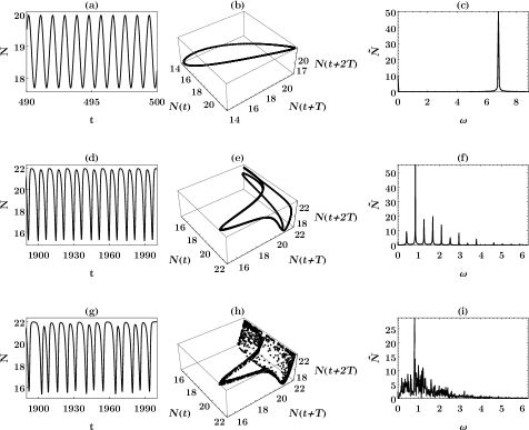
Figure 1: (a,d,g) Total norm (6) as a function of time is shown in the left column, panels (a,d,g). The middle column, panels (b,e,h) show the trajectories in the time-delay diagram (sometimes called phase-portrait), using total norm as a variable. The right column (c,f,i) presents $\tilde{N}(\omega)$ modulus of Fourier transform of the total norm (6). The results correspond to the limit cycle solution with one frequency (with $c=1.74$ - upper row), many frequencies ($c\approx 1.8$ - middle row) and for the chaotic behavior ($c=1.81$ - bottom row).

Several observables may be defined to characterize our system, some of them quite complex. We shall look at first at one of the simplest. This quantity, which is used by us to characterize different kinds of possible states is a total norm defined as

$$N\left(t\right)=\int_{0}^{2\pi}\left[|\Psi_{1}\left(x,t\right)|^{2}+|\Psi_{2}\left(x,t\right)|^{2}\right]\,dx.$$ (6)

Such a norm is preserved in Hermitian systems. Our system is non-conservative and in general the total norm as well as the total energy, and even the topological charge are not necessarily conserved.

Fig. 1 represents graphically typical situations found for a long time dynamics of the system. In the regular regime, say, at $c=1.72$ to $c=1.73$, we observe a stationary behavior with the norm constant in time. In this case it is an antisymmetric state. Upon increasing the coupling $c$ we enter the regime of non-stationary states. For a relatively low coupling we first observe simple regular oscillations (cf. Fig 1a). To extract more information about the system in the non-stationary regime we generate, for particular (characteristic) points on the contour profile plot, a set of figures, including, besides the time evolution of the total norm, also a spatial Fourier transform at the output of the time evolution, supplemented with a time delayed phase portrait. The latter is based on Takens-Mane (TM) theorem takens ; mane which allows us for a projection of the one-dimensional variable onto a multidimensional space (in our case 3D). The dynamics of a chaotic system takes place in some real space which is unavailable to our investigation. The total norm which is here the single observable reflects the one-dimensional projection of the true multi-dimensional evolution. To avoid any artificial crossings of the orbit (caused by the projection – not present in the real dynamics) the so called unfolding is applied according to the TM theorem. More independent variables than one are obtained by using a single scalar variable (in our case the total norm, defined at (6)) calculated at three different instants of time: $t$, $t+T$ and $t+2T$, where $T$ is a predefined delay of time. The excellent discussion of correlations among data points, proper choice of time delay, appropriate number of coordinates and the relation to the average mutual information can be found in abarbanel .

The phase portraits obtained in this way are presented in the middle column in Fig. 1. Note that such an unfolding of a single quantity helps in recognizing the chaotic signatures of motion which are difficult to identify otherwise in the time dynamics. Periodic oscillations of the total norm from Fig. 1a are represented by the solid close circuit trajectory in Fig. 1b. To describe it quantitatively, the Fourier transform of the total norm with respect to time is added in the right panel of Fig. 1c. The spectrum contains a single frequency which corresponds to the period of the norm oscillations. This type of motion can be classified as a non-stationary regular motion with a single period. Upon increasing the coupling $c$, the dynamics of the system becomes more complicated. Oscillations remain regular but are no longer characterized by a single period. Properties of that case are visible in the middle row of Fig.1 (cf. Fig. 1d) for the time evolution of the norm and the system trajectory in Fig. 1e). That behavior is similar to the case presented in the top row but exhibits several oscillations with different periods and is quite typical for the transition towards a fully chaotic motion. Both cases presented in the top and the middle row belong to the class of limit cycles and the system goes from the single frequency behavior (top) to the multi-frequency case (according to the Fig.1f) by the period doubling scenario.

Finally, there exist the limiting value of the coupling parameter where a transition into chaos appears. This is a point where a regular periodic motion transforms into an irregular one, as presented in Fig. 1g. Then the solution in the phase portrait (compare Fig. 1h)) starts to fill a bounded region of the phase space. The multi-frequency solution transforms into the one with a continuous Fourier spectrum as shown in Fig. 1i. The bounded region of dynamics in the phase space results from the volume contraction (typical in dissipative systems) and drives the system to a null-volume chaotic attractor. This is apparent in Fig.1h where phase points are irregularly distributed but the region of their existence is contained in the 2-dimensional manifold. The chaotic system is very sensitive to initial conditions as expected. Even a small perturbation will provide a completely different trajectory.

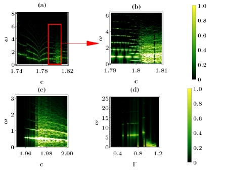
Figure 2: Route to chaos Bifurcation diagram. In panel (a): modulus of the Fourier transform of the total norm, $N(t)$, (see Eq.(6)) for the solution of Eqs.(1), for $\Gamma=1$, $\gamma=1.75$ and $c$ in the range of $\left[1.74,1.82\right]$. In panel (b): magnification of the region enclosed by the red rectangle. Notice the leading frequency component at $\omega\approx 1$ and a narrow stripe around $c\approx 1.808$, where the motion becomes suddenly regular. Panel (c) displays a bifurcation diagram for another route (corresponding to $\Gamma=1$ and $\gamma=2$) versus the control parameter $c$, in the range $\left[1.95,2.0\right]$. In panel (d) the diagram is plotted for fixed $\gamma=2$ and $c=1.98$ for varying $\Gamma\in\left[0.25,1.225\right]$.

The general conclusion that we derive from our necessarily limited studies is that the change of the long time (asymptotic) behavior is rather dramatic and sensitive to the values of parameters. A small change of the chosen control parameter ($c$, $\gamma$ or $\Gamma$) leads to the transition from a regular asymptotic state to a chaotic motion, via a process resembling a standard period doubling scenario, known from classical dynamics of simple low dimensional systems schuster ; strogatz .

We demonstrate such a dramatic transition in Fig. 2a revealing an interesting structure of frequencies in the limit cycle (LC) regime. We highlight the dominant peaks in the Fourier transform of the norm, Eq. (6), as the function of the coupling $c$. The analysis has been done for the range of coupling parameter $c\in\left(1.73,1.83\right]$ (here $\Gamma=1$ and $\gamma=1.75$). For the value of $c$ below the lower bound the system admits regular solutions only. They can be antisymmetric or asymmetric with a constant homogeneous amplitude or even can be inhomogeneous with respect to the spatial coordinate $x$ thus revealing a translational symmetry breaking SciRep . All these solutions are treated within this paper as regular fixed points which are sinks (attractors). We observe regular stationary solutions that are constant in time and the Fourier transform (FT) contains only one central peak with zero frequency. Then the first symmetry breaking occurs and the FT shows single peaks corresponding to the limit cycle state with a single period. For a still bigger $c$ more frequencies appear, still, however, in the limit cycle regime. For $c\approx 1.76$ there is the Hopf bifurcation where a new stable set of frequencies appears at the expense of the former one, which is no longer stable. For bigger values of the control parameter, closer to the chaotic regime, we observe a typical period doubling scenario. At the bifurcation point each branch of the diagram becomes unstable yielding two or more new branches emerging from it. That is the sub-critical bifurcation (phase transition of the first kind), i.e. there is a hysteresis, but states from the backward going branches cannot be observed being unstable. For the $c$ value just above 1.8 we observe a typical chaotic behavior. The spectrum of the frequencies is now smeared over a wide region, ranging from zero up to about 4 (see also Fig. 4a). Additionally one can distinguish bright bands corresponding to leading frequencies. Hence there is still some regularity in the chaotic region. We observe here a certain similarity with the so called exploding solitons introduced by Akhmediev Akhmediev1 ; Akhmediev2 ; Akhmediev3 .

Another interesting feature present in the chaotic regime is a very thin stripe with no chaos. Moreover, for $c$ values bigger than those presented in Figs.2a (and enlarged in Fig. 2b) chaos suddenly disappears. Such a behavior is referred to as a ”crisis” and is a rather common property of chaotic systems. The points of transition from chaos to stable frequencies are typical saddle-node bifurcations, where single stable branches emerge simultaneously with the unstable ones (cf. chaotic scenarios in schuster ).

As a second case we have chosen a path in the different part of the parameter space, with fixed gain and loss amplitudes ($\Gamma=1$ and $\gamma=2$) and the coupling $c$ within the range from $c=1.95$ to $c=2$. The result is shown in Figure 2c again as a plot of FT of the total norm, (6), for asymptotic solutions corresponding to different fixed vales of $c$. Here we observe how the system is approaching chaotic regime, evolving from regular solutions for lower values of $c$ and characterized by a constant norm, entering chaotic region via one subcritical bifurcation. On the other side of the chaotic regime, we observe again an inverse saddle-node bifurcation, exactly as in the previous case.

For a sake of comparison we have investigated another possibilities too, when the coupling value $c$ is fixed and the route to chaos depends either on the gain $\gamma$ or on the loss $\Gamma$ as a variable. The latter scenario is plotted in Fig. 2d and confirms former conclusions formulated for the changing $c$ case. A scenario with changing $\gamma$ is not plotted here but is included in the general map of solutions ($c$ vs $\gamma)$ in the next section.

Transition to chaos may be observed in other dynamical parameters. To exemplify this idea we will refer to the currents mentioned briefly above and introduced in our previous study SciRep . We define current densities along each ring

$$j_{\alpha}(x,t)=\frac{1}{2i}\left(\Psi_{\alpha}^{*}\frac{\partial\Psi_{\alpha}}{\partial x}-\Psi_{\alpha}\frac{\partial\Psi_{\alpha}^{*}}{\partial x}\right),\quad\alpha=1,2$$ (7)

and the current density between the two rings

$$j_{\bot}(x,t)=\frac{c}{2i}\left(\Psi_{1}^{*}\Psi_{2}-\Psi_{1}\Psi_{2}^{*}\right).$$ (8)

For each of these current densities one can define total current by integrating density over the length of the ring. Total currents are obviously functions of time and can be analyzed in the identical manner as we did with the total norm. In particular one can plot Fourier transform of currents for different values of the coupling coefficient. Fig. 3 shows that bifurcation diagrams can be obtained for different dynamical characteristics, if they are non-trivial. For instance in the case illustrated in Fig. 3(a) the current between rings in vanishing and we observe two identical and counter-propagating currents in each ring. When transformed to the Fourier space they may be used as chaos indicator instead of the total norm. In the case shown in Fig. 3(b) and Fig. 3(c) both currents exist and they contain the same information as far as the onset of chaos is concerned.

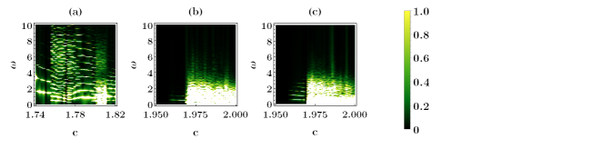
Figure 3: Bifurcation diagram of the route to chaos obtained from the total current. In panel (a) we plot Fourier transform of the current in each ring corresponding to Fig. 2(a), for $\Gamma=1$ and $\gamma=1.75$. Panels (b) and (c) correspond to Fig. 2(c) with $\Gamma=1$ and $\gamma=2$ and present Fourier transforms of the total current in one of the rings and between rings, respectively.

4 Galerkin approximation. Few modes model.

The number of explicitly given analytical solutions of (1) covers only a small fraction of available possibilities. To capture the essence of the transition from a regular behavior to the chaotic regime we apply the so called Galerkin approximation (GA) SciRep ; Ern ; galerkin ; Chekroun ; Wanga ; GA-Malomed ; Driben16 ; Wang17 . The idea of GA is based on the observation that due to the periodic boundary conditions only certain $k$ vectors participate in the dynamics. It turns out that full continuous dynamics can be well approximated and viewed as the interaction of (small) number of modes, even in the chaotic regime. The computational problem is then reduced to a solution of few ordinary differential equations instead of considering the full model described numerically by partial differential equations. That allows us to save the computational time and the results can be obtained very efficiently. The wavefunction in each ring may be expressed in terms of Fourier series

$$\psi_{\alpha}\left(x,t\right)=\sum_{n=-\infty}^{\infty}B_{\alpha,n}\left(t\right)e^{\mathrm{i}nx},$$ (9)

where $\alpha={1,2}$ denotes the rings. While in SciRep these solutions were expressed in the stationary form with all amplitudes $B_{\alpha,n}$ independent of time, in general, they can be time dependent. By substituting (9) into (1) one obtains

$$\mathrm{i}\frac{\mathrm{d}B_{1,n}}{dt}=\left(\mathrm{i}\gamma+n^{2}\right)B_{1,n}+\left(1-\mathrm{i}\Gamma\right)\sum_{k=-l}^{l}\sum_{m=-l}^{l}B_{1,k+m-n}^{\ast}B_{1,k}B_{1,m}+cB_{2,n}$$

$$\mathrm{i}\frac{\mathrm{d}B_{2,n}}{dt}=\left(\mathrm{i}\gamma+n^{2}\right)B_{2,n}+\left(1-\mathrm{i}\Gamma\right)\sum_{k=-l}^{l}\sum_{m=-l}^{l}B_{2,k+m-n}^{\ast}B_{2,k}B_{2,m}+cB_{1,n}$$ (10)

where $2l+1$ is the number of modes taken into account. It turns out that restricting the dynamics to just a few modes (typically we take $l=5$) is sufficient. The GA gives an excellent agreement with the full system predictions. In particular the Fourier spectra in the case of a limit cycle behavior, both for the single frequency and the multi-frequency cases [shown, respectively, in Fig. 1c and Fig. 1f], calculated solving GPE (1) and using GA are practically indistinguishable. It is directly illustrated in Fig. 4a and Fig. 4b, where a side-by side comparison of dynamics in the time domain is plotted. In addition Fourier spectra of both full dynamics ($\tilde{N}_{1}$) and GA ($\tilde{N}_{2}$) may be determined, again demonstrating close similarity as shown in Fig. 4c and in the lower row of panels, where we present the relative error defined as $\Delta\tilde{N}/\tilde{N}_{tot}=(\tilde{N}_{1}-\tilde{N}_{2})/(\tilde{N}_{1}+\tilde{N}_{2})$. More importantly, the bifurcation diagrams (as those presented in Fig. 2) obtained using GPE solutions and the GA agree fully within our resolution accuracy.

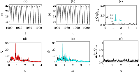
Figure 4: Side-by-side comparison of a time evolution in the quasi-periodic case ($c=1.799$) obtained by means of (a) numerics, (b) with the Galerkin approximation. (c) The relative error between Fourier spectra in the time domain for the total norm presented in (a) and (b) with inset presenting directly the agreement between both functions. Bottom row: the behavior of the system in the chaotic regime at $c=1.81$. Panel (d) shows a comparison of Fourier spectra for numerical simulations with two different initial perturbations; panel (e) an analogical comparison between two spectra taken from numerical simulations (black), and GA (cyan). Panel (f) – the same as in (c) for the chaotic behavior case.

The difference between GA and GPE numerics becomes non negligible when the comparison is done in the chaotic regime (compare Fig.4e). Both spectra present qualitatively the same behavior, but cannot be identical, due to the critical sensitivity to the initial conditions in the chaotic regime. Notice that the main peaks obtained using both methods are similar and the differences appear in the magnitudes of less important peaks. Interestingly, the same degree of ”disagreement” is present when two numerical simulations, obtained for slightly different initial perturbations, or more generally for slightly different initial conditions (cf. Fig.4d) are compared. In order to better illustrate discrepancies between both spectra in Fig. 4f the relative error is presented in analogy to Fig. 4c. The finite numerical accuracy of GPE solution as well as a truncation of the expansion (9) leads to a noisy behavior. It can be compared with the quasi-periodic case with spectrum in Fig. 1f. As shown in Fig. 4d for quasi-periodic case, the relative error is zero almost in the whole range of the spectrum. That confirms the very good agreement between GA and numerics in this case (the GA spectrum is shown in the inset).

From the above studies we conclude that GA shows practically the same dynamics as our original system, and all final, asymptotic states are identical in both cases. Thus the dynamics of two one dimensional coupled rings may be reduced to a system of coupled oscillators. This reduction allows to apply GA to obtain two-dimensional map of final states with varying $c$ and $\gamma$ (the case with varying $\Gamma$ has been studied numerically and presented in Fig. 2d). From the physical point of view, the relation between gain and loss ($\gamma/\Gamma$) is significant. Hence, without a loss of generality, we present an analysis of solutions in 2D plane $c-\gamma$ for fixed $\Gamma=1$ in Fig. 5 (left-top panel). As an input we apply (5) with the excitation of all perturbation modes in a range $l\in\left[-5,5\right]$. It is hence a symmetric state with an antisymmetric perturbation. In the bottom row of Fig. 5 cross-sections of that map for two particular values $\gamma=2$ and $\gamma=1.75$ are compared. In the top row the initial perturbation contains excitations of all modes between -5 and 5, while in the middle row the perturbation is magnified 5 times. The bottom row corresponds to the same perturbation amplitude like in the top row, however, only odd modes in the range $\left[-5,5\right]$ are excited.

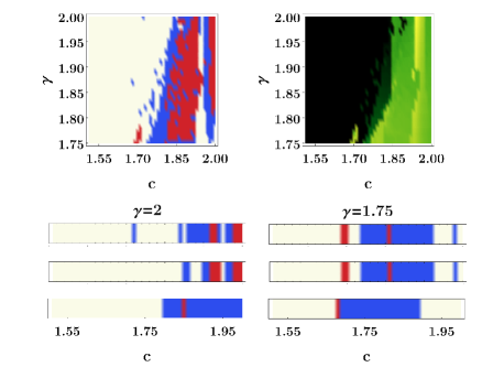
Figure 5: Top-left panel: A map of final states for a symmetric input with antisymmetric perturbation (excitation of all perturbation modes between $l=-5$ and $l=5$), Blue (red) color denotes limit-cycle states (chaotic solutions). In the white area stationary regular solutions exist only. Top-right panel: the maximal positive Lyapunov displayed for solutions in the top-left map. Bottom: cross-sections of the top-left map for $\gamma=2$ (left) and $\gamma=1.75$ (right); each row corresponds to the different initial perturbation: the top row: all $l=-5$ to $l=5$ modes are perturbed, the middle row: the same for 5 times stronger perturbation, the bottom row: only odd modes in $[-5,5]$ interval were perturbed.

Furthermore, to quantify the chaotic behavior, the maximal positive Lyapunov exponents have been determined in the same map ($c-\gamma$). The calculation utilizes (10) where each amplitude is assumed to take the form

$$B_{\alpha,n}\left(t\right)=e^{-i\mu t}\left[B_{\alpha s,n}\left(t\right)+e^{\lambda t}U_{\alpha,n}+e^{\lambda^{\ast}t}V_{\alpha,n}^{\ast}\right],$$ (11)

where index $\alpha=\left\{1,2\right\}$ pertains to the ring number, $n$ is an order of the amplitude in the Fourier expansion (9) and the subscript $s$ denotes the exact solution of the system (10). Amplitudes of the perturbation should be small, i.e. $U_{\alpha,n},V_{\alpha,n}\ll B_{\alpha s,n}$. For simplicity of calculations we assume that the perturbation depends on time only via an exponential expression with $\lambda$ being Lyapunov exponent. Any out-of-equilibrium state (including chaotic one) is detected by a real, positive value of $\lambda$ and is plotted in the top-right panel of Fig. 5. Generally, the existence of the area of positive exponents and its location confirms former results and is in a relatively good agreement with non-stationary states plotted in the left panel of Fig.5.

5 Conclusions

The model of two coupled nonlinear Schrödinger equations with a linear gain and a nonlinear loss has been investigated. Such a system may physically correspond to models of microresonator nanostructures, polariton condensates or coupled optical waveguides. Our model may also represent systems with saturation and linear loss. It seems suitable for description of quantum circulation in a macroscopic polariton spinor ring condensate Snoke . And last but not least, it can be extended to study the dynamics of more complicated structures involving inhomogeneous coupling and stripe of coupled rings or matrix of rings.

We have studied in detail a family of non-stationary oscillating states and a transition from regular solutions to chaotic ones caused by changing one control parameter. On the route to chaos regular non-stationary states (limit cycles) can be observed, characterized by a single or multi-frequencies. As we sweep the value of the coupling from small to large values we encounter many bifurcation types like saddle-node bifurcation (also in the inverse realization), as well as period doubling and Hopf bifurcation. All our numerical results from the ”full” model (using equations (1)) are quantitatively indistinguishable from that obtained using a few-modes model - obtained by introducing the Galerkin Approximation. It allows to limit the number of degrees of freedom of the system to the most relevant ones and transforms the problem into a set of nonlinearly coupled modes. This reduction let us investigate characteristics of the system more effectively and is the manifestation of the correspondence between the continuous operator problem and its discrete representation.

We have visualized different routes to chaos in our non-hermitian system using simple global variables such as the norm of the studied field $\Psi$ analyzing both the Fourier transform of the norm as well as its time delay diagram. Interestingly the transition to chaos may be also observed in the dynamics of the probability currents flowing between the studied rings.

References

- [1] Smith, R. G., Optical power handling capacity of low loss optical fibers as determined by stimulated Raman and Brillouin scattering, Appl. 11, 2489, (1972).
- [2] Agrawal, G. P., Nonlinear Fiber Optics, 3rd edition, Academic Press, SanDiego, CA, (2001).
- [3] Boyd, R. W., Nonlinear Optics, Academic Press, SanDiego, CA, (1992).
- [4] L. Deng, E.W. Hagley, J. Wen, M. Trippenbach, Y. Band, P.S. Julienne, Four-wave mixing with matter waves, Nature 398, 218 (1999).
- [5] M. Trippenbach, Y. Y. Band, M. Edwards, M. Doery, P S Julienne, E W Hagley, L Deng, M Kozuma, K Helmerson, S L Rolston and W D Phillips, Coherence properties of an atom laser, J. Phys. B 33, 47 (2000).
- [6] Konstantinos Lagoudakis, The Physics of Exciton-Polariton Condensates, EPFL Press,CRC Press, (2013).
- [7] Fabrice P. Laussy, Vladislav Timofeev, Daniele Sanvitto, Exciton Polaritons in Microcavities: New Frontiers, Springer-Verlag Berlin Heidelberg (2012).
- [8] H. Deng, G. Weihs, C. Santori, J. Bloch, and Y. Yamamoto, Condensation of Semiconductor Microcavity Exciton Polaritons, Science 298, 199 (2002).
- [9] J. Kasprzak, M. Richard, S. Kundermann, A. Baas, P. Jeambrun, J. M. J. Keeling, F. M. Marchetti, M. H. Szymanska, R. Andre, J. L. Staehli, V. Savona, P. B. Littlewood, B. Deveaud and Le Si Dang, Bose-Einstein condensation of exciton polaritons, Nature 443, 409 (2006).
- [10] R. B. Balili, V. Hartwell, D. Snoke, L. Pfeiffe, and K. West, Bose-Einstein Condensation of Microcavity Polaritons in a Trap, Science 316, 1007 (2007).
- [11] H. Deng, H. Haug, Y, Yamamoto, Exciton-polariton Bose-Einstein condensation, Rev. Mod. Phys., 82, 1489 (2010).
- [12] T. Byrnes, Na Young Kim, Y. Yamamoto, Exciton-polariton condensates, Nature Physics 10, 10:13 (2014).
- [13] Sun Y, Fan X, Optical ring resonators for biochemical and chemical sensing, Anal Bioanal Chem. 399, 205 (2011).
- [14] V. B. Braginsky, M. L. Gorodetsky, and V. S. Ilchenko, Quality-factor and nonlinear properties of optical whispering-gallery modes, Phys. Rev. A 137, 393 (1989).
- [15] F. C. Blom, D. R. van Dijk, H. J. Hoekstra, A. Driessen, and Th. J. A. Popma, Experimental study of integrated-optics microcavity resonators: toward an all-optical switching device, Appl. Phys. Lett. 71, 747 (1997).
- [16] E. J. Post, Sagnac Effect, Rev. Mod. Phys. 39, 475 (1967).
- [17] J. C. Knight, H. S. T. Driver, R. J. Hutcheon, and G. N. Robertson, Core-resonance capillary-fiber whispering-gallery-mode laser, Opt. Lett. 17, 1280 (1992).
- [18] Y. Yamamoto and v Slusher, Optical Processes in microcavities, Phys. Today 46, 66 (1993).
- [19] T. Herr, V. Brasch, J. D. Jost, C. Y. Wang, N. M. Kondratiev, M. L. Gorodetsky and T. J. Kippenberg, Temporal solitons in optical microresonators, Nature Photonics 8, 145 (2014).
- [20] H. Guo1, M. Karpov, E. Lucas, A. Kordts, M. H. P. Pfeiffer, V. Brasch, G. Lihachev, V. E. Lobanov, M. L. Gorodetsky and T. J. Kippenberg, Universal dynamics and deterministic switching of dissipative Kerr solitons in optical microresonators, Nat. Phys. 13, 94 (2017).
- [21] E. Lucas, M. Karpov, H. Guo, M.L. Gorodetsky and T.J. Kippenberg, Breathing dissipative solitons in optical microresonators, Nat. Commun, 8 736 (2017).
- [22] Yu, M. et al. Breather soliton dynamics in microresonators Nat. Commun. 8, 14569 (2017).
- [23] Kerry Vahala, Optical microcavities, World Scientific Publishing, Singapore (2004).
- [24] Steven T. Cundiff, New generation of combs, Nature 450, 1175 (2007).
- [25] T. J. Kippenberg, R. Holzwarth, S. A. Diddams, Microresonator-based optical frequency combs, Science 332, 555-559 (2011).
- [26] M. L. Gorodetsky, V. E. Lobanov, G. Lihachev, N. Pavlov, S. N. Koptyaev, Kerr combs in microresonators: from chaos to solitons and from theory to experiment, Proceedings of the SPIE, Vol. 10090, pp.100900H-1 (2017).
- [27] N.V. Hung, K.B. Zegadlo, A. Ramaniuk, V.V. Konotop, and M. Trippenbach, Modulational instability of coupled ring waveguides with linear gain and nonlinear loss, Sci. Rep. 7 4089, (2017).
- [28] Aleksandr Ramaniuk, Nguyen Viet Hung, Michael Giersig, Krzysztof Kempa, Vladimir V. Konotop and Marek Trippenbach,Vortex Creation without Stirring in Coupled Ring Resonators with Gain and Loss, Symmetry 10 195, (2018).
- [29] Alexandre Ern and Jean-Luc Guermond, Theory and practice of finite elements, Springer 2004.
- [30] B.G. Galerkin, On electrical circuits for the approximate solution of the Laplace equation Vestnik Inzh. 19 897, (1915).
- [31] M. D. Chekroun, M. Ghil, Honghu Liu, and Shouhong Wang, Low-Dimensional Galerkin Approximations of Nonlinear Delay Differential Equations, Discrete and Continuous Dynamical Systems 36, 4133-4177 (2016).
- [32] Y.-S. Wanga, C.-S. Chien, A spectral-Galerkin continuation method using Chebyshev polynomials for the numerical solutions of the Gross - Pitaevskii equation, Journal of Computational and Applied Mathematics 235, 2740-2757 (2011).
- [33] T. Bland, N.G. Parker, N.P. Proukakis, and B.A. Malomed, Probing quasi-integrability of the Gross - Pitaevskii equation in a harmonic-oscillator potential, J. Phys. B: At. Mol. Opt. Phys. 51 205303, (2018).
- [34] R. Driben, V. V. Konotop, B. A. Malomed, and T. Meier, Dynamics of dipoles and vortices in nonlinearly coupled three-dimensional field oscillators, Phys. Rev. E 94 012207, (2016).
- [35] J. Wang, Y. Zhou, and X. Liu, A space-time fully decoupled wavelet Galerkin Method for solving multidimensional nonlinear Schrodinger equations with damping, Math. Problems in Eng. 11 1, (2017).
- [36] Igor Kukavica, Kerem Ugurlu, and Mohammed Ziane, On the Galerkin approximation and strong norm bounds for the stochastic Navier-Stokes equations with multiplicative noise, Differential Integral Equations 31, 173 (2018)
- [37] E. Thiede, D. Giannakis, A. R. Dinner, J. Weare, Galerkin approximation of dynamical quantities using trajectory data, arXiv:1810.01841
- [38] A. Kosiorek, W. Kandulski, P. Chudzinski, K. Kempa, and M. Giersig, Shadow Nanosphere Lithography: Simulation and Experiment, Nano. Let. 4, 1359 (2004).
- [39] A. Sigler and B. A. Malomed, Solitary pulses in linearly coupled cubic-quintic Ginzburg-Landau equations, Physica D 212, 305 (2005).
- [40] F. Takens (1981). Detecting strange attractors in turbulence. In D. A. Rand and L.-S. Young. Dynamical Systems and Turbulence, Lecture Notes in Mathematics, vol. 898. Springer-Verlag. pp. 366-381.
- [41] R. Mane (1981). On the dimension of the compact invariant sets of certain nonlinear maps. In D. A. Rand and L.-S. Young. Dynamical Systems and Turbulence, Lecture Notes in Mathematics, vol. 898. Springer-Verlag. pp. 230-242.
- [42] Abarbanel, H.D.I., Analysis of observed chaotic data, Springer 1995.
- [43] N. Akhmediev, J. M. Soto-Crespo, and G. Town, Pulsating solitons, chaotic solitons, period doubling, and pulse coexistence in mode-locked lasers: Complex Ginzburg-Landau equation approach, Phys. Rev E,63, 056602 (2001).
- [44] Akhmediev, N., Ankiewicz, A.(Eds.), Dissipative Solitons: From Optics to Biology and Medicine, Lect. Notes Phys. 751 (Springer, Berlin Heidelberg 2008).
- [45] Philippe Grelu (Eds.) Nonlinear Optical Cavity Dynamics: From Microresonators to Fiber Lasers, Wiley (2016).
- [46] H.-G. Schuster and W. Just, Deterministic Chaos: An Introduction, Wiley-VCH 1995.
- [47] Strogatz, S.H., Nonlinear dynamics and chaos: With applications to physics, biology, chemistry and engineering, Perseus Book Publishing 1994.
- [48] Gangqiang Liu, David W. Snoke, Andrew Daley, Loren N. Pfeiffer, and Ken West, A new type of half-quantum circulation in a macroscopic polariton spinor ring condensate, PNAS 112, 2676 (2015).