Constraining the Neutron Star Radius with Joint Gravitational-Wave and Short Gamma-Ray Burst Observations of Neutron Star–Black Hole Coalescing Binaries

Abstract

Coalescing neutron star (NS)- black hole (BH) binaries are promising sources of gravitational-waves that are predicted to be detected within the next few years by current GW observatories. If the NS is tidally disrupted outside the BH innermost stable circular orbit, an accretion torus may form, and this could eventually power a short gamma-ray burst (SGRB). The observation of an SGRB in coincidence with gravitational radiation from an NS-BH coalescence would confirm the association between the two phenomena and also give us new insights into NS physics. We present here a new method to measure NS radii and thus constrain the NS equation of state using joint SGRB and GW observations of NS-BH mergers. We show that in the event of a joint detection with a realistic GW signal-to-noise ratio (S/N) of $10$, the NS radius can be constrained to $\lesssim 20$% accuracy at 90% confidence.

1 Introduction

The first observation of a binary BH merger in GWs made by Advanced LIGO, GW150914, marked the dawn of the GW astronomy era (Abbott et al., 2016b). Subsequently, the LIGO-Virgo Collaboration reported other nine binary BH merger observations (Abbott et al., 2016a, 2017c, 2017d, 2017e, 2018), and the detection of GW170817, a signal that is consistent with a binary NS inspiral (Abbott et al., 2017f). Hinderer et al. (2018) showed that NS-BH systems with certain parameter combinations are also consistent with the GW and electromagnetic (EM) observations of GW170817.

Second-generation GW detectors — i.e., Advanced LIGO (Aasi et al., 2015a), Virgo (Acernese et al., 2015), KAGRA (Aso et al., 2013), and LIGO-India (Iyer et al., 2011; Unnikrishnan, 2013) — will also be able to detect the GW radiation emitted by NS-BH coalescing binaries, a category of compact binary that remains to be observed. In addition to GWs, among the reasons of interest in coalescing NS-BH binaries is the possibility that if the NS is tidally disrupted outside the innermost stable circular orbit (ISCO) of its BH companion, matter can be accreted onto the BH, powering a SGRB (Nakar, 2007). We now know that a binary NS merger can power an SGRB (Abbott et al., 2017b), and future joint GW-EM observations will be able to determine whether this is true for NS-BH systems too. Naturally, such observations are intrinsically challenging due to the low expected GW-SGRB joint detection rate for NS-BH binaries. This is predicted by Clark et al. (2015) to be $0.4$–$10\,\mathrm{yr^{-1}}$ for LIGO-Virgo at design sensitivity and an idealized SGRB observing facility with all-sky coverage, in line with earlier results from Nissanke et al. (2013) (up to $3\,\mathrm{yr^{-1}}$ with a three detector network when ignoring source inclination requirements). The estimate drops to $0.03$–$0.7\,\mathrm{yr^{-1}}$ when considering the Swift field of view. For comparison, Wanderman & Piran (2015) calculated joint detection rates with Swift and Fermi of $0.3$–$1.4\,\mathrm{yr^{-1}}$ and $3$–$10\,\mathrm{yr^{-1}}$, respectively, while Regimbau et al. (2015) determined $0.001$–$0.16\,\mathrm{yr^{-1}}$ in the case of Swift. The assumptions behind these frameworks are different and we refer the interested reader to the original articles for details. The upcoming third generation of GW detectors, however, will have a much larger observational horizon (up to $z\simeq 4$ for NS-BH binaries) which automatically increases the joint detection rate considerably (Punturo et al., 2010; Abernathy et al., 2011; Kalogera et al., 2019; Sathyaprakash et al., 2019). Further interest in NS-BH binaries is due to the possibility that the tidally disrupted material is ejected away from the NS-BH system, generating an EM transient powered by the decay of $r$-process ions (macronova) (Li & Paczyński, 1998; Kulkarni, 2005; Metzger et al., 2010; Metzger & Berger, 2012; Fernández & Metzger, 2016; Metzger, 2017). Similar to the SGRB case, recent GW-EM observations of GW170817 have confirmed that binary NSs are sites that host $r$-processes (Abbott et al., 2017g, a), but whether this holds for NS-BH binaries as well, remains to be proven observationally.

Whether the NS in an NS-BH binary undergoes tidal disruption or not, and the amount of matter that is available for accretion (or to feed into the ejecta) in the event of a tidal disruption, both depend on the physical properties of the BH (mass and spin) and of the NS, including the currently unknown equation of state (EOS) that regulates the microphysics of the NS (Pannarale et al., 2011; Foucart, 2012; Foucart et al., 2018). The GW radiation of coalescing NS-BH systems also depends on the source properties, and among them is the NS EOS (Bildsten & Cutler, 1992; Kokkotas & Schafer, 1995; Vallisneri, 2000; Shibata et al., 2009; Duez et al., 2010; Kyutoku et al., 2010, 2011; Lackey et al., 2012, 2014; Foucart et al., 2013, 2014; Pannarale et al., 2013, 2015b, 2015a; Kawaguchi et al., 2015; Hinderer et al., 2016; Kumar et al., 2017; Dietrich et al., 2018), but it may be hard to constrain the NS EOS with NS-BH GW inspiral signals only (Pannarale et al., 2011). Therefore, the GW and EM emission of NS-BH binaries that undergo tidal disruption will carry information about all the properties of the progenitor system, and hence about the NS EOS.

Pannarale & Ohme (2014) showed how joint GW and SGRB observations of NS-BH coalescences may provide invaluable information about the NS EOS. On the basis of this observation, we propose a method to exploit such observations in order to constrain the NS radius, and thus the NS EOS. In the scenario in which NS-BH systems are progenitors of SGRB central engines, it is reasonable to expect the SGRB energy to be proportional to the rest mass of the torus that accretes onto the remnant BH. In turn, this mass can be expressed as a function of the mass and spin of the BH initially present in the binary, and the NS mass and radius (Foucart, 2012; Foucart et al., 2018). Our method explores the portion of parameter space that is pinpointed by the GW observation — GW Bayesian inference provides posterior distributions for the two masses and the BH spin — and thus determines a posterior distribution for the NS radius by imposing the condition that the merger yields a torus sufficiently massive to power the observed SGRB energy.

Assuming an SGRB isotropic energy of $E_{\gamma,{\rm ISO}}=10^{51}\,$erg, we expect to be able to measure the NS radius (at 90% confidence) with $\lesssim 20$% accuracy, given a GW detection with a S/N of $10$. This measure is expected to improve for less energetic SGRBs and GWs with higher S/N. We show that the poorly known parameters that our analysis marginalizes over — such as the mass-energy conversion efficiency for the SGRB — have a negligible impact on our results, provided the SGRB energy is sufficiently low. Our method is well behaved even for (non-isotropic) energies as high as $E_{\gamma}=10^{50}\,$erg, thus the restriction is not very limiting.

The paper is organized as follows. In Sec. 2 we describe our method in detail, discussing the poorly constrained parameters involved in the analysis. In Sec. 3 we test the method and present the results we obtained by simulating joint GW-SGRB observations. Finally, in Sec. 4 we draw our conclusions.

Throughout the paper, we assume geometric units ($G=c=1$), unless otherwise explicitly noted.

2 Methodology

When an NS undergoes tidal disruption during an NS-BH coalescence, part of the matter that constitutes it may remain outside the BH up to a few milliseconds after the merger. We denote the mass of this remnant matter by $M_{\rm rem}$. A small fraction of this will form unbound ejecta that can eventually power EM transients by radioactive decay of $r$-process heavy ions (Li & Paczyński, 1998; Kulkarni, 2005; Metzger et al., 2010; Metzger & Berger, 2012; Fernández & Metzger, 2016; Metzger, 2017). The rest of it will stay bound around the BH, forming a neutrino-cooled accretion disk and a tidal tail, orbiting with high eccentricity, which will fall back, filling the disk on a timescale of $0.1$–$1$ s (Foucart, 2012). The remnant BH and the disk form a system that is a plausible candidate for the central engine of (a fraction of) SGRBs, as the accretion of mass from the disk onto the BH could power the launch of a relativistic jet (Eichler et al., 1989; Paczynski, 1991; Meszaros & Rees, 1992; Narayan et al., 1992; Mészáros, 2006; Lee & Ramirez-Ruiz, 2007).

Given a disk of mass $M_{\rm disk}$, the energy radiated in gamma rays during the prompt emission by conversion of mass corresponds to

$$E_{\gamma}=\epsilon M_{\rm disk}\,,$$ (1)

where $\epsilon$ is the mass-energy conversion efficiency. $E_{\gamma}$ is related to the SGRB isotropic energy $E_{\gamma,{\rm ISO}}$ by

$$E_{\gamma}=(1-\cos{\theta_{\rm j}})E_{\gamma,{\rm ISO}}$$ (2)

where $\theta_{\rm j}$ is the jet half-opening angle, i.e. its beaming angle. In this work, we assume $E_{\gamma,{\rm ISO}}$ to be measured from the gamma-ray flux, provided the distance to the host galaxy of the SGRB is known. We may therefore write

$$(1-\cos{\theta_{\rm j}})E_{\gamma,{\rm ISO}}=\epsilon M_{\rm disk}\,.$$ (3)

Assuming the gravitational radiation emitted by the coalescence is also observed, one can exploit this last equation to connect the measured $E_{\gamma,{\rm ISO}}$ and the NS-BH properties inferred from the GW measurement (masses and spins of the binary constituents, as discussed later on in this section) in order to constrain the NS radius, and hence the NS EOS.

Two unknowns are evident in Eq. (3). The first one is the efficiency $\epsilon$, which varies from system to system and is determined by a chain of complicated physical processes, the nature of which is an open field of investigation (see, e.g., Nakar (2007) and Lee & Ramirez-Ruiz (2007), and references therein). The treatment of $\epsilon$ in our analysis is discussed in Sec. 3.3.1. The second unknown is the beaming angle $\theta_{\rm j}$. While this can be inferred by measuring the time at which a jet break appears in the afterglow light curve (Sari et al., 1999), usually SGRB jet breaks are not observed and only lower limits ($\theta_{\rm j}\gtrsim 3^{\circ}$) can be placed (Berger, 2014). This happens because (i) SGRB afterglows are fainter than long gamma-ray burst (GRB) afterglows, and because (ii) their light curves typically drop below a detectable level within a day. We therefore treat $\theta_{\rm j}$ as an unknown parameter in our analysis, as detailed further in Sec. 3.3.2.

The last element entering Eq. (3) is the disk mass $M_{\rm disk}$, and we make the approximation $M_{\rm disk}\simeq M_{\rm rem}$ (i.e., we neglect the mass of the possible ejecta). This approximation is justified by the results of numerical-relativity simulations, which predict ejecta masses of at most $\sim\mathcal{O}(10^{-2}\,M_{\odot})$ (Kawaguchi et al., 2015; Kyutoku et al., 2015; Kawaguchi et al., 2016; Foucart et al., 2017) and total remnant masses that are an order of magnitude higher in such extreme cases (Kyutoku et al., 2011; Foucart, 2012; Foucart et al., 2017).

We express $M_{\rm rem}$ using the semi-analytical formula of Foucart et al. (2018), which updates a formula previously introduced in Foucart (2012) and is obtained by fitting results of fully relativistic numerical-relativity simulations. Specifically, the fraction of NS matter that remains outside the remnant BH is given by

$$\frac{M_{\rm rem}}{M_{\rm b,NS}}=\Bigl{[}\alpha\frac{1-2C_{\rm NS}}{\eta^{1/3}}-\beta\hat{R}_{\rm ISCO}\frac{C_{NS}}{\eta}+\gamma\Bigr{]}^{\delta}\,,$$ (4)

where $M_{\rm b,NS}$ is the baryonic mass of the NS, $\eta=M_{\rm BH}M_{\rm NS}/(M_{\rm BH}+M_{\rm NS})^{2}$ is the symmetric mass ratio ($M_{\rm BH}$ and $M_{\rm NS}$ being the gravitational mass of the BH and the NS, respectively), $R_{\rm NS}$ is the radius of the NS at isolation expressed in Schwarzschild coordinates, $C_{\rm NS}=M_{\rm NS}/R_{\rm NS}$ is the NS compactness, $\chi_{\rm BH}$ is the dimensionless spin magnitude of the BH in the NS-BH binary, $\hat{R}_{\rm ISCO}=R_{\rm ISCO}/M_{\rm BH}$ is the normalized ISCO radius, and $\alpha=0.406$, $\beta=0.139$, $\gamma=0.255$, $\delta=1.761$ are the free coefficients determined by the fitting procedure. The ISCO radius $R_{\rm ISCO}$ is a function of the mass $M_{\rm BH}$ and spin magnitude $\chi_{\rm BH}$ of the BH in the original NS-BH binary (Bardeen et al., 1972).

The discussion carried out so far can be summarized as follows: an NS-BH coalescence can result in an SGRB with energy proportional to the rest mass liberated by the tidal disruption and given by Eq. (4). The system of equations laid out is closed by prescribing an EOS for the NS. This enters the expression(s) for the remnant mass through $R_{\rm NS}$ and $M_{\rm b,NS}$. Given that our goal is to determine a method to constrain the NS EOS on the basis of a joint GW-SGRB observation of an NS-BH coalescence, the EOS is ultimately the unknown we would want to solve for, under the constraints imposed by the observational data. In order to simplify this task and to avoid repeatedly solving the Tolman-Openheimer-Volkoff NS structure equations (Oppenheimer & Volkoff, 1939; Tolman, 1939), we express the NS baryonic mass $M_{\rm b,NS}$ as a function of the NS gravitational mass $M_{\rm NS}$ and solve for $R_{\rm NS}$. In this sense, our method constrains the NS radius and indirectly constrains the NS EOS.

The approximation we use to relate $M_{\rm NS}$ to $M_{\rm b,NS}$ is the fit to NS equilibrium sequences provided by Cipolletta et al. (2015):

$$\frac{{M}_{\rm b,NS}}{M_{\odot}}=\frac{{M}_{\rm NS}}{M_{\odot}}+c_{2}\left(\frac{M_{\rm NS}}{M_{\odot}}\right)^{2}\,.$$ (5)

The value of the free coefficient $c_{2}=13/200$ found by Cipolletta and collaborators is biased by their choice of EOSs used to build the NS equilibrium sequences they fit with Eq. (5). We find that, for a large sample of EOSs, acceptable values of $c_{2}$ lie in the range $[12/200,23/200]$ as shown in Fig. 1, where we only show six representative EOSs to avoid overcrowding the figure.

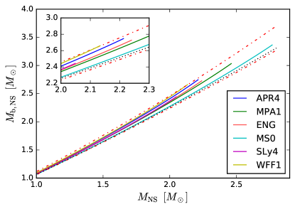
Figure 1: Baryonic-gravitational mass relations along stable NS equilibrium sequences obtained with different EOSs (continuous curves). The black dotted line is the fit in Eq. (5) with its original value $c_{2}=13/200$ Cipolletta et al. (2015). The red dotted-dashed lines correspond instead to $c_{2}=\{12/200,23/200\}$ (lower and upper curve, respectively). These two values allow us to enclose all the NS equilibrium sequences.

Given the observation of an NS-BH coalescence, GW parameter estimation provides posterior probability distributions for the gravitational masses and the BH spin that enter Eq. (4). Once we obtain the raw posterior distribution samples from the GW analysis, we “prune” them as follows. We discard all parameter points that do not satisfy the requirements $M_{1}>3\,M_{\odot}$ (i.e., the primary object is presumably not a BH because it is not massive enough), $M_{2}<2.8\,M_{\odot}$ and $\chi_{2}<0.4$ (i.e., the secondary object is presumably not an NS because its mass and/or spin are too high) . This step allows us to downsample the posteriors of the GW measurement to a set of points reasonably compatible with the assumption that the observed SGRB was due to an NS-BH progenitor.

After the pruning of the GW posteriors, we determine a posterior for the NS radius $R_{\rm NS}$ as follows. We randomly sample the joint GW posterior distribution for $M_{\rm NS}$, $M_{\rm BH}$ and $\chi_{\rm BH}$ (effectively using it as an informed prior in a hierarchical analysis), and assume uniform prior distributions for $R_{\rm NS}$ and the remaining unknowns in our setup, i.e., $\epsilon$, $c_{2}$ and $\cos\theta_{\rm j}$. From Eq. (3) we thus obtain a distribution for $E_{\gamma,{\rm ISO}}$. Each value of this distribution is then compared to $E_{\gamma,{\rm ISO}}^{\rm obs}$, which is the measured value of $E_{\gamma,{\rm ISO}}$. We then reject any sample point that yields an energy that differs by more than a given tolerance $\tau$ from the observed $E_{\gamma,{\rm ISO}}$, according to the condition

$$\frac{|E_{\gamma,{\rm ISO}}-E_{\gamma,{\rm ISO}}^{\rm obs}|}{E_{\gamma,{\rm ISO}}^{\rm obs}}>\tau$$ (6)

Here $\tau$ accounts both for an uncertainty on the observed SGRB energy and for errors introduced by using the approximate formula in Eq. (4), which Foucart et al. (2018) reported to be $\sim 15\%$. We also reject any sample point that yields a violation of the causality condition $R_{\rm NS}\geq 3.04\,GM_{\rm NS}/c^{2}$ (Lattimer et al., 1990; Glendenning, 1992).

It is important to stress that although the GW signal alone can bring information on $R_{\rm NS}$ (e.g., via the tidal deformability of the star), this information is not exploited by our method, in order to keep our analysis as agnostic as possible. While this constitutes a loss of information, we avoid introducing systematic errors due to the modeling of the EOS imprints on the GW signal waveform. We will explore the benefits of using the full GW information in a future study.

The building blocks of our method are summarized as follows:

• Parameter estimation on the GW signal to obtain posterior distribution on the signal parameters. Among these, $M_{1}$ (mass of the primary star), $M_{2}$ (mass of the secondary star), and $\chi_{1}$ (spin of the primary star) are those that will directly enter in our analysis. An example of this is provided in Section 3.2.

• The posterior distribution of GW signal parameters is “pruned” to reject all the parameter combinations incompatible with a NS-BH system. The criterion involves conditions on $M_{1}$ , $M_{2}$, and $\chi_{2}$ (spin of the secondary star) described earlier in this section. After this step we can set $M_{1}=M_{\rm BH}$, $M_{2}=M_{\rm NS}$ and $\chi_{1}=\chi_{\rm BH}$.

• We use the distributions of $M_{\rm NS}$, $M_{\rm BH}$ and $\chi_{\rm BH}$ as GW informed priors. We define priors for the other parameters $\theta_{\rm j}$, $\epsilon$, $c_{2}$, and $R_{\rm NS}$ (an example of this is reported in Section 3.3). Sampling $N$ times over the joint distribution of $M_{\rm NS}$, $M_{\rm BH}$, $\chi_{\rm BH}$, $\theta_{\rm j}$, $\epsilon$, $c_{2}$ and $R_{\rm NS}$, we can solve Eq. (3) [with $M_{\rm rem}$ provided by Eq. (4)] for each sample point in order to obtain a posterior distribution on $E_{\gamma,{\rm ISO}}$.

• We reject all sample points that do not satisfy the condition in Eq. (6) as well as the causality constraint in order to obtain a posterior distribution on $R_{\rm NS}$.

The next section presents the application of our method to several simulated joint GW-SGRB observations.

3 Method performance assessment

3.1 Injection of the signal

To assess the performance of our method, we simulate various joint GW-SGRB observations of NS-BH coalescing binaries characterized by the sets of parameters reported in Table 1. The “true” reference value of the NS radius — i.e., the quantity that our method aims at recovering — is determined solving Eq. (4) for $R_{\rm NS}$, once the parameters $M_{\rm NS}$, $M_{\rm BH}$, $\chi_{\rm BH}$, and $E_{\gamma,ISO}$ of the simulated observation are specified:

$$R_{\rm NS}=\frac{\bigl{(}2\alpha\,\eta^{-1/3}+\beta\hat{R}_{\rm ISCO}\,\eta^{-1}\bigr{)}M_{\rm NS}}{\alpha\,\eta^{-1/3}+\gamma-[E_{\gamma}/(\epsilon M_{\rm b,NS})]^{1/\delta}}\,.$$ (7)

Here we also substituted $E_{\gamma}/\epsilon$ for $M_{\rm rem}$.

The three remaining free parameters are set to $c_{2}=17/200$, $\cos\theta_{\rm j}=0.98$, i.e., $\theta_{\rm j}\simeq 11^{\circ}$, and $\epsilon=0.01$, which are all within their respective prior distribution ranges. These choices do not affect the final outcome of our analysis, but only serve the purpose of providing a target value for the NS radius.

The properties of the simulated NS-BH coalescences are given in Table 1 with masses specified in their respective source frame, the BH spin $\chi_{\rm BH}$ being aligned with the orbital angular momentum and assuming the NS is non-spinning. We also assume alignment between the total angular momentum and the line of sight, consistent with an observation of both GWs and an SGRB jet. To highlight the capabilities of the analysis presented in this paper, and to remove sources of both systematic and statistical uncertainties, the GW signal is injected into a data stream without added Gaussian noise, and both the injected signal and the parameter estimation analysis are using the IMRPhenomPv2 GW model (Hannam et al., 2014; Khan et al., 2016; Husa et al., 2016; Smith et al., 2016). This model includes an effective treatment of the spin-precession dynamics, but does not take the imprint of possible NS tidal disruptions onto the GW signal into account. Thus, the $R_{\rm NS}$ constraints presented in this study can be taken as lower bounds, as further direct information about the NS properties should only act to narrow these constraints.

As reported in Table 1, for each of the three NS-BH systems we consider, we use two values of the isotropic energy. This allows us to assess how this quantity affects the measurement of $R_{\rm NS}$. We inject the NS-BH GW signals at two values of S/N, namely, $30$ and $10$, which correspond to sources at redshift $z\simeq 0.04$ and $z\simeq 0.12$, respectively.

Label	$M_{\rm NS}$	$M_{\rm BH}$	$\chi_{\rm BH}$	$E_{\gamma,{\rm ISO}}^{\rm obs}$	$R_{\rm NS}$	$\mathcal{M}_{\rm c}$
	$[M_{\odot}]$	$[M_{\odot}]$		$[10^{50}\,{\rm erg}]$	$[{\rm km}]$	$[M_{\odot}]$
m484chi048L	1.35	4.84	0.48	$1$	10.124	2.14
m484chi048H	1.35	4.84	0.48	$50$	10.521	2.14
m484chi080L	1.35	4.84	0.80	$1$	7.797	2.14
m484chi080H	1.35	4.84	0.80	$50$	8.103	2.14
m100chi070L	1.35	10.0	0.70	$1$	11.183	2.93
m100chi070H	1.35	10.0	0.70	$50$	11.569	2.93

Table 1: Parameters describing the joint GW-SGRB observation scenarios considered in this work. Each case is labeled by the BH mass and spin, while the last letter refers to the SGRB (simulated) observed isotropic energy (L/H for low/high). The NS radius $R_{\rm NS}$ is determined from Eq. (7) after setting $c_{2}=17/200$, $\cos\theta_{\rm j}=0.98$, and $\epsilon=0.01$. All masses are defined in their respective source frame.

3.2 Recovery of the GW signal and parameter estimation

The parameter estimation of the GW signal is performed using the LALInference package (Veitch et al., 2015; LIGO Scientific Collaboration, Virgo Collaboration, 2017) assuming a detector network consisting of LIGO–Hanford and LIGO–Livingston, both operating at their nominal design sensitivities (Abbott et al., 2013; Aasi et al., 2015b).

In the parameter estimation analysis we perform an “agnostic” recovery, where we assume a prior distribution on the detector-frame masses as uniform within $[1.0,14.3]\,M_{\odot}$ with additional constraints on both the (gravitational) mass ratio $[1\leq M_{\rm NS}/M_{\rm BH}\leq 1/8]$ and chirp mass, $\mathcal{M}_{c}=(M_{\rm BH}M_{\rm NS})^{3/5}(M_{\rm BH}+M_{\rm NS})^{-1/5}$, within $[2.18,4.02]\,M_{\odot}$. We allow for isotropically distributed spins with dimensionless spin magnitudes of $[0\leq\chi\leq 0.89]$ for both binary objects, but as the injected binary is viewed face-on we expect only a minimal information contribution from the binaries’ spin-precession (Fairhurst, 2018). The analysis assumes a uniform-in-volume distribution for the sources’ luminosity distance, and because we require a joint GW-SGRB observation we assume the direction of the SGRB as known and fix the sky location to its true values in the GW analysis. Finally, we allow for isotropically oriented binaries, with no restrictions on the binary inclination or constraints from the allowed beaming angles in the GW analysis itself. The results of the parameter estimation on the GW injected signals are summarized in Table A.2 in the Appendix, where the $90\%$ of credible intervals on the masses, the spin of the primary star, and the mass ratio $q$ are reported. In Table A.3 we also reported on the $90\%$ intervals for the same quantities obtained after the pruning of the posteriors.

3.3 Prior distributions for the remaining parameters

As discussed in Section 2, values of the parameters $\epsilon$, $\theta_{\rm j}$, $c_{2}$ and $R_{\rm NS}$ must be provided in order to solve Eq. (3) to obtain $E_{\gamma,{\rm ISO}}$. These are sampled from the prior distributions defined in this dedicated Section.

3.3.1 Prior distribution for $\epsilon$

The efficiency $\epsilon$ introduced in Eq. (1) is poorly constrained. It can be expressed as the product of $\epsilon_{\rm jet}$, which is the efficiency of conversion of accreted rest mass into jet kinetic energy, and $\epsilon_{\gamma}$, which is the conversion efficiency from jet kinetic energy to gamma-ray radiation. Zhang et al. (2007) measured the latter efficiency for a sample of long and short Swift GRBs finding values between $30\%$ and $60\%$, with an average of $49\%$. The efficiency $\epsilon_{\rm jet}$ is not directly measurable and depends on the nature of the jet launching mechanism. This can be driven by magnetohydrodynamics (Blandford & Znajek, 1977; Blandford & Payne, 1982; Parfrey et al., 2015) or by neutrino-antineutrino pair annihilation (Eichler et al., 1989; Zalamea & Beloborodov, 2011). In both cases its value depends upon the spin of the remnant BH (Zalamea & Beloborodov, 2011; Parfrey et al., 2015). In a context similar to ours, Giacomazzo et al. (2013) used a value of $\epsilon=\epsilon_{\gamma}\times\epsilon_{\rm jet}=0.05$. In our analysis, we draw random values of $\epsilon$ according to a uniform prior distribution between $0$ and $0.2$ [according to Lee & Ramirez-Ruiz (2007) it is unlikely for mass to be converted into energy with an efficiency higher than $\sim 0.1$].

It is worth noting that, at a given an energy $E_{\gamma}$, there is a degeneracy between the NS radius and $\epsilon$. Physically, one can think of the system being able to increase/decrease $E_{\gamma}$ by increasing/decreasing its $\epsilon$ or $M_{\rm disk}$. The latter may in turn be obtained with an increase/decrease in $R_{\rm NS}$. To understand how a specific $\epsilon$ may affect the inferred value of $R_{\rm NS}$, we refer to Eq. (7), where we can see that $R_{\rm NS}$ is roughly independent of $\epsilon$ for $\epsilon\gg E_{\gamma}/M_{\rm b,NS}$. If we consider an NS with $M_{\rm b,NS}\sim 1.5\,M_{\odot}$, powering SGRBs with energies $E_{\gamma}=\{10^{49},10^{50},10^{51}\}\,$erg would require efficiencies $\epsilon\gg\{10^{-4},10^{-3},10^{-2}\}$ in order for the inferred value of $R_{\rm NS}$ to not be significantly affected. These efficiency values are at most of the same order of magnitude as the ones inferred for the magnetohydrodynamics mechanisms considered in Hawley & Krolik (2006) and Parfrey et al. (2015), which inspired Giacomazzo et al. (2013) to adopt the fiducial value of $\epsilon=5\%$. The efficiency for the neutrino-antineutrino annihilation mechanism is expected to be lower, in general, but values of the same order as for the magnetohydrodynamics mechanisms have been found for high BH spins and mass accretion rates (Setiawan et al., 2004; Zalamea & Beloborodov, 2011). Nevertheless, in order to power an SGRB with a remnant mass value up to $\mathcal{O}(0.1\,M_{\odot})$ (Kyutoku et al., 2011; Foucart, 2012; Foucart et al., 2017), the efficiency cannot be lower than $10^{-6}$. Thus, the dependency of $R_{\rm NS}$ on $\epsilon$ is expected to be weak for faint events even in the case of neutrino-antineutrino pair annihilation.

Finally, if $E_{\gamma,{\rm ISO}}\lesssim 10^{50}\,$erg, the dependency of $R_{\rm NS}$ on the beaming angle and $c_{2}$ is also weak, because the term

$$\frac{E_{\gamma}}{\epsilon M_{\rm b,NS}}=\frac{(1-\cos{\theta_{\rm j}})E_{\gamma,{\rm ISO}}}{\epsilon(M_{\rm NS}+c_{2}M^{2}_{\rm NS}/M_{\odot})}$$ (8)

in the denominator of Eq. (7) becomes negligible. Therefore, in this circumstance, our results will not depend on the particular prior distribution choices for $c_{2}$ and $\theta_{\rm j}$.

3.3.2 Prior distribution for $\theta_{\rm j}$

The information about SGRB beaming angles is sparser than that for long GRBs. The Berger (2014) review, for example, reported a mean beaming angle of $\langle\theta_{\rm j}\rangle\gtrsim 10^{\circ}$ for SGRBs and clearly shows how this angle is measured only in a handful of cases. The maximum measured value of $\theta_{\rm j}$ is about $25^{\circ}$, which was obtained in a single instance. In this work, we therefore consider a cosine-flat prior distribution for $\theta_{\rm j}$, with angle values limited to the range $[1^{\circ},30^{\circ}]$. However, we note that additional EM follow-up observations of a specific NS-BH coalescence event and its host galaxy could potentially further constrain the sampling interval for $\theta_{\rm j}$. Finally, it is worth noticing that, concerning the GW side, it is unlikely to measure the inclination of the binary system with a precision that allows us to constrain $\theta_{\rm j}$ (assuming it is less than $\sim 50^{\circ}$) (Fairhurst, 2018).

3.3.3 Prior distributions for $R_{\rm NS}$ and $c_{2}$

While the NS EOS binds together the values of $R_{\rm NS}$ and $c_{2}$ at a fundamental level, we use a simplified setup in which both (unknown) quantities are sampled from two independent uniform prior distributions. Our uniform prior distribution for the NS radius runs from 9 to 15 km. This range encompasses the known limits on NS radii that come from observational and theoretical constraints [for reviews on this topic, see Özel & Freire (2016) and Lattimer & Prakash (2016)], as well as the limits inferred from the analysis of the tidal effects of GW170817 (Abbott et al., 2018). As stated previously, we found that Eq. (5) can accommodate a large set of NS equilibrium sequences built upon different EOSs, provided that $c_{2}$ is allowed to vary between $12/200$ and $23/200$. In order to be as agnostic as possible about the EOS of NS matter, we adopt a uniform distribution for the unknown $c_{2}$ over such an interval. The impact of this prior on our results is negligible, which lends support the our simplification of sampling $c_{2}$ and $R_{\rm NS}$ independently. This is due to the fact that $c_{2}$ enters Eq. (7) via the NS baryonic mass ${M}_{\rm b,NS}$ (see Eq. 5) in a term that is of the form $\epsilon c_{2}M_{\rm NS}^{2}$. This term is clearly dominated by the prior on $\epsilon$, which is a truly unknown parameter, and $M_{\rm NS}$, which is constrained by the GW analysis.

3.4 Results

Given the results of the GW parameter estimation analysis and the pruning of these results to account only for NS-BH systems, we sample $N$ points of the mass and spin pruned posterior distributions to obtain parameters that we feed into Eq. (3), which we then solve for $E_{\gamma,{\rm ISO}}$ (under the $M_{\rm disk}\simeq M_{\rm rem}$ approximation in Sec. 2). Eq. (4) can be used to determine $M_{\rm rem}$ as a function of the NS-BH parameters.

Once this step is complete, each of the $N$ sample points of the (pruned) GW posterior is associated with a value of $E_{\gamma,{\rm ISO}}$. We can then use the condition given in Eq. (6) with $\tau\equiv 2$ to determine the subset of sample points with combinations of parameters such that the energy $E_{\gamma,{\rm ISO}}$ they return lies within a 200% relative difference from the observed energy $E_{\gamma,{\rm ISO}}^{\rm obs}$. The absolute value that appears in Eq. (6) allows for combinations of the parameters $M_{\rm BH}$, $M_{\rm NS}$, and $\chi_{\rm BH}$ that yield a non-physical remnant mass and hence a non-physical $E_{\gamma,{\rm ISO}}$. Accepting non-physical remnant masses — rather than setting the hard cut $M_{\rm rem}=0$ present in the original formulation of Foucart et al. (2018) whenever Eq. (4) yields a non-physical value — corresponds to introducing an uncertainty on the $M_{\rm rem}=0$ boundary pinpointed by the fitting formula for $M_{\rm rem}$.

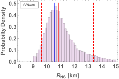
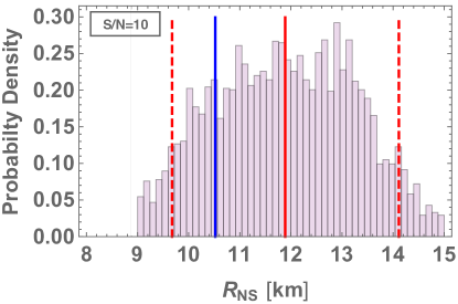
Figure 2: $R_{\rm NS}$ posterior distribution for case m484chi048H at ${\rm\acs{SNR}}=30$ (top panel) and ${\rm\acs{SNR}}=10$ (bottom panel). The red line indicates the median value of the posterior, while the red dashed lines mark the 90% credible interval. The blue line represents the injected value of the radius.

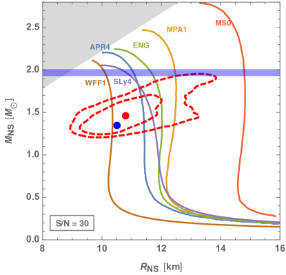
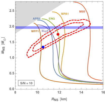
Figure 3: NS mass and radius constraints obtained with our method for case m484chi048H and $\rm{\acs{SNR}}=30$ and $\rm{\acs{SNR}}=10$ in the top and bottom panel, respectively. NS equilibrium sequences for different NS EOSs are also shown. The shaded gray region discards mass-radius combinations excluded by the causality constrain. The horizontal blue band denotes the mass of the high-mass NS J1614-2230 (Demorest et al., 2010). The dashed red lines represent the $68\%$ and $90\%$ credible regions. The blue dot marks the injected mass and radius values, while the red dot denotes the values recovered by the analysis as the median of the mass and radius distributions.

Figure 2 shows the $R_{\rm NS}$ posterior distribution obtained for case m484chi048H (i.e., $M_{\rm BH}=4.84\,M_{\odot}$, $M_{\rm NS}=1.35\,M_{\odot}$, $\chi_{\rm BH}=0.48$, $E_{\gamma,{\rm ISO}}=5\times 10^{51}\,$erg): the top and bottom panel correspond to $\rm{\acs{SNR}}=30$ and $\rm{\acs{SNR}}=10$, respectively. The blue solid line marks the target value of the radius, while the red solid line marks $\lambda$, the median of the posterior. Finally, the red dashed lines mark the 5th and 95th percentiles of the posterior distribution ($\lambda_{-}$, $\lambda_{+}$, with $\lambda_{-}<\lambda_{+}$), which enclose the 90% credible interval. With this choice, the statistical error on the measurement is given by

$$\sigma_{\rm Stat}\equiv\frac{\lambda_{+}-\lambda_{-}}{2\lambda}\,.$$ (9)

We see that the 90% credible interval encloses the target value of $R_{\rm NS}$ and that, as expected, it decreases as the S/N increases. Similarly, the difference between the injected value of $R_{\rm NS}$ and the median of the $R_{\rm NS}$ posterior decreases with increasing S/N. These dependencies on S/N are a sign of the impact that the our GW-informed prior for $M_{\rm NS}$, $M_{\rm BH}$, and $\chi_{\rm BH}$ has on the final results of our approach. We will return to this point in Sec. 3.5.

In Fig. 3, the results for case m484chi048H are displayed in the $M_{\rm NS}$–$R_{\rm NS}$ plane and overlaid on NS equilibrium sequences obtained with the APR4 (Akmal et al., 1998), ENG (Engvik et al., 1996), MPA1 (Müther et al., 1987), MS0 (Müller & Serot, 1996), SLy4 (Chabanat et al., 1998), and WFF1 (Wiringa et al., 1988) NS EOSs. Here the gray shaded area denotes the region of the $M_{\rm NS}-R_{\rm NS}$ plane where the causality constrain is not satisfied, while the blue horizontal band reports the mass of the millisecond pulsar J1614-2230, one of the NSs with the highest mass observed (Demorest et al., 2010). We can see that all the EOSs considered in this figure can account for this high value of mass. The red dashed contours represent the $68\%$ and $90\%$ credible regions. As expected, this region shrinks as the S/N increases, while still including the injected values of mass and radius (blue dot).

Similar results hold for case m484chi048L and are shown in Figures 4 and 5. The decrease in SGRB energy causes the high-end tails of the $R_{\rm NS}$ distribution to be slightly less populated with respect to the m484chi048H case. This is not surprising: powering a more energetic SGRB requires a more massive torus, and lower values of $\epsilon$ can accommodate larger values of $R_{\rm NS}$ in such a scenario. In turn, this means that the impact of the prior on $\epsilon$ progressively increases with the SGRB energy.

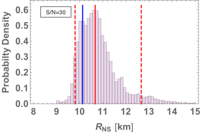
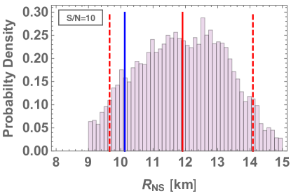
Figure 4: Same as Fig. 2 but for case m484chi048L.

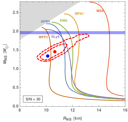
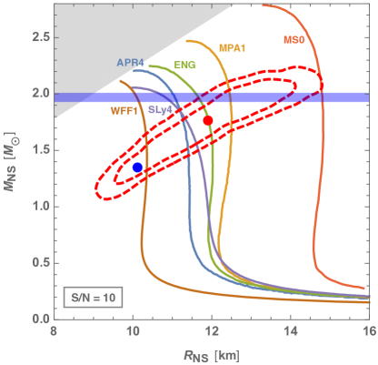
Figure 5: Same as Fig. 3, but for case m484chi048L.

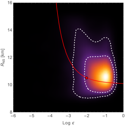
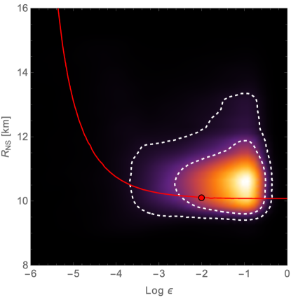
Figure 6: NS radius and mass-energy conversion efficiency $\epsilon$ constraints for case m484chi048H (top panel) and case m484chi048L (bottom panel) with ${\rm\acs{SNR}}=30$. The white dashed curves represents the 68% and 90% credible regions, respectively. The red solid curves are the isoenergetic curve of the injection. The red dot marks the value of the injected epsilon and $R_{\rm NS}$.

This can be further understood from Fig. 6, where the recovered posterior distributions for the high-energy case m484chi048H (top panel) and the low-energy case m484chi048L (bottom panel) are compared in the $\epsilon$–$R_{\rm NS}$ plane at ${\rm\acs{SNR}}=30$. The red dot marks the simulated scenario, while the white, dashed lines denote the 68% and 90% credible regions. In the low-energy case, the distribution is populated in regions with $\epsilon\lesssim 10^{-3}$, so that the overall weight of high $R_{\rm NS}$ values is reduced with respect to the high-energy case. Furthermore, an $\epsilon\lesssim 0.1\%$ gradually becomes unable to accommodate the high-energy scenario, while this is not the case for the low-energy case. Finally, the red line is the curve of constant $E_{\gamma}$ (isoenergetic curve) obtained from Eq. (7) for this specific simulated scenario (i.e., for $M_{\rm BH}=4.84\,M_{\odot}$, $M_{\rm NS}=1.35\,M_{\odot}$, $\chi_{\rm BH}=0.48$, $E_{\gamma,{\rm ISO}}=10^{50}\,$erg, $\theta_{\rm j}\simeq 11^{\circ}$, $c_{2}=17/200$, $\epsilon=0.01$). The fact that this curve cuts through the 68% credible region shows that our analysis is capable of recovering the simulated scenario.

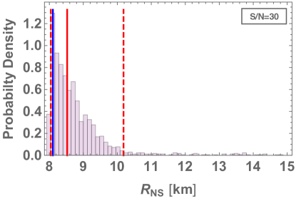
Figure 7: $R_{\rm NS}$ posterior distribution (top panel) with the 68% and 90% credible regions in the $M_{\rm NS}$–$R_{\rm NS}$ plane (bottom panel) for case m484chi080H.

We now vary the injected BH parameters ($M_{\rm BH}$ and $\chi_{\rm BH}$) to see how this affects the recovery of $R_{\rm NS}$. We begin from the BH spin. Figure 7 reports the results at ${\rm\acs{SNR}}=30$ for case m484chi080H. A comparison with the m484chi048H results (Figs. 2 and 3, top panels) highlights that, as the BH spin increases from $\chi_{\rm BH}=0.48$ to $\chi_{\rm BH}=0.8$, the $R_{\rm NS}$ posterior distribution shifts to lower values, correctly following the injected $R_{\rm NS}$ value. In this particular case, where the value of the injected $R_{\rm NS}$ is small (see row 4 in Table 1), results are obtained by extending the prior on $R_{\rm NS}$ down to $8$ km in order to avoid a railing of the posterior distribution against the standard boundary at $9\,$km.

Figure 8 shows the results for case m100chi070H, i.e., the BH has a rather high mass and spin ($M_{\rm BH}=10\,M_{\odot}$, $\chi_{\rm BH}=0.7$). In this case, the BH mass increase requires a higher simulated $R_{\rm NS}$ value, and the $R_{\rm NS}$ posterior distribution accordingly shifts toward higher values.

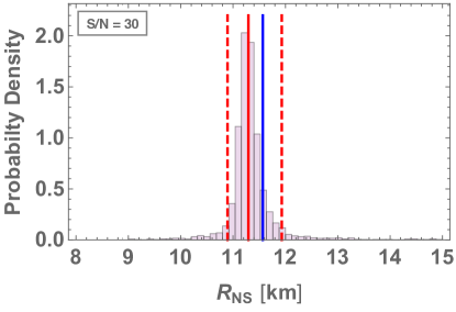
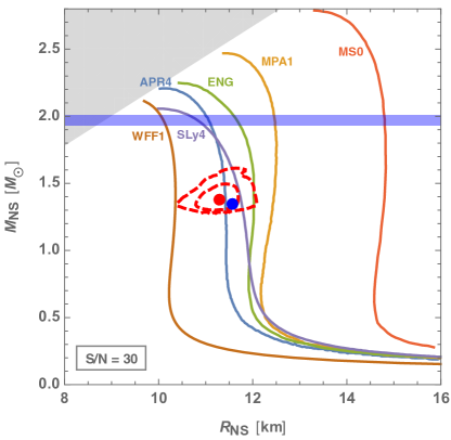
Figure 8: Same as Fig. 7 but for the m100chi070H case.

3.5 Accuracy of the $R_{\rm NS}$ measurement

In this section, we address the impact of the GW posterior, which we use as an informed prior for our method, on the measurement of $R_{\rm NS}$. Furthermore, we discuss the overall uncertainty on the NS radius recovered with our approach.

Figure 9 shows cases m484chi048H and m484chi048L analyzed in the hypothetical scenario in which $M_{\rm BH}$, $M_{\rm NS}$, and $\chi_{\rm BH}$ are known exactly (which makes the S/N value irrelevant). In other words, we set to zero any systematics deriving from the GW informed prior, but we sample $\epsilon$, $\theta_{\rm j}$, and $c_{2}$ normally. This allows us to quantify how the analysis of the GW data influences our final result. The upper and bottom panel of this figure should be compared to the panels in Figs. 2 and 4, respectively. In the high-energy case, the recovered median now slightly underestimates the injected value of $R_{\rm NS}$, and the width of the posterior is reduced. The change in width of the posterior is even more dramatic for the low-energy case, which now displays a virtually perfect recovery of the injected value.

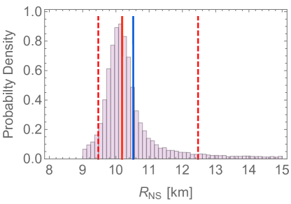
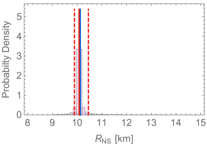
Figure 9: $R_{\rm NS}$ posterior obtained when assuming $M_{\rm NS}$, $M_{\rm BH}$, and $\chi_{\rm BH}$ to be known exactly for cases m484chi048H (top) and m484chi048L (bottom).

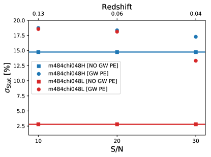
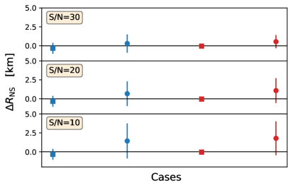
Figure 10: Top panel: statistical error (Eq. (9)) on $R_{\rm NS}$ as function of the GW S/N. The blue and red markers denote cases m484chi048H and m484chi048L, respectively. The circles (squares) represent cases that use (do not use) the prior on $M_{\rm NS}$, $M_{\rm BH}$, and $\chi_{\rm BH}$ informed by GW parameter estimation [which is denoted as “GW PE” in the legend]. Bottom panel: error on $R_{\rm NS}$ for all the scenarios considered in the top panel; the symbols denote the systematic error, that is, the difference between the median and the injected value, while the bars indicate the 90% credible intervals, i.e., the statistical uncertainty.

The top and bottom panels in Fig. 10 show how the statistical error on $R_{\rm NS}$, as defined in Eq. (9), and the systematic error on $R_{\rm NS}$ vary with the S/N of the GW signal for cases m484chi048H (blue) and m484chi048L (red), when using the GW informed prior (circles) and when, instead, assuming that the two masses and the BH spin are known exactly (squares). The statistical error on $R_{\rm NS}$ (top panel) for the m484chi048H and m484chi048L standard analysis setup is well behaved as it decreases with S/N. When we assume $M_{\rm NS}$, $M_{\rm BH}$, and $\chi_{\rm BH}$ to be known exactly, it clearly does not depend on the GW S/N, hence the use of a continuous line at a constant value. The statistical error in the low-energy case is systematically lower than that in the high-energy case. As discussed in Sec. 3.3.1, this happens because the results for the low SGRB energy case depend more weakly on $\epsilon$. Since $\theta_{\rm j}$ and $c_{2}$ enter Eq. (7) in the same term as $\epsilon$, the same argument may be applied to these two parameters. Overall, at lower SGRB energy the impact of $\epsilon$, $\theta_{\rm j}$, and $c_{2}$ on the final result is weaker, which in turn means that the statistical uncertainty on $R_{\rm NS}$ is expected to decrease. As demonstrated in the top panel of Fig. 10, this also implies that within our approach the SGRB energy determines a lower bound on the statistical error on $R_{\rm NS}$ that cannot be beaten by increasing the GW S/N. Furthermore, this bound decreases with the SGRB energy. Therefore, for low energies the uncertainties on $M_{\rm NS}$, $M_{\rm BH}$, and $\chi_{\rm BH}$, which derive solely from the analysis of the GW data, end up dominating the accuracy of the measurement of $R_{\rm NS}$. The bottom panel shows that, unsurprisingly, the bias in the measurement of $R_{\rm NS}$ is larger when using the GW informed prior, as opposed to when $M_{\rm NS}$, $M_{\rm BH}$, and $\chi_{\rm BH}$ are assumed to be known exactly. As expected, the overall bias decreases with S/N. Finally, by contrasting results for which we assume to know the values of $M_{\rm NS}$, $M_{\rm BH}$, and $\chi_{\rm BH}$ (squares) to results that are not based on this assumption (circles), we see that the bias introduced by the GW analysis acts in the direction opposite of that of the bias introduced by the second step of our hierarchical method, i.e., sampling of $\epsilon$, $\theta_{\rm j}$ and $c_{2}$ and use of Eq. (4).

Our lack of knowledge about $\theta_{\rm j}$ and $\epsilon$ contributes in shaping the $R_{\rm NS}$ posterior distribution. Therefore, in the event of a joint GW-SGRB NS-BH observation, any input from additional EM observations and from theoretical studies about jet-launching mechanisms could lead to improvements in the $R_{\rm NS}$ posterior distribution. Similarly, detailed analyses of the GW alone could also improve the radius measurement further by providing a tighter informed prior for $R_{\rm NS}$ (Abbott et al., 2018, 2019).

Finally, we wish to stress that, unfortunately, a proper assessment of all the systematics that enter our method is currently unfeasible. A first assessment of systematics could be achieved as follows. One would have to run numerical-relativity simulations of various NS-BH mergers, extract the remnant masses from them, build complete GW signals by combining analytic approaches for the early inspiral with the numerical data for the late inspiral and merger, and finally test our method against such signals and remnant mass values. This extensive investigation is beyond the scope of the present work and we leave it as a topic for future studies. Because it would heavily rely on numerical-relativity simulations, this would only be a first, albeit significant step. Importantly, in this context, Foucart et al. (2018) found no systematic bias associated with the numerical-relativity code used to determine remnant mass values and that different codes predict remnant masses to within the accuracy of Eq. (4).

4 Discussion

The joint observation of GW170817 and GRB 170817A has unambiguously associated NS-NS coalescences and SGRBs (Abbott et al., 2017b) confirming the long-standing hypothesis that NS-NS binaries are SGRB progenitors (Blinnikov et al., 1984; Eichler et al., 1989; Paczynski, 1986; Eichler et al., 1989; Paczynski, 1991; Narayan et al., 1992). While the rate of NS-NS mergers can accommodate for the rate of observed SGRB events (Abbott et al., 2017b), the question of whether SGRBs have more than one kind of progenitor remains an open one, and one that future observing runs of current and upcoming GW detection facilities will help answer. NS-BH systems, in particular, remain a viable SGRB progenitor candidate (see, e.g., Nakar (2007)). Clark et al. (2015) determine a projected joint GW-SGRB detection rate for NS-BH coalescences of $0.1$–$2\,$yr^-1 for Advanced LIGO and Virgo at design sensitivity and the Fermi Gamma-Ray Burst Monitor, which decreases to $0.03$–$0.7\,\mathrm{yr}^{-1}$ with Swift. Similarly, Regimbau et al. (2015) found a joint GW-SGRB detection rate with Swift of $0.05$–$0.06\,\mathrm{yr^{-1}}$ while Wanderman & Piran (2015) found $0.4$–$1\,\mathrm{yr^{-1}}$ ($3$–$6\,\mathrm{yr^{-1}}$ with Fermi Gamma-Ray Burst Monitor). The next generation of GW interferometers will extend the NS-BH detection horizon up to $z\simeq 4$ (Abernathy et al., 2011) therefore boosting such detection rates.

In this paper, we presented a method based on Pannarale & Ohme (2014) to exploit joint GW-SGRB observations of NS-BH coalescences in order to measure the NS radius, and hence, constrain the EOS of matter at supranuclear densities. We sample the GW posterior distribution of the component masses and the BH spin along with uniform prior distributions on other unknown physical parameters involved in the problem — among which is the NS radius (see Sec. 2 for details) — and determine a distribution of isotropic gamma-ray energies. This is then combined with the EM measurement of the isotropic gamma-ray energy to yield a constraint on the NS radius, after marginalizing over all other sampled quantities. Hinderer et al. (2018) performed a similar analysis on GW170817, also using Foucart et al. (2018) and working under the assumption that the event originated from a NS-BH coalescence, but exploiting the EM constraints from the kilonova light curve, rather than the SGRB energy.

In order to test the performance and the robustness of our method, we simulated six joint GW-SGRB NS-BH detection scenarios (see Table 1). In each case, we compared the injected $R_{\rm NS}$ value to the posterior distribution recovered by our analysis. While this setup does not allow us to assess systematics in our methodology (see the discussion at the end of Sec. 3.5), it is currently the only possible benchmark and it allows us to draw the following first, important conclusions about our method:

• The 90% credible regions we determine always contains the injected value of $R_{\rm NS}$, regardless of the mass and/or spin of the BH in the NS-BH system under consideration.

• With the exception of case m100chi070H, the median of the $R_{\rm NS}$ posterior distribution is usually higher than the injected NS value and it is narrower for lower-energy SGRBs (i.e., $E_{\gamma,{\rm ISO}}\lesssim 10^{50}\,$erg).

• We can constrain the NS radius with an uncertainty (quantified from a 90% of credible interval) below 20% even for low S/N events.

• The $R_{\rm NS}$ lower bound is rather solid and depends mostly on the S/N of the GW signal through the informed prior for the GW parameters.

• By directly sampling the posterior distributions of GW parameter estimation analyses, our method inherits any uncertainty that is present in such distributions. This component of the overall error on the recovered $R_{\rm NS}$ reduces as the S/N of the GW increases. However, in Sec. 3.5 we showed that the SGRB energy determines a hard lower limit for the uncertainty on $R_{\rm NS}$. The value of this contribution to the overall error is clearly S/N independent, but it decreases with the SGRB energy. For example, for the source configuration considered in Fig. 10, this lower limit varies from $\sim 3\%$ to $\sim 15\%$ as $E_{\gamma,{\rm ISO}}$ goes from $10^{50}\,\rm erg/s$ to $5\times 10^{51}\,\rm erg/s$.

A central ingredient of our method is the fitting formula that predicts the mass of the matter that remains in the surroundings of the remnant BH immediately after the merger as a function of the NS-BH initial parameters (Foucart et al., 2018). This can be replaced as improved or different versions of such formula are published. However, as long as it remains the only available option in the literature, a study of systematics continues to be a time and resource intensive task that would essentially require a campaign of numerical-relativity simulations (see discussion at the end of Sec. 3.5). Furthermore, for such a study to be fully self-consistent, one would require simulations that evolve the NS-BH system all the way from inspiral to the ignition of the SGRB. For the time being, the tolerance we introduce in Eq. (6) when comparing our inferred $E_{\gamma,{\rm ISO}}$ values to the observed $E_{\gamma,{\rm ISO}}$ accounts for systematic uncertainties in the fit of Foucart et al. (2018), but also for possible differences between the remnant mass that it models and the disk mass that actually accretes onto the central BH. These two quantities may differ, for instance, if a non-negligible fraction of remnant mass were to be lost in form of dynamical ejecta or disk winds (Kawaguchi et al., 2016). Although our method is therefore model-dependent, we note that this is a shared feature of all other existing methods to measure NS radii (for a recent review, see Özel & Freire (2016)). For example, $R_{\rm NS}$ constraints from low-mass X-ray binary observations that are based on spectroscopic measurements of such sources in a quiescent state (Heinke et al., 2006; Webb & Barret, 2007; Guillot et al., 2011; Bogdanov et al., 2016) or after a thermonuclear burst (van Paradijs, 1979; Özel et al., 2009; Güver et al., 2010b, a; Özel et al., 2012; Güver & Özel, 2013) require, among other things, introducing assumptions about the NS atmosphere composition and magnetic field. Other methods that involve timing measurements of oscillations in accretion-powered pulsars (Poutanen & Gierliński, 2003; Leahy et al., 2008, 2009, 2011; Morsink & Leahy, 2011) require modeling the pulsed waveform and therefore depend on assumptions about NS spacetimes and other geometrical factors, such as the shape and location of the surface hotspots. Finally, EOS constraints that rely on the analysis of GW data, including our method, intrinsically depend on the waveform models used to process the GW data and on how these treat tidal effects (Abbott et al., 2018, 2019). These examples illustrate that a model dependency is unavoidable when addressing the task of measuring NS radii. However, the availability of a number of methods each one of which relies on different assumptions and on the observation of different astrophysical systems is crucial: the combination of results that stem from various approaches can provide a more solid, final result.

On the basis of the work carried out in this paper, there are a number of lines of investigation that we plan to explore. Firstly, in the event of an NS-BH detection, a detailed analysis of the GW that constrains the NS tidal deformability would be carried out, as was the case for the NS-NS coalescence event GW170817 (Abbott et al., 2017f, 2018, 2019). In turn, this information and the so-called “universal relations” (see, e.g., Yagi & Yunes (2017) for a review) could be exploited to build a less agnostic sampling of the NS radius to be used within our approach (currently a uniform prior between $9\,$ and $15\,$km): upper limits on the tidal deformability would result in a narrower interval to be sampled. Moreover, this informed prior on $R_{\rm NS}$ would also ensure a more consistent sampling of the NS mass and radius, with more massive objects associated with higher compactnesses. Furthermore, in the event of an NS-BH merger observation in which the NS is disrupted by the BH tidal field, the GW signal is expected to shut off at a characteristic frequency which depends, among other things, on the NS EOS (Shibata et al., 2009; Kyutoku et al., 2011; Pannarale et al., 2015b). The measurement of this frequency would yield constraints on $R_{\rm NS}$ with a $10$–$40$% accuracy (Lackey et al., 2012, 2014), and we want to assess the impact of including such information into our analysis. This scenario is particularly relevant for third-generation GW detectors because the shutoff of NS-BH signals happens in the $\sim$kHz GW frequency regime. The projected NS-BH detection rate for the Einstein Telescope is $\mathcal{O}(10^{3}$–$10^{7}\,$yr${}^{-1})$ (Abernathy et al., 2011). In order to guarantee a high-joint GW-SGRB detection rate of such events and to unleash the full potential they have to constrain the NS EOS, it will be of paramount importance to have functioning high-energy gamma-ray observing facilities during the lifespan of third-generation GW detectors. Finally, other independent constraints that would reduce our prior on $R_{\rm NS}$ are expected to result from ongoing and future missions such as NICER (Arzoumanian et al., 2014), ATHENA (Motch et al., 2013), and eXTP (Zhang et al., 2016).

Label	S/N	$M_{\rm NS}$	$M_{\rm BH}$	$\chi_{\rm BH}$	$\rm q$
		$[M_{\odot}]$	$[M_{\odot}]$
m484chi048(H/L)	10	1.25 - 2.46	2.57 - 5.47	0.14 - 0.81	1.05 - 4.31
	30	1.28 - 1.94	3.19 - 5.26	0.23 - 0.68	1.64 - 4.11
m484chi080(H/L)	30	1.19 - 2.29	2.66 - 5.72	0.65 - 0.88	1.16 - 4.79
m100chi070(H/L)	30	1.32 - 1.56	8.30 - 10.44	0.67 - 0.76	5.32 - 7.89

Table A.2: 90% credible intervals of binary system properties obtained by the parameter estimation of the GW signal injections used in our study.

Label	S/N	$M_{\rm NS}$	$M_{\rm BH}$	$\chi_{\rm BH}$	$\rm q$
		$[M_{\odot}]$	$[M_{\odot}]$
m484chi048(H/L)	10	1.20 - 2.12	2.57 - 5.47	0.14 - 0.81	1.45 - 4.83
	30	1.29 - 1.83	3.05 - 5.84	0.38 - 0.68	1.86 - 4.07
m484chi080(H/L)	30	1.13 - 1.89	3.30 - 6.17	0.76 - 0.88	1.74 - 5.46
m100chi070(H/L)	30	1.32 - 1.53	8.52 - 10.46	0.68 - 0.72	5.56 - 7.90

Table A.3: Same as Table A.2, but obtained from the posterior probability distribution after it is pruned in order to select only parameters compatible with NS-BH systems.

References

- Aasi et al. (2015a) Aasi, J., et al. 2015a, Class. Quant. Grav., 32, 074001
- Aasi et al. (2015b) —. 2015b, Class. Quantum Grav., 32, 074001
- Abbott et al. (2013) Abbott, B. P., et al. 2013, arXiv:1304.0670, [Living Rev. Rel.19,1(2016)]
- Abbott et al. (2016a) —. 2016a, Phys. Rev. Lett., 116, 241103
- Abbott et al. (2016b) —. 2016b, Phys. Rev. Lett., 116, 061102
- Abbott et al. (2017a) —. 2017a, Astrophys. J., 850, L39
- Abbott et al. (2017b) —. 2017b, Astrophys. J., 848, L13
- Abbott et al. (2017c) —. 2017c, Phys. Rev. Lett., 118, 221101
- Abbott et al. (2017d) —. 2017d, Astrophys. J., 851, L35
- Abbott et al. (2017e) —. 2017e, Phys. Rev. Lett., 119, 141101
- Abbott et al. (2017f) —. 2017f, Phys. Rev. Lett., 119, 161101
- Abbott et al. (2017g) —. 2017g, Astrophys. J., 848, L12
- Abbott et al. (2018) Abbott, B. P., Abbott, R., Abbott, T. D., et al. 2018, Physical Review Letters, 121, 161101
- Abbott et al. (2018) Abbott, B. P., et al. 2018, arXiv:1811.12907
- Abbott et al. (2019) Abbott, B. P., Abbott, R., Abbott, T. D., et al. 2019, Physical Review X, 9, 011001
- Abernathy et al. (2011) Abernathy, M., et al. 2011, Einstein gravitational wave Telescope conceptual design study. ET-0106C-10, https://tds.ego-gw.it/ql/?c=7954, ,
- Acernese et al. (2015) Acernese, F., et al. 2015, Class. Quant. Grav., 32, 024001
- Akmal et al. (1998) Akmal, A., Pandharipande, V. R., & Ravenhall, D. G. 1998, PhRvC, 58, 1804
- Arzoumanian et al. (2014) Arzoumanian, Z., Gendreau, K. C., Baker, C. L., et al. 2014, in Proc. SPIE, Vol. 9144, Space Telescopes and Instrumentation 2014: Ultraviolet to Gamma Ray, 914420
- Aso et al. (2013) Aso, Y., Michimura, Y., Somiya, K., et al. 2013, Phys. Rev., D88, 043007
- Bardeen et al. (1972) Bardeen, J. M., Press, W. H., & Teukolsky, S. A. 1972, Astrophys. J., 178, 347
- Berger (2014) Berger, E. 2014, ARA&A, 52, 43
- Bildsten & Cutler (1992) Bildsten, L., & Cutler, C. 1992, ApJ, 400, 175
- Blandford & Payne (1982) Blandford, R. D., & Payne, D. G. 1982, MNRAS, 199, 883
- Blandford & Znajek (1977) Blandford, R. D., & Znajek, R. L. 1977, MNRAS, 179, 433
- Blinnikov et al. (1984) Blinnikov, S. I., Novikov, I. D., Perevodchikova, T. V., & Polnarev, A. G. 1984, SvAL, 10, 177
- Bogdanov et al. (2016) Bogdanov, S., Heinke, C. O., Özel, F., & Güver, T. 2016, ApJ, 831, 184
- Chabanat et al. (1998) Chabanat, E., Bonche, P., Haensel, P., Meyer, J., & Schaeffer, R. 1998, Nuclear Physics A, 635, 231
- Cipolletta et al. (2015) Cipolletta, F., Cherubini, C., Filippi, S., Rueda, J. A., & Ruffini, R. 2015, Phys. Rev. D, 92, 023007
- Clark et al. (2015) Clark, J., Evans, H., Fairhurst, S., et al. 2015, Astrophys. J., 809, 53
- Demorest et al. (2010) Demorest, P. B., Pennucci, T., Ransom, S. M., Roberts, M. S. E., & Hessels, J. W. T. 2010, Nature, 467, 1081
- Dietrich et al. (2018) Dietrich, T., Khan, S., Dudi, R., et al. 2018, ArXiv e-prints, arXiv:1804.02235
- Duez et al. (2010) Duez, M. D., Foucart, F., Kidder, L. E., Ott, C. D., & Teukolsky, S. A. 2010, Classical and Quantum Gravity, 27, 114106
- Eichler et al. (1989) Eichler, D., Livio, M., Piran, T., & Schramm, D. N. 1989, Nature, 340, 126
- Engvik et al. (1996) Engvik, L., Osnes, E., Hjorth-Jensen, M., Bao, G., & Ostgaard, E. 1996, ApJ, 469, 794
- Fairhurst (2018) Fairhurst, S. 2018, Class. Quant. Grav., 35, 105002
- Fernández & Metzger (2016) Fernández, R., & Metzger, B. D. 2016, Ann. Rev. Nucl. Part. Sci., 66, 23
- Foucart (2012) Foucart, F. 2012, PhRvD, 86, 124007
- Foucart et al. (2018) Foucart, F., Hinderer, T., & Nissanke, S. 2018, ArXiv e-prints, arXiv:1807.00011
- Foucart et al. (2013) Foucart, F., Deaton, M. B., Duez, M. D., et al. 2013, Phys. Rev., D87, 084006
- Foucart et al. (2014) —. 2014, Phys. Rev., D90, 024026
- Foucart et al. (2017) Foucart, F., Desai, D., Brege, W., et al. 2017, Classical and Quantum Gravity, 34, 044002
- Giacomazzo et al. (2013) Giacomazzo, B., Perna, R., Rezzolla, L., Troja, E., & Lazzati, D. 2013, ApJ, 762, L18
- Glendenning (1992) Glendenning, N. K. 1992, Phys. Rev. D, 46, 1274
- Guillot et al. (2011) Guillot, S., Rutledge, R. E., & Brown, E. F. 2011, ApJ, 732, 88
- Güver & Özel (2013) Güver, T., & Özel, F. 2013, ApJ, 765, L1
- Güver et al. (2010a) Güver, T., Özel, F., Cabrera-Lavers, A., & Wroblewski, P. 2010a, ApJ, 712, 964
- Güver et al. (2010b) Güver, T., Wroblewski, P., Camarota, L., & Özel, F. 2010b, ApJ, 719, 1807
- Hannam et al. (2014) Hannam, M., Schmidt, P., Bohé, A., et al. 2014, Phys. Rev. Lett., 113, 151101
- Hawley & Krolik (2006) Hawley, J. F., & Krolik, J. H. 2006, ApJ, 641, 103
- Heinke et al. (2006) Heinke, C. O., Rybicki, G. B., Narayan, R., & Grindlay, J. E. 2006, ApJ, 644, 1090
- Hinderer et al. (2016) Hinderer, T., Taracchini, A., Foucart, F., et al. 2016, Physical Review Letters, 116, 181101
- Hinderer et al. (2018) Hinderer, T., Nissanke, S., Foucart, F., et al. 2018, Discerning the binary neutron star or neutron star-black hole nature of GW170817 with Gravitational Wave and Electromagnetic Measurements, (in preparation), ,
- Husa et al. (2016) Husa, S., Khan, S., Hannam, M., et al. 2016, Phys. Rev. D, 93, 044006
- Iyer et al. (2011) Iyer, B., et al. 2011, LIGO India, Tech. Rep. LIGO-M1100296, https://dcc.ligo.org/LIGO-M1100296/public
- Kalogera et al. (2019) Kalogera, V., et al. 2019, arXiv:1903.09220
- Kawaguchi et al. (2015) Kawaguchi, K., Kyutoku, K., Nakano, H., et al. 2015, Phys. Rev., D92, 024014
- Kawaguchi et al. (2016) Kawaguchi, K., Kyutoku, K., Shibata, M., & Tanaka, M. 2016, ApJ, 825, 52
- Kawaguchi et al. (2016) Kawaguchi, K., Kyutoku, K., Shibata, M., & Tanaka, M. 2016, Astrophys. J., 825, 52
- Khan et al. (2016) Khan, S., Husa, S., Hannam, M., et al. 2016, Phys. Rev. D, 93, 044007
- Kokkotas & Schafer (1995) Kokkotas, K. D., & Schafer, G. 1995, MNRAS, 275, 301
- Kulkarni (2005) Kulkarni, S. R. 2005, arXiv:astro-ph/0510256
- Kumar et al. (2017) Kumar, P., Pürrer, M., & Pfeiffer, H. P. 2017, Phys. Rev. D, 95, 044039
- Kyutoku et al. (2015) Kyutoku, K., Ioka, K., Okawa, H., Shibata, M., & Taniguchi, K. 2015, Phys. Rev. D, 92, 044028
- Kyutoku et al. (2011) Kyutoku, K., Okawa, H., Shibata, M., & Taniguchi, K. 2011, Phys. Rev. D, 84, 064018
- Kyutoku et al. (2010) Kyutoku, K., Shibata, M., & Taniguchi, K. 2010, PhRvD, 82, 044049
- Lackey et al. (2012) Lackey, B. D., Kyutoku, K., Shibata, M., Brady, P. R., & Friedman, J. L. 2012, PhRvD, 85, 044061
- Lackey et al. (2014) —. 2014, Phys. Rev. D, 89, 043009
- Lattimer & Prakash (2016) Lattimer, J. M., & Prakash, M. 2016, Phys. Rep., 621, 127
- Lattimer et al. (1990) Lattimer, J. M., Prakash, M., Masak, D., & Yahil, A. 1990, ApJ, 355, 241
- Leahy et al. (2008) Leahy, D. A., Morsink, S. M., & Cadeau, C. 2008, ApJ, 672, 1119
- Leahy et al. (2011) Leahy, D. A., Morsink, S. M., & Chou, Y. 2011, ApJ, 742, 17
- Leahy et al. (2009) Leahy, D. A., Morsink, S. M., Chung, Y.-Y., & Chou, Y. 2009, ApJ, 691, 1235
- Lee & Ramirez-Ruiz (2007) Lee, W. H., & Ramirez-Ruiz, E. 2007, New Journal of Physics, 9, 17
- Li & Paczyński (1998) Li, L.-X., & Paczyński, B. 1998, ApJ, 507, L59
-
LIGO Scientific Collaboration, Virgo
Collaboration (2017)
LIGO Scientific Collaboration, Virgo Collaboration. 2017,
LALSuite,
https://git.ligo.org/lscsoft/lalsuite/
tree/lalinference_o2, GitLab - Mészáros (2006) Mészáros, P. 2006, Reports on Progress in Physics, 69, 2259
- Meszaros & Rees (1992) Meszaros, P., & Rees, M. J. 1992, Astrophys. J., 397, 570
- Metzger (2017) Metzger, B. D. 2017, Living Reviews in Relativity, 20, 3
- Metzger & Berger (2012) Metzger, B. D., & Berger, E. 2012, ApJ, 746, 48
- Metzger et al. (2010) Metzger, B. D., Martínez-Pinedo, G., Darbha, S., et al. 2010, Monthly Notices of the Royal Astronomical Society, 406, 2650
- Morsink & Leahy (2011) Morsink, S. M., & Leahy, D. A. 2011, ApJ, 726, 56
- Motch et al. (2013) Motch, C., et al. 2013, arXiv:1306.2334
- Müller & Serot (1996) Müller, H., & Serot, B. D. 1996, Nuclear Physics A, 606, 508
- Müther et al. (1987) Müther, H., Prakash, M., & Ainsworth, T. L. 1987, Physics Letters B, 199, 469
- Nakar (2007) Nakar, E. 2007, PhR, 442, 166
- Narayan et al. (1992) Narayan, R., Paczynski, B., & Piran, T. 1992, ApJ, 395, L83
- Nissanke et al. (2013) Nissanke, S., Kasliwal, M., & Georgieva, A. 2013, Astrophys. J., 767, 124
- Oppenheimer & Volkoff (1939) Oppenheimer, J. R., & Volkoff, G. M. 1939, Physical Review, 55, 374
- Özel & Freire (2016) Özel, F., & Freire, P. 2016, ARA&A, 54, 401
- Özel et al. (2012) Özel, F., Gould, A., & Güver, T. 2012, ApJ, 748, 5
- Özel et al. (2009) Özel, F., Güver, T., & Psaltis, D. 2009, ApJ, 693, 1775
- Paczynski (1986) Paczynski, B. 1986, ApJ, 308, L43
- Paczynski (1991) —. 1991, Acta Astron., 41, 257
- Pannarale et al. (2015a) Pannarale, F., Berti, E., Kyutoku, K., Lackey, B. D., & Shibata, M. 2015a, Phys. Rev., D92, 084050
- Pannarale et al. (2015b) —. 2015b, Phys. Rev., D92, 081504
- Pannarale et al. (2013) Pannarale, F., Berti, E., Kyutoku, K., & Shibata, M. 2013, Phys. Rev., D88, 084011
- Pannarale & Ohme (2014) Pannarale, F., & Ohme, F. 2014, Astrophys. J., 791, L7
- Pannarale et al. (2011) Pannarale, F., Rezzolla, L., Ohme, F., & Read, J. S. 2011, Phys. Rev. D, 84, 104017
- Pannarale et al. (2011) Pannarale, F., Tonita, A., & Rezzolla, L. 2011, ApJ, 727, 95
- Parfrey et al. (2015) Parfrey, K., Giannios, D., & Beloborodov, A. M. 2015, MNRAS, 446, L61
- Poutanen & Gierliński (2003) Poutanen, J., & Gierliński, M. 2003, MNRAS, 343, 1301
- Punturo et al. (2010) Punturo, M., et al. 2010, Class. Quant. Grav., 27, 194002
- Regimbau et al. (2015) Regimbau, T., Siellez, K., Meacher, D., Gendre, B., & Boër, M. 2015, Astrophys. J., 799, 69
- Sari et al. (1999) Sari, R., Piran, T., & Halpern, J. P. 1999, ApJ, 519, L17
- Sathyaprakash et al. (2019) Sathyaprakash, B. S., et al. 2019, arXiv:1903.09277
- Setiawan et al. (2004) Setiawan, S., Ruffert, M., & Janka, H.-T. 2004, MNRAS, 352, 753
- Shibata et al. (2009) Shibata, M., Kyutoku, K., Yamamoto, T., & Taniguchi, K. 2009, Phys. Rev., D79, 044030, [Erratum: Phys. Rev.D85,127502(2012)]
- Smith et al. (2016) Smith, R., Field, S. E., Blackburn, K., et al. 2016, Phys. Rev. D, 94, 044031
- Tolman (1939) Tolman, R. C. 1939, Physical Review, 55, 364
- Unnikrishnan (2013) Unnikrishnan, C. S. 2013, Int. J. Mod. Phys., D22, 1341010
- Vallisneri (2000) Vallisneri, M. 2000, Physical Review Letters, 84, 3519
- van Paradijs (1979) van Paradijs, J. 1979, ApJ, 234, 609
- Veitch et al. (2015) Veitch, J., Raymond, V., Farr, B., et al. 2015, Phys. Rev. D, 91, 042003
- Wanderman & Piran (2015) Wanderman, D., & Piran, T. 2015, Mon. Not. Roy. Astron. Soc., 448, 3026
- Webb & Barret (2007) Webb, N. A., & Barret, D. 2007, ApJ, 671, 727
- Wiringa et al. (1988) Wiringa, R. B., Fiks, V., & Fabrocini, A. 1988, Phys. Rev. C, 38, 1010
- Yagi & Yunes (2017) Yagi, K., & Yunes, N. 2017, Phys. Rep., 681, 1
- Zalamea & Beloborodov (2011) Zalamea, I., & Beloborodov, A. M. 2011, MNRAS, 410, 2302
- Zhang et al. (2007) Zhang, B., Liang, E., Page, K. L., et al. 2007, ApJ, 655, 989
- Zhang et al. (2016) Zhang, S. N., et al. 2016, Proc. SPIE Int. Soc. Opt. Eng., 9905, 99051Q