Hyperfine structure of $S$-states in muonic ions of lithium, beryllium and boron.

Abstract

We make precise calculation of hyperfine structure of $S$-states in muonic ions of lithium, beryllium and boron in quantum electrodynamics. Corrections of orders $\alpha^{5}$ and $\alpha^{6}$ due to the vacuum polarization, nuclear structure and recoil in first and second orders of perturbation theory are taken into account. We obtain estimates of the total values of hyperfine splittings which can be used for a comparison with future experimental data.

I Introduction

The hyperfine splitting (HFS) of 2S-state in muonic hydrogen was measured recently by the CREMA collaboration in crema1 :

$$\Delta E^{hfs}_{exp}(2S)=22.8089(51)~{}meV.$$ (1)

The theoretical value of the HFS of 2S-level, which was calculated with high accuracy as a result of taking into account numerous corrections for the vacuum polarization, structure and recoil of the nucleus, relativism agrees well with the value (1). At present, several experimental groups plan to measure the HFS of the ground state in muonic hydrogen with a record accuracy of 1 ppm. This will allow us to better study effects of the structure and polarizability of the proton. Since measurements have already been made of certain transition frequencies $(2P-2S)$ in muonic deuterium and muonic helium ion crema2 ; crema3 ; crema4 , it will apparently allow the experimental value of the HFS of 2S-state to be obtained in the near future for these muonic atoms.

The CREMA collaboration has obtained in recent years significantly new experimental results that helped to re-examine the problem of muon bound states, posed new questions to the theory that require additional investigation. One possible future activity of the CREMA collaboration may be connected with other muonic ions containing light nuclei of lithium, beryllium and boron. For these muonic ions, the description of the electromagnetic interaction of the few-nucleon systems is particularly important, and, consequently, the role of the effects of nuclear physics can be studied with greater accuracy. We may hope that the enormous interest, which experimental results of the CREMA collaboration have met over the past years can ultimately lead to a significant improvement in the theory of calculating the energy levels of muonic atoms.

In our previous work, we calculated the Lamb shift in the muonic ions of lithium, beryllium, and boron apm2016 . The purpose of this paper is to investigate the HFS of the S-states in these ions, that is, in the precise calculation of various corrections and obtaining reliable estimates for the HFS intervals, which could be used for comparison with experimental data. It should be noted that estimates of a number of important contributions to the HFS of ions have already been made in drake . The initial parameters that determine the values of the corrections in the HFS of muonic ions, are the masses of the nuclei, their spins, magnetic moments and charge radii. Since we calculate the corrections immediately for several nuclei, their parameters are presented in a separate Table 1 stone ; marinova .

A part of the Breit Hamiltonian, responsible for hyperfine splitting, has a known form in the coordinate representation:

$$\Delta V_{B}^{hfs}(r)=\frac{4\pi\alpha(1+a_{\mu})\mu_{N}}{3m_{1}m_{p}s_{2}}({\bf s}_{1}{\bf s}_{2})\delta({\bf r}),$$ (2)

where the masses of the muon and nuclear will be denoted further $m_{1}$, $m_{2}$, $m_{p}$ is the proton mass, $\mu_{N}$ is the nuclear magnetic moment in nuclear magnetons, $a_{\mu}$ is the muon anomalous magnetic moment (AMM), ${\bf s}_{1}$ and ${\bf s}_{2}$ are the spins of a muon and nucleus. The potential $\Delta V_{B}^{hfs}$ gives the main part of hyperfine splitting of order $\alpha^{4}$ which is called the Fermi energy:

$$E_{F}(nS)=\frac{2Z^{3}\alpha^{4}\mu^{3}\mu_{N}}{3m_{1}m_{p}n^{3}s_{2}}(2s_{2}+1),$$ (3)

where $n$ is the principal quantum number, $\mu=m_{1}m_{2}/(m_{1}+m_{2})$. The factor $Z^{3}$ ($Z$ is the charge of the nucleus in units of the electron charge) in (3) leads to essential increase of numerical values $E_{F}(nS)$ for the muonic ions of lithium, beryllium and boron in comparison with muonic hydrogen. The muon AMM $a_{\mu}$ is not included in (3).

Table 1: The nucleus parameters of lithium, beryllium and boron.

Nucleus	Spin	Mass ,	Magnetic dipole	Charge radius,	Electroquadrupole	Magnetic octupole
		GeV	moment, nm	fm	moment, fm2	moment, nm$\cdot$fm2
${}^{6}_{3}Li$	1	5.60152	0.8220473(6)	$2.5890\pm 0.0390$	-0.083(8)	0
${}^{7}_{3}Li$	3/2	6.53383	3.256427(2)	$2.4440\pm 0.0420$	-4.06(8)	7.5
${}^{9}_{4}Be$	3/2	8.39479	-1.177432(3)	$2.5190\pm 0.0120$	5.29(4)	4.1
${}^{10}_{5}B$	3	9.32699	0.8220473(6)	$2.4277\pm 0.0499$	8.47(6)	0
${}^{11}_{5}B$	3/2	10.25510	0.8220473(6)	$2.4060\pm 0.0294$	4.07(3)	7.8

The Fermi energy is obtained after averaging (2) over the Coulomb wave functions. In the case of $1S$- and $2S$-states they have the form:

$$\psi_{100}(r)=\frac{W^{3/2}}{\sqrt{\pi}}e^{-Wr},~{}~{}~{}W=\mu Z\alpha,$$ (4)

$$\psi_{200}(r)=\frac{W^{3/2}}{2\sqrt{2\pi}}e^{-Wr/2}\left(1-\frac{Wr}{2}\right).$$ (5)

The muon AMM correction to hyperfine splitting is presented separately in Tables 2-4 (line 2) taking experimental value of muon AMM MT :

$$\Delta E^{hfs}_{a_{\mu}}(nS)=a_{\mu}E_{F}(nS).$$ (6)

Numerical value of relativistic correction of order $\alpha^{6}$ to HFS can be obtained by means of known analytical expression from egs ; breit :

$$\Delta E^{hfs}_{rel}(nS)=\Biggl{\{}{{\frac{3}{2}(Z\alpha)^{2}E_{F}(1S)}\atop{\frac{17}{8}(Z\alpha)^{2}E_{F}(2S)}}.$$ (7)

Next, we investigate a number of basic corrections to the hyperfine structure of $S$-states in order to obtain acceptable total result. Numerical values of different corrections are presented for definiteness with the accuracy $10^{-2}$ meV.

Table 2: Hyperfine splittings of S-states in muonic ions $(\mu~{}^{6}_{3}Li)^{2+}$ and $(\mu~{}^{7}_{3}Li)^{2+}$.

No.	Contribution to the splitting	$(\mu~{}^{6}_{3}Li)^{2+}$, meV		$(\mu~{}^{7}_{3}Li)^{2+}$, meV
		1S	2S	1S	2S
1	Contribution of order $\alpha^{4}$,	1416.07	177.01	5026.00	628.25
	the Fermi energy
2	Muon AMM contribution	1.65	0.21	5.87	0.73
3	Relativistic correction	1.02	0.18	3.62	0.64
	of order $\alpha^{6}$
4	Nuclear structure correction	G; -109.92	G: -13.74	G: -369.25	G: -46.16
	of order $\alpha^{5}$	U: -112.02	U: -14.00	U: -376.31	U: -47.04
5	Nuclear structure and recoil	G: -0.20	G: -0.03	G: -30.67	G: -3.83
6	Nuclear structure correction	3.35	0.34	10.67	1.08
	of order $\alpha^{6}$ in $1\gamma$ interaction
7	Nuclear structure correction in second	-2.56	-0.90	-8.19	-2.90
	order perturbation theory
8	Vacuum polarization contribution	5.22	0.67	18.54	2.38
	of order $\alpha^{5}$ in first order PT
9	Vacuum polarization contribution	12.05	1.11	42.83	3.94
	of order $\alpha^{5}$ in second order PT
10	Muon vacuum polarization contribution	0.08	0.01	0.29	0.04
	of order $\alpha^{6}$ in first order PT
11	Muon vacuum polarization contribution	0.09	0.01	0.31	0.04
	of order $\alpha^{6}$ in second order PT
12	Vacuum polarization contribution	0.07	0.01	0.24	0.03
	of order $\alpha^{6}$ in first order PT
13	Vacuum polarization contribution	0.14	0.02	0.53	0.05
	of order $\alpha^{6}$ in second order PT
14	Nuclear structure and vacuum	-1.62	-0.20	-5.85	-0.73
	polarization correction of order $\alpha^{6}$
15	Nuclear structure and muon vacuum	-0.14	-0.02	-0.51	-0.06
	polarization correction of order $\alpha^{6}$
16	Hadron vacuum polarization	0.06	0.01	0.21	0.03
	contribution of order $\alpha^{6}$
17	Radiative nuclear finite size	-0.34	-0.04	-1.24	-0.15
	correction of order $\alpha^{6}$
	Summary contribution	1325.02	164.65	4693.40	583.38

II Nuclear structure and recoil corrections

When calculating various corrections in the hyperfine structure of the spectrum, it is important to note the essential role of corrections for the structure of the Li, Be, and B nuclei. Such corrections are determined by the electromagnetic form factors of the nuclei. Among the nuclei that we are considering, several nuclei have a spin $s_{2}=3/2$. The amplitude of the one-photon interaction of such nuclei with a muon can be written in the form spin321 ; spin322 ; spin323 :

$$iM_{1\gamma}=-\frac{Ze^{2}}{k^{2}}[\bar{u}(q_{1})\gamma_{\mu}u(p_{1})][\bar{v}_{\alpha}(p_{2}){\cal O}_{\alpha\mu\beta}v_{\beta}(q_{2})]=$$ (8)

$$-\frac{Ze^{2}}{k^{2}}[\bar{u}(q_{1})\gamma_{\mu}u(p_{1})]\bar{v}_{\alpha}(p_{2})\bigl{\{}g_{\alpha\beta}\frac{(p_{2}+q_{2})_{\mu}}{2m_{2}}F_{1}(k^{2})-g_{\alpha\beta}\sigma_{\mu\nu}\frac{k^{\nu}}{2m_{2}}F_{2}(k^{2})+$$

$$\frac{k_{\alpha}k_{\beta}}{4m_{2}^{2}}\frac{(p_{2}+q_{2})_{\mu}}{2m_{2}}F_{3}(k^{2})-\frac{k_{\alpha}k_{\beta}}{4m_{2}^{2}}\sigma_{\mu\nu}\frac{k^{\nu}}{2m_{2}}F_{4}(k^{2})\bigr{\}}v_{\beta}(q_{2}),$$

where $p_{1}$, $p_{2}$ are four-momenta of particles in the initial state, $q_{1}$, $q_{2}$ are four-momenta of particles in the final state, $k=q_{2}-p_{2}=p_{1}-q_{1}$. ${\cal O}_{\alpha\mu\beta}$ is the vertex function of the spin 3/2 nucleus. Nuclei with a spin 3/2 are described by the spin-vector $v_{\alpha}(p)$. Four form factors $F_{i}(k^{2})$ are related to the charge $G_{E0}$, electroquadrupole $G_{E2}$, magnetic dipole $G_{M1}$ and magnetic octupole $G_{M3}$ form factors by the following expressions spin321 ; spin322 ; spin323 :

$$G_{E0}=\left(1+\frac{2}{3}\tau\right)[F_{1}+\tau(F_{1}-F_{2})]-\frac{\tau}{3}(1+\tau)[F_{3}+\tau(F_{3}-F_{4})],$$ (9)

$$G_{E2}=F_{1}+\tau(F_{1}-F_{2})-\frac{1+\tau}{2}[F_{3}+\tau(F_{3}-F_{4})],$$

$$G_{M1}=(1+\frac{4}{3}\tau)F_{2}-\frac{2}{3}\tau(1+\tau)F_{4},$$

$$G_{M3}=F_{2}-\frac{1}{2}(1+\tau)F_{4},~{}~{}~{}\tau=-\frac{k^{2}}{4m_{2}^{2}}.$$

It is useful to consider how the magnitude of the hyperfine splitting in the leading order (the Fermi energy) can be obtained from the amplitude $M_{1\gamma}$. When two moments are added, two states appear with the total angular momentum $F=2$ and $F=1$. To distinguish the contribution of the amplitude $M_{1\gamma}$ to the interaction operator of particles with $F=2$ and $F=1$, we use the method of projection operators, which are constructed from the wave functions of free particles in the rest frame epja2018 ; apm1 . Thus, the projection operator on a state with $F=2$ is equal to

$$\hat{\Pi}_{\alpha}=[u(0)\bar{v}_{\alpha}]_{F=2}=\frac{1+\gamma_{0}}{2\sqrt{2}}\gamma_{\beta}\varepsilon_{\alpha\beta},$$ (10)

where the tensor $\varepsilon_{\alpha\beta}$ describes a muonic atom with F = 2. As a result, the projection of $M_{1\gamma}$ to the state with F = 2 takes the form:

$$iM_{1\gamma}(F=2)=-\frac{Ze^{2}}{16k^{2}m_{1}^{2}m_{2}^{2}}Tr\Biggl{\{}(\hat{q}_{1}+m_{1})\gamma_{\mu}(\hat{p}_{1}+m_{1})\frac{1+\hat{v}}{2\sqrt{2}}\gamma_{\rho}\varepsilon_{\alpha\rho}(\hat{p}_{2}-m_{2})\times$$ (11)

$$\Bigl{[}g_{\alpha\beta}\frac{(p_{2}+q_{2})_{\mu}}{2m_{2}}F_{1}(k^{2})-g_{\alpha\beta}\sigma_{\mu\nu}\frac{k^{\nu}}{2m_{2}}F_{2}(k^{2})+\frac{k_{\alpha}k_{\beta}}{4m_{2}^{2}}\frac{(p_{2}+q_{2})_{\mu}}{2m_{2}}F_{3}(k^{2})-\frac{k_{\alpha}k_{\beta}}{4m_{2}^{2}}\sigma_{\mu\nu}\frac{k^{\nu}}{2m_{2}}F_{4}(k^{2})\Bigr{]}\times$$

$$(\hat{q}_{2}-m_{2})\gamma_{\lambda}\frac{1+\hat{v}}{2\sqrt{2}}\varepsilon^{\ast}_{\beta\lambda}\Biggr{\}},$$

where auxiliary four-vector $v=(1,0,0,0)$. For further construction of the particle interaction potential from (11), we use the averaging over the projections of the total angular momentum F which is connected with the calculation of the following sum:

$$\sum_{pol}\varepsilon^{\ast}_{\beta\lambda}\varepsilon_{\alpha\rho}=\hat{\Pi}_{\beta\lambda\alpha\rho}=\frac{1}{2}X_{\beta\alpha}X_{\lambda\rho}+\frac{1}{2}X_{\beta\rho}X_{\lambda\alpha}-\frac{1}{3}X_{\beta\lambda}X_{\alpha\rho},~{}~{}~{}X_{\beta\alpha}=(g_{\alpha\beta}-v_{\beta}v_{\alpha}).$$ (12)

To introduce the projection operators for another state of hyperfine structure with $F=1$ we use the following expansion:

$$\Psi_{s_{2}=3/2,F=1,F_{z}}=\sqrt{\frac{2}{3}}\Psi_{S=0,F=1,F_{z}}+\frac{1}{\sqrt{3}}\Psi_{S=1,F=1,F_{z}},$$ (13)

where the Rarita-Schwinger spinor $v_{\alpha}(p)$ for the state with $s_{2}=3/2$ is presented as a result of adding spin 1/2 and angular momentum 1. With this method of adding moments, the total spin S can take two values $S=1$ and $S=0$. When calculating the matrix elements for the states $\Psi_{01F_{z}}$ and $\Psi_{11F_{z}}$, we successively perform the projection on the state with spin $S=0$, $S=1$, and then on the state with the total angular momentum $F=1$. The corresponding projection operators have the form:

$$\hat{\Pi}_{\alpha}(S=0,F=1)=\frac{1+\hat{v}}{2\sqrt{2}}\gamma_{5}\varepsilon_{\alpha},$$ (14)

$$\hat{\Pi}_{\alpha}(S=1,F=1)=\frac{1+\hat{v}}{4}\gamma_{\sigma}\varepsilon_{\alpha\sigma\rho\omega}v^{\rho}\varepsilon^{\omega},$$ (15)

where $\varepsilon^{\omega}$ is the polarization vector of the state with F=1. After using (14)-(15), the matrix elements of $M_{1\gamma}$ according to the states of $\Psi_{01F_{z}}$ and $\Psi_{11F_{z}}$ are reduced to the form:

$$<\Psi_{01F_{z}}|iM_{1\gamma}(F=1)|\Psi_{01F_{z}}>=\frac{\pi Z\alpha}{96k^{2}m_{1}^{2}m_{2}^{2}}Tr\Bigl{\{}(\hat{q}_{1}+m_{1})\gamma_{\mu}(\hat{p}_{1}+m_{1})(1+\hat{v})\gamma_{5}(\hat{p}_{2}-m_{2})\times$$ (16)

$$\Bigl{[}g_{\alpha\beta}\frac{(p_{2}+q_{2})_{\mu}}{2m_{2}}F_{1}(k^{2})-g_{\alpha\beta}\sigma_{\mu\nu}\frac{k^{\nu}}{2m_{2}}F_{2}(k^{2})+\frac{k_{\alpha}k_{\beta}}{4m_{2}^{2}}\frac{(p_{2}+q_{2})_{\mu}}{2m_{2}}F_{3}(k^{2})-\frac{k_{\alpha}k_{\beta}}{4m_{2}^{2}}\sigma_{\mu\nu}\frac{k^{\nu}}{2m_{2}}F_{4}(k^{2})\Bigr{]}$$

$$(\hat{q}_{2}-m_{2})\gamma_{5}(1+\hat{v})\Bigr{\}}(-g_{\alpha\beta}+v_{\alpha}v_{\beta}),$$

$$<\Psi_{11F_{z}}|iM_{1\gamma}(F=1)|\Psi_{11F_{z}}>=\frac{\pi Z\alpha}{192k^{2}m_{1}^{2}m_{2}^{2}}Tr\Bigl{\{}(\hat{q}_{1}+m_{1})\gamma_{\mu}(\hat{p}_{1}+m_{1})(1+\hat{v})\gamma_{\sigma}(\hat{p}_{2}-m_{2})\times$$ (17)

$$\Bigl{[}g_{\alpha\beta}\frac{(p_{2}+q_{2})_{\mu}}{2m_{2}}F_{1}(k^{2})-g_{\alpha\beta}\sigma_{\mu\nu}\frac{k^{\nu}}{2m_{2}}F_{2}(k^{2})+\frac{k_{\alpha}k_{\beta}}{4m_{2}^{2}}\frac{(p_{2}+q_{2})_{\mu}}{2m_{2}}F_{3}(k^{2})-\frac{k_{\alpha}k_{\beta}}{4m_{2}^{2}}\sigma_{\mu\nu}\frac{k^{\nu}}{2m_{2}}F_{4}(k^{2})\Bigr{]}$$

$$(\hat{q}_{2}-m_{2})\gamma_{\epsilon}(1+\hat{v})\Bigr{\}}\varepsilon_{\alpha\sigma\rho\omega}\varepsilon{\beta\epsilon\tau\lambda}(-g_{\lambda\omega}+v_{\lambda}v_{\omega}).$$

Table 3: Hyperfine splittings of S-states in muonic ion $(\mu~{}^{9}_{4}Be)^{3+}$.

No.	Contribution to the splitting	$(\mu~{}^{9}_{4}Be)^{3+}$, meV
		1S	2S
1	Contribution of order $\alpha^{4}$,	-4353.49	-544.19
	the Fermi energy
2	Muon AMM contribution	-5.08	-0.64
3	Relativistic correction	-5.57	-0.99
	of order $\alpha^{6}$
4	Nuclear structure correction	G; 441.09	G: 55.14
	of order $\alpha^{5}$	U: 449.54	U: 56.19
5	Nuclear structure and recoil	G: -97.71	G: -12.21
6	Nuclear structure correction	-17.57	-1.78
	of order $\alpha^{6}$ in $1\gamma$ interaction
7	Nuclear structure correction in second	12.64	4.36
	order perturbation theory
8	Vacuum polarization contribution	-17.97	-2.30
	of order $\alpha^{5}$ in first order PT
9	Vacuum polarization contribution	-42.62	-3.92
	of order $\alpha^{5}$ in second order PT
10	Muon vacuum polarization contribution	-0.34	-0.04
	of order $\alpha^{6}$ in first order PT
11	Muon vacuum polarization contribution	-0.36	-0.05
	of order $\alpha^{6}$ in srcond order PT
12	Vacuum polarization contribution	-0.24	-0.03
	of order $\alpha^{6}$ in first order PT
13	Vacuum polarization contribution	-0.54	-0.05
	of order $\alpha^{6}$ in second order PT
14	Nuclear structure and vacuum	5.31	0.66
	polarization correction of order $\alpha^{6}$
15	Nuclear structure and muon vacuum	0.55	0.07
	polarization correction of order $\alpha^{6}$
16	Hadron vacuum polarization	-0.25	-0.03
	contribution of order $\alpha^{6}$
17	Radiative nuclear finite size	1.44	0.18
	correction of order $\alpha^{6}$
	Summary contribution	-4080.71	-505.82

In addition, the off-diagonal matrix element $<\Psi_{01F_{z}}|iM_{1\gamma}(F=1)|\Psi_{11F_{z}}>$ is also nonzero. The sum of all the matrix elements gives, in the nonrelativistic approximation, the following value of the hyperfine splitting (the Fermi energy) (see the numerical values in Tables 2-4, line 1):

$$\Delta E^{hfs}_{1\gamma}=E_{F}(nS)=\frac{16}{9}\frac{\pi Z\alpha}{m_{1}m_{2}}F_{2}(0)\frac{W^{3}}{\pi n^{3}}=\frac{16\alpha(Z\alpha)^{3}\mu^{3}}{9m_{1}m_{p}n^{3}}\mu_{N}.$$ (18)

Figure 1: Nuclear structure effects of order $\alpha^{5}$. The bold point denotes the nucleus vertex function.

Expressions (16)-(17) are presented in a form that is convenient for the subsequent calculation of the contribution in the Form package form . We present in detail the results of calculating the amplitude $M_{1\gamma}$, since this calculation technique is used later in the calculation of two-photon exchange amplitudes. In the case of nuclei with spin $s_{2}=1/2$ and $s_{2}=1$ the similar technique of projection operators was used in apm1 ; apm2 ; apm3 ; apm4 .

Basic contribution of the nuclear structure effects of order $\alpha^{5}$ to the hyperfine splitting is determined by two-photon exchange diagrams shown in Fig. 1. It is expressed in terms of electric $G_{E}(k^{2})$ and magnetic $G_{M}(k^{2})$ nuclear form factors in the form (the Zemach correction):

$$\Delta E^{hfs}_{str}=E_{F}\frac{2\mu Z\alpha}{\pi}\int\frac{d{\bf k}}{{\bf k}^{4}}\left[\frac{G_{E}(k^{2})G_{M}(k^{2})}{G_{M}(0)}-1\right].$$ (19)

We have analysed numerical values of correction (19) for different parameterizations of nuclear form factors: Gaussian $G_{E}^{G}(k^{2})$, dipole $G_{E}^{D}(k^{2})$ and uniformly charged sphere $G_{E}^{U}(k^{2})$:

$$G_{E}^{G}(k^{2})=e^{-\frac{1}{6}r_{N}^{2}k^{2}},~{}~{}~{}G_{E}^{D}(k^{2})=\frac{1}{(1+\frac{k^{2}}{\Lambda^{2}})^{2}},~{}~{}~{}G_{E}^{U}(k^{2})=\frac{3}{(kR)^{3}}\left[\sin kR-kR\cos kR\right],$$ (20)

where $R=\sqrt{5}r_{N}/\sqrt{3}$ is the nucleus radius, $\Lambda^{2}=12/r_{N}^{2}$. A comparison of functions $G_{E}^{2}(k^{2})$ for different parameterizations is presented in Fig. 2 for the nucleus ${}^{6}_{3}Li$. In the range $0.1\leq k\leq 0.4$ GeV there is a difference between functions (19) which leads to different numerical values of the Zemach correction shown in Tables 2-4 (line 4).

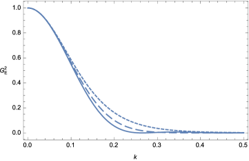
Figure 2: Gaussian (dashed), dipole (dotted) and uniformly charged sphere (solid) parameterizations of nuclear form factor $G_{E}^{2}(k^{2})$.

The momentum integration in (19) can be done analytically, so that the Zemach correction with the Gaussian and uniformly charged sphere parameterizations has the form (numerical results are presented in Tables 2-4 for these two parametrizations):

$$\Delta E^{hfs}_{str,G}=-E_{F}\frac{72}{\sqrt{3\pi}}\mu Z\alpha r_{N},~{}~{}~{}\Delta E^{hfs}_{str,U}=-E_{F}\frac{72\sqrt{5}}{35\sqrt{3}}\mu Z\alpha r_{N}.$$ (21)

Table 4: Hyperfine splittings of S-states in muonic ions $(\mu~{}^{10}_{5}B)^{4+}$ and $(\mu~{}^{11}_{5}B)^{4+}$.

No.	Contribution to the splitting	$(\mu~{}^{10}_{5}B)^{4+}$, meV		$(\mu~{}^{11}_{5}B)^{4+}$, meV
		1S	2S	1S	2S
1	Contribution of order $\alpha^{4}$,	11420.56	1427.57	19548.21	2443.53
	the Fermi energy
2	Muon AMM contribution	13.33	1.67	22.82	2.85
3	Relativistic correction	22.83	4.04	39.08	6.92
	of order $\alpha^{6}$
4	Nuclear structure correction	G; -1395.72	G: -174.46	G: -2370.05	G: -296.26
	of order $\alpha^{5}$	U: -1422.43	U: -177.80	U: -2415.42	U: -301.93
5	Nuclear structure and recoil	—	—	G: 36.68	G: 4.59
6	Nuclear structure correction	67.06	6.81	112.97	11.47
	of order $\alpha^{6}$ in $1\gamma$ interaction
7	Nuclear structure correction in second	-46.40	-15.69	-78.15	-26.45
	order perturbation theory
8	Vacuum polarization contribution	50.99	6.51	87.31	11.14
	of order $\alpha^{5}$ in first order PT
9	Vacuum polarization contribution	123.21	11.38	210.99	19.49
	of order $\alpha^{5}$ in second order PT
10	Muon vacuum polarization contribution	1.10	0.14	1.89	0.24
	of order $\alpha^{6}$ in first order PT
11	Muon vacuum polarization contribution	1.21	0.15	2.07	0.26
	of order $\alpha^{6}$ in second order PT
12	Vacuum polarization contribution	0.71	0.09	1.21	0.15
	of order $\alpha^{6}$ in first order PT
13	Vacuum polarization contribution	1.63	0.15	2.79	0.27
	of order $\alpha^{6}$ in second order PT
14	Nuclear structure and vacuum	-20.80	-2.60	-35.06	-4.38
	polarization correction of order $\alpha^{6}$
15	Nuclear structure and muon vacuum	-1.90	-0.24	-3.26	-0.41
	polarization correction of order $\alpha^{6}$
16	Hadron vacuum polarization	0.81	0.10	1.38	0.17
	contribution of order $\alpha^{6}$
17	Radiative nuclear finite size	-4.76	-0.59	-8.18	-1.02
	correction of order $\alpha^{6}$
	Summary contribution	10233.86	1265.03	17572.70	2172.56

Acting as in the case of the one-photon interaction, we can present the contribution of two-photon interactions to HFS at $F=2$ in the form:

$$\Delta E^{hfs}_{2\gamma}(F=2)=-\frac{(Z\alpha)^{2}}{640\pi^{2}m_{1}^{2}m_{2}^{2}}|\psi(0)|^{2}\int\frac{id^{4}k(k^{2}-2k_{0}m_{2})}{k^{4}(k^{4}-4k_{0}^{2}m_{1}^{2})(k^{4}-4k_{0}^{2}m_{2}^{2})}Tr\bigl{\{}(\hat{q}_{1}+m_{1})\times$$ (22)

$$[\gamma_{\mu}(\hat{p}_{1}-\hat{k}+m_{1})\gamma_{\nu}(k^{2}+2k_{0}m_{1})+\gamma_{\nu}(\hat{p}_{1}+\hat{k}+m_{1})\gamma_{\mu}(k^{2}-2k_{0}m_{1})](\hat{p}_{1}+m_{1})(1+\hat{v})\gamma_{\rho}(\hat{p}_{2}-m_{2})\times$$

$${\cal O}_{\alpha\nu\sigma}(k)(-\hat{p}_{2}-\hat{k}+m_{2})[g_{\sigma\tau}-\frac{1}{3}\gamma_{\sigma}\gamma_{\tau}-\frac{2}{3m_{2}^{2}}(p_{2}+k)_{\sigma}(p_{2}+k)_{\tau}+\frac{1}{3m_{2}}(\gamma_{\sigma}(p_{2}+k)_{\tau}-\gamma_{\tau}(p_{2}+k)_{\sigma})]\times$$

$${\cal O}_{\tau\mu\beta}(-k)(\hat{q}_{2}-m_{2})\gamma_{\lambda}(1+\hat{v})\bigr{\}}\hat{\Pi}_{\beta\alpha\lambda\rho},$$

where $k$ is a loop momentum, and $k_{0}$ its zero component. We also give for completeness analogous expressions for two states in (13) with $F=1,S=0$ and $F=1,S=1$:

$$\Delta E^{hfs}_{2\gamma}(F=1,S=0)=-\frac{(Z\alpha)^{2}}{384\pi^{2}m_{1}^{2}m_{2}^{2}}|\psi(0)|^{2}\int\frac{id^{4}k(k^{2}-2k_{0}m_{2})}{k^{4}(k^{4}-4k_{0}^{2}m_{1}^{2})(k^{4}-4k_{0}^{2}m_{2}^{2})}Tr\bigl{\{}(\hat{q}_{1}+m_{1})\times$$ (23)

$$[\gamma_{\mu}(\hat{p}_{1}-\hat{k}+m_{1})\gamma_{\nu}(k^{2}+2k_{0}m_{1})+\gamma_{\nu}(\hat{p}_{1}+\hat{k}+m_{1})\gamma_{\mu}(k^{2}-2k_{0}m_{1})](\hat{p}_{1}+m_{1})(1+\hat{v})\gamma_{5}(\hat{p}_{2}-m_{2})\times$$

$${\cal O}_{\alpha\nu\sigma}(k)(-\hat{p}_{2}-\hat{k}+m_{2})[g_{\sigma\tau}-\frac{1}{3}\gamma_{\sigma}\gamma_{\tau}-\frac{2}{3m_{2}^{2}}(p_{2}+k)_{\sigma}(p_{2}+k)_{\tau}+\frac{1}{3m_{2}}(\gamma_{\sigma}(p_{2}+k)_{\tau}-\gamma_{\tau}(p_{2}+k)_{\sigma})]\times$$

$${\cal O}_{\tau\mu\beta}(-k)(\hat{q}_{2}-m_{2})\gamma_{5}(1+\hat{v})\bigr{\}}(-g_{\alpha\beta}+v_{\alpha}v_{\beta}),$$

$$\Delta E^{hfs}_{2\gamma}(F=1,S=1)=-\frac{(Z\alpha)^{2}}{768\pi^{2}m_{1}^{2}m_{2}^{2}}|\psi(0)|^{2}\int\frac{id^{4}k(k^{2}-2k_{0}m_{2})}{k^{4}(k^{4}-4k_{0}^{2}m_{1}^{2})(k^{4}-4k_{0}^{2}m_{2}^{2})}Tr\bigl{\{}(\hat{q}_{1}+m_{1})\times$$ (24)

$$[\gamma_{\mu}(\hat{p}_{1}-\hat{k}+m_{1})\gamma_{\nu}(k^{2}+2k_{0}m_{1})+\gamma_{\nu}(\hat{p}_{1}+\hat{k}+m_{1})\gamma_{\mu}(k^{2}-2k_{0}m_{1})](\hat{p}_{1}+m_{1})(1+\hat{v})\gamma_{\sigma_{1}}\varepsilon_{\alpha\sigma_{1}\rho_{1}\omega_{1}}v_{\rho_{1}}\times$$

$$(\hat{p}_{2}-m_{2}){\cal O}_{\alpha\nu\sigma}(k)(-\hat{p}_{2}-\hat{k}+m_{2})[g_{\sigma\tau}-\frac{1}{3}\gamma_{\sigma}\gamma_{\tau}-\frac{2}{3m_{2}^{2}}(p_{2}+k)_{\sigma}(p_{2}+k)_{\tau}+\frac{1}{3m_{2}}(\gamma_{\sigma}(p_{2}+k)_{\tau}-$$

$$\gamma_{\tau}(p_{2}+k)_{\sigma})]{\cal O}_{\tau\mu\beta}(-k)(\hat{q}_{2}-m_{2})\gamma_{\epsilon_{1}}(1+\hat{v})\varepsilon_{\beta\epsilon_{1}\tau_{1}\lambda_{1}}v_{\tau_{1}}\bigr{\}}(-g_{\lambda_{1}\omega_{1}}+v_{\lambda_{1}}v_{\omega_{1}}).$$

There is also an off-diagonal matrix element between states with $F=1,S=0$ and $F=1,S=1$, which we omit here. The expressions (21) - (24) are presented in a form convenient for the subsequent calculation in the package Form form . As a result the value of the hyperfine splitting is determined in Euclidean space by the following formula:

$$\Delta E^{hfs}(nS)=|\psi_{nS}(0)|^{2}\int d^{4}kV_{2\gamma}(k)=\frac{64}{9}\frac{(Z\alpha)^{2}}{\pi^{2}}|\psi_{nS}(0)|^{2}\int\frac{d^{4}k}{k^{4}(k^{4}+4m_{1}^{2}k_{0}^{2})(k^{4}+4m_{2}^{2}k_{0}^{2})}\times$$ (25)

$$\Bigl{[}F_{1}F_{2}\Bigl{(}k^{6}-k^{4}k_{0}^{2}+\frac{4}{15}\frac{k^{4}k_{0}^{4}}{m_{2}^{2}}-\frac{7}{10}\frac{k^{6}k_{0}^{2}}{m_{2}^{2}}+\frac{13}{30}\frac{k^{8}}{m_{2}^{2}}\Bigr{)}+F_{2}F_{4}\Bigl{(}-\frac{1}{30}\frac{k^{2}k_{0}^{6}}{m_{2}^{2}}+\frac{1}{15}\frac{k^{4}k_{0}^{4}}{m_{2}^{2}}-\frac{1}{30}\frac{k^{6}k_{0}^{2}}{m_{2}^{2}}\Bigr{)}+$$

$$F_{2}F_{3}\Bigl{(}-\frac{1}{15}\frac{k^{2}k_{0}^{6}}{m_{2}^{2}}+\frac{11}{60}\frac{k^{4}k_{0}^{4}}{m_{2}^{2}}-\frac{7}{60}\frac{k^{8}}{m_{2}^{2}}\Bigr{)}+F_{1}F_{4}\Bigl{(}-\frac{1}{5}\frac{k^{2}k_{0}^{6}}{m_{2}^{2}}+\frac{3}{10}\frac{k^{4}k_{0}^{4}}{m_{2}^{2}}-\frac{1}{10}\frac{k^{8}}{m_{2}^{2}}\Bigr{)}+$$

$$F_{2}^{2}\Bigl{(}\frac{1}{15}\frac{k^{2}k_{0}^{6}}{m_{2}^{2}}-\frac{1}{6}k^{2}k_{0}^{4}-\frac{2}{15}\frac{k^{4}k_{0}^{4}}{m_{2}^{2}}+\frac{1}{6}k^{4}k_{0}^{2}+\frac{23}{120}\frac{k^{6}k_{0}^{2}}{m_{2}^{2}}-\frac{1}{4}\frac{k^{8}}{m_{2}^{2}}\Bigr{)}\Bigr{]}.$$

When investigating this expression, it is useful to distinguish the Zemach correction, which is determined by the integral

$$J=\int_{0}^{\infty}\int_{0}^{\pi}\frac{k\sin^{2}\phi dkd\phi F_{1}(k^{2})F_{2}(k^{2})}{(k^{2}+4m_{1}^{2}\cos^{2}\phi)(k^{2}+4m_{2}^{2}\cos^{2}\phi)}=\frac{\pi}{2(m_{1}+m_{2})}\int_{0}^{\infty}\frac{dk}{k^{2}}F_{1}(k^{2})F_{2}(k^{2})+$$ (26)

$$\frac{\pi}{4(m_{1}^{2}-m_{2}^{2})}\int_{0}^{\infty}\frac{dk}{k^{2}}[\sqrt{k^{2}+4m_{1}^{2}}-2m_{1}-\sqrt{k^{2}+4m_{2}^{2}}+2m_{2}]F_{1}(k^{2})F_{2}(k^{2}).$$

The divergence in the first term on the right-hand side of (26) is compensated by the subtraction term

$$\Delta E^{hfs}_{iter}=\frac{64}{9}\frac{(Z\alpha)^{2}}{\pi^{2}}|\psi(0)|^{2}\int_{0}^{\infty}\frac{2\pi^{2}F_{2}(0)}{(m_{1}+m_{2})k^{2}}dk.$$ (27)

Thus, we have in (25) the main contribution (the Zemach correction) and the recoil correction $m_{1}/m_{2}$. In the case of Li nucleus with spin 1 the expression similar to (25) was obtained in apm3 for muonic deuterium. We use it for corresponding numerical estimates of nuclear structure and recoil corrections in ${}^{6}_{3}Li$. The recoil effects for the nucleus ${}^{10}_{5}B$ with spin 3 are neglected.

The form factors $F_{i}(k^{2})$ are expressed in terms of $G_{E0}$, $G_{E2}$, $G_{M1}$, $G_{M3}$ for which the Gaussian parametrization is used in numerical calculations of integrals with respect to k. The values of the form factors at zero have the form:

$$G_{E0}(0)=1,~{}~{}~{}G_{M1}(0)=\frac{m_{2}\mu_{N}}{m_{p}Z},~{}~{}~{}G_{E2}(0)=m_{2}^{2}Q,~{}~{}~{}G_{M3}(0)=\frac{m_{2}}{m_{p}Z}m_{2}^{2}\Omega.$$ (28)

Different parameters of light nucleus (Li, Be, B) were investigated in electron scattering experiments scat ; fuller . The nucleus multiple moments are presented in Table 1. Some of them are unknown with good accuracy, but, nevertheless, one can obtain approximate estimates of the corresponding contributions. After angular analytical integration in (25) we make numerical integration over $k$. Obtained results for nuclear structure and recoil corrections are presented in Tables 2-4 in separate lines.

Figure 3: Nuclear structure effects in one-photon interaction (c) and in second order perturbation theory (d). $\tilde{G}$ is the reduced Coulomb Green’s function.

Another correction for the structure of the nucleus of order $\alpha^{6}$, which must be discussed, is obtained as a result of the decomposition of the magnetic form factor of the nucleus see Fig. 3(a)). The contribution to the interaction potential and HFS in this case has the form apm2008 ; apm2 :

$$\Delta V^{hfs}_{1\gamma,str}(r)=\frac{4\pi\alpha\mu_{N}}{9m_{1}m_{p}}r_{M}^{2}({\bf s}_{1}{\bf s}_{2})\nabla^{2}\delta({\bf r}),$$ (29)

$$\Delta E^{hfs}_{1\gamma,str}=\frac{2}{3}\mu^{2}Z^{2}\alpha^{2}r_{M}^{2}\frac{3n^{2}+1}{n^{2}}E_{F}(nS).$$ (30)

Numerical values on the basis (30) can be obtained assuming that $r_{M}^{2}=r_{E}^{2}$. They are in line 11 of Tables 2-4.

In second order PT we should take into account a term in which the potential

$$\Delta V^{C}_{str,1\gamma}(k)=-\frac{Z\alpha}{{\bf k}^{2}}\left[\frac{3}{(kR)^{3}}\left(\sin kR-kR\cos kR\right)-1\right]$$ (31)

is considered as a perturbation. The Fourier transform of (31) is

$$\Delta V^{C}_{str,1\gamma}(r)=-\frac{Z\alpha}{4R^{3}r}(r-R)(r+2R)(R-r+|r-R|).$$ (32)

Using the Green’s functions (43) and (44) (see section III) we perform the analytical integration in second order PT. It gives the following result:

$$\Delta E^{hfs}_{str,sopt}(1S)=-E_{F}(1S)\frac{R^{2}W^{2}}{4}\bigl{[}-\frac{4}{75}(-53+15C+15\ln RW+\frac{RW}{12}\bigl{(}-15+4C+4\ln RW\bigr{)}\bigl{]},$$ (33)

$$\Delta E^{hfs}_{str,sopt}(2S)=E_{F}(2S)\frac{R^{2}W^{2}}{4}\bigl{[}\frac{4}{75}(-107+60C+60\ln RW)+\frac{RW}{3}(17-8C-8\ln RW)\bigr{]},$$ (34)

where we present an expansions in $(RW)$ up to terms of first order in square brackets ($RW(^{6}_{3}Li)=0.038$, $RW(^{7}_{3}Li)=0.036$, $RW(^{9}_{4}Be)=0.050$, $RW(^{10}_{5}B)=0.060$, $RW(^{11}_{5}B)=0.060$). Numerical values of (33) and (34) are sufficiently important (see line 7 of Tables 2-4).

Figure 4: Effects of one- and two-loop vacuum polarization in one-photon interaction.

III Effects of one- and two-loop vacuum polarization in first and second orders of perturbation theory

Another our task is to analyse different vacuum polarization corrections to the total value of the hyperfine splitting. Primarily, we have to calculate a contribution of one-loop vacuum polarization contribution in first order PT. Corresponding potential can be obtained in momentum representation after a standard modification of hyperfine muon-nucleus interaction due to vacuum polarization effect borie1 ; borie2 ; kp1996 ; sgk1 ; sgk2 ; t4 . In coordinate representation it is defined by the following integral expression:

$$\Delta V^{hfs}_{1\gamma,vp}(r)=\frac{4\alpha g_{N}(1+a_{\mu})}{3m_{1}m_{p}}({\bf s}_{1}{\bf s}_{2})\frac{\alpha}{3\pi}\int_{1}^{\infty}\rho(\xi)d\xi\left(\pi\delta({\bf r})-\frac{m_{e}^{2}\xi^{2}}{r}e^{-2m_{e}\xi r}\right),$$ (35)

where $g_{N}=\mu_{N}/s_{2}$, spectral function $\rho(\xi)=\sqrt{\xi^{2}-1}(2\xi^{2}+1)/\xi^{4}$. We include in (35) the anomalous magnetic moment of muon, which leads to the additional contribution of order $\alpha^{6}$. Averaging (35) over wave functions (4) and (5), we get the contribution of order $\alpha^{5}$ to hyperfine structure of $1S-$ and $2S$-states ($a_{1}=m_{e}/W$, $W=\mu Z\alpha$):

$$\Delta E_{1\gamma,vp}^{hfs}(1S)=\frac{4\alpha^{2}(Z\alpha)^{3}\mu^{3}g_{N}(1+a_{\mu})}{9m_{1}m_{p}\pi}<({\bf s}_{1}{\bf s}_{2})>\int_{1}^{\infty}\rho(\xi)d\xi\left[1-\frac{m_{e}^{2}\xi^{2}}{W^{2}}\int_{0}^{\infty}xdxe^{-x\left(1+\frac{m_{e}\xi}{W}\right)}\right]=$$ (36)

$$E_{F}(1S)\frac{\alpha(1+a_{\mu})}{9\pi\sqrt{1-a_{1}^{2}}}\Bigl{[}\sqrt{1-a_{1}^{2}}(1+6a_{1}^{2}-3\pi a_{1}^{3})+(6-3a_{1}^{2}+5a_{1}^{4})\ln\frac{1+\sqrt{1-a_{1}^{2}}}{a_{1}}\Bigr{]},$$

$$\Delta E_{1\gamma,vp}^{hfs}(2S)=\frac{\alpha^{2}(Z\alpha)^{3}\mu^{3}g_{N}(1+a_{\mu})}{18m_{1}m_{p}\pi}<({\bf s}_{1}{\bf s}_{2})>\int_{1}^{\infty}\rho(\xi)d\xi\times$$ (37)

$$\left[1-\frac{4m_{e}^{2}\xi^{2}}{W^{2}}\int_{0}^{\infty}x\left(1-\frac{x}{2}\right)^{2}dxe^{-x\left(1+\frac{2m_{e}\xi}{W}\right)}\right]=$$

$$E_{F}(2S)\frac{\alpha(1+a_{\mu})}{18\pi(4a_{1}^{2}-1)^{5/2}}\Bigl{\{}\sqrt{4a_{1}^{2}-1}[11+2a_{1}^{2}(-29+8a_{1}(-22a_{1}+48a_{1}3-3\pi(4a_{1}^{2}-1)^{2}))]+$$

$$12(1-10a_{1}^{2}+66a_{1}^{4}-160a_{1}^{6}+256a_{1}^{8})\arctan\sqrt{4a_{1}^{2}-1}\Bigr{\}}.$$

We present in detail the results of (36)-(37) to demonstrate the general structure of the obtained analytical expressions. After integrating over particle coordinates, the results have a fairly simple form, but the following integration over the spectral parameters gives, as a rule, rather cumbersome expressions, which we will omit in the following.

With a simple replacement $m_{e}$ to muon mass $m_{1}$ in equations (36) and (37) one can obtain the muon vacuum polarization correction to HFS of order $\alpha^{6}$. The numerical values of the muon vacuum polarization corrections are included in Table 2-4 in the corresponding line (line 6). Another contribution of order $\alpha^{6}$ is represented by two-loop vacuum polarization diagrams (see Fig. 4(b,c,d) (the Källen and Sabry potential sabry ). The construction of the interaction potentials from these diagrams is completely analogous to (35). They have the form of a double and a single spectral integral in coordinate space apm2004 ; apm2008 :

$$\Delta V_{1\gamma,vp-vp}^{hfs}(r)=\frac{4\pi\alpha g_{N}(1+a_{\mu})}{3m_{1}m_{p}}({\bf s}_{1}{\bf s}_{2})\left(\frac{\alpha}{3\pi}\right)^{2}\int_{1}^{\infty}\rho(\xi)d\xi\int_{1}^{\infty}\rho(\eta)d\eta\times$$ (38)

$$\times\left[\delta({\bf r})-\frac{m_{e}^{2}}{\pi r(\eta^{2}-\xi^{2})}\left(\eta^{4}e^{-2m_{e}\eta r}-\xi^{4}e^{-2m_{e}\xi r}\right)\right],$$

$$\Delta V_{1\gamma,2-loop~{}vp}^{hfs}(r)=\frac{8\alpha^{3}g_{N}(1+a_{\mu})}{9\pi^{2}m_{1}m_{p}}({\bf s}_{1}{\bf s}_{2})\int_{0}^{1}\frac{f(v)dv}{1-v^{2}}\left[\pi\delta({\bf r})-\frac{m_{e}^{2}}{r(1-v^{2})}e^{-\frac{2m_{e}r}{\sqrt{1-v^{2}}}}\right],$$ (39)

where two-loop spectral function

$$f(v)=v\Bigl{\{}(3-v^{2})(1+v^{2})\left[Li_{2}\left(-\frac{1-v}{1+v}\right)+2Li_{2}\left(\frac{1-v}{1+v}\right)+\frac{3}{2}\ln\frac{1+v}{1-v}\ln\frac{1+v}{2}-\ln\frac{1+v}{1-v}\ln v\right]$$ (40)

$$+\left[\frac{11}{16}(3-v^{2})(1+v^{2})+\frac{v^{4}}{4}\right]\ln\frac{1+v}{1-v}+\left[\frac{3}{2}v(3-v^{2})\ln\frac{1-v^{2}}{4}-2v(3-v^{2})\ln v\right]+\frac{3}{8}v(5-3v^{2})\Bigr{\}},$$

where $Li_{2}(z)$ is the Euler dilogarithm. Averaging (38)-(39) over wave functions (5)-(6) the integration over $r$ can be done analytically, while two other integrations over $\xi$ and $\eta$ are calculated numerically with the use of Wolfram Mathematica. Summary two-loop vacuum polarization correction of order $\alpha^{6}$ is written in Tables 2-4 (line 7).

To achieve the desired accuracy of calculations one-loop and two-loop contributions of order $\alpha^{5}$ and $\alpha^{6}$ to HFS have to be taken into account in second order perturbation theory. The second order perturbation theory (PT) corrections to the energy spectrum are determined by the reduced Coulomb Green’s function $\tilde{G}_{n}({\bf r},{\bf r^{\prime}})$ The radial part $\tilde{g}_{nl}(r,r^{\prime})$ of $\tilde{G}_{n}({\bf r},{\bf r^{\prime}})$ was obtained in hameka in the form of the Sturm expansion in the Laguerre polynomials. The main contribution of the electron vacuum polarization to HFS in second order PT (sopt) has the form (see Fig. 5(a)):

$$\Delta E^{hfs}_{sopt~{}vp~{}1}=2<\psi|\Delta V^{C}_{VP}\cdot\tilde{G}\cdot\Delta V_{B}^{hfs}|\psi>,$$ (41)

where the Coulomb potential, modified by the one-loop vacuum polarization effect, has the form

$$\Delta V^{C}_{vp}(r)=\frac{\alpha}{3\pi}\int_{1}^{\infty}\rho(\xi)d\xi\left(-\frac{Z\alpha}{r}\right)e^{-2m_{e}\xi r}.$$ (42)

Figure 5: Effects of one- and two-loop vacuum polarization in second order PT.

Since hyperfine part of the Breit potential $\Delta V_{B}^{hfs}(r)$ is proportional to $\delta({\bf r})$, it is necessary to use the reduced Coulomb Green’s function with one zero argument. For this case it was obtained on the basis of the Hostler representation after a subtraction of the pole term in hameka . We represent for the sake of completeness the explicit expressions for the Green’s functions, used in later calculations:

$$\tilde{G}_{1S}({\bf r},0)=\frac{Z\alpha\mu^{2}}{4\pi}\frac{e^{-x}}{x}g_{1S}(x),~{}~{}~{}g_{1S}(x)=\left[4x(\ln 2x+C)+4x^{2}-10x-2\right],$$ (43)

$$\tilde{G}_{2S}({\bf r},0)=-\frac{Z\alpha\mu^{2}}{4\pi}\frac{e^{-x/2}}{2x}g_{2S}(x),~{}~{}~{}g_{2S}(x)=\left[4x(x-2)(\ln x+C)+x^{3}-13x^{2}+6x+4\right],$$ (44)

where $C=0.5772...$ is the Euler constant and $x=Wr$. Then the necessary vacuum polarization corrections of order $\alpha^{5}$ to HFS of muonic ions can be presented as follows:

$$\Delta E^{hfs}_{sopt~{}vp~{}1}(1S)=-E_{F}(1S)\frac{2\alpha}{3\pi}(1+a_{\mu})\int_{1}^{\infty}\rho(\xi)d\xi\int_{0}^{\infty}e^{-2x\left(1+\frac{m_{e}\xi}{W}\right)}g_{1S}(x)dx,$$ (45)

$$\Delta E^{hfs}_{sopt~{}vp~{}1}(2S)=E_{F}(2S)\frac{\alpha}{3\pi}(1+a_{\mu})\int_{1}^{\infty}\rho(\xi)d\xi\int_{0}^{\infty}e^{-x\left(1+\frac{2m_{e}\xi}{W}\right)}g_{2S}(x)(1-\frac{x}{2})dx,$$ (46)

where we use its designation by the index $(sopt~{}vp~{}1)$. The result of integration is in line 5 of Tables 2-4. The factor $(1+a_{\mu})$ is included in (45) and (46), therefore these expressions contain corrections of orders $\alpha^{5}$ and $\alpha^{6}$. Changing $m_{e}\to m_{1}$ in (45)-(46) we calculate one-loop muon vacuum polarization contribution in second order PT of order $\alpha^{6}$ (see line 7 of Tables 2-4).

Two-loop corrections in Fig. 5(b,c,d,e) are of order $\alpha^{6}$. Let us consider first contribution which is related with potentials (35) and (42), reduced Coulomb Green’s functions (43), (44) and reduced Coulomb Green’s function with nonzero arguments. General structure of this contribution takes the form:

$$\Delta E^{hfs}_{sopt~{}vp~{}2}=2<\psi|\Delta V^{hfs}_{1\gamma,vp}\cdot\tilde{G}\cdot\Delta V^{C}_{vp}|\psi>.$$ (47)

The convenient representation for reduced Coulomb Green’s function with nonzero arguments was obtained in hameka :

$$\tilde{G}_{1S}(r,r^{\prime})=-\frac{Z\alpha\mu^{2}}{\pi}e^{-(x_{1}+x_{2})}g_{1S}(x_{1},x_{2}),$$ (48)

$$g_{1S}(x_{1},x_{2})=\frac{1}{2x_{>}}-\ln 2x_{>}-\ln 2x_{<}+Ei(2x_{<})+\frac{7}{2}-2C-(x_{1}+x_{2})+\frac{1-e^{2x_{<}}}{2x_{<}},$$

$$\tilde{G}_{2S}(r,r^{\prime})=-\frac{Z\alpha\mu^{2}}{16\pi x_{1}x_{2}}e^{-\frac{x_{1}+x_{2}}{2}}g_{2S}(x_{1},x_{2}),$$ (49)

$$g_{2S}(x_{1},x_{2})=8x_{<}-4x^{2}_{<}+8x_{>}+12x_{<}x_{>}-26x^{2}_{<}x_{>}+2x^{3}_{<}x_{>}-4x^{2}_{>}-26x_{<}x^{2}_{>}+23x^{2}_{<}x^{2}_{>}-$$

$$-x^{3}_{<}x^{2}_{>}+2x_{<}x^{3}_{>}-x^{2}_{<}x^{3}_{>}+4e^{x_{<}}(1-x_{<})(x_{>}-2)x_{>}+4(x_{<}-2)x_{<}(x_{>}-2)x_{>}\times$$

$$\times[-2C+Ei(x_{<})-\ln(x_{<})-\ln(x_{>})],$$

where $x_{1}=Wr$, $x_{2}=Wr^{\prime}$, $x_{<}=min(x_{1},x_{2})$, $x_{>}=max(x_{1},x_{2})$, $C=0.577216...$ is the Euler constant, and $Ei(x)$ is the integral exponential function. The substitution of (35), (42), (43), (44), (48) and (49) into (47) provides two terms for each $1S$ and $2S$ level in integral form:

$$\Delta E^{hfs}_{sopt~{}vp~{}21}(1S)=-2E_{F}(1S)\frac{\alpha^{2}}{9\pi^{2}}(1+a_{\mu})\int_{1}^{\infty}\rho(\xi)d\xi\int_{1}^{\infty}\rho(\eta)d\eta\int_{0}^{\infty}dxe^{-2x\left(1+\frac{m_{e}\eta}{W}\right)}g_{1S}(x),$$ (50)

$$\Delta E^{hfs}_{sopt~{}vp~{}22}(1S)=2E_{F}(1S)\frac{\alpha^{2}}{9\pi^{2}}(1+a_{\mu})\frac{16m_{e}^{2}}{W^{2}}\int_{1}^{\infty}\rho(\xi)\xi^{2}d\xi\times$$ (51)

$$\times\int_{1}^{\infty}\rho(\eta)d\eta\int_{0}^{\infty}x_{1}dx_{1}e^{-2x_{1}\left(1+\frac{m_{e}\eta}{W}\right)}\int_{0}^{\infty}x_{2}dx_{2}e^{-2x_{2}\left(1+\frac{m_{e}\xi}{W}\right)}g_{1S}(x_{1},x_{2}),$$

$$\Delta E^{hfs}_{sopt~{}vp~{}21}(2S)=E_{F}(2S)\frac{\alpha^{2}}{9\pi^{2}}(1+a_{\mu})\int_{1}^{\infty}\rho(\xi)d\xi\int_{1}^{\infty}\rho(\eta)d\eta\int_{0}^{\infty}\left(1-\frac{x}{2}\right)dxe^{-x\left(1+\frac{2m_{e}\eta}{W}\right)}g_{2S}(x),$$ (52)

$$\Delta E^{hfs}_{sopt~{}vp~{}22}(2S)=-E_{F}(2S)\frac{\alpha^{2}}{9\pi^{2}}(1+a_{\mu})\frac{2m_{e}^{2}}{W^{2}}\int_{1}^{\infty}\rho(\xi)\xi^{2}d\xi\times$$ (53)

$$\times\int_{1}^{\infty}\rho(\eta)d\eta\int_{0}^{\infty}\left(1-\frac{x_{1}}{2}\right)dx_{1}e^{-x_{1}\left(1+\frac{2m_{e}\xi}{W}\right)}\int_{0}^{\infty}\left(1-\frac{x_{2}}{2}\right)dx_{2}e^{-x_{2}\left(1+\frac{2m_{e}\eta}{W}\right)}g_{2S}(x_{1},x_{2}).$$

Separately, the contributions (27), (28) and (35),(36) are divergent but their sum is finite. Corresponding numerical values are:

$$\Delta E^{hfs}_{vp,vp}(1S)=\begin{cases}{}_{3}^{6}Li:0.05~{}meV\\ {}_{3}^{7}Li:0.20~{}meV\\ {}_{4}^{9}Be:-0.21~{}meV;\\ {}_{5}^{10}B:0.65~{}meV\\ {}_{5}^{11}B:1.11~{}meV\end{cases}\Delta E^{hfs}_{vp,vp}(2S)=\begin{cases}{}_{3}^{6}Li:0.01~{}meV\\ {}_{3}^{7}Li:0.02~{}meV\\ {}_{4}^{9}Be:-0.02~{}meV.\\ {}_{5}^{10}B:0.06~{}meV\\ {}_{5}^{11}B:0.11~{}meV\end{cases}$$ (54)

The contributions of two other amplitudes in Fig. 5(c,d,e) to HFS can be calculated by means of (47), where the replacement of the potential (42) on the following potentials should be made apm2008 :

$$\Delta V^{C}_{VP-VP}(r)=\left(\frac{\alpha}{3\pi}\right)^{2}\int_{1}^{\infty}\rho(\xi)d\xi\int_{1}^{\infty}\rho(\eta)d\eta\left(-\frac{Z\alpha}{r}\right)\frac{1}{\xi^{2}-\eta^{2}}\left(\xi^{2}e^{-2m_{e}\xi r}-\eta^{2}e^{-2m_{e}\eta r}\right),$$ (55)

$$\Delta V^{C}_{2-loop~{}VP}(r)=-\frac{2Z\alpha^{3}}{3\pi^{2}r}\int_{0}^{1}\frac{f(v)dv}{(1-v^{2})}e^{-\frac{2m_{e}r}{\sqrt{1-v^{2}}}}.$$ (56)

Omitting further intermediate expressions we include in Tables 2-4 total numerical values of two-loop vacuum polarization corrections in second order PT (Fig. 5(b,c,d,e)) in line 9.

There is another correction for the polarization of the vacuum, which also includes the effect of the nuclear structure discussed in Section II (see Fig. 6). To calculate it, it is necessary to use the potential $V_{2\gamma}(k)$ from (25), modifying it accordingly. As a result, the contribution to the HFS spectrum is determined by the following expression (the factor 2 corresponds to two exchange photons):

$$E_{2\gamma,vp}^{hfs}=-\frac{2\mu^{3}Z^{3}\alpha^{4}}{9\pi^{2}n^{3}}\int\frac{V_{2\gamma}(k)d^{4}k}{k^{3}}\bigl{[}5k^{3}-12m_{e}k^{2}-6(k^{2}-2m_{e}^{2})\sqrt{k^{2}+4m_{e}^{2}}Arcth[\frac{k}{\sqrt{k^{2}+4m_{e}^{2}}}\bigr{]}.$$ (57)

Numerical integration in (39) can be carried out exactly as in (25) (line 12 of Tables 2-4). The contribution of muon VP in $2\gamma$-amplitudes with the nuclear structure is written in line 13 of Tables 2-4.

Figure 6: Two photon exchange amplitudes accounting for effects of vacuum polarization and nuclear structure. The wavy line denotes the photon. The bold point denotes the nucleus vertex function.

In order to increase the accuracy of the calculation we consider also hadron vacuum polarization (HVP) contribution which arises, like the electron polarization of the vacuum, in the first order PT, in the second order PT, and in two-photon exchange amplitudes. To obtain it we use a standard replacement in photon propagator of the form faustov1999 .

$$\frac{1}{k^{2}}\to\left(\frac{\alpha}{\pi}\right)\int_{s_{th}}^{\infty}\frac{\rho_{had}(s)ds}{k^{2}+s},~{}~{}~{}\rho_{had}(s)=\frac{(s-4m_{\pi}^{2})^{3/2}}{12s^{5/2}}|F_{\pi}(s)|^{2},$$ (58)

where $F_{\pi}(s)$ is the pion form factor. Total hadron vacuum polarization contribution is presented in Tables 2-4 (line 14).

IV Radiative corrections to two photon exchange diagrams.

The results already obtained in the Tables 2-4 clearly show that the corrections to the structure of the nucleus are dominant. In this connection, it seems useful to consider another correction for the structure of the nucleus of order $\alpha^{6}$ shown in Fig. 7 to refine the results. The amplitudes of two-photon exchange with radiative corrections to the muon line can be calculated in the framework of the calculation method formulated in Section II. For a radiative photon, the Fried-Yennie gauge is used, in which each of the amplitudes in Fig. 7 (muon self-energy, muon vertex correction, amplitude with the spanning photon) can be represented by a finite integral expression. The general structure of the amplitudes in Fig. 7 is the following:

$${i\cal M}=\frac{(Z\alpha)^{2}}{\pi^{2}}\int d^{4}k\left[\bar{u}(q_{1})L_{\mu\nu}u(p_{1})\right]D_{\mu\omega}(k)D_{\nu\lambda}(k)\left[\bar{v}_{\rho}(p_{2}){\cal O}_{\rho\omega\beta}{\cal D}_{\beta\tau}(p_{2}+k){\cal O}_{\tau\lambda\alpha}v_{\alpha}(q_{2})\right],$$ (59)

where the vertex operator ${\cal O}_{\rho\omega\beta}$ describing the photon-nucleus interaction is determined by the nucleus electromagnetic form factors as in (8) for the nucleus of spin $3/2$.

The spin $3/2$ particle propagator and the photon propagator in the Coulomb gauge are equal to

$${\cal D}_{\alpha\beta}(p)=\frac{\hat{p}+m_{2}}{p^{2}-m_{2}^{2}+i0}\left[g_{\rho\beta}-\frac{1}{3}\gamma_{\rho}\gamma_{\beta}-\frac{2p_{\rho}p_{\beta}}{3m_{2}^{2}}-\frac{\gamma_{\rho}p_{\beta}-\gamma_{\beta}p_{\rho}}{3m_{2}}\right],$$ (60)

$$D_{\lambda\sigma}(k)=\frac{1}{k^{2}+i0}\left[g_{\lambda\sigma}+\frac{k_{\lambda}k_{\sigma}-k_{0}k_{\lambda}g_{\sigma 0}-k_{0}k_{\sigma}g_{\lambda 0}}{{\bf k}^{2}}\right].$$ (61)

The lepton tensor $L_{\mu\nu}$ is equal to a sum of three terms coming from three amplitudes in Fig. 7:

$$L_{\mu\nu}=L_{\mu\nu}^{se}+L_{\mu\nu}^{vertex}+L_{\mu\nu}^{jellyfish}.$$ (62)

All three terms of the lepton tensor were obtained in integral form and are written explicitly in apm2 ; eides1 ; eides2 ; eides3 .

Figure 7: Direct two-photon exchange amplitudes with radiative corrections to muon line giving contributions of order $E_{F}\alpha(Z\alpha)$ to the hyperfine structure. Wave line on the diagram denotes the photon. Bold point on the diagram denotes the vertex operator of the nucleus.

The construction of hyperfine potential by means of amplitudes in Fig. 7 in the case of the spin 3/2 nucleus can be performed by the method of projection operators as in section II. Neglecting the recoil effects in the denominator of the nucleus propagator we obtain that a sum of direct and crossed amplitudes is proportional to $\delta(k_{0})$:

$$\frac{1}{2m_{2}k_{0}+i0}+\frac{1}{-2m_{2}k_{0}+i0}=-\frac{i\pi}{m_{2}}\delta(k_{0}).$$ (63)

As a result three types of contributions of order $E_{F}\alpha(Z\alpha)$ to HFS of muonic ions of lithium, beryllium and boron are expressed in integral form over the loop momentum $k$ and the Feynman parameters:

$$\Delta E^{hfs}_{se}=E_{F}6\frac{\alpha(Z\alpha)}{\pi^{2}}\int_{0}^{1}xdx\int_{0}^{\infty}\frac{G_{E}(k^{2})G_{M}(k^{2})dk}{x+(1-x)k^{2}},$$ (64)

$$\Delta E^{hfs}_{vertex-1}=-E_{F}24\frac{\alpha(Z\alpha)}{\pi^{2}}\int_{0}^{1}dz\int_{0}^{1}xdx\int_{0}^{\infty}\frac{G_{E}(k^{2})G_{M}(k^{2})\ln[\frac{x+k^{2}z(1-xz)}{x}]dk}{k^{2}},$$ (65)

$$\Delta E^{hfs}_{vertex-2}=E_{F}8\frac{\alpha(Z\alpha)}{\pi^{2}}\int_{0}^{1}dz\int_{0}^{1}dx\int_{0}^{\infty}\frac{dk}{k^{2}}\biggl{\{}\frac{G_{E}(k^{2})G_{M}(k^{2})}{[x+k^{2}z(1-xz)]^{2}}\bigl{[}-2xz^{2}(1-xz)^{2}k^{4}+$$ (66)

$$zk^{2}(3x^{3}z-x^{2}(9z+1)+x(4z+7)-4)+x^{2}(5-x)\bigr{]}-\frac{1}{2}\biggr{\}},$$

$$\Delta E^{hfs}_{jellyfish}=E_{F}4\frac{\alpha(Z\alpha)}{\pi^{2}}\int_{0}^{1}(1-z)dz\int_{0}^{1}(1-x)dx\int_{0}^{\infty}\frac{G_{E}(k^{2})G_{M}(k^{2})dk}{[x+(1-xz)k^{2}]^{3}}$$ (67)

$$\times\bigl{[}6x+6x^{2}-6x^{2}z+2x^{3}-12x^{3}z-12x^{4}z+k^{2}(-6z+18xz+4xz^{2}+7x^{2}z-30x^{2}z^{2}-$$

$$2x^{2}z^{3}-36x^{3}z^{2}+12x^{3}z^{3}+24x^{4}z^{3})+k^{4}(9xz^{2}-31x^{2}z^{3}+34x^{3}z^{4}-12x^{4}z^{5}\bigr{]}$$

All contributions (64)-(67) are expressed in terms of electric and dipole magnetic form factors. The term $1/2$ in figure brackets (66) is related to the subtraction term of the quasipotential. All corrections (64), (65), (66), (67) are expressed through the convergent integrals. Numerical results for the corrections (64)-(67) are presented in Tables 2-4 (line 17).

V Conclusion

In this work we carry out a calculation of S-states hyperfine splittings in a number of muonic ions. We consider that light muonic ions of the lithium, beryllium and boron can be used in experiments of the CREMA collaboration. Our precise calculation of the HFS includes taking into account the various corrections of the fifth and sixth orders in $\alpha$, which were previously taken into account also in the study of the hyperfine structure of the spectrum of other muonic atoms apm1 ; apm2 ; apm3 ; apm4 . One significant difference between these calculations and the previous ones is due to the fact that in this paper we investigate the nuclei of spin 1, 3/2, 3. For spin 3/2 nuclei we have included the effects of two-photon interactions in the framework of quantum electrodynamics of spin particles 3/2. Corrections to the structure of the nucleus, which are determined by two-photon exchange amplitudes, as follows from the results of the Tables 2-4, play a very important role in achieving high accuracy of calculation. They are defined in our approach by the electromagnetic form factors of the nuclei, which in this case must be taken from experimental data. Intensive experimental studies of the scattering of leptons by light nuclei were carried out several dozen years ago. The results obtained then are reflected in scat ; fuller . We use these results, although the accuracy of determining all the required form factors is not very high, as would be desirable. For this reason, we use different parameterizations (Gaussian, uniformly charged sphere) for form factors and compared the numerical results for them to understand how they can differ. Complete numerical values for hyperfine splittings of S-levels are presented in the Tables 2-4 for the Gaussian parameterization. Numerous corrections for vacuum polarization are taken into account in the traditional way, which is connected with the modification of the photon propagator t4 .

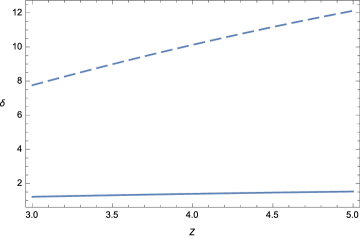
Figure 8: Relative order contributions $\delta$ in percent of vacuum polarization (solid line, order $\alpha^{5}$) and nuclear structure (dashed line, order $\alpha^{5}$) to hyperfine structure of muonic ions of lithium, beryllium and boron.

We present in Tables 2-4 all obtained results for a calculation of corrections in first and second orders of perturbation theory. In the text of our work we give numerous references on that results indicating the lines of Tables 2-4 where these corrections are presented. The dependence of basic corrections of order $\alpha^{5}$ on the nucleus is shown in Fig. 8. As pointed out above the hyperfine structure of muonic ions of lithium, beryllium and boron was investigated previously in drake . The authors of drake gave only estimates of basic contributions in hyperfine structure. In this work we make an attempt to improve their results accounting for different corrections.

The results of calculating various corrections are presented with an accuracy of 0.01 meV. A number of corrections for the polarization of a vacuum have precisely this order. But this does not mean that the accuracy of our calculation is so high. There are already mentioned above corrections to the structure of the nucleus which give the main theoretical uncertainty in the total obtained results. This uncertainty, due to the electromagnetic form factors of the nuclei, can be about 1 percent of the correction to the structure of the nucleus of the order $\alpha^{5}$. Thus, we estimate approximately the errors in the calculation of the HFS spectrum in the form: $\delta E^{hfs}(^{6}_{3}Li)=\pm 1$ meV, $\delta E^{hfs}(^{7}_{3}Li)=\pm 4$ meV, $\delta E^{hfs}(^{9}_{4}Be)=\pm 4.5$ meV, $\delta E^{hfs}(^{10}_{5}B)=\pm 14$ meV, $\delta E^{hfs}(^{11}_{5}B)=\pm 24$ meV. It is appropriate to note here that corrections to the structure of the nucleus of order $\alpha^{5}$ (the Zemach correction) significantly exceed all other corrections listed in the Tables 2-4 (see Fig. 8). We can say that in this respect the hyperfine splitting differs from the Lamb shift $(2P_{1/2}-2S_{1/2})$ in which the correction of the leading order to the structure of the nucleus and the correction for one-loop vacuum polarization are comparable in magnitude and have different signs. Thus, a precise measurement of the HFS in muonic ions of lithium, beryllium and boron, taking into account the obtained theoretical results, will allow obtaining more accurate values of the Zemach radius for these atoms.

There is another correction for the polarizability of the nucleus, which is not considered in this paper. In the case of muonic deuterium, this correction was calculated in ibk1 ; ibk2 . For tritium and helium-3 nuclei, this type of correction was investigated in friar1 . The correction for the polarizability of the nucleus is determined by the interaction of a multinucleon system with an external electromagnetic field, as a result of which the nucleus passes into an excited state. In kp2007 , general expressions were obtained for calculating the various parts of the correction for the nuclear polarizability in the HFS spectrum. Another approach to solving this problem is connected with the use of the dispersion method, in which the correction for the nuclear polarizability is determined by known general formulas and is expressed in terms of the spin-dependent structure functions of the nucleus. If such spin-dependent structure functions of the nuclei were measured exactly experimentally as electromagnetic form factors, then they could be used in calculations. Otherwise, we must consider the motion of the nucleons of the nucleus in the effective potential field and their interaction with an external field. In the case of the Lamb shift, such calculations were performed in bacca . In Refs ibk1 ; friar1 ; kp2007 , the correction for the polarizability in the HFS was discussed together with effects on the structure of the nucleus, so that the total correction was represented in the form: $\delta E^{hfs}=\delta E^{hfs}_{Low}+\delta E^{hfs}_{Zemach}+\delta E^{hfs}_{pol}$. In our approach, in which we use the electromagnetic form factors of the nucleus, the correction for the nuclear structure of order $\alpha^{5}$ (lines 4-5) corresponds to the sum $\delta E^{hfs}_{Low}+\delta E^{hfs}_{Zemach}$, in calculating which the nucleus is represented as the sum of nucleons. The correction for the polarizability is of order $O(Z\alpha m_{1}/m_{2})$, so its possible numerical value for different nuclei (0.6 meV $(^{6}_{3}Li$), 1.8 meV $(^{7}_{3}Li$), -1.6 meV $(^{9}_{4}Be$), 4.7 meV $(^{10}_{5}B$), 7.3 meV $(^{11}_{5}B$)) is comparable in magnitude to those errors that are connected with errors in measuring nuclear form factors. At the same time, it should be noted that the correction for the polarizability for a deuteron substantially exceeds this estimate. Therefore, its exact calculation becomes a very urgent problem. Our work in this direction is in progress.

References

(1)A. Antognini et al., Science 339, 417 (2013).
(2)R. Pohl et al., Science 353, 669 (2016).
(3)B. Franke et al., Eur. Phys. J. D 71, 341 (2017).
(4)R. Pohl, JPS Conf. Proc. 18, 011021 (2017).
(5)A. A. Krutov, A. P. Martynenko, F. A. Martynenko, and O. S. Sukhorukova,
Phys. Rev. A 94, 062505 (2016).
(6)R. Swainson and G. W. F. Drake, Phys. Rev. A 34, 620 (1986).
(7)N. J. Stone, Atomic Data and Nuclear Data Tables 90, 75 (2005).
(8)I. Angeli and K. P. Marinova,Atom. Data Nucl. Data Tabl. 99,
69 (2013).
(9)P. J. Mohr, D. B. Newell and B. N. Taylor, Rev. Mod. Phys. 88, 035009 (2016).
(10)G. Breit, Phys. Rev. 35, 1447 (1930).
(11)M. I. Eides, H. Grotch and V. A. Shelyuto, Phys. Rep. 342, 62 (2001);
Theory of Light Hydrogenic Bound States, Springer Tracts in Modern Physics, V. 222 (Springer, Berlin,
Heidelbeg, New York, 2007).
(12)S. Nozawa and D. B. Leinweber, Phys. Rev. D 42, 3567 (1990).
(13)T. M. Aliev, K. Azizi, and M. Savci, Phys. Lett. B 681, 240 (2009)
(14)S. Deser, A. Waldron and V. Pascalutsa, Phys. Rev. D 62, 105031 (2000).
(15)A. E. Dorokhov, N. I. Kochelev, A. P. Martynenko, F. A. Martynenko, and A. E. Radzhabov,
Eur. Phys. Jour. A 54, 131 (2018).
(16)R. N. Faustov, A. P. Martynenko, G. A. Martynenko and V. V. Sorokin, Phys. Lett. B 733, 354 (2014).