Colour Reconnection from Soft Gluon Evolution

Abstract

We consider soft gluon evolution at the amplitude level to expose the structure of colour reconnection from a perturbative point of view. Considering the cluster hadronization model and an universal Ansatz for the soft anomalous dimension we find strong support for geometric models considered earlier. We also show how reconnection into baryonic systems arises, and how larger cluster systems evolve. Our results provide the dynamic basis for a new class of colour reconnection models for cluster hadronization.

1 Introduction

Multi-purpose Monte Carlo event generators (MCEG) Bahr:2008pv ; Sjostrand:2006za ; Sjostrand:2014zea ; Gleisberg:2008ta play a central role for experimental analyses and phenomenological investigations by simulating particle collisions at a realistic level, including the full complexity and several orders of magnitude difference in relevant energy scales. Starting from a so-called hard scattering at a large momentum transfer, and possibly multiple partonic interactions in hardonic collisions, subsequent radiation in a parton shower is building up the first level of jet substructure and as such provides the first and foremost input to predicting the physical behaviour of observables. These multiple emissions do account for leading logarithmic contributions at all orders of the strong coupling, which can be systematically addressed within analytic approaches to the re-summation of the QCD perturbative series either by the direct analysis of scattering amplitudes and cross sections, or by means of effective field theory methods.

As the typical scales or inter-parton separations reach small scales of the order of $1-2\ {\rm GeV}$, perturbative evolution needs to stop and phenomenological models are used to describe the transition of the partonic ensemble into the observed hadrons. These models take into account non-perturbative corrections, which are included in the analytical approach by means of non-perturbative shape functions, and typically interpret low-mass partonic systems as excited hadronic systems which then break up into stable or unstable hadrons. This applies both to the string hadronization Andersson:1983ia ; Fischer:2016zzs as well as cluster hadronization paradigms Webber:1983if employed in LHC-age MC event generators. The physical picture behind these models is that at the end of the perturbative evolution colour charge is already confined into small phase space regions such that interpretation of excited hadronic systems does make sense, however in the complex and dense environment of hadron-hadron collisions this picture can be spoiled, and is typically invalidated by the presence of multiple partonic scatters.

One therefore expects that further dynamics of exchanging colour charges between the systems are present, which will reduce the relative separations of colour singlet systems. These physics is encoded in colour reconnection models, which are crucial for the description of minimum bias and underlying event data Sjostrand:1993hi ; Lonnblad:1995yk ; Gieseke:2012ft ; Christiansen:2015yca ; Bierlich:2015rha ; Reichelt:2017hts at hadron colliders. The lack of most models to describe baryon production at hadron colliders has also led to improved models of colour reconnection Christiansen:2015yqa ; Gieseke:2017clv .

While the spectrum of colour singlet systems is typically already predicted by the large-$N$ parton shower evolution, the colour reconnection dynamics is a genuine sub-leading-$N$ effect which we expect to be composed of by a perturbative as well as a non-perturbative component. Though the effects have yet only been addressed within the context of non-perturbative models, work is ongoing in analysing multi-parton emission dynamics beyond the leading-$N$ approximation Platzer:2013fha ; Martinez:2018ffw stemming from a detailed analysis of factorisation properties of cross sections, and the resummation of logarithmically enhanced terms. While no consistent connection of such approaches to established hadronization models has been made yet, we take – in this work – the perturbative structure as a starting point to calculate colour reconnecting effects in amplitude level evolution as an input to more constrained, and hence more predictive colour reconnection models.

This paper is organised as follows: In Sec. 2 we review the details of colour pre-confinement and cluster hadronization. Following this in Sec. 3 we introduce the concept of perturbative colour evolution of a scattering amplitude, detailing how different colour structures get mixed in the (infrared) renormalised amplitude by means of a renormalization group equation in colour space. Using this as a proxy to design how a perturbatively inspired colour reconnection model would look like, we state a general algorithm in Sec. 4, where we calculate the probabilities to change from an initial colour flow to a final one by evaluating overlaps of the evolved amplitude and a target colour structure, including baryonic configurations. Sec. 5 analyses in very detail the (exactly solvable) evolution of a two-cluster system in various kinematic regimes and provides an analytic back-up of the dynamics which are typically considered in phenomenological approaches, before we present numerical results for systems of small clusters using a full colour flow evolution in Sec. 6. These results are then considered in Sec. 7 to isolate building blocks for a full-fledged new model of colour reconnection, the implementation of which is subject to ongoing work.

2 Preconfinement and Cluster Hadronization

The cluster hadronization model WEBBER1984492 is an essential ingredient for Monte Carlo Event Generators such as Herwig Bellm:2015jjp and Sherpa Gleisberg:2008ta to convert the partons at scales of the parton shower infrared cutoff of order $1\ {\rm GeV}$ into observed hadrons at energy scales of order $\Lambda_{\text{QCD}}$. The cluster model is based on the property of colour preconfinement AMATI197987 which essentially states that at any scale the colour structure of the parton shower is such that colour singlet combinations of partons can be formed with an asymptotically invariant mass distribution and that this mass distribution is independent of the properties of the hard scattering process or the parton shower itself.

The colour flow of an event is determined through the parton shower, which generally uses the leading colour approximation in order to define the colour flow of a splitting. Since in the large $N$ limit HOOFT1974461 the singlet contribution from emitting gluons is colour suppressed, they can be represented through a colour and an anti-colour line, unambiguously determining the colour flow of a splitting in the parton shower evolution of a state. At the end of the parton shower evolution each coloured parton is colour connected to an anti-coloured parton forming a colour singlet cluster. The properties of a cluster are uniquely defined by the invariant cluster mass

$$M^{2}=\left(p_{q}+p_{\bar{q}}\right)^{2}\ ,$$ (1)

and the kinematics and the flavours of the consitutent quarks ($q$, $\bar{q}$) forming the cluster. Since our analysis will primarily concentrate on the cluster level the specific flavours of the quarks are not of interest and can be neglected. Also for our purposes it is sufficient to stay in the massless parton limit in which Eq. 1 simplifies to $M^{2}=2p_{q}\cdot p_{\bar{q}}$. Mass effects of light quarks are briefly discussed in Sec. 6.4 but not investigated further.

The assignment of colour connections between quark and anti-quark pairs is not without flaws. While at $e^{+}e^{-}$ collisions the colour connections emerging from the parton shower do lead to an asymptotically invariant mass distribution of clusters, the situation becomes ill defined when multiple parton interactions, as they appear during hadronic collisions, are taken into account. Since it is unclear how the colour connections between different scattering centres emerges, non-perturbative models are necessary in order to rearrange the colour flow to arrive at a sensible description of data Sjostrand:1987su . One paradigm which inspired at least the development of one model is the so called notion of a colour pre-confined state which states that after the evolution of the parton shower has terminated, the colour connected partons are close in momentum space leading to a distribution of invariant cluster masses which peaks at small values dictated by the parton shower infrared cutoff. Current developments in this direction, regarding space-time hadronization models are underway and seem to look promising for future studies Ferreres-Sole:2018vgo .

While the bulk of the developments in recent years has been focused more on the non-perturbative modelling side of event generation there hasn’t been much progress on finding further motivation for colour reconnection or rearrangements of colour flows from the perturbative point of view. In this paper we approach this vast topic with a perturbatively inspired evolution of the colour flow due to soft-gluon exchanges and analyse the properties of the resulting cluster configurations which are favoured by our perturbative Ansatz.

3 Perturbative Colour Evolution

QCD scattering amplitudes are vectors in both colour and spin space, and can be decomposed in a basis of contributing colour structures,

$$|{\cal M}\rangle=\sum_{\sigma}{\cal M}_{\sigma}|\sigma\rangle\ ,$$ (2)

where we have suppressed the helicity degrees of freedom as we are mainly interested in the colour structure. These bases are typically over-complete, and non-orthogonal. This poses a computational, but not a conceptual constraint, and in this work we consider the colour flow basis, which at first sight has the worst scaling behaviour in terms of over-completeness, however also exhibits the closest link to the actual flow of colour charge through a scattering amplitude, and provides us with a convenient connection to the parton shower evolution and (pre-)confinement properties. We stress that this basis is not limited to considerations in the large-$N$ limit, and has indeed been shown to be a convenient tool for organising full-colour evolution at the amplitude level Platzer:2013fha ; Martinez:2018ffw , besides its earlier use in the efficient recursive computation of tree-level amplitudes, see e.g. Maltoni:2002mq . Specifically, colour structures in the colour flow basis can be labelled by permutations which describe how colour charge is flowing from one leg to another,

$$|\sigma\rangle=\left|\begin{array}[]{ccc}1&\cdots&n\\ \sigma(1)&\cdots&\sigma(n)\end{array}\right\rangle=\delta^{\alpha_{1}}_{\bar{\alpha}_{\sigma(1)}}\cdots\delta^{\alpha_{n}}_{\bar{\alpha}_{\sigma(n)}}\ .$$ (3)

Virtual corrections are in general both, ultraviolet and infrared divergent. These divergencies are regulated within dimensional regularization, and absorbed into renormalizing bare quantities at a given scale $\mu^{2}$. While ultraviolet divergences in this way relate to the running of the strong coupling, the infrared singularities drive the evolution of a scattering amplitude and the renormalization program in this case can be used to sum large logarithmic contributions of infrared origin to all orders in perturbation theory. To be precise, we can relate the bare amplitude $|\tilde{\mathcal{M}}\rangle$ to the renormalized amplitude $|\mathcal{M}\rangle$ as

$$|\mathcal{M}(\{p\},\mu^{2})\rangle={\mathbf{Z}}^{-1}(\{p\},\mu^{2},\epsilon)|\tilde{\mathcal{M}}(\{p\},\epsilon)\rangle\ ,$$ (4)

where $\{p\}$ is the set of outgoing momenta, $\epsilon=(d-4)/2$ is the dimensional regularization parameter in $d$ dimensions, and $\mu^{2}$ is the scale at which the (infrared) renormalization has been performed. The renormalization constant ${\mathbf{Z}}$ is an operator in the space of colour structures and sums the infrared divergences to all orders, resulting in a finite renormalized amplitude.

By taking a logarithmic derivative of the bare amplitude with respect to $\mu^{2}$ we obtain an evolution equation

$$\mu^{2}\frac{{\rm d}}{{\rm d}\mu^{2}}|{\cal M}(\{p\},\mu^{2})\rangle={\mathbf{\Gamma}}(\{p\},\mu^{2})|{\cal M}(\{p\},\mu^{2})\rangle$$ (5)

where the soft anomalous dimension matrix

$${\mathbf{\Gamma}}(\{p\},\mu^{2})=-{\mathbf{Z}}^{-1}(\{p\},\mu^{2},\epsilon)\mu^{2}\frac{\partial}{\partial\mu^{2}}{\mathbf{Z}}(\{p\},\mu^{2},\epsilon)$$ (6)

encodes the residues of the $1/\epsilon$ divergencies contained in ${\mathbf{Z}}$. At one loop, the soft anomalous dimension reads

$${\mathbf{\Gamma}}(\{p\},\mu^{2})=\sum_{i\neq j}(-{\mathbf{T}}_{i}\cdot{\mathbf{T}}_{j})\Gamma_{\text{cusp}}\ \ln\left(\frac{-s_{ij}}{\mu^{2}}\right)+\sum_{i}\gamma_{i}$$ (7)

where $s_{ij}=2p_{i}\cdot p_{j}$ for two outgoing or two incoming massless partons $i$ and $j$ and $s_{ij}=-2p_{i}\cdot p_{j}$ for incoming/outgoing or outgoing/incoming pairs, and $\Gamma_{\text{cusp}}=\alpha_{s}/4\pi$ in lowest order. The solutions to the evolution equation take the form

$$|{\cal M}(\{p\},\mu^{2})\rangle={\mathbf{U}}(\{p\},\mu^{2},\{M_{ij}^{2}\})|{\cal H}(\{p\},Q^{2},\{M_{ij}^{2}\})\rangle,$$ (8)

where ${\cal{H}}(\{p\},Q^{2},\{M_{ij}^{2}\})$ represents the hard scattering amplitude before the evolution.

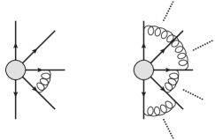
Figure 1: Diagrammatic representation of single soft gluon exchanges between two legs as described by the soft anomalous dimension matrix (left), and all possible iterated exchanges as encoded in the evolution operator (right). Thick lines indicate the momenta of the final state colour charges originating from the hard scattering indicated by the grey blob.

The evolution operator, neglecting the non-cusp terms $\gamma_{i}$ as they are diagonal in colour space, and assuming that only final state, massless partons are present, is

$${\mathbf{U}}\left(\{p\},\mu^{2},\{M_{ij}^{2}\}\right)=\exp\left(-\sum_{i\neq j}\int_{\mu^{2}}^{M_{ij}^{2}}\frac{{\rm d}q^{2}}{q^{2}}(-{\mathbf{T}}_{i}\cdot{\mathbf{T}}_{j})\Gamma_{\text{cusp}}\ \left(\ln\frac{2p_{i}\cdot p_{j}}{q^{2}}-i\pi\right)\right)\ .$$ (9)

Here we have not chosen a fixed scale to provide the initial condition for the evolution but rather have chosen an upper limit on the integration per pair of partons, assuming that $\mu^{2}$ is always less than the scales $M_{ij}^{2}$, which amounts to a specific choice of hard amplitude which is already encoding logarithms of the universal hard scale $Q^{2}$ and the specific mass parameters $M_{ij}^{2}$ which we consider here. The reason for this splitting will soon become clear, however the main point to make here is that the evolution operator ${\mathbf{U}}$ is a matrix exponential in colour space and is describing iterated soft gluon exchanges between any two legs to all orders in the strong coupling. We have illustrated this in Fig. 1.

In terms of the colour flow basis introduced earlier, the action of the evolution operator can be summarised in iterating so-called colour reconnectors Platzer:2013fha which, once per action, will swap two indices of the permutation labelling the specific colour flow, and introduce longer sequences of transpositions when exponentiated. If the colour flows in a basis tensor can be considered to indeed represent physical colour singlet systems, than the evolution operator can be expected to be the basic object describing the physics of colour reconnection at the amplitude level. We shall use this observation as a starting point for our model investigation.

4 The General Algorithm and Baryonic Reconnections

The specific configuration we obtain from a pre-confining parton evolution as discussed in Sec. 2, with a universal cluster mass spectrum, can be seen as driven by a cross section resulting from an amplitude which has been dominated by a colour structure $|\tau\rangle$ corresponding to the assignment of clusters identified in the final state,

$${\rm d}\sigma\sim|{\cal H}(\{p\},Q^{2},\{M_{ij}^{2}\})|^{2}\qquad|{\cal H}(\{p\},Q^{2},\{M_{ij}^{2}\})\rangle\approx{\cal H}_{\tau}(\{p\},Q^{2},\{M_{ij}^{2}\})|\tau\rangle\ .$$ (10)

In this case we assume that the logarithms of $Q^{2}/M_{ij}^{2}$ have been summed by the parton shower evolution with $M_{ij}^{2}\sim 2p_{i}\cdot p_{j}\sim Q_{0}^{2}$, effectively corresponding to a veto of radiation off dipoles with masses around the shower infrared cutoff $Q_{0}^{2}$ and we view the initial step of colour reconnection as an evolution in colour space to scales of order $\mu^{2}$ below the initial cluster masses and the parton shower infrared cutoff. To this extend we identify $M_{ij}^{2}=2p_{i}\cdot p_{j}$, and we use

$${\mathbf{U}}\left(\{p\},\mu^{2},\{M_{ij}^{2}\}\right)=\exp\left(\sum_{i\neq j}{\mathbf{T}}_{i}\cdot{\mathbf{T}}_{j}\frac{\alpha_{s}}{2\pi}\left(\frac{1}{2}\ln^{2}\frac{M_{ij}^{2}}{\mu^{2}}-i\pi\ln\frac{M_{ij}^{2}}{\mu^{2}}\right)\right)$$ (11)

as an Ansatz for the evolution. The starting point for colour reconnection of a cluster configuration represented through a colour structure $|\tau\rangle$ is then to consider the overlap between the evolved amplitude and a new colour structure $|\sigma\rangle$ to constitute a reconnection amplitude,

$${\cal A}_{\tau\to\sigma}=\langle\sigma|{\mathbf{U}}\left(\{p\},\mu^{2},\{M_{ij}^{2}\}\right)|\tau\rangle\ .$$ (12)

Here we have removed the partial amplitude for the colour flow we start to evolve, as it will only an overall normalisation which is irrelevant for the reconnection probability, which we now take to be

$$P_{\tau\to\sigma}=\frac{|{\cal A}_{\tau\to\sigma}|^{2}}{\sum_{\rho}|{\cal A}_{\tau\to\rho}|^{2}}\ ,$$ (13)

where $\rho$ runs over all possible colour flows.

4.1 Baryonic Colour Reconnections

In Gieseke:2017clv the concept of colour reconnection to baryonic clusters has been investigated and proven to be central to the description of baryon production at hadron colliders. In the framework of our perturbatively inspired colour reconnection we can also accommodate for such reconnections provided that there are at least three clusters, or colour flows, to be considered. It is then possible to associate a baryon/anti-baryon pair to a colour structure which has been suitably anti-symmetrized in three fundamental and three anti-fundamental indices

$$|B_{ijk}\rangle=\frac{1}{N_{B}}\epsilon^{ijk}\epsilon_{\bar{i}\bar{j}\bar{k}}=\\ \frac{1}{N_{B}}\left(\left|\begin{array}[]{ccc}i&j&k\\ \bar{i}&\bar{j}&\bar{k}\end{array}\right\rangle+\left|\begin{array}[]{ccc}j&k&i\\ \bar{i}&\bar{j}&\bar{k}\end{array}\right\rangle+\left|\begin{array}[]{ccc}k&i&j\\ \bar{i}&\bar{j}&\bar{k}\end{array}\right\rangle-\left|\begin{array}[]{ccc}j&i&k\\ \bar{i}&\bar{j}&\bar{k}\end{array}\right\rangle-\left|\begin{array}[]{ccc}i&k&j\\ \bar{i}&\bar{j}&\bar{k}\end{array}\right\rangle-\left|\begin{array}[]{ccc}k&j&i\\ \bar{i}&\bar{j}&\bar{k}\end{array}\right\rangle\right)\ .$$ (14)

The normalisation constant is taken to reproduce the normalisation of a single mesonic configuration,

$$\langle B_{ijk}|B_{ijk}\rangle=N^{3}\ ,\qquad N_{B}^{2}=3!\left(1-\frac{3}{N}+\frac{2}{N^{2}}\right)=\frac{4}{3}\ .$$ (15)

This allows us to define a baryonic reconnection amplitude

$${\cal A}_{\tau\to B_{ijk}\otimes\tilde{\sigma}_{ijk}}=\langle B_{ijk}|\otimes\langle\tilde{\sigma}_{ijk}|{\mathbf{U}}\left(\{p\},\mu^{2},\{M_{ij}^{2}\}\right)|\tau\rangle\ ,$$ (16)

where $\tilde{\sigma}_{ijk}$ denotes the permutation with the colour and anti-colour indices corresponding to the baryonic system removed,

$$|\tilde{\sigma}_{ijk}\rangle=\left|\begin{array}[]{cccc}1&\cdots&n&\backslash\ i,j,k\\ \sigma(1)&\cdots&\sigma(n)&\backslash\ \bar{i},\bar{j},\bar{k}\end{array}\right\rangle\ .$$ (17)

The generalised reconnection probability is then

$$P_{\tau\to\sigma}=\frac{|{\cal A}_{\tau\to\sigma}|^{2}}{{\cal N}_{\tau}}\ ,\qquad P_{\tau\to B_{ijk}\otimes\tilde{\sigma}_{ijk}}=\frac{|{\cal A}_{\tau\to B_{ijk}\otimes\tilde{\sigma}_{ijk}}|^{2}}{{\cal N}_{\tau}}$$ (18)

with

$${\cal N}_{\tau}=\sum_{\rho}|{\cal A}_{\tau\to\rho}|^{2}+\sum_{\rho}\sum_{i<j<k}|{\cal A}_{\tau\to B_{ijk}\otimes\tilde{\rho}_{ijk}}|^{2}\ .$$ (19)

We also consider the possibility of evolving an already existing Baryon, for which we introduce ’unbaryonizing’ reconnection amplitudes

$${\cal A}_{B_{ijk}\otimes\tilde{\sigma}_{ijk}\to\tau}=\langle\tau|{\mathbf{U}}\left(\{p\},\mu^{2},\{M_{ij}^{2}\}\right)|B_{ijk}\rangle\otimes|\tilde{\sigma}_{ijk}\rangle\ .$$ (20)

These allow us to quantify how relevant such an evolution step would be for a high-mass baryonic system, which would not have entered the reconnection dynamics any more in the case of the models considered before.

5 A Two-Cluster Sandbox

The goal of this Section is to gain an analytical insight into colour reconnection from soft gluon evolution. In order to do so we study the simplest possible situation of the evolution of a two cluster system. In this case there are just two possible colour flows and according to Eq. 11 the evolution of the single state can be expressed in the following way:

$$|\sigma\rangle={\mathbf{U}}\left|\begin{array}[]{cc}i&j\\ \bar{i}&\bar{j}\end{array}\right\rangle=e^{{\mathbf{\Omega}}}\left|\begin{array}[]{cc}i&j\\ \bar{i}&\bar{j}\end{array}\right>=\sigma_{ij}\left|\begin{array}[]{cc}i&j\\ \bar{i}&\bar{j}\end{array}\right>+\sigma_{ji}\left|\begin{array}[]{cc}j&i\\ \bar{i}&\bar{j}\end{array}\right>\equiv\sigma_{ij}\Ket{ij}+\sigma_{ji}\Ket{ji}$$ (21)

In that case we can provide an explicit expression for the exponent of the evolution operator,

$${\mathbf{\Omega}}=\left(\begin{array}[]{cc}\frac{-3}{2}(\Omega_{23}+\Omega_{14})&\frac{1}{2}(\Omega_{12}-\Omega_{23}-\Omega_{14}+\Omega_{34})\\ \frac{1}{2}(\Omega_{12}-\Omega_{13}-\Omega_{24}+\Omega_{34})&\frac{-3}{2}(\Omega_{13}+\Omega_{24})\end{array}\right)\ ,$$ (22)

where $\Omega_{ij}=\frac{\alpha_{s}}{2\pi}\left(\frac{1}{2}\ln^{2}\frac{M_{ij}^{2}}{\mu^{2}}-i\pi\ln\frac{M_{ij}^{2}}{\mu^{2}}\right)$. However, as will be discussed at the end of Section 6.4 the numerical investigation showed that the Coulomb term in $\Omega_{ij}$ has negligible effect on the massless cluster evolution, which we do not consider in this section for simplicity. We obtain the compact form for $\Omega_{ij}$ in terms of the cluster masses or the partons four-momenta:

$$\Omega_{ij}=\frac{\alpha_{s}}{2\pi}\Big{[}\ln^{2}{\frac{M_{ij}^{2}}{\mu^{2}}}\Big{]}\sim\ln^{2}{{M_{ij}^{2}}}\sim\ln^{2}{2p_{i}\cdot p_{j}}$$ (23)

The evolution is governed by the exponential of the matrix $\mathbf{\Omega}$ which has the structure

$$\mathbf{U}=e^{\mathbf{\Omega}}=\frac{e^{-\frac{3}{2}(a+b)}}{\sqrt{\Delta}}\sinh\left(\frac{\sqrt{\Delta}}{2}\right)\\ \left(\begin{array}[]{cc}\sqrt{\Delta}\coth\left(\frac{\sqrt{\Delta}}{2}\right)+3(b-a)&2(c-a)\\ 2(c-b)&\sqrt{\Delta}\coth\left(\frac{\sqrt{\Delta}}{2}\right)+3(a-b)\\ \end{array}\right),$$ (24)

where we introduced new variables: $a=\ln^{2}\Omega_{23}^{2}+\ln^{2}\Omega_{14}^{2}$, $b=\ln^{2}\Omega_{13}^{2}+\ln^{2}\Omega_{24}^{2}$, $c=\ln^{2}\Omega_{12}^{2}+\ln^{2}\Omega_{34}^{2}$ and $\Delta=9a^{2}-4c(a+b)-14ab+9b^{2}+4c^{2}$. Let us now determine a reconnection probability when the initial colour flow is $\Ket{ij}$:

$$p_{rec}=\frac{|\langle ji|\sigma\rangle|^{2}}{|\langle ji|\sigma\rangle|^{2}+|\left<ij|\sigma\rangle\right|^{2}}\ .$$ (25)

We remind the reader that we work in the basis in which the scalar products are non-orthogonal states and therefore we have $\Braket{ij}{ij}=N^{2}$ and $\Braket{ij}{ji}=N$. Hence $p_{rec}$ can be expressed in terms of evolution matrix $\mathbf{U}$ in the following way:

$$p_{rec}=\frac{|U_{11}+NU_{21}|^{2}}{|NU_{11}+U_{21}|^{2}+|U_{11}+NU_{21}|^{2}}\ ,$$ (26)

where $U_{ij}$ are matrix elements of $\mathbf{U}$. We will now explore properties of $p_{rec}$. The minimal and maximal mixing is obtained at $U_{21}=0$ (with $p_{rec}=\frac{1}{10}$) or $U_{11}=0$ ($p_{rec}=\frac{9}{10}$) respectively, where most of the reconnection values are encountered for extremal cluster mass configurations: In the case when $U_{21}=0$ the condition can be translated to the kinematical situation when masses of final cluster $M_{13}$ and $M_{24}$ fulfil the following equality:

$$U_{21}=0\Leftrightarrow(\ln^{2}M_{12}^{2}+\ln^{2}M_{34}^{2}=\ln^{2}M_{13}^{2}+\ln^{2}M_{24}^{2})\ .$$ (27)

On the other hand in the case $U_{11}=0$ the value of $p_{rec}=\frac{9}{10}$ is obtained when

$$U_{11}=0=\sqrt{\Delta}\coth\left(\frac{\sqrt{\Delta}}{2}\right)+3(b-a)\ .$$

In the limit when $\sqrt{\Delta}$ is large $\coth\left(\frac{\sqrt{\Delta}}{2}\right)\rightarrow 1$ the condition above is much simpler:

$$\frac{3(a-b)}{\sqrt{\Delta}}=0\Leftrightarrow(a-c)(c-b)=0\ .$$

Since we assume that both $U_{11}$ and $U_{21}$ are not equal to $0$ at the same time, the condition above is only fulfilled when

$$a-c=0\Leftrightarrow\ln^{2}M_{23}^{2}+\ln^{2}M_{14}^{2}=\ln^{2}M_{12}^{2}+\ln^{2}M_{34}^{2}\ ,$$

which is also consistent with the numerical results presented in Fig. 15. In general the reconnection probability is bigger than the probability that the system does not change when:

$$p_{rec}>p_{no-rec}\Leftrightarrow U_{21}^{2}>U_{11}^{2}\ ,$$

$$|\sqrt{\Delta}\coth\left(\frac{\sqrt{\Delta}}{2}\right)+3(b-a)|^{2}<|2(c-a)|^{2}\ .$$

Finally, let us cast some light on the rapidity dependence of the result. In order to do it we will work in the frame when particles with four-momenta $p_{1}$ and $p_{2}$ are back-to-back, i.e. $p_{1}=\frac{1}{2}(M_{14},0,0,M_{14})$ and $p_{4}=\frac{1}{2}(M_{14},0,0,-M_{14})$, then for $i=2,3$ we express the four-momenta in the following way: $p_{i}=p_{Ti}(\cosh{y_{i}},\sin{\phi_{i}},\cos{\phi_{i}},\sinh{y_{i}})$. Then the scalar products have the simple form:

$$p_{1}\cdot p_{4}=\frac{1}{2}M_{14}^{2},$$

$$p_{1}\cdot p_{i}=\frac{1}{2}M_{14}p_{Ti}e^{-yi},$$

$$p_{4}\cdot p_{i}=\frac{1}{2}M_{14}p_{Ti}e^{yi},$$

$$p_{2}\cdot p_{3}=2p_{T2}p_{T3}(\cosh{\Delta y_{23}}-\cos{\Delta\phi_{23}}).$$

and the condition for the minimal mixing from Eq. 27 can be rewritten as

$$\ln{\frac{1}{4}M_{14}^{2}p_{T2}^{2}\ln{e^{-2y_{2}}}}=\ln{\frac{1}{4}M_{14}^{2}p_{T3}^{2}\ln{e^{-2y_{3}}}}\ ,$$ (28)

such that, when $p_{T2}\sim p_{T3}$ and $\Delta Y=y_{3}-y_{2}\sim 0$, meaning that the initial partons in clusters have similar transverse momenta and are close in the rapidity, the reconnection mixing is minimal. Therefore, more likely will be reconnections when the $\Delta Y$ values for the quark anti-quark pairs of the original clusters are big, which is also confirmed numerically Fig. 5. It is also interesting to see the transverse momentum dependence of the result from Eq. 28 which we plan to investigate in the future while constructing a phenomenological model based on the current studies.

6 Numerical Results

A significant difference towards other colour reconnection models Gieseke:2012ft ; Gieseke:2017clv is that we do not directly compare clusters and then choose a configuration that would leave us with pre-specified properties such as a lower invariant cluster mass. Since we calculate the probabilities to evolve into different colour flows we first show that our approach leads to reasonable results compatible with the effects of conventional colour reconnection algorithms. In order to analyse the effect of the colour reconnection we mostly compare kinematic variables associated to the clusters before and after reconnection. We first consider ‘mesonic‘ reconnections and later proceed to include ‘baryonic’ reconnections as outlined in Sec. 4.1. We generate initial cluster configurations using the RAMBO method Kleiss:1985gy , and a variation of the Jadach algorithm JADACH1975297 , which was used for the UA5 model ALNER1987445 . While RAMBO is performing a flat phase space population, including a cluster configuration which would not be expected from a pre-confining shower evolution, the UA5 algorithm provides us already with a very physical mass spectrum.

6.1 Mesonic reconnections

A known issue which concerns the modelling of LHC events is that it is a priori not clear how the colour connection between different scattering centres of multi parton interactions looks like. The clusters emerging from these interactions are in general too heavy meaning that they consist of quark anti-quark pairs which are not close in momentum space, in terms of a small invariant mass of the pairs. In this case colour reconnection models are used to restore the notion of a colour pre-confined state leading to a shift towards lower invariant cluster masses. In Fig. 2 we show the invariant mass distribution for five clusters before and after colour reconnection where the phase space was sampled with the two phase space algorithms mentioned above, RAMBO and UA5-type.

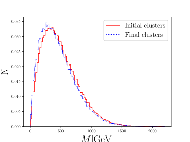
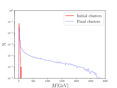
Figure 2: Invariant mass distribution of 5 clusters before and after mesonic colour reconnection for RAMBO(left) and UA5(right) kinematics.

While for the RAMBO kinematics the invariant mass distribution gets shifted towards lower values the clusters generated with the UA5 model already consist of quark anti-quark pairs close in momentum space, which leads to clusters with the smallest invariant mass possible. Considering different colour flows will eventually connect quark anti-quark pairs well separated in rapidity leading to heavier clusters as seen in the right plot of Fig. 2. When sampling the cluster kinematics with the UA5 model but enforcing random colour connections between the quarks and anti quarks for the initial configuration the resulting clusters are large and (in rapidity span) overlapping. A sketch of this configuration is shown in Fig. 3 due to comprehensibility for the simple case of two cluster evolution. For this configuration our Ansatz for colour reconnection again chooses colour flows leading to a shift towards lower values in terms of invariant cluster mass.

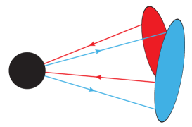
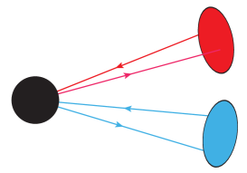
Figure 3: Sketch of the cluster configuration resulting from two alternative colour flows from two cluster evolution. The left figure shows two large overlapping clusters and the right figure shows a different colour flow resulting in smaller clusters consisting of quark anti-quark pairs closer in momentum space. The black blob can be associated with an interaction or parts of an interaction that would lead to the shown configuration.

The effect on the invariant mass spectrum can clearly be seen in Fig. 4, where we plotted the logarithm of the invariant cluster masses.

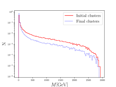
Figure 4: Invariant cluster mass distribution before and after colour reconnection for UA5 kinematics with random initial colour connections.

We conclude that the approach followed in this paper naturally prefers colour flows leading to a configuration with lower invariant cluster masses. We also stress here that the algorithm does not veto any colour flows which would lead to an increase in terms of invariant cluster mass. To get an intuitive picture of what happens on the quark level the rapidity difference, $\Delta Y$, between the quark anti-quark pairs which were participating in the reconnection process is shown in Fig. 5 for the RAMBO phase space and for the UA5 model with random initial colour connections.

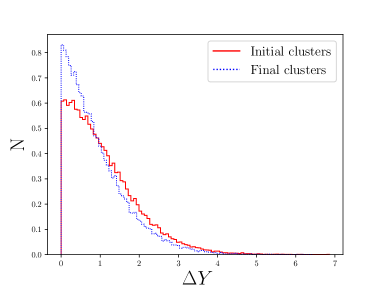
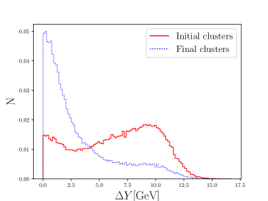
Figure 5: Histogram of the $\Delta Y$ values for the quark anti-quark pairs of the original clusters that were reconnected and the $\Delta Y$ value of the quark anti-quark pairs of the reconnected clusters. (a) RAMBO Phase space. (b) UA5 phase space with random colour connections.

In both figures we see that colour flows resulting in clusters consisting of quark anti-quark pairs which are closer in rapidity are clearly preferred. Again the effect is more pronounced for the UA5 model with random initial colour connections.

6.2 Baryonic reconnections

Within the context of our model a baryonic colour flow can be introduced as explained in Sec. 4.1. In Fig. 6 the average baryonic reconnection probability for both phase space algorithms is shown.

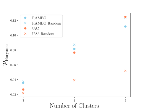
Figure 6: The average baryonic reconnection probabilities for the RAMBO and UA5 phase space option with original and random initial colour connections.

Depending on the phase space algorithm we employ to sample the initial configurations, the average baryonic reconnection probability ranges between $2\%$ and $12\%$. The first striking observation is that the probability rises with the number of clusters considered. The more clusters in an event, the more likely it is to find a candidate for baryonic reconnection. For RAMBO kinematics the initial colour configuration has no effect on the average reconnection probability. For the UA5 phase space it strongly depends on the initial colour configuration. Since the original UA5 cluster configuration already is in a state where the quarks are colour connected to their closest neighbours in phase space the probability for reconnection into a different mesonic state is suppressed, which raises the probability to end up in a baryonic state. If the quarks are randomly connected the average baryonic reconnection probability is suppressed since the probability for mesonic reconnection is high. Also the more clusters we consider, the higher the probability is to find a candidate for baryonic reconnection. Now we proceed to study the three, four and five cluster evolution with the RAMBO phase space in detail. The distribution of the reconnection probabilities is shown in Fig. 7.

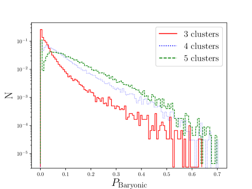
Figure 7: Histogram of baryonic reconnection probabilities for three, four and five cluster evolution where the quark kinematics was sampled with the RAMBO phase space algorithm.

The baryonic reconnection probability tends to prefer lower values with a pronounced peak at zero. The tail towards higher values in the distribution might indicate some preferred kinematic configurations for the evolution into a baryonic state. With only one possible baryonic configuration, the three cluster evolution is convenient to analyse and to extract a kinematic dependence.

In Fig. 8 the probability to evolve into a baryonic state with respect to the sum of average $\Delta R$ values of the quarks and anti-quarks that would constitute a baryonic cluster, $(\langle\Delta R_{B}\rangle+\langle\Delta R_{\bar{B}}\rangle)/2$ is shown, where $\Delta R$ is defined as the distance between the constituent quarks in the $y-\phi$ plane

$$\Delta R=\sqrt{(\Delta\phi)^{2}+(\Delta y)^{2}}.$$ (29)

and we define $\langle\Delta R_{B,\bar{B}}\rangle$ as

$$\langle\Delta R_{B,\bar{B}}\rangle=(\Delta R_{12,\bar{1}\bar{2}}+\Delta R_{13,\bar{1}\bar{3}}+\Delta R_{23,\bar{2}\bar{3}})/3\ ,$$ (30)

where the subscripts $(1,2,3)$, $(\bar{1},\bar{2},\bar{3})$, denote the quarks(anti-quarks) inside the baryonic(anti-baryonic) clusters.

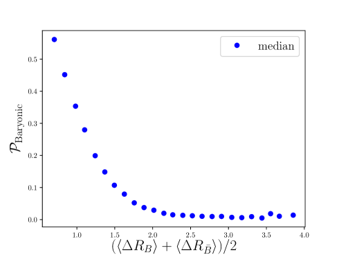
Figure 8: Median values for the baryonic reconnection probability with respect to $(\langle\Delta R_{B}\rangle+\langle\Delta R_{\bar{B}}\rangle)/2$ of the baryonic clusters for 3 cluster evolution.

The median shows a rising probability with lower $(\langle\Delta R_{B}\rangle+\langle\Delta R_{\bar{B}}\rangle)/2$ values which indicates that the formation into a baryonic cluster is preferred if the three quarks and the three anti-quarks are close together in $\Delta R$ space. We note that the baryonic and the anti-baryonic cluster can still be overlapping since we do not take the distance between them into account.

6.3 Unbaryonization

Colour reconnection algorithms that allow reconnection into a baryonic state are structured in a way that once a baryonic cluster is formed, it is not considered for any further modifications. This clearly biases the reconnection procedure but has been necessary in order to cope with the rising complexity of many cluster systems. In principle a system could evolve into a baryonic state and then evolve again into a mesonic state which in turn lowers the amount of baryonic clusters occurring in an event. In the context of our model we can study the evolution back into a mesonic state by considering unbaryonization where we start the evolution with a baryonic configuration as the initial state and calculate the probability to evolve into a mesonic cluster configuration. In Fig. 9 we show the average probabilities for unbaryonization in terms of $(\langle\Delta Y_{B}\rangle+\langle\Delta Y_{\bar{B}}\rangle)/2$ and $(\langle\Delta R_{B}\rangle+\rangle\Delta R_{\bar{B}}\rangle)/2$, where $\langle\Delta Y_{B}\rangle=(|y_{q1}-y_{q2}|+|y_{q1}-y_{q3}|+|y_{q2}-y_{q3}|)/3$. This further adds to the intuitive picture that the probability for forming a baryonic cluster is high if the three quarks and the three anti-quarks are close in momentum space. This also suggests that the colour field between quarks is enhanced if they do fly in the same direction.

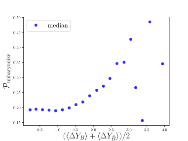
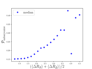
Figure 9: Average unbaryonization probabilities with respect to the average sum of $\langle\Delta Y\rangle$ and $\langle\Delta R\rangle$ of the constituent quarks of the baryonic clusters. The outliers for high values are due to missing statistics.

In principle this could be used in a model such as Gieseke:2017clv to decide whether a baryonic cluster should be kept or not which allows for more flexibility and may un-bias reconnection algorithms.

6.4 Parameter variations and general findings

The Ansatz for the colour flow evolution, Eq. 11 depends on the two parameters $\mu$ and $\alpha_{s}$. Also the so-called Coulomb term proportional to $i\pi$ affects the weights of the different colour flows. The reconnection probability is a dynamic quantity as it strongly depends on the kinematics of the cluster constituents before and after reconnection and the parameter $\mu$ which can be viewed as a cutoff parameter of the colour flow evolution in Eq. 9. In Fig. 10 we show the distribution of invariant cluster masses for four cluster evolution with two different values of $\mu=\{1,0.01\}\,\mathrm{GeV}$ and the corresponding colour length drop Gieseke:2012ft which is defined as

$$\Delta_{\mathrm{if}}=1-\frac{\lambda_{\mathrm{final}}}{\lambda_{\mathrm{initial}}},$$ (31)

where $\lambda_{\mathrm{initial}}$ and $\lambda_{\mathrm{final}}$ denote the colour length before and after colour reconnection in an event which is defined as the sum of squared invariant cluster masses

$$\lambda=\sum_{i=1}^{N_{\mathrm{cl}}}M_{i}^{2}.$$ (32)

If there is no colour reconnection $\lambda_{\mathrm{initial}}\approx\lambda_{\mathrm{final}}$ and $\Delta_{\mathrm{if}}$ approximately vanishes. If $\Delta_{\mathrm{if}}\approx 1$ there was quite a significant change in $\lambda$ which indicates a big effect due to colour reconnection. The kinematics of the four clusters were sampled with the RAMBO method. In order to have more physical cluster masses we sample them with a centre-of-mass energy of $10\,\mathrm{GeV}$ which is closer to the cluster mass spectrum at the end of a typical shower evolution.

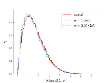
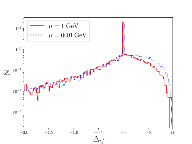
Figure 10: Distribution of invariant cluster masses before and after colour reconnection and colour length drop for different cut-off values of $\mu=\{1,0.01\}\,\mathrm{GeV}$.

Comparing the four cluster evolution with the different values for $\mu$ we see that the lower $\mu$, the more likely it is to pick a colour flow which results in a reduction of invariant cluster masses. For all values the distribution of $\Delta_{\mathrm{if}}$ peaks at zero and is then distributed towards the positive and negative region where the majority of the values are in the positive region indicating a reduction in terms of invariant cluster masses. Negative values of $\Delta_{\mathrm{if}}$ are also possible since we do not veto any colour flows which would result in higher invariant cluster masses. For $\mu=0.01$ the colour reconnection algorithm has the highest impact, severely shifting the distribution of invariant cluster masses towards smaller values which can also be seen for $\Delta_{\mathrm{if}}$. Because $\mu$ can be interpreted as the cut-off parameter of the colour flow evolution if $\mu\rightarrow 0$ the colour flow evolves into a state of preferably low invariant cluster masses.

In Sec 6.1 we showed the effect of the algorithm on a relatively unphysical distribution of cluster masses as a simple proof of concept, that our Ansatz and our algorithm indeed produce reasonable results. In this section we study the evolution of colour flow and the behaviour of the model at different centre-of-mass energies $\sqrt{s}$ with the RAMBO method where we compare $\sqrt{s}=3000\,\mathrm{GeV}$ with a more physical centre-of-mass energy of $\sqrt{s}=10\,\mathrm{GeV}$, probing a spectrum of smaller clusters. We show the reconnection probability for the case of two cluster evolution for the two different centre-of-mass energies with different $\mu$ values in Fig. 11.

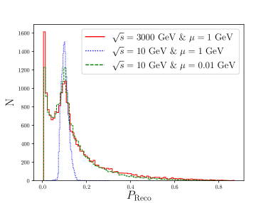
Figure 11: Reconnection probability for the 2 cluster evolution for $\sqrt{s}=3000\,\mathrm{GeV}$ and $\sqrt{s}=10\,\mathrm{GeV}$.

While at $\sqrt{s}=3000\,\mathrm{GeV}$ the reconnection probability covers the whole range from zero to one, at $\sqrt{s}=10\,\mathrm{GeV}$ and $\mu=1\,\mathrm{GeV}$ they are narrowly distributed around $0.1$. With $\mu=1\,\mathrm{GeV}$ for small centre-of-mass energies the values are closer together which leads to similar reconnection probabilities in each event. This can be countered by reducing the $\mu$ parameter such that the ratio in the logarithm is the same as for higher energies which is also shown in Fig. 11 for the two cluster evolution with $\sqrt{s}=10\,\mathrm{GeV}$ and $\mu=0.01\,\mathrm{GeV}$.

With a smaller $\mu$ parameter the reconnection probabilities start to cover the whole range, and we observe the same behaviour for baryonic reconnections. The smaller the value of $\mu$ the amplitude in colour space will continue to evolve down to a much smaller scale which, in the end will result in a colour flow with preferably small invariant cluster masses. In a full model the parameter $\mu$ could be tuned to data in order to define the cutoff at which the evolution is bound to stop and to verify if the amplitude does indeed favour a state of small invariant cluster masses or a state which allows for more fluctuations in terms of cluster size.

Another interesting topic is the mass distributions for different centre of mass energies. In Fig. 12 we show the mass distributions of four clusters for $10\,\mathrm{GeV}$ and $3000\,\mathrm{GeV}$ divided by the centre-of-mass energy with the possibility to produce baryonic clusters.

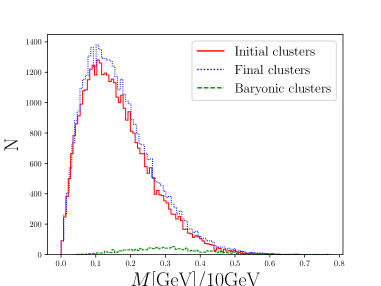
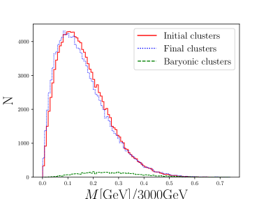
Figure 12: Distribution of invariant cluster masses for $\sqrt{s}=10\,\mathrm{GeV}$ and $\sqrt{s}=3000\,\mathrm{GeV}$ divided by their respective $\sqrt{s}$.

The distributions of the reconnected clusters are roughly the same although for $10\,\mathrm{GeV}$ there is much less room to evolve into a state of smaller cluster masses since we used $\mu=1\,\mathrm{GeV}$. The mass distribution of baryonic clusters is also shifted between the two centre of mass energies. Since the soft anomalous dimension matrix only depends on the ratio of the invariant cluster masses and the cut off parameter $\mu$, it is possible to find an energy independent prescription which should lead to the same distribution of cluster masses.

A continuation of the arguments of the logarithms towards very small cluster masses, $\ln(\frac{M_{\alpha\beta}^{2}}{\mu^{2}})\to\ln(\frac{M_{\alpha\beta}^{2}}{\mu^{2}}+1)$ has been considered but did not show any change in our findings and can as such be used to prevent numerical instabilities should the relevant small masses be encountered in a full model. The strong coupling parameter $\alpha_{s}$ is clearly a direct measure of the overall reconnection strength and while we have chosen it to reflect the strong coupling at a lowish scale, $\alpha_{s}=0.118$, it should, in practice also be considered a tunable parameter of the model.

Until now we neglected quark masses completely, which lead to the simplified form of the invariant cluster mass. Assuming the same quark (constituent) masses for light quarks ($0.3$ GeV for up and down quarks) , which are used in the cluster hadronization model, only small effects were found in terms of the mass distribution and no sizeable effects on the reconnection probabilities. For heavy quarks ($m_{b}\sim 4-5\mathrm{GeV}$) more severe effects are expected but we leave this topic for a detailed study in the scope of a full-fledged model implementation. Switching off the Coulomb term does not change our findings for the high-mass systems, while we see some effects for small-mass systems.

7 Towards a Full Model

Due to its complexity, the approach followed in this paper is limited to a small number of clusters and should be seen as a theoretical consideration to constrain the structure of an improved colour reconnection model. It clearly makes a full colour flow evolution un-feasible to implement on the typically large systems of clusters encountered in a typical high energy collisions. We will mainly use the insights we gained from looking at evolution of small systems to extrapolate a simplified model which could be suitable for implementation. A crucial aspect is to identify independently evolving subsystems in the cases with the highest number of clusters we did consider here. This will allow us to formulate ‘microscopic’ input to a model iterating over small numbers of clusters within a large ensemble.

The cluster configurations, being essentially colour structures in the colour flow basis, can be labelled by permutations and an important question to ask is what the minimum number of transpositions one requires to transform the initial configuration into a final, reconnected configuration. This number is directly related to the power of the number of colours $N$ when evaluating the overlap between the two colour structures, with more transpositions leading to a higher $1/N$ suppression. In Fig. 13 we show the number of transpositions for four and five cluster evolution where the phase space was populated with the RAMBO method.

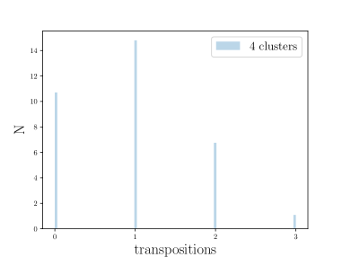
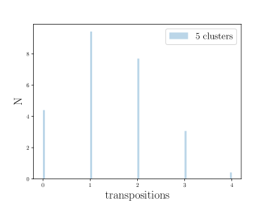
Figure 13: Number of transpositions between the initial state and the reconnected final state for four and five cluster evolution.

For both cases we note the peak at one transposition, i.e. a reconnection within a two cluster system, between the initial and final state. This indicates the existence of independently evolving subsystems where the contributions from the remainder of the event are suppressed. Crucially, this indicates that colour reconnection is not simply a $1/N$ suppressed effect which would have indicated a much higher rate of non-reconnected systems, as well as a much steeper drop of the other reconnection dynamics with the number of transpositions. Our finding is then also indicative of a choice of evolving small subsystem out of a larger configuration as depicted in Fig. 14, where mixing with well separated clusters can actually be neglected.

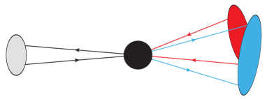
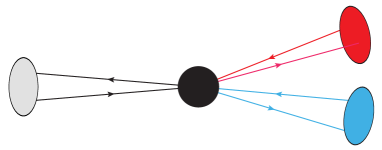
Figure 14: Sketch of a configuration where the two coloured clusters could be viewed as an independently evolving subsystem. Gluon exchanges which would lead to colour connections with the grey cluster are expected to be highly suppressed. Left: Initial colour flow. Right: Colour flow after reconnection.

Colour reconnection models implemented in event generators often rely on very simplified models in order to handle the complex structure of hadronic collisions. In an old model in the Herwig event generator, for example, reconnections would only be accepted if they allowed for a smaller mass configuration, and with a fixed probability which essentially was inferred by tuning to underlying event data. While this approach has benefits in terms of efficiency and simplicity, and has shown to provide a reasonable description of data Gieseke:2012ft it does not take into account the full kinematic dynamics and complexity of a hadronic event.

In order to make contact with this simple model, and to highlight the fact that geometric models as well as the non-trivial kinematic dependence of our Ansatz provide a much more dynamic model, we consider the reconnection probability projected to the variable of the old model, which essentially is the ratio of the sum of cluster masses before and after reconnection. Having generated kinematics of two clusters with the RAMBO algorithm with $\sqrt{s}=10\,\mathrm{GeV}$, $\mu=0.01\,\mathrm{GeV}$, $\alpha_{s}=0.118$ and for comparison with $\sqrt{s}=3000\,\mathrm{GeV}$, $\mu=1\,\mathrm{GeV}$, $\alpha_{s}=0.118$ to visualise the energy dependence, and plot the median of the reconnection probabilities over the ratio of the sum of invariant cluster masses, which would result from the two different possible colour flows, see Fig. 15.

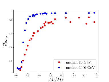
Figure 15: Parametrisation of the reconnection probability for two cluster evolution in terms of the ratio of invariant cluster masses $M_{i}/M_{f}$, where $M_{i}$ is the sum of invariant cluster masses of the initial colour flow and $M_{f}$ is the sum of invariant cluster masses of the alternative colour flow of a two cluster system.

The old model would here only have put a step function in place, with no further kinematic dependence present. We also stress the fact that the reconnection probability does not vanish, but saturates at $\approx 0.9$ if reconnection would result in a lower sum of invariant cluster masses and mounts up at $\approx 0.1$ if $M_{i}=M_{f}$ or $M_{i}<M_{f}$. These limits can already be obtained from our analytic studies in Sec. 5. For both energies it is clear that the dependence of the reconnection probability on the ratio of cluster masses is a more dynamical one than a simple step function.

We therefore suggest to indeed use our findings as an input to more sophisticated reconnection models along the lines of Gieseke:2017clv :

• The analytically known reconnection probability from the evolution of two cluster systems can, with the finding of mostly independently evolving two cluster systems, be used directly to improve the model assumption of these type of reconnections.

• The fact that also three cluster systems seem to be rather detached in a large ensemble can be used to supplement the baryon production mechanism in Gieseke:2017clv with a more dynamic reconnection probability, possibly based on approximating this evolution to the first few orders in a $1/N$ expansion Platzer:2013fha .

• The baryonic reconnection mechanism, which has so far not considered the possibility of un-connecting baryonic clusters in an evolution picture or statistical model Gieseke:2012ft .

All of these mechanisms are contained within our approach and that such a model will be highly predictive in the sense that with the analogue of the strong coupling $\alpha_{s}$ and the soft scale $\mu$ it contains effectively two, possibly three parameters if one wants to include the number of colours $N$, as well. We finally note that, though we have essentially been considering the cluster hadronization model in our considerations, a similar dynamics could be implemented in a string picture.

8 Conclusions and Outlook

We have studied to what extent the structure of perturbative colour evolution can be used as an input to improve or constrain existing colour reconnection models. In particular, we have analytically solved the evolution of a two-cluster system, as well as numerically studied the evolution of larger systems of up to five clusters. We have found that there is indeed a highly dynamic and non-trivial re-arrangement of colour structures already from a simple Ansatz using a one-loop soft anomalous dimension, which confirms earlier work on geometrically inspired reconnection models Gieseke:2017clv .

The full evolution in colour space is, however, not feasible in a realistic model which needs to cope with several tens to hundreds of clusters. However we have found evidence that in the evolution of larger systems the bulk of the reconnection effects is isolated in small subsystems of two to three clusters which allow to build an iterative model, which can also be based on approximations of the evolution operator Platzer:2013fha . Our framework also allows to include a probability of re-connecting baryonic clusters into mesonic systems, an important aspect which has not been considered in models of baryonic reconnection so far, but could result in a detailed balance mechanism to establish a realistic fraction of baryons for given partonic constituent dynamics.

We stress the fact that our approach should not only be considered as a motivation for improved models of non-perturbative colour reconnection but does highlight that the perturbative mixing of colour structures, mediated through virtual soft gluon exchanges, should be considered an important ingredient in new approaches to improving parton shower algorithms beyond the leading-$N$ level Martinez:2018ffw , and that these effects are in general not mediated in a probabilistic manner, or through tree-level amplitudes. However until such algorithms are fully available, and the dynamics of hadronization is understood in this context, we postpone further aspects to future work and use the findings obtained here as an improved input to existing colour reconnection models.

References

- (1) M. Bähr et al., Herwig++ Physics and Manual, Eur. Phys. J. C58 (2008) 639–707, [0803.0883].
- (2) T. Sjöstrand, S. Mrenna and P. Z. Skands, PYTHIA 6.4 Physics and Manual, JHEP 05 (2006) 026, [hep-ph/0603175].
- (3) T. Sjöstrand, S. Ask, J. R. Christiansen, R. Corke, N. Desai, P. Ilten et al., An Introduction to PYTHIA 8.2, Comput. Phys. Commun. 191 (2015) 159–177, [1410.3012].
- (4) T. Gleisberg, S. Höche, F. Krauss, M. Schönherr, S. Schumann, F. Siegert et al., Event generation with SHERPA 1.1, JHEP 02 (2009) 007, [0811.4622].
- (5) B. Andersson, G. Gustafson, G. Ingelman and T. Sjöstrand, Parton Fragmentation and String Dynamics, Phys. Rept. 97 (1983) 31–145.
- (6) N. Fischer and T. Sjöstrand, Thermodynamical String Fragmentation, JHEP 01 (2017) 140, [1610.09818].
- (7) B. R. Webber, A QCD Model for Jet Fragmentation Including Soft Gluon Interference, Nucl. Phys. B238 (1984) 492–528.
- (8) T. Sjöstrand and V. A. Khoze, On Color rearrangement in hadronic W+ W- events, Z. Phys. C62 (1994) 281–310, [hep-ph/9310242].
- (9) L. Lönnblad, Reconnecting colored dipoles, Z. Phys. C70 (1996) 107–114.
- (10) S. Gieseke, C. Rohr and A. Siódmok, Colour reconnections in Herwig++, Eur. Phys. J. C72 (2012) 2225, [1206.0041].
- (11) J. R. Christiansen and T. Sjöstrand, Color reconnection at future e+ e- colliders, Eur. Phys. J. C75 (2015) 441, [1506.09085].
- (12) C. Bierlich and J. R. Christiansen, Effects of color reconnection on hadron flavor observables, Phys. Rev. D92 (2015) 094010, [1507.02091].
- (13) D. Reichelt, P. Richardson and A. Siódmok, Improving the Simulation of Quark and Gluon Jets with Herwig 7, Eur. Phys. J. C77 (2017) 876, [1708.01491].
- (14) J. R. Christiansen and P. Z. Skands, String Formation Beyond Leading Colour, JHEP 08 (2015) 003, [1505.01681].
- (15) S. Gieseke, P. Kirchgaeßer and S. Plätzer, Baryon production from cluster hadronisation, Eur. Phys. J. C78 (2018) 99, [1710.10906].
- (16) S. Plätzer, Summing Large- Towers in Colour Flow Evolution, Eur. Phys. J. C74 (2014) 2907, [1312.2448].
- (17) R. A. Martinez, M. De Angelis, J. R. Forshaw, S. Plätzer and M. H. Seymour, Soft gluon evolution and non-global logarithms, 1802.08531.
- (18) B. Webber, A qcd model for jet fragmentation including soft gluon interference, Nuclear Physics B 238 (1984) 492 – 528.
- (19) J. Bellm et al., Herwig 7.0/Herwig++ 3.0 release note, Eur. Phys. J. C76 (2016) 196, [1512.01178].
- (20) D. Amati and G. Veneziano, Preconfinement as a property of perturbative qcd, Physics Letters B 83 (1979) 87 – 92.
- (21) G. ’t Hooft, A planar diagram theory for strong interactions, Nuclear Physics B 72 (1974) 461 – 473.
- (22) T. Sjöstrand and M. van Zijl, A Multiple Interaction Model for the Event Structure in Hadron Collisions, Phys. Rev. D36 (1987) 2019.
- (23) S. Ferreres-Solé and T. Sjöstrand, The Space-Time Structure of Hadronization in the Lund Model, 1808.04619.
- (24) F. Maltoni, K. Paul, T. Stelzer and S. Willenbrock, Color flow decomposition of QCD amplitudes, Phys. Rev. D67 (2003) 014026, [hep-ph/0209271].
- (25) R. Kleiss, W. J. Stirling and S. D. Ellis, A New Monte Carlo Treatment of Multiparticle Phase Space at High-energies, Comput. Phys. Commun. 40 (1986) 359.
- (26) S. Jadach, Rapidity generator for monte-carlo calculations of cylindrical phase space, Computer Physics Communications 9 (1975) 297 – 304.
- (27) G. Alner et al., The UA5 high energy pp simulation program, Nuclear Physics B 291 (1987) 445 – 502.