Krylov projection methods for linear Hamiltonian systems

Abstract

We study geometric properties of Krylov projection methods for large and sparse linear Hamiltonian systems. We consider in particular energy-preservation. We discuss the connection to structure preserving model reduction. We illustrate the performance of the methods by applying them to Hamiltonian PDEs.

1 Introduction

Large and sparse linear Hamiltonian systems arise in many fields of science and engineering, examples are models in network dynamics van2014port and the semi-discretization of Hamiltonian partial differential equations (PDEs), like the wave equation feng1987symplectic ; mclachlan1993symplectic and Maxwell’s equations marsden1982hamiltonian ; sun10sam . In the context of Hamiltonian PDEs, the energy conservation law often plays a crucial role in the proof of existence and uniqueness of solutions taylor115partial . Energy-preservation under numerical discretization can be advantageous as it testifies correct qualitative behaviour of the numerical solution, and it is also useful to prove convergence of numerical schemes richtmyer1967difference . There is an extensive literature on energy-preserving methods for ordinary differential equations (ODEs) labudde1975energy ; mclachlan1999geometric ; brugnano10hbv ; celledoni2012preserving , but these methods need to be implemented efficiently to be competitive for large and sparse systems arising in numerical PDEs. Krylov projection methods are attractive for discrete PDE problems because they are iterative, accurate and they allow for restart and preconditioning strategies. But their structure preserving properties are not completely understood and should be further studied.

It is well known that integration methods cannot be simultaneously symplectic and energy-preserving on general Hamiltonian systems ge88lph . However, the situation changes when we restrict to linear systems. An example is the midpoint rule which is symplectic and is also energy-preserving on linear problems because it coincides with the AVF method quispel08anc . The midpoint method is implicit and requires the solution of one linear system of algebraic equations at each time step. The structure preserving properties are then retained only to the precision of the linear iterative solver. In this paper, we investigate preservation of geometric properties in Krylov projection methods. These are attractive methods for the solution of large systems arising in PDEs botchev2009numerical , but because of the Krylov projection, symplecticity is only preserved to the accuracy of the method. On the other hand, we show that some of these methods can be energy-preserving to a higher level of precision, and can preserve several first integrals simultaneously. We finally discuss the connections to structure-preserving model reduction and variational principles. Previous work in the context of structure preserving Krylov projection methods can be found in lopez2006preserving ; MR3126684 and for Hamiltonian eigenvalue problems for example in benner98ans .

The structure of this paper is as follows. We discuss symplecticity in section 2. Section 3 is devoted to the preservation of first integrals. Section 4 is devoted to projection methods based on block $J$-orthogonal bases and their connection to structure preserving model reduction. In Section 5, the geometric properties of the considered methods are illustrated by numerical examples.

2 Krylov projection and symplecticity

Consider a linear Hamiltonian initial value problem of the form

$$\dot{y}=JH\,y,\quad y(0)=y_{0},\hskip 56.9055ptJ=J_{m}=\left[\begin{matrix}0&I_{m}\\ -I_{m}&0\end{matrix}\right],$$ (1)

where $y(t)\in\mathbb{R}^{2m}$, $H\in\mathbb{R}^{2m\times 2m}$ is symmetric, $y_{0}\in\mathbb{R}^{2m}$, and $I_{m}$ is the $m\times m$ identity matrix. In what follows we denote by $A$ the product $A=JH$. The skew-symmetric matrix $J$ defines a symplectic inner product on $\mathbb{R}^{2m}$, $\omega(x,y):=x^{T}Jy.$ The vector field of equation (1) is a Hamiltonian vector field. The flow of a Hamiltonian vector field is a symplectic map. This means that $\varphi_{t}:\mathbb{R}^{2m}\rightarrow\mathbb{R}^{2m}$, $y_{0}\mapsto y(t)$, is such that $\Psi_{y_{0}}(t)=\frac{\partial\varphi_{t}(y_{0})}{\partial y_{0}}$ satisfies

$$\Psi_{y_{0}}(t)^{T}\,J\,\Psi_{y_{0}}(t)=J.$$ (2)

In other words, $\Psi_{y_{0}}(t)$ is an element of the symplectic group $\mathrm{Sp}(2m)$, and $y(t)=\Psi_{y_{0}}(t)y_{0}$. Crucially, any element of $U\in\mathrm{Sp}(2m)$ is such that the change of variables $x=Uy$ sends Hamiltonian systems to Hamiltonian systems. Denote by $\mathcal{H}(y)=\frac{1}{2}{y}^{T}J^{-1}Ay$ the energy function. Another fundamental property of the system (1) is that $\mathcal{H}$ is constant along solution trajectories, i.e., $\frac{d\,\mathcal{H}(y(t))}{dt}=0.$ An approximation method for (1) is said to be energy-preserving if $\mathcal{H}$ is constant along the numerical solution, and symplectic if the numerical flow $\phi_{h}:\mathbb{R}^{2m}\rightarrow\mathbb{R}^{2m}$, $y_{0}\mapsto\tilde{y}$ with $\tilde{y}\approx y(h)$, is such that $\frac{\partial\phi_{h}(y_{0})}{\partial y_{0}}^{T}J\frac{\partial\phi_{h}(y_{0})}{\partial y_{0}}=J.$

The idea of Krylov projection methods is to build numerical approximations for (1) in the Krylov subspace:

$$\mathcal{K}_{r}(A,y_{0}):=\mathrm{span}\{y_{0},Ay_{0},\cdots,A^{r-1}y_{0}\},$$

which is a subspace of $\mathbf{R}^{2m}$ of dimension $r<<2m$. Let us consider even dimension $r=2n$. A basis of $\mathcal{K}_{2n}(A,y_{0})$ is constructed. The most well known Krylov projection method is the one based on the Arnoldi algorithm arnoldi1951principle generating an orthonormal basis for $\mathcal{K}_{2n}(A,y_{0})$. The method gives rise to a $2m\times 2n$ matrix $V_{2n}$ with orthonormal columns, and to an upper Hessenberg $2n\times 2n$ matrix $H_{2n}$ such that $I_{2n}={V_{2n}}^{T}V_{2n},$ and $H_{2n}=V_{2n}^{T}AV_{2n}.$ The approximation of $y(t)$ is

$$y_{A}:=V_{2n}z(t),\quad\mathrm{where}\quad\dot{z}=H_{2n}\,z,\quad z(0)=z_{0}=V_{2n}^{T}y_{0}.$$ (3)

We will denote this method by Arnoldi projection method (APM). Consider $J_{2n}$ and the symplectic inner product in $\mathbb{R}^{2n}$, $\bar{\omega}(\bar{x},\bar{y})=\bar{x}^{T}J_{2n}\bar{y}$. If $n<m$, unless we make further assumptions on $H$, the projected system (3) is not a Hamiltonian system in $\mathrm{R}^{2n}$, this can be seen because $J_{2n}^{-1}H_{2n}=J_{2n}^{-1}V_{2n}^{T}JHV_{2n}$ is in general not symmetric.

Instead of using an orthonormal basis, one can construct a $J$-orthogonal basis for $\mathcal{K}_{2n}(A,y_{0})$ using the symplectic Lanczos algorithm benner2011hamiltonian . The matrix $S_{2n}$ whose columns are the vectors of this $J$-orthogonal basis satisfies

$$S_{2n}^{T}JS_{2n}=J_{2n}.$$

We will denote the corresponding Krylov projection method by Symplectic Lanczos projection method (SLPM). The projected system for SLPM is analog to (3), with $V_{2n}$ replaced by $S_{2n}$, $H_{2n}$ by $J_{2n}S_{2n}^{T}HS_{2n}$ and an appropriate $z_{0}$ (see Section 3.3). This projected system is a Hamiltonian system. But for $n<m$, the approximation $y_{S}(t):=S_{2n}z(t)$ is not symplectic. In fact, $y_{S}$ is the solution of the system

$$\dot{y}_{S}=(S_{2n}J_{2n}S_{2n}^{T})\,H\,y_{S},\quad y_{S}(0)=y_{0},$$ (4)

which is a Poisson system with Poisson structure given by the skew-symmetric matrix $(S_{2n}J_{2n}S_{2n}^{T})$ which depends on the initial condition. For $n=m$, $S_{2m}\in\mathrm{Sp}(2m)$, $J_{2m}=J$, and $y_{S}=y.$ However, the case $n<m$ is the most relevant for the use of the method in practice. In spite of not preserving $\omega$, SLPM clearly shares important structural properties with the exact solution of (1) and is energy-preserving, see Section 3.3.

The symplectic Lanczos algorithm is not the only way to obtain a $J$-orthogonal basis of the Krylov subspace. We will consider block $J$-orthogonal bases in Section 4 and show that they can be viewed as techniques of structure preserving model reduction, in the spirit of lall2003structure . We propose one Krylov algorithm based on these ideas.

3 Preservation of first integrals and energy

We first present a result about the first integrals for a general linear Hamiltonian system.

Proposition 1

For $A=JH$ where $J$ is skew symmetric and invertible, and $H$ is symmetric and invertible, the system $\dot{y}=Ay$, $y(0)=y_{0}$ has $m$ independent first integrals in involution, $\mathcal{H}_{k}(y)=\frac{1}{2}\langle y,A^{2k}y\rangle_{H}$ for $k=0,1,\dots,m-1$. The Hamiltonian of the system is $\mathcal{H}=\mathcal{H}_{0}$.

Proof

We have

$$\frac{d}{dt}\mathcal{H}_{k}(y) = \frac{1}{2}\left[\dot{y}^{T}H(JH)^{2k}y+y^{T}H(JH)^{2k}\dot{y}\right]$$

$$= \frac{1}{2}\left[-y^{T}HJH(JH)^{2k}y+y^{T}H(JH)^{2k}JHy\right]$$

$$= \frac{1}{2}\left[-y^{T}H(JH)^{2k+1}y+y^{T}H(JH)^{2k+1}y\right]=0,$$

so $\mathcal{H}_{k}$, $k=0,\dots,m-1$ are preserved along solutions of $\dot{y}=Ay$, $y(0)=y_{0}$. The integrals are in involution because their Poisson bracket is zero,

$$\{\mathcal{H}_{k},\mathcal{H}_{p}\} =(\nabla\mathcal{H}_{k})^{T}J\nabla\mathcal{H}_{p}=y^{T}((JH)^{2k})^{T}HJH(JH)^{2p}y$$

$$=y^{T}H(JH)^{2(k+p)+1}y=0,$$

where we have used the skew-symmetry of $H(JH)^{2(k+p)+1}$. The integrals are functionally independent because, when $J$ and $H$ are invertible, $J^{-1}\nabla\mathcal{H}_{k}=2J^{-1}A^{2k}y$ for $k=0,\dots,m-1$ are linearly independent vectors

In what follows, we will discuss the preservation of the first integrals of Proposition 1 when applying Krylov projection methods.

3.1 Preservation of first integrals for the APM

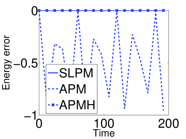
It can be observed from numerical simulations that the APM fails in general to preserve energy when applied to Hamiltonian systems, Figure 1(a), Section 5, but structure-preserving properties can be ensured for such method via a simple change of inner product. Assume that $H$ is symmetric and positive definite so that $\langle\cdot,\cdot\rangle_{H}:=\langle\cdot,H\cdot\rangle$ defines an inner product. We modify the Arnoldi algorithm by replacing the usual inner product $\langle\cdot,\cdot\rangle$ by $\langle\cdot,\cdot\rangle_{H}$. We then show that the numerical solution given by this method preserves to machine accuracy certain first integrals. The modified Arnoldi algorithm (see Algorithm 2) generates a $H$-orthonormal basis, which is stored in the $2m\times n$ matrix $V_{n}$, satisfying $V_{n}^{T}HV_{n}=I_{n}$. This algorithm generates an upper Hessenberg matrix $H_{n}$ such that

$$\begin{split}AV_{n}&=V_{n}H_{n}+w_{n+1}e_{n}^{T},\quad w_{n+1}=h_{n+1,n}v_{n+1},\\ {V_{n}}^{T}HV_{n}&=I_{n},\quad{V_{n}}^{T}Hw_{n+1}=0.\end{split}\vspace{-10pt}$$

In what follows, we consider the Krylov projection method

$$y_{H}:=V_{n}z,\quad\mathrm{where}\,\,z\,\,{\mathrm{satisfies}}\quad\dot{z}=H_{n}\,z,\quad z(0)={V_{n}}^{T}Hy_{0}.$$

Proposition 2

The numerical approximation $y_{H}$ for the solution $y$ of (1) preserves the following first integrals:

$$\mathcal{H}_{k}(y_{H})=\frac{1}{2}y_{H}^{T}HV_{n}(H_{n})^{2k}{V_{n}}^{T}Hy_{H}$$ (5)

for all $k=0,1,\dots,r$, where $r=[\frac{n}{2}]-1$.

Proof

We observe that $H_{n}={V_{n}}^{T}HJHV_{n}$ is skew-symmetric. So the ODE system for $z$ has first integrals: $\mathcal{I}_{k}(z)=\frac{1}{2}z^{T}(H_{n})^{2k}z$, for all $k=0,1,\dots,r$ with $r=n/2-1$ if $n$ is even and $r=(n-1)/2-1$ if $n$ is odd. Therefore $\mathcal{H}_{k}(y_{H})=\frac{1}{2}y_{H}^{T}HV_{n}(H_{n})^{2k}{V_{n}}^{T}Hy_{H}=\frac{1}{2}z^{T}(H_{n})^{2k}z$ are preserved.

Remark 1

If $n$ is even, the above Krylov projection method induces a projected problem which is conjugate to a Hamiltonian system, i.e., it can be written in the form (1) via change of variables. Since $H_{n}$ is skew-symmetric, $H_{n}$ can be factorized as $H_{n}=U_{n}J_{n}D_{n}U_{n}^{-1}$ where $D_{n}$ is diagonal. Then, $H_{n}$ can be transformed to a Hamiltonian matrix by a similarity transformation using $U_{n}$.

3.2 Hamiltonian system with $JA=AJ$

We now consider $J$ given by (1). Assume that $A$ and $J$ commute, then $A$ is skew-symmetric, and the Hamiltonian system (1) has two Hamiltonian structures, one associated to $A$ with Hamiltonian $\frac{1}{2}y^{T}y$, the other to $J$ with Hamiltonian $\frac{1}{2}y^{T}Hy$. The APM with Euclidean inner product $\langle\cdot,\cdot\rangle$ preserves modified first integrals. To proceed, we first give without proof the following result.

Proposition 3

Suppose $A$ is a Hamiltonian matrix. Then $J$ and $A$ commute if and only if the matrix $A$ is skew-symmetric.

The first integrals of the system (1) are given by the following proposition.

Proposition 4

If $JA=AJ$, the Hamiltonian system (1) has $m$ independent first integrals in involution, $\mathcal{H}_{k}(y)=\frac{1}{2}y^{T}A^{2k}y$ for $k=0,1,\dots,m-1$, and in involution with the Hamiltonian $\mathcal{H}(y)=\frac{1}{2}y^{T}Hy$.

Proof

From Proposition 3 we know that $A$ is skew-symmetric. Then Proposition 1 holds with $J$ replaced by $A$, and $H$ replaced by the identity matrix. The integrals are in involution with the Hamiltonian $\mathcal{H}(y)=\frac{1}{2}y^{T}Hy$ in fact using the commutativity of $A$ and $J$

$$\{\mathcal{H}_{k},\mathcal{H}\}=y^{T}A^{2k}JAy=y^{T}A^{k}(JA)A^{k}y=0,\quad k=0,\dots,m-1.$$

Remark 2

By a direct application of Proposition 2, the APM to the Hamiltonian system (1), under the assumption $JA=AJ$, gives a numerical approximation $y_{A}:=V_{n}z$ which preserves the following modified first integrals

$$\mathcal{\tilde{H}}_{k}(y_{A}):=\frac{1}{2}y_{A}^{T}V_{n}(H_{n})^{2k}V_{n}^{T}y_{A},\quad k=0,1,\dots,n.$$

We next prove that the Hamiltonian of (1) is bounded by $y_{A}$ under the assumption that $J$ and $A$ commute.

Proposition 5

Assume the APM is applied to (1). Under the assumption $JA=AJ$, the energy $\mathcal{H}(y)=\frac{1}{2}{y}^{T}J^{-1}Ay,$ is bounded along the numerical solution.

Proof

This result follows directly from Remark 2 with $k=0$, i.e.,

$$\frac{1}{2}{y_{A}}^{T}J^{-1}Ay_{A}\leq\frac{1}{2}{y_{A}}^{T}y_{A}\|J^{-1}A\|_{2}=\frac{1}{2}{y_{0}}^{T}y_{0}\|J^{-1}A\|_{2}.$$

Proposition 5 explains the good behaviour of the APM in celledoni16epk .

3.3 Symplectic Lanczos projection method

We now introduce the symplectic Lanczos projection method (SLPM). For this method the projected system (3) is a Hamiltonian system. We prove that the SLPM preserves the energy of the original system.

Given $A\in R^{2m,2m}$ and the starting vector $y_{0}\in R^{2m}$, the symplectic Lanczos method generates a sequence of matrices

$$S_{2n}=[v_{1},...,v_{n},w_{1},...w_{n}]\quad\mathrm{satisfying}\quad AS_{2n}=S_{2n}H_{2n}+r_{n+1}e^{T}_{2n},$$ (6)

where $H_{2n}$ is a tridiagonal Hamiltonian matrix, and $r_{n+1}=\zeta_{n+1}v_{n+1}$ is $J$-orthogonal with respect to the columns of $S_{2n}$. Since $S_{2n}$ has $J$-orthogonal columns, i.e., ${S_{2n}}^{T}JS_{2n}=J_{2n}$, we know that

$$H_{2n}=J_{2n}^{-1}\,S_{2n}^{T}JAS_{2n}=J_{2n}S_{2n}^{T}HS_{2n},$$ (7)

and the projected system is a Hamiltonian system, where $z_{0}=J_{2n}^{-1}S_{2n}^{T}Jy_{0}$. Moreover, we have

$$\mathcal{H}_{S}(z)=\frac{1}{2}z^{T}J_{2n}^{-1}H_{2n}z\equiv\frac{1}{2}z_{0}^{T}J_{2n}^{-1}H_{2n}z_{0}.$$ (8)

Proposition 6

The SLPM is an energy-preserving method for (1).

Proof

The result follows by computing the Hamiltonian of (1) along numerical trajectories $y_{S}=S_{2n}z$, $\mathcal{H}(y_{S})=\frac{1}{2}{y_{S}}^{T}J^{-1}Ay_{S},$ and then using (6) and (8).

4 Projection methods based on block $J$-orthogonal basis

We now consider a general strategy for Krylov projection methods to obtain $J$-orthogonal bases. In what follows we will use the notation $(q^{T},p^{T})^{T}=y$ and write $H$ in block form, and rewrite (1) accordingly:

$$\begin{split}\dot{q}&=H_{12}^{T}q+H_{22}p,\\ \dot{p}&=-H_{11}q-H_{12}p,\end{split}\qquad\quad H=\begin{bmatrix}H_{11}&H_{12}\\ H_{12}^{T}&H_{22}\end{bmatrix}.$$ (9)

Assume that we can construct two matrices with linearly independent columns $V_{n}\in{\mathbb{R}}^{m\times n}$ and $W_{n}\in{\mathbb{R}}^{m\times n}$ such that ${V_{n}}^{T}W_{n}=I_{n}$. Then the matrix

$$S_{2n}:=\begin{bmatrix}V_{n}&0\\ 0&W_{n}\end{bmatrix}$$ (10)

has $J$-orthogonal columns. We will approximate $y$ by the following projection method: $y\approx y_{B}$ defined by

$$y_{B}=S_{2n}\,z,\quad\mathrm{where}\,\,z\,\,{\mathrm{satisfies}}\quad\dot{z}=J_{2n}\,S_{2n}^{T}J^{-1}AS_{2n},\quad z(0)=z_{0},$$ (11)

and for the SLPM $z_{0}=J_{2n}^{-1}S_{2n}^{T}Jy_{0}$.

Proposition 7

If $y_{0}=S_{2n}z(0)$, then the energy of the original Hamiltonian system (1) will be preserved by the numerical solution (10)-(11).

Proof

Notice that $\mathcal{H}(S_{2n}\,z)=\frac{1}{2}z^{T}S_{2n}^{T}J^{-1}AS_{2n}\,z$ is a constant because $z$ is the solution of a Hamiltonian system with energy $\mathcal{K}(z)=\frac{1}{2}z^{T}(S_{2n}^{T}J^{-1}AS_{2n})\,z$. The result then follows directly from the fact that $\mathcal{K}(z)\equiv\mathcal{K}(z_{0})=\mathcal{H}(y_{0})$.

We here propose one strategy to construct $S_{2n}$ as in (10) with $W_{n}^{T}V_{n}=I_{n}$ and $V_{n}=W_{n}$. Let $K_{n}$ be the Krylov matrix $2m\times n$, and consider the first $m$ rows of $K_{n}$ and the last $m$ separately:

$$K_{n}:=[y_{0},Ay_{0},\dots,A^{n-1}y_{0}],\qquad K_{n}=\left[\begin{array}[]{c}K_{n}^{q}\\[5.69046pt] K_{n}^{p}\end{array}\right].$$

We then find an orthonormal basis $V_{n}$ for $\mathrm{span}\{K_{n}^{q},K_{n}^{p}\}\subset\mathbb{R}^{m}$ by either a QR-factorisation (algorithm 2 in the Appendix ) or a Gram-Schmidt process.

4.1 Structure preserving model reduction using Krylov subspaces

In this section we consider the variational principle lying behind the presented techniques. This allows to draw connections to the techniques of structure preserving model reduction of lall2003structure , see also peng2016symplectic . Assuming additional structure for $H$, we will also show that the usual APM applied to the resulting system coincides with a structure preserving model reduction method.

Assume $[q^{T},p^{T}]^{T}:=y$ and $q$ and $p$ are $m$-dimensional vectors belonging to $\mathbf{R}^{m}$ and its dual respectively, and that the Hamiltonian $\mathcal{H}:\mathbf{R}^{m}\times(\mathbf{R}^{m})^{*}\rightarrow\mathbf{R}$ is $\mathcal{H}(q,p):=\mathcal{H}(y).$ Considering the action functional $\mathcal{S}:\mathbf{R}^{m}\times(\mathbf{R}^{m})^{*}\rightarrow\mathbf{R}$

$$\mathcal{S}(q,p):=\int_{t_{0}}^{t_{end}}\left({p(t)}^{T}\dot{q}(t)-\mathcal{H}(q(t),p(t))\right)\,dt,$$

Hamilton’s phase space variational principle states that

$$\delta\mathcal{S}=0$$

for fixed $q_{0}=q(t_{0})$ and $q_{end}=q(t_{end})$, and it is equivalent to Hamilton’s equations (1). By projecting $q(t)$ and $p(t)$ separately on appropriate subspaces $\mathrm{span}\{V_{n}\}\subset\mathbf{R}^{m}$ and $\mathrm{span}\{W_{n}\}\subset(\mathbf{R}^{m})^{*}$, i.e., $q(t)\approx V_{n}\,\hat{q}(t)$ and $p(t)\approx W_{n}\,\hat{p}(t)$, one restricts the variational principle to $\mathrm{span}\{V_{n}\}\times\mathrm{span}\{W_{n}\}$: $\hat{\mathcal{S}}(\hat{q},\hat{p}):=\mathcal{S}(V_{n}\,\hat{q},W_{n}\,\hat{p}).$ By taking variations

$$0=\delta\hat{\mathcal{S}}(\hat{q},\hat{p})=\delta\int_{t_{0}}^{t_{end}}(V_{n}\hat{p})^{T}W_{n}\dot{\hat{q}}(t)-H(V_{n}\hat{p},W_{n}\hat{q})dt$$

for fixed endpoints $\hat{q}_{0}=\hat{q}(t_{0})$ and $\hat{q}_{end}=\hat{q}(t_{end})$, we obtain the Hamiltonian equations associated to this reduced variational principle

$$\begin{split}\dot{\hat{p}}&=-{V_{n}}^{T}{H_{12}}W_{n}\hat{p}-{V_{n}}^{T}H_{11}V_{n}\hat{q},\\ \dot{\hat{q}}&={W_{n}}^{T}H_{22}W_{n}\hat{p}+{W_{n}}^{T}H_{12}^{T}V_{n}\hat{q},\end{split}$$ (12)

which coincide with the system for $z$ in (11).

4.2 Special case $H_{1,2}=O$, $H_{2,2}=I$.

This special case is directly related to the setting in lall2003structure . Denoting $y=(q^{T},p^{T})^{T}$, we consider the action functional associated to the Lagrangian

$$L(q(t),\dot{q}(t))=\frac{1}{2}{\dot{q}(t)}^{T}\dot{q}(t)-\frac{1}{2}{q(t)}^{T}H_{11}q(t)$$ (13)

and the corresponding Hamiltonian system

$$\dot{y}=Ay\quad\text{with}\quad A=\begin{bmatrix}0&I\\ -H_{11}&0\end{bmatrix}.$$ (14)

Let $V_{n}$ be the basis of the Krylov subspace $\mathcal{K}_{n}(-H_{11},p_{0})$ obtained via the Arnoldi algorithm. The reduced Lagrangian becomes

$$L(\hat{q}(t),\dot{\hat{q}}(t))=\frac{1}{2}{\dot{\hat{q}}(t)}^{T}\dot{\hat{q}}(t)-\frac{1}{2}{\hat{q}(t)}^{T}{V_{n}}^{T}H_{11}V_{n}\hat{q}(t),$$ (15)

and the corresponding Hamiltonian equations are

$$\begin{split}\dot{\hat{q}}&=\hat{p},\\ \dot{\hat{p}}&=-{V_{n}}^{T}H_{11}V_{n}\hat{q}(t).\end{split}$$ (16)

By solving (16), we obtain $(\hat{q}^{T},\hat{p}^{T})^{T}$ and then can construct the model reduction approximation $((V_{n}\hat{q})^{T},(V_{n}\hat{p})^{T})^{T}\approx(q^{T},p^{T})^{T}$.

Proposition 8

When applied to (14) with $y_{0}=(0,p_{0}^{T})^{T}$, the model reduction procedure outlined in (13)-(16) coincides with the APM.

Proof

Let $\mathbf{e}_{1},\mathbf{e}_{2}\in\mathbf{R}^{2}$ be the two vectors of the canonical basis in $\mathbf{R}^{2}$. Denote by $\otimes$ the Kronecker tensor product. We have

$$\mathcal{K}_{2n}(A,y_{0})=\mathrm{span}\{\mathbf{e}_{1}\otimes p_{0},\mathbf{e}_{2}\otimes p_{0},\mathbf{e}_{1}\otimes(-H_{11}p_{0}),\mathbf{e}_{2}\otimes(-H_{11})p_{0},\dots\}.$$

Denote by $\mathbb{U}_{2n}\in{\mathbb{R}}^{2m\times 2n}$ the orthogonal matrix generated by the usual Arnoldi algorithm with matrix $A$, vector $y_{0}=(0,p_{0}^{T})^{T}$ and Euclidean inner product. Then $\mathbb{U}_{2n}$ is given by

$$\mathbb{U}_{2n}=\left[\begin{array}[]{cccccccc}0&v_{1}&0&v_{2}&0&\dots&0&v_{n}\\ v_{1}&0&v_{2}&0&v_{3}&\dots&v_{n}&0\end{array}\right],$$

and satisfies

$${\mathbb{U}_{2n}}^{T}A\mathbb{U}_{2n}=\Pi_{2n}\begin{bmatrix}0&I_{n}\\ -V_{n}^{T}H_{11}V_{n}&0\end{bmatrix}{\Pi_{2n}}^{T}\quad\mathrm{and}\quad\mathbb{U}_{2n}\Pi_{2n}=\left[\begin{array}[]{cc}V_{n}&O\\ O&V_{n}\end{array}\right],$$

where $v_{1},v_{2},\dots v_{n}$ are the columns of $V_{n}$ and $\Pi_{2n}$ is a $2n\times 2n$ permutation matrix. After a permutation of the variables $w={\Pi_{2n}}^{T}z$, the projected system by APM $\dot{z}={\mathbb{U}_{2n}}^{T}A\mathbb{U}_{2n}z$, $z(0)={\mathbb{U}_{2n}}^{T}y_{0}$ can be rewritten in the form (10)-(11).

5 Numerical Examples

In this section, several numerical examples are presented to illustrate the behavior of the methods described above. We will use the following methods:

• APM: Arnoldi projection method using Euclidean inner product, Section 3;

• APMH: Arnoldi projection method using the inner product $\langle\cdot,\cdot\rangle_{H}$, Section 3;

• SLPM: symplectic Lanczos projection method, Section 3.3;

• BJPM: block $J$-orthogonal projection method QR factorization, Section 4.1.

These methods are applied to solve randomly generated linear Hamiltonian systems, and linear systems arising from the discretization of Hamiltonian PDEs.

5.1 Randomly generated Hamiltonian matrices

We consider numerical experiments on randomly generated linear Hamiltonian systems. If not mentioned otherwise, the dimension of the Krylov subspace is chosen to be $2n=4$ and is the same for all the Krylov methods compared. The reference exact solution is computed using the Cayley transformation with step-size $0.004$. The solution of the projected system (3) is obtained with the same approach and step-size used for the reference exact solution. To obtain a desired global error accuracy on $[0,T]$ for large $T$, we either use a sufficiently large dimensions of the Krylov subspace or perform a restart procedure using the Krylov projection methods on sufficiently small subintervals. More precisely, the considered restart procedure consists in subdividing $[0,T]$ into subintervals $[t_{k},t_{k+1}]$ and performing the projection on each subinterval recomputing the basis of the Krylov subspace with starting vector $y_{k}$, where $y_{k}$ is the numerical solution at $t=t_{k}$. The restart procedure is of practical interest because it allows to use a Krylov subspace of low dimension. However, the restart destroys the preservation of the first integrals of Propositions 2 and 4 for APM and APMH because the basis $V_{n}$ is recomputed on each subinterval. Experiments comparable to the ones performed in this section can be found in peng2016symplectic for model reduction techniques without restart.

5.1.1 Case $JA=AJ$: APM

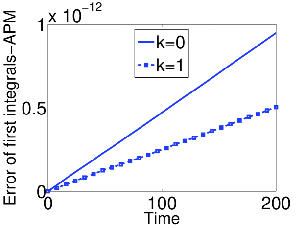
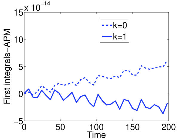
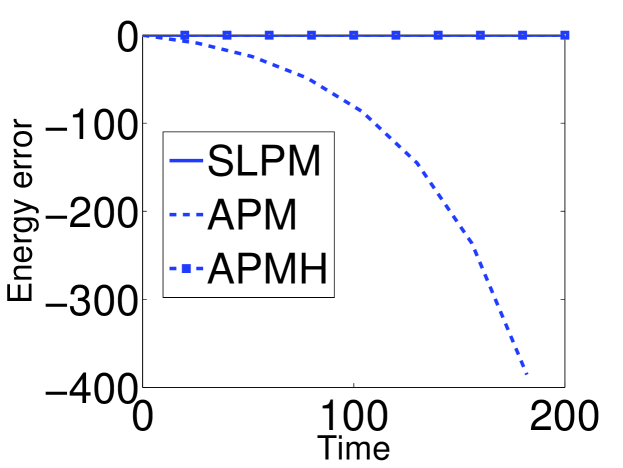
In the experiments reported in Figure 1(a), $H=J^{-1}A$ is block diagonal, symmetric and positive definite but with no particular extra structure. We observe in Figure 1(a) that there is a drift in the energy for the APM, and the advantage of APMH and SLPM is evident in this example. The global errors are not reported here, but we find that the global errors of APMH and SLPM are bounded, meanwhile there is a substantial drift in the global error of the APM in this case. In Figure 1(b) and 1(c), we apply the APM to an example where $JA=AJ$. The experiments confirm the good behaviour of the APM in this case. Figure 1(b) shows that the energy error for the APM is bounded even though the energy is not preserved exactly. The global error, which we do not report here, is also bounded for all three methods in this example. For such matrices, we observe in Figure 1(c) that the two first integrals of Proposition 2 for $k=0$ and $k=1$ are preserved for the APM, see also Remark 2.

(a) Energy error

(b) Energy error

(c) First integrals, APM

Figure 1: Methods without restart. In Figure 1(a) a block diagonal Hamiltonian matrix is considered. In Figure 1(b) and 1(c), we consider a skew-symmetrix, Hamiltonian matrix $A$.

5.1.2 Full matrices: Comparison of APMH, SLPM, BJPM

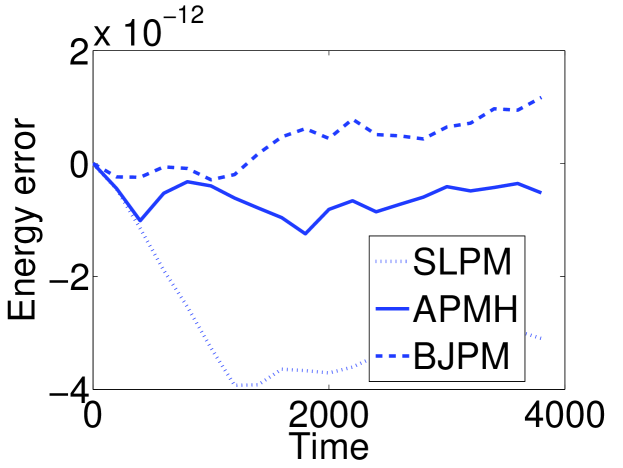
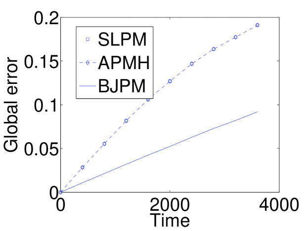
In this subsection, we consider a randomly generated, full Hamiltonian matrix $A=JH$. In Figure 3, we use the methods without restart. Figure  3(a) shows that the first integrals of Proposition 2 are preserved by APMH on a moderately large time interval and for a general Hamiltonian matrix (i.e. imposing only that $JA$ is symmetric). However, even if the error is of size $10^{-14}$, there is a clear drift in the first integrals. A similar drift is observed also in the energy error for all methods without restart. In Figure 2 we use the restart technique. The energy is well preserved for all three methods, the global error grows slowly and linearly (and it remains bounded also for larger times intervals). Here and in other experiments, the BJPM perform better in the energy error and global error compared to the other considered methods. As previously mentioned, the restart procedure destroys the preservation of first integrals of Proposition 2.

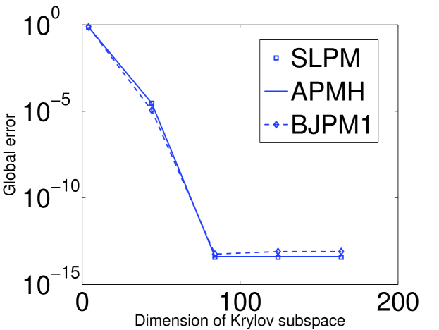
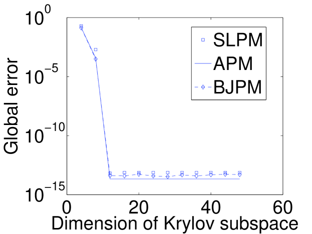
In Figure 3(b), we report convergence plots for APMH, SLPM and BJPM, showing how the global error decreases when the dimension of the Krylov subspace increases and the end time $T$ is fixed. We observe that the global error decreases to almost $10^{-15}$, and all the methods converge. $T$ is equal to $2$ in this experiment, but the methods converge well also for larger end time, such as $T=200$.

(a) Energy error

(b) Global error

Figure 2: Methods with restart.

(a) First integrals, APMH

(b) Convergence

Figure 3: Methods without restart. In Figure 3(b), the global error at the end time $T=2$ is shown.

5.1.3 Case $H_{1,2}=O$, $H_{2,2}=I$: Model reduction

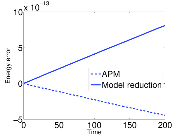
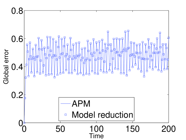
In Figure 4, we consider a Hamiltonian matrix $A$ of the special form (14) with an initial vector of the form $y_{0}=(0,p_{0}^{T})^{T}$. We use the Arnoldi algorithm with matrix $-H_{11}$ and vector $p_{0}$ to generate the orthogonal matrix $V_{n}$ in the model reduction procedure described in Section 4.2. The methods behave as predicted. The APM behaves very well in this case and similarly to the methods based on model reduction, see Sec 4.2. Energy preservation is shown in Figure 4(a) and bounded numerical error is shown in Figure 4(b). Notice that we cannot apply the restart technique in this case because the special form of the initial vector will in general not be maintained from the first to the second subinterval.

(a) Energy error

(b) Global error

Figure 4: APM compared to a procedure of model reduction.

5.2 Hamiltonian PDEs

In this section we apply the methods to the wave equations and the Maxwell’s Equations.

5.2.1 Wave equation

We consider the $2\mathrm{D}$ wave equations

$$\dot{\phi}=\psi,\qquad\dot{\psi}=\triangle\phi,$$ (17)

on $[0,1]\times[0,1]$ with homogeneous Dirichlet boundary conditions $\phi(t,0,y)=\phi(t,1,y)=\phi(t,x,0)=\phi(t,x,1)=0$ and a randomly generated initial vector. Semi-discretizing on an equispaced grid $x_{i}=i\,\Delta x$ and $y_{j}=j\,\Delta y$, $\Delta x=\Delta y$, $i,j=0,\dots,N$ and assuming $u(x_{i},y_{j})\approx U_{i,j}$, we obtain a system

$$\dot{U}=AU,\quad U(0)=U_{0},\qquad A=\left[\begin{matrix}0&I\\ G&0\end{matrix}\right]$$ (18)

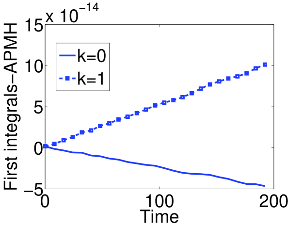
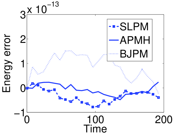
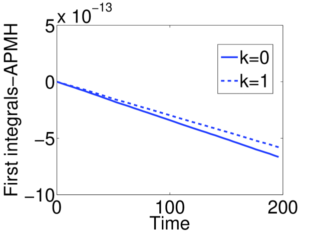
with $G$ the discrete 2D Laplacian obtained by using central differences. This is a Hamiltonian system with energy $\mathcal{H}=\frac{1}{2}U^{T}JAU\equiv\frac{1}{2}U(0)^{T}JAU(0).$ We perform experiments with all the Krylov projection methods discussed in this paper. Figure 5(a) shows that all the methods are energy-preserving. Figure 5(b), shows that first integrals are preserved by APMH.

(a) Energy error

(b) First integrals-APMH

(c) Global error-APMH

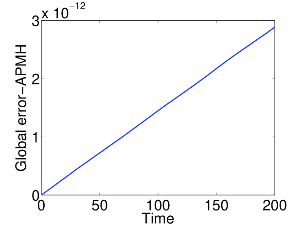
Figure 5: Wave equation in $2d$. Figure 5(a) energy error, methods with restart. Figure 5(b), first integrals, methods without restart. Maxwell’s equations in $1$d, Figure 5(c), global error, methods without restart.

5.2.2 $1\mathrm{D}$ Maxwell’s equations

We consider $1\mathrm{D}$ Maxwell’s equations

$$\begin{split}\partial_{t}E&=\partial_{x}B,\\ \partial_{t}B&=\partial_{x}E\end{split}$$ (19)

for $x\in[0,1]$ and $t>0$ with boundary conditions $E(0,t)=E(1,t)=0,\,B_{x}(0,t)=B_{x}(1,t)=0$ and initial conditions $E(x,0)=\sin(\pi x)$ and $B(x,0)=\cos(\pi x)$. After semi-discretization with $E(x_{i},t)\approx E_{i}(t)$ and $B(x_{i},t)\approx B_{i}(t)$, $i=0,\dots,N$, we get a system of ODEs

$$\dot{U}=\bar{S}DU,\quad U(0)=U_{0},$$ (20)

where $U=[E_{1},...,E_{N-1},B_{0},...,B_{N}]^{T}$ and

$${\small\bar{S}=\frac{1}{2h}\left[\begin{matrix}0_{N-1,N+1}&G\\ \vspace{4mm}\\ -G^{T}&0_{N+1,N-1}\end{matrix}\right]},\qquad{\small G=\left[\begin{matrix}-2&0&1&&\\ \vspace{1mm}&-1&0&1&\\ \vspace{1mm}&&\ddots&\ddots&\ddots&\\ \vspace{1mm}&&&-1&0&1\\ \vspace{1mm}&&&&-1&0&&2\end{matrix}\right]}$$

and $D=\mathrm{diag}(I_{N-1},\frac{1}{2},I_{N-1},\frac{1}{2})$. Equation (20) fits the framework of section 3, with $\bar{S}$ skew-symmetric and $D$ symmetric and positive definite, therefore APMH can be applied to this problem. The numerical approximation of $U$ obtained applying the APMH preserves the first integrals $\mathcal{H}_{k}(\bar{U})$ of Proposition 2. The first integrals are preserved with an error of about $10^{-13}$ (not reported here). In Figure 5(c), we show the global error and observe that the problem is solved with high accuracy.

5.3 Numerical results for $3\mathrm{D}$ Maxwell’s equations

We consider $3\mathrm{D}$ Maxwell’s equations in CGS units for the electromagnetic field in a vacuum

$$\begin{split}\partial_{t}E&=-c\nabla\times B,\\ \partial_{t}B&=c\nabla\times E.\end{split}$$ (21)

The boundary conditions are zero and the initial conditions are randomly generated for both fields. We consider $c=1$. We get the following Hamiltonian system after semi-discretization:

$$\dot{U}=AU,\qquad U(0)=U_{0},$$

$$A=\left[\begin{matrix}0&-G_{1}\\ G_{1}&0\end{matrix}\right],$$ (22)

where $U=[E_{1,1,1},...,E_{N-1,N-1,N-1},B_{1,1,1},...,B_{N-1,N-1,N-1}]^{T}$ and $G_{1}$, symmetric and of the size $(N-1)^{3}$, is the discretization of the curl operator $\nabla\times$.

Remark 3

The matrix $A$ is skew-symmetric in equation (22). Therefore the APMH with $J=A,H=I$ applied to the system (22), equals the APM and preserves the first integrals $\mathcal{H}_{k}(\bar{U})$ of Proposition 2.

Remark 4

Equation (22) can be rewritten as a Hamiltonian equation $\dot{U}=JHU,$ with $H=J^{-1}A$ a symmetric matrix. Therefore we can also apply SLPM and BJPM to system (21) and the energy $\mathcal{H}(U)=\frac{1}{2}U^{T}J^{-1}AU$ is preserved. However, APMH cannot be used here because $H$ is not a positive definite matrix, and the inner product $\langle\cdot,\cdot\rangle_{H}$ is degenerate. This can lead to instabilities and both global error and energy error might blow up during the iteration.

(a) Energy error

(b) Energy error, BJPM

(c) Global error, BJPM

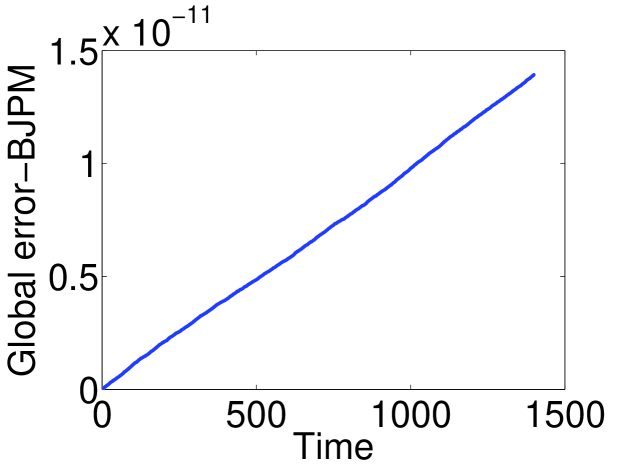
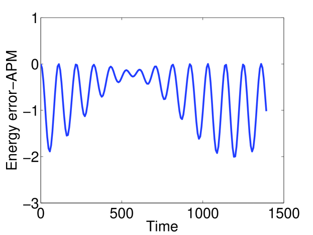
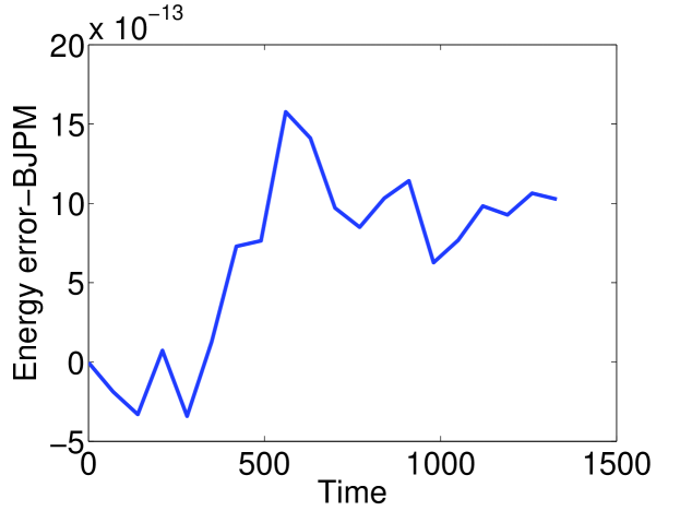
Figure 6: The dimension of Krylov subspace is set to be $4$ in Figure 6(a) and $16$ in Figure 6(b) and 6(c). In Figure 6(b) and 6(c), the methods with the restart technique are used. Figure 6(a) corresponds to the energy error considered as in Remark 3, while figure 6(b) to the energy error considered in Remark 4.

(a) First integrals-APM

(b) Convergence

Figure 7: In Figure 7(a), the dimension of Krylov subspace is set to be $4$. In Figure 7(b) we consider $L^{2}$ norm of the global error at $t=T=2$ as a function of the dimension of the Krylov subspace.

Figure 6(a) shows that the energy error of APM is bounded as stated in Remark 3. The energy error of APM will decrease to $10^{-12}$ when we increase the dimension of the Krylov subspace from $4$ to $16$ (not shown here). Figure 6(b) shows that the energy $\mathcal{H}(U)=\frac{1}{2}U^{T}J^{-1}AU$ is preserved for BJPM as stated in Remark 4. The problem is solved to high accuracy by BJPM with dimension of Krylov space $16$. As shown in Figure 7(a), APM preserves the first integrals in Remark 3. In Figure 7(b), we report convergence plots for the methods. As the dimension of the Krylov subspace increases, the global error decreases very fast for all the methods.

6 Appendix

.5

1:Input: a matrix $J\in{\mathbb{R}}^{m\times m}$, $H\in{\mathbb{R}}^{m\times m}$, a vector $b\in\mathbb{R}^{m}$, a number $n\in\mathbb{N}$ and a tolerance $\iota\in\mathbb{R}$.

2:$A=JH$ 

3:$v_{1}=\frac{b}{\langle b,b\rangle_{H}^{\frac{1}{2}}}$ 

4:for $j=1:n$ do

5:     compute $w_{j}=Av_{j}$ 

6:     for $k=1:2$ do

7:         for $i=1:j$ do

8:              $h_{i,j}=\langle v_{i},w_{j}\rangle_{H}$ 

9:              $w_{j}=w_{j}-h_{i,j}v_{i}$ 

10:         end for

11:     end for

12:     $h_{j+1,j}=\langle w_{j},w_{j}\rangle_{H}^{\frac{1}{2}}$ 

13:     if $h_{j+1,j}<\iota$ then

14:         Stop

15:     end if

16:     $v_{j+1}=w_{j}/h_{j+1,j}$ 

17:end for

18:Output: $H_{n},V_{n},v_{n+1},h_{n+1,n}$.

Table 1: Arnoldi’s algorithm with modified inner product

.5

1:Matrix $A\in{\mathbb{R}}^{2m\times 2m}$, vector $b\in{\mathbb{R}}^{2m}$, number $n\in\mathbb{N}$.

2:$v=b$ 

3:$K_{n}=v$ 

4:for $i=1:n-1$ do

5:     $v=Av$ 

6:     $K_{n}=[K_{n},v]$ 

7:end for

8:$K_{n}^{q}=K_{n}(1:m,:)$ 

9:$K_{n}^{p}=K_{n}(m+1:2m,:)$ 

10:$[Q,R]=qr([K_{n}^{q},K_{n}^{p}])$ 

11:$V_{n}=Q(:,1:k),\quad k=\mathrm{rank}([K_{n}^{q},K_{n}^{p}])\leq 2n$ 

12:Output $V_{n}$.

Table 2: Algorithm to generate $V_{n}$ (by QR factorization)

References

• (1) A. van der Schaft, D. Jeltsema, Port-Hamiltonian systems theory: An introductory overview, Foundations and Trends in Systems and Control 1(2-3), 173 (2014)
• (2) K. Feng, M.z. Qin, in Numerical methods for partial differential equations (Springer, 1987), pp. 1–37
• (3) R. McLachlan, Symplectic integration of Hamiltonian wave equations, Numerische Mathematik 66(1), 465 (1993)
• (4) J.E. Marsden, A. Weinstein, The Hamiltonian structure of the Maxwell-Vlasov equations, Physica D: nonlinear phenomena 4(3), 394 (1982)
• (5) Y. Sun, P. Tse, Symplectic and multisymplectic methods for Maxwell’s equations, J. Comp. Phys. 230(5), 2076 (2010). DOI 10.1016/j.jcp.2010.12.006
• (6) E. Taylor Michael, Partial differential equations i. Basic theory, Applied Mathematical Sciences 115
• (7) R.D. Richtmyer, K.W. Morton, Difference methods for initial-value problems (1967)
• (8) R.A. LaBudde, D. Greenspan, Energy and momentum conserving methods of arbitrary order for the numerical integration of equations of motion, Numerische Mathematik 25(4), 323 (1975)
• (9) R.I. McLachlan, G. Quispel, N. Robidoux, Geometric integration using discrete gradients, Philosophical Transactions of the Royal Society of London A: Mathematical, Physical and Engineering Sciences 357(1754), 1021 (1999)
• (10) L. Brugnano, F. Iavernaro, D. Trigiante, Hamiltonian boundary value methods (energy preserving discrete line integral methods), J. Numer. Anal. Ind. Appl. Math 5(1), 17 (2010)
• (11) E. Celledoni, V. Grimm, R.I. McLachlan, D. McLaren, B. Owren, D. O’Neale, G. Quispel, Preserving energy resp. dissipation in numerical PDEs using the "Average Vector Field" method, Journal of Computational Physics 231(20), 6770 (2012)
• (12) Z. Ge, J. Marsden, Lie-Poisson Hamilton-Jacobi theory and Lie-Poisson integrators, Phys. Lett. A 133, 134?139 (1988)
• (13) G. Quispel, D. McLaren, A new class of energy-preserving numerical integration methods, J. of Phys. A: Math. and Theor. 41(4), 045206, 7 (2008). DOI 10.1088/1751-8113/41/4/045206
• (14) M.A. Botchev, J.G. Verwer, Numerical integration of damped Maxwell equations, SIAM Journal on Scientific Computing 31(2), 1322 (2009)
• (15) L. Lopez, V. Simoncini, Preserving geometric properties of the exponential matrix by block Krylov subspace methods, BIT Numerical Mathematics 46(4), 813 (2006)
• (16) A. Archid, A.H. Bentbib, Approximation of the matrix exponential operator by a structure-preserving block Arnoldi-type method, Appl. Numer. Math. 75, 37 (2014). DOI 10.1016/j.apnum.2012.11.008. URL https://doi.org/10.1016/j.apnum.2012.11.008
• (17) P. Benner, V. Mehrmann, H. Xu, A numerically stable structure-preserving method for computing the eigenvalues of real Hamiltonian or symplectic pencils, Numerische Mathematik 78(3), 329 (1998)
• (18) W.E. Arnoldi, The principle of minimized iterations in the solution of the matrix eigenvalue problem, Quarterly of applied mathematics 9(1), 17 (1951)
• (19) P. Benner, H. Faßbender, M. Stoll, A Hamiltonian Krylov–Schur-type method based on the symplectic Lanczos process, Linear Algebra and its Applications 435(3), 578 (2011)
• (20) S. Lall, P. Krysl, J.E. Marsden, Structure-preserving model reduction for mechanical systems, Physica D: Nonlinear Phenomena 184(1), 304 (2003)
• (21) E. Celledoni, L. Li, Energy-preserving Krylov projection methods for large and sparse linear Hamiltonian systems, Proceedings of the ECMI conference X(X), YY (2016)
• (22) L. Peng, K. Mohseni, Symplectic model reduction of Hamiltonian systems, SIAM Journal on Scientific Computing 38(1), A1 (2016)
6 Appendix
{subalgorithm}
.5
1:Input: a matrix Jm×m𝐽superscript𝑚𝑚J\in{\mathbb{R}}^{m\times m}, Hm×m𝐻superscript𝑚𝑚H\in{\mathbb{R}}^{m\times m}, a vector bm𝑏superscript𝑚b\in\mathbb{R}^{m}, a number n𝑛n\in\mathbb{N} and a tolerance ι𝜄\iota\in\mathbb{R}.
2:A=JH𝐴𝐽𝐻A=JH
3:v1=bb,bH12subscript𝑣1𝑏superscriptsubscript𝑏𝑏𝐻12v_{1}=\frac{b}{\langle b,b\rangle_{H}^{\frac{1}{2}}}
4:for j=1:n:𝑗1𝑛j=1:n do
5:     compute wj=Avjsubscript𝑤𝑗𝐴subscript𝑣𝑗w_{j}=Av_{j}
6:     for k=1:2:𝑘12k=1:2 do
7:         for i=1:j:𝑖1𝑗i=1:j do
8:              hi,j=vi,wjHsubscript𝑖𝑗subscriptsubscript𝑣𝑖subscript𝑤𝑗𝐻h_{i,j}=\langle v_{i},w_{j}\rangle_{H}
9:              wj=wjhi,jvisubscript𝑤𝑗subscript𝑤𝑗subscript𝑖𝑗subscript𝑣𝑖w_{j}=w_{j}-h_{i,j}v_{i}
10:         end for
11:     end for
12:     hj+1,j=wj,wjH12subscript𝑗1𝑗superscriptsubscriptsubscript𝑤𝑗subscript𝑤𝑗𝐻12h_{j+1,j}=\langle w_{j},w_{j}\rangle_{H}^{\frac{1}{2}}
13:     if hj+1,j<ιsubscript𝑗1𝑗𝜄h_{j+1,j}<\iota then
14:         Stop
15:     end if
16:     vj+1=wj/hj+1,jsubscript𝑣𝑗1subscript𝑤𝑗subscript𝑗1𝑗v_{j+1}=w_{j}/h_{j+1,j}
17:end for
18:Output: Hn,Vn,vn+1,hn+1,nsubscript𝐻𝑛subscript𝑉𝑛subscript𝑣𝑛1subscript𝑛1𝑛H_{n},V_{n},v_{n+1},h_{n+1,n}.