Measuring the temperature and profiles of Lyman-$\alpha$ absorbers

Abstract

The distribution of the absorption line broadening observed in the Ly$\alpha$ forest carries information about the temperature, $T$, and widths, $\lambda_{\rm F}$, of the filaments in the intergalactic medium (IGM), and the background hydrogen photo-ionization rate, $\Gamma_{\rm HI}$. In this work, we present and test a new method for inferring $T$ and $\lambda_{\rm F}$ and $\Gamma_{\rm HI}$ from combining the distribution of the absorption line broadening and the median flux. The method accounts for any underlying degeneracies. We apply our method to mock spectra from the reference model of the EAGLE cosmological simulation, and we demonstrate that we are able to reconstruct the IGM properties.

1 Introduction

In the $\Lambda$CDM model of cosmology the Universe emerges from inflation in a quasi-homogeneous state, with small fluctuations in the density field of matter. From these initial conditions, the Universe evolves to its current state and becomes populated with structures such as galaxies and galaxy clusters. Most of the baryons do not reside in these dense structures, but in a diffuse medium that fills intergalactic space, called the intergalactic medium (IGM), that is organized in a network of sheets and filaments. The chemical composition of the IGM is mostly primordial, with a minor component of metals, produced by stars and likely injected in the IGM by galactic winds and outflows, for a review, see e.g. Rauch (1998); Meiksin (2009). Although Cantalupo et al. (2014) have reported that the IGM can be observed in emission, it has mainly been observed in absorption, in the spectra from distant and bright sources, such as quasars. The lack of the Gunn-Perterson trough (Gunn & Peterson, 1965) since $z\sim 5$ implies that the IGM is in a highly ionized state. According to the current understanding of structures formation, the IGM is photo-ionized and photo-heated by an hydrogen-ionizing radiation background (UVB) originating from galaxies and quasars (e.g. Haardt & Madau, 1996; Madau & Haardt, 2015). Recently the UVB has been measured at $z=0$ from H$\alpha$ fluorescence (Fumagalli et al., 2017) or at low redshift, $z<0.5$, from the study of the IGM (Gaikwad et al., 2017, 2018b; Viel et al., 2017; Khaire et al., 2019).

Hence, the IGM is observable through the absorption of light emitted by distant bright objects, through the Ly$\alpha$ forest, which is the collection of Ly$\alpha$ absorption lines. The Ly$\alpha$ forest is also fluctuating Gunn-Peterson absorption, because the absorption traces the fluctuations in the underlining neutral hydrogen density field. The widths of the lines in the Ly$\alpha$ forest are determined by the clustering of the absorbers and their temperature. For a review we refer the interested reader to Meiksin (2009). To gain information on the timing of reionization and the nature of the responsible sources, it is important to determine the IGM temperature. Moreover, the IGM has been used as an indirect probe of dark matter, and to investigate the free-streaming length of dark matter (Seljak et al., 2006). Recently, there has been some attempt to constrain the nature of dark matter with high redshift quasar spectra (Viel et al., 2013). Nevertheless, these latest studies suffer from uncertainties in the IGM temperature, the IGM temperature is an astrophysical bias in the study of the nature of dark matter at the smallest scales (Garzilli et al., 2017), and from the smallness of the quasar sample analyzed (Garzilli et al., 2018). Another motivation for measuring the temperature of the IGM is the study of the second reionization of helium, that is known to be completed at $z\simeq 2.7$. The second ionization of helium happens at energy $E=54.4\,{\rm eV}$, that is four times larger than the energy required to ionize hydrogen and about twice larger then the energy for ionizing the first level of helium, hence much harder sources than the ones responsible for hydrogen reionization are required for second helium reionization.

Many groups have tried to measure the IGM temperature with different methods, using Voigt-profile fitting (Schaye et al., 1999, 2000a; Ricotti et al., 2000; McDonald et al., 2001; Bolton et al., 2014; Rudie et al., 2012; Hiss et al., 2017), studying the flux PDF (Theuns et al., 2000; Bolton et al., 2008; Viel et al., 2009; Calura et al., 2012; Garzilli et al., 2012), the flux power spectrum, wavelet analysis and curvature method (Theuns et al., 2000; Theuns & Zaroubi, 2000; Zaldarriaga et al., 2001; Viel & Haehnelt, 2006; Lidz et al., 2010; Becker et al., 2011; Garzilli et al., 2012). The details of the results from the different methods vary, but there is a general consensus that in the redshift interval between 2 and 4, $5000\,{\rm K}<T_{0}<30000\,{\rm K}$, where $\Delta=\rho/\left<\rho\right>$ is the overdensity and $T_{0}=T(\Delta=1)$ is the temperature of the IGM at the cosmic mean density.

The width of the structures causing the absorption has been measured for the first time from pairs of quasars by Rorai et al. (2017). The intensity of the photo-ionizing background, $\Gamma_{\rm HI}$, has been measured by previous authors (Rauch et al., 1997; McDonald & Miralda-Escudé, 2001; Meiksin & White, 2004; Bolton et al., 2005; Kirkman et al., 2005; Faucher-Giguère et al., 2008), but always assuming a specific thermal history for the IGM, (see Fumagalli et al. (2017) for a measurement of the ultraviolet background at low redshift that is independent of the IGM). Over the redshift interval between 2 and 4, the measurements agree in finding $2\times 10^{-13}\,{\rm s^{-1}}\leq\Gamma_{\rm HI}\leq 2\times 10^{-12}\,{\rm s^{-1}}$.

As already pointed out by Hui et al. (1997), there are at least two distinct physical effects that contribute to the minimum line broadening in the Ly$\alpha$ forest: the first is the thermal Doppler effect, that is set by the temperature of the IGM, the second is the extent of the filaments in the IGM – the filaments are not virialized structures and there is a contribution of the differential Hubble flow across the absorbers (Gnedin & Hui, 1998; Theuns et al., 2000; Schaye, 2001; Desjacques & Nusser, 2005; Peeples et al., 2010; Rorai et al., 2013; Garzilli et al., 2015b; Kulkarni et al., 2015). The simulations of Schaye et al. (1999) and Ricotti et al. (2000) showed that the minimum line broadening as a function of overdensity can be approximated by a power-law. In Garzilli et al. (2015b), we demonstrated that, under the hypothesis of a photo-ionized IGM, the lower envelope of the line broadening distribution is a convex function of the baryon density, and hence of the neutral hydrogen column density. We introduced an analytical description for the minimum amount of line broadening present in the Ly$\alpha$ forest. In this same work, we introduced the ‘peak decomposition’ of the neutral hydrogen optical depth, which differs from the standard Voigt profile fitting of the spectra described by eg. Carswell et al. (1987).

In this work, we present a new method for measuring the properties of the IGM from quasar absorption spectra, considering only the Ly$\alpha$ forest for each quasar spectrum. We develop the method using mock sightlines extracted from hydrodynamical simulations. We carry out the measurements using the distribution of Doppler parameters measured as described in Paper 1 (Garzilli et al., 2015b). We also combine the distribution of absorption line broadening with the median of the flux, and we obtain the constraints on the IGM properties that are the main result of this work.

This paper is organized as follows. In Section 2, we describe the reference EAGLE simulation, from which we have extracted the mock spectra. In Section 3, we discuss the analytical description of the line broadening we use in this method, and the modifications with respect to the equations presented in Garzilli et al. (2015b). In Section 4, we discuss the reconstruction of the line broadening in the case of spectra with noise. In Section 4.2 we discuss the ability of our method to correctly constrain the IGM parameters from quasar spectra with noise. In Section 5, we present our conclusions. In Appendix A, we compare with Voigt profile fitting, which has been used widely in previous works. In Appendix B, we have explicitly shown that our method is robust respect to the calibration with numerical simulations. In Appendix C, we will show that our conclusions do not change in the case of lower signal to noise spectra: in this case we merely obtain larger error bars on the estimated parameters.

2 Simulations

2.1 The eagle simulations and the $T/\Delta$ relation

In this paper, we use the 25 cMpc (co-moving Mpc) high-resolution reference simulation of the eagle suite (Schaye et al., 2015; Crain et al., 2015; McAlpine et al., 2016), labelled ‘L0025N0752’ in table 2 of Schaye et al. (2015). The simulation is based on the Planck Collaboration et al. (2014) values of the cosmological parameters, and the initial baryonic particle mass is $1.81\times 10^{6}$ M_⊙. This cosmological smoothed particle hydrodynamics (SPH) simulation is performed using the gadget-3 incarnation of the code described by Springel (2005), with modifications to the hydrodynamics algorithm referred to as anarchy (described in the Appendix A of Schaye et al. (2015), see also Schaller et al. 2015). The reference model incorporates a set of sub-grid models to account for unresolved physics, which include star formation, energy feedback and mass loss feedback from stars, black halo formation, accretion and merging, and thermal feedback from accreting black holes. The parameters that encode these sub-grid models are calibrated to observations of $z\sim 0$ galaxies, namely the galaxy stellar mass function, galaxy sizes, and the stellar mass - black holes mass relation, as described in detail by Crain et al. (2015).

The simulation also accounts for photo-heating and radiative cooling in the presence of the imposed background of UV, X-ray and CMB radiation described by Haardt & Madau (2001), using the interpolation tables computed by Wiersma et al. (2009a). The optically-thin limit is assumed in these simulations.

Photo-heating and radiative cooling, adiabatic cooling due to the expansion of the Universe, and shocks from structure formation and feedback, result in a range of temperatures for cosmic gas at any given density. However, the majority of the gas follows a single-valued relation - or better, follows a well-defined relation between the temperature and the density, the so-called temperature-density relation (TDR for short). We will indicate the over-density of the gas with $\Delta=\rho/\langle\rho\rangle$, where $\rho$ is the density of the gas and $\langle\rho\rangle$ the cosmic mean density, whereas we will indicate the temperature of the gas at any given over-density, $\Delta$, with $T(\Delta)$. At $\Delta\leq 3$, the TDR is set by the interplay between photo-heating and adiabatic cooling, resulting in an approximately power law relation $T=T_{0}\,\Delta^{\gamma-1}$ (Hui & Gnedin, 1997; Theuns et al., 1998a; Sanderbeck et al., 2016). When the temperature of the cosmic gas is increased rapidly by photo-heating, as happens during hydrogen reionisation, the slope is $\gamma\approx 1$, whereas asymptotically long after reionisation, it becomes $\gamma\approx 1+1/1.7\approx 1.6$, as discussed by Hui & Gnedin (1997) and Theuns et al. (1998a). The fact that $\gamma$ in this limiting case is close to that of the adiabatic index of a mono-atomic gas, $\gamma=5/3$, is a coincidence. During the second reionization of helium, that we know to be completed by $z=2.7$, the picture is a bit different, because different sources of ionizing radiation are involved. In fact, the second level of helium requires a ionization energy $E=54.4\,{\rm keV}$, that is four times larger than the ionization energy of hydrogen. While early galaxies are thought to be the source of hydrogen ionization, the sources of second helium reionization are thought to be quasars. Because of the different distribution of the sources and hardness of their spectra, the temperature configuration in density is also different, giving a power-law with $\gamma\sim 1.3$ and much larger scatter (McQuinn et al., 2009; Puchwein et al., 2015; Puchwein et al., 2019; Gaikwad et al., 2018a).

At higher overdensity, $T$ is set by the balance between photo-heating and radiative cooling. This causes a gentle turn-over in the $T-\Delta$ relation around $\Delta=3$ at redshift $z>1$ (above $\Delta\approx 30$ at $z=0.5$). In this work we will consider the simple case that the $T-\Delta$ relation is a power-law, and we leave the investigation of more physically motivated $T-\Delta$ relations for future work.

2.2 Mock sightlines

We compute mock sightlines from the eagle simulation. We begin by sampling the simulation volume with sightlines parallel to its $z$-axis, using pixels of velocity width $W_{v}=1.4$ km s^-1, which is small enough to resolve any absorption features. We next use the interpolation tables from Wiersma et al. (2009b) to compute the neutral hydrogen fraction for each SPH particle in the optically-thin limit, taking the cosmic gas to be photo-ionised at the rate calculated by Haardt & Madau (2001). We then compute the contribution of each gas particle to the spectrum (or better, to the temperature, density and line of sight velocities along the spectrum) by integrating a kernel over each pixel, calculating the H i density, and the H i-weighted temperature and peculiar velocity. This is similar to the algorithm described in the Appendix of Theuns et al. (1998a), except that here we integrate over each pixel rather than evaluating the kernel at the centre of the pixel. Kernel integration is much simplified by using a Gaussian kernel rather than the M4-spline used in gadget, and we do so as described by Altay & Theuns (2013).

Each pixel generates a Gaussian absorption profile of the form

$$\tau = \tau_{0}\,\exp(-v^{2}/b_{\rm T}^{2})$$ (1)

$$b_{\rm T}^{2} = \left({2k_{\rm B}\,T\over m_{\rm H}}\right)$$ (2)

$$\tau_{0} = \sigma_{0}{c\over\pi^{1/2}\,b_{\rm T}}\,N_{\rm HI}$$ (3)

$$\sigma_{0} = \left({3\pi\,\sigma_{T}\over 8}\right)^{1/2}\lambda_{0}\,f\,,$$ (4)

where $v=v_{\rm z,pix}-v_{\rm z,part}$ is the velocity difference between the pixel and the particle in the $z$-direction, and $N_{\rm HI}$ is the neutral hydrogen column density of the pixel. The physical constant appearing in these equations are the speed of light, $c$, Boltzmann’s constant, $k_{\rm B}$, the hydrogen mass, $m_{\rm H}$, and the Thompson cross section, $\sigma_{T}$. For the Lyman $\alpha$ transition, the wavelength and $f$-values are taken to be $\lambda_{0}=1215.6701$ Å  and $f=0.416$, see Menzel & Pekeris (1935). Since we are analysing cosmic gas at densities around the mean density, we do not need to use the more accurate Voigt profile. For more details, we refer the reader to the Appendix A4 in (Theuns et al., 1998b).

While the simulation is running, we output those particles that contribute to one hundred randomly chosen sightlines, for every 10 per cent increase in the cosmic expansion factor. This allows us to account accurately for any redshift evolution in the generated mock sightlines. The computation of the mock sightlines only takes into account the Ly$\alpha$ transition. We leave the consideration of other transitions of the Lyman series for future work. In addition to computing $\tau$, we record the optical-depth weighted temperature, peculiar velocity, and overdensity as a function of wavelength. Garzilli et al. (2015a) demonstrate (their figure 1) that the relation between optical depth weighted temperature and density follows that of the actual TDR.

In the next section, we analyse mock sightlines generated with and without noise. We intend to mimic the properties of some observed spectra, and for example we consider the properties of spectra measured with HIRES (Vogt et al., 1994). Hence, mock sightlines with noise are obtained by convolving the transmission $\exp(-\tau)$ with a Gaussian profile with full width at half maximum, rebinning the sightlines into pixels of $W_{v}=4\,{\rm km\,s^{-1}}$, $f_{\rm FWHM}$, equal to $6.6$ km s^-1 and adding random Gaussian noise corresponding to a chosen signal-to-noise per pixel at the continuum, S/N=100 or 30. This ensures that resolution and signal-to-noise in the mock spectra are comparable to those of high-quality HIRES or UVES spectra (Kim et al., 2007).

3 Analytical expression for the minimum absorption line broadening

In Garzilli et al. (2015b) we provided an analytical expression for the minimum absorption line broadening, $b$, as a function of the over-density, $\Delta$, associated to the line. Unfortunately $\Delta$ cannot be measured directly from the observed spectra. Hence, here we derived a relation between $b$ and the central neutral hydrogen optical depth in an absorption line, $\tau_{0}$.

We start from the expression of the optical depth as in Miralda-Escude & Rees (1993)

$$\tau(u_{0}) = \Sigma\int^{u_{\rm B}}_{u_{\rm A}}\frac{n_{\rm HI}}{1+z}\left|\frac{du}{dx}\right|^{-1}\sigma_{\alpha}du$$

$$\sigma_{\alpha} = \sigma_{0}\frac{c}{b_{\rm T}\sqrt{\pi}}e^{-\frac{(u-u_{0})^{2}}{b_{\rm T}^{2}}}$$

$$\frac{du}{dx} = \frac{H(z)}{1+z}+\frac{\partial v_{\rm pec}}{\partial x}\,,$$ (5)

where $n_{\rm HI}$ is the neutral hydrogen number density, $x$ is the comoving spatial coordinate, $u$ is the velocity along the line of sight, $u_{\rm A}$ and $u_{\rm B}$ are the extremes of the absorber expressed in velocity along the line of sight, $\sigma_{\alpha}$ is the Ly$\alpha$ cross-section profile, $b_{\rm T}=\left(2k_{\rm B}T/m_{\rm H}\right)^{1/2}$ is the thermal Doppler broadening, $T$ is the temperature of the gas, $v_{\rm pec}$ is peculiar velocity, $z$ is the mean redshift associated to the absorber and $H(z)$ is the Hubble parameter at redshift $z$, the summation is made over multiple streams of $x$ with the same $u$.

As already demonstrated by Theuns et al. (2000), the effect of peculiar velocities on the line broadening is

1. shifting the position of the absorption lines;

2. narrowing or broadening the absorption lines – peculiar velocities do not always broaden the absorption lines, as if they were a turbulent contribution.

We have explicitly tested the effect of peculiar velocities on the absorption line broadening distribution. We have demonstrated that they do not affect the its overall shape (Garzilli et al., 2015b). For clarify, we want to make explicit that the turbulent motion is due to peculiar velocities, hence saying that peculiar velocities are negligible for our purposes is equivalent to say that turbulence is negligible. For these reasons, we neglect peculiar velocities and we assume a Gaussian profile for the neutral hydrogen number density, $n_{\rm HI}^{0}\exp\left\{-(u-u_{0})^{2}/b^{2}_{\lambda}\right\}$, where $n^{0}_{\rm HI}$ is the neutral hydrogen number density at the center of the line and $b_{\lambda}$ is the width of Gaussian profile of $n_{\rm HI}$. Hence, the neutral hydrogen optical depth becomes

$$\tau(u) = \frac{\sigma_{0}cn^{0}_{\rm HI}}{H(z)}\frac{b_{\lambda}}{b}e^{-{\frac{(u-u_{0})^{2}}{b^{2}}}}\,,$$ (6)

where we will assume the line broadening to be equal to the ‘minimal‘ line broadening

$$b\equiv b_{\rm min}=\left(b_{\rm T}^{2}+b_{\lambda}^{2}\right)^{1/2}\,.$$ (7)

The width of the Gaussian profile for $n_{\rm HI}$ can be expressed as

$$b_{\lambda} = \lambda_{\rm F}\frac{H(z)}{2\pi}\,,$$ (8)

as in Garzilli et al. (2015b), where $\lambda_{\rm F}$ is the proper extent of the absorbing structure. Again as in Garzilli et al. (2015b), we make the Ansatz that

$$\lambda_{\rm F} = f_{\rm J}\lambda_{\rm J}(\Delta)\,,$$ (9)

where $f_{\rm J}$ is a constant that parametrizes the time-dependent Jeans-smoothing of the gas density profiles (Gnedin & Hui, 1998), and $\lambda_{\rm J}$ is the local Jeans length of an absorber (Schaye, 2001). Here we use

$$\lambda_{\rm J}(\Delta) = \pi\Big{(}\frac{40}{9}\Big{)}^{1/2}\Big{(}\frac{k_{\rm B}}{m_{\rm H}}\Big{)}^{1/2}(1+z)^{-3/2}{H_{0}}^{-1}{\mu}^{-1/2}{\Omega_{m}}^{-1/2}$$ (10)

$$\times T^{1/2}{\Delta}^{-1/2}\,,$$

where $\mu$ is the mean molecular mass, $\Omega_{m}$ is the matter density parameter and $H_{0}$ is the Hubble constant. In the following we will indicate with $\lambda_{\rm F}$ the proper extent of absorbing structure at the cosmic mean density.

We consider the TDR we have described in section 2.1. Because we consider explicitly the temperature–density relation, our method takes explicitly into account the dependency of the temperature with density. We make explicit how $b$ and the optical depth at the center of the line, $\tau_{0}$, depend on $\Delta$, the temperature at cosmic mean density, $T_{0}$, the slope of the TDR, $\gamma$, the proper width of the absorbers of the Ly$\alpha$ forest, $\lambda_{\rm F}$, and the intensity of the hydrogen ionizing background, $\Gamma_{\rm HI}$

$$\tau_{0} = \frac{\sigma_{0}cn^{0}_{\rm HI}}{H(z)}\frac{b_{\lambda}}{\sqrt{b_{\rm T}^{2}+b_{\lambda}^{2}}}$$ (11)

$$n_{\rm HI}^{0} = \alpha_{0}\frac{9}{128\pi^{2}}(m_{\rm H}G)^{-2}(2-Y)(1-Y)(1+z)^{6}{H_{0}}^{4}{\Omega_{b}}^{2}$$

$$\times {\Gamma_{\rm HI}}^{-1}\left(\frac{T_{0}}{10^{4}\,{\rm K}}\right)^{-0.76}\Delta^{2.76-0.76\gamma}$$

$$\alpha_{0} = 4\times 10^{-13}{\rm cm^{3}s^{-1}}\,,$$ (12)

where $\Omega_{b}$ is the baryon density parameter, $Y$ is the helium fraction by mass, $G$ is the gravitational constant, $\alpha_{0}$ is the recombination constant at $T=10^{4}\,{\rm K}$. We do not provide an explicit the relation between $\tau_{0}$ and $b$, but it can be computed by inverting numerically Eq. (12) with respect to $\Delta$.

We intend to quantify the minimal line broadening as a function of the density and compare with our analytical description of the broadening. As we have already discussed the density is not directly observable in the observed spectra. Hence, we resort to quantify the minimal line broadening as a function of the optical depth, so that we can compare with Eq. (12). In the following, we will show that in the presence of noise we cannot reconstruct the minimal line broadening over a wide range of optical depth, but we can reconstruct the median of the line broadening as a function of the optical depth.

We now make a comparison with our fiducial simulation. We measure Doppler parameters by applying the peak identification method from paper I (Garzilli et al., 2015b), not to be confused with the traditional Voigt profile fitting – a comparison between the two methods is given in Appendix A. Our peak identification method has been formulated to be applicable to spectra without noise. While the traditional Voigt profile fitting method consider the flux in the spectrum, in our peak identification method we consider the optical depth of the spectrum as a function of velocity. Then, we identify the minima of the optical depth, each stretch of spectrum between two consecutive minima is considered a ‘peak’, and the maximum optical depth within the peak is the ‘central optical depth’, and it is considered to be an estimator for $\tau_{0}$. Because we consider spectra without noise, we can compute the second derivative of the optical depth with respect to velocity at the maximum of each peak in the spectra, $\tau_{0}^{{}^{\prime\prime}}=\phantom{\lvert}\frac{d^{2}\tau}{dv^{2}}{\rvert}_{0}$. For each identified peak in the spectrum, we can associate a line broadening, $b$, from the central optical depth and the second derivative, $b^{2}=-2\tau_{0}/\tau_{0}^{{}^{\prime\prime}}$. In Figure 1, we show the probability density function of the line broadening for the interval $0.9\leq\Delta\leq 1.1$ (absorbers around the cosmic mean density), and we show the 10th and 50th percentiles of the line broadening distribution. The number of lines decreases rapidly when $b\leq{\rm mode}(b)$, this implies that the 10th percentiles of the probability density function can be used to approximate the absolute lower limit of $b$.

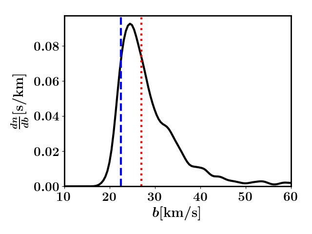
Figure 1: The line broadening probability distribution for lines with $0.8\leq\Delta\leq 1.2$, estimated by Kernel Density. We show the 10th and the 50th percentiles of the distribution as the dashed blue and dotted red lines, respectively.

In Figure 2, we compare the distribution of the line broadening in the plane $b$-$\Delta$ and in the plane $b$-$\tau_{0}$, to highlight their similarity, the absorbing lines are being binned in $\Delta$ (or $\tau_{0}$). The error bars on the 10th and 50th percentiles of the $b$-distribution are computed by bootstrapping the lines of sight, rather than the absorption lines themselves.

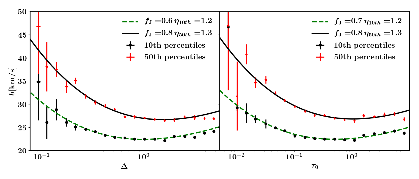
Figure 2: Percentiles of the line broadening, $b$, from 100 noiseless mock spectra versus the peak density contrast, $\Delta$ (left panel), and the peak neutral hydrogen optical depth, $\tau_{0}$ (right panel), in the redshift interval $2.9\leq z\leq 3.0$. The black dots (red stars) are the 10th (50th) percentiles of the $b$-distribution in the mock spectra. The error bars represent the 1-$\sigma$ uncertainty on the percentiles. In the left panel, the green dashed (solid black) line is a fit of our expression for the line broadening, Eq.( 13), to the 10th (50th) percentiles of the $b$-distribution divided in logarithmically and equally spaced intervals of $\Delta$. The values of $T_{0}$ and $\gamma$ are the result of the fit to the temperature-density relation, the values of $f_{\rm J}$ and $\eta$ are the result of the fit of the $b$-$\Delta$ relation. In the right panel, we have presented the analogous fit to the percentiles of the $b$-distribution as a function of $\tau_{0}$. In the transition from $b$-$\Delta$ space to $b$-$\tau_{0}$, the fitted values of $f_{\rm J}$ agree to within 15%. Our analytical expression for the line broadening correctly describes both the 10th and the 50th percentiles of line width distribution in our reference simulation, except for high values of $\tau_{0}$, where the downturn in $b$ is due to the onset of radiative cooling.

The minimum line broadening is a difficult quantity to measure. It is possible in noiseless spectra to measure an arbitrary percentile of the distribution of the line broadening, but that can only approximate the minimum line broadening. For this reason, we adapt Eq. (7), which we have written for the minimum line broadening, to the case of a generic percentile of the line broadening distribution, $b_{\rm perc}$

$$b_{\rm perc}^{2} = \eta_{\rm perc}^{2}(b_{T}^{2}+b_{\lambda}^{2})\,,$$ (13)

where $\eta_{\rm perc}$ is a constant that will depend on the chosen percentile of the $b$-distribution. This constant must be determined from simulations, an incorrect calibration will implies a systematic effect on the reconstruction of the IGM parameters. The impact of varying $\eta_{\rm perc}$ is discussed in B. Eq. (13) describes well both the 10th and the 50th percentiles of the absorption line broadening distribution up to $\tau_{0}\sim 10$. Nevertheless, the values of $f_{\rm J}$ can differ in the fits to the $b$-$\Delta$ distribution or to $b$-$\tau_{0}$ distribution. The discrepancy in $f_{\rm J}$ between these two distribution can be up to $\sim 15\%$. For $\tau_{0}\gtrapprox 10$ radiative cooling becomes relevant, although the precise value of $\tau_{0}$ for which this occurs depends on the specific values of $T_{0}$, $\gamma$, $\lambda_{\rm F}$ and $\Gamma_{\rm HI}$. In this work we only consider the case of power-law TDR, but we intend to address the problem of a general TDR in a future publication.

4 Method for reconstructing the absorption line broadening

In this section we will discuss how to reconstruct the minimum line broadening from spectra with noise, and then how to estimate $T$ and $\lambda_{\rm F}$. In the presence of noise and instrumental broadening, we cannot apply directly the formalism that we have developed in Garzilli et al. (2015b) for measuring the line broadening occurring in the Ly $\alpha$ forest to observed quasar spectra. In there the line broadening was estimated directly from the second derivative of the optical depth from mock spectra without noise, compare Eq.(18) of (Garzilli et al., 2015b). In spectra with noise, the computation of the second derivative in the measurement of $b$ is not stable under noise. In order to smooth out the noise, we first fit the sightlines with a superposition of Voigt profiles, and then apply the procedure we have already developed for noiseless sightlines on the spectra reconstructed from their Voigt profile decompositions, and determine $b$ and $\tau_{0}$ for each absorber. We then apply Eq. (13). In this section, we consider the case of mock sight lines to which we added noise with S/N=100. We use a sample size of a total 500 sightlines for each considered redshift interval, each spectrum has a length of $25\,c{\rm Mpc}$. If we analyze together all the signal coming from bins in redshift of $\Delta z=0.1$, then for redshifts ranging from $z=4$ to $2$, 500 sightlines correspond to a number of Lyman $\alpha$ quasar spectra varying from 180 to 85. This sample size is comparable with current sample size of observed high resolution and high signal to noise quasars, for example there are $\sim 500$ quasar spectra collected in Murphy et al. (2018).

4.1 Reconstructing the line broadening in the Ly$\alpha$ forest

We attempt to remove the noise in the mock sightlines, by fitting the Ly$\alpha$ stretch in the mock sightlines with noise with VPFIT (Carswell et al., 1987; Webb, 1987). The full spectrum flux is divided into intervals of variable length, between 10 and 15 Å. We start from the minimum wavelength in the Ly$\alpha$ stretch, $\lambda_{1}$, then we search for the maximum of the flux in the interval $[\lambda_{1}+10\,$Å$,\lambda_{1}+15\,$Å$]$, the wavelength corresponding to the maximum flux will be $\lambda_{2}$. Then, the maximum of the flux in the interval $[\lambda_{2}+10\,$Å$,\lambda_{2}+15\,$Å$]$ is identified and the corresponding wavelength will be $\lambda_{3}$. These maxima do not always coincide with the continuum, there is always some residual absorption. This process is repeated until the end of the spectrum has been reached. In this way the spectrum is subdivided into intervals of variable length. Each interval of transmitted flux is fit independently with VPFIT. The stopping criteria that we have considered is given by the change of the chi-square, $\Delta\chi^{2}$, between iteration steps. If $\chi^{2}<15$ then the iteration terminates if $\Delta\chi^{2}/\chi^{2}<5\times 10^{-4}$, otherwise if $\chi^{2}>15$ the iteration terminates if $\Delta\chi^{2}/\chi^{2}<5\times 10^{-3}$. The flux is also reconstructed separately for each independent stretch. We do not attempt to perform a full Voigt-profile fitting of the entire Ly$\alpha$ forest, because of the long computing time required for fitting automatically the entire Ly$\alpha$ forest in one batch. We are only interested in a noiseless reconstruction of the flux in the minimum $\chi^{2}$ sense. On the reconstructed optical depth we apply the ‘peak identification’ method and estimate the line broadening as described in Garzilli et al. (2015b) for the case of noiseless sightlines.

In Figure 3 we show a comparison between the 10th and 50th percentiles of the $b$-distribution for noiseless sightlines and for the reconstructed flux for the case of high and low S/N. We have considered 500 sightlines in the redshift interval $2.9\leq z\leq 3.0$. We would like to measure the minimum line broadening in the sightlines, hence ideally we would like to consider the 10th-percentiles of the line broadening. Nevertheless, we can see that qualitatively the 10th percentiles are not reconstructed very well in the sightlines with noise. Instead, the 50th percentiles (or medians) of the line broadening are reconstructed over a larger $\tau_{0}$ range. The reason is that noise increases the dispersion of the line broadening distribution at fixed $\Delta$. Hence, while the median of the distribution is not changed by this added dispersion, the 10th percentiles are changed. For this reason, in the following we will characterize the line broadening by considering the 50th percentiles of the $b$-distribution, rather than the 10th.

In Figures 4 we compare the PDF of the $b$-distribution as found in the noiseless sightlines and in the sightlines with noise, for two distinct intervals in $\tau_{0}$. For $0.08\leq\tau_{0}\leq 0.12$, the PDF of the reconstructed $b$ is much flatter then the PDF of the noiseless $b$, and the two PDFs do not match each other well. The number density of lines in the noiseless sightlines is $n_{\rm noiseless}=9.4\times 10^{-4}\,{\rm s\,km}^{-1}$, whereas the number of lines per length in the sightlines with noise is $n_{\rm noise}=8.4\times 10^{-4}\,{\rm s\,km^{-1}}$. For $0.8\leq\tau_{0}\leq 1.2$ the PDFs of the reconstructed and noiseless $b$ are quite similar, they both exhibit a sharp cut-off for low values of $b$ and a declining tail for large values of $b$. We conclude that the line broadening is reconstructed less accurately for smaller values of $\tau_{0}$. For $0.8\leq\tau_{0}\leq 1.2$, the number of lines per length in the noiseless sightlines is $n_{\rm noiseless}=7.1\times 10^{-4}\,{\rm s\,km}^{-1}$, whereas the number of lines per length in the sightlines with noise is $n_{\rm noise}=7.0\times 10^{-4}\,{\rm s\,km^{-1}}$. We note that the number density of reconstructed lines refers to both genuine absorption lines and to fictitious lines originating from noise. We can see that the number of reconstructed line is comparable to the number of genuine lines for both interval of the overdensity. This comparison allows us to say that we can determine the 50th percentiles of $b$ well for $\tau_{0}\sim 1$.

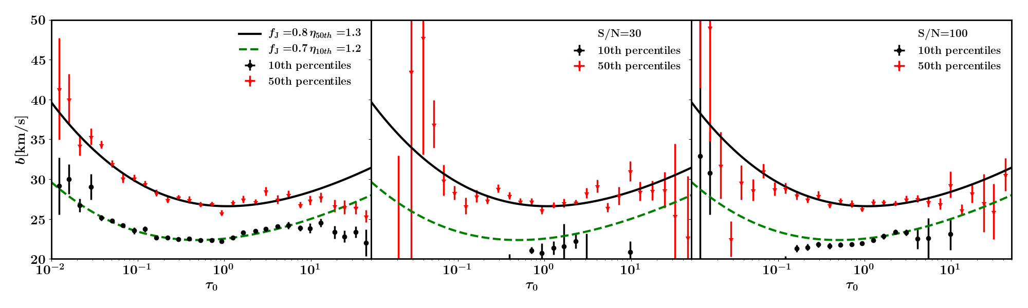
Figure 3: Comparison between the percentiles of the distribution of line broadening in the noiseless sightlines, and in the sightlines reconstructed with VPFIT, in the case of high and low signal-to-noise, for the redshift range $2.9\leq z\leq 3.0$. We have considered 500 lines of sight, each of length $25\,{\rm cMpc}$ . The left panels correspond to the noiseless case, the middle panel corresponds to the sightlines with noise with S/N=30, and the right panel to S/N=100. The black dots (red stars) are the 10th (50th) percentiles of the line broadening as a function of the central optical depth, $\tau_{0}$. The green dashed (black solid) line is the result of the fit of Eq.( 13) to the 10th (50th) percentiles of the $b$-distribution, where $T_{0}$ and $\gamma$ are inferred from the temperature-density relation, and $f_{\rm J}$ and $\eta$ are free parameters in the fit. In the case of reconstructed sightlines with VPFIT, the 10th percentiles of the $b$-distribution are very poorly reconstructed. In contrast, the 50th percentiles of the $b$-distribution are reconstructed well over a larger range of $\tau_{0}$. The robustness under reconstruction with VPFIT makes the 50th percentiles more suitable for the study of the properties of the IGM.

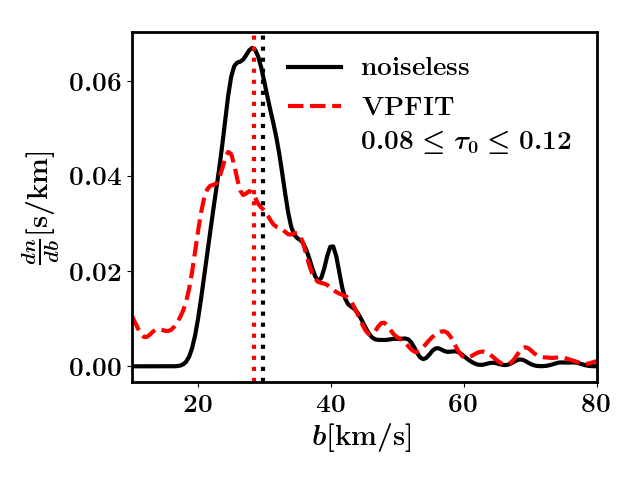
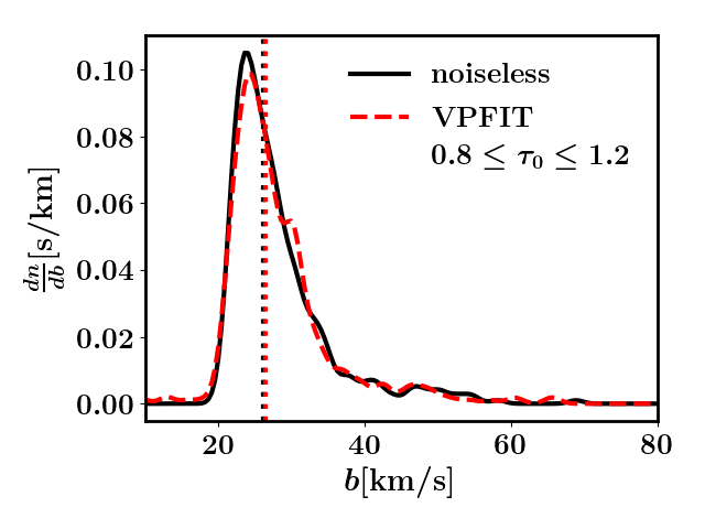
Figure 4: The probability density distribution of the logarithm of the line broadening, $\ln b$, for two values of the central optical depth, $\tau_{0}$, for 100 mock sightlines without noise and with noise (S/N=100). The probability density function has been estimated through kernel density estimate, with Gaussian kernel and the kernel bandwith is optimized by cross-validated grid-search over a grid. The left panel refers to the line broadening corresponding to $0.08\leq\tau_{0}\leq 0.12$, the right panel to $0.8\leq\tau_{0}\leq 1.2$. The black solid line is the PDF in the noiseless sightlines, the red dashed line is the one from the sightlines with noise. The black vertical line corresponds to the 50th percentile of the $b$-distribution in the noiseless sightlines, the red dashed vertical line corresponds to the 50th percentile of the $b$-distribution in the sightlines with noise. For the interval centered on $\tau_{0}\sim 0.1$, the number density of lines in the noiseless sightlines is $n_{\rm noiseless}=7.1\times 10^{−4}{\rm s/km}$, whereas the number of lines per length in the sightlines with noise is $n_{\rm noise}=7.0\times 10^{−4}{\rm s/km}$. For the interval centered on $\tau_{0}\sim 1$, the number density of lines in the noiseless sightlines is $n_{\rm noiseless}=9.4\times 10^{−4}{\rm s/km}$, whereas the number of lines per length in the sightlines with noise is $n_{\rm noise}=8.4\times 10^{−4}{\rm s/km}$.

4.2 Estimation of the IGM parameters

We have considered the estimation of the IGM parameters over a redshift interval $z\in[2.9,3.6]$, with a redshift step $\Delta z=0.1$.

We intend to estimate $T_{0}$, $\gamma$, $\lambda_{\rm F}$ and $\Gamma_{\rm HI}$. $T_{0}$ and $\gamma$ are the parameters of the TDR, and they have been the subject of many studies in the past, whereas the role of $\lambda_{\rm F}$ in setting the line broadening has been recognized only relatively recently, $\Gamma_{\rm HI}$ is a parameter that is usually kept fixed to a value. We have decided to vary $\Gamma_{\rm HI}$ because it affects the optical depth. In fact, when $\Gamma_{\rm HI}$ is inferred from observations, $T_{0}$ is assumed. As an example, we consider the cases of (Becker et al., 2011), (Becker & Bolton, 2013) and (Faucher-Giguère et al., 2008). In those work, $\Gamma_{\rm HI}$ is fixed to a value, the $T_{0}$ is measured. From the measurement of $T_{0}$, a new measurement of $\Gamma_{\rm HI}$ is inferred.

In order to get an estimate of all the parameters that are relevant for the IGM, we fit the measured 50th percentile of the $b$-distribution from the sightlines with noise with the model $b(\tau,T_{0},\gamma,\lambda_{\rm F},\Gamma_{\rm HI})$, our analytical formula for line broadening, Eq. (13). We have chosen the interval for the reconstructed central optical depth $\tau_{0}=[0.1,4]$, in order to exclude the region affected by cooling and by noise. We divide the central optical depth into equi-spaced logarithmic intervals, and we compute the median of the line broadening for each central optical depth bin. We indicate the resulting collection of central optical depth and median line broadening values with ${\hat{\tau_{i}},\hat{b}_{i}}$, where $i$ is index that varies on the bins of the central optical depth. We also estimate the 1-$\sigma$ error on $\hat{b_{i}}$, $\sigma(\hat{b}_{i})$. The errors are estimated by bootstrapping the lines of sight, rather than the absorption lines. The theoretical model is indicated with the notation $b_{i}(T_{0},\gamma,\lambda_{\rm F},\Gamma_{\rm HI})=b(\tau_{i},T_{0},\gamma,\lambda_{\rm F},\Gamma_{\rm HI})$. The constant $\eta_{50th}$, appearing in Eq. (13), has been calibrated using our reference simulation, separately for each redshift interval, as in Table 1. In Appendix B, we have explicitly tested the effect of changing $\eta_{50th}$ by $\pm 5\%$, and we have demonstrated that our results are unchanged.

Table 1: Values of $\eta_{50th}$, appearing in Eq. (13), calibrated from the noiseless mock spectra from our reference simulation as a function of redshift, $z$.

$z$	$\eta_{50th}$
2.95	1.32
3.05	1.27
3.15	1.25
3.25	1.28
3.34	1.26
3.45	1.26
3.56	1.25

In order to perform the fit, we compute the chi-squared function, $\chi^{2}$, defined as

$$\chi^{2} = \sum_{i}\left(b_{i}(T_{0},\gamma,\lambda_{\rm F},\Gamma_{\rm HI})-\hat{b_{i}}\right)^{2}/\sigma(\hat{b_{i}})^{2}\,,$$ (14)

where $b(T_{0},\gamma,\lambda_{\rm J},\Gamma_{\rm HI})$ is the line broadening as computed from Eq. (13), $\hat{b}$ is the 50th percentile of $b$-distribution. We compute the corresponding likelihood function by ${\cal L}=\exp(-\chi^{2}/2)$ and maximize the likelihood by using Montepython (Audren et al., 2013), CosmoMC (Lewis & Bridle, 2002) and Polychord (Handley et al., 2015a, b). We have chosen logarithmic priors on $T_{0}$, $\Gamma_{\rm HI}$ and $\lambda_{\rm F}$ and a flat prior on $\gamma$, which are summarized in Table 2.

Table 2: Prior ranges considered for the parameter of the maximum likelihood analysis, used for fitting the mock median line broadening data to the model given by Eq. (13). We have chosen logarithmic priors on $T_{0}$, $\Gamma_{\rm HI}$ and $\lambda_{\rm F}$ and a linear prior on $\gamma$. Here and in the rest of the paper, $\log$ indicates the logarithm in base 10.

	min	max
$\log(T_{0}[{\rm K}])$	0	5
$\gamma$	1	2
$\log(\lambda_{\rm F}[{\rm cMpc}]$)	-3	3
$\log(\Gamma_{\rm HI}[{\rm s^{-1}}])$	-13	-11

Before presenting the joint fit of all parameters, we show in Figure 5 how the minimal line broadening is affected by each parameter independently, using our analytical model of the line broadening in Eq. (13). Changing $T_{0}$ is almost equivalent to changing the line broadening by a multiplicative factor. Changing $\lambda_{\rm F}$ mostly affects the line broadening at small $\tau_{0}$. Changing $\gamma$ affects the slope of the line broadening at all $\tau_{0}$. Changing $\Gamma_{\rm HI}$ has the effect of changing the neutral fraction of hydrogen, hence it affects the $\Delta$-$\tau_{0}$ relation, and it shifts the position in the minimum of the $b$-$\tau_{0}$ relation. The effect of $\Gamma_{\rm HI}$ is only to shift the curves of line broadening left to right, but not up and down. We can expect some degeneracies between the estimated parameters in the final analysis: $\gamma$ and $\Gamma_{\rm HI}$ appear to be correlated, $T_{0}$ and $\gamma$ appear to be anti-correlated, $T_{0}$ and $\lambda_{\rm F}$ anti-correlated, $\lambda_{\rm F}$ and $\Gamma_{\rm HI}$ correlated.

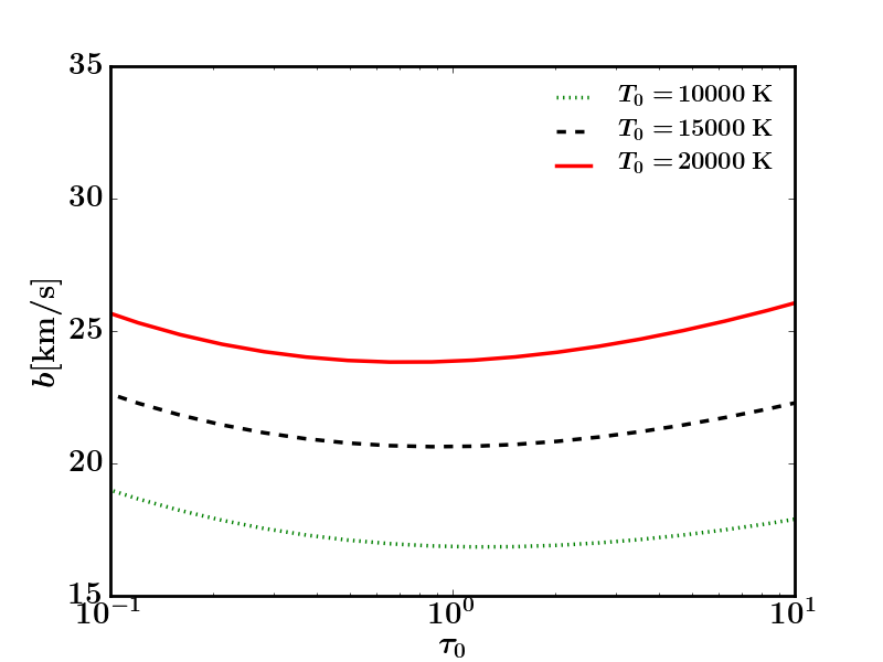
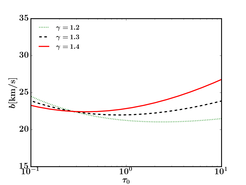
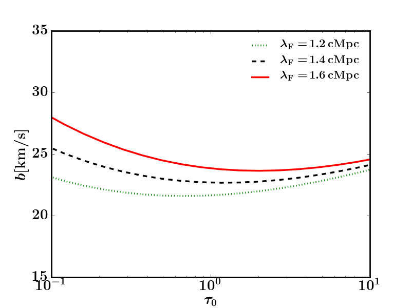
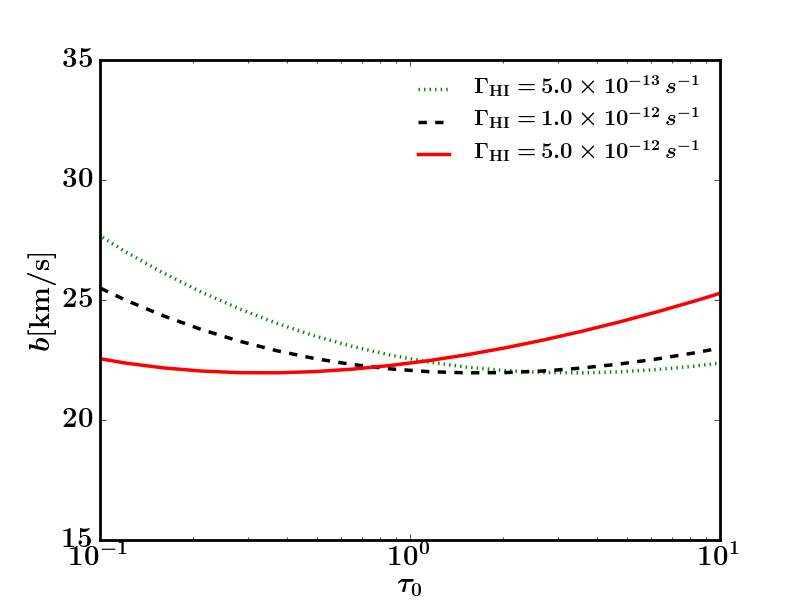
Figure 5: The effect on the line broadening of varying $T_{0}$, $\gamma$, $\lambda_{\rm F}$ and $\Gamma_{\rm HI}$ independently. The line broadening is computed from Eq. (13) for $z=3.0$ (with $\eta=1$). The parameters that are not shown in the label are fixed to $T_{0}=17000\,{\rm K}$, $\lambda_{\rm F}=1.4\,{\rm cMpc}$, $\gamma=1.3$, $\Gamma_{\rm HI}=10^{-12}\,{\rm s^{-1}}$.

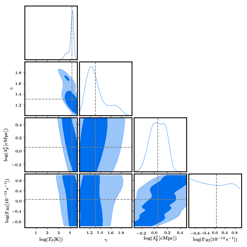
Figure 6: The likelihood contours for the analysis of the median line broadening distribution at $z=3.05$. The likelihood exploration has been done with Montepython (Audren et al., 2013) and the result plotted with GetDist utility in CosmoMC. The likelihood contours that we have shown in the panels refers to 68% and 95% confidence level. The measured value of $T_{0}$ is anti-correlated with both $\gamma$ and $\lambda_{\rm F}$. The value of $\Gamma_{\rm HI}$ is correlated with $\lambda_{\rm F}$. The origin of these degeneracies can be understood by comparing to Figure 5. The true values in the simulations are represented by the horizontal and vertical dashed lines.

In Figure 6, we show the likelihood contours for the parameters estimated for the redshift interval $3.0\leq z\leq 3.1$. The number of data points is 12 and the number of free parameters is 4, hence the number of degree of freedom is 8. The expected anti-correlations in $\lambda_{\rm F}$-$T_{0}$ and $\gamma$-$T_{0}$ are visible, and also the correlation between $\Gamma_{\rm HI}$ and $\lambda_{\rm F}$. In order to improve the constraining power of our method, resolve the degeneracies between the parameters, and mitigate the effect of the assumed priors on $\Gamma_{\rm HI}$ and $\lambda_{\rm F}$, we combine the fit to the distribution of the line broadening with the fit of the median of the flux. We consider the analytical description of the optical depth that we have given in Equation 11, we can verify that it correctly describes the median optical depth at the peak as a function of the density contrast. We attempt to use this relation to describe the median flux, by applying $F=\exp(-\tau)$, and considering the distribution of density contrast as found in our reference simulation. When we consider the median of the flux (on all the spectra and not only on the peaks of the optical depth), we find that Equation 11 does not match the results found in mock spectra. This was expected, because Equation 11 describes the relation between the optical depth at the peak of the line and the underlying density contrast.

In order to account for this unknown factor, in the comparison with the mean optical depth, we will consider the $T_{0}$ intervening in 11 as an additional nuisance parameter, that we will call $\omega$. The $\chi^{2}$ for the joint analysis of the line broadening and median flux will be the sum of the $\chi^{2}$ in Eq. 14 and

$$\chi^{2} = \sum_{i}\Big{(}M_{\Delta}(\exp(-\tau(\Delta,\omega,\gamma,\lambda_{\rm F},\Gamma_{\rm HI}))$$

$$- M(F)\Big{)}^{2}/\sigma(M(F))^{2}\,,$$

where $\tau(\Delta,\omega,\gamma,\lambda_{\rm F},\Gamma_{\rm HI})$ is the relation between $\tau_{0}$ and $\Delta$ in Eq. 11 (with the nuisance parameter $\omega$ instead of $T_{0}$ ), $M_{\Delta}(y(\Delta))$ represents taking the median of the function $y$ by varying $\Delta$ over all the values of the density contrast in the simulation, $M(F)$ is the median of $F$ as found in the mock spectra, and $\sigma(M(F))$ is the error on the median flux in mock spectra and it is computed by bootstrap. In the future application of this method to observed spectra, we will consider the distribution of density contrast as found in our reference simulation. We let the nuisance parameter $\omega$ free to vary in the interval $[0,5]$. Now the number of data points is 13, the number of free parameters is 5, hence the number of degree of freedom is 8. In Figure 7, we show the likelihood contours for the parameters estimated for the redshift interval $3.0\leq z\leq 3.1$. There is an anti-correlation between $T_{0}$ and $\lambda_{\rm F}$, between $\gamma$ and $T_{0}$, and between $\Gamma_{\rm HI}$ and $\omega$, whereas $\gamma$ and $\lambda_{\rm F}$ are correlated. We show the results of this joint analysis between the line broadening distribution and the median flux in Figure 8. The parameters $T_{0}$,$\gamma$ and $\lambda_{\rm F}$ are detected at 2-$\sigma$ level in all the considered redshift bins, and in excellent agreement with the true values measured from the simulation, whereas there exist lower limits for $\Gamma_{\rm HI}$ at 2-$\sigma$ level.

Here, we note that the comoving size of the filaments at cosmic mean density is $\sim 1\,{\rm cMpc}$ in all the examined redshift intervals. This value exceeds by an order of magnitude the estimate of the filtering length given in (Rorai et al., 2017). Indeed, Rorai et al. use N-body simulations for modeling the distribution of dark matter, then they impose a smoothing filter, with a single filtering length, for describing the baryonic density. As discussed in Schaye et al. (2000b), and as we have explicitly shown in Figure 3 of Garzilli et al. (2015b), the physical size of the absorbers is not a single value, but it is a power-law relation of the density. Because Rorai et al. does not explicitly quantify to which density range they are more sensitive, it is not possible to make a direct comparison with their work.

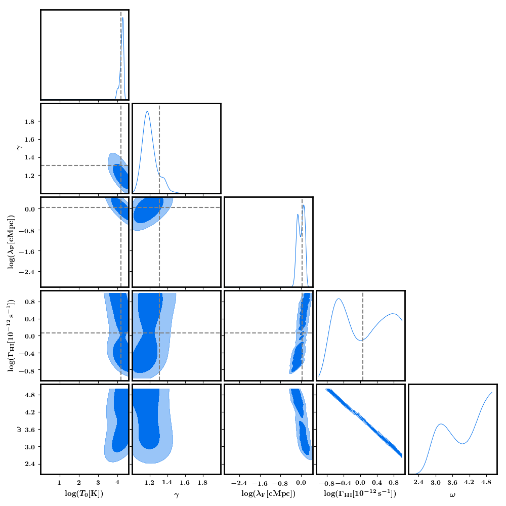
Figure 7: The likelihood contours for the joint analysis of the median line broadening distribution and the median flux at $z=3.05$, same conventions as in Figure 6. There is a slight anti-correlation between $T_{0}$ and $\lambda_{\rm F}$, a slight correlation between $\lambda_{\rm F}$ and $\Gamma_{\rm HI}$, and an evident correlation between $\Gamma_{\rm HI}$ and $\omega$. The estimated parameters ranges are in excellent agreement with their true values ($\omega$ is a nuisance parameters and it does not have an associated true value).

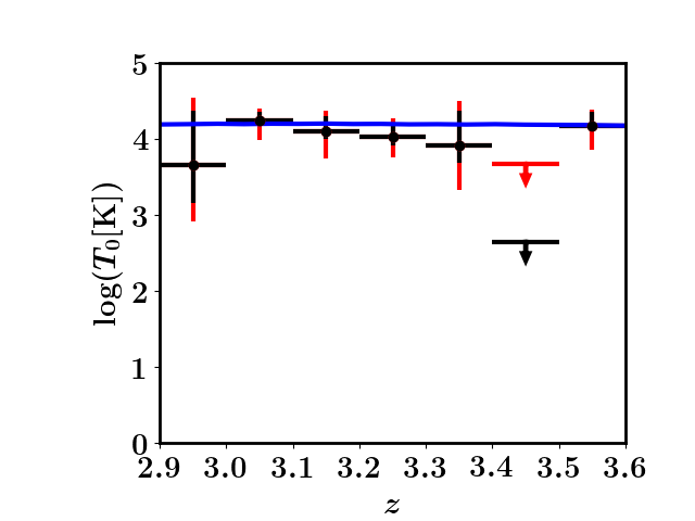
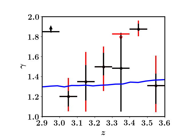
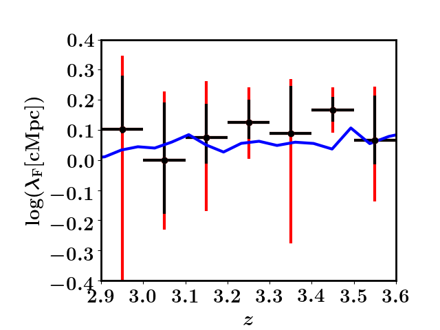
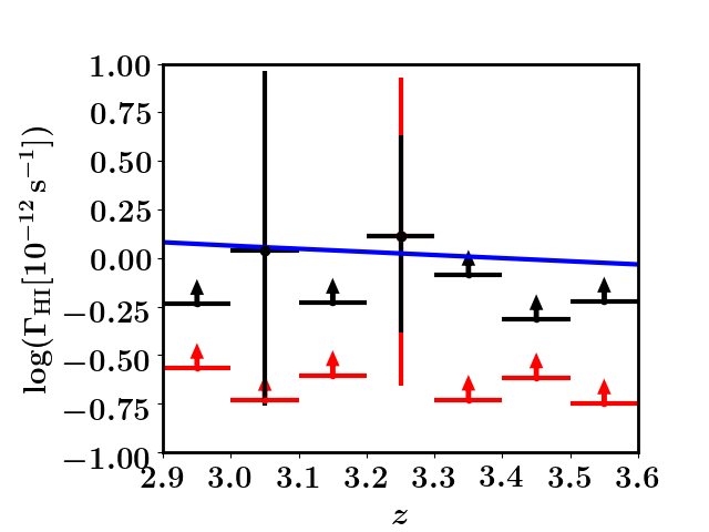
Figure 8: The result of estimation of $T_{0}$, $\gamma$, $\lambda_{\rm F}^{0}$ and $\Gamma_{\rm HI}$ for the analysis as in Figure 7 for all the redshift intervals . The black error bars indicate the 1-$\sigma$ errors, and the red error bars are the 2-$\sigma$ contours. The numbers on the top of each panel show the reduced chi-squared, $\hat{\chi^{2}}=\chi^{2}/n_{\rm dof}$, where $n_{\rm dof}$ is the number of degrees of freedom, that in this analysis is 13-5=8 for each redshift interval. The solid blue line are the values of the parameters measured from the simulations. All the parameters are constrained in all the redshift bins.

5 Conclusions

We have described a new method to measure the IGM temperature and the widths of the filaments that are responsible for the absorption in the Ly$\alpha$ forest, based on the description of the minimum line broadening that we have developed in Garzilli et al. (2015b) and on the description of the median flux that we have described here. In the original formulation, we derived a relation between the minimum line broadening of the Ly$\alpha$ forest and the over-density, $\Delta$. Because $\Delta$ is a quantity that cannot be measured directly in observed quasar spectra, we reformulated the minimum line broadening description in terms of the central line optical depth, $\tau_{0}$, that can be measured directly.

In this work we considered the problem of reconstructing the line broadening in spectra with noise and finite instrumental resolution. We used automatic Voigt profile decompositions by VPFIT to reconstruct noiseless spectra from noisy data, and to this reconstructed spectra we applied the method for finding the lines and computing the line broadening for noiseless sightlines that we described in Garzilli et al. (2015b). We have found that the 10th percentiles of the line broadening are not very well reconstructed for the smallest values of $\tau_{0}$, whereas the median line broadening is more robust.

We applied our method to a sample of mock sightlines extracted from our reference simulation with low and high signal to noise. Our method is calibrated to our reference numerical simulation in two ways. Concerning the line broadening distribution, we have determined the multiplying factor needed to match the median line broadening to the minimal line broadening from the reference simulation. Concerning the median flux, we consider the density contrast taken from our reference simulation, and we use it to compute the observable median flux. We combine the analysis of the line broadening distribution with the analysis of the median flux. We are going to discuss in an upcoming work the application of our method to observational data. In fact, our method allows us to reconstruct the properties of the IGM, such as the temperature, the size of the expanding filaments at the cosmic mean density, and, partially, the photo-ionisation rate of neutral hydrogen.

We aim to apply this method to observed quasar spectra, in order to obtain new measurements of the IGM temperature and of the sizes of the absorbing structures. These measurements will be presented in a forthcoming paper.

Appendix A A comparison with traditional Voigt profile fitting

We consider the reconstruction of percentiles of line broadening obtained from Voigt profile fitting, which has been widely used in the literature. Voigt profile fitting has been considered in Schaye et al. (1999, 2000a); Ricotti et al. (2000); McDonald et al. (2001); Bolton et al. (2012); Rudie et al. (2012) for measuring the IGM temperature, and it is the only line decomposition technique applied so far to the Ly$\alpha$ forest, using a variety of codes like VPFIT, FITLYMAN (Fontana & Ballester, 1995) or AUTOVP (Dave et al., 1997). Voigt profile fitting is a global fitting method that implies fitting the entire shape of the transmitted flux. Hence, it is sensitive to the clustering of the absorbers in the Ly$\alpha$ forest, in other words, it is sensitive to the underlying density distribution of the gas. In fact, some Voigt profiles with very small $b_{\rm VPFIT}$ are present, because they improve the overall convergence of the fit. Instead, our ‘peak decomposition’ only measures the line broadening at “local maxima” in the optical depth. We have applied Voigt profile fitting to our mock sightlines with noise using VPFIT (Carswell et al., 1987; Webb, 1987). In Figure 9 we show the resulting $b_{\rm VPFIT}$-$N_{\rm HI}$ distribution, and compare it with the amount of line broadening described by Eq.( 13). The upturn of the $b$-$N_{\rm HI}$ distribution that is expected for small $N_{\rm HI}$ is visible neither in the 10th nor 50th percentiles of the $b_{\rm VPFIT}$ distribution.

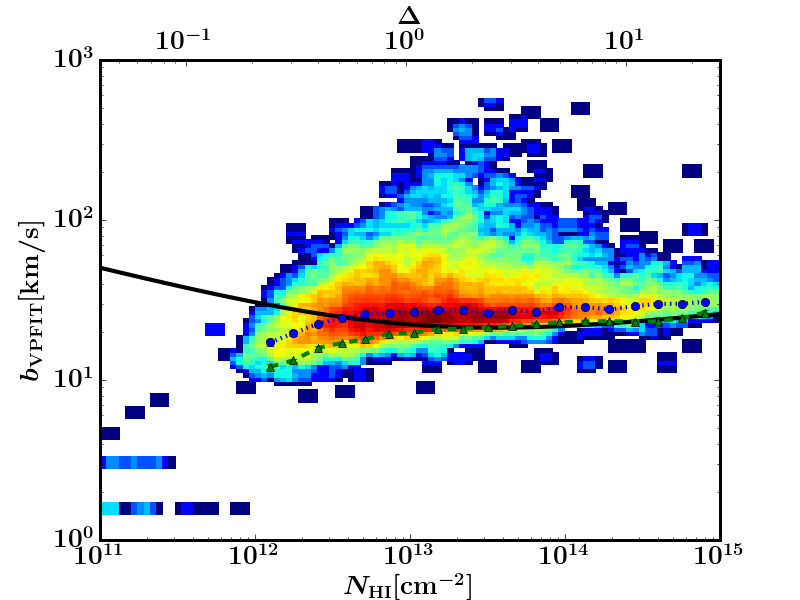
Figure 9: The distribution of line broadening as obtained from VPFIT, $b_{\rm VPFIT}$, versus the neutral hydrogen column density, $N_{\rm HI}$. The color scheme encodes the number density of the lines in the $b_{\rm VPFIT}$-$N_{\rm HI}$ plane. The blue dots (green triangles) connected by a dotted (dashed) line are the 50th (10th) percentiles of the $b_{\rm VPFIT}$-distribution in equally spaced logarithmic intervals of $N_{\rm HI}$. The solid black line is the line of minimum line broadening, from Eq. (25) Garzilli et al. (2015b). Both the 10th and the 50th percentiles of the $b_{\rm VPFIT}$-distribution turn towards low values of $b_{\rm VPFIT}$ for low values of $N_{\rm HI}$, these percentiles look different from the case of $b$ measured with our method, shown in Figure 3, where the percentiles of the $b$ distribution turn towards high values of $b$ for low values of $\tau_{0}$, as expected theoretically.

Appendix B Effect of the uncertainty on $\eta_{50}$

We show that changing the values of $\eta_{50}$ by $\div 5\%$ does not affect the result of our analysis. In Figure 10 (Figure 11) we show the constraints on the IGM parameters for the case that $\eta_{50}$ is increased (decreased) by $5\%$. We infer that a variation of $\eta_{50}$ within $5\%$ does not affect the result of our analysis.

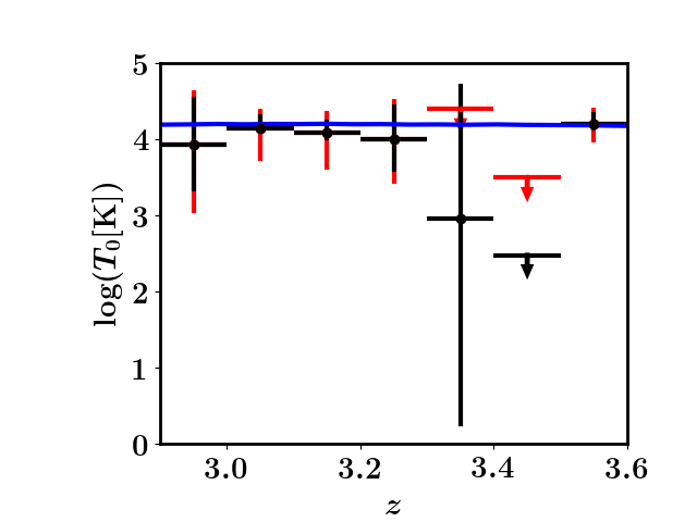
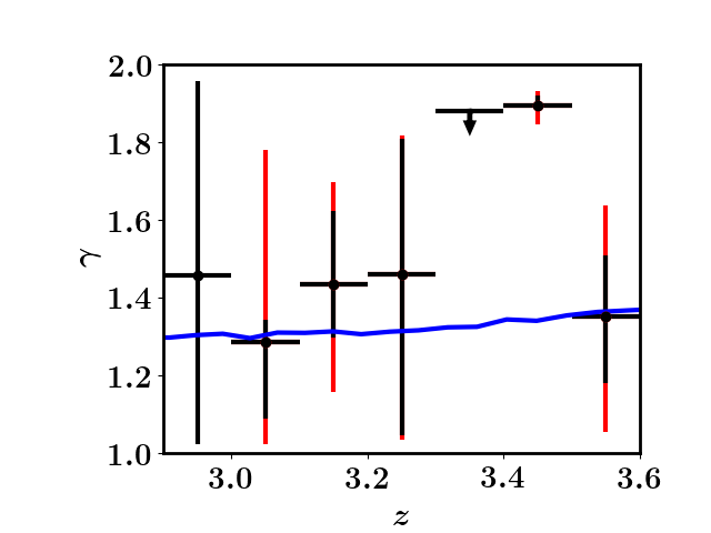
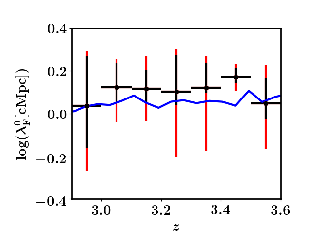
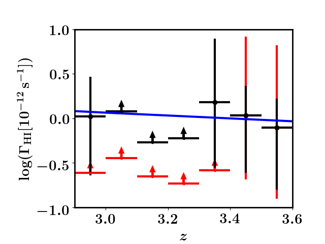
Figure 10: The results of $T_{0}$, $\gamma$, $\lambda_{\rm F}$ and $\Gamma_{\rm HI}$ estimation for a value of $\eta_{50}$ increased by $5\%$ respect to the value calibrated from our reference simulation. The analysis is performed as in Fig. 8, and we apply the same conventions. The result of this analysis show that our method is robust respect to calibration for an increase of $\eta_{50}$ of $5\%$.

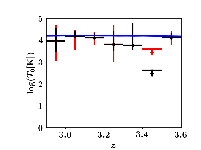
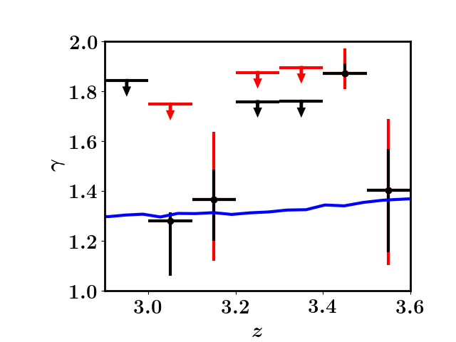
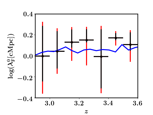
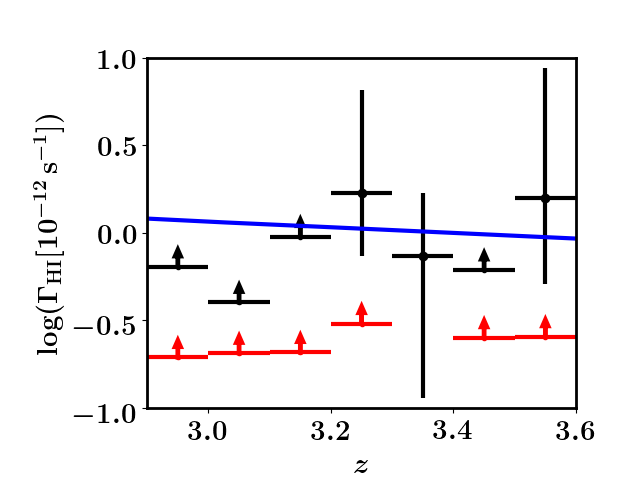
Figure 11: The results of $T_{0}$, $\gamma$, $\lambda_{\rm F}$ and $\Gamma_{\rm HI}$ estimation for a value of $\eta_{50}$ decreased by $5\%$ respect to the value calibrated from our reference simulation. The analysis is performed as in Fig. 8, and we apply the same conventions. The result of this analysis show that our method is robust respect to calibration for an decrease of $\eta_{50}$ of $5\%$.

Appendix C Considering lower S/N

In Figure 12 we show the results of the parameters estimation for the case of a low signal-to-noise sample of spectra (S/N=30) for the central optical depth interval $\tau_{0}\in[0.3,4]$ (that is different from the optical depth interval that we have chosen for the high signal-to-noise sample). The results are similar to the ones found in the high signal-to-noise case, but with larger error bars.

We conclude that our method also works with lower signal to noise spectra, and it is hence applicable to existing spectra.

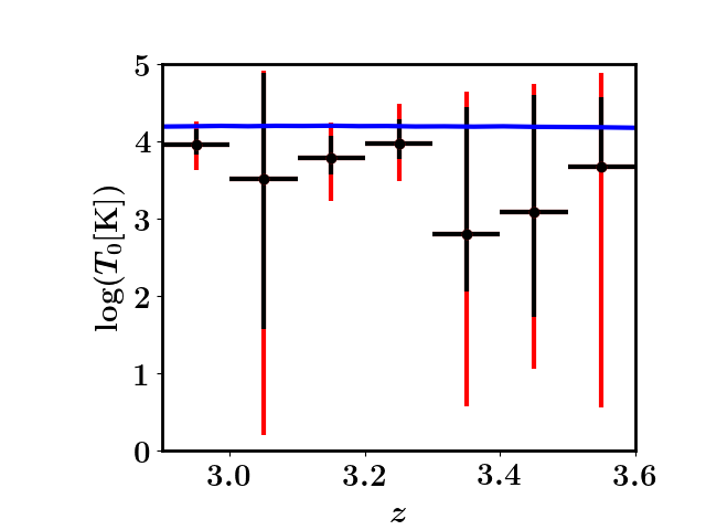
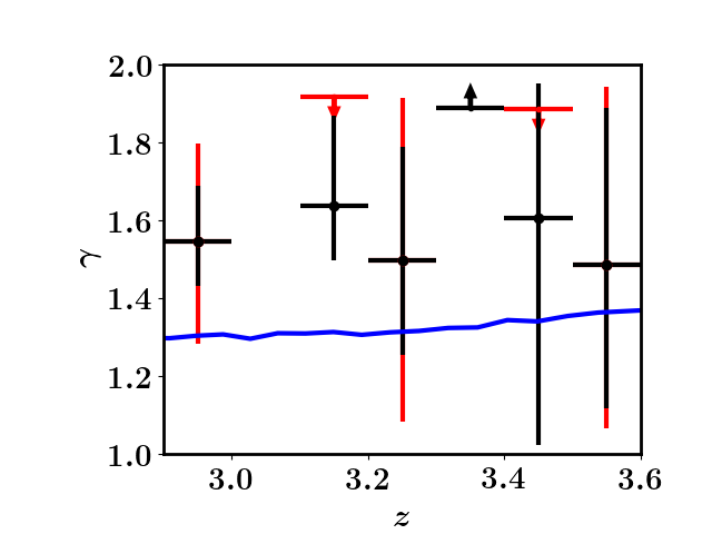
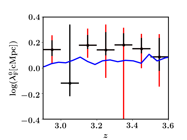
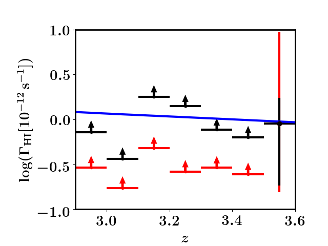
Figure 12: The results of $T_{0}$, $\gamma$, $\lambda_{\rm F}$ and $\Gamma_{\rm HI}$ estimation for the case of lower signal-to-noise spectra (S/N=30), each redshift bin is analyzed independently. The $b$-$\tau_{0}$ relation is fitted in the interval $\tau_{0}\in[0.3,4]$. There are no constraints on $\Gamma_{\rm HI}$. Same conventions as in Fig. 8.

References

- Altay & Theuns (2013) Altay G., Theuns T., 2013, MNRAS, 434, 748
- Audren et al. (2013) Audren B., Lesgourgues J., Benabed K., Prunet S., 2013, JCAP, 1302, 001
- Becker & Bolton (2013) Becker G. D., Bolton J. S., 2013, Mon. Not. Roy. Astron. Soc., 436, 1023
- Becker et al. (2011) Becker G. D., Bolton J. S., Haehnelt M. G., Sargent W. L. W., 2011, MNRAS, 410, 1096
- Bolton et al. (2005) Bolton J. S., Haehnelt M. G., Viel M., Springel V., 2005, MNRAS, 357, 1178
- Bolton et al. (2008) Bolton J. S., Viel M., Kim T.-S., Haehnelt M. G., Carswell R. F., 2008, MNRAS, 386, 1131
- Bolton et al. (2012) Bolton J. S., Becker G. D., Raskutti S., Wyithe J. S. B., Haehnelt M. G., Sargent W. L. W., 2012, MNRAS, 419, 2880
- Bolton et al. (2014) Bolton J. S., Becker G. D., Haehnelt M. G., Viel M., 2014, MNRAS, 438, 2499
- Calura et al. (2012) Calura F., Tescari E., D’Odorico V., Viel M., Cristiani S., Kim T.-S., Bolton J. S., 2012, MNRAS, 422, 3019
- Cantalupo et al. (2014) Cantalupo S., Arrigoni-Battaia F., Prochaska J. X., Hennawi J. F., Madau P., 2014, Nature, 506, 63
- Carswell et al. (1987) Carswell R. F., Webb J. K., Baldwin J. A., Atwood B., 1987, ApJ, 319, 709
- Crain et al. (2015) Crain R. A., et al., 2015, MNRAS, 450, 1937
- Dave et al. (1997) Dave R., Hernquist L., Weinberg D. H., Katz N., 1997, Astrophys. J., 477, 21
- Desjacques & Nusser (2005) Desjacques V., Nusser A., 2005, Mon. Not. Roy. Astron. Soc., 361, 1257
- Faucher-Giguère et al. (2008) Faucher-Giguère C.-A., Lidz A., Hernquist L., Zaldarriaga M., 2008, ApJ, 688, 85
- Fontana & Ballester (1995) Fontana A., Ballester P., 1995, The Messenger, 80, 37
- Fumagalli et al. (2017) Fumagalli M., Haardt F., Theuns T., Morris S. L., Cantalupo S., Madau P., Fossati M., 2017, MNRAS, 467, 4802
- Gaikwad et al. (2017) Gaikwad P., Srianand R., Choudhury T. R., Khaire V., 2017, Mon. Not. Roy. Astron. Soc., 467, 3172
- Gaikwad et al. (2018a) Gaikwad P., Srianand R., Khaire V., Choudhury T. R., 2018a
- Gaikwad et al. (2018b) Gaikwad P., Choudhury T. R., Srianand R., Khaire V., 2018b, Mon. Not. Roy. Astron. Soc., 474, 2233
- Garzilli et al. (2012) Garzilli A., Bolton J. S., Kim T.-S., Leach S., Viel M., 2012, MNRAS, 424, 1723
- Garzilli et al. (2015a) Garzilli A., Theuns T., Schaye J., 2015a, MNRAS, 450, 1465
- Garzilli et al. (2015b) Garzilli A., Theuns T., Schaye J., 2015b, Mon. Not. Roy. Astron. Soc., 450, 1465
- Garzilli et al. (2017) Garzilli A., Boyarsky A., Ruchayskiy O., 2017, Phys. Lett., B773, 258
- Garzilli et al. (2018) Garzilli A., Magalich A., Theuns T., Frenk C. S., Weniger C., Ruchayskiy O., Boyarsky A., 2018, ] 10.1093/mnras/stz2188
- Gnedin & Hui (1998) Gnedin N. Y., Hui L., 1998, MNRAS, 296, 44
- Gunn & Peterson (1965) Gunn J. E., Peterson B. A., 1965, ApJ, 142, 1633
- Haardt & Madau (1996) Haardt F., Madau P., 1996, ApJ, 461, 20
- Haardt & Madau (2001) Haardt F., Madau P., 2001, in Neumann D. M., Tran J. T. V., eds, Clusters of Galaxies and the High Redshift Universe Observed in X-rays. (arXiv:astro-ph/0106018)
- Handley et al. (2015a) Handley W. J., Hobson M. P., Lasenby A. N., 2015a, Mon. Not. Roy. Astron. Soc., 450, L61
- Handley et al. (2015b) Handley W. J., Hobson M. P., Lasenby A. N., 2015b, Monthly Notices of the Royal Astronomical Society, 453, 4385–4399
- Hiss et al. (2017) Hiss H., Walther M., Hennawi J. F., Oñorbe J., O’Meara J. M., Rorai A., 2017, preprint, (arXiv:1710.00700)
- Hui & Gnedin (1997) Hui L., Gnedin N. Y., 1997, MNRAS, 292, 27
- Hui et al. (1997) Hui L., Gnedin N. Y., Zhang Y., 1997, ApJ, 486, 599
- Khaire et al. (2019) Khaire V., et al., 2019, Mon. Not. Roy. Astron. Soc., 486, 769
- Kim et al. (2007) Kim T.-S., Bolton J. S., Viel M., Haehnelt M. G., Carswell R. F., 2007, MNRAS, 382, 1657
- Kirkman et al. (2005) Kirkman D., et al., 2005, MNRAS, 360, 1373
- Kulkarni et al. (2015) Kulkarni G., Hennawi J. F., Oñorbe J., Rorai A., Springel V., 2015, Astrophys. J., 812, 30
- Lewis & Bridle (2002) Lewis A., Bridle S., 2002, Phys. Rev., D66, 103511
- Lidz et al. (2010) Lidz A., Faucher-Giguère C.-A., Dall’Aglio A., McQuinn M., Fechner C., Zaldarriaga M., Hernquist L., Dutta S., 2010, ApJ, 718, 199
- Madau & Haardt (2015) Madau P., Haardt F., 2015, Astrophys. J., 813, L8
- McAlpine et al. (2016) McAlpine S., et al., 2016, Astronomy and Computing, 15, 72
- McDonald & Miralda-Escudé (2001) McDonald P., Miralda-Escudé J., 2001, ApJ, 549, L11
- McDonald et al. (2001) McDonald P., Miralda-Escudé J., Rauch M., Sargent W. L. W., Barlow T. A., Cen R., 2001, ApJ, 562, 52
- McQuinn et al. (2009) McQuinn M., Lidz A., Zaldarriaga M., Hernquist L., Hopkins P. F., Dutta S., Faucher-Giguère C.-A., 2009, ApJ, 694, 842
- Meiksin (2009) Meiksin A. A., 2009, Reviews of Modern Physics, 81, 1405
- Meiksin & White (2004) Meiksin A., White M., 2004, MNRAS, 350, 1107
- Menzel & Pekeris (1935) Menzel D. H., Pekeris C. L., 1935, MNRAS, 96, 77
- Miralda-Escude & Rees (1993) Miralda-Escude J., Rees M. J., 1993, MNRAS, 260, 617
- Murphy et al. (2018) Murphy M. T., Kacprzak G. G., Savorgnan G. A. D., Carswell R. F., 2018, MNRAS,
- Peeples et al. (2010) Peeples M. S., Weinberg D. H., Dave R., Fardal M. A., Katz N., 2010, Mon. Not. Roy. Astron. Soc., 404, 1281
- Planck Collaboration et al. (2014) Planck Collaboration et al., 2014, A&A, 571, A16
- Puchwein et al. (2015) Puchwein E., Bolton J. S., Haehnelt M. G., Madau P., Becker G. D., Haardt F., 2015, Mon. Not. Roy. Astron. Soc., 450, 4081
- Puchwein et al. (2019) Puchwein E., Haardt F., Haehnelt M. G., Madau P., 2019, Mon. Not. Roy. Astron. Soc., 485, 47
- Rauch (1998) Rauch M., 1998, ARA&A, 36, 267
- Rauch et al. (1997) Rauch M., et al., 1997, ApJ, 489, 7
- Ricotti et al. (2000) Ricotti M., Gnedin N. Y., Shull J. M., 2000, ApJ, 534, 41
- Rorai et al. (2013) Rorai A., Hennawi J. F., White M., 2013, ApJ, 775, 81
- Rorai et al. (2017) Rorai A., et al., 2017, preprint, (arXiv:1704.08366)
- Rudie et al. (2012) Rudie G. C., Steidel C. C., Pettini M., 2012, ApJ, 757, L30
- Sanderbeck et al. (2016) Sanderbeck P. R. U., D’Aloisio A., McQuinn M. J., 2016, Mon. Not. Roy. Astron. Soc., 460, 1885
- Schaller et al. (2015) Schaller M., Dalla Vecchia C., Schaye J., Bower R. G., Theuns T., Crain R. A., Furlong M., McCarthy I. G., 2015, MNRAS, 454, 2277
- Schaye (2001) Schaye J., 2001, ApJ, 559, 507
- Schaye et al. (1999) Schaye J., Theuns T., Leonard A., Efstathiou G., 1999, MNRAS, 310, 57
- Schaye et al. (2000a) Schaye J., Theuns T., Rauch M., Efstathiou G., Sargent W. L. W., 2000a, Mon. Not. Roy. Astron. Soc., 318, 817
- Schaye et al. (2000b) Schaye J., Theuns T., Rauch M., Efstathiou G., Sargent W. L. W., 2000b, MNRAS, 318, 817
- Schaye et al. (2015) Schaye J., Crain R. A., Bower R. G., etcetera 2015, MNRAS, 446, 521
- Seljak et al. (2006) Seljak U., Makarov A., McDonald P., Trac H., 2006, Phys. Rev. Lett., 97, 191303
- Springel (2005) Springel V., 2005, MNRAS, 364, 1105
- Theuns & Zaroubi (2000) Theuns T., Zaroubi S., 2000, MNRAS, 317, 989
- Theuns et al. (1998a) Theuns T., Leonard A., Efstathiou G., Pearce F. R., Thomas P. A., 1998a, MNRAS, 301, 478
- Theuns et al. (1998b) Theuns T., Leonard A., Efstathiou G., Pearce F. R., Thomas P. A., 1998b, MNRAS, 301, 478
- Theuns et al. (2000) Theuns T., Schaye J., Haehnelt M. G., 2000, MNRAS, 315, 600
- Viel & Haehnelt (2006) Viel M., Haehnelt M. G., 2006, Mon. Not. Roy. Astron. Soc., 365, 231
- Viel et al. (2009) Viel M., Bolton J. S., Haehnelt M. G., 2009, MNRAS, 399, L39
- Viel et al. (2013) Viel M., Schaye J., Booth C. M., 2013, MNRAS, 429, 1734
- Viel et al. (2017) Viel M., Haehnelt M. G., Bolton J. S., Kim T. S., Puchwein E., Nasir F., Wakker B. P., 2017, Mon. Not. Roy. Astron. Soc., 467, L86
- Vogt et al. (1994) Vogt S. S., et al., 1994, in Crawford D. L., Craine E. R., eds, Proc. SPIEVol. 2198, Instrumentation in Astronomy VIII. p. 362, doi:10.1117/12.176725
- Webb (1987) Webb J. K., 1987, PhD thesis, PhD thesis, Univ. Cambridge, 1987.
- Wiersma et al. (2009a) Wiersma R. P. C., Schaye J., Smith B. D., 2009a, MNRAS, 393, 99
- Wiersma et al. (2009b) Wiersma R. P. C., Schaye J., Theuns T., Dalla Vecchia C., Tornatore L., 2009b, MNRAS, 399, 574
- Zaldarriaga et al. (2001) Zaldarriaga M., Hui L., Tegmark M., 2001, ApJ, 557, 519