Percolation on Isotropically Directed Lattice

Abstract

We investigate percolation on a randomly directed lattice, an intermediate between standard percolation and directed percolation, focusing on the isotropic case in which bonds on opposite directions occur with the same probability. We derive exact results for the percolation threshold on planar lattices, and present a conjecture for the value the percolation-threshold for in any lattice. We also identify presumably universal critical exponents, including a fractal dimension, associated with the strongly-connected components both for planar and cubic lattices. These critical exponents are different from those associated either with standard percolation or with directed percolation.

I Introduction

In a seminal paper published some 60 years ago, Broadbent and Hammersley (Broadbent and Hammersley, 1957) introduced the percolation model, in a very general fashion, as consisting of a number of sites interconnected by one or two directed bonds which could transmit information in opposite directions. However, over the years, most of the attention has been focused on the limiting cases of standard percolation, in which bonds in both directions are either present or absent simultaneously, and of directed percolation, in which only bonds in a preferred direction are allowed. While standard percolation represents one of the simplest models for investigating critical phenomena in equilibrium statistical physics (Stauffer and Aharony, 1994), directed percolation has become a paradigmatic model for investigating non equilibrium phase transitions (Marro and Dickman, 2005). Moreover, it has been shown that the isotropic case, where bonds in both opposite directions are present with the same probability is a very particular case, with any amount of anisotropy driving the system into the same universality class as that of directed percolation (Hans-Karl Janssen and Olaf Stenull, 2000; Hu et al., 2014; Redner, 1982a).

The case of percolation on isotropically directed lattices has received much less attention. This modified percolation model should be particularly relevant to the understanding of a large number of physical systems. For instance, in the same way that standard percolation was shown to be related to other models in statistical mechanics (Fortuin and Kasteleyn, 1972) one could expect percolation on isotropically directed lattices to be related to statistical systems with non-symmetric interactions (Lima, 2010). It has been shown that identifying the connected components systems with non-symmetric interactions can elucidate questions regarding the controllability (Liu and Barabási, 2016) and observability (Santolini and Barabási, 2018) of these systems. Percolation with directed bonds have also been investigated in the field of traffic dynamics (Li et al., 2015).Redner (Redner, 1981, 1982a, 1982b) formulated the problem of percolation on isotropically directed lattices as a random insulator-resistor-diode circuit model, in which single directed bonds represent diodes, allowing current to flow in only one direction, while double bonds in opposite directions represent resistors and absent bonds represent insulators.

Focusing on hypercubic lattices, he employed an approximate real-space renormalization-group treatment which produces fixed points associated with both standard percolation (in which only resistors and insulators are allowed) and directed percolation (in which only insulators and diodes conducting in a single allowed direction are present), as well as other “mixed” fixed points controlling lines of critical points, for cases in which the all three types of circuit elements are present. The crossover from isotropic to directed percolation when there is a slight preference for one direction was studied via computer simulations (Inui et al., 1999) and renormalized field theory (Hans-Karl Janssen and Olaf Stenull, 2000; Stenull and Janssen, 2001). More recently, the same crossover problem was independently investigated on the square and on the simple-cubic lattices by Zhou et al. (Zhou et al., 2012), who dubbed their model “biased directed percolation”.

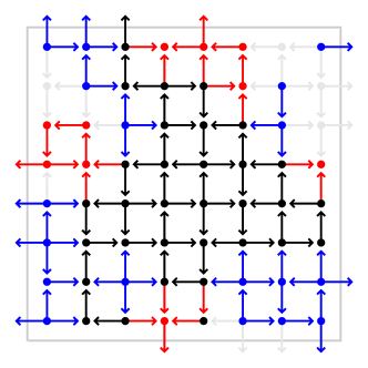
Figure 1: A square lattice where each pair of nearest neighbors is connected by a directed bond at the critical point  Zhou et al. (2012). The color code is as follows: Black indicates nodes and bonds comprising the largest strongly connected component (GSCC), that is, the largest set of nodes that can be mutally reached from each other. Red indicates nodes and bonds outside the GSCC that can be reached from nodes in the GSCC. Blue indicates nodes and bonds outside the GSCC from where nodes in the GSCC can be reached. The largest outgoing/incoming component (GOUT/GIN) includes all nodes of the GSCC augmented by the red/blue nodes, respectively. Grey indicates nodes and bonds outside both GIN and GOUT. Bonds exiting the enclosing box represent connections through the periodic boundary condition.

We are interested here in percolation of isotropically directed bonds in which bonds in opposite directions are present with the same probability, possibly along with vacancies and undirected bonds. It has been conjectured that this model is in the same universality class as standard percolation Hans-Karl Janssen and Olaf Stenull (2000); Zhou et al. (2012), however these works have focused on the sets of nodes that can be reached from a given point. In fact, when considering directed bonds, it is possible that site A can be reached from site B, while site B cannot be reached from site A, what therefore calls for a redefinition of a cluster. Percolation of directed bonds was investigated within the context of complex networks (Dorogovtsev et al., 2001; Schwartz et al., 2002; Boguñá and Serrano, 2005; Kenah and Robins, 2007; Ángeles Serrano and De Los Rios, 2007; Franceschet, 2012; Zhu et al., 2014; Li et al., 2015), where the concept of strongly-connected components (SCCs) has been adopted (Tarjan, 1972), defined as those sets of points which can be mutually reached following strictly the bond directions. A critical state of the model can be characterized as the point where a giant strongly connected component (GSCC) is formed (Dorogovtsev et al., 2001). Alternatively, one can define a giant cluster formed by all the sites that can be reached from a given site following bond directions (GOUT) (Dorogovtsev et al., 2001), and determine the critical point where such cluster is formed. Alternatively, one can define a giant cluster formed by all the sites that can be reached from a given site following bond directions (Dorogovtsev et al., 2001), and determine the critical point where such cluster is formed. There is no logical need for these two points to be the same, leaving the possibility of two distinct phase transitions existing in this model (Schwartz et al., 2002). However, both for regular lattices, as we will show here, and for some complex networks (Dorogovtsev et al., 2001), these two objects form at the same critical point. In Fig. 1 we show an example of a square lattice at the critical point.

This paper is organized as follows. In Section II we define the model and present calculations of percolation thresholds. In Section III we discuss some exact results on hierarchical lattice that shed light on the critical state of this model. Our computer simulation results are presented in Section IV, while Section V is dedicated to a concluding discussion.

II Definition of the model and calculation of percolation thresholds

We work on $d$-dimensional regular lattices. All sites are assumed to be present, but there are a few possibilities for the connectivity between nearest-neighbors. With probability $p_{0}$ they may not be connected (indicating a vacancy). With probability $p_{1}$ they may be connected by a directed bond (with equal probabilities for either direction). Finally, with probability $p_{2}$ neighbors may be connected by an undirected bond (or equivalently by two having opposite directions). Of course we must fulfill $p_{0}+p_{1}+p_{2}=1$.

A simple heuristic argument yields an expression for the critical threshold for percolation of isotropically directed bonds. Starting from a given site $i$ on a very large lattice, the probability $p_{nn}$ that a particular nearest-neighbor site can be reached from $i$ is given by the probability that both directed bonds are present between these neighbors ($p_{2}$) plus the probability that there is only one directed bond and that it is oriented in the appropriate direction ($\frac{1}{2}p_{1}$). As the distribution of orientations is on average isotropic, the critical threshold must depend only on $p_{nn}$. In fact, using the Leath-Alexandrowicz method  (Leath, 1976; Alexandrowicz, 1980), it can be shown (Zhou et al., 2012) that the clusters of sites reached from a seed site in percolation of directed bonds with a given $p_{nn}$ are identically distributed to the clusters of standard percolation with an occupation $p_{sp}$, as long as $p_{sp}=p_{nn}$. Therefore, we conclude that the critical percolation probabilities of our model should fulfill

$$p_{2}+\tfrac{1}{2}p_{1}=p_{c},$$ (1)

in which $p_{c}$ is the bond-percolation threshold for standard percolation in the lattice.

We can use duality arguments to show that Eq. (1) is indeed exact for the square, triangular and honeycomb lattices. A duality transformation for percolation of directed bonds on planar lattices was previously introduced (Redner, 1982a) to derive the percolation threshold on the square lattice. The transformation states that every time a directed bond is present in the original lattice, the directed bond in the dual lattice that crosses the original bond forming an angle of $\frac{\pi}{2}$ clockwise will be absent. With the opposite also holding, namely every time a directed bond is absent in the original lattice, in the dual lattice the bond forming a angle $\frac{\pi}{2}$ clockwise will be present. Of course, an undirected bond (or alternatively two bonds in opposite directions) in the original lattice corresponds to a vacancy in the dual lattice, and vice-versa. Figure 2(a) shows a configuration of percolation of directed bonds on the triangular lattice and the corresponding dual honeycomb lattice.

Denoting by $q_{0}$, $q_{1}$ and $q_{2}$ the respective probabilities that there is a vacancy, a single directed bond, or an undirected bond between nearest neighbors on the dual lattice, the transformation allows us to write,

$$q_{0}=p_{2},\quad q_{1}=p_{1},\quad q_{2}=p_{0}.$$ (2)

From these results and the normalization conditions

$$p_{0}+p_{1}+p_{2}=q_{0}+q_{1}+q_{2}=1$$ (3)

we immediately obtain

$$\tfrac{1}{2}\left(p_{2}+q_{2}\right)+\tfrac{1}{2}p_{1}=\tfrac{1}{2},$$

which is valid for any choice of the probabilities. As already noticed by Redner (Redner, 1982a), for the square lattice, which is its own dual, we must have $p_{2}=q_{2}$ at the percolation threshold, yielding

$$p_{2}+\tfrac{1}{2}p_{1}=\tfrac{1}{2},$$ (4)

in agreement with Eq. (1). Here, of course, we assume that there is only one critical point.

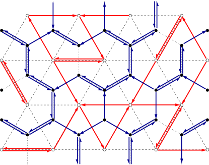
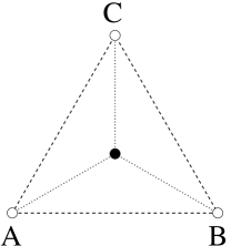
Figure 2: (a) Illustration of a configuration of percolation of directed bonds on the triangular (white sites, red arrows) and honeycomb (black sites, blue arrows) lattices, related by the dual transformation defined in the text. (b) The sites involved in the star-triangle transformation discussed in the text.

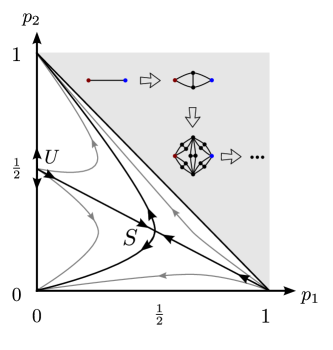
Figure 3: Phase diagram for percolation of isotropically directed bonds on the hierarchical lattice obtained as the limit of the process displayed. Redner (Redner, 1981, 1982a) and Dorogovtsev (Dorogovtsev, 1982) used the renormalization group to solve exactly this model on the shown hierarchical lattice. The directions of the lines indicate the renormalization group flux. The critical line $p_{2}+p_{1}/2=1/2$ coincides with the critical line for percolation of isotropically directed bonds on the square lattice. The renormalization group shows that any point on the critical line, besides $U=(0,1/2)$ that corresponds to the critical point of standard percolation, will display the same scale invariant behavior as a point $S$ located along the critical line, suggesting the possibility that percolation of isotropically directed bonds may be in a different universality class from standard percolation.

The triangular and the honeycomb lattices are related by the duality transformation, as illustrated in Fig. 2(a), and we now use a star-triangle transformation (Sykes and Essam, 1964) to calculate their bond-percolation thresholds. Based on enumerating the configurations of bonds connecting the sites identified in Fig. 2(b), we can calculate the probabilities $P$ and $Q$ of connections between the sites on the star and on the triangle, respectively. For the probability that site A is connected only to site B or only to site C, we obtain

$$P_{\text{AB}}=\tfrac{1}{2}p_{1}p_{2}^{2}+\tfrac{1}{2}p_{1}^{2}p_{2}+\tfrac{1}{8}p_{1}^{3}+p_{0}p_{2}^{2}+p_{0}p_{1}p_{2}+\tfrac{1}{4}p_{0}p_{1}^{2},$$

$$Q_{\text{AB}}=\tfrac{1}{4}q_{1}^{2}q_{2}+\tfrac{1}{8}q_{1}^{3}+q_{0}q_{1}q_{2}+\tfrac{1}{2}q_{0}q_{1}^{2}+q_{0}^{2}q_{2}+\tfrac{1}{2}q_{0}^{2}q_{1},$$

with $P_{\text{AC}}=P_{\text{AB}}$ and $Q_{\text{AC}}=Q_{\text{AB}}$. For the probability that site A is connected to both sites B and C, we have

$$P_{\text{ABC}}=p_{2}^{3}+\tfrac{3}{2}p_{1}p_{2}^{2}+\tfrac{3}{4}p_{1}^{2}p_{2}+\tfrac{1}{8}p_{1}^{3},$$

$$Q_{\text{ABC}}=q_{2}^{3}+3q_{1}q_{2}^{2}+\tfrac{9}{4}q_{1}^{2}q_{2}+\tfrac{1}{2}q_{1}^{3}+3q_{0}q_{2}^{2}+3q_{0}q_{1}q_{2}+\tfrac{3}{4}q_{0}q_{1}^{2}.$$

At the percolation threshold, we must have $P_{\text{AB}}=Q_{\text{AB}}$ and $P_{\text{ABC}}=Q_{\text{ABC}}$, and taking into account the normalization conditions in Eq. (3) we obtain

$$p_{2}+\tfrac{1}{2}p_{1}=1-2\sin\tfrac{\pi}{18}=p_{c}^{(\text{honeycomb)}}$$ (5)

and

$$q_{2}+\tfrac{1}{2}q_{1}=2\sin\tfrac{\pi}{18}=p_{c}^{(\text{triangular})},$$ (6)

again in agreement with Eq. (1).

All these predictions show that at least one of the critical percolation points of isotropically directed bonds, when a giant out-going component (GOUT) is formed, can be simply related to the model of standard percolation by Eq. (1). Our numerical results indicate that the critical point defined by the formation of a GSCC coincides with the formation of a GOUT. However, as we show in the following section, compared to the GOUT, the GSCC has a different set of critical exponents.

III Critical state of the percolation of isotropically directed bonds

Redner (Redner, 1981, 1982a) and Dorogovtsev (Dorogovtsev, 1982) solved exactly percolation of directed bonds on a hierarchical lattice obtained by iterating the process shown in Fig. 3. Having the probabilities $p_{0}$, $p_{1}$, and $p_{2}$ at a given generation of the process, renormalization group calculations allow one to determine the probabilities $p^{\prime}_{0}$, $p^{\prime}_{1}$, and $p^{\prime}_{2}$, of the next generation. The scale invariant states are the fixed points of the renormalization group. As shown in Fig. 3, two of those points represent the trivial cases of a fully disconnected lattice $p_{0}=1$ and a fully connected lattice $p_{2}=1$. Another fixed point is $p_{1}=0$ with $p_{2}=1/2$ representing the critical scale invariant state for standard percolation in this hierarchical lattice, while the remaining one, $p_{1}=0.49142$ with $p_{2}=0.25429$, is the critical scale invariant state for percolation of isotropically directed bonds in this hierarchical lattice. Surprisingly, this hierarchical lattice has similarities with the square lattice (Redner, 1981, 1982a), as it can predict exactly, not only the critical point of standard percolation, but also the whole critical line $p_{2}+p_{1}/2=1/2$. With the exception of the critical state of standard percolation, all the other points along the critical line converge through the renormalization process towards the scale invariant state of percolation of isotropically directed bonds.

Although these renormalization group calculations do not yield precise predictions for the correlation-length exponent $\nu$ in $2D$, they give the same value $\nu=\ln_{2}(13/8)\approx 1.428$ for both standard percolation as well as percolation of isotropically directed bonds (Redner, 1981, 1982a). Moreover, there are two order-parameter exponents $\beta_{1}=0.1342$ and $\beta_{2}=0.1550$ that are related to clusters which percolate in a single direction or in both directions, respectively (Redner, 1981, 1982a). Again here the method does not obtain exactly the value of the exponent $\beta$ for $2D$, presented in the next Section, but shows that $\beta_{1}$ is the same value as the one obtained for standard percolation in this hierarchical lattice, while $\beta_{2}$ is shown to be a different exponent. These two different exponents indicate, at least for this hierarchical lattice, that percolation on isotropically directed bonds is tricritical.

In the next Section, we show that simulation results for the square, honeycomb and triangular lattices confirm Eqs. (4)–(6). Furthermore, we show that indeed the fractal dimensions of the two forms of critical giant clusters, GSCC and GOUT, are different from each other, but seemingly universal among the different lattices.

IV Simulation results

We start by describing our results for two dimensions, while the $3D$ case will be discussed subsequently. We simulated bidimensional lattices with linear size ranging from $L=32$ to $L=8192$, taking averages over a number of samples ranging from $38400$ (for $L=32$) to $150$ (for $L=8192$), halving the number of samples each time that the linear size was doubled. Periodic boundary conditions were employed.

Besides checking the predictions for the percolation threshold, our goal is to obtain the values of the critical exponents associated with (i) clusters which can be traversed in one direction and (ii) clusters which can be traversed in both directions. In the language of complex networks, these clusters correspond in case (i) to giant out-components (GOUT) and in case (ii) to the giant strongly-connected component (GSCC). For each sample, we identified all the SCCs by using Tarjan’s algorithm (Tarjan, 1972), and calculated their size distribution. At the percolation threshold, we also looked at the giant outgoing component (GOUT), which corresponds to the GSCC augmented by sites outside of it which can be reached from those in the GSCC. By symmetry, the statistical properties of the GOUT must be the same as those of the giant in-component (GIN), defined as the set of sites not in the GSCC from which we can reach the GSCC, augmented by sites in the GSCC itself. Figure 1 shows an example of a square lattice with $L=16$, indicating the GSCC, the GOUT, and the GIN. Some of the results presented next were obtained with the help of the Graph Tool software library (Peixoto, 2014).

We define the order parameter here as the fraction of sites belonging to the largest SCC. For an infinite planar lattice, this order parameter should behave as

$$\lim_{L\rightarrow\infty}\frac{\left\langle S\right\rangle}{L^{2}}\sim\left(p-p_{c}\right)^{\beta_{scc}},$$ (7)

where $\left\langle S\right\rangle$ is the average size of the largest SCC, $p$ is a parameter that controls the distance to the critical point $p_{c}$, and $\beta_{scc}$ is expected to be a universal critical exponent. A finite-size scaling ansatz for the order parameter is

$$\frac{\left\langle S\right\rangle}{L^{2}}\sim L^{-\beta_{scc}/\nu}f_{1}\left(\left(p-p_{c}\right)L^{1/\nu}\right),$$ (8)

in which $\nu$ is the correlation-length critical exponent and $f_{1}\left(x\right)$ is a scaling function. From this ansatz, we see that precisely at the critical point we should have

$$\frac{\left\langle S\right\rangle}{L^{2}}\sim L^{-\beta_{scc}/\nu}.$$ (9)

Similarly, we can look at the second moment of the SCC size distribution (excluding the GSCC), which, for an infinite lattice, should behave as

$$\lim_{L\rightarrow\infty}\left\langle S^{2}\right\rangle\sim\left(p-p_{c}\right)^{-\gamma_{scc}},$$ (10)

with $\gamma_{scc}$ being another universal critical exponent. The corresponding finite-size scaling ansatz is

$$\left\langle S^{2}\right\rangle\sim L^{\gamma_{scc}/\nu}f_{2}\left(\left(p-p_{c}\right)L^{1/\nu}\right),$$ (11)

where $f_{2}\left(x\right)$ is also a scaling function, and precisely at the critical point we should have

$$\left\langle S^{2}\right\rangle\sim L^{\gamma_{scc}/\nu}.$$ (12)

In order to obtain values for these critical exponents, we have to introduce a parameterization of the probabilities $p_{0}$, $p_{1}$ and $p_{2}$. We performed two different sets of simulations, with different parameterizations. In the first set of numerical experiments, bonds were occupied with probabilities parameterized as

$$p_{0}=\left(1-p\right)^{2},\quad p_{1}=2p\left(1-p\right),\quad p_{2}=p^{2},$$ (13)

with $0\leq p\leq 1$, so that, according to Eq. (1), we have $p=p_{c}$ at the percolation threshold. This corresponds to randomly assigning on directed bond with probability $p$ on each possible direction of each pair of nearest neighbors; two opposite directed bonds between the same pair correspond to an undirected bond.

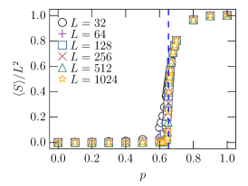
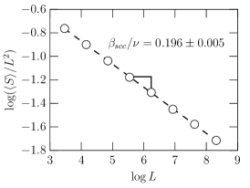
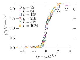
Figure 4: These results correspond to a honeycomb lattice where each possible directed bond is occupied with probability $p$, with opposite bonds between the same pair of sites being present with probability $p^{2}$, as parameterized in Eq. (13). a) The order parameter for percolation of isotropically directed bonds defined as the fraction of nodes in the largest strongly connected component (GSCC). b) At the critical point the fraction occupied by the GSCC decays as a power law, yielding the exponent $\beta_{scc}/\nu$. c) Using the value obtained for $\beta_{scc}/\nu$, and assuming that the exponent $\nu$ for percolation of isotropically directed bonds is the same as in standard percolation, $\nu=4/3$, we can collapse all the curves near the critical point. Here, and in all other plots, error bars are smaller than the symbols.

Figure 4 shows results for the SCC order parameter for honeycomb lattices with sizes ranging from $L=32$ to $1024$. As depicted in Fig. 4(a), the threshold probability is consistent with the result $p\simeq 0.653$ predicted by Eq. (5). Figure 4(b) plots the SCC order parameter at the critical point, which is expected to scale as in Eq. (9), a scaling form from which we extract $\beta_{scc}/\nu=0.196\pm 0.005$. Finally, Fig. 4(c) shows a rescaling of the finite-size results according to Eq. (8). It is a well known fact (Stauffer, 1994) that percolation has a single length scale given by the correlation length $\xi$ that diverges at the critical point as $\xi\sim N^{-\nu}$. Since there is no reason to expect that percolation on isotropically directed lattices introduces other length scales it is reasonable to assume that the exponent $\nu$ controlling the scale divergence of SCCs near the critical point is the same as in traditional percolation. This conjecture is supported by the renormalization group predictions of Redner (Redner, 1981) and of Janssen and Stenull Hans-Karl Janssen and Olaf Stenull (2000); Zhou et al. (2012) for the square lattice. Therefore, the best data collapse is obtained assuming for the correlation-length critical exponent the same value as in standard percolation, $\nu=\frac{4}{3}$, which leads to

$$\beta_{scc}=0.264\pm 0.008.$$

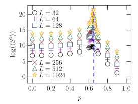
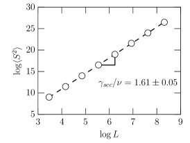
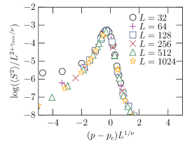
Figure 5: These results correspond to a honeycomb lattice where each possible directed bond is occupied with probability $p$, with opposite bonds between the same pair of sites being present with probability $p^{2}$, as parameterized in Eq. (13). a) The second moment of the distribution of sizes of SCCs, excluding the largest SCC. b) At the critical point the second moment grows as a power law, yielding the exponent $\gamma_{scc}/\nu$. c) Using the value obtained for $\gamma_{scc}/\nu$, and assuming $\nu=4/3$, we can collapse all the curves near the critical point.

For the second moment of the SCC size distribution, Fig. 5 shows results for honeycomb lattices. As shown in Fig. 5(a), the value of the percolation threshold is compatible with the prediction of Eq. (5), while from Fig. 5(b) and Eq. (12) we obtain $\gamma_{scc}/\nu=1.61\pm 0.05$. Again, the best data collapse of Eq. (11), shown in Fig. 5(c), is obtained by using $\nu=\frac{4}{3}$, yielding

$$\gamma_{scc}=2.15\pm 0.07.$$

Lattice	$\beta_{scc}$	$\mathrm{\gamma}_{scc}$	$d_{scc}$
Triangular	$\,0.264(8)\,$	$\,2.15(7)\,$	$\,1.804(5)\,$
Square	$\,0.261(5)\,$	$\,2.13(3)\,$	$\,1.801(8)\,$
Hexagonal	$\,0.27(1)\,$	$\,2.15(7)\,$	$\,1.80(1)\,$

Table 1: Values of the critical exponents related to the SCCs, as obtained for the triangular, square and hexagonal lattices, for the cases where each possible directed bond is occupied with probability $p$, with opposite bonds between the same pair of sites being present with probability $p^{2}$, as parameterized in Eq. (13). Numbers in parentheses indicate the estimated error in the last digit.

Table 1 summarizes the critical exponents obtained under the first parameterization for the triangular, square, and honeycomb lattices. We mention that the values obtained for $\beta_{scc}$ and $\gamma_{scc}$ are all compatible with values extracted from the simulation results by fitting the data for the largest linear size with the scaling predictions in Eqs. (7) and (10). We also measured the mass of the GSCC, denoted by $M_{scc}$, which is predicted to follow

$$M_{scc}\sim L^{d_{scc}},$$

with a fractal dimension

$$d_{scc}=2-\beta_{scc}/\nu.$$

This is confirmed by the measurements of $d_{scc}$ reported in the last column of Table 1.

In the second set of simulations, bonds were occupied with probabilities

$$p_{0}= \max\left(0,1-2p\right),\quad p_{1}=2\min\left(p,1-p\right),$$ (14)

$$p_{2}=\max\left(0,2p-1\right),$$

again with $0\leq p\leq 1$. These probabilities mean that for $p\leq\tfrac{1}{2}$ there are no undirected bonds, while for $p\geq\tfrac{1}{2}$ there are no vacancies. Exactly at $p=\frac{1}{2}$ there is a randomly directed bond between each pair of nearest neighbors. Again, according to Eq. (1), we have $p=p_{c}$ at the percolation threshold. The results for the GSCC properties measured under this second parameterization are compatible with those obtained under the first parameterization. As shown in Table 2, the critical exponents $\beta_{scc}$ and $\gamma_{scc}$ and the fractal dimension $d_{scc}$ are all compatible with the values obtained under the first parameterization.

Lattice	$\beta_{scc}$	$\mathrm{\gamma}_{scc}$	$d_{scc}$	$\tau_{scc}$
Triangular	$\,0.26(1)\,$	$\,2.16(8)\,$	$\,1.805(8)\,$	$\,2.07(9)\,$
Square	$\,0.26(1)\,$	$\,2.17(4)\,$	$\,1.802(8)\,$	$\,2.11(8)\,$
Hexagonal	$\,0.27(1)\,$	$\,2.16(7)\,$	$\,1.80(1)\,$	$\,2.12(8)\,$

Table 2: Values of the critical exponents related to the SCCs, as obtained for the triangular, square and hexagonal lattices for the case where undirected bonds appear only when all possible vacancies have already been occupied by a directed bond, as parameterized by Eq.(14). Numbers in parentheses again indicate the estimated error in the last digit. Within the error bars these values are compatible with those of Table 1.

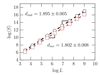
Figure 6: The fractal dimensions for the GSCC (squares) and the GOUT (circles). These results concern square lattices where all nearest neighbors are connected by a directed bond. This corresponds to the critical condition when using the parametrization given by Eq.(14). While the fractal dimension of GOUT is compatible with that of standard percolation clusters, the GSCCs have a smaller fractal dimension.

Under the second parameterization, besides measuring the mass of the GSCC associated with the fractal dimension $d_{scc}$, we also measured the mass of the GOUT, denoted by $M_{out}$, which scales as

$$M_{out}\sim L^{d_{out}},$$

where $d_{out}$ is a fractal dimension. We expect $d_{scc}\leq d_{out}$, as the GSCC is a subset of the GOUT. Indeed, as shown in Fig. 6, for the square lattice at the critical point, the fractal dimension $d_{out}$ of the GOUT is compatible with the exact fractal dimension $d_{f}=91/48$ (Stauffer, 1994) of the critical percolating cluster in standard percolation, while the value for $d_{scc}$ is about 10% smaller.

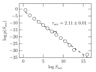
Figure 7: Scaling behavior of the SCC size distribution $p\left(S\right)$ for a square lattice with $L=8196$, under the second parameterization.

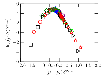
Figure 8: Scaling behavior of the SCC size distribution $p\left(S\right)$ for a square lattice with $L=4096$, under the second parametrization. The results are for $p=p_{c}+\delta$ with $\delta=-0.01$ (black squares), $\delta=-0.005$ (red circles), $\delta=-0.0025$ (green diamonds), $\delta=-0.00075$ (blue cross), $\delta=0.00075$ (violet x), $\delta=0.0025$ (lime up triangles), $\delta=0.005$ (black right triangles) and $\delta=0.01$ (red stars).

Finally, we looked at the exponents $\tau_{scc}$ and $\sigma_{scc}$ associated with the SCC size distribution, expected to scale as

$$p\left(S\right)\sim S^{-\tau_{scc}}f_{3}\left(\left(p-p_{c}\right)S^{\sigma_{scc}}\right),$$ (15)

where $f_{3}\left(x\right)$ is yet another scaling function. The Fisher exponent $\tau_{scc}$ associated with the scaling behavior of the SCC size distribution $p\left(S\right)$ at the critical point is defined as

$$p\left(S\right)\sim S^{-\tau_{scc}}.$$

Figure 7 shows $p\left(S\right)$ as a function of $S$ for a square lattice with linear size $L=8196$ at the percolation threshold. The value $\tau_{scc}=2.11\pm 0.08$ obtained is compatible with the scaling relation $\tau_{scc}=2+\beta_{scc}/\left(\beta_{scc}+\gamma_{scc}\right)$. Values of $\tau_{scc}$ for the three lattices are reported in the last column of Table 2. On the other hand, Fig. 8 shows rescaled plots of $p\left(S\right)$ for a triangular lattice with $L=1000$, exhibiting good data collapse based on Eq. (15) with $\tau_{scc}=2.11$ and $\sigma_{scc}=0.414$, in agreement with the scaling relation $\sigma_{scc}=1/\left(\beta_{scc}+\gamma_{scc}\right)$.

Finally, we have also performed simulations on a cubic lattice under the first parameterization, Eq. (13). We simulated lattices with linear size going from $L=16$ to $128$, taking averages over a number of samples going from $9600$ ($L=16$) to $1000$ ($L=128$). Fig. 9 shows results concerning the order parameter, while Fig. 10 shows results concerning the second moment of the distribution of sizes of SCCs. As in the case of two dimensions, the critical point has the same value as for standard percolation $p_{c}=0.2488$  Wang et al. (2013); Lorenz and Ziff (1998). At the critical point, both quantities scale as power laws, yielding the exponents $\beta_{scc}/\nu$ and $\gamma_{scc}/\nu$. Assuming that the exponent $\nu$ is the same as in standard percolation, $\nu=0.876$  Ballesteros et al. (1999); Hu et al. (2014), we have $\beta_{scc}=0.76(1)$ and $\gamma_{scc}=3.6(1)$. As we show in figs. 9 and  10, the curves for different system sizes can be collapsed using these values for the exponents. Figure 11 shows the distribution of sizes of SCCs for cubic lattices with $L=128$. The value obtained for the Fisher exponent $\tau_{scc}=2.40\pm 0.01$ is, within error bars, consistent with the hyperscaling relation $\tau_{scc}=1+3/d_{scc}$, with $d_{scc}=3-\beta_{scc}/\nu\approx 2.13\pm 0.01$.

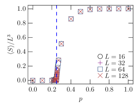
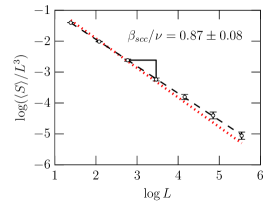
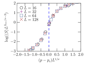
Figure 9: These results correspond to a cubic lattice where each possible directed bond is occupied with probability $p$, with opposite bonds between the same pair of sites being present with probability $p^{2}$, as parameterized in Eq. (13). a) The order parameter for percolation of isotropically directed bonds, corresponding to the fraction occupied by the largest SCC. b) At the critical point, the fraction occupied by the largest cluster decays as a power law, yielding the exponent $\beta_{scc}/\nu$. The red dotted line corresponds to the form $L^{-2\beta/\nu}$, with $\beta=0.418$ and $\nu=0.876$ being the exponents for standard percolation in 3D. Given the error bar of the points and the possibility of finite size deviations, our results allow for the possibility that in three dimensions $\beta_{scc}=2\beta$. c) Using the value obtained for $\beta_{scc}/\nu=0.87$, and assuming that the exponent $\nu=0.876$ as in standard percolation, we can collapse all the curves near the critical point.

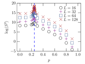
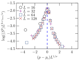
Figure 10: These results correspond to a cubic lattice where each possible directed bond is occupied with probability $p$, with opposite bonds between the same pair of sites being present with probability $p^{2}$, as parameterized in Eq. (13). a) The second moment of the distribution of sizes of SCCs, excluding the largest SCC. b) At the critical point, the second moment grows as a power law, yielding the exponent $\gamma_{scc}/\nu$. c) Using the value obtained for $\gamma_{scc}/\nu$, and assuming $\nu=0.876$ as in standard percolation, we can collapse all the curves near the critical point.

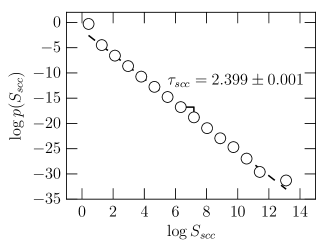
Figure 11: Scaling behavior of the SCC size distribution $p\left(S\right)$ for a cubic lattice with $L=128$, under the second parameterization.

V Discussion

We investigated the percolation of isotropically directed bonds, and presented a conjectured expression for the location of the percolation threshold, which we showed to be exact for the square, triangular and honeycomb lattices.

We have also performed extensive computer simulations and investigated the percolation properties of the strongly-connected components (SCC), the out-components (OUT) and the in-components (IN). Contrary to what happens in directed scale-free networks (Schwartz et al., 2002), on the regular lattices considered in this paper the percolation threshold is the same for SCCs, OUTs and INs. This is related to the fact that, once we are slightly above $p_{c}$, there is an infinite number of paths (in the thermodynamic limit) connecting the opposite sides of the lattice. We also obtain an apparently universal order-parameter exponent for the SCCs that is larger (or, equivalently, a fractal dimension which is smaller) than the one for both the OUTs and the INs. Moreover, the exponents obtained for the giant out-components are the same as those obtained for standard percolation (Zhou et al., 2012). This is in agreement with an approximate real-space renormalization group prediction Redner (1981) that the order-parameter exponents are different for clusters which can be traversed only in one direction and for clusters which can be traversed in both directions. Also, simulations in a cubic lattice allowed us to confirm that the critical point for this case also coincides with that of standard percolation. Finite-size scaling for this case shows that the exponent $\nu$ is the same as that of standard percolation, while the exponents $\beta_{scc}$ and $\gamma_{scc}$ for the giant strongly connected component in percolation of isotropically directed bonds differ from those of standard percolation.

Note that the value of the order-parameter exponent obtained for the SCCs from Figs 4(b) and 5(b) is also distinct from the value of the GOUT order-parameter exponent obtained in Refs. (Inui et al., 1999; Hans-Karl Janssen and Olaf Stenull, 2000) as a function of the anisotropy introduced by allowing a preferred direction. In that case, the exponent is simply given by the product of a crossover exponent and the usual GOUT exponent of standard percolation.

The correlation function gives the probability that two sites separated by a distance $r$ belong to the same cluster and, at the critical transition, decays for large distances r as $g(r)\sim r^{-2\beta/\nu}$  Fisher (1974); Kim Christensen (2005). In the case of percolation of directed bonds, different correlation functions can be defined. Here we define $g_{out}(r)$ as the probability that a given node is in the out-component of another node separated by a distance $r$. Alternatively, we define $g_{scc}(r)$ as the probability that two sites separated by a distance $r$ belong to the same SCC. Assuming that finding a path in one direction or the other are uncorrelated events, we have $g_{scc}(r)=g_{out}(r)\times g_{in}(r)$. Since the in/out components are in the same universality class as standard percolation, we have that, considering uncorrelated events, the value of $\beta_{scc}$ should be twice that for standard percolation. If in fact these events are correlated, one could expect $\beta_{scc}/2$ to be smaller than the exponent $\beta$ of standard percolation. In standard percolation, a cutting bond (Coniglio, 1982) is a bond that if removed results in the loss of connection in a cluster. In our extension, a directed bond can be a cutting bond in each direction or possible in both directions, we call this later case a double cutting bond. The presence of double cutting bonds should lead to correlations between the connectivity events in the opposite directions. Note that the same event (including/removing this cutting bond) would determine the presence or not of a path from one side to the other in both directions. In standard percolation the density of cutting bonds decays as $L^{1/\nu-d}$ (Coniglio, 1982). Considering that being a cutting bond in each direction are independent events, the density of these double cutting bonds should be the square of the density of cutting bonds in standard percolation $L^{2/\nu-2d}$. Since this density decreases faster than $L^{-d}$, the number of such double cutting bonds should be zero in large enough lattice sizes, indicating that no correlation should be observed. In the case of two dimensions this relation is true within the error bars, $\beta_{scc}=0.27\pm 0.01\approx 2\times 5/36=0.2777$. In the case of three dimensions, the obtained value for $\beta_{scc}=0.76\pm 0.08$ is smaller than expected, as the value of standard percolation is $\beta=0.418\pm 0.001$ Ballesteros et al. (1999). However, this deviation is still within the error bars and may also arise from finite-size effects.