Supervised Kernel PCA For Longitudinal Data

Abstract

In statistical learning, high covariate dimensionality poses challenges for robust prediction and inference. To address this challenge, supervised dimension reduction is often performed, where dependence on the outcome is maximized for a selected covariate subspace with smaller dimensionality. Prevalent dimension reduction techniques assume data are i.i.d., which is not appropriate for longitudinal data comprising multiple subjects with repeated measurements over time. In this paper, we derive a decomposition of the Hilbert-Schmidt Independence Criterion as a supervised loss function for longitudinal data, enabling dimension reduction between and within clusters separately, and propose a dimensionality-reduction technique, sklPCA, that performs this decomposed dimension reduction. We also show that this technique yields superior model accuracy compared to the model it extends.

1 Introduction

High covariate (feature) dimensionality poses challenges for robust prediction and inference, and dimensionality reduction is often performed to address this challenge. Supervised dimensionality reduction techniques [BHPT06] attempt to preserve the dependence of the outcome on a reduced covariate subspace while minimizing the dimensionality of that subspace. Supervised kernel dimension reduction (SKDR) methods provide increased flexibility in specifying the relationship between covariates and outcomes by determining the distance metric between points in an implied (often high-dimensional) Hilbert space rather than the dependence of covariates and outcomes directly. Gretton et al. [GBSS05] proposed an independence criterion in reproducing kernel Hilbert spaces [SS02], the Hilbert-Schmidt Independence Criterion (HSIC). Many proposed covariate selection methods use penalized feature weighting to optimize dependence via the HSIC [All13] [CSS⁺07] [FL12] [GC03] [SPS14] [WEST03]. A stepwise selection procedure was suggested by Song et al. [SSG⁺12]. The approach by Chen et al. [CSWJ17] seeks to find a covariate subset for which the HSIC is minimized conditional on that set. Other methods yield a selection of feature transformations, such as Barshan et al. [BGAJ11], who propose a method that selects a subset of feature eigenvectors.

Each of these methods assume data are i.i.d. (independent and identically distributed), which is not true for clustered data. Such data arise naturally in the setting of longitudinal data, which consists of repeated measurements on multiple subjects. Mixed model approaches such as generalized estimating equations [HH02] and generalized linear mixed models [MN01] maximize the dependency of features on the outcome while accounting for clustering, and penalized methods such as GLMM LASSO [GT14] enable feature selection in this context. The degree of clustering might be of interest, in which case SKDR methods that maximize clustering have been developed [SSGB07]. In the longitudinal setting, clustering may be considered a nuisance characteristic of the data, where the primary interest is maximizing the dependence between features and the outcome within clusters. To the authors’ knowledge, no literature to date proposes SKDR techniques in the context of longitudinal data.

This paper derives a method for SKDR in the longitudinal data setting, extending the methods proposed by Barshan et al [BGAJ11]. In Section 2, we review the definition of the HSIC and propose a decomposition of the HSIC resulting in fixed and random components. We derive estimators for this decomposition and prove their bias and rate of convergence. We also propose an algorithm for maximizing these estimators while selecting a feature subspace with reduced dimension. In Section 3, we perform a simulation study to evaluate the properties of this method and compare this derivation with existing methods, and apply this method to the Michigan Intern Health Study. We close with final remarks in Section 4.

2 Methods

2.1 Definition and Decomposition of the HSIC

Consider random variables $X$ and $Y$ representing $p$ distinct features and univariate outcomes, respectively. Let $\mathcal{F}$ and $\mathcal{G}$ be separable Hilbert spaces, equipped with reproducing kernels $k:X\times X\rightarrow\mathbb{R}$ and $l:Y\times Y\rightarrow\mathbb{R}$ such that $k(x,x^{\prime})=\langle\varphi(x),\varphi(x^{\prime})\rangle$ and $\ell(y,y^{\prime})=\langle\psi(y),\psi(y^{\prime})\rangle$ for some maps $\varphi:X\rightarrow\mathcal{F}$ and $\psi:Y\rightarrow\mathcal{G}$, where $\langle\cdot,\cdot\rangle$ denotes an inner product. Gretton et al.[GBSS05] suggest a measurement of dependence in terms of kernels for the features and outcomes:

$$\textit{HSIC}(\mathbb{P}_{X,Y},\mathcal{F},\mathcal{G}): =\|\mathbb{E}_{X,Y}[(\varphi(x)-\mu_{\varphi(X)})\otimes(\psi(y)-\mu_{\psi(Y)})]\|^{2}_{\text{HS}}$$ (1)

where $\otimes$ is the tensor product, $\mu_{\varphi(X)}=\mathbb{E}_{X}(\varphi(x))$ and $\mu_{\psi(Y)}=\mathbb{E}_{Y}(\psi(y))$. This may also be formulated in terms of kernel expectations:

$$\textit{HSIC}(\mathbb{P}_{X,Y},\mathcal{F},\mathcal{G}) =\mathbb{E}_{X,X^{\prime},Y,Y^{\prime}}[k(x,x^{\prime})\ell(y,y^{\prime})]$$

$$\hskip 28.45274pt-2\mathbb{E}_{X,Y}[\mathbb{E}_{X^{\prime}}[k(x,x^{\prime})]\mathbb{E}_{Y^{\prime}}[\ell(y,y^{\prime})]]$$

$$\hskip 28.45274pt+\mathbb{E}_{X,X^{\prime}}[k(x,x^{\prime})]\mathbb{E}_{Y,Y^{\prime}}[\ell(y,y^{\prime})]$$ (2)

Random variables $X$ and $Y$ are independent when this value is zero. For i.i.d. data, SKDR consists of minimizing $\text{dim}(\xi(X))$ for some selection or transformation map $\xi$ while maximizing $\textit{HSIC}(\mathbb{P}_{\xi(X),Y},\mathcal{F},\mathcal{G})$.

If a collection of covariate sets is available and a transformation of reduced dimension is desired for each set, Theorem 1 provides a formulation of the joint HSIC in terms of these random variables.

Theorem 1: Let $X_{1}$ and $X_{2}$ be random variables, $\mathcal{F}_{1}$ and $\mathcal{F}_{2}$ be separable Hilbert spaces equipped with kernels $k_{1}:X_{1}\times X_{1}\rightarrow\mathbb{R}$ and $k_{2}:X_{2}\times X_{2}\rightarrow\mathbb{R}$ such that $k_{1}(x_{1},x_{1}^{\prime})=\langle\varphi(x_{1})$, $\varphi(x_{1}^{\prime})\rangle_{\mathcal{F}_{1}}$ and $k_{2}(x_{2},x_{2}^{\prime})=\langle\varphi(x_{2}),\varphi(x_{2}^{\prime})\rangle_{\mathcal{F}_{2}}$ for some feature maps $\varphi_{1}:X_{1}\rightarrow\mathcal{F}_{1}$ and $\varphi_{2}:X_{2}\rightarrow\mathcal{F}_{2}$. Let $X_{1}\oplus X_{2}$ be the direct sum of these random variables, and $\mathcal{F}_{1}\oplus\mathcal{F}_{2}$ be the direct sum of these Hilbert spaces $\mathcal{F}_{1}$ and $\mathcal{F}_{2}$. Also let $Y$, $\mathcal{G}$, $\ell$, and $\psi$ be defined as before. Then:

$$\emph{HSIC}(\mathbb{P}_{X_{1}\oplus X_{2},Y},\mathcal{F}_{1}\oplus\mathcal{F}_{2},\mathcal{G})=\emph{HSIC}(\mathbb{P}_{X_{1},Y},\mathcal{F}_{1},\mathcal{G})+\emph{HSIC}(\mathbb{P}_{X_{2},Y},\mathcal{F}_{2},\mathcal{G}).$$ (3)

Proof for Theorem 1 is provided in the Supplementary Materials. This theorem readily generalizes to any finite collection of random variables. In general, the random variables and kernels used for between- and within-subject terms are arbitrary. Examples of separate covariate sets suitable for these terms would be subject-level demographic information and within-subject repeated measures. In the context of mixed models, model fits are sought in terms of between- and within-group covariates. Consider a general distribution $Z$, representing cluster membership. Theorem 2 provides a decomposition for HSIC for a single covariate set using a generalization of the law of total covariance.

Theorem 2: Let $X$, $Y$, and $Z$ be random variables, $\mathcal{F}$ and $\mathcal{G}$ be separable Hilbert spaces equipped with kernels $k:X\times X\rightarrow\mathbb{R}$ and $l:Y\times Y\rightarrow\mathbb{R}$ such that $k(x,x^{\prime})=\langle\varphi(x),\varphi(x^{\prime})\rangle_{\mathcal{F}}$ and $\ell(y,y^{\prime})=\langle\psi(y),\psi(y^{\prime})\rangle_{\mathcal{G}}$ for some explicit feature maps $\varphi:X\rightarrow\mathcal{F}$ and $\psi:Y\rightarrow\mathcal{G}$. Then:

$$\emph{HSIC}(\mathbb{P}_{X,Y},\mathcal{F},\mathcal{G}) =\underbrace{\left\|\text{Cov}_{Z}(\mu_{\varphi(X\mid z)},\mu_{\psi(Y\mid z)})\right\|_{\text{HS}}^{2}}_{\emph{HSIC}_{\text{fixed}}}+\underbrace{\mathbb{E}_{Z}\left\|\text{Cov}_{X,Y\mid z}(\varphi(x),\psi(y))\right\|_{\text{HS}}^{2}}_{\emph{HSIC}_{\text{random}}}+\zeta(\mathbb{P}_{X,Y,Z},\mathcal{F},\mathcal{G}).$$ (4)

Theorem 2 is proven in the Supplementary Materials. In this equation, $\zeta(\mathbb{P}_{X,Y,Z},\mathcal{F},\mathcal{G})$ is a nuisance cross-covariance term. In the context of mixed models, the first two terms represent the dependence of the outcome on fixed effects and random effects, respectively. Estimates of these terms may then be used in turn to reduce the dimensions of the fixed effect and random effect covariates.

The estimands of interest in Theorem 2 can also be cast in terms of Theorem 1, by treating these estimands as separate subspaces. Theorem 1 assumes that the total HSIC term is a direct sum of random variables and Hilbert spaces, and any covariance between these terms is assumed to be zero. In mixed regression models, fixed and random effects are typically modeled as independent of each other; we therefore restrict our attention to maximizing the first two terms in Theorem 2. In this paper, we consider the decomposition of a single covariate set only.

2.2 Estimators of HSIC

With our estimands defined, we now derive estimators of these quantities. Let subjects $i=1,...,m$ have repeated measurements $j=1,...,n_{i}$, comprising $n:=\sum_{i=1}^{m}n_{i}$ observations in total. For Subject $i$, let observation $j$ with $p$ features be written $\mathbf{x}_{ij}:=[x_{ij1},...,x_{ijp}]$, let $\mathbf{X}_{i}:=[\mathbf{x}_{i1}^{\top},...,\mathbf{x}_{in_{i}}^{\top}]^{\top}$ be a $n_{i}\times p$ matrix of feature data for Subject $i$, and let feature data for all subjects be written $\mathbf{X}_{n\times p}:=[\mathbf{X}_{1}^{\top},...,\mathbf{X}_{m}^{\top}]^{\top}$. Similarly, let $\mathbf{Y}_{i}:=[y_{1},...,y_{n_{i}}]^{\top}$ and $\mathbf{Y}:=[\mathbf{Y}_{1}^{\top},...,\mathbf{Y}_{m}^{\top}]^{\top}$ represent the outcome data. Let $\mathbf{K}$ and $\mathbf{L}$ be the sample kernels for all observations, where $\mathbf{K}_{i,i^{\prime}}=k(\mathbf{X}_{i,\cdot},\mathbf{X}_{i^{\prime},\cdot})$ and $\mathbf{L}_{i,i^{\prime}}=\ell(\mathbf{Y}_{i},\mathbf{Y}_{i^{\prime}})$, respectively. Finally, let $\mathbf{1}_{m}:=[1,...,1]^{\top}_{m\times 1}$, and $\mathbf{I}_{m}:=\text{diag}(\boldsymbol{1}_{m})$, and let the $m\times m$ centering matrix be defined as $\mathbf{H}_{m}:=\mathbf{I}_{m}-m^{-1}\mathbf{1}_{m}\mathbf{1}_{m}^{\top}$.

Fixed Effects

Let selection matrix $\mathbf{S}_{i}$ be defined as:

$$\mathbf{S}_{i} :=\begin{bmatrix}\mathbf{0}_{(\sum_{i^{\prime}<i}n_{i^{\prime}})\times n_{i}}\\ \mathbf{I}_{n_{i}}\\ \mathbf{0}_{(\sum_{i<i^{\prime}}n_{i^{\prime}})\times n_{i}}\\ \end{bmatrix}$$ (5)

For matrix $\mathbf{W}_{n\times n}$, $\mathbf{S}_{i}^{\top}\mathbf{W}$ and $\mathbf{W}\mathbf{S}_{i}$ result in the selection of the rows and columns associated with Subject $i$, respectively. Let $\overline{k}_{i,i^{\prime}}:=\mathbb{E}_{X\mid z_{i},X^{\prime}\mid z_{i^{\prime}}}\left[k(x,x^{\prime})\right]$ and $\overline{\ell}_{i,i^{\prime}}:=\mathbb{E}_{Y\mid z_{i},Y^{\prime}\mid z_{i^{\prime}}}\left[\ell(y,y^{\prime})\right]$. We define the kernel sample mean between two subjects $i$ and $i^{\prime}$ as follows:

$$\overline{\mathbf{K}}_{i,i^{\prime}} :=(n_{i}-1)^{-1}(n_{i^{\prime}}-1)^{-1}\mathbf{1}_{n_{i}}^{\top}\mathbf{S}_{i}^{\top}\mathbf{K}\mathbf{S}_{i^{\prime}}\mathbf{1}_{n_{i^{\prime}}}$$ (6)

$$\overline{\mathbf{L}}_{i,i^{\prime}} :=(n_{i}-1)^{-1}(n_{i^{\prime}}-1)^{-1}\mathbf{1}_{n_{i}}^{\top}\mathbf{S}_{i}^{\top}\mathbf{L}\mathbf{S}_{i^{\prime}}\mathbf{1}_{n_{i^{\prime}}}$$ (7)

Let $\overline{\mathbf{K}}_{m}:=[\overline{\mathbf{K}}_{i,i^{\prime}}]_{m\times m}$ and $\overline{\mathbf{L}}_{m}:=[\overline{\mathbf{L}}_{i,i^{\prime}}]_{m\times m}$. We propose the following estimator for $\emph{HSIC}_{\text{fixed}}$:

Theorem 3: Under regulatory conditions, then $\widehat{\text{HSIC}}_{\emph{fixed}}:=(m-1)^{-2}\emph{tr}(\overline{\mathbf{K}}_{m}\mathbf{H}_{m}\overline{\mathbf{L}}_{m}\mathbf{H}_{m})$ is a consistent estimator of $\text{HSIC}_{\emph{fixed}}$ with bias of order $\mathcal{O}(m^{-1})$ and convergence rate $\mathcal{O}(m^{-1/2})$.

Proof for Theorem 3 is provided in the Supplementary Materials.

2.2.1 Random Effects

For random effects, we must specify the within-subject correlation structure, analogous to choosing a covariance structure in mixed estimation [ZLRS98]. For example, conditional independence holds if within-subject observations are independent, a strong but common assumption. The following estimator assumes conditional independence holds. Let $\mathbf{K}_{i}:=\mathbf{S}_{i}^{\top}\mathbf{K}\mathbf{S}_{i}$ and $\mathbf{L}_{i}:=\mathbf{S}_{i}^{\top}\mathbf{L}\mathbf{S}_{i}$. A simple unbiased estimator for the expected covariance across subjects is the sample average of subject estimates:

$$\widehat{\emph{HSIC}}_{\text{random}}=m^{-1}\sum_{i=1}^{m}(n_{i}-1)^{-2}\text{tr}\left(\mathbf{K}_{i}\mathbf{H}_{n_{i}}\mathbf{L}_{i}\mathbf{H}_{n_{i}}\right)\\$$ (8)

Theorems 1 and 3 in [GBSS05] imply that the summands in $\widehat{\emph{HSIC}}_{\text{random}}$ each exhibit bias of order $\mathcal{O}(n_{i}^{-1})$ and convergence with rate $\mathcal{O}(n_{i}^{-1/2})$. In terms of Theorem 1, we can combine both HSIC terms into a single estimator by treating them as the direct sum of their respective spaces:

$$\widehat{\emph{HSIC}}_{\text{mixed}} :=\widehat{\emph{HSIC}}_{\text{fixed}}+\widehat{\emph{HSIC}}_{\text{random}}$$ (9)

$$=\text{tr}((m-1)^{-2}\overline{\mathbf{K}}_{m}\mathbf{H}_{m}\overline{\mathbf{L}}_{m}\mathbf{H}_{m})+m^{-1}\sum_{i=1}^{m}\ (n_{i}-1)^{-2}\text{tr}(\mathbf{K}_{i}\mathbf{H}_{n_{i}}\mathbf{L}_{i}\mathbf{H}_{n_{i}})$$ (10)

$$=\text{tr}\{(m-1)^{-2}\overline{\mathbf{K}}_{m}\mathbf{H}_{m}\overline{\mathbf{L}}_{m}\mathbf{H}_{m}\ \underset{i}{\bigoplus}\ m^{-1}(n_{i}-1)^{-2}\mathbf{K}_{i}\mathbf{H}_{n_{i}}\mathbf{L}_{i}\mathbf{H}_{n_{i}}\}$$ (11)

Because each of these terms is non-negative and independent, the global maximum of $\widehat{\emph{HSIC}}_{\text{mixed}}$ is the maximum of each component.

2.3 Maximization of HSIC Estimators

To perform SKDR in the $i.i.d.$ case, Section 5.3.2 of Barshan et al.[BGAJ11] proposes selecting the top generalized eigenvectors of $(\mathbf{K}\mathbf{H}_{n}\mathbf{L}\mathbf{H}_{n}\mathbf{K},\mathbf{K})$. We denote this approach as supervised kernel PCA, or skPCA. We now proceed with a similar derivation for closed-form solutions for maximizing $\widehat{\emph{HSIC}}_{\text{mixed}}$ while reducing the dimension of components for use in longitudinal mixed models. Let $\xi_{\text{fixed}}(\mathbf{X})$ and $\xi_{i}(\mathbf{X})$ be to fixed and subject-specific maps of $\mathbf{X}$ with reduced dimension. We seek $\xi_{\text{fixed}}(\mathbf{X}),\{\xi_{i}(\mathbf{X})\}_{n}$ that maximize $\widehat{\emph{HSIC}}_{\text{mixed}}$ while minimizing $\text{dim}\large(\xi_{\text{fixed}}(\mathbf{X})\large)$, $\text{dim}\large(\{\xi_{i}(\mathbf{X})\}_{n}\large)$.

2.3.1 Fixed Effects

Consider feature map $\overline{\varphi}$ that yields the subject-level mean of $\varphi(\mathbf{X})$ such that $\overline{\mathbf{K}}_{m}=\overline{\varphi}(\mathbf{X})\overline{\varphi}(\mathbf{X})^{\top}$. Let $\mathbf{U}$ be a operator from $\overline{\varphi}$ to the subspace of $\overline{\varphi}$ spanned by $\overline{\varphi}(\mathbf{X})$. Then $\overline{\mathbf{K}}_{m}$ can be rewritten as $\overline{\varphi}(\mathbf{X})\mathbf{U}\mathbf{U}^{\top}\overline{\varphi}(\mathbf{X})^{\top}$. Using the Representer Theorem [KW71], let $\mathbf{U}$ be written as a linear combination $\overline{\varphi}(\mathbf{X})^{\top}\overline{\mathbf{V}}_{m}$. Then $\overline{\mathbf{K}}_{m}=\overline{\varphi}(\mathbf{X})\overline{\varphi}(\mathbf{X})^{\top}\overline{\mathbf{V}}_{m}\overline{\mathbf{V}}_{m}^{\top}\overline{\varphi}(\mathbf{X})\overline{\varphi}(\mathbf{X})^{\top}$, and the fixed component estimator can be written as follows:

$$\widehat{\emph{HSIC}}_{\text{fixed}} =(m-1)^{-2}\text{tr}\left(\overline{\mathbf{K}}_{m}\mathbf{H}_{m}\overline{\mathbf{L}}_{m}\mathbf{H}_{m}\right)$$ (12)

$$=(m-1)^{-2}\text{tr}(\overline{\varphi}(\mathbf{X})\overline{\varphi}(\mathbf{X})^{\top}\overline{\mathbf{V}}_{m}\overline{\mathbf{V}}_{m}^{\top}\overline{\varphi}(\mathbf{X})\overline{\varphi}(\mathbf{X})^{\top}\mathbf{H}_{m}\overline{\mathbf{L}}_{m}\mathbf{H}_{m})$$ (13)

$$=(m-1)^{-2}\text{tr}\left(\overline{\mathbf{V}}_{m}^{\top}\overline{\varphi}(\mathbf{X})\overline{\varphi}(\mathbf{X})^{\top}\mathbf{H}_{m}\overline{\mathbf{L}}_{m}\mathbf{H}_{m}\overline{\varphi}(\mathbf{X})\overline{\varphi}(\mathbf{X})^{\top}\overline{\mathbf{V}}_{m}\right)$$ (14)

$$=(m-1)^{-2}\text{tr}(\overline{\mathbf{V}}_{m}^{\top}\underbrace{\overline{\mathbf{K}}_{m}\mathbf{H}_{m}\overline{\mathbf{L}}_{m}\mathbf{H}_{m}\overline{\mathbf{K}}_{m}}_{\overline{\mathbf{Q}}_{m}}\overline{\mathbf{V}}_{m})$$ (15)

subject to $\overline{\mathbf{V}}_{m}^{\top}\overline{\mathbf{K}}_{m}\overline{\mathbf{V}}_{m}=\mathbf{I}_{m}$. Solving for $\overline{\mathbf{V}}_{m}$ is characterized as the generalized eigenvector problem for matrices ($\overline{\mathbf{Q}}_{m}$, $\overline{\mathbf{K}}_{m}$). Selecting a subset of these generalized eigenvectors with the largest eigenvalues and computing the kernel composed from training and test features, we may compute the resulting feature subspace that maximizes $\widehat{\emph{HSIC}}_{\text{fixed}}$ for any number of reduced dimensions.

2.3.2 Random Effects

Maximizing $\widehat{\emph{HSIC}}_{\text{random}}$ is performed in a similar manner. Let $\mathbf{V}_{i}$ be similarly defined for all $i$:

$$\widehat{\emph{HSIC}}_{\text{random}} =m^{-1}\sum_{i=1}^{m}(n_{i}-1)^{-2}\text{tr}\left(\mathbf{K}_{i}\mathbf{H}_{n_{i}}\mathbf{L}_{i}\mathbf{H}_{n_{i}}\right)$$ (16)

$$=m^{-1}\sum_{i=1}^{m}(n_{i}-1)^{-2}\text{tr}((\varphi(\mathbf{X}_{i})\varphi(\mathbf{X}_{i})^{\top}\mathbf{V}_{i}\mathbf{V}_{i}^{\top}\varphi(\mathbf{X}_{i})^{\top}\varphi(\mathbf{X}_{i})\mathbf{H}_{n_{i}}\mathbf{L}_{i}\mathbf{H}_{n_{i}})$$ (17)

$$=m^{-1}\sum_{i=1}^{m}(n_{i}-1)^{-2}\text{tr}\left(\mathbf{V}_{i}^{\top}\varphi(\mathbf{X}_{i})\varphi(\mathbf{X}_{i})^{\top}\mathbf{H}_{n_{i}}\mathbf{L}_{i}\mathbf{H}_{n_{i}}\varphi(\mathbf{X}_{i})\varphi(\mathbf{X}_{i})^{\top}\mathbf{V}_{i}\right)$$ (18)

$$=m^{-1}\sum_{i=1}^{m}(n_{i}-1)^{-2}\text{tr}(\mathbf{V}_{i}^{\top}\underbrace{\mathbf{K}_{i}\mathbf{H}_{n_{i}}\mathbf{L}_{i}\mathbf{H}_{n_{i}}\mathbf{K}_{i}}_{\mathbf{Q}_{i}}\mathbf{V}_{i})$$ (19)

subject to $\mathbf{V}_{i}^{\top}\mathbf{K}_{i}\mathbf{V}_{i}=\mathbf{I}_{m}\ \forall i$. Because each term in $\widehat{\emph{HSIC}}_{\text{mixed}}$ is positive, it is maximized when its individual summands are maximized. These steps comprise sklPCA, summarized in Algorithm 1.

INPUT: Training features $\mathbf{X}_{n\times p}$, training outcomes $\mathbf{Y}_{n\times 1}$, kernels $k$ and $l$, desired dimensionality $q$ and $q_{i^{*}}$, and test data $\mathbf{X}_{\text{test}}$ with dimension $n_{i^{*}}\times p$ for Subject $i^{*}$.

[.1cm] OUTPUT: Reduced feature data $\xi_{\text{fixed}}(\mathbf{X}_{\text{test}}),\{\xi_{i^{*}}(\mathbf{X}_{\text{test}})\}_{n}$.

1. Compute $\overline{\mathbf{K}}_{i,i^{\prime}}$ and $\overline{\mathbf{L}}_{i,i^{\prime}}\ \forall i,i^{\prime}=1,...,m$.

2. Compute kernels $\overline{\mathbf{K}}_{m}$, $\overline{\mathbf{L}}_{m}$, $\mathbf{K}_{i}$, $\mathbf{L}_{i}\ \forall i=1,...,m$.

3. Compute $\overline{\mathbf{Q}}_{m}:=\overline{\mathbf{K}}_{m}\mathbf{H}_{m}\overline{\mathbf{L}}_{m}\mathbf{H}_{m}\overline{\mathbf{K}}_{m}$ and $\mathbf{Q}_{i}:=\mathbf{K}_{i}\mathbf{H}_{n_{i}}\mathbf{L}_{i}\mathbf{H}_{n_{i}}\mathbf{K}_{i}\ \forall i$.

4. Compute $\overline{\mathbf{V}}_{m}$ := top $q$ generalized eigenvectors from $(\overline{\mathbf{Q}}_{m},\overline{\mathbf{K}}_{m})$.

5. Compute $\mathbf{V}_{i}$ := top $q_{i}$ generalized eigenvectors from $(\mathbf{Q}_{i},\mathbf{K}_{i})\ \forall i$.

6. Compute random test kernel $\mathbf{K}_{i^{*}}:=k(\mathbf{X}_{i^{*}},\mathbf{X}_{i})\ \forall i=1,...,m$.

7. Compute fixed test kernel $\overline{\mathbf{K}}_{m^{*}}:=[(n_{i}-1)^{-1}(n_{i^{*}}-1)^{-1}\mathbf{1}_{n_{i}}^{\top}\mathbf{K}_{i^{*}}\mathbf{1}_{n_{i^{*}}}]_{m}$.

8. Compute $\xi_{\text{fixed}}(\mathbf{X}_{\text{test}})$ := $\overline{\mathbf{K}}_{m^{*}}\overline{\mathbf{V}}_{m}$.

9. $\exists\ i\ (i^{*}=i)$:

10. Compute $\xi_{i^{*}}(\mathbf{X}_{\text{test}})$ := $\mathbf{K}_{i^{*}}\mathbf{V}_{i}$.

Algorithm 1 sklPCA: Perform supervised kernel dimension reduction for longitudinal data.

3 Application

In this section, we demonstrate the utility of sklPCA as a supervised kernel dimension reduction method in a longitudinal setting by applying sklPCA to simulated and empirical datasets, and compare its performance to skPCA.

3.1 Simulation Specification

We construct a simulation that satisfies the following conditions: (1) features and outcomes are measured multiple times for several subjects exhibiting within-subject clustering, (2) the relationship between features within and between subjects and the outcome is arbitrary, and (3) features are sampled from a high-dimensional, low-rank space. The modeling task in this simulation is to reduce the dimensionality of these high-dimensional features resulting in between-subject and within-subject components appropriate for use in a mixed model. To elucidate circumstances under which sklPCA and/or skPCA perform well in this task, we repeat the simulation study under a variety of simulated settings.

For subjects $i=1,...,m$ at measurement time $j=1,...,n_{i}$, the outcome of interest $\widetilde{\mathbf{Y}}_{ij}$ depends on a subspace $\widetilde{\mathbf{X}}_{ij}$ though an arbitrary function $f_{Y}$ in a way that differs between and within subjects. The observed outcomes $\mathbf{Y}_{ij}$ are assumed to be noisy measurements of $\widetilde{\mathbf{Y}}_{ij}$, and the observed features $\mathbf{X}_{ij}$ are related to $\widetilde{\mathbf{X}}_{ij}$ linearly through a projection matrix $\mathbf{P}$ with rank $R$ and dimension $D$, where $R\ll D$. The distributional form of these variables are specified as follows:

$$\mathbf{Y}_{ij} =\underbrace{f_{Y}(\widetilde{\mathbf{X}}_{ij},\boldsymbol{\mu}_{i};\sigma_{w})-f_{Y}(\boldsymbol{\mu}_{i},\boldsymbol{0}_{R};\sigma_{b})}_{\widetilde{\mathbf{Y}}_{ij}}+\epsilon_{ij},\quad\epsilon_{ij}\sim\mathcal{N}(0,\sigma^{2}_{\epsilon})$$ (20)

$$\hskip 56.9055pt\boldsymbol{\mu}_{i} \sim f_{\mu}(\mathbf{0}_{k},\sigma_{b}^{2}\mathbb{I}_{R}),\quad i=1,...,m$$ (21)

$$\widetilde{\mathbf{X}}_{ij} \sim f_{X}(\boldsymbol{\mu}_{i},\sigma_{w}^{2}\mathbb{I}_{R}),\quad j=1,...,n_{i}$$ (22)

$$\mathbf{X}_{ij} =\mathbf{P}^{\top}\widetilde{\mathbf{X}}_{ij},\quad\mathbf{P}\sim\mathcal{N}(0,1)^{R\times D}$$ (23)

3.2 Model Comparison

We vary four binary factors independently: (1) $\sigma_{b}/\sigma_{w}$, or the ratio of between-subject variance compared to within-subject variance, (2) two configurations of distributions applied in the above framework, (3) the rank of the predictors $R$, and (4) the dimension of the predictors $D$. The two distribution configurations are selected to imitate linear and non-linear relationships, respectively:

1. Linear Configuration: $f_{\mu},f_{X}$ are uniform, where the support is defined on $\prod_{r=1}^{R}[\boldsymbol{\mu}_{r}\pm\sqrt{3}\sigma]$ to preserve mean $\boldsymbol{\mu}$ and variance $\sigma^{2}\mathbb{I}_{R}$. $f_{Y}^{(\text{linear})}(\mathbf{x},\boldsymbol{\mu};\sigma)=\sum_{r=1}^{R}(\mathbf{x}_{r}-\boldsymbol{\mu}_{r})$, and kernels $k$ and $l$ are set to the linear kernel $\kappa(\mathbf{\mathbf{w},\mathbf{w}^{\prime}};\sigma)=\mathbf{w}^{\top}\mathbf{w}^{\prime}$.

2. Radial Configuration: $f_{\mu},f_{X}$ are standard normal, and $f_{Y}$, $k$, and $l$ are set to the Gaussian radial kernel, $\kappa(\mathbf{w},\mathbf{w}^{\prime};\sigma)=\exp\left(-\frac{1}{2\sigma^{2}}\left\|(\mathbf{w}-\mathbf{w}^{\prime})\right\|^{2}_{2}\right)$.

Variants of these distribution configurations are displayed visually in Figure 1; the above configurations correspond to the diagonal panels. Note that $f_{Y}=f_{Y}^{(\text{linear})}$ specifies a high-dimensional linear mixed model, whereas $f_{Y}=f_{Y}^{(\text{radial})}$ specifies a more complex relationship for which more flexible methods such as SKDR is required. The selection of the remaining parameters are $\sigma_{b}/\sigma_{w}\in\{0.1,1\}$, $R\in\{1,5\}$, and $D\in\{10,1000\}$. For each combination, several other parameters are held constant. To enable arbitrarily accurate model fits when the model is appropriately specified, the error between the outcome and latent space is assumed to be very low, $\sigma^{2}_{\epsilon}=1e-5$. The data are assumed to exhibit moderate size, $m=n_{i}=50$; for simplicity, we assume $n_{i}$ is the same for all subjects.

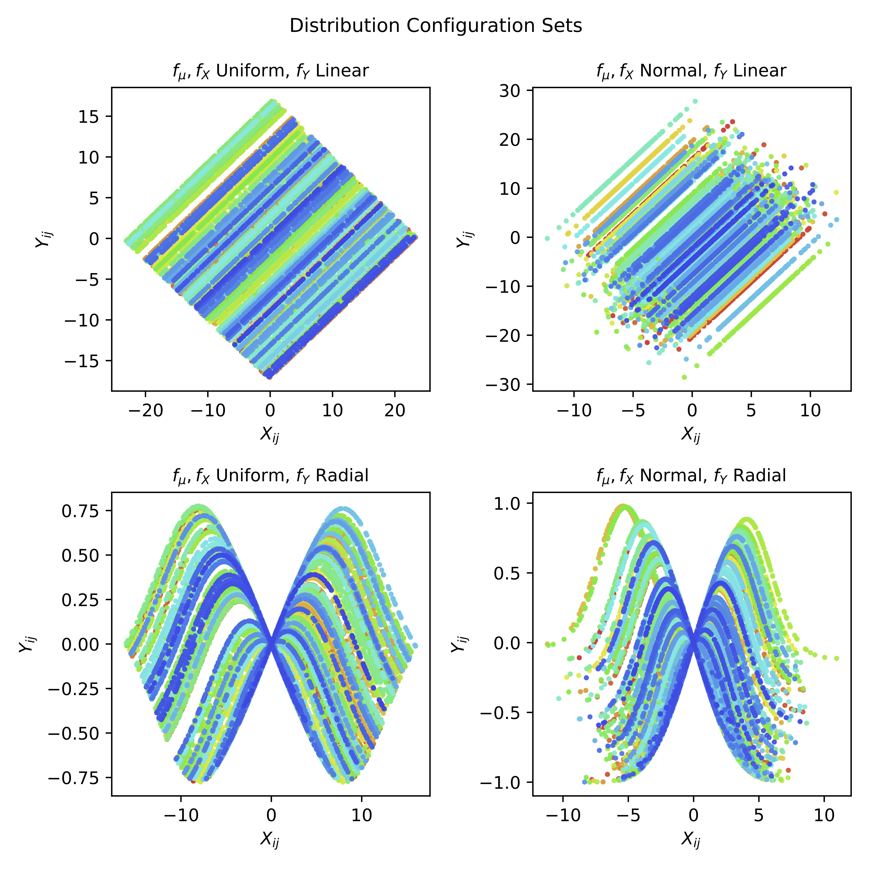
Figure 1: Sample datasets using the simulation framework described in this section. The lefthand panels assume $f_{\mu},f_{X}$ are distributed uniformly, whereas the righthand panels assume $f_{\mu},f_{X}$ are distributed normally. The top panels assume $f_{Y}$ is linear, and the bottom panels assume $f_{Y}$ takes the form of the Gaussian radial basis function. Individual colors represent separate subjects, and individual points represent feature/outcome measurement pairs. In this figure, $R=D=1$ and $m=n_{i}=150$ are assumed.

After simulation and dimension reduction, linear and mixed regression models are fit to the data reduced using skPCA and sklPCA, respectively. The mixed models are fit using a two-step estimation approach similar to the unrestricted estimation of longitudinal models [Ver97], which is performed by first reducing and fitting the fixed component, then reducing and fitting the random components to the resulting residuals. The criterion of 5-fold cross-validated correlation between the predictions and outcome is used to compare results across each simulation and method. Each parameter combination is simulated 100 times, and the sample mean and standard deviation of the out-of-sample prediction correlations is calculated. Simulations were performed on a 15-inch 2017 MacBook Pro laptop computer, with a 2.8 GHz Intel Core i7 processor (4 cores) and 16 GB RAM. The results of these analyses are shown in Table 1.

The general form of $\widetilde{Y}_{ij}$ is designed to produce no little or no correlation when $\sigma_{b}=\sigma_{w}$ if subject identity is not taken into account, because the relationship between subjects is the negative of that within each subject. This results in poor model performance when using skPCA, which treats each observation independently, whereas sklPCA reduces the feature dimension separately based on these separate relationships. When the between-subject variance is small ($\sigma_{b}/\sigma_{w}=0.1$), skPCA performs reasonably well, although sklPCA still yields superior accuracy. Due to the increased complexity, the radial configuration is less performant than the linear configuration. Because the dataset size is held constant, increasing the rank of the feature space has the intuitive effect of reducing overall predictive performance. In contrast, the effect of increasing the dimensionality of the feature space differs for the two distribution configurations: model performance is maintained or slightly improves in the linear case, but model performance decreases in the radial case, and the size of the effect is monotone in $R$ and $D$. For moderate-sized data, determining complex non-linear relationships is particularly challenging in high-rank, high-dimensional settings.

		Linear Configuration				Radial Configuration
		$\sigma_{b}/\sigma_{w}=0.1$		$\sigma_{b}/\sigma_{w}=1$		$\sigma_{b}/\sigma_{w}=0.1$		$\sigma_{b}/\sigma_{w}=1$
$R=1$	$D=10$	0.979	(0.003)	0.050	(0.050)	0.601	(0.051)	0.056	(0.049)	skPCA
		0.999	($<$1e-3)	0.971	(0.004)	0.885	(0.011)	0.765	(0.034)	sklPCA
3-10	$D=1000$	0.980	(0.002)	0.046	(0.037)	0.595	(0.056)	0.044	(0.047)	skPCA
		0.999	($<$1e-3)	0.972	(0.003)	0.785	(0.024)	0.631	(0.047)	sklPCA
$R=5$	$D=10$	0.861	(0.082)	0.124	(0.047)	0.674	(0.046)	0.245	(0.043)	skPCA
		0.991	(0.005)	0.905	(0.035)	0.813	(0.027)	0.667	(0.030)	sklPCA
3-10	$D=1000$	0.964	(0.017)	0.135	(0.062)	0.629	(0.033)	0.006	(0.025)	skPCA
		0.998	($<$1e-3)	0.958	(0.005)	0.573	(0.048)	0.021	(0.014)	sklPCA

Table 1: Simulation results. Cells represent simulation results varying $\sigma_{b}/\sigma_{w}$, distribution configuration, rank $R$, and dimension $D$ independently, comparing skPCA and sklPCA, where the latter is denoted in bold. Within each cell, mean out-of-sample prediction correlations across 100 repeated simulations is shown on the left (with standard deviations shown in parentheses on the right).

To illustrate performance differences between these methods, we performed additional simulations designed for visual clarity (see Figure 2). The relationships between $\widetilde{\mathbf{X}}_{ij}$ and $\widetilde{\mathbf{Y}}_{ij}$ are constructed to produce a regular lattice: $\mu_{i}=\sigma_{b}\left(\frac{i}{m}-\frac{1}{2}\right)$, $\widetilde{X}_{ij}=\sigma_{w}\left(\frac{j}{n_{i}}-\frac{1}{2}\right)+\mu_{i}$, and $\widetilde{Y}_{ij}=\sigma_{w}\left(\frac{j}{n_{i}}-\frac{1}{2}\right)-\mu_{i}$. The simulation parameters for this simulation are set as $m=n_{i}=15$, $\sigma_{b}\in\{1,5\}$, $\sigma_{w}\in\{1,5\}$, and $\sigma_{\epsilon}=0.01$. In this figure, perfectly accurate model predictions for all outcomes would yield a diagonal line. For the diagonal panels, the within-subject and between-subject correlations are equal; again, by design, performing data reduction and modeling assuming i.i.d data yields little or no model accuracy in expectation. In contrast, the sklPCA and mixed model approach does capture the within-subject and between-subject correlations separately, resulting in highly accurate cross-validated predictions. The off-diagonal panels show cases where the variance within subjects and between subjects differ markedly. In these cases, the larger variance component will account for an overall correlation between $\widetilde{X}$ and $Y$, even for the i.i.d reduction and modeling strategy. However, Figure 2 shows that predictions using this approach reliably fail to model the remaining correlation resulting from the smaller source of variation; the two sources exhibit correlations of opposite magnitude, and the resulting model fits reveal residuals of potential correlation consistently not captured by this model. In these cases, the sklPCA combined with a mixed model approach successfully models both components, yielding comparatively stronger overall correlations.

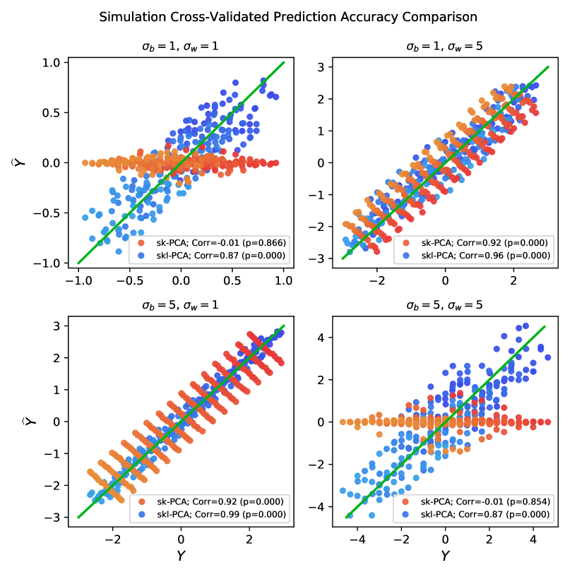
Figure 2: A comparison of model performance for the simulated lattice dataset. The top and bottom panels exhibit a between-subject variance of $\sigma_{b}=1$ and $5$, respectively. Panels on the left side and right side exhibit a within-subject variance of $\sigma_{w}=1$ and $5$, respectively. In each panel, true simulated outcomes $Y$ are shown on the $x$-axis, and model fits $\widehat{Y}$ are shown on the $y$-axis. The green line is the identity; proximity to this line indicates accurate out-of-sample model performance. The red-like dots depict individual out-of-sample skPCA predictions, and shades from red to orange represent different subjects. The blue-like dots depict individual cross-validation sklPCA predictions. In each case, the cross-validated correlation using sklPCA is stronger than skPCA.

3.3 Application to the Michigan Intern Health Study

We now turn to an application of sklPCA to an empirical dataset. The Intern Health Study is a multi-site prospective cohort study following physicians throughout internship, for whom correlations are sought between their internship tenure and cognitive and/or clinical outcomes such as mood [KFA⁺18], depression [SKK⁺10], and suicidal ideation [GZK⁺15]. Residencies among interns range from internal medicine, general surgery, pediatrics, obstetrics/gynecology, and psychiatry.

This cohort has participated in an assortment of experimental interventions and clinical measurements of well-being. Among these, a subset of physicians installed the Mindstrong digital phenotyping app, which unobtrusively collects content-free feature information such as swiping and typing patterns. A variety of feature extraction techniques are subsequently used to reduce the behavioral gestures to a single, high-dimensional set of features per day per subject. This daily measurement is matched with an outcome of interest: the cumulative sum of minutes of sleep obtained within the last 4 days. The measure of accuracy used to measure model performance is out-of-sample cross-validated correlation, where $k=5$ training folds are created by dividing all paired outcome/feature repeated measurements per subject into a partition of $k$ time-contiguous parts each, for which all but one part are used as training data, and the remaining part is used for predictive testing.

Among the 181 consented physicians, 108 installed the Mindstrong app and uploaded sufficient phone log data from which to extract features and reported minutes spent sleeping per day. We perform a complete cases analysis, in which a subset of the data exhibiting no missing values is selected, comprising 575 features and 56 subjects with 1415 total daily outcome/feature pairs. Following Bair et al. [BHPT06], the number of features is further reduced by selecting features with significant univariate correlations while controlling for a false discovery rate of 0.1.

After performing these preprocessing steps, we compare the two methods previously discussed in this section. Employing skPCA yields a cross-validated correlation of 0.438 ($p$<1e-10). While using sklPCA, a cross-validated correlation of 0.814 ($p$<1e-10) is achieved (see Figure 3). Individual predictions over time for a subset of subjects are shown in Figure 4. Combined, these suggest that performing SKDR while accounting for subject identity in longitudinal datasets can result in substantially improved model performance.

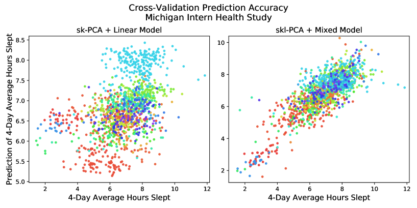
Figure 3: The cross-validated correlation comparing two modeling approaches in the Michigan Intern Health Study. The left panel displays prediction results employing skPCA, and the right panel displays results using sklPCA. The $x$-axis depicts the 4-day average hours slept, and the $y$-axis represents the prediction. Each color represents a distinct subject. skPCA shows less overall cross-validated correlation, as well as between-subject prediction differences that are broadly unrelated to the outcome. sklPCA shows higher cross-validated correlations both within and between subjects.

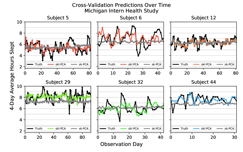
Figure 4: Outcomes and cross-validated model predictions over time for a selection of subjects in the Michigan Intern Health Study. The six panels depict results for a single selected subject each. The $x$-axis shows days for which outcomes and biomarker data were both available for modeling, ordered in time. The $y$-axis shows the 4-day average of sleep for each observation. Black lines show measured sleep averages over time, gray lines show cross-validated predictions using skPCA, and the variously colored lines per panel show cross-validated predictions using sklPCA.

4 Conclusion

We have proposed a supervised kernel dimension reduction method in the longitudinal setting. In Section 2, we derived a novel decomposition for the HSIC, and proposed sklPCA, a method extending skPCA that maximizes two constituent components of HSIC separately. In Section 3, we showed that our method yields comparable or superior accuracy compared to skPCA for a range of simulation settings. We also applied these approaches to the Michigan Intern Health Study, for which sklPCA yielded a cross-validated correlation approximately twice that obtained using skPCA.

This estimation procedure might be improved in several ways. This work extends the HSIC estimator proposed by Gretton et al., [GBSS05], yet more efficient estimators in both the computational and statistical sense have recently been proposed [PSCV17]. Extending this approach for longitudinal data might be similarly efficient. Alternatively, the estimator for the HSIC used here is based on $U$-statistics [Hoe48], which have been extended to non-i.i.d. data [Bor96], which might provide another route through which estimators of the HSIC may be derived for clustered data. Our method transforms covariates by selecting generalized eigenvectors, but techniques for recasting variable transformation methods as feature selection methods have been developed [MDF10], which might be adopted here. Finally, new kernels might be developed that account for within-subject clustering, such as an extension of the Gaussian mixture proposed by Weiss et al. [Wei99]. We leave such investigations as future work.

5 Supplementary Materials

In this supplement, we provide proofs for the theorems stated in the paper.

5.1 Proof of Theorem 1

Theorem 1: Let $X_{1}$, $X_{2}$, and $Y$ be random variables, $\mathcal{F}_{1}$, $\mathcal{F}_{2}$, and $\mathcal{G}$ be separable Hilbert spaces equipped with kernels $k_{1}:X_{1}\times X_{1}\rightarrow\mathbb{R}$, $k_{2}:X_{2}\times X_{2}\rightarrow\mathbb{R}$, and $\ell:Y\times Y\rightarrow\mathbb{R}$ such that $k_{1}(x_{1},x_{1}^{\prime})=\langle\varphi(x_{1})$, $\varphi(x_{1}^{\prime})\rangle_{\mathcal{F}_{1}}$, $k_{2}(x_{2},x_{2}^{\prime})=\langle\varphi(x_{2}),\varphi(x_{2}^{\prime})\rangle_{\mathcal{F}_{2}}$, and $\ell(y,y^{\prime})=\langle\psi(y),\psi(y^{\prime})\rangle_{\mathcal{G}}$ for some explicit feature maps $\varphi_{1}:X_{1}\rightarrow\mathcal{F}_{1}$, $\varphi_{2}:X_{2}\rightarrow\mathcal{F}_{2}$, and $\psi:Y\rightarrow\mathcal{G}$. Let $X_{1}\oplus X_{2}$ be the direct sum of these random variables, and $\mathcal{F}_{1}\oplus\mathcal{F}_{2}$ be the direct sum of these Hilbert spaces $\mathcal{F}_{1}$ and $\mathcal{F}_{2}$. Then:

$$\emph{HSIC}(\mathbb{P}_{X_{1}\oplus X_{2},Y},\mathcal{F}_{1}\oplus\mathcal{F}_{2},\mathcal{G})=\emph{HSIC}(\mathbb{P}_{X_{1},Y},\mathcal{F}_{1},\mathcal{G})+\emph{HSIC}(\mathbb{P}_{X_{2},Y},\mathcal{F}_{2},\mathcal{G}).$$ (24)

Proof: The direct sum of two Hilbert spaces is also a Hilbert space, equipped with the inner product
$\langle x_{1}\oplus x_{2},x_{1}^{\prime}\oplus x_{2}^{\prime}\rangle_{\mathcal{F}_{1}\oplus\mathcal{F}_{2}}:=\langle x_{1},x_{1}^{\prime}\rangle_{\mathcal{F}_{1}}+\langle x_{2}^{\prime},x_{2}^{\prime}\rangle_{\mathcal{F}_{2}}$. The kernel for feature map $\varphi_{1}\oplus\varphi_{2}$ is therefore:

$$k(x_{1}\oplus x_{2},x_{1}^{\prime}\oplus x_{2}^{\prime}) =\langle\varphi_{1}(x_{1})\oplus\varphi_{2}(x_{2}),\varphi_{1}(x_{1}^{\prime})\oplus\varphi_{2}(x_{2}^{\prime})\rangle_{\mathcal{F}_{1}\oplus\mathcal{F}_{2}}$$ (25)

$$=\langle\varphi(x_{1}),\varphi(x_{1}^{\prime})\rangle_{\mathcal{F}_{1}}+\langle\varphi_{2}(x_{2}),\varphi_{2}(x_{2}^{\prime})\rangle_{\mathcal{F}_{2}}$$ (26)

$$=k_{1}(x_{1},x_{1}^{\prime})+k_{2}(x_{2},x_{2}^{\prime})$$ (27)

Let $\mu_{\varphi(X)}:=\mathbb{E}_{X}\left[\varphi(x)\right]=\int_{x}\varphi(x)p_{X}(x)$. Using the linearity of expectations and the distributive properties for direct sums and tensor products, we obtain:

$$\mathbb{E}_{X_{1}\oplus X_{2}}[(\varphi_{1}(x_{1})\oplus\varphi_{2}(x_{2})-\mu_{\varphi_{1}(X_{1})\oplus\varphi_{2}(X_{2})})\otimes(\psi(y)-\mu_{\psi(Y)})]=$$ (28)

$$\mathbb{E}_{X_{1},Y}[(\varphi_{1}(x_{1})-\mu_{\varphi_{1}(X_{1})})\otimes(\psi(y)-\mu_{\psi(Y)})]\oplus\mathbb{E}_{X_{2},Y}[(\varphi_{2}(x_{2})-\mu_{\varphi_{2}(X_{2})})\otimes(\psi(y)-\mu_{\psi(Y)})]=$$ (29)

$$C_{x_{1},y}\oplus C_{x_{2},y}$$ (30)

for cross-covariance linear operators $C_{x_{1},y}:\mathcal{G}\rightarrow\mathcal{F}_{1}$ and $C_{x_{2},y}:\mathcal{G}\rightarrow\mathcal{F}_{2}$. The Hilbert-Schmidt norm of $C_{x_{1},y}\oplus C_{x_{2},y}$ is therefore:

$$\|C_{x_{1},y}\oplus C_{x_{2},y}\|^{2}_{\text{HS}} =\sum_{i,j,k}\langle C_{x_{1},y}\oplus C_{x_{2},y}(v_{i}\oplus w_{j}),u_{k}\rangle_{\mathcal{F}_{1}\oplus\mathcal{F}_{2}}$$ (31)

$$=\sum_{i,k}\langle C_{x_{1},y}v_{i},u_{k}\rangle_{\mathcal{F}_{1}}+\sum_{j,k}\langle C_{x_{2},y}w_{j},u_{k}\rangle_{\mathcal{F}_{2}}$$ (32)

$$=\emph{HSIC}(\mathbb{P}_{X_{1},Y},\mathcal{F}_{1},\mathcal{G})+\emph{HSIC}(\mathbb{P}_{X_{2},Y},\mathcal{F}_{2},\mathcal{G})$$ (33)

$\blacksquare$

5.2 Proof of Theorem 2

Theorem 2: Let $X$, $Y$, and $Z$ be random variables, $\mathcal{F}$ and $\mathcal{G}$ be separable Hilbert spaces equipped with kernels $k:X\times X\rightarrow\mathbb{R}$ and $l:Y\times Y\rightarrow\mathbb{R}$ such that $k(x,x^{\prime})=\langle\varphi(x),\varphi(x^{\prime})\rangle_{\mathcal{F}}$ and $\ell(y,y^{\prime})=\langle\psi(y),\psi(y^{\prime})\rangle_{\mathcal{G}}$ for some explicit feature maps $\varphi:X\rightarrow\mathcal{F}$ and $\psi:Y\rightarrow\mathcal{G}$. Then:

$$\emph{HSIC}(\mathbb{P}_{X,Y},\mathcal{F},\mathcal{G}) =\underbrace{\left\|\text{Cov}_{Z}(\mu_{\varphi(X\mid z)},\mu_{\psi(Y\mid z)})\right\|_{\text{HS}}^{2}}_{\emph{HSIC}_{\text{fixed}}}+\underbrace{\mathbb{E}_{Z}\left\|\text{Cov}_{X,Y\mid z}(\varphi(x),\psi(y))\right\|_{\text{HS}}^{2}}_{\emph{HSIC}_{\text{random}}}+\zeta(\mathbb{P}_{X,Y,Z},\mathcal{F},\mathcal{G}).$$ (34)

Proof: For ease of notation, define the following expectations:

$$\mu_{\varphi(X)} :=\mathbb{E}_{X}\left[\varphi(x)\right]=\int_{x}\varphi(x)p_{X}(x)$$ (35)

$$\mu_{\varphi(X\mid z)} :=\mathbb{E}_{X\mid z}\left[\varphi(x)\right]=\int_{x}\varphi(x)p_{X\mid z}(x\mid z)$$ (36)

Applying these to the cross-covariance operator for $\varphi$ and $\psi$, we obtain:

$$\text{Cov}_{X,Y}(\varphi(x),\psi(y)) =\mathbb{E}_{X,Y}\left[\varphi(x)\otimes\psi(y)\right]-\mu_{\varphi(X)}\otimes\mu_{\psi(Y)}$$ (37)

$$=\mathbb{E}_{Z}\left[\mathbb{E}_{X,Y\mid z}\left[\varphi(x)\otimes\psi(y)\right]\right]-\mathbb{E}_{Z}\left[\mu_{\varphi(X\mid z)}\right]\otimes\mathbb{E}_{Z}\left[\mu_{\psi(Y\mid z)}\right]$$ (38)

$$=\mathbb{E}_{Z}\left[\text{Cov}_{X,Y\mid z}(\varphi(x),\psi(y))+\mu_{\varphi(X\mid z)}\otimes\mu_{\psi(Y\mid z)}\right]-\mathbb{E}_{Z}\left[\mu_{\varphi(X\mid z)}\right]\otimes\mathbb{E}_{Z}\left[\mu_{\psi(Y\mid z)}\right]$$ (39)

$$=\mathbb{E}_{Z}\left[\text{Cov}_{X,Y\mid z}(\varphi(x),\psi(y))\right]+\mathbb{E}_{Z}\left[\mu_{\varphi(X\mid z)}\otimes\mu_{\psi(Y\mid z)}\right]-\mathbb{E}_{Z}\left[\mu_{\varphi(X\mid z)}\right]\otimes\mathbb{E}_{Z}\left[\mu_{\psi(Y\mid z)}\right]$$ (40)

$$=\mathbb{E}_{Z}\left[\text{Cov}_{X,Y\mid z}(\varphi(x),\psi(y))\right]+\text{Cov}_{Z}(\mu_{\varphi(X\mid z)},\mu_{\psi(Y\mid z)})$$ (41)

The norm of (37), or $\emph{HSIC}(\mathbb{P}_{X,Y},\mathcal{F},\mathcal{G})$, decomposes into three terms:

$$\left\|\text{Cov}_{X,Y}(\varphi(x),\psi(y))\right\|^{2}_{\text{HS}} =\left\|\text{Cov}_{Z}(\mu_{\varphi(X\mid z)},\mu_{\psi(Y\mid z)})\right\|_{\text{HS}}^{2}+\left\|\mathbb{E}_{Z}\ \text{Cov}_{X,Y\mid z}(\varphi(x),\psi(y))\right\|_{\text{HS}}^{2}$$

$$\hskip 28.45274pt+2\langle\mathbb{E}_{Z}[\text{Cov}_{X,Y\mid z}(\varphi(x),\psi(y))],\text{Cov}_{Z}(\mu_{\varphi(X\mid z)},\mu_{\psi(Y\mid z)})\rangle_{\text{HS}}$$ (42)

The second term may be evaluated as follows:

$$\left\|\mathbb{E}_{Z}\text{Cov}_{X,Y\mid z}(\varphi(x),\psi(y))\right\|_{\text{HS}}^{2} =\mathbb{E}_{Z}\left\|\text{Cov}_{X,Y\mid z}(\varphi(x),\psi(y))\right\|_{\text{HS}}^{2}$$

$$\hskip 28.45274pt+2\sum_{z<z^{\prime}}\left\langle\text{Cov}_{X,Y\mid z}(\varphi(x),\psi(y)),\text{Cov}_{X,Y\mid z^{\prime}}(\varphi(x),\psi(y))\right\rangle_{\text{HS}}$$ (43)

Therefore, Equation (34) holds upon gathering the cross-covariance terms:

$$\zeta(\mathbb{P}_{X,Y,Z},\mathcal{F},\mathcal{G}):= -2\langle\mathbb{E}_{Z}[\text{Cov}_{X,Y\mid z}(\varphi(x),\psi(y))],\text{Cov}_{Z}(\mu_{\varphi(X\mid z)},\mu_{\psi(Y\mid z)})\rangle_{\text{HS}}$$

$$+2\sum_{z<z^{\prime}}\left\langle\text{Cov}_{X,Y\mid z}(\varphi(x),\psi(y)),\text{Cov}_{X,Y\mid z^{\prime}}(\varphi(x),\psi(y))\right\rangle_{\text{HS}}$$ (44)

$\blacksquare$

5.3 Proof of Theorem 3

Theorem 3: Under regulatory conditions, then $\widehat{\text{HSIC}}_{\emph{fixed}}:=(m-1)^{-2}\emph{tr}(\overline{\mathbf{K}}_{m}\mathbf{H}_{m}\overline{\mathbf{L}}_{m}\mathbf{H}_{m})$ is a consistent estimator of $\text{HSIC}_{\emph{fixed}}$ with bias of order $\mathcal{O}(m^{-1})$ and convergence rate $\mathcal{O}(m^{-1/2})$.

Proof: $\emph{HSIC}_{\text{fixed}}$ may be written in terms of conditional expectations:

$$\emph{HSIC}_{\text{fixed}} =\left\|\text{Cov}_{Z}(\mu_{\varphi(X\mid z)},\mu_{\psi(Y\mid z)})\right\|_{\text{HS}}^{2}$$ (45)

$$=\mathbb{E}_{Z,Z^{\prime}}\left[\mathbb{E}_{X\mid z,X^{\prime}\mid z^{\prime}}\left[k(x,x^{\prime})\right]\mathbb{E}_{Y\mid z,Y^{\prime}\mid z^{\prime}}\left[\ell(y,y^{\prime})\right]\right]$$

$$\hskip 28.45274pt-2\mathbb{E}_{Z}\left[\mathbb{E}_{X\mid z,X^{\prime}}\left[k(x,x^{\prime})\right]\mathbb{E}_{Y\mid z,Y^{\prime}}\left[\ell(y,y^{\prime})\right]\right]$$

$$\hskip 28.45274pt+\mathbb{E}_{X,X^{\prime}}[k(x,x^{\prime})]\mathbb{E}_{Y,Y^{\prime}}[\ell(y,y^{\prime})]$$ (46)

$$=\mathbb{E}_{Z,Z^{\prime}}\left[\mathbb{E}_{X\mid z,X^{\prime}\mid z^{\prime}}\left[k(x,x^{\prime})\right]\mathbb{E}_{Y\mid z,Y^{\prime}\mid z^{\prime}}\left[\ell(y,y^{\prime})\right]\right]$$

$$\hskip 28.45274pt-2\mathbb{E}_{Z}\left[\mathbb{E}_{Z^{\prime}}\left[\mathbb{E}_{X\mid z,X^{\prime}|z^{\prime}}\left[k(x,x^{\prime})\right]\right]\mathbb{E}_{Z^{\prime}}\left[\mathbb{E}_{Y\mid z,Y^{\prime}|z^{\prime}}\left[\ell(y,y^{\prime})\right]\right]\right]$$

$$\hskip 28.45274pt+\mathbb{E}_{Z,Z^{\prime}}\left[\mathbb{E}_{X|z,X^{\prime}|z^{\prime}}[k(x,x^{\prime})]\right]\mathbb{E}_{Z,Z^{\prime}}\left[\mathbb{E}_{Y|z,Y^{\prime}|z^{\prime}}[\ell(y,y^{\prime})]\right]$$ (47)

$\widehat{\emph{HSIC}}_{\text{fixed}}$ may be decomposed as follows:

$$\widehat{\emph{HSIC}}_{\text{fixed}} =(m-1)^{-2}\text{tr}\left(\overline{\mathbf{K}}_{m}\mathbf{H}_{m}\overline{\mathbf{L}}_{m}\mathbf{H}_{m}\right)$$ (48)

$$=(m-1)^{-2}\text{tr}(\overline{\mathbf{K}}_{m}\overline{\mathbf{L}}_{m})+(m-1)^{-3}\mathbf{1}^{\top}\overline{\mathbf{K}}_{m}\overline{\mathbf{L}}_{m}\mathbf{1}+(m-1)^{-4}\mathbf{1}^{\top}\overline{\mathbf{K}}_{m}\mathbf{1}\mathbf{1}^{\top}\overline{\mathbf{L}}_{m}\mathbf{1}$$ (49)

$$=\frac{1}{(m-1)^{2}}\sum_{i,i^{\prime}=1}^{m}\overline{\mathbf{K}}_{i,i^{\prime}}\overline{\mathbf{L}}_{i,i^{\prime}}$$

$$\hskip 28.45274pt+\frac{1}{m}\sum_{i=1}^{m}\frac{1}{(m-1)^{2}}\sum_{i^{\prime},i^{\prime\prime}=1}^{m}\overline{\mathbf{K}}_{i^{\prime},i}\overline{\mathbf{L}}_{i,i^{\prime\prime}}$$

$$\hskip 28.45274pt+\left(\frac{1}{m(m-1)}\sum_{i,i^{\prime}=1}^{m}\overline{\mathbf{K}}_{i,i^{\prime}}\right)\left(\frac{1}{m(m-1)}\sum_{i,i^{\prime}=1}^{m}\overline{\mathbf{L}}_{i,i^{\prime}}\right)$$ (50)

Therefore, $\widehat{\emph{HSIC}}_{\text{fixed}}$ is the sum of $U$-estimators in terms of $\overline{\mathbf{K}}_{i,i^{\prime}}$ and $\overline{\mathbf{L}}_{i,i^{\prime}}$. If these terms are bounded, then by Theorems 1 and 3 in [GBSS05], it follows immediately that $\widehat{\emph{HSIC}}_{\text{fixed}}$ has bias $\mathcal{O}(m^{-1})$ and converges to $\emph{HSIC}_{\text{fixed}}$ with rate $\mathcal{O}(m^{-1/2})$.

As $\forall i\ (n_{i}\rightarrow\infty)$, the regulatory conditions can be relaxed: only $\overline{k}_{i,i^{\prime}}$ and $\overline{\ell}_{i,i^{\prime}}$ must be bounded. To show this, we prove $\overline{\mathbf{K}}_{i,i^{\prime}}\overset{p}{\longrightarrow}\overline{k}_{i,i^{\prime}}$ and $\overline{\mathbf{L}}_{i,i^{\prime}}\overset{p}{\longrightarrow}\overline{\ell}_{i,i^{\prime}}$. Assume $k$ is bounded by $B_{k}$. The (unbiased) $U$-estimator for $\overline{k}_{i,i^{\prime}}$ is $\overline{\mathbf{K}}^{*}_{i,i^{\prime}}:=\overline{\mathbf{K}}_{i,i^{\prime}}-(n_{i}-1)^{-2}\text{tr}\left(\mathbf{K}_{i}\right)$, therefore $\overline{\mathbf{K}}_{i,i^{\prime}}$ exhibits a bias of $\mathcal{O}(n_{i}^{-1})$. Furthermore, by [Hoe63]:

$$\mathbb{P}(\overline{\mathbf{K}}^{*}_{i,i^{\prime}}-\overline{k}_{i,i^{\prime}}\geq t)\leq\text{exp}\left(-n_{i}t^{2}/B_{k}^{2}\right):=\delta$$ (51)

Solving for $t$, we obtain $t=B_{k}\sqrt{\frac{-\log(\delta)}{n_{i}}}$. $\overline{\mathbf{K}}^{*}_{i,i^{\prime}}$ can be bounded below with error probability $\delta$ in similar fashion, thus $\overline{\mathbf{K}}_{i,i^{\prime}}^{*}\overset{p}{\longrightarrow}k_{i,i^{\prime}}$ with rate $\mathcal{O}(n_{i}^{-1/2})$, as does $\overline{\mathbf{K}}_{i,i^{\prime}}$ by Slutsky’s Theorem. Similarly, if $\ell$ is bounded, the bias and rate of convergence of $\overline{\mathbf{L}}_{i,i^{\prime}}$ is $\mathcal{O}(n_{i}^{-1})$ and $\mathcal{O}(n_{i}^{-1/2})$ respectively, completing the proof.

$\blacksquare$

References

- [All13] Genevera I Allen. Automatic feature selection via weighted kernels and regularization. Journal of Computational and Graphical Statistics, 22(2):284–299, 2013.
- [BGAJ11] Elnaz Barshan, Ali Ghodsi, Zohreh Azimifar, and Mansoor Zolghadri Jahromi. Supervised principal component analysis: Visualization, classification and regression on subspaces and submanifolds. Pattern Recognition, 44(7):1357–1371, 2011.
- [BHPT06] Eric Bair, Trevor Hastie, Debashis Paul, and Robert Tibshirani. Prediction by supervised principal components. Journal of the American Statistical Association, 101(473):119–137, 2006.
- [Bor96] IU IUrii Vasilevich Borovskikh. U-statistics in Banach Spaces. VSP, 1996.
- [CSS+07] Bin Cao, Dou Shen, Jian-Tao Sun, Qiang Yang, and Zheng Chen. Feature selection in a kernel space. In Proceedings of the 24th international conference on Machine learning, pages 121–128. ACM, 2007.
- [CSWJ17] Jianbo Chen, Mitchell Stern, Martin J Wainwright, and Michael I Jordan. Kernel feature selection via conditional covariance minimization. In Advances in Neural Information Processing Systems, pages 6949–6958, 2017.
- [FL12] Kenji Fukumizu and Chenlei Leng. Gradient-based kernel method for feature extraction and variable selection. In Advances in Neural Information Processing Systems, pages 2114–2122, 2012.
- [GBSS05] Arthur Gretton, Olivier Bousquet, Alex Smola, and Bernhard Schölkopf. Measuring statistical dependence with hilbert-schmidt norms. In International conference on algorithmic learning theory, pages 63–77. Springer, 2005.
- [GC03] Yves Grandvalet and Stéphane Canu. Adaptive scaling for feature selection in svms. In Advances in neural information processing systems, pages 569–576, 2003.
- [GT14] Andreas Groll and Gerhard Tutz. Variable selection for generalized linear mixed models by l 1-penalized estimation. Statistics and Computing, 24(2):137–154, 2014.
- [GZK+15] Constance Guille, Zhuo Zhao, John Krystal, Breck Nichols, Kathleen Brady, and Srijan Sen. Web-based cognitive behavioral therapy intervention for the prevention of suicidal ideation in medical interns: a randomized clinical trial. JAMA psychiatry, 72(12):1192–1198, 2015.
- [HH02] James W Hardin and Joseph M Hilbe. Generalized estimating equations. Chapman and Hall/CRC, 2002.
- [Hoe48] Wassily Hoeffding. A class of statistics with asymptotically normal distribution. The annals of mathematical statistics, pages 293–325, 1948.
- [Hoe63] Wassily Hoeffding. Probability inequalities for sums of bounded random variables. Journal of the American statistical association, 58(301):13–30, 1963.
- [KFA+18] David A Kalmbach, Yu Fang, J Todd Arnedt, Amy L Cochran, Patricia J Deldin, Adam I Kaplin, and Srijan Sen. Effects of sleep, physical activity, and shift work on daily mood: a prospective mobile monitoring study of medical interns. Journal of general internal medicine, 33(6):914–920, 2018.
- [KW71] George Kimeldorf and Grace Wahba. Some results on tchebycheffian spline functions. Journal of mathematical analysis and applications, 33(1):82–95, 1971.
- [MDF10] Mahdokht Masaeli, Jennifer G Dy, and Glenn M Fung. From transformation-based dimensionality reduction to feature selection. In Proceedings of the 27th International Conference on Machine Learning (ICML-10), pages 751–758, 2010.
- [MN01] Charles E McCulloch and John M Neuhaus. Generalized linear mixed models. Wiley Online Library, 2001.
- [PSCV17] Adrián Pérez-Suay and Gustau Camps-Valls. Sensitivity maps of the hilbert–schmidt independence criterion. Applied Soft Computing, 2017.
- [SKK+10] Srijan Sen, Henry R Kranzler, John H Krystal, Heather Speller, Grace Chan, Joel Gelernter, and Constance Guille. A prospective cohort study investigating factors associated with depression during medical internship. Archives of general psychiatry, 67(6):557–565, 2010.
- [SPS14] Shiquan Sun, Qinke Peng, and Adnan Shakoor. A kernel-based multivariate feature selection method for microarray data classification. PloS one, 9(7):e102541, 2014.
- [SS02] Bernhard Schölkopf and Alexander J Smola. Learning with kernels: support vector machines, regularization, optimization, and beyond. MIT press, 2002.
- [SSG+12] Le Song, Alex Smola, Arthur Gretton, Justin Bedo, and Karsten Borgwardt. Feature selection via dependence maximization. Journal of Machine Learning Research, 13(May):1393–1434, 2012.
- [SSGB07] Le Song, Alex Smola, Arthur Gretton, and Karsten M Borgwardt. A dependence maximization view of clustering. In Proceedings of the 24th international conference on Machine learning, pages 815–822. ACM, 2007.
- [Ver97] Geert Verbeke. Linear mixed models for longitudinal data. In Linear mixed models in practice, pages 63–153. Springer, 1997.
- [Wei99] Yair Weiss. Segmentation using eigenvectors: a unifying view. In Computer vision, 1999. The proceedings of the seventh IEEE international conference on, volume 2, pages 975–982. IEEE, 1999.
- [WEST03] Jason Weston, André Elisseeff, Bernhard Schölkopf, and Mike Tipping. Use of the zero-norm with linear models and kernel methods. Journal of machine learning research, 3(Mar):1439–1461, 2003.
- [ZLRS98] Daowen Zhang, Xihong Lin, Jonathan Raz, and MaryFran Sowers. Semiparametric stochastic mixed models for longitudinal data. Journal of the American Statistical Association, 93(442):710–719, 1998.