The Deconfounded Recommender:
A Causal Inference Approach to Recommendation

Abstract

The goal of recommendation is to show users items that they will like. Though usually framed as a prediction, the spirit of recommendation is to answer an interventional question—for each user and movie, what would the rating be if we “forced” the user to watch the movie? To this end, we develop a causal approach to recommendation, one where watching a movie is a “treatment” and a user’s rating is an “outcome.” The problem is there may be unobserved confounders, variables that affect both which movies the users watch and how they rate them; unobserved confounders impede causal predictions with observational data. To solve this problem, we develop the deconfounded recommender, a way to use classical recommendation models for causal recommendation. Following wang2018blessings, the deconfounded recommender involves two probabilistic models. The first models which movies the users watch; it provides a substitute for the unobserved confounders. The second one models how each user rates each movie; it employs the substitute to help account for confounders. This two-stage approach removes bias due to confounding. It improves recommendation and enjoys stable performance against interventions on test sets.

1 Introduction

The goal of a recommender is to show its users items that they will like. Given a dataset of users’ ratings, a recommender system learns the preferences of the users, predicts the users’ ratings on those items they did not rate, and finally makes suggestions based on those predictions. In this paper we develop an approach to recommendation based on causal inference.

Why is recommendation a causal inference? Concretely, suppose the items are movies and the users rate movies they have seen. In prediction, the recommender system is trying to answer the question “How would the user rate this movie if he or she saw it?” But this is a question about an intervention: what would the rating be if we “forced” the user to watch the movie? One tenet of causal inference is that predictions under intervention are different from usual “out-of-sample” predictions.

Framing recommendation as a causal problem differs from the traditional approach. The traditional approach builds a model from observed ratings data, often a matrix factorization, and then uses that model to predict unseen ratings. But this strategy only provides valid causal inferences—in the intervention sense described above—if users randomly watched and rated movies. (This is akin to a randomized clinical trial, where the treatment is a movie and the response is a rating.)

But users do not (usually) watch movies at random and, consequently, answering the causal question from observed ratings data is challenging. The issue is that there may be confounders, variables that affect both the treatment assignments (which movies the users watch) and the outcomes (how they rate them). For example, users pick movies by directors they like and then tend to like those movies. The director is a confounder that biases our inferences. Compounding this issue, the confounders might be difficult (or impossible) to measure. Further, the theory around causal inferences says that these inferences are valid only if we have accounted for all confounders (rosenbaum1983central). And, alas, whether we have indeed measured all confounders is uncheckable (holland1985statistics).

How can we overcome these obstacles? In this paper, we develop the deconfounded recommender, a method that tries to correct classical matrix factorization for unobserved confounding. The deconfounded recommender builds on the two sources of information in recommendation data: which movies each user decided to watch and the user’s rating for each of those movies. It posits that the two types of information come from different models—the exposure data comes from a model by which users discover movies to watch; the ratings data comes from a model by which users decide which movies they like. The ratings data entangles both types of information—users only rate movies that they see—and so classical matrix factorization is biased by the exposure model, i.e., that users do not randomly choose movies.

The deconfounded recommender tries to correct this bias. It first uses the exposure data to estimate a model of which movies each user is likely to consider. (In the language of recommender systems, the exposure data is a form of “implicit” data.) It then uses this exposure model to estimate a substitute for the unobserved confounders. Finally, it fits a ratings model (e.g., matrix factorization) that accounts for the substitute confounders. The justification for this approach comes from wang2018blessings; correlations among the considered movies provide indirect evidence for confounders.

Consider a film enthusiast who mostly watches western action movies but who has also enjoyed two Korean dramas, even though non-English movies are not easily accessible in her area. A traditional recommender will infer preferences that center around westerns; the dramas carry comparatively little weight. The deconfounded recommender will also detect the preference for westerns, but it will further up-weight the preference for Korean dramas. The reason is that the history of the user indicates that she is unlikely to have been exposed to many non-English movies, and she liked the two Korean dramas that she did see. Consequently, when recommending from among the unwatched movies, the deconfounded recommender promotes other Korean dramas along with westerns.

Below we develop the deconfounded recommender. We empirically study it on both simulated data, where we control the amount of confounding, and real data, about shopping and movies. (Software that replicates the empirical studies is provided in the supplementary material.) Compared to existing approaches, its performance is more robust to unobserved confounding; it predicts the ratings better and consistently improves recommendation.

Related work.  This work draws on several threads of previous research.

The first is on evaluating recommendation algorithms via biased data. It is mostly explored in the multi-armed bandit literature (li2015counterfactual; zhao2013interactive; vanchinathan2014explore; li2010contextual). These works focus on online learning and rely on importance sampling. Here we consider an orthogonal problem. We reason about user preferences, rather than recommendation algorithms, and we use offline learning and parametric models.

The second thread is around the missing-not-completely-at-random assumption in recommendation methods. marlin2009collaborative studied the effect of violating this assumption in ratings. Similar to our exposure model, they posit an explicit missingness model that leads to improvements in predicting ratings. Later, other researchers proposed different rating models to accommodate this violated assumption (liang2016modeling; hernandez2014probabilistic; ling2012response). In contrast to these works, we take an explicitly causal view of the problem. While violating the missing-not-completely-at-random assumption is one form of confounding bias (ding2018causal), the causal view opens up the door to other debiasing tools, such as the deconfounder (wang2018blessings).

Finally, the recent work of schnabel2016recommendations also adapted causal inference—inverse propensity weighting (ipw), in particular—to address missingness. Their propensity models rely on either observed ratings of a randomized trial or externally observed user and item covariates. In contrast, our work relies solely on the observed ratings: we do not require ratings from a gold-standard randomized exposure nor do we use external covariates. In § 3, we show that the deconfounded recommender provides better recommendations than schnabel2016recommendations.

2 The deconfounded recommender

We frame recommendation as a causal inference and develop the deconfounded recommender.

Matrix factorization as potential outcomes.  We first set up notation. Denote $a_{ui}$ as the indicator of whether user $u$ rated movie $i$. Let $y_{ui}(1)$ be the rating that user $u$ would give movie $i$ if she watches it. This rating is observed if the user $u$ watched and rated the movie $i$; otherwise it is unobserved. Similarly define $y_{ui}(0)$ to be the rating of user $u$ on movie $i$ if she does not see the movie. (We often “observe” $y_{ui}(0)=0$ in recommendation data; unrated movie entries are filled with zeros.) The pair $(y_{ui}(0),y_{ui}(1))$ is the potential outcomes notation in the Rubin causal model (imbens2015causal; rubin1974estimating; rubin2005causal), where watching a movie is a “treatment” and a user’s rating of the movie is an “outcome.”

A recommender system observes users’ ratings of movies. We can think of these observations as two datasets. One dataset contains (binary) exposures, $\{a_{ui},u=1,\ldots,U,i=1,\ldots,I\}$. It indicates who watched what. The other dataset contains the ratings for movies that users watched, $\{y_{ui}(a_{ui})\text{ for }(u,i)\text{ such that }a_{ui}=1\}$.

The goal of the system is to recommend movies its users will like. It first estimates $y_{ui}(1)$ for user-movie pairs such that $a_{ui}=0$; that is, it predicts each user’s ratings for their unseen movies. It then uses these estimates to suggest movies to each user. Note the estimate of $y_{ui}(1)$ is a prediction under intervention: “What would the rating be if user $u$ was forced to see movie $i$?”

To form the prediction of $y_{ui}(1)$, we recast matrix factorization in the potential outcomes framework. First set up an outcome model,

$$y_{ui}(a)=\theta_{u}^{\top}\beta_{i}\cdot a+\epsilon_{ui},\quad\epsilon_{ui}\sim\mathcal{N}(0,\sigma^{2}).$$ (1)

When $a=1$ (i.e., user $u$ watches movie $i$), this model says that the rating comes from a Gaussian distribution whose mean combines user preferences $\theta_{u}$ and item attributes $\beta_{i}$. When $a=0$, the “rating” is a zero-mean Gaussian.

Fitting Eq. 1 to the observed data recovers classical probabilistic matrix factorization (mnih2008probabilistic). Its log likelihood, as a function of $\theta$ and $\beta$, only involves observed ratings; it ignores the unexposed items. The fitted model can then predict $\mathbb{E}\left[y_{ui}(1)\right]=\theta_{u}^{\top}\beta_{i}$ for every (unwatched) user-movie pair. These predictions suggest movies that users would like.

Classical causal inference and adjusting for confounders in recommendation.  But matrix factorization does not provide an unbiased causal inference of $y_{ui}(1)$. The theory around potential outcomes says we can only estimate $y_{ui}(1)$ if we assume ignorability. For all users $u$, ignorability requires $\{\boldsymbol{y}_{u}(0),\boldsymbol{y}_{u}(1)\}\mathchoice{\mathrel{\hbox to0.0pt{$\displaystyle\perp$\hss}\mkern 2.0mu{\displaystyle\perp}}}{\mathrel{\hbox to0.0pt{$\textstyle\perp$\hss}\mkern 2.0mu{\textstyle\perp}}}{\mathrel{\hbox to0.0pt{$\scriptstyle\perp$\hss}\mkern 2.0mu{\scriptstyle\perp}}}{\mathrel{\hbox to0.0pt{$\scriptscriptstyle\perp$\hss}\mkern 2.0mu{\scriptscriptstyle\perp}}}\mathbf{\boldsymbol{a}}_{u}$, where $\boldsymbol{y}_{u}(a)=(y_{u1}(a),\ldots,y_{uI}(a))$ and $\mathbf{\boldsymbol{a}}_{u}=(a_{u1},\ldots,a_{uI})$. In words, the vector of movies a user watches $\mathbf{\boldsymbol{a}}_{u}$ is independent of how she would rate them if she watched them all $\boldsymbol{y}_{u}(1)$ (and if she watched none $\boldsymbol{y}_{u}(0)$).

Ignorability clearly does not hold for $\boldsymbol{y}_{u}(1)$—the process by which users find movies is not independent of how they rate them. Practically, this violation biases the estimates of user preferences $\theta_{u}$: movies that $u$ is not likely to see are downweighted and vice versa. Again consider the American user who enjoyed two Korean dramas and rated them highly. Because she has only two high ratings of Korean dramas in the data, her preference for Korean dramas carries less weight than her other ratings; it is biased downward. Biased estimates of preferences lead to biased predictions of ratings.

When ignorability does not hold, classical causal inference asks us to measure and control for confounders (rubin2005causal; pearl2009causality). These are variables that affect both the exposure and the ratings. Consider the location of a user as an example. It affects both which movies they are exposed to and (perhaps) what kinds of movies they tend to like.

Suppose we measured these per-user confounders $w_{u}$; they satisfy $\{\boldsymbol{y}_{u}(0),\boldsymbol{y}_{u}(1)\}\mathchoice{\mathrel{\hbox to0.0pt{$\displaystyle\perp$\hss}\mkern 2.0mu{\displaystyle\perp}}}{\mathrel{\hbox to0.0pt{$\textstyle\perp$\hss}\mkern 2.0mu{\textstyle\perp}}}{\mathrel{\hbox to0.0pt{$\scriptstyle\perp$\hss}\mkern 2.0mu{\scriptstyle\perp}}}{\mathrel{\hbox to0.0pt{$\scriptscriptstyle\perp$\hss}\mkern 2.0mu{\scriptscriptstyle\perp}}}\mathbf{\boldsymbol{a}}_{u}\,|\,w_{u}$. Classical causal inference controls for them in the outcome model,

$$y_{ui}(a)=\theta_{u}^{\top}\beta_{i}\cdot a+\eta^{\top}w_{u}+\epsilon_{ui},\quad\epsilon_{ui}\sim\mathcal{N}(0,\sigma^{2}).$$ (2)

However, this solution requires we measure all confounders. This assumption is known as strong ignorability. Unfortunately, it is untestable (holland1985statistics).

The deconfounded recommender.  We now develop the deconfounded recommender. It leverages the dependencies among the exposure (“which movies the users watch”) as indirect evidence for unobserved confounders. It uses a model of the exposure to construct a substitute confounder; it then conditions on the substitute when modeling the ratings.

The key idea is that causal inference for recommendation systems is a multiple causal inference: there are multiple treatments. Each user’s binary exposure to each movie $a_{ui}$ is a treatment; thus there are $I$ treatments for each user. The vector of ratings $\boldsymbol{y}_{u}(1)$ is the outcome; this is an $I$-vector, which is partially observed. The multiplicity of treatments enables causal inference with unobserved confounders (wang2018blessings).

The first step is to fit a model to the exposure data. We use Poisson factorization (pf) model (gopalan2015scalable). pf assumes the data come from the following process,

$$\pi_{u}\stackrel{{\scriptstyle iid}}{{\sim}}\textrm{Gamma}(c_{1},c_{2}),\qquad\lambda_{i}\stackrel{{\scriptstyle iid}}{{\sim}}\textrm{Gamma}(c_{3},c_{4}),$$ (3)

$$a_{ui}\,|\,\pi_{u},\lambda_{i}\sim\textrm{Poisson}(\pi_{u}^{\top}\lambda_{i}),\qquad\qquad\forall u,i,$$ (4)

where both $\pi_{u}$ and $\lambda_{i}$ are nonnegative $K$-vectors. The user factor $\pi_{u}$ captures user preferences (in picking what movies to watch) and the item vector $\lambda_{i}$ captures item attributes. pf is a scalable variant of nonnegative factorization and is especially suited to binary data (gopalan2015scalable). It is fit with coordinate ascent variational inference, which scales with the number of nonzeros in $\mathbf{\boldsymbol{a}}=\{a_{ui}\}_{u,i}$.

With a fitted pf model, the deconfounded recommender computes a substitute for unobserved confounders. It reconstructs the exposure matrix $\hat{a}$ from the pf fit,

$$\hat{a}_{ui}=\mathbb{E}_{\lx@glossaries@gls@link{acronym}{PF}{\leavevmode\textsc{pf}}}[\pi_{u}^{\top}\lambda_{i}\leavevmode\nobreak\ |\leavevmode\nobreak\ \mathbf{\boldsymbol{a}}],$$ (5)

where $\mathbf{\boldsymbol{a}}$ is the observed exposure for all users, and the expectation is taken over the posteriors computed from the pf model. This is the posterior predictive mean of $\pi_{u}^{\top}\lambda_{i}$. The reconstructed exposure $\hat{a}_{ij}$ serves as a substitute confounder (wang2018blessings).

Finally, the deconfounded recommender posits an outcome model conditional on the substitute confounders $\hat{a}$,

$$y_{ui}(a)=\theta_{u}^{\top}\beta_{i}\cdot a+\gamma_{u}\cdot\hat{a}_{ui}+\epsilon_{ui},\quad\epsilon_{ui}\sim\mathcal{N}(0,\sigma^{2}),$$ (6)

where $\gamma_{u}$ is a user-specific coefficient that describes how much the substitute confounder $\hat{a}$ contributes to the ratings. The deconfounded recommender fits this outcome model to the observed data; it infers $\theta_{u},\beta_{i},\gamma_{u}$, via maximum a posteriori estimation. Note in fitting Eq. 6, the coefficients $\theta_{u},\beta_{i}$ are fit only with the observed user ratings (i.e., $a_{ui}$ = 1) because $a_{ui}=0$ zeroes out the term that involves them; in contrast, the coefficient $\gamma_{u}$ is fit to all movies (both $a_{ui}$ = 0 and $a_{ui}$ = 1) because $\hat{a}_{ui}$ is always non-zero.

To form recommendations, the deconfounded recommender calculates all the potential ratings $y_{ui}(1)$ with the fitted $\hat{\theta}_{u},\hat{\beta}_{i},\hat{\gamma}_{u}$. It then orders the potential ratings of the unseen movies. These are causal recommendations. Algorithm 1 provides the algorithm for forming recommendations with the deconfounded recommender.

Why does it work?  Poisson factorization (pf) learns a per-user latent variable $\pi_{u}$ from the exposure matrix $a_{ui}$, and we take $\pi_{u}$ as a substitute confounder. What justifies this approach is that pf admits a special conditional independence structure: conditional on $\pi_{u}$, the treatments $a_{ui}$ are independent (Eq. 4). If the exposure model pf fits the data well, then the per-user latent variable $\pi_{u}$ (or functions of it, like $\hat{a}_{ui}$) captures multi-treatment confounders, i.e., variables that correlate with multiple exposures and the ratings vector (Lemma 3 of (wang2018blessings)). We note that the true confounding mechanism does not need to coincide with pf and nor does the real confounder need to coincide with $\pi_{u}$. Rather, pf produces a substitute confounder that is sufficient to debias confounding. (We formalize this justification in Appendix A.)

Beyond probabilistic matrix factorization.  The deconfounder involves two models, one for exposure and one for outcome. We have introduced pf as the exposure model and probabilistic matrix factorization (mnih2008probabilistic) as the outcome model. Focusing on pf as the exposure model, we can also use other outcome models, e.g. Poisson matrix factorization (gopalan2015scalable) and weighted matrix factorization (hu2008collaborative). We discuss these extensions in Appendix B.

=-1

Input: a dataset of exposures and ratings $\{(a_{ui},y_{ui}(a_{ui}))\}_{u,i},\,\,i=1,\ldots,I,u=1,\ldots,U$

Output: the potential outcome given treatment $\hat{y}_{ui}(1)$

1. Fit pf to the exposures $\{a_{ui}\}_{u,i}$ from Eq. 4

2. Compute substitute confounders $\{\hat{a}_{ui}\}_{u,i}$ from Eq. 5

3. Fit the outcome model $\{(a_{ui},y_{ui}(a_{ui}))\}_{u,i}$ from Eq. 11

4. Estimate potential ratings $\hat{y}_{ui}(1)$ with the fitted outcome model (Eq. 11)

Algorithm 1 The Deconfounded Recommender

3 Empirical Studies

We study the deconfounded recommender on simulated and real datasets. We examine its recommendation performance and compare to existing recommendation algorithms. We find that the deconfounded recommender is more robust to unobserved confounding than existing approaches; it predicts the ratings better and consistently improves recommendation. (The supplement contains software that reproduces these studies.)

3.1 Evaluation of causal recommendation models

We first describe how we evaluate the recommender. Recommender systems are trained on a set of user ratings and tested on heldout ratings (or exposures). The goal is to evaluate the recommender with the test sets. Traditionally, we evaluate the accuracy (e.g. mean squared error) of the predicted ratings. Or we compute ranking metrics: were the items with high ratings also ranked high in our predictions?

However, causal recommendation models pose unique challenges for evaluation. In causal inference, we need to evaluate how a model performs across all potential outcomes,

$$\textstyle\text{err}_{\textrm{cau}}=\frac{1}{U}\sum_{u=1}^{U}\ell(\{\hat{y}_{ui}\}_{i\in\{1,...,I\}},\{y_{ui}(1)\}_{i\in\{1,...,I\}}),$$ (7)

where $\ell$ is a loss function, such as mean squared error (mse) or normalized discounted cumulative gain (ndcg). The challenge is that we don’t observe all potential outcomes $y_{ui}(1)$.

Which test sets can we use for evaluating causal recommendation models? One option is to generate a test set by randomly splitting the data; we call this a “regular test set.” However, evaluation on the regular test set gives a biased estimate of $\text{err}_{\textrm{cau}}$; it emphasizes popular items and active users.

An (expensive) solution is to measure a randomized test set. Randomly select a subset $\mathcal{I}_{u}$ from all items and ask the users to interact and rate all of them. Then compute the average loss across users,

$$\textstyle\text{err}_{\textrm{rand}}=\frac{1}{U}\sum_{u=1}^{U}\ell(\{\hat{y}_{ui}\}_{i\in\mathcal{I}_{u}},\{y_{ui}(1))\}_{i\in\mathcal{I}_{u}}).$$ (8)

Eq. 8 is an unbiased estimate of the average across all items in Eq. 7; it tests the recommender’s ability to answer the causal question. Two available datasets that include such random test sets are the Yahoo! R3 dataset (marlin2009collaborative) and the coat shopping dataset (schnabel2016recommendations). We also create random test sets in simulation studies.

However, a randomized test set is often difficult to obtain. In this case, our solution is to evaluate the average per-item predictive accuracy on a “regular test set.” For each item, we compute the MSE of all the ratings on this movie; we then average the MSEs of all items. While popular items receive more ratings, this average per-item predictive accuracy treats all items equally, popular or unpopular. We use this metric to evaluate the deconfounded recommender on Movielens 100k and Movielens 1M datasets.

3.2 Simulation studies

We study the deconfounded recommender on simulated datasets. We simulate movie ratings for $U=5,000$ users and $I=5,000$ items, where effect of preferences on rating is confounded.

Simulation setup.  We simulate a $K$-vector confounder for each user $c_{u}\sim\mathrm{Gamma}_{K}(0.3,0.3)$ and a $K$-vector of attributes for each item $\beta_{i}\sim\mathrm{Gamma}_{K}(0.3,0.3)$. We then simulate the user preference $K$-vectors $\theta_{u}$ conditional on the confounders,

$$\theta_{u} \sim\gamma_{\theta}\cdot c_{u}+(1-\gamma_{\theta})\cdot\mathrm{Gamma}_{K}(0.3,0.3).$$

The constant $\gamma_{\theta}\in[0,1]$ controls the exposure-confounder correlation; higher values imply stronger confounding.

We next simulate the binary exposures $a_{ui}\in\{0,1\}$, the ratings for all users watching all movies $y_{ui}(1)\in\{1,2,3,4,5\}$, and calculate the observed ratings $y_{ui}$. The exposures and ratings are both simulated from truncated Poisson distributions, and the observed ratings mask the ratings by the exposure,

$$a_{ui} \sim\min(\mathrm{Poisson}(c_{u}^{\top}\beta_{i}),1),$$

$$y_{ui}(1) \sim\min(1+\mathrm{Poisson}((\theta_{u}+\gamma_{y}\cdot c_{u})^{\top}\beta_{i}),5),$$

$$y_{ui} =a_{ui}\cdot y_{ui}(1).$$

The constant $\gamma_{y}\geq 0$ controls how much the confounder $c_{u}$ affects the outcome; higher values imply stronger confounding.

Competing methods.  We compare the deconfounded recommender to baseline methods. One set of baselines are the classical counterparts of the deconfounded recommender. We explore probabilistic matrix factorization (mnih2008probabilistic), Poisson matrix factorization (gopalan2015scalable), and weighted matrix factorization (hu2008collaborative); see § 2 for details of these baseline models. We additionally compare to inverse propensity weighting (ipw) matrix factorization (schnabel2016recommendations), which also handles selection bias in observational recommendation data.

Results.  Figure 1 shows how an unobserved confounder high correlated with exposures can affect rating predictions. (Its effects on ranking quality is in Appendix C.) Although the performances of all algorithms degrades as the unobserved confounding increases, the deconfounded recommender is more robust. It leads to smaller MSEs in rating prediction and higher NDCGs in recommendation than its classical counterparts (Probabilistic/Poisson/Weighted MF) and the existing causal approach (IPW Probabilistic/Poisson/Weighted MF) (schnabel2016recommendations).

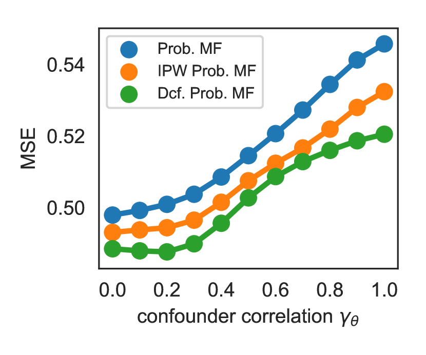
(a) Probabilistic MF

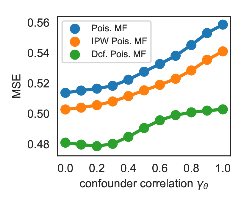
(b) Poisson MF

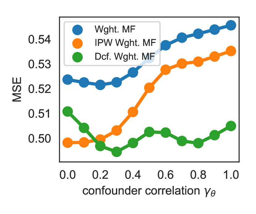
(c) Weighted MF

Figure 1: Varying confounder correlation $\gamma_{\theta}$ from 0.0 to 1.0 ($\gamma_{y}=3.0$). The rating predictions of the deconfounded recommender (green) is more robust to unobserved confounding than its classical counterpart (blue) and the existing causal approach, IPW MF (schnabel2016recommendations) (orange). (Lower is better.)

3.3 Case studies I: The deconfounded recommender on random test sets

We next study the deconfounded recommender on two real datasets: Yahoo! R3 (marlin2009collaborative) and coat shopping (schnabel2016recommendations). Both datasets are comprised of an observational training set and a random test set. The training set comes from users rating user-selected items; the random test set comes from the recommender system asking its users to rate randomly selected items. The latter enables us to evaluate how different recommendation models predict potential outcomes: what would the rating be if we make a user watch and rate a movie?

Datasets.  Yahoo! R3 (marlin2009collaborative) contains user-song ratings. The training set contains over 300K user-selected ratings from 15400 users on 1000 items. Its random test set contains 5400 users who were asked to rate 10 randomly chosen songs. The coat shopping dataset (schnabel2016recommendations) contains user-coat ratings. The training set contains 290 users. Each user supplies 24 user-selected ratings among 300 items. Its random test contains ratings for 16 randomly selected coat per user.

Evaluation metrics.  We use the recommenders for two types of prediction: weak generalization and strong generalization (marlin2004modeling). Weak generalization predicts preferences of existing users in the training set on their unseen movies. Strong generalization predicts preferences of new users—users not in the training set—on their unseen movies. Based on the predictions, we rank the items with nonzero ratings. To evaluate recommendation performance, we report three standard measures: ndcg, recall, and MSE. See Appendix D for formal definitions.

Experimental setup.  For each dataset, we randomly split 80/20 the training set into training/validation sets. We leave the random test set intact. Across all experiments, we use the validation set to select the best hyperparameters for the recommendation models. We choose the hyperparameters that yield the best validation log NDCG. The latent dimension is chosen from $\{1,2,5,10,20,50,100\}$.

The deconfounded recommender has two components: the treatment assignment model and the outcome model. We always use pf as the treatment assignment model. The hyperparameters of both models are chosen together based on the same validation set as above. The best hyperparameters are those that yield the best validation NDCG.

Results.  § 3.3 and 3.3 show the recommendation performance of the deconfounded recommender and its competitors. Across the three metrics and the two datasets, the deconfounded recommender outperforms its classical counterpart for both weak and strong generalization: it produces better item rankings and improves retrieval quality; its predicted ratings are also more accurate. The deconfounded recommender also outperforms the ipw matrix factorization (schnabel2016recommendations), which is the main existing approach that targets selection bias in recommendation systems. These results show that the deconfounded recommender produces more accurate predictions of user preferences by accommodating unobserved confounders in item exposures.

	Yahoo! R3				Coat
	NDCG	Recall@5	MSE		NDCG	Recall@5	MSE
Probabilistic MF [mnih2008probabilistic]	0.772	0.540	1.963		0.728	0.552	1.422
IPW Probabilistic MF [schnabel2016recommendations]	0.791	0.603	1.893		0.732	0.547	1.358
Deconfounded Probabilistic MF	0.819	0.640	1.768		0.743	0.569	1.341
1-8 Poisson MF [gopalan2015scalable]	0.789	0.564	1.539		0.713	0.451	1.657
IPW Poisson MF [schnabel2016recommendations]	0.792	0.564	1.513		0.693	0.458	1.631
Deconfounded Poisson MF	0.802	0.610	1.447		0.743	0.521	1.657
1-8 Weighted MF [hu2008collaborative]	0.820	0.639	2.047		0.738	0.560	1.658
IPW Weighted MF [schnabel2016recommendations]	0.804	0.592	1.845		0.681	0.554	1.612
Deconfounded Weighted MF	0.823	0.645	1.658		0.744	0.581	1.569

Table 1: Recommendation on random test sets for existing users (weak generalization). The deconfounded recommender improves recommendation over classical approaches and the existing causal approach (schnabel2016recommendations). (Higher is better for NDCG and Recall@5; lower is better for MSE.)

	Yahoo! R3				Coat
	NDCG	Recall@5	MSE		NDCG	Recall@5	MSE
Probabilistic MF [mnih2008probabilistic]	0.802	0.792	2.307		0.833	0.737	1.490
IPW Probabilistic MF [schnabel2016recommendations]	0.818	0.827	2.625		0.811	0.724	1.587
Deconfounded Probabilistic MF	0.824	0.829	2.244		0.847	0.808	1.540
1-8 Poisson MF [gopalan2015scalable]	0.765	0.752	1.913		0.764	0.671	1.889
IPW Poisson MF [schnabel2016recommendations]	0.769	0.761	1.876		0.769	0.678	1.817
Deconfounded Poisson MF	0.774	0.769	1.881		0.772	0.678	1.811
1-8 Weighted MF [hu2008collaborative]	0.809	0.793	1.904		0.850	0.814	2.859
IPW Weighted MF [schnabel2016recommendations]	0.786	0.788	1.883		0.837	0.800	2.477
Deconfounded Weighted MF	0.820	0.818	1.644		0.854	0.829	2.421

Table 2: Recommendation on random test sets for new users (strong generalization). The deconfounded recommender improves recommendation over classical approaches and the existing causal approach (schnabel2016recommendations). (Higher is better for NDCG and Recall@5; lower is better for MSE.)

3.4 Case studies II: The deconfounded recommender on regular test sets

We study the deconfounded recommender on two MovieLens datasets: ML100k and ML1M. These datasets only involve observational data; they do not contain randomized test sets. We focus on how well we predicts on all items, popular or unpopular.

Datasets.  The Movielens 100k dataset contains 100,000 ratings from 1,000 users on 1,700 movies. The Movielens 1M dataset contains 1 million ratings from 6,000 users on 4,000 movies.

Experimental setup and performance measures.  We employ the same experimental protocols for hyperparameter selection as before. For each dataset, we randomly split the training set into training/validation/test sets with 60/20/20 proportions. We measure the recommendation performance by the average per-item predictive accuracy, which equally treats popular and unpopular items; see § 3.1 for details.

Results.  § 3.4 presents the recommendation performance of the deconfounded recommender and their classical counterpart on average per-item MSEs and MAEs. Across the two metrics and two datasets, the deconfounded recommender leads to lower MSEs and MAEs on predictions over all items than classical approaches and the existing causal approach, IPW MF (schnabel2016recommendations). Instead of focusing on popular items, the deconfounded recommender targets accurate predictions on all items. Hence it improves the prediction quality across all items.

	Movielens 100K			Movielens 1M
	MSE	MAE		MSE	MAE
Probabilistic MF [mnih2008probabilistic]	2.926	1.425		2.774	1.321
IPW Probabilistic MF [schnabel2016recommendations]	2.609	1.275		2.714	1.303
Deconfounded Probabilistic MF	2.554	1.260		2.699	1.299
1-6 Poisson MF [gopalan2015scalable]	3.374	1.475		2.357	1.305
IPW Poisson MF [schnabel2016recommendations]	3.439	1.480		2.196	1.220
Deconfounded Poisson MF	3.268	1.454		2.325	1.295
1-6 Weighted MF [hu2008collaborative]	2.359	1.219		3.558	1.516
IPW Weighted MF [schnabel2016recommendations]	2.344	1.198		2.872	1.363
Deconfounded Weighted MF	2.101	1.138		2.864	1.360

Table 3: Average per-item predictive accuracy on heldout ratings. The deconfounded recommender leads to lower MSEs and MAEs on predictions over all items; it outperforms classical approaches and the existing causal approach (schnabel2016recommendations). (Lower is better.)

4 Discussion

We develop the deconfounded recommender, a strategy to use classical recommendation models for causal predictions: how would a user rate a recommended movie? The deconfounded recommender uses Poisson factorization to infer confounders in treatment assignments; it then augments common recommendation models to correct for confounding bias. The deconfounded recommender improves recommendation performance and rating predictions; it is also more robust to unobserved confounding in user exposures.

Supplementary Material

Appendix A Theoretical justification of the deconfounded recommender

The following theorem formalizes the theoretical justification of the deconfounded recommender.

Theorem 1.

If no confounders affect the exposure to only one of the items, and the number of items go to infinity, then the deconfounded recommender forms unbiased causal inference

$$E[Y_{ui}(a)]=E[E[Y_{ui}(A_{ui})\,|\,A_{ui}=a,\pi_{u}^{\top}\lambda_{i}]]\quad\text{ for all }u,i,$$ (9)

when $A_{ui}\sim\textrm{Poisson}(\pi_{u}^{\top}\lambda_{i})$ for some independent random vectors $\pi_{u}$’s and $\lambda_{i}$’s,

This theorem follows from Proposition 5 and Theorem 7 of (wang2018blessings) in addition to the fact that $\pi_{u}\mathchoice{\mathrel{\hbox to0.0pt{$\displaystyle\perp$\hss}\mkern 2.0mu{\displaystyle\perp}}}{\mathrel{\hbox to0.0pt{$\textstyle\perp$\hss}\mkern 2.0mu{\textstyle\perp}}}{\mathrel{\hbox to0.0pt{$\scriptstyle\perp$\hss}\mkern 2.0mu{\scriptstyle\perp}}}{\mathrel{\hbox to0.0pt{$\scriptscriptstyle\perp$\hss}\mkern 2.0mu{\scriptscriptstyle\perp}}}\mathbb{1}\{A_{ui}=a\}\,|\,p(A_{ui}=a\,|\,\pi_{u}^{\top}\lambda_{i})$ (hirano2004propensity). Specifically, Proposition 5 of (wang2018blessings) asserts the ignorability of the substitute confounder; Theorem 7 of (wang2018blessings) establishes causal identification of the deconfounder on the intervention of subsets of the causes. The deconfounded recommender fits into this setting because $Y_{ui}(a)$ is a counterfactual quantity involving only one item (cause), i.e. the exposure to item $i$.

Proposition 5 and Theorem 7 of wang2018blessings implies

$$E[Y_{ui}(a)]=E[E[Y_{ui}(A_{ui})\,|\,A_{ui}=a,\pi_{u}]]\quad\text{ for all }u,i.$$

Therefore, we have

$$E[Y_{ui}(a)] =E[E[Y_{ui}(A_{ui})\,|\,A_{ui}=a,\pi_{u}]]$$

$$=E[E[Y_{ui}(A_{ui})\,|\,\mathbb{1}\{A_{ui}=a\},\pi_{u}]]$$

$$=E[E[E[Y_{ui}(A_{ui})\,|\,\mathbb{1}\{A_{ui}=a\},\pi_{u},p(A_{ui}=a\,|\,\pi_{u}^{\top}\lambda_{i})]]]$$

$$=E[E[E[Y_{ui}(A_{ui})\,|\,\mathbb{1}\{A_{ui}=a\},p(A_{ui}=a\,|\,\pi_{u}^{\top}\lambda_{i})]]]$$

$$=E[E[E[Y_{ui}(A_{ui})\,|\,\mathbb{1}\{A_{ui}=a\},\pi_{u}^{\top}\lambda_{i}]]]$$

$$=E[E[E[Y_{ui}(A_{ui})\,|\,A_{ui}=a,\pi_{u}^{\top}\lambda_{i}]]]$$

The first three equalities are due to basic probability facts. The fourth equality is due to $\pi_{u}\mathchoice{\mathrel{\hbox to0.0pt{$\displaystyle\perp$\hss}\mkern 2.0mu{\displaystyle\perp}}}{\mathrel{\hbox to0.0pt{$\textstyle\perp$\hss}\mkern 2.0mu{\textstyle\perp}}}{\mathrel{\hbox to0.0pt{$\scriptstyle\perp$\hss}\mkern 2.0mu{\scriptstyle\perp}}}{\mathrel{\hbox to0.0pt{$\scriptscriptstyle\perp$\hss}\mkern 2.0mu{\scriptscriptstyle\perp}}}\mathbb{1}\{A_{ui}=a\}\,|\,p(A_{ui}=a\,|\,\pi_{u}^{\top}\lambda_{i})$ (hirano2004propensity). The fifth equality is due to $A_{ui}\sim\textrm{Poisson}(\pi_{u}^{\top}\lambda_{i})$. The last equality is again due to basic probability facts.

Appendix B Beyond probabilistic matrix factorization

Focusing on pf as the exposure model, we extend the deconfounded recommender to general outcome models.

We start with a general form of matrix factorization,

$$y_{ui}(a)\sim p(\cdot\,|\,m(\theta_{u}^{\top}\beta_{i},a),v(\theta_{u}^{\top}\beta_{i},a)),$$ (10)

where $m(\theta_{u}^{\top}\beta_{i},a)$ characterizes the mean and $v(\theta_{u}^{\top}\beta_{i},a)$ the variance of the ratings $y_{ui}(a)$. This form encompasses many factorization models. Probabilistic matrix factorization (mnih2008probabilistic) is

$$m(\theta_{u}^{\top}\beta_{i},a)=a\cdot\theta_{u}^{\top}\beta_{i},\quad v(\theta_{u}^{\top}\beta_{i},a)=\sigma^{2},$$

and $p(\cdot)$ is the Gaussian distribution. Weighted matrix factorization (hu2008collaborative) also involves a Gaussian $p$, but its variance changes based on whether a user has seen the movie:

$$m(\theta_{u}^{\top}\beta_{i},a)=\theta_{u}^{\top}\beta_{i},\quad v(\theta_{u}^{\top}\beta_{i},a)=\sigma^{2}_{a},$$

where $\sigma_{0}^{2}=\alpha\sigma_{1}^{2}$. This model leads us to downweight the zeros; we are less confident about the zero ratings. Poisson matrix factorization as an outcome model (gopalan2015scalable) only takes in a mean parameter

$$m(\theta_{u}^{\top}\beta_{i},a)=\theta_{u}^{\top}\beta_{i}$$

and set $p(\cdot)$ to be the Poisson distribution.

With the general matrix factorization of Eq. 10, the deconfounded recommender fits an augmented outcome model $M_{Y}$. This outcome model $M_{Y}$ includes the substitute confounder as a covariate,

$$y_{ui}(a)\sim p(\cdot\,|\,m(\theta_{u}^{\top}\beta_{i},a)+\gamma_{u}\hat{a}_{ui}+\beta_{0},v(\theta_{u}^{\top}\beta_{i},a)).$$ (11)

Notice the parameter $\gamma_{u}$ is a user-specific coefficient; for each user, it characterizes how much the substitute confounder $\hat{a}$ contributes to the ratings. Note the deconfounded recommender also includes an intercept $\beta_{0}$. These deconfounded outcome model can be fit by maximum a posteriori estimation.

It solves

$$\textstyle\hat{\theta}_{u},\hat{\beta}_{i},\hat{\gamma}_{u},\hat{\beta}_{0}$$

$$= \operatorname*{arg\,max}\sum_{u=1}^{U}\sum_{i=1}^{I}\log p(y_{ui};m(\theta_{u}^{\top}\beta_{i},a_{ui})+\gamma_{u}\hat{a}_{ui}+\beta_{0},$$

$$v(\theta_{u}^{\top}\beta_{i},a_{ui}))\textstyle+\sum_{u=1}^{U}\log p(\theta_{u})+\sum_{i=1}^{I}\log p(\beta_{i})$$

$$+\sum_{u=1}^{U}\log p(\gamma_{u})+\log p(\beta_{0}),$$

where $p(\theta_{u})$, $p(\beta_{i})$, $p(\gamma_{u})$, and $p(\beta_{0})$ are priors of the latent variables.

To form recommendations, the deconfounded recommender predicts all of the potential ratings, $y_{ui}(1)$. For an existing user $u$, it computes the potential ratings from the fitted outcome model,

$$\hat{y}_{ui}(1)=m(\hat{\theta}_{u}^{\top}\hat{\beta}_{i},1)+\hat{\gamma}_{u}\cdot\hat{a}_{ui}+\hat{\beta}_{0}.$$ (12)

For a new user $u^{\prime}$ with only a few ratings, it fixes the item vectors $\lambda_{i}$ and $\beta_{i}$, and compute user vectors for the new user: it fits $\pi_{u^{\prime}}$, $\theta_{u^{\prime}}$, and $\gamma_{u^{\prime}}$ from the exposure and the ratings of this new user $u^{\prime}$. It finally computes the prediction,

$$\hat{y}_{u^{\prime}i}(1)=m(\hat{\theta}_{u^{\prime}}^{\top}\hat{\beta}_{i},1)+\hat{\gamma}_{u^{\prime}}\cdot\hat{\pi}_{u^{\prime}}^{\top}\lambda_{i}+\hat{\beta}_{0}.$$ (13)

The deconfounded recommender ranks all the items for each user based on $\hat{y}_{ui}(1),i=1,\ldots,I$, and recommends highly ranked items.

Appendix C Detailed simulation results

Figures 2 and 1 explore how an unobserved confounder high correlated with exposures can affect rating predictions and ranking quality of recommendation algorithms.

Figures 3 and 4 explore how an unobserved confounder high correlated with the rating outcome can affect rating predictions and ranking quality of recommendation algorithms.

In both simulations, we find that the deconfounded recommender is more robust to unobserved confounding; it leads to smaller MSEs in rating prediction and higher NDCGs in recommendation than its classical counterparts (Probabilistic/Poisson/Weighted MF) and the existing causal approach (ipw MF (schnabel2016recommendations)).

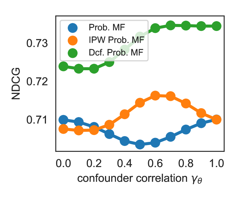
(a) Probabilistic MF

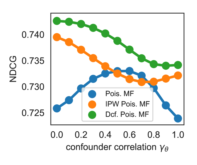
(b) Poisson MF

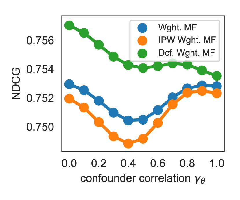
(c) Weighted MF

Figure 2: Varying confounding correlation $\gamma_{\theta}$ from 0.0 to 1.0 ($\gamma_{y}=3.0$). The ranking quality of the deconfounded recommender (green) is more robust to unobserved confounding than its classical counterpart (blue) and the existing causal approach (orange) (schnabel2016recommendations). Higher is better. (Results averaged over 10 runs.)

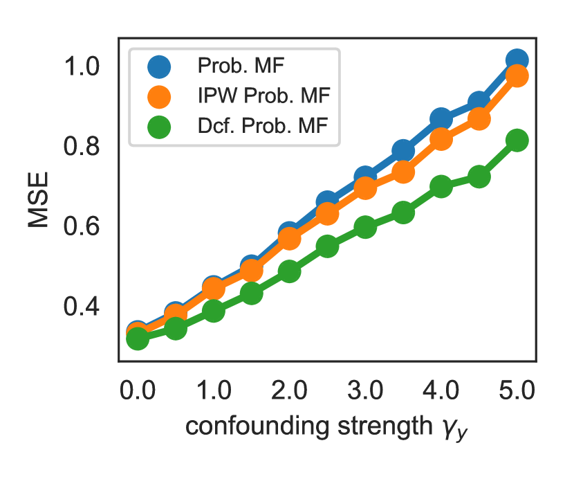
(a) Probabilistic MF

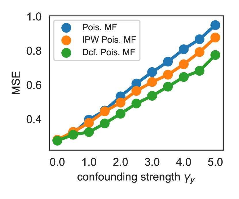
(b) Poisson MF

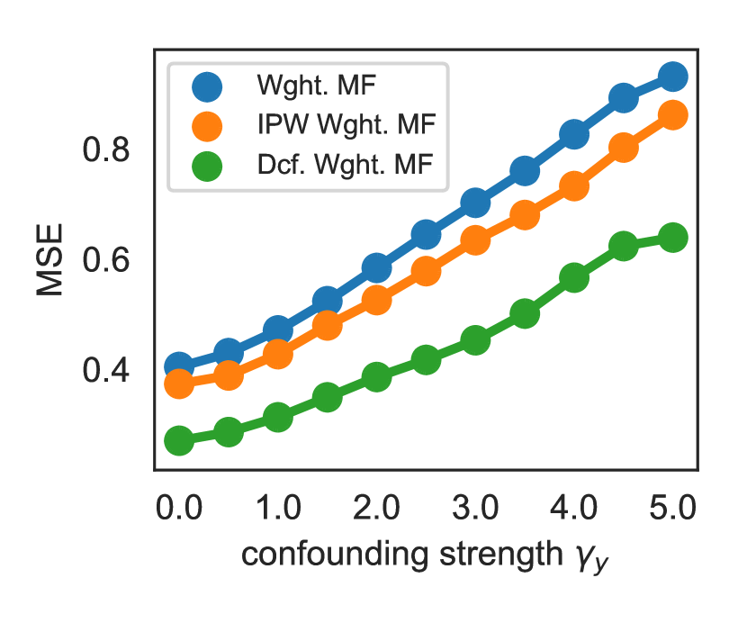
(c) Weighted MF

Figure 3: Varying confounding strength $\gamma_{y}$ from 0.0 to 5.0 ($\gamma_{\theta}=0.6$). The rating predictions of the deconfounded recommender (green) is more robust to unobserved confounding than its classical counterpart (blue) and the existing causal approach (orange) (schnabel2016recommendations). Lower is better. (Results averaged over 10 runs.)

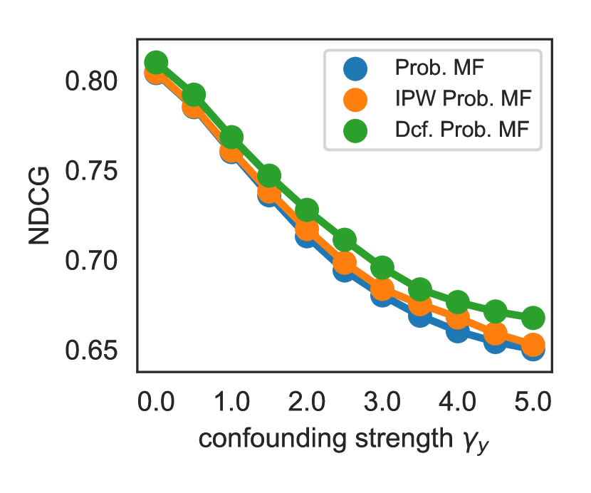
(a) Probabilistic MF

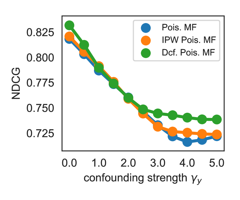
(b) Poisson MF

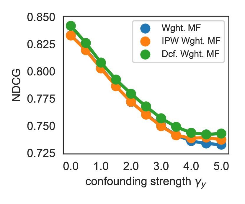
(c) Weighted MF

Figure 4: Varying confounding strength $\gamma_{y}$ from 0.0 to 5.0 ($\gamma_{\theta}=0.6$). The ranking quality of the deconfounded recommender (green) is more robust to unobserved confounding than its classical counterpart (blue) and the existing causal approach (orange) (schnabel2016recommendations). Higher is better. (Results averaged over 10 runs.)

Appendix D Performance measures

Denote $rank(u,i)$ as the rank of item $i$ in user $u$’s predicted list; let $y_{u}^{\mathrm{test}}$ as the set of relevant items in the test set of user $u$.

• ndcg measures ranking quality:

  $$DCG=\frac{1}{U}\sum_{u=1}^{U}\sum_{i=1}^{L}\frac{2^{\mathrm{rel}_{ui}-1}}{\log_{2}(i+1)},\quad NDCG=\frac{DCG}{IDCG},$$

  where $L$ is the number of items in the test set of user $u$, the relevance $\mathrm{rel}_{ui}$ is set as the rating of user $u$ on item $i$, and $IDCG$ is a normalizer that ensures $NDCG$ sits between 0 and 1.

• Recall@k. Recall@k evaluates how many relevant items are selected:

  $$\textrm{Recall@k}=\frac{1}{U}\sum_{u=1}^{U}\sum_{i\in y_{u}^{\mathrm{test}}}\frac{\mathbb{1}\{rank(u,i)\leq k\}}{\min(k,|y_{u}^{\mathrm{test}}|)}.$$

• MSE. MSE evaluates how far the predicted ratings are away from the true rating:

  $$\textrm{MSE}=\frac{1}{|(u,i)\in y^{\mathrm{test}}|}\sum_{(u,i)\in y^{\mathrm{test}}}(\hat{y}_{ui}-y_{ui})^{2}.$$

Appendix E Experimental Details

For weighted matrix factorization, we set weights of the observation by $c_{ui}=1+\alpha y_{ui}$ where $\alpha=40$ following (hu2008collaborative).

For Gaussian latent variables in probabilistic matrix factorization, we use priors $\mathcal{N}(0,1)$ or $\mathcal{N}(0,0.1^{2})$.

For Gamma latent variables in pf, we use prior $\textrm{Gamma}(0.3,0.3).$

For inverse propensity weighting (ipw) matrix factorization (schnabel2016recommendations), we following Section 6.2 of schnabel2016recommendations. We set the propensity $p_{ui}$ to be $p_{ui}=k$ for ratings $y_{ui}\geq 4$ and $p_{ui}=k\alpha^{4-y_{ui}}$ for ratings $y_{ui}<4$, where $\alpha=0.25$ and $k$ is set so that $\frac{1}{U\cdot I}\sum_{u=1}^{U}\sum_{i=1}^{I}p_{ui}=0.05$. We then perform inverse propensity weighting (ipw) matrix factorization with the estimated propensities.