Naturality of the Contact Invariant in Monopole Floer Homology Under Strong Symplectic Cobordisms

Abstract.

The contact invariant is an element in the monopole Floer homology groups of an oriented closed three manifold canonically associated to a given contact structure. A non-vanishing contact invariant implies that the original contact structure is tight, so understanding its behavior under symplectic cobordisms is of interest if one wants to further exploit this property.

By extending the gluing argument of Mrowka and Rollin to the case of a manifold with a cylindrical end, we will show that the contact invariant behaves naturally under a strong symplectic cobordism.

As quick applications of the naturality property, we give alternative proofs for the vanishing of the contact invariant in the case of an overtwisted contact structure, its non-vanishing in the case of strongly fillable contact structures and its vanishing in the reduced part of the monopole Floer homology group in the case of a planar contact structure. We also prove that a strong filling of a contact manifold which is an $L$-space must be negative definite.

1. Stating the Result and Some Applications

Monopole Floer Homology associates to a closed, oriented, connected 3-manifold $Y$ three abelian groups $\savestack{\tmpbox}{\stretchto{\scaleto{\scalerel*[\widthof{HM}]{\kern-0.6pt\bigwedge\kern-0.6pt}{\rule[-505.89pt]{4.30554pt}{505.89pt}}}{}}{0.5ex}}\stackon[1pt]{HM}{\scalebox{-1.0}{\tmpbox}}_{\bullet}(Y)$ , $\widehat{HM}_{\bullet}(Y)$, $\overline{HM}_{\bullet}(Y)$, pronounced $HM$-to, $HM$-from and $HM$-bar respectively. They admit a direct sum decomposition over spin-c structures of $Y$, in the sense that

$$\savestack{\tmpbox}{\stretchto{\scaleto{\scalerel*[\widthof{HM}]{\kern-0.6pt\bigwedge\kern-0.6pt}{\rule[-505.89pt]{4.30554pt}{505.89pt}}}{}}{0.5ex}}\stackon[1pt]{HM}{\scalebox{-1.0}{\tmpbox}}_{\bullet}(Y)=\bigoplus_{\mathfrak{s}}\savestack{\tmpbox}{\stretchto{\scaleto{\scalerel*[\widthof{HM}]{\kern-0.6pt\bigwedge\kern-0.6pt}{\rule[-505.89pt]{4.30554pt}{505.89pt}}}{}}{0.5ex}}\stackon[1pt]{HM}{\scalebox{-1.0}{\tmpbox}}_{\bullet}(Y,\mathfrak{s}$$

$$\widehat{HM}_{\bullet}(Y)=\bigoplus_{\mathfrak{s}}\widehat{HM}_{\bullet}(Y,\mathfrak{s})$$

$$\overline{HM}_{\bullet}(Y)=\bigoplus_{\mathfrak{s}}\overline{HM}_{\bullet}(Y,\mathfrak{s})$$

In fact, the previous decomposition is finite [26, Proposition 3.1.1]. The chain complexes whose homology are the previous groups are built using solutions of a perturbed version of the three dimensional Seiberg-Witten equations, which are at the same time critical points of a perturbed Chern-Simons-Dirac functional [26, Section 4]. There are three different types of solutions (the boundary stable, boundary unstable and irreducible solutions) and each group uses two of the three types in their corresponding construction.

Now suppose that $Y$ is equipped with a co-orientable contact structure $\xi$ compatible with the orientation of the manifold. In practice this means that there exists a globally defined one form $\theta$ on $Y$ for which $\xi=\ker\theta$ and $\theta\wedge d\theta$ is positive everywhere [17, Lemma 1.1.1]. As we will review momentarily, $\xi$ determines a spin-c structure $\mathfrak{s}_{\xi}$ and one can exploit the additional structure provided by $\xi$ in order to construct an element $\mathbf{c}(\xi)\in\savestack{\tmpbox}{\stretchto{\scaleto{\scalerel*[\widthof{HM}]{\kern-0.6pt\bigwedge\kern-0.6pt}{\rule[-505.89pt]{4.30554pt}{505.89pt}}}{}}{0.5ex}}\stackon[1pt]{HM}{\scalebox{-1.0}{\tmpbox}}_{\bullet}(-Y,\mathfrak{s}_{\xi})$ known as the contact invariant of $(Y,\xi)$.

It is important to observe that $\mathbf{c}(\xi)$ belongs to the monopole Floer homology groups of the manifold $-Y$, that is, $Y$ with the opposite orientation. This is because the contact invariant $\mathbf{c}(\xi)$ should actually be regarded as a cohomology element $\mathbf{c}(\xi)\in\widehat{HM}^{\bullet}(Y,\mathfrak{s}_{\xi})$, and there is a natural isomorphism between $\widehat{HM}^{\bullet}(Y,\mathfrak{s}_{\xi})$ and $\savestack{\tmpbox}{\stretchto{\scaleto{\scalerel*[\widthof{HM}]{\kern-0.6pt\bigwedge\kern-0.6pt}{\rule[-505.89pt]{4.30554pt}{505.89pt}}}{}}{0.5ex}}\stackon[1pt]{HM}{\scalebox{-1.0}{\tmpbox}}_{\bullet}(-Y,\mathfrak{s}_{\xi})$ [26, Section 22.5]. However, we will work with the homology version of the contact invariant since most of the formulas in [26] are given explicitly for the homology groups.

Monopole Floer homology also has TFQT-like features, which concretely means that given a cobordism $W:Y\rightarrow Y^{\prime}$ between two three manifolds, there are group homomorphisms between the corresponding homology groups

$$\savestack{\tmpbox}{\stretchto{\scaleto{\scalerel*[\widthof{HM}]{\kern-0.6pt\bigwedge\kern-0.6pt}{\rule[-505.89pt]{4.30554pt}{505.89pt}}}{}}{0.5ex}}\stackon[1pt]{HM}{\scalebox{-1.0}{\tmpbox}}_{\bullet}(W,\mathfrak{s}_{W}):\savestack{\tmpbox}{\stretchto{\scaleto{\scalerel*[\widthof{HM}]{\kern-0.6pt\bigwedge\kern-0.6pt}{\rule[-505.89pt]{4.30554pt}{505.89pt}}}{}}{0.5ex}}\stackon[1pt]{HM}{\scalebox{-1.0}{\tmpbox}}_{\bullet}(Y,\mathfrak{s}_{Y})\rightarrow\savestack{\tmpbox}{\stretchto{\scaleto{\scalerel*[\widthof{HM}]{\kern-0.6pt\bigwedge\kern-0.6pt}{\rule[-505.89pt]{4.30554pt}{505.89pt}}}{}}{0.5ex}}\stackon[1pt]{HM}{\scalebox{-1.0}{\tmpbox}}_{\bullet}(Y^{\prime},\mathfrak{s}_{Y^{\prime}}$$

$$\widehat{HM}_{\bullet}(W,\mathfrak{s}_{W}):\widehat{HM}_{\bullet}(Y,\mathfrak{s}_{Y})\rightarrow\widehat{HM}_{\bullet}(Y^{\prime},\mathfrak{s}_{Y^{\prime}})$$

$$\overline{HM}_{\bullet}(W,\mathfrak{s}_{W}):\overline{HM}_{\bullet}(Y,\mathfrak{s}_{Y})\rightarrow\overline{HM}_{\bullet}(Y^{\prime},\mathfrak{s}_{Y^{\prime}})$$

Here $\mathfrak{s}_{W}$ denotes a spin-c structure which restricts in an appropriate sense to the given spin-c structures on $Y$ and $Y^{\prime}$. Just as in the contact case, if $(W,\omega):(Y,\xi)\rightarrow(Y^{\prime},\xi^{\prime})$ is equipped with a symplectic form $\omega$, it determines a spin-c structure $\mathfrak{s}_{\omega}$ , and so it makes sense to ask the naturality question, that is, whether or not

(1) $$\savestack{\tmpbox}{\stretchto{\scaleto{\scalerel*[\widthof{HM}]{\kern-0.6pt\bigwedge\kern-0.6pt}{\rule[-505.89pt]{4.30554pt}{505.89pt}}}{}}{0.5ex}}\stackon[1pt]{HM}{\scalebox{-1.0}{\tmpbox}}_{\bullet}(W^{\dagger},\mathfrak{s}_{\omega})\mathbf{c}(\xi^{\prime})\overset{?}{=}\mathbf{c}(\xi)$$

where $W^{\dagger}:-Y^{\prime}\rightarrow-Y$ denotes the cobordism turned “upside-down”. The main result of this work is that the answer to the previous question is positive in the case of a strong symplectic cobordism:

Theorem 1.

Let $(W,\omega):(Y,\xi)\rightarrow(Y^{\prime},\xi^{\prime})$ be a strong symplectic cobordism between two contact manifolds $(Y,\xi)$ and $(Y^{\prime},\xi^{\prime})$. Then

$$\savestack{\tmpbox}{\stretchto{\scaleto{\scalerel*[\widthof{HM}]{\kern-0.6pt\bigwedge\kern-0.6pt}{\rule[-505.89pt]{4.30554pt}{505.89pt}}}{}}{0.5ex}}\stackon[1pt]{HM}{\scalebox{-1.0}{\tmpbox}}_{\bullet}(W^{\dagger},\mathfrak{s}_{\omega})\mathbf{c}(\xi^{\prime};\mathbb{F}_{2})=\mathbf{c}(\xi;\mathbb{F}_{2})$$

Here we have added an $\mathbb{F}_{2}$ to our notation of the contact invariant to emphasize that we are using the coefficient field $\mathbb{F}=\mathbb{Z}/2$ so that we can ignore orientation issues for the moduli spaces. However, throughout the paper we will drop the $\mathbb{F}_{2}$ from our notation for simplicity. Clearly one can also ask whether or not one there is an analogous statement in the case of integer coefficients. Unfortunately, Theorem $H$ in [23] shows that there is no canonical choice of sign in the definition of the contact invariant, so the best naturality statement one could hope for in this case is one given up to a sign.

At this point it is important to specify that our notion of a strong symplectic cobordism is that of a symplectic cobordism for which the symplectic form is given in collar neighborhoods of the concave and convex boundaries by symplectizations of the corresponding contact structures.

To give some context we should point out that this theorem appears stated as Theorem 2.4 in [40], though the reference given is a paper by Mrowka and Rollin in preparation that was never published. Also, as will be discussed later in this paper the “special” condition imposed on the cobordism in [40] and [32] can be removed.

One can also ask what is known in the twin versions of monopole Floer homology, namely, embedded contact homology and Heegaard Floer homology. It is not by any means obvious that the corresponding homology groups from Heegaard Floer and ECH are isomorphic to the ones coming from monopole Floer homology and the proof can be found in [3, 4, 5, 6, 7, 49, 50, 48, 43, 44, 45, 46, 47]. Also, the corresponding contact invariants in each version are isomorphic to each other.

In Heegaard Floer homology naturality holds (for example) if $(Y^{\prime},\xi^{\prime})$ is obtained from $(Y,\xi)$ by Legendrian surgery along a Legendrian knot $L$ [29, Theorem 2.3]. This is an interesting case because a 1-handle surgery, or a 2-handle surgery along a Legendrian knot $K$ with framing $-1$ relative to the canonical framing gives rise to a strong symplectic cobordism. On the ECH side the contact invariant is known to be well behaved with respect to weakly exact symplectic cobordisms [22, Remark 1.11]. Moreover, Michael Hutchings has communicated to the author that he can improve this result to the case of a strong symplectic cobordism, with the additional advantage that the contact manifolds can be disconnected [20].

As we will see, the contact invariant with mod-2 coefficients is a useful tool for understanding contact structures and our naturality result is good enough to find properties of this invariant, though the properties we discuss in this work were previously proven by other means. Before we mention these applications, however, we will give some brief history that puts into perspective the construction of the contact invariant and why the following results were natural things to look for.

In [25] Kronheimer and Mrowka used the contact structure of $Y$ to extend the definition of the Seiberg-Witten invariants to the case of a compact oriented four manifold $X$ bounding it.

More precisely, one considers the non-compact four manifold $X^{+}=X\cup_{Y}([1,\infty)\times Y)$, where $[1,\infty)\times Y$ is given the structure of an almost Kähler cone using a symplectization $\omega$ of a contact form $\theta$ defining $\xi$. In particular, the symplectic form induced by $\theta$ determines a canonical spin-c structure $\mathfrak{s}_{\omega}$ on $[1,\infty)\times Y$ , which we can think of as a complex vector bundle $S=S^{+}\oplus S^{-}$ together with a Clifford multiplication $\rho:T^{*}\left([1,\infty)\times Y\right)\rightarrow\hom_{\mathbb{C}}(S,S)$ satisfying certain conditions.

The canonical spin-c structure $\mathfrak{s}_{\omega}$ carries a canonical section $\varPhi_{0}$ of $S^{+}$ together with a canonical spin-c connection $A_{0}$ on the spinor bundle. Kronheimer and Mrowka then study solutions of the Seiberg Witten equations on $X^{+}$ which are asymptotic to $(A_{0},\varPhi_{0})$ on the conical end. These solutions end up having uniform exponential decay with respect to the canonical configuration $(A_{0},\varPhi_{0})$ (Proposition 3.15 in [25] or Propositions 5.7 and 5.10 in [54] for a similar situation), which means that the Seiberg Witten equations on $X^{+}$ behave very similar to how they would if the manifold were compact, more specifically, the moduli spaces of gauge equivalence classes of such solutions are compact. This allows as in the closed manifold case to define a map

$$SW_{(X,\xi)}:\text{Spin}^{c}(X,\xi)\rightarrow\mathbb{Z}$$

where $\text{Spin}^{c}(X,\xi)$ denotes the set of isomorphism classes of relative spin-c structures on $X$ that restrict to the spin-c structure $\mathfrak{s}_{\xi}$ on $Y$ determined by the contact structure $\xi$. This map can be used to detect properties of contact structures on three manifolds. For example, Theorem 1.3 in [25] shows that for any closed three manifold $Y$ there are only finitely many homotopy classes of 2-plane fields which are realized as semi-fillable contact structures. In section 1.3 of the same paper Kronheimer and Mrowka mention as well that if $(X,\xi)$ is a 4-manifold with an overtwisted contact structure on its boundary, then $SW_{(X,\xi)}$ vanishes identically.

The latter result is Corollary $B$ in a different paper [32] by Mrowka and Rollin, where they analyzed how the map $SW_{(X,\xi)}$ behaves under a symplectic cobordism $(W,\omega):(Y,\xi)\rightarrow(Y^{\prime},\xi^{\prime})$ which they called a special symplectic cobordism [32, Page 4]. Theorem D in [32] shows that

(2) $$SW_{(X,\xi)}=\pm SW_{(X\cup W,\xi^{\prime})}\circ\jmath$$

where $\jmath:\text{Spin}^{c}(X,\xi)\rightarrow\text{Spin}^{c}(X\cup W,\xi^{\prime})$ is a canonical map that extends the spin-c structure of $X$ across the cobordism $W$. With respect to $\mathbb{Z}/2\mathbb{Z}$ coefficients, the previous theorem can be interpreted as saying that the mod 2 Seiberg-Witten invariants are the same.

In order to detect more properties of the contact structure, we need to use the machinery of Monopole Floer Homology, whose canonical reference is [26].

As first defined in section 6.3 of [24] , one constructs the contact invariant $\mathbf{c}(\xi)\in\savestack{\tmpbox}{\stretchto{\scaleto{\scalerel*[\widthof{HM}]{\kern-0.6pt\bigwedge\kern-0.6pt}{\rule[-505.89pt]{4.30554pt}{505.89pt}}}{}}{0.5ex}}\stackon[1pt]{HM}{\scalebox{-1.0}{\tmpbox}}_{\bullet}(-Y,\mathfrak{s}_{\xi})$ by studying the Seiberg Witten equations on $(\mathbb{R}^{+}\times-Y)\cup([1,\infty)\times Y)$ which are asymptotic on the symplectic cone to the canonical configuration $(A_{0},\varPhi_{0})$ mentioned before and asymptotic on the half-cylinder to a solution of the (perturbed) three dimensional Seiberg-Witten equations. We will give more details about this construction in the next section. However, it should be clear that based on the analogy with the numerical Seiberg-Witten invariants $SW_{(X,\xi)}$, one would expect the naturality property (our main theorem 1) as well as the vanishing of the contact invariant for an overtwisted structure. It is the latter which we now indicate how to prove.

Corollary 2.

Let $(Y,\xi)$ be an overtwisted contact 3 manifold. Then the contact invariant of $\xi$ vanishes, that is, $\mathbf{c}(\xi)=0$.

Proof.

First we show that the 3-sphere $S^{3}$ admits an overtwisted structure $\xi_{ot}$ for which $\mathbf{c}(\xi_{ot})=0$. For this we will use Eliashberg’s theorem [12, Theorem 1.6.1] on the existence of an overtwisted contact structure in every homotopy class of oriented plane field, and the fact that the Floer groups of any three manifold $Y$ are graded by the set of homotopy classes of oriented plane fields [26, Section 3.1].

Thanks to Proposition 3.3.1 in [26], which describes the Floer homology groups of $S^{3}$, we can find a homotopy class of plane field $[\xi]$ for which $\savestack{\tmpbox}{\stretchto{\scaleto{\scalerel*[\widthof{HM}]{\kern-0.6pt\bigwedge\kern-0.6pt}{\rule[-505.89pt]{4.30554pt}{505.89pt}}}{}}{0.5ex}}\stackon[1pt]{HM}{\scalebox{-1.0}{\tmpbox}}_{[\xi]}(S^{3})=0$. Notice that in this case we are not specifying the spin-c structure because $S^{3}$ has only one up to isomorphism. By Eliashberg’s theorem we can choose an overtwisted structure $\xi_{ot}$ in the homotopy class $[\xi]$. Now, $\mathbf{c}(\xi_{ot})$ is supported in $\savestack{\tmpbox}{\stretchto{\scaleto{\scalerel*[\widthof{HM}]{\kern-0.6pt\bigwedge\kern-0.6pt}{\rule[-505.89pt]{4.30554pt}{505.89pt}}}{}}{0.5ex}}\stackon[1pt]{HM}{\scalebox{-1.0}{\tmpbox}}_{[\xi]}(-S^{3})\simeq\savestack{\tmpbox}{\stretchto{\scaleto{\scalerel*[\widthof{HM}]{\kern-0.6pt\bigwedge\kern-0.6pt}{\rule[-505.89pt]{4.30554pt}{505.89pt}}}{}}{0.5ex}}\stackon[1pt]{HM}{\scalebox{-1.0}{\tmpbox}}_{[\xi]}(S^{3})=0$ and so it will automatically vanish, i.e, $\mathbf{c}(\xi_{ot})=0$.

Now, if $(Y,\xi)$ is an arbitrary overtwisted contact 3 manifold, using Theorem 1.2 in [14], we can find a Stein cobordism $(W,\omega):(Y,\xi)\rightarrow(S^{3},\xi_{ot})$. Such cobordisms are in fact strong cobordisms so we can conclude that

$$\mathbf{c}(\xi)=\savestack{\tmpbox}{\stretchto{\scaleto{\scalerel*[\widthof{HM}]{\kern-0.6pt\bigwedge\kern-0.6pt}{\rule[-505.89pt]{4.30554pt}{505.89pt}}}{}}{0.5ex}}\stackon[1pt]{HM}{\scalebox{-1.0}{\tmpbox}}_{\bullet}(W^{\dagger},\mathfrak{s}_{\omega})\mathbf{c}(\xi_{ot})=\savestack{\tmpbox}{\stretchto{\scaleto{\scalerel*[\widthof{HM}]{\kern-0.6pt\bigwedge\kern-0.6pt}{\rule[-505.89pt]{4.30554pt}{505.89pt}}}{}}{0.5ex}}\stackon[1pt]{HM}{\scalebox{-1.0}{\tmpbox}}_{\bullet}(W^{\dagger},\mathfrak{s}_{\omega})(0)=0$$

and therefore $\mathbf{c}(\xi)$ vanishes. ∎

Remark 3.

For a proof that does not use the naturality property see Theorem 4.2 in [42]. The vanishing of the contact invariant for overtwisted contact structures is also known on the Heegaard Floer side [38, Theorem 1.4]. For a proof on the ECH side see Michael Hutchings’ blog [21]. In fact, in the case of ECH one can show that the contact invariant vanishes in the case of planar torsion [51]. The same is also true in the Monopole Floer Homology side thanks to our naturality result and Theorem 1 in [52].

Corollary 4.

Let $(X,\omega)$ be a strong filling of $(Y,\xi)$. Then the contact invariant of $\xi$ is non-vanishing, that is, $\mathbf{c}(\xi)\neq 0$.

Proof.

By Darboux’s theorem we can remove a standard small ball $B$ of $X$ to obtain a strong cobordism $(W,\omega):(S^{3},\xi_{tight})\rightarrow(Y,\xi)$. Naturality says that $\mathbf{c}(\xi_{tight})=\savestack{\tmpbox}{\stretchto{\scaleto{\scalerel*[\widthof{HM}]{\kern-0.6pt\bigwedge\kern-0.6pt}{\rule[-505.89pt]{4.30554pt}{505.89pt}}}{}}{0.5ex}}\stackon[1pt]{HM}{\scalebox{-1.0}{\tmpbox}}_{\bullet}(W^{\dagger},\mathfrak{s}_{\omega})\mathbf{c}(\xi)$ but the left hand side is non-vanishing and so we conclude that $\mathbf{c}(\xi)$ is non-vanishing as well. ∎

Remark 5.

The Heegaard Floer version of this fact appears as Theorem 2.13 in [18]. That same paper contains an example of a weak filling where the contact invariant vanishes.

To explain the next corollary we do a quick review of some of the properties of the monopole Floer homology groups. Formally they behave like the ordinary homology groups $H_{*}(Z)$, $H_{*}(Z,A)$ and $H_{*}(A)$ for a pair of spaces in that they are related by a long exact sequence [26, Section 3.1]

(3) $$\cdots\overset{i_{*}}{\longrightarrow}\savestack{\tmpbox}{\stretchto{\scaleto{\scalerel*[\widthof{HM}]{\kern-0.6pt\bigwedge\kern-0.6pt}{\rule[-505.89pt]{4.30554pt}{505.89pt}}}{}}{0.5ex}}\stackon[1pt]{HM}{\scalebox{-1.0}{\tmpbox}}_{\bullet}(Y,\mathfrak{s})\overset{j_{*}}{\longrightarrow}\widehat{HM}_{\bullet}(Y,\mathfrak{s})\overset{p_{*}}{\longrightarrow}\overline{HM}_{\bullet}(Y,\mathfrak{s})\overset{i_{*}}{\longrightarrow}\savestack{\tmpbox}{\stretchto{\scaleto{\scalerel*[\widthof{HM}]{\kern-0.6pt\bigwedge\kern-0.6pt}{\rule[-505.89pt]{4.30554pt}{505.89pt}}}{}}{0.5ex}}\stackon[1pt]{HM}{\scalebox{-1.0}{\tmpbox}}_{\bullet}(Y,\mathfrak{s})\overset{j_{*}}{\longrightarrow}\cdots$$

An important subgroup of $\widehat{HM}_{\bullet}(Y,\mathfrak{s})$ is the image of $j_{*}:\savestack{\tmpbox}{\stretchto{\scaleto{\scalerel*[\widthof{HM}]{\kern-0.6pt\bigwedge\kern-0.6pt}{\rule[-505.89pt]{4.30554pt}{505.89pt}}}{}}{0.5ex}}\stackon[1pt]{HM}{\scalebox{-1.0}{\tmpbox}}_{\bullet}(Y,\mathfrak{s})\rightarrow\widehat{HM}_{\bullet}(Y,\mathfrak{s})$ which is known as the reduced Floer homology group $HM_{\bullet}(Y,\mathfrak{s})$, and in general it is of great interest to determine whether or not a particular element belongs to it. For example, if $j_{*}=0$ we say that $Y$ is an $L$-space in analogy with the terminology from Heegaard Floer [26, Section 42.6]. To relate this question to the naturality of the contact invariant, we need to use the fact that for a cobordism $(W^{\dagger},\mathfrak{s}_{W}):(-Y^{\prime},\mathfrak{s}_{Y})\rightarrow(-Y,\mathfrak{s}_{Y^{\prime}})$ there is a commutative diagram

(9) $$\begin{array}[]{ccccccccc}\cdots&\savestack{\tmpbox}{\stretchto{\scaleto{\scalerel*[\widthof{HM}]{\kern-0.6pt\bigwedge\kern-0.6pt}{\rule[-505.89pt]{4.30554pt}{505.89pt}}}{}}{0.5ex}}\stackon[1pt]{HM}{\scalebox{-1.0}{\tmpbox}}_{\bullet}(-Y^{\prime},\mathfrak{s}_{Y^{\prime}})&\overset{j_{*}}{\longrightarrow}&\widehat{HM}_{\bullet}(-Y^{\prime},\mathfrak{s}_{Y^{\prime}})&\overset{p_{*}}{\longrightarrow}&\overline{HM}_{\bullet}(-Y^{\prime},\mathfrak{s}_{Y^{\prime}})&\overset{i_{*}}{\longrightarrow}&\savestack{\tmpbox}{\stretchto{\scaleto{\scalerel*[\widthof{HM}]{\kern-0.6pt\bigwedge\kern-0.6pt}{\rule[-505.89pt]{4.30554pt}{505.89pt}}}{}}{0.5ex}}\stackon[1pt]{HM}{\scalebox{-1.0}{\tmpbox}}_{\bullet}(-Y^{\prime},\mathfrak{s}_{Y^{\prime}})&\cdots\\ \\ &\Bigl{\downarrow}_{\check{HM}_{\bullet}(W^{\dagger},\mathfrak{s}_{W})}&&\Bigl{\downarrow}_{\widehat{HM}_{\bullet}(W^{\dagger},\mathfrak{s}_{W})}&&\Bigl{\downarrow}_{\overline{HM}_{\bullet}(W^{\dagger},\mathfrak{s}_{W})}&&\Bigl{\downarrow}_{\check{HM}_{\bullet}(W^{\dagger},\mathfrak{s}_{W})}\\ \\ \cdots&\savestack{\tmpbox}{\stretchto{\scaleto{\scalerel*[\widthof{HM}]{\kern-0.6pt\bigwedge\kern-0.6pt}{\rule[-505.89pt]{4.30554pt}{505.89pt}}}{}}{0.5ex}}\stackon[1pt]{HM}{\scalebox{-1.0}{\tmpbox}}_{\bullet}(-Y,\mathfrak{s}_{Y})&\overset{j_{*}}{\longrightarrow}&\widehat{HM}_{\bullet}(-Y,\mathfrak{s}_{Y})&\overset{p_{*}}{\longrightarrow}&\overline{HM}_{\bullet}(-Y,\mathfrak{s}_{Y})&\overset{i_{*}}{\longrightarrow}&\savestack{\tmpbox}{\stretchto{\scaleto{\scalerel*[\widthof{HM}]{\kern-0.6pt\bigwedge\kern-0.6pt}{\rule[-505.89pt]{4.30554pt}{505.89pt}}}{}}{0.5ex}}\stackon[1pt]{HM}{\scalebox{-1.0}{\tmpbox}}_{\bullet}(-Y,\mathfrak{s}_{Y})&\cdots\end{array}$$

Corollary 6.

Let $(X,\omega)$ be a strong filling of $(Y^{\prime},\xi^{\prime})$. Assume in addition that $Y^{\prime}$ is an $L$-space. Then $X$ must be negative definite.

Proof.

Suppose by contradiction that $b^{+}(X)\geq 1$. Remove a Darboux ball as before to obtain a cobordism $(W,\omega):(S^{3},\xi_{tight})\rightarrow(Y^{\prime},\xi^{\prime})$. By proposition 3.5.2 in [26] we have that $\overline{HM}_{\bullet}(W^{\dagger},\mathfrak{s}_{\omega})=0$. By the commutative diagram and the fact that $j_{*}$ vanishes for $Y^{\prime}$ we have that $\mathbf{c}(\xi^{\prime})\in\ker j_{*}=\text{im}i_{*}$. Hence $\mathbf{c}(\xi^{\prime})=i_{*}\left(\left[\varPsi^{\prime}\right]\right)$ for some $[\varPsi^{\prime}]\in\overline{HM}_{\bullet}(-Y^{\prime},\mathfrak{s}_{\xi^{\prime}})$ and the commutativity together with the naturality says that

$$0=i_{*}\overline{HM}(W^{\dagger},\mathfrak{s}_{\omega})\left([\varPsi^{\prime}]\right)=\savestack{\tmpbox}{\stretchto{\scaleto{\scalerel*[\widthof{HM}]{\kern-0.6pt\bigwedge\kern-0.6pt}{\rule[-505.89pt]{4.30554pt}{505.89pt}}}{}}{0.5ex}}\stackon[1pt]{HM}{\scalebox{-1.0}{\tmpbox}}_{\bullet}(W^{\dagger},\mathfrak{s}_{\omega})\mathbf{c}(\xi^{\prime})=\mathbf{c}(\xi_{tight})$$

which is a contradiction. ∎

Remark 7.

Corollary 6 appears as Theorem 1.4 in [37].

Corollary 8.

Suppose that $(Y,\xi)$ is a planar contact manifold. Then $j_{*}\mathbf{c}(\xi)=0$ and in particular any strong filling of a planar contact manifold must be negative definite.

Proof.

Observe that the last statement is exactly the proof of the previous corollary, which only used the fact that $\mathbf{c}(\xi)\in\ker j_{*}$. If $(Y,\xi)$ is a planar contact manifold Theorem 4 in [52] (and the remarks after it) shows that there is a strong symplectic cobordism $(W,\omega):(Y,\xi)\rightarrow(S^{3},\xi_{tight})$. The result follows using the commutative diagram 9 and the fact that $j_{*}$ vanishes on $S^{3}$ because it admits a metric of positive scalar curvature [26, Proposition 36.1.3]. ∎

Remark 9.

Theorem 1.2 in [36] shows that if the contact structure $\xi$ on $Y$ is compatible with a planar open book decomposition then its contact invariant vanishes when regarded as an element of the quotient group $HF_{red}(-Y,\mathfrak{s}_{\xi})$. The second part of our corollary should be compared with Theorem 1.2 in [13], where it is shown (among other things) that any symplectic filling of a planar contact manifold is negative definite.

The proof of the previous corollary can be extended to the case when $Y^{\prime}$ admits a metric with positive scalar curvature. First of all, it should be pointed out that this class of manifolds is not very large. Thanks to results of Schoen and Yau an orientable 3-manifold with positive scalar curvature can always be obtained from a manifold with positive scalar curvature with $b_{1}=0$ by making a connected sum of a number of copies of $S^{1}\times S^{2}$.

Corollary 10.

Suppose that $(W,\omega):(Y,\xi)\rightarrow(Y^{\prime},\xi^{\prime})$ is a strong symplectic cobordism with $Y^{\prime}$ (hence $-Y^{\prime}$) admitting a metric with positive scalar curvature. Then

a) If $c_{1}(\mathfrak{s}_{\xi^{\prime}})$ is not torsion, then the contact invariant $\mathbf{c}(\xi^{\prime})$ vanishes automatically and by naturality so will the contact invariant $\mathbf{c}(\xi)$.

b) If $c_{1}(\mathfrak{s}_{\xi^{\prime}})$ is torsion, then $j_{*}\mathbf{c}(\xi^{\prime})=0$ and so by naturality $j_{*}\mathbf{c}(\xi)=0$. In particular, if there exists a strong cobordism $(W,\omega):(Y,\xi)\rightarrow(S^{3},\xi_{tight})$ we must have that $j_{*}\mathbf{c}(\xi)=0$.

Proof.

Proposition 36.1.3 in [26] shows that $j_{*}$ vanishes when $c_{1}(\mathfrak{s})$ is torsion and that the Floer groups are zero when $c_{1}(\mathfrak{s})$ is not torsion, from which the corollary follows immediately. ∎

In the next section we will sketch the main argument in the proof of Theorem (1). It is our hope that this summary captures the essential ideas of the proof of our main theorem, since the remaining (and more technical) part of the paper will follow in large part the paper [32], which is “required reading” for someone interested in understanding why the naturality theorem will be true.

Acknowledgments

I would like to thank my advisor Thomas Mark for suggesting this problem to me and for all of his indispensable help and support. Also, I would like to thank Tomasz Mrowka for advising me with the gluing argument and other technical issues, Jianfeng Lin for many useful conversations and Boyu Zhang for explaining to me several aspects of his paper [54] and other discussions key for this paper.

Finally, I would like to thank the referee for many helpful comments and corrections.

2. Summary of the Proof

As stated before, we now give a brief summary of the main ideas involved in the proof of Theorem 1. In a nutshell, to show that $\mathbf{c}(\xi)$ equals $\savestack{\tmpbox}{\stretchto{\scaleto{\scalerel*[\widthof{HM}]{\kern-0.6pt\bigwedge\kern-0.6pt}{\rule[-505.89pt]{4.30554pt}{505.89pt}}}{}}{0.5ex}}\stackon[1pt]{HM}{\scalebox{-1.0}{\tmpbox}}_{\bullet}(W^{\dagger},\mathfrak{s}_{\omega})\mathbf{c}(\xi^{\prime})$, we will define an intermediate “hybrid” invariant $\mathbf{c}(\xi^{\prime},Y)\in\savestack{\tmpbox}{\stretchto{\scaleto{\scalerel*[\widthof{HM}]{\kern-0.6pt\bigwedge\kern-0.6pt}{\rule[-505.89pt]{4.30554pt}{505.89pt}}}{}}{0.5ex}}\stackon[1pt]{HM}{\scalebox{-1.0}{\tmpbox}}_{\bullet}(-Y,\mathfrak{s}_{\xi})$ which will work as bridge between $\mathbf{c}(\xi)$ and $\savestack{\tmpbox}{\stretchto{\scaleto{\scalerel*[\widthof{HM}]{\kern-0.6pt\bigwedge\kern-0.6pt}{\rule[-505.89pt]{4.30554pt}{505.89pt}}}{}}{0.5ex}}\stackon[1pt]{HM}{\scalebox{-1.0}{\tmpbox}}_{\bullet}(W^{\dagger},\mathfrak{s}_{\omega})\mathbf{c}(\xi^{\prime})$. Namely, using a “stretching the neck” argument we will show that

$$\savestack{\tmpbox}{\stretchto{\scaleto{\scalerel*[\widthof{HM}]{\kern-0.6pt\bigwedge\kern-0.6pt}{\rule[-505.89pt]{4.30554pt}{505.89pt}}}{}}{0.5ex}}\stackon[1pt]{HM}{\scalebox{-1.0}{\tmpbox}}_{\bullet}(W^{\dagger},\mathfrak{s}_{\omega})\mathbf{c}(\xi^{\prime})=\mathbf{c}(\xi^{\prime},Y)$$

while adapting the strategy of [32] (which as we will explain momentarily involves a “dilating the cone” argument) we will show that

$$\mathbf{c}(\xi^{\prime},Y)=\mathbf{c}(\xi)$$

giving us the desired naturality result.

First we review the definition of the contact invariant, following section 6.2 in [24] (in their paper the contact invariant was denoted $[\check{\psi}_{Y,\xi}]$ but we have decided to switch to the more standard notation used in Heegaard Floer homology). As mentioned in the introduction, given a contact manifold $(Y,\xi)$ we construct the manifold

$$Z_{Y,\xi}^{+}=\left(\mathbb{R}^{+}\times(-Y)\right)\cup\left([1,\infty)\times Y\right)$$

and study the Seiberg-Witten equations which are asymptotic to the canonical solution $(A_{0},\varPhi_{0})$ on the conical end $[1,\infty)\times Y$ and to a critical point $\mathfrak{c}$ of the three dimensional Seiberg Witten equations on the cylindrical end $\mathbb{R}^{+}\times(-Y)$. To write the Seiberg Witten equations a choice of spin-c structure needs to be made, and in this case the contact structure $\xi$ determines a canonical spin-c structure $\mathfrak{s}$ on $Z_{Y,\xi}^{+}$ which we will describe later.

There is a gauge group action on such solutions and we define the moduli space $\mathcal{M}(Z_{Y,\xi}^{+},\mathfrak{s},[\mathfrak{c}])$ as the gauge equivalence classes of the solutions to the Seiberg-Witten equations on $Z_{Y,\xi}^{+}$. As a matter of notation, $[\cdot]$ will represent the gauge-equivalence class of a configuration so $[\mathfrak{c}]$ in this case denotes the gauge equivalence class of the critical point $\mathfrak{c}$. The moduli space $\mathcal{M}(Z_{Y,\xi}^{+},\mathfrak{s},[\mathfrak{c}])$ is not equidimensional, in fact, it admits a partition into components of different topological type

$$\mathcal{M}(Z_{Y,\xi}^{+},\mathfrak{s},[\mathfrak{c}])=\bigcup_{z}\mathcal{M}_{z}(Z_{Y,\xi}^{+},\mathfrak{s},[\mathfrak{c}])$$

where $z$ indexes the different connected components of $\mathcal{M}(Z_{Y,\xi}^{+},\mathfrak{s},[\mathfrak{c}])$. We count points in the zero dimensional moduli spaces (which will be compact, hence finite) and define

$$m_{z}(Z_{Y,\xi}^{+},\mathfrak{s},[\mathfrak{c}])=\begin{cases}|\mathcal{M}_{z}(Z_{Y,\xi}^{+},\mathfrak{s},[\mathfrak{c}])|\;\;\;\mod 2&\text{if }\dim\mathcal{M}_{z}(Z_{Y,\xi}^{+},\mathfrak{s},[\mathfrak{c}])=0\\ 0&\text{otherwise}\end{cases}$$

The contact invariant is then defined at the chain level as

(10) $$c(\xi)=(c^{o}(\xi),c^{s}(\xi))\in\check{C}_{*}(-Y,\mathfrak{s}_{\xi})=\mathfrak{C}^{o}(-Y,\mathfrak{s}_{\xi})\oplus\mathfrak{C}^{s}(-Y,\mathfrak{s}_{\xi})$$

by

$$c^{o}(\xi)=\sum_{[\mathfrak{a}]\in\mathfrak{C}^{o}(-Y,\mathfrak{s}_{\xi})}\sum_{z}m_{z}(Z_{Y,\xi}^{+},\mathfrak{s},[\mathfrak{a}])e_{[\mathfrak{a}]}$$

$$c^{s}(\xi)=\sum_{[\mathfrak{a}]\in\mathfrak{C}^{s}(-Y,\mathfrak{s}_{\xi})}\sum_{z}m_{z}(Z_{Y,\xi}^{+},\mathfrak{s},[\mathfrak{a}])e_{[\mathfrak{a}]}$$

In the above notation $\check{C}_{*}(-Y,\mathfrak{s}_{\xi})$ is the free abelian group generated by the irreducible critical points $[\mathfrak{a}]\in\mathfrak{C}^{o}(-Y,\mathfrak{s}_{\xi})$ and the boundary stable critical points $[\mathfrak{a}]\in\mathfrak{C}^{s}(-Y,\mathfrak{s}_{\xi})$. Also, $e_{[\mathfrak{a}]}$ is a bookkeeping device for each critical point considered as a generator in the group. Lemma 6.6 in [24] then shows that $c(\xi)$ is a cycle, that is, it defines an element $\mathbf{c}(\xi)$ of the Monopole Floer Homology group $\savestack{\tmpbox}{\stretchto{\scaleto{\scalerel*[\widthof{HM}]{\kern-0.6pt\bigwedge\kern-0.6pt}{\rule[-505.89pt]{4.30554pt}{505.89pt}}}{}}{0.5ex}}\stackon[1pt]{HM}{\scalebox{-1.0}{\tmpbox}}_{\bullet}(-Y,\mathfrak{s}_{\xi})$.

Returning to the naturality question, suppose we have a symplectic cobordism $(W,\omega):(Y,\xi)\rightarrow(Y^{\prime},\xi^{\prime})$ and we want to decide whether or not $\savestack{\tmpbox}{\stretchto{\scaleto{\scalerel*[\widthof{HM}]{\kern-0.6pt\bigwedge\kern-0.6pt}{\rule[-505.89pt]{4.30554pt}{505.89pt}}}{}}{0.5ex}}\stackon[1pt]{HM}{\scalebox{-1.0}{\tmpbox}}_{\bullet}(W^{\dagger},\mathfrak{s}_{\omega})\mathbf{c}(\xi^{\prime})=\mathbf{c}(\xi)$. Clearly this is equivalent to showing that at the chain level

$$\check{m}c(\xi^{\prime})-c(\xi)\in\text{im}\check{\partial}_{-Y}$$

where $\check{\partial}_{-Y}:\check{C}_{*}(-Y,\mathfrak{s}_{\xi})\rightarrow\check{C}_{*}(-Y,\mathfrak{s}_{\xi})$ is the differential that generates $\savestack{\tmpbox}{\stretchto{\scaleto{\scalerel*[\widthof{HM}]{\kern-0.6pt\bigwedge\kern-0.6pt}{\rule[-505.89pt]{4.30554pt}{505.89pt}}}{}}{0.5ex}}\stackon[1pt]{HM}{\scalebox{-1.0}{\tmpbox}}_{\bullet}(-Y,\mathfrak{s}_{\xi})$. Here $\check{m}$ is the chain map [26, Definition 25.3.3]

$$\check{m}=\left(\begin{array}[]{cc}m_{o}^{o}&-m_{o}^{u}\bar{\partial}_{u}^{s}-\partial_{o}^{u}\bar{m}_{u}^{s}\\ m_{s}^{o}&\bar{m}_{s}^{s}-m_{s}^{u}\bar{\partial}_{u}^{s}-\partial_{s}^{u}\bar{m}_{u}^{s}\end{array}\right):\check{C}_{\bullet}(-Y^{\prime},\mathfrak{s}_{\xi^{\prime}})\rightarrow\check{C}_{\bullet}(-Y,\mathfrak{s}_{\xi})$$

To see what $\check{m}$ does, we will explain the meaning of $m_{s}^{o}$ and $\bar{\partial}_{u}^{s}$, since the action of the remaining terms can be inferred easily from these two examples. The map $m_{s}^{o}$ counts solutions on $W^{\dagger}:-Y^{\prime}\rightarrow-Y$ with a half-cylinder attached on each end:

$$W_{*}^{\dagger}=\left(\mathbb{R}^{-}\times-Y^{\prime}\right)\cup W^{\dagger}\cup(\mathbb{R}^{+}\times-Y)$$

which are asymptotic on $\mathbb{R}^{-}\times-Y^{\prime}$ to an irreducible critical point $[\mathfrak{a}]\in\mathfrak{C}^{o}(-Y^{\prime},\mathfrak{s}_{\xi^{\prime}})$ and asymptotic on $\mathbb{R}^{+}\times-Y$ to a boundary stable critical point $[\mathfrak{b}]\in\mathfrak{C}^{s}(-Y,\mathfrak{s}_{\xi})$ .

Figure 1. Manifold $W_{*}^{\dagger}$ with two cylindrical ends used to define the cobordism maps.

Again, we obtain a moduli space $\mathcal{M}([\mathfrak{a}],W_{*}^{\dagger},\mathfrak{s}_{\omega},[\mathfrak{b}])$ and as before we can define

$$n_{z}([\mathfrak{a}],W_{*}^{\dagger},\mathfrak{s}_{\omega},[\mathfrak{b}])=\begin{cases}|\mathcal{M}_{z}([\mathfrak{a}],W_{*}^{\dagger},\mathfrak{s}_{\omega},[\mathfrak{b}])|\;\;\;\mod 2&\text{if }\dim\mathcal{M}_{z}([\mathfrak{a}],W_{*}^{\dagger},\mathfrak{s}_{\omega},[\mathfrak{b}])=0\\ 0&\text{otherwise }\end{cases}$$

On the other hand, the map $\bar{\partial}_{u}^{s}$ counts solutions on $\mathbb{R}\times(-Y^{\prime})$ which are asymptotic to a boundary stable critical point $[\mathfrak{a}]\in\mathfrak{C}^{s}(-Y^{\prime},\mathfrak{s}_{\xi^{\prime}})$ as $t\rightarrow-\infty$ and to a boundary unstable critical point $[\mathfrak{b}]\in\mathfrak{C}^{u}(-Y^{\prime},\mathfrak{s}_{\xi^{\prime}})$ as $t\rightarrow\infty$ (in our context a map like $\partial_{o}^{u}$ would count solutions on $\mathbb{R}\times-Y$ instead). The bar indicates that we are only considering reducible solutions, i.e, solutions where the spinor vanishes identically. In the case of a cylinder there is a natural $\mathbb{R}$ action and the corresponding moduli space after we quotient out by this action is denoted $\check{\mathcal{M}}([\mathfrak{a}],\mathfrak{s}_{\xi^{\prime}},[\mathfrak{b}])$ (the notation in [26] for this moduli space is $\check{M}_{z}([\mathfrak{a}],\mathfrak{s}_{\xi^{\prime}},[\mathfrak{b}])$). In this case we define

$$n_{z}([\mathfrak{a}],\mathfrak{s}_{\xi^{\prime}},[\mathfrak{b}])=\begin{cases}|\check{\mathcal{M}}_{z}([\mathfrak{a}],\mathfrak{s}_{\xi^{\prime}},[\mathfrak{b}])|\;\;\;\mod 2&\text{if }\dim\check{\mathcal{M}}_{z}([\mathfrak{a}],\mathfrak{s}_{\xi^{\prime}},[\mathfrak{b}])=0\\ 0&\text{otherwise}\end{cases}$$

From the formula one can see that $\check{m}c(\xi^{\prime})$ has two terms, and since are working $\mod 2$ we will write them without the signs to simplify the expression. The term corresponding to

$$m_{o}^{o}c^{o}(\xi^{\prime})+m_{o}^{u}\bar{\partial}_{u}^{s}c^{s}(\xi^{\prime})+\partial_{o}^{u}\bar{m}_{u}^{s}c^{s}(\xi^{\prime})$$

is equivalent to

$$\sum_{[\mathfrak{a}]\in\mathfrak{C}^{o}(-Y^{\prime}),[\mathfrak{c}]\in\mathfrak{C}^{o}(-Y)}\;\;\sum_{z_{1},z_{2}}m_{z_{1}}(Z_{Y^{\prime},\xi^{\prime}}^{+},\mathfrak{s}^{\prime},[\mathfrak{a}])n_{z_{2}}([\mathfrak{a}],W_{*}^{\dagger},\mathfrak{s}_{\omega},[\mathfrak{c}])e_{[\mathfrak{c}]}$$

$$+ \sum_{[\mathfrak{a}]\in\mathfrak{C}^{s}(-Y^{\prime}),[\mathfrak{b}]\in\mathfrak{C}^{u}(-Y^{\prime}),[\mathfrak{c}]\in\mathfrak{C}^{o}(-Y)}\;\;\sum_{z_{1},z_{2},z_{3}}m_{z_{1}}(Z_{Y^{\prime},\xi^{\prime}}^{+},\mathfrak{s}^{\prime},[\mathfrak{a}])\bar{n}_{z_{2}}([\mathfrak{a}],\mathfrak{s}_{\xi^{\prime}},[\mathfrak{b}])n_{z_{3}}([\mathfrak{b}],W_{*}^{\dagger},\mathfrak{s}_{\omega},[\mathfrak{c}])e_{[\mathfrak{c}]}$$

$$+ \sum_{[\mathfrak{a}]\in\mathfrak{C}^{s}(-Y^{\prime}),[\mathfrak{b}]\in\mathfrak{C}^{u}(-Y),[\mathfrak{c}]\in\mathfrak{C}^{o}(-Y)}\;\;\sum_{z_{1},z_{2},z_{3}}m_{z_{1}}(Z_{Y^{\prime},\xi^{\prime}}^{+},\mathfrak{s}^{\prime},[\mathfrak{a}])\bar{n}_{z_{2}}([\mathfrak{a}],W_{*}^{\dagger},\mathfrak{s}_{\omega},[\mathfrak{b}])n_{z_{3}}([\mathfrak{b}],\mathfrak{s}_{\xi},[\mathfrak{c}])e_{[\mathfrak{c}]}$$

Notice that if we fix a critical point $[\mathfrak{c}]\in\mathfrak{C}^{o}(-Y,\mathfrak{s}_{\xi})$ we can consider the coefficient

(11) $$\sum_{[\mathfrak{a}]\in\mathfrak{C}^{o}(-Y^{\prime})}\;\;\sum_{z_{1},z_{2}}m_{z_{1}}(Z_{Y^{\prime},\xi^{\prime}}^{+},\mathfrak{s}^{\prime},[\mathfrak{a}])n_{z_{2}}([\mathfrak{a}],W_{*}^{\dagger},\mathfrak{s}_{\omega},[\mathfrak{c}])$$

$$+ \sum_{[\mathfrak{a}]\in\mathfrak{C}^{s}(-Y^{\prime}),[\mathfrak{b}]\in\mathfrak{C}^{u}(-Y^{\prime})}\;\;\sum_{z_{1},z_{2},z_{3}}m_{z_{1}}(Z_{Y^{\prime},\xi^{\prime}}^{+},\mathfrak{s}^{\prime},[\mathfrak{a}])\bar{n}_{z_{2}}([\mathfrak{a}],\mathfrak{s}_{\xi^{\prime}},[\mathfrak{b}])n_{z_{3}}([\mathfrak{b}],W_{*}^{\dagger},\mathfrak{s}_{\omega},[\mathfrak{c}])$$

$$+ \sum_{[\mathfrak{a}]\in\mathfrak{C}^{s}(-Y^{\prime}),[\mathfrak{b}]\in\mathfrak{C}^{u}(-Y)}\;\;\sum_{z_{1},z_{2},z_{3}}m_{z_{1}}(Z_{Y^{\prime},\xi^{\prime}}^{+},\mathfrak{s}^{\prime},[\mathfrak{a}])\bar{n}_{z_{2}}([\mathfrak{a}],W_{*}^{\dagger},\mathfrak{s}_{\omega},[\mathfrak{b}])n_{z_{3}}([\mathfrak{b}],\mathfrak{s}_{\xi},[\mathfrak{c}])$$

Similarly, for each critical point $[\mathfrak{c}]\in\mathfrak{C}^{s}(-Y,\mathfrak{s}_{\xi})$ , the coefficient of $e_{[\mathfrak{c}]}$ in

$$m_{s}^{o}c^{o}(\xi^{\prime})+\bar{m}_{s}^{s}c^{s}(\xi^{\prime})+m_{s}^{u}\bar{\partial}_{u}^{s}c^{s}(\xi^{\prime})+\partial_{s}^{u}\bar{m}_{u}^{s}c^{s}(\xi^{\prime})$$

is given by

(12) $$\sum_{[\mathfrak{a}]\in\mathfrak{C}^{o}(-Y^{\prime})}\;\;\sum_{z_{1},z_{2}}m_{z_{1}}(Z_{Y^{\prime},\xi^{\prime}}^{+},\mathfrak{s}^{\prime},[\mathfrak{a}])n_{z_{2}}([\mathfrak{a}],W_{*}^{\dagger},\mathfrak{s}_{\omega},[\mathfrak{c}])$$

$$+ \sum_{[\mathfrak{a}]\in\mathfrak{C}^{s}(-Y^{\prime})}\;\;\sum_{z_{1},z_{2}}m_{z}(Z_{Y^{\prime},\xi^{\prime}}^{+},\mathfrak{s}^{\prime},[\mathfrak{a}])\bar{n}_{z_{2}}([\mathfrak{a}],W_{*}^{\dagger},\mathfrak{s}_{\omega},[\mathfrak{c}])$$

$$+ \sum_{[\mathfrak{a}]\in\mathfrak{C}^{s}(-Y^{\prime}),[\mathfrak{b}]\in\mathfrak{C}^{u}(-Y^{\prime})}\;\;\sum_{z_{1},z_{2},z_{3}}m_{z_{1}}(Z_{Y^{\prime},\xi^{\prime}}^{+},\mathfrak{s}^{\prime},[\mathfrak{a}])\bar{n}_{z_{2}}([\mathfrak{a}],\mathfrak{s}_{\xi^{\prime}},[\mathfrak{b}])n_{z_{3}}([\mathfrak{b}],W_{*}^{\dagger},\mathfrak{s}_{\omega},[\mathfrak{c}])$$

$$+ \sum_{[\mathfrak{a}]\in\mathfrak{C}^{s}(-Y^{\prime}),[\mathfrak{b}]\in\mathfrak{C}^{u}(-Y)}\;\;\sum_{z_{1},z_{2},z_{3}}m_{z_{1}}(Z_{Y^{\prime},\xi^{\prime}}^{+},\mathfrak{s}^{\prime},[\mathfrak{a}])\bar{n}_{z_{2}}([\mathfrak{a}],W_{*}^{\dagger},\mathfrak{s}_{\omega},[\mathfrak{b}])n_{z_{3}}([\mathfrak{b}],\mathfrak{s}_{\xi},[\mathfrak{c}])$$

Therefore, we want to show that up to a boundary term, $\sum_{z}m_{z}(Z_{Y,\xi}^{+},\mathfrak{s},[\mathfrak{c}])$ is equal to (11) (if $[\mathfrak{c}]$ is irreducible) or (12) (if $[\mathfrak{c}]$ is boundary stable).

If there is any hope of showing the equality between these two quantities we need to find a geometric interpretation to the sums (11), (12). In order to do this we will consider the Seiberg-Witten equations on a slightly more general scenario, one that combines the construction of the contact invariant with the cobordism. More precisely, we will study the Seiberg Witten equations on

$$W_{\xi^{\prime},Y}^{+}=\left([1,\infty)\times Y^{\prime}\right)\cup W^{\dagger}\cup\left(\mathbb{R}^{+}\times-Y\right)$$

which are asymptotic on $[1,\infty)\times Y^{\prime}$ to the canonical solution coming from the contact structure $\xi^{\prime}$ and asymptotic on $\mathbb{R}^{+}\times-Y$ to a critical point $[\mathfrak{c}]\in\check{C}_{*}(-Y,\mathfrak{s}_{\xi})$. The moduli space of such solutions will naturally be denoted $\mathcal{M}(W_{\xi^{\prime},Y}^{+},\mathfrak{s}_{\omega},[\mathfrak{c}])$ .

Figure 2. Manifold $W_{\xi^{\prime},Y}^{+}$ used to define the “hybrid” invariant $\mathbf{c}(\xi^{\prime},Y)$.

Thanks to the compactness arguments in [25, 26] and [54] (which guarantee uniform exponential decay along the conical end) we can proceed as before and define

$$m_{z}(W_{\xi^{\prime},Y}^{+},\mathfrak{s}_{\omega},[\mathfrak{c}])=\begin{cases}|\mathcal{M}_{z}(W_{\xi^{\prime},Y}^{+},\mathfrak{s}_{\omega},[\mathfrak{c}])|\;\;\;\mod 2&\text{if }\dim\mathcal{M}_{z}(W_{\xi^{\prime},Y}^{+},\mathfrak{s}_{\omega},[\mathfrak{c}])=0\\ 0&\text{otherwise}\end{cases}$$

These numbers give rise to the hybrid invariant $\mathbf{c}(\xi^{\prime},Y)$ mentioned at the beginning of this section. In order to show the equality $\savestack{\tmpbox}{\stretchto{\scaleto{\scalerel*[\widthof{HM}]{\kern-0.6pt\bigwedge\kern-0.6pt}{\rule[-505.89pt]{4.30554pt}{505.89pt}}}{}}{0.5ex}}\stackon[1pt]{HM}{\scalebox{-1.0}{\tmpbox}}_{\bullet}(W^{\dagger},\mathfrak{s}_{\omega})\mathbf{c}(\xi^{\prime})=\mathbf{c}(\xi^{\prime},Y)$ we must consider the parametrized moduli space

(13) $$\bigcup_{L\in[0,\infty)}\{L\}\times\mathcal{M}(W_{\xi^{\prime},Y}^{+}(L),\mathfrak{s}_{\omega},[\mathfrak{c}])$$

where $\mathcal{M}(W_{\xi^{\prime},Y}^{+}(L),\mathfrak{s}_{\omega},[\mathfrak{c}])$ denotes the moduli space of solutions to the Seiberg-Witten equations on the manifold

$$W_{\xi^{\prime},Y}^{+}(L)=\left([1,\infty)\times Y^{\prime}\right)\cup\left([0,L]\times-Y^{\prime}\right)\cup W^{\dagger}\cup\left(\mathbb{R}^{+}\times-Y\right)$$

Figure 3. $\check{HM}(W^{\dagger},\mathfrak{s}_{\omega})\mathbf{c}(\xi^{\prime})=\mathbf{c}(\xi^{\prime},Y)$ via a “stretching the neck” argument.

The parametrized moduli space (13) is not compact; its compactification will be denoted

(14) $$\bigcup_{L\in[0,\infty]}\{L\}\times\mathcal{M}^{+}(W_{\xi^{\prime},Y}^{+}(L),\mathfrak{s}_{\omega},[\mathfrak{c}])$$

where the definition of $\mathcal{M}^{+}(W_{\xi^{\prime},Y}^{+}(\infty),\mathfrak{s}_{\omega},[\mathfrak{c}])$ is given in (45). For now, it suffices to say that when we count the endpoints of all one dimensional moduli spaces inside (14) we will get $0$.

The count coming from the fiber over $L=0$ will give the term $\sum_{z}m_{z}(W_{\xi^{\prime},Y}^{+},\mathfrak{s}_{\omega},[\mathfrak{c}])$ corresponding to the hybrid invariant $c(\xi^{\prime},Y)$ while the count coming from the fiber over $L=\infty$ will give the coefficients (11) and (12) of the image of $\check{m}c(\xi^{\prime})$. Finally, the count coming from the other fibers will contribute a boundary term (see Theorem (32) for the precise statement). At the level of homology, this means that $\savestack{\tmpbox}{\stretchto{\scaleto{\scalerel*[\widthof{HM}]{\kern-0.6pt\bigwedge\kern-0.6pt}{\rule[-505.89pt]{4.30554pt}{505.89pt}}}{}}{0.5ex}}\stackon[1pt]{HM}{\scalebox{-1.0}{\tmpbox}}_{\bullet}(W^{\dagger},\mathfrak{s}_{\omega})\mathbf{c}(\xi^{\prime})=\mathbf{c}(\xi^{\prime},Y)$ so at this point the naturality proof has been reduced to showing that $\mathbf{c}(\xi^{\prime},Y)=\mathbf{c}(\xi)$. Again, from the chain level perspective this means that up to boundary terms, for each critical point $[\mathfrak{c}]$ the numbers $\sum_{z}m_{z}(W_{\xi^{\prime},Y}^{+},\mathfrak{s}_{\omega},[\mathfrak{c}])$ must equal $\sum_{z^{\prime}}m_{z^{\prime}}(Z_{Y,\xi}^{+},\mathfrak{s},[\mathfrak{c}])$.

If one were to replace the half-cylindrical end $\mathbb{R}^{+}\times(-Y)$ with a compact piece $X$ so that we could work with numbers instead of homology classes, the previous quantities would be the same due to Theorem $D$ in [32] (i.e, equation (2) in our paper). Therefore, it becomes clear at this point that what we need to do is adapt the Mrowka-Rollin theorem to the case in which we have a half-infinite cylinder.

Two things that change in this new setup are that certain inclusions of Sobolev spaces are no longer compact, and in order to achieve transversality (i.e, obtain unobstructed moduli spaces in the terminology of [32]) one must use the “abstract perturbations” defined by Kronheimer and Mrowka in [26]. In particular, these perturbations introduce new terms that do not appear in the usual linearizations of the Seiberg-Witten equations, so for the gluing argument we will employ one needs to check that the new contributions do not mess up the desired behavior of the linearized Seiberg Witten equations. Namely, we will see that the contributions have leading terms which are quadratic in a appropriate sense. Had the leading term been linear, the gluing argument would not have worked.

Our gluing argument and the proof of Theorem $D$ [32] morally follows the same basic ideas as the other gluing arguments in gauge theory but as expected differs in the specific details (a few references include [26, 34, 39, 9, 31, 15, 16]). Perhaps the most common gluing argument in gauge theory is the one involving the “stretching the neck” operation on a closed oriented Riemannian 4 manifold $X$ which has a separating hypersurface $Y$ inside it.

Figure 4. Gluing technique for the “stretching the neck” argument.

Namely, one writes $X$ as $X=X_{1}\cup X_{2}$ and after choosing a metric which is cylindrical near $Y$ one can stretch the metric along $Y$ in order to have a cylinder $I_{L}\times Y$ of length $L$ inserted between $X_{1}$ and $X_{2}$ as shown in the picture. The point is that as $L$ increases, the Seiberg Witten equations on $X_{L}=X_{1}\cup(I_{L}\times Y)\cup X_{2}$ start behaving more like the solutions on the manifolds with cylindrical ends $X_{1}^{*}$ and $X_{2}^{*}$. More precisely, one can start from solutions on $X_{1}^{*}$ and $X_{2}^{*}$ which agree on their respective ends in order to construct a pre-solution on $X_{L}$ , that is, a configuration on $X_{L}$ which is a solution to the Seiberg Witten equations on $X_{L}$, except perhaps for a region supported on $I_{L}\times Y$. The main point of the gluing argument is that one can find an $L_{0}$ sufficiently large, so that for all $L$ bigger than $L_{0}$ we can obtain an actual solution to the Seiberg Witten equations on $X_{L}$ thanks to an application of the implicit function theorem for Banach spaces. In order for this to work it is imperative to have estimates that become independent of $L$.

Likewise, in our situation we want to take advantage of the fact that for a strong symplectic cobordism the symplectic structure is given near the boundary by the symplectization of the contact structure, so that in analogy with the cylindrical case we can perform a “dilating the cone” operation, where now the key parameter is a dilation parameter $\tau$ , which determines the size of the cone $C_{\tau}$ determined by the symplectization of the contact structure near the boundary. As in the cylindrical case, the main idea is that once $\tau$ is sufficiently large, the moduli space of solutions to the Seiberg Witten equations on the manifold shown below can be described in terms of the moduli space used to define the contact invariant of $(Y,\xi)$. Again, this will rely on an application of the implicit function theorem, which requires guaranteeing that certain estimates become independent of $\tau$ (once it becomes sufficiently large). As we will explain near the end of the paper this gluing theorem will establish that $\mathbf{c}(\xi^{\prime},Y)=\mathbf{c}(\xi)$.

Figure 5. “Dilating the cone” argument used to show that $\mathbf{c}(\xi^{\prime},Y)=\mathbf{c}(\xi)$.

3. Setting Up The Equations

As explained in the previous section, we will analyze first the equations on $W_{\xi^{\prime},Y}^{+}$. In particular, we begin by stating some basic geometric properties of the manifolds we are going to be working with.

Assumption 11.

Suppose we have a closed oriented three manifold $Y$ with contact structure $\xi$. We write $\xi=\ker\theta$ and choose the unique Riemannian metric $g_{\theta}$ such that [25, Section 2.3]:

$\bullet$ The contact form $\theta$ has unit length.

$\bullet$ $d\theta=2*_{Y}\theta$, where $*_{Y}$ is the Hodge star on $(Y,g_{\theta})$.

$\bullet$ If $J$ is a a choice of an almost complex structure on $\xi$ then for any $v,w\in\xi$, $g_{\theta}(v,w)=d\theta(v,Jw)$.

The contact structure $\xi$ determines a canonical spin-c structure $\mathfrak{s}_{\xi}$: define the spinor bundle $S$ as the rank-2 vector bundle $S=\underline{\mathbb{C}}\oplus\xi$ where $\underline{\mathbb{C}}$ is the trivial vector bundle and we are considering $\xi$ as a complex line bundle. Moreover, there is a Clifford map $\rho_{Y}:TY\rightarrow\hom(S,S)$ which identifies $TY$ isometrically with the subbundle $\mathfrak{su}(S)$ of traceless, skew-adjoint endomorphisms equipped with the inner product $\frac{1}{2}\text{tr}(a^{*}b)$ [26, Section 1.1]. Using $(Y,g_{\theta},\mathfrak{s}_{\xi})$ we can write the configuration space on which the Seiberg-Witten equations are defined [26, Section 9.1]: for any integer or half integer $k\geq 0$ define

$$\mathcal{C}_{k}(Y,\mathfrak{s}_{\xi})=(B_{ref},0)+L_{k}^{2}(M;iT^{*}Y\oplus S)=\mathcal{A}_{k}(Y,\mathfrak{s}_{\xi})\times L_{k}^{2}(Y;S)$$

where $B_{ref}$ is a reference smooth connection on the spinor bundle $S$ compatible with the Levi-Civita connection defined on $TY$ and $\mathcal{A}_{k}(Y,\mathfrak{s}_{\xi})$ denotes the (affine) space of spin-c connections of $S$ with Sobolev regularity $L_{k}^{2}$. We will always assume whenever needed that $k\geq 5$, but by elliptic regularity the constructions end up being independent of $k$ because one can always find a smooth representative in each gauge equivalence class of solutions to the Seiberg-Witten equations so will not dwell a lot on the actual value of $k$ being used.

The gauge group $\mathcal{G}_{k+1}(Y)$ is

$$\mathcal{G}_{k+1}(Y)=\{u\in L_{k+1}^{2}(Y;\mathbb{C})\mid|u|=1\text{ pointwise}\}$$

It acts on the configuration space via

$$u\cdot(B,\varPsi)=(B-u^{-1}du,u\varPsi)$$

The action is not free at the reducible configurations, that is, the configurations $(B,0)$ with the spinor component identically zero. The stabilizer at those configurations consists of the constant maps $u:Y\rightarrow S^{1}$ which we can identify with $S^{1}$. To handle reducible configurations Kronheimer and Mrowka introduced the blown-up configuration space [26, Section 6.1]

$$\mathcal{C}_{k}^{\sigma}(Y,\mathfrak{s}_{\xi})=\{(B,s,\phi)\mid\|\phi\|_{L^{2}(Y)=1},s\geq 0\}=\mathcal{A}_{k}(Y,\mathfrak{s}_{\xi})\times\mathbb{R}^{\geq}\times\mathbb{S}(L_{k}^{2}(Y;S))$$

Here $\mathbb{S}(L_{k}^{2}(Y;S)$ denotes those elements $\phi$ in $L_{k}^{2}(Y;S)$ whose $L^{2}$ norm (not $L_{k}^{2}$ norm!) is equal to $1$. In this case the gauge action is

$$u\cdot(B,s,\phi)=(B-u^{-1}du,s,u\phi)$$

and it is easy to check that the gauge group acts freely on this space. In fact, Lemma 9.1.1 in [26] shows that the space $\mathcal{C}_{k}^{\sigma}(Y,\mathfrak{s}_{\xi})$ is naturally a Hilbert manifold with boundary and when $k\geq 1$, the space $\mathcal{G}_{k+1}(Y)$ is a Hilbert Lie group which acts smoothly and freely on $\mathcal{C}_{k}^{\sigma}(Y,\mathfrak{s}_{\xi})$.

We are interested in triples $(B,s,\phi)$ which satisfy a perturbed version of the Seiberg-Witten equations. At this point the nature of the perturbations is not that important. For now it suffices to say that we will take them to be strongly tame perturbations as in definition 3.6 of [54]. As a technical point it is useful to note that the cylindrical functions constructed in section 11.1 of [26] are strongly tame perturbations so the theorems from [26] which used this class of perturbations continue to work in this context. We will denote such a perturbation by $\mathfrak{q}_{Y,g_{\theta},\mathfrak{s}_{\xi}}$. In general a strongly tame perturbation $\mathfrak{q}$ can be regarded as a map $\mathfrak{q}:\mathcal{C}_{k}(Y,\mathfrak{s}_{\xi})\rightarrow L_{k}^{2}(Y;iT^{*}Y\oplus S)$, where one thinks of the codomain as a copy of the tangent space $T_{(B,\varPsi)}\mathcal{C}_{k}(Y,\mathfrak{s}_{\xi})$ for each configuration $(B,\varPsi)\in\mathcal{C}_{k}(Y,\mathfrak{s}_{\xi})$. Since the codomain naturally splits one can write $\mathfrak{q}=(\mathfrak{q}^{0},\mathfrak{q}^{1})$ and in section 10.2 of [26] it is explained how $\mathfrak{q}$ gives rise to a perturbation on the blown-up configuration space $\mathfrak{q}^{\sigma}=(\mathfrak{q}^{0},\hat{\mathfrak{q}}^{1,\sigma})$ (notice that only the second component is modified).

The corresponding equations $(B,s,\phi)$ satisfy are [26, Section 10.3]

(15) $$\begin{cases}\frac{1}{2}*F_{B^{t}}+s^{2}\rho_{Y}^{-1}(\phi\phi^{*})_{0}+\mathfrak{q}_{Y,g_{\theta},\mathfrak{s}_{\xi}}^{0}(B,s\phi)=0\\ \varLambda_{\mathfrak{q}_{Y,g_{\theta},\mathfrak{s}_{\xi}}}(B,s,\phi)s=0\\ D_{B}\phi-\varLambda_{\mathfrak{q}_{Y,g_{\theta},\mathfrak{s}_{\xi}}}(B,s,\phi)\phi+\tilde{\mathfrak{q}}_{Y,g_{\theta},\mathfrak{s}_{\xi}}^{1}(B,s,\phi)=0\end{cases}$$

where:

$\bullet$ $F_{B^{t}}$ denotes the curvature of the connection $B^{t}$ on $\det(S)$.

$\bullet$ $(\phi\phi^{*})_{0}$ denotes the trace-free part of the hermitian endomorphism $\phi\phi^{*}$: $(\phi\phi^{*})_{0}=\phi\phi^{*}-\frac{1}{2}|\phi|^{2}1_{S}$.

$\bullet$ $D_{B}$ is the Dirac operator corresponding to the connection $B$.

$\bullet$ $\varLambda_{\mathfrak{q}_{Y,g_{\theta},\mathfrak{s}_{\xi}}}(B,s,\phi)=\text{Re}\left\langle\phi,D_{B}\phi+\tilde{\mathfrak{q}}_{Y,g_{\theta},\mathfrak{s}_{\xi}}^{1}(B,s,\phi)\right\rangle_{L^{2}(Y)}$ and $\tilde{\mathfrak{q}}^{1}(B,r,\psi)=\int_{0}^{1}\mathcal{D}_{(B,sr\psi)}\mathfrak{q}^{1}(0,\psi)ds$ (here $\mathcal{D}$ denotes the linearization of the map $\mathfrak{q}^{1}$).

Using the equations (15) we can distinguish three types of solutions (or critical points) $\mathfrak{c}=(B,s,\phi)$ [24, Definition 4.4], the irreducible critical point, the boundary stable reducible critical point and the boundary unstable reducible critical point. What is important about this classification for us is that solutions of the four dimensional Seiberg Witten equations on $\mathbb{R}\times Y$ for which the spinor does not vanish identically can only be asymptotic as $t\rightarrow\infty$ to irreducible critical points or boundary stable reducible critical points. The gauge equivalence class of any of these points will be denoted as $[\mathfrak{c}]$.

The triple $(Y,g_{\theta},\mathfrak{s}_{\xi})$ induces a spin-c structure on $(-Y,g_{\theta})$ given by the same spinor bundle $S_{\xi}$ and changing the Clifford multiplication from $\rho_{\xi}$ to $-\rho_{\xi}$ [26, Section 22.5]. We will continue to denote this spin-c structure by $\mathfrak{s}_{\xi}$. Given this structure we can use the cylindrical metric and the spin-c structure induced by $-Y$ on the cylinder $\mathbb{R}^{+}\times-Y$ [26, Section 4.3]. We use the perturbation $-\mathfrak{q}_{Y,g_{\theta},\mathfrak{s}_{\xi}}$ on $-Y$.

Consider now the manifold

$$W_{\xi^{\prime},Y}^{+}=\left([1,\infty)\times Y^{\prime}\right)\cup W^{\dagger}\cup\left(\mathbb{R}^{+}\times-Y\right)$$

We will define the appropriate geometric structures needed on each piece together with the perturbations we will be using.

$\bullet$ On $\mathbb{R}^{+}\times-Y$, we use the cylindrical metric and the canonical spin-c structure induced by $\mathfrak{s}_{\xi}$ on the cylinder. As explained on section 10.1 of [26], we have a four dimensional perturbation $-\hat{\mathfrak{q}}_{Y,g_{\theta},\mathfrak{s}_{\xi}}:\mathcal{C}_{k}(\mathbb{R}^{+}\times-Y,\mathfrak{s}_{\xi})\rightarrow L_{k}^{2}(\mathbb{R}^{+}\times-Y;iT^{*}(\mathbb{R}^{+}\times-Y)\oplus S)$ on the half-cylinder $\mathbb{R}^{+}\times-Y$, defined by restriction to each slice.

$\bullet$ On $W^{\dagger}$ we choose a metric $g_{W}$ on $W^{\dagger}$ such that the metric $g_{W}$ is cylindrical in collar neighborhoods of the boundary components. To define the perturbation on $W^{\dagger}$ we follow section 24.1 in [26]. Since the Riemannian metric is cylindrical in the neighborhood of the boundary it contains on each boundary component an isometric copy of $I_{1}\times-Y$ and $I_{2}\times Y^{\prime}$ where $I_{1}=(-C_{1},0]$, $I_{2}=(-C_{2},0]$. Since the argument is the same for both ends we will use generic notation. Let $\beta$ be a cut-off function, equal to $1$ near $t=0$ and equal to $0$ near $t=-C$. Let $\beta_{0}$ be a bump function with compact support in $(-C,0)$, equal to one on a compact subset inside $(-C,0)$, for example, the compact subset $\left[-C/2,-C/4\right]$. Choose another perturbation $\mathfrak{p}_{0}$ of the three dimensional equations and consider the perturbation

$$\hat{\mathfrak{p}}_{W}=\beta\hat{\mathfrak{q}}+\beta_{0}\hat{\mathfrak{p}}_{0}$$

It is useful to note that the reason why we use two perturbations is so that one can be varied when we use a transversality argument.

$\bullet$ On $[1,\infty)\times Y^{\prime}$ we assume that the metric is cylindrical in a collar neighborhood $[1,C_{K})\times Y^{\prime}$ and on a complement of this neighborhood (like $N_{K}=[C_{K}+1,\infty)\times Y^{\prime}$ for instance) it is given by the metric

$$g_{K,\theta^{\prime}}=dt\otimes dt+t^{2}g_{\theta^{\prime}}$$

with symplectic form

$$\omega_{\theta^{\prime}}=\frac{1}{2}d(t^{2}\theta^{\prime})$$

Here $K$ stands for Kahler, although in most cases the cone will not be a Kahler manifold (in fact occurs only when $(Y,\xi)$ is a Sasakian manifold [2]. The form is self-dual with respect to $g_{K,\theta^{\prime}}$ and $|\omega_{\theta^{\prime}}|_{g_{K,\theta^{\prime}}}=\sqrt{2}$ pointwise. By Lemma 2.1 in [25], on the symplectic cone we have a unit length section $\varPhi_{0}$ associated to the canonical spinor bundle $S_{\omega_{\theta^{\prime}}}$. For this section $\varPhi_{0}$ we have a corresponding connection $A_{0}$ such that $D_{A_{0}}\varPhi_{0}=0$. Choose a smooth extension of $(A_{0},\varPhi_{0})$ to all of $W_{\xi^{\prime},Y}^{+}$ in such a way that $(A_{0},\varPhi_{0})$ is translation invariant on the cylindrical end $\mathbb{R}^{+}\times-Y$. Define

$$\mathfrak{p}_{K}=\left(-\frac{1}{2}\rho(F_{A_{0}^{t}}^{+})+(\varPhi_{0}\varPhi_{0}^{*})_{0},0\right)$$

and choose a cutoff function $\beta_{K}$ which is supported on $N_{K}$ and identically equal to $1$ on $[C_{K}+2,\infty)$. Choose also a cutoff function $\beta_{N_{K}}$ which is supported on $[1,C_{K})\times Y^{\prime}$ and identically equal to $1$ near the boundary $\partial\left([1,C_{K})\times Y^{\prime}\right)$.

Our global perturbation will be

(16) $$\mathfrak{p}_{W_{\xi^{\prime},Y}^{+}}=-\hat{\mathfrak{q}}_{Y,g_{\theta},\mathfrak{s}_{\xi}}+\left(\beta\hat{\mathfrak{q}}_{Y,g_{\theta},\mathfrak{s}_{\xi}}+\beta_{0}^{\prime}\hat{\mathfrak{p}}_{0}\right)+\left(\beta_{0}^{\prime}\hat{\mathfrak{p}}_{0}^{\prime}+\beta^{\prime}\hat{\mathfrak{q}}_{Y^{\prime},g_{\theta^{\prime}},\mathfrak{s}_{\xi^{\prime}}}\right)+\left(\beta_{N_{K}}\hat{\mathfrak{q}}_{Y^{\prime},g_{\theta^{\prime}},\mathfrak{s}_{\xi^{\prime}}}+\beta_{K}\mathfrak{p}_{K}\right)$$

where $\beta_{0}^{\prime},\beta^{\prime}$ are cutoff functions defined analogously for the other cylindrical neighborhood $I_{2}\times Y^{\prime}$.

In words the previous perturbation behaves as follows: if we start on the cylindrical end $\mathbb{R}^{+}\times-Y$ we will see the translation invariant perturbation $-\hat{\mathfrak{q}}_{Y,g_{\theta},\mathfrak{s}_{\xi}}$. As we enter the cobordism through the boundary $-Y\subset W^{\dagger}$ (recall that $\partial W^{\dagger}=-Y\sqcup Y^{\prime}$) this perturbation is modified into a combined perturbation $\beta\hat{\mathfrak{q}}_{Y,g_{\theta},\mathfrak{s}_{\xi}}+\beta_{0}^{\prime}\hat{\mathfrak{p}}_{0}$, which is supported on a collar neighborhood of this end. After we exit this collar neighborhood we will see no perturbations until we reach again the collar neighborhood of the end $Y^{\prime}\subset W^{\dagger}$ , where the perturbation is $\beta_{0}^{\prime}\hat{\mathfrak{p}}_{0}^{\prime}+\beta^{\prime}\hat{\mathfrak{q}}_{Y^{\prime},g_{\theta^{\prime}},\mathfrak{s}_{\xi^{\prime}}}$. Finally, as we exit the cobordism we will see a perturbation identically equal to $\hat{\mathfrak{q}}_{Y^{\prime},g_{\theta^{\prime}},\mathfrak{s}_{\xi^{\prime}}}$ for a small time until it becomes zero again and then it will eventually be changed into the perturbation identically equal to $\mathfrak{p}_{K}$. We will explain the reason why the perturbations were chosen in this way near the end of this section.

Now we must define the corresponding configuration space that we want to use in order to analyze the Seiberg-Witten equations. In general one needs to define the ordinary configuration space and its blow-up (see sections 13 and 24.2 of [26] for some motivation behind this construction). Due to the asymptotic condition we will impose, our solutions will always be irreducible so the gauge group action will be free without having to blow up the configuration space. Therefore, most of the time we will simply use the ordinary configuration space. However, if one wants to describe the compactification of the moduli spaces in terms of the space of broken trajectories then the blow up model is more convenient so for completeness sake we will write the equations in the blow up model (but we will switch to the ordinary configuration space when some computations become more transparent there).

We are interested in the configurations that solve the following perturbed version of the Seiberg-Witten equations:

(17) $$\mathfrak{F}_{\mathfrak{p}}=\mathfrak{F}+\mathfrak{p}_{W_{\xi^{\prime},Y}^{+}}=0$$

where the unperturbed Seiberg Witten map is [26, Eq. 4.12]

$$\mathfrak{F}(A,\varPhi)=\left(\frac{1}{2}\rho(F_{A^{t}}^{+})-(\varPhi\varPhi^{*})_{0},D_{A}\varPhi\right)$$

Both the perturbed and unperturbed maps are defined on elements of the following configuration space (def. 3.5 in [54] and def. 13.1 in [26]):

Definition 12.

Define the configuration space (without blow-up) $\mathcal{C}_{k,loc}(W_{\xi^{\prime},Y}^{+},\mathfrak{s}_{\omega})$ as follows. It will consist of pairs $(A,\varPhi)$ such that:

1) $A$ is a locally $L_{k}^{2}$ spin-c connection for $S$ and $\varPhi$ is a locally $L_{k}^{2}$ section of $S^{+}$.

2) It is $L_{k}^{2}$ close to the canonical solution on the conical end, that is,

$$A-A_{0}\in L_{k}^{2}([1,\infty)\times Y^{\prime},iT^{*}([1,\infty)\times Y^{\prime}))$$

$$\varPhi-\varPhi_{0}\in L_{k,A_{0}}^{2}([1,\infty)\times Y^{\prime},S^{+})$$

Remark 13.

a) Recall that we chose an extension of $A_{0}$ to the cylindrical end in such a way that it was translation invariant so the condition that $A$ is a locally $L_{k}^{2}$ spin-c connection means that $A-A_{0}\in L_{k,loc}^{2}(W_{\xi^{\prime},Y}^{+};iT^{*}W_{\xi^{\prime},Y}^{+})$.

b) Notice that the second condition implies that $\varPhi$ cannot be identically $0$, i.e, $\mathcal{C}_{k,loc}(W_{\xi^{\prime},Y}^{+},\mathfrak{s})$ contains no reducible configurations. In the notation of [26], we would write $\mathcal{C}_{k,loc}(W_{\xi^{\prime},Y}^{+},\mathfrak{s})=\mathcal{C}_{k,loc}^{*}(W_{\xi^{\prime},Y^{\prime}}^{+},\mathfrak{s})$.

c) Due to the lack of a norm the space $\mathcal{C}_{k,loc}(W_{\xi^{\prime},Y}^{+},\mathfrak{s})$ is not a Banach space unless we impose some asymptotic condition on the cylindrical end.

The blown-up configuration space $\mathcal{C}_{k,loc}^{\sigma}(W_{\xi^{\prime},Y}^{+},\mathfrak{s}_{\omega})$ is defined as follows:

Definition 14.

If $S$ denotes the spinor bundle, define the sphere $\mathbb{S}$ as the topological quotient of $L_{k,loc}^{2}(W_{\xi^{\prime},Y}^{+};S^{+})\backslash 0$ by the action of $\mathbb{R}^{+}$ [26, Section 6.1]. The blown-up configuration space associated to $\mathcal{C}_{k,loc}(W_{\xi^{\prime},Y}^{+},\mathfrak{s}_{\omega})$ is

$$\mathcal{C}_{k,loc}^{\sigma}(W_{\xi^{\prime},Y}^{+},\mathfrak{s}_{\omega})=\{(A,\mathbb{R}^{+}\phi,\varPhi)\mid\varPhi\in\mathbb{R}^{\geq 0}\phi,\;\;\phi\in\mathbb{S}\text{ and }(A,\varPhi)\in\mathcal{C}_{k,loc}(W_{\xi^{\prime},Y}^{+},\mathfrak{s}_{\omega})\}$$

Just as its blown-down version, $\mathcal{C}_{k,loc}^{\sigma}(W_{\xi^{\prime},Y}^{+},\mathfrak{s}_{\omega})$ is not a Banach manifold, much less a Hilbert manifold, so we will not try to find useful slices on this space. These slices would have been “orthogonal” in some suitable sense to the gauge group action, which we will take to be

(18) $$\mathcal{G}_{k+1}(W_{\xi^{\prime},Y}^{+})=\{u:W_{\xi^{\prime},Y}^{+}\rightarrow\mathbb{C}^{*}\mid|u|=1\text{ and }1-u\in L_{k+1}^{2}([1,\infty)\times Y^{\prime})\}$$

where the action of $u\in\mathcal{G}_{k+1}$ on a triple $(A,\mathbb{R}^{+}\phi,\varPhi)\in\mathcal{C}_{k,loc}^{\sigma}(W_{\xi^{\prime},Y}^{+},\mathfrak{s}_{\omega})$ is given by

(19) $$u\cdot(A,\mathbb{R}^{+}\phi,\varPhi)=(A-u^{-1}du,\mathbb{R}^{+}(u\phi),u\varPhi)$$

Using the Sobolev multiplication theorems on manifolds with bounded geometry [11, Chapter 1] it is not difficult to verify that $\mathcal{G}_{k+1}(W_{\xi^{\prime},Y}^{+})$ is a Hilbert Lie group and that the previous formula indeed gives an action on the configuration space $\mathcal{C}_{k,loc}(W_{\xi^{\prime},Y}^{+},\mathfrak{s}_{\omega})$, that is:

Lemma 15.

Suppose that $k\geq 4$. Then $\mathcal{G}_{k+1}(W_{\xi^{\prime},Y}^{+})$ is a Hilbert Lie group. Moreover, the action of $\mathcal{G}_{k+1}(W_{\xi^{\prime},Y}^{+})$ on $\mathcal{C}_{k,loc}(W_{\xi^{\prime},Y}^{+},\mathfrak{s}_{\omega})$ is well defined in that:

i) if $(A,\varPhi)\in\mathcal{C}_{k}(W_{\xi^{\prime},Y}^{+},\mathfrak{s}_{\omega})$ and $u\in\mathcal{G}_{k+1}(W_{\xi^{\prime},Y}^{+})$ then $u\cdot(A,\varPhi)\in\mathcal{C}_{k}(W_{\xi^{\prime},Y}^{+},\mathfrak{s}_{\omega})$ and similarly,

ii) if $u\cdot(A,\varPhi)=(\tilde{A},\tilde{\varPhi})$ for two configurations $(A,\varPhi),(\tilde{A},\tilde{\varPhi})\in\mathcal{C}_{k}(W_{\xi^{\prime},Y}^{+},\mathfrak{s}_{\omega})$ and $u$ is a $L_{k+1,loc}^{2}(W_{\xi^{\prime},Y}^{+})$ gauge transformation, then $1-u\in L_{k+1}^{2}([1,\infty)\times Y^{\prime})$.

Remark 16.

A proof of this lemma can be found in the author’s thesis, [10, Lemma 17].

Therefore it makes sense to define

$$\mathcal{B}_{k,loc}^{\sigma}(W_{\xi^{\prime},Y}^{+},\mathfrak{s}_{\omega})=\mathcal{C}_{k,loc}^{\sigma}(W_{\xi^{\prime},Y}^{+},\mathfrak{s}_{\omega})/\mathcal{G}_{k+1}(W_{\xi^{\prime},Y}^{+})$$

Again, since the original space $\mathcal{C}_{k,loc}^{\sigma}(W_{\xi^{\prime},Y}^{+},\mathfrak{s}_{\omega})$ is not a Banach manifold, we will not be interested in studying directly $\mathcal{B}_{k,loc}^{\sigma}(W_{\xi^{\prime},Y}^{+},\mathfrak{s}_{\omega})$, although this is the space where the solutions to the Seiberg-Witten equations live.

To define the moduli space to the Seiberg-Witten equations, we need to introduce the $\tau$ model first. Let

$$[\mathfrak{c}]\in\mathfrak{C}^{o}(-Y,g_{\theta},\mathfrak{s}_{\xi},-\mathfrak{q}_{Y,g_{\theta},\mathfrak{s}_{\xi}})\cup\mathfrak{C}^{s}(-Y,g_{\theta},\mathfrak{s}_{\xi},-\mathfrak{q}_{Y,g_{\theta},\mathfrak{s}_{\xi}})$$

be a critical point [26, Proposition 12.2.5] to the blown -up three dimensional Seiberg Witten equations on $-Y$ (15). Write $[\mathfrak{c}]=[(B,s,\phi)]$ and let $\mathfrak{c}=(B,s,\phi)$ be a smooth representative in $\mathcal{C}_{k}^{\sigma}(-Y,\mathfrak{s}_{\xi})$. The critical point $\mathfrak{c}$ gives rise to a translation invariant configuration $\gamma_{\mathfrak{c}}$ on the half-infinite cylinder $\mathbb{R}^{+}\times-Y$.

Definition 17.

Define on $\mathbb{R}^{+}\times-Y$ the $\tau$ model $\mathcal{C}_{k,loc}^{\tau}(\mathbb{R}^{+}\times-Y,\mathfrak{s}_{\xi},\mathfrak{c})$ associated to $\mathfrak{c}$ as the space of triples [26, Section 13.3]

$$\gamma=(A,r(t),\phi(t))\in\mathcal{A}_{k,loc}(\mathbb{R}^{+}\times-Y,\mathfrak{s}_{\xi})\times L_{k,loc}^{2}(\mathbb{R}^{+};\mathbb{R})\times L_{k,loc}^{2}(\mathbb{R}^{+}\times-Y;S^{+})$$

such that

$i)$ $\gamma-\gamma_{\mathfrak{c}}\in L_{k,loc}^{2}(iT^{*}(\mathbb{R}^{+}\times-Y))\times L_{k,loc}^{2}(\mathbb{R}^{+};\mathbb{R})\times L_{k,loc}^{2}(\mathbb{R}^{+}\times-Y;S^{+})$, i.e, $\gamma$ is $L_{k,loc}^{2}$ close to $\gamma_{\mathfrak{c}}$.

$ii)$ For all $t\in\mathbb{R}^{+}$, we have that $r(t)\geq 0$.

$iii)$ For all $t\in\mathbb{R}^{+}$ , we have that $\|\phi(t)\|_{L^{2}(-Y)}=1$, i.e, on each slice the $L^{2}$ norm (not the $L_{k}^{2}$ norm) is one.

There is a natural restriction of the gauge group $\mathcal{G}_{k+1}(W_{\xi^{\prime},Y}^{+})$ to $\mathbb{R}^{+}\times-Y$ which acts on $\mathcal{C}_{k,loc}^{\tau}(\mathbb{R}^{+}\times-Y,\mathfrak{s}_{\xi},\mathfrak{c})$ via

$$u\cdot(A,r(t),\phi(t))=(A-u^{-1}du,r(t),u\phi(t))$$

The gauge equivalence classes of configurations under this gauge group action will be denoted as

$$\mathcal{B}_{k,loc}^{\tau}(\mathbb{R}^{+}\times-Y,\mathfrak{s}_{\xi},[\mathfrak{c}])=\mathcal{C}_{k,loc}^{\tau}(\mathbb{R}^{+}\times-Y,\mathfrak{s}_{\xi},\mathfrak{c})/\mathcal{G}_{k+1,loc}(\mathbb{R}^{+}\times-Y)$$

We will also use the unique continuation principle, which will essentially allow us for the most part to avoid working with the blow-up model. The versions most convenient to us are Proposition 7.1.4 and Proposition 10.8.1 in [26], which can still be used in our context because the perturbation $\mathfrak{p}_{K}$ used on the conical (symplectic) end involves no spinor component.

These imply that if a solution of the perturbed Dirac equation vanishes on a slice $\{t\}\times-Y$ of the cylindrical end $\mathbb{R}^{+}\times-Y$, then it would have to vanish on the entire half-cylinder $\mathbb{R}^{+}\times-Y$ and then on the entire four manifold $W_{\xi^{\prime},Y}^{+}$. However, since we will be interested in solutions which are asymptotic on the conical end to the spinor $\varPhi_{0}$ (which is non-vanishing), this cannot be the case so we can safely conclude that no such solutions will exist, that is, our spinor $\varPhi$ will never vanish on an open set or a cylindrical slice. Thanks to this, the following definition makes sense (compare with definition 24.2.1 of [26]):

Definition 18.

The moduli space $\mathcal{M}(W_{\xi^{\prime},Y}^{+},\mathfrak{s}_{\omega},[\mathfrak{c}])$ for a critical point

$$[\mathfrak{c}]\in\mathfrak{C}^{o}(-Y,g_{\theta},\mathfrak{s}_{\xi},-\mathfrak{q}_{Y,g_{\theta},\mathfrak{s}_{\xi}})\cup\mathfrak{C}^{s}(-Y,g_{\theta},\mathfrak{s}_{\xi},-\mathfrak{q}_{Y,g_{\theta},\mathfrak{s}_{\xi}})$$

consists gauge equivalence classes of triples

$$[A,\mathbb{R}^{+}\phi,\varPhi]\in\mathcal{B}_{k,loc}^{\sigma}(W_{\xi^{\prime},Y}^{+},\mathfrak{s}_{\omega})$$

such that:

1) $(A,\mathbb{R}^{+}\phi,\varPhi)\in\mathcal{C}_{k,loc}^{\sigma}(W_{\xi^{\prime},Y}^{+},\mathfrak{s}_{\omega})$ and $(A,\varPhi)$ satisfies the perturbed Seiberg-Witten equations $\mathfrak{F}_{\mathfrak{p}}(A,\varPhi)=0$ on $W_{\xi^{\prime},Y}^{+}$. Here $\mathfrak{p}$ refers to the perturbation explained before equation (17).

2) Because of the unique continuation principle, $\varPhi$ can not be identically zero on each of the cylindrical slices. Therefore we can define for each $t$ [26, Sections 6.2, 13.1]:

$$(r(t),\psi(t))=\left(\|\check{\varPhi}(t)\|_{L^{2}(-Y)},\frac{\check{\varPhi}(t)}{\|\check{\varPhi}(t)\|_{L^{2}(-Y)}}\right)$$

Also, if we decompose the covariant derivative $\nabla_{A}$ in the $\frac{d}{dt}$ direction as

$$\nabla_{A,\frac{d}{dt}}=\frac{d}{dt}+a_{t}\otimes 1_{S}$$

we require that $\gamma=(A,r(t),\psi(t))$ be an element of $\mathcal{C}_{k,loc}^{\tau}(\mathbb{R}^{+}\times-Y,\mathfrak{s}_{\xi},\mathfrak{c})$ and that it solves the following Seiberg-Witten equations on the cylinder [26, Eq. 10.9]

$$\frac{1}{2}\frac{d}{dt}\check{A}^{t}=-\frac{1}{2}*_{-Y}F_{\check{A}^{t}}+da_{t}-r^{2}\rho^{-1}(\psi\psi^{*})_{0}-\mathfrak{q}^{0}(\check{A},r\psi)$$

$$\frac{d}{dt}r=-\varLambda_{\mathfrak{q}}(\check{A},r,\psi)r$$

$$\frac{d}{dt}\psi=-D_{\check{A}}\psi-a_{t}\psi-\tilde{\mathfrak{q}}^{1}(\check{A},r,\psi)+\varLambda_{\mathfrak{q}}(\check{A},r,\psi)\psi$$

where $\check{A}(t)$ denotes the restriction of $A$ to the $t$ slice. Moreover, we require that the gauge equivalence class $[\gamma]$ of $\gamma$ be asymptotic as $t\rightarrow\infty$ to $[\mathfrak{c}]$ in the sense of Definition 13.1.1 in [26].

The moduli space $\mathcal{M}(W_{\xi^{\prime},Y}^{+},\mathfrak{s}_{\omega},[\mathfrak{c}])$ is naturally a subset of $\mathcal{B}_{k,loc}^{\sigma}(W_{\xi^{\prime},Y}^{+},\mathfrak{s}_{\omega})$. However, since the latter space is not in any natural way a Hilbert manifold we will use a fiber product description of $\mathcal{M}(W_{\xi^{\prime},Y}^{+},\mathfrak{s}_{\omega},[\mathfrak{c}])$ instead [26, Lemma 24.2.2, Lemma 19.1.1]. The idea is that we can “break” the moduli space $\mathcal{M}(W_{\xi^{\prime},Y}^{+},\mathfrak{s}_{\omega},[\mathfrak{c}])$ into three moduli spaces which we will show are Hilbert manifolds. These moduli spaces are the moduli space on the cobordism $\mathcal{M}(W^{\dagger},\mathfrak{s}_{\omega})$, the moduli space on the half cylinder $\mathcal{M}^{\tau}(\mathbb{R}^{+}\times-Y,\mathfrak{s}_{\xi})$ and the moduli space on the conical end $\mathcal{M}([1,\infty)\times Y^{\prime},\mathfrak{s}^{\prime})$. We included a superscript $\tau$ for the second one to emphasize that its definition uses the $\tau$ model, which described in definition (17). The fiber product description will then also allows us to show that $\mathcal{M}(W_{\xi^{\prime},Y}^{+},\mathfrak{s}_{\omega},[\mathfrak{c}])$ has a Hilbert manifold structure but in order to explain this we need we first begin with a lemma.

Lemma 19.

The moduli spaces $\mathcal{M}(W^{\dagger},\mathfrak{s}_{\omega})$ and $\mathcal{M}^{\tau}(\mathbb{R}^{+}\times-Y,\mathfrak{s}_{\xi})$ are Hilbert manifolds.

Remark 20.

Section 4.1, 4.2 and 4.3 of the author’s thesis [10] gives more details on the construction of these manifolds and the ideas behind the proof of this lemma.

Proof.

The piece corresponding to the moduli space $\mathcal{M}(W^{\dagger},\mathfrak{s}_{\omega})$ is described in [26, Proposition 24.3.1] where it is shown to be a Hilbert manifold.

Likewise, the second moduli space $\mathcal{M}^{\tau}(\mathbb{R}^{+}\times-Y,\mathfrak{s}_{\xi})$ is described in [26, Theorem 14.4.2] where it is shown that it is a Hilbert manifold (strictly speaking they analyzed an entire cylinder $\mathbb{R}\times Y$ rather than a half cylinder $\mathbb{R}^{+}\times-Y$ but the analysis is essentially the same). ∎

We will start the next section showing that $\mathcal{M}([1,\infty)\times Y^{\prime},\mathfrak{s}^{\prime})$ is a Hilbert manifold, following the arguments in section 24 of [26]. At the end of the day, we obtain restriction (or trace) maps

$$R_{\tau}:\mathcal{M}^{\tau}(\mathbb{R}^{+}\times-Y,\mathfrak{s}_{\xi},[\mathfrak{c}])\rightarrow\mathcal{B}_{k-1/2}^{\sigma}(Y,\mathfrak{s}_{\xi})$$

$$R_{W}^{-}:\mathcal{M}(W^{\dagger},\mathfrak{s}_{\omega})\rightarrow\mathcal{B}_{k-1/2}^{\sigma}(-Y,\mathfrak{s}_{\xi})$$

$$R_{W}^{+}:\mathcal{M}(W^{\dagger},\mathfrak{s}_{\omega})\rightarrow\mathcal{B}_{k-1/2}^{\sigma}(Y^{\prime},\mathfrak{s}_{\xi^{\prime}})$$

$$R_{K}:\mathcal{M}([1,\infty)\times Y^{\prime},\mathfrak{s}^{\prime})\rightarrow\mathcal{B}_{k-1/2}^{\sigma}(-Y^{\prime},\mathfrak{s}_{\xi})$$

given by restricting the (gauge equivalence class of a) solution to the boundary of each of the corresponding manifolds. We should point out that there is an identification between $\mathcal{B}_{k}^{\sigma}(-Y,\mathfrak{s})$ and $\mathcal{B}_{k}^{\sigma}(Y,\mathfrak{s})$ [26, Section 22.5] and we can identify $\mathcal{M}(W_{\xi^{\prime},Y}^{+},\mathfrak{s},[\mathfrak{c}])$ with the fiber product $\text{Fib}(R_{\tau},R_{W}^{-},R_{W}^{+},R_{K})$ given by

(20) $$\left\{\left.\left([\gamma_{\mathbb{R}^{+}\times-Y}],[\gamma_{W}],[\gamma_{[1,\infty)\times Y^{\prime}}]\right)\;\right|\;R_{\tau}[\gamma_{\mathbb{R}^{+}\times-Y}]=R_{W}^{-}[\gamma_{W}]\text{ and }R_{W}^{+}[\gamma_{W}]=R_{K}[\gamma_{[1,\infty)\times Y^{\prime}}]\right\}$$

Now we can explain how to give $\mathcal{M}(W_{\xi^{\prime},Y}^{+},\mathfrak{s},[\mathfrak{c}])$ a Hilbert manifold structure, which is stated precisely in Definition 26 and Theorem 27 of the next section.

For convenience write $R=(R_{\tau},R_{W}^{-},R_{W}^{+},R_{K})$ and suppose that

$$[\gamma]=\left([\gamma_{\mathbb{R}^{+}\times-Y}],[\gamma_{W}],[\gamma_{[1,\infty)\times Y^{\prime}}]\right)\in\text{Fib}(R_{\tau},R_{W}^{-},R_{W}^{+},R_{K})$$

is such that the map $R$ is transverse at $([\mathfrak{b}],[\mathfrak{b}^{\prime}])$, where $[\mathfrak{b}]=R_{\tau}([\gamma_{\mathbb{R}^{+}\times-Y}])=R_{W}^{-}([\gamma_{W}])$ and $[\mathfrak{b}^{\prime}]=R_{W}^{+}([\gamma_{W}])=R_{K}([\gamma_{[1,\infty)\times Y^{\prime}}])$. In other words, we want the linearized map $\mathcal{D}_{[\gamma]}R$ to be Fredholm and surjective. If this can be achieved, then near $[\gamma]$ the space $\text{Fib}(R_{\tau},R_{W}^{-},R_{W}^{+},R_{K})$ will have the structure of smooth manifold of dimension $\dim\ker\mathcal{D}_{[\gamma]}R$. The Fredholm property is proven in Lemma (28) of our paper in the next section. The surjectivity of the map $\mathcal{D}_{[\gamma]}R$ may not be true for an arbitrary perturbation of the form described in equation (16) earlier, however, an application of Sard’s theorem shows that one can choose generic perturbations such that the surjectivity is achieved as well. In fact, achieving the surjectivity is essentially the same as the proof Kronheimer and Mrowka gave for the case of a manifold $X^{*}$ with cylindrical ends [26, Proposition 24.4.7]. By choosing a perturbation from this generic set, one can then guarantee that

$$\text{Fib}(R_{\tau},R_{W}^{-},R_{W}^{+},R_{K})=\mathcal{M}(W_{\xi^{\prime},Y}^{+},\mathfrak{s}_{\omega},[\mathfrak{c}])$$

has the structure of a smooth manifold (possibly disconnected with components of different dimensions).

4. Transversality and Fiber Products

4.1 The moduli space on the conical end $\mathcal{M}([1,\infty)\times Y^{\prime},\mathfrak{s}^{\prime})$:

We want to regard $\mathcal{M}([1,\infty)\times Y^{\prime},\mathfrak{s}^{\prime})$ as a Hilbert submanifold of $\mathcal{B}_{k}([1,\infty)\times Y^{\prime},\mathfrak{s}^{\prime})$, which will be a Hilbert manifold. Denote for simplicity $K_{Y^{\prime}}=[1,\infty)\times Y^{\prime}$ and define

$$\begin{array}[]{c}\mathcal{C}_{k}(K_{Y^{\prime}},\mathfrak{s})=\{(A,\varPhi)\mid A-A_{0}\in L_{k}^{2}(iT^{*}K_{Y^{\prime}})\;,\;\varPhi-\varPhi_{0}\in L_{k,A_{0}}^{2}(S^{+})\}\end{array}$$

We take the gauge group to be

$$\mathcal{G}_{k+1}(K_{Y^{\prime}})=\{u:K_{Y^{\prime}}\rightarrow\mathbb{C}\mid|u|=1,\;\;u\in L_{k+1,loc}^{2}(K_{Y^{\prime}})\;\;,1-u\in L_{k+1}^{2}(K_{Y^{\prime}})$$

Clearly $\mathcal{C}_{k}(K_{Y^{\prime}},\mathfrak{s}^{\prime})$ will be a Hilbert manifold because of the $L_{k}^{2}$ asymptotic conditions. It is also easy to see that $\mathcal{G}_{k+1}(K_{Y^{\prime}})$ will be a Hilbert Lie group. Therefore, to show that

$$\mathcal{B}_{k}(K_{Y^{\prime}},\mathfrak{s}^{\prime})=\mathcal{C}_{k}(K_{Y^{\prime}},\mathfrak{s}^{\prime})/\mathcal{G}_{k+1}(K_{Y^{\prime}})$$

is a Hilbert manifold we can use Lemma 9.3.2 in [26] which we quote for convenience:

Lemma 21.

Suppose we have a Hilbert Lie group $G$ acting smoothly and freely on a Hilbert manifold $C$ with Hausdorff quotient. Suppose that at each $c\in C$, the map $d_{0}:T_{e}G\rightarrow T_{c}C$ (obtained from the derivative of the action) has closed range. Then the quotient $C/G$ is also a Hilbert manifold.

The Hilbert manifold structure is given as follows. If $S\subset C$ is any locally closed submanifold containing $c$, satisfying

$$T_{c}C=\text{im}(d_{0})\oplus T_{c}S$$

then the restriction of the quotient map $S\rightarrow C/G$ is a diffeomorphism from a neighborhood of $c$ in $S$ to a neighborhood of $Gc$ in $C/G$. Therefore, we need to verify first that $\mathcal{B}_{k}(K_{Y^{\prime}},\mathfrak{s})$ is a Hausdorff space which is the content of the next lemma.

Lemma 22.

The quotient space $\mathcal{B}_{k}(K_{Y^{\prime}},\mathfrak{s}^{\prime})$ is Hausdorff.

Proof.

We suppose that we have two gauge equivalent sequences $\gamma_{n}=(A_{n},\varPhi_{n})$ and $\tilde{\gamma}_{n}=(\tilde{A}_{n},\tilde{\varPhi}_{n})$ and want to show that the limits $\gamma=(A_{\infty},\varPhi_{\infty})$ and $\tilde{\gamma}=(\tilde{A}_{\infty},\tilde{\varPhi}_{\infty})$ they converge to are gauge equivalent as well. By an exhaustion argument and an application of Proposition 9.3.1 in [26] we can find a gauge transformation $u_{\infty}$ which establishes the gauge equivalence, i.e $u_{\infty}\cdot\gamma=\tilde{\gamma}$. A priori we only have $u_{\infty}\in L_{k+1,loc}^{2}(K_{Y^{\prime}})$ and to show that $1-u_{\infty}\in L_{k+1}^{2}(K_{Y^{\prime}})$ we can now apply condition $ii)$ in Lemma (15) of our paper. ∎

As is usually the case for Seiberg-Witten or Yang-Mills moduli spaces, we do not want any random slice to the gauge group action. Rather, we want to use the so-called Coulomb-Neumann slice [26, Section 9.3]. A tangent vector to $\mathcal{C}_{k}(K_{Y^{\prime}},\mathfrak{s}^{\prime})$ at $\gamma=(A,\varPhi)$ can be written as

$$(a,\varPsi)\in L_{k}^{2}(K_{Y^{\prime}},iT^{*}K_{Y^{\prime}})\oplus L_{k,A_{0}}^{2}(K_{Y^{\prime}},S^{+})$$

while the derivative of the gauge group action is

(26) $$\begin{array}[]{c}\mathbf{d}_{\gamma}:L_{k+1}^{2}(K_{Y^{\prime}};i\mathbb{R})\rightarrow\mathcal{T}_{k}=L_{k}^{2}(K_{Y^{\prime}},iT^{*}K_{Y^{\prime}})\oplus L_{k,A_{0}}^{2}(K_{Y^{\prime}},S^{+})\\ \\ \begin{array}[]{c}\mathbf{d}_{(A,\varPhi)}\end{array}(\zeta)=(-d\zeta,\zeta\varPhi)\end{array}$$

We use the inner product

$$\left\langle(a_{1},\varPsi_{1}),(a_{2},\varPsi_{2})\right\rangle_{L^{2}}=\int\left\langle a_{1},a_{2}\right\rangle+\text{Re}\left\langle\varPsi_{1},\varPsi_{2}\right\rangle$$

to define the formal adjoint of $\mathbf{d}_{(A,\varPhi)}$, which is given by [26, Lemma 9.3.3]

(27) $$\mathbf{d}_{(A,\varPhi)}^{*}(a,\varPsi)=-d^{*}a+i\text{Re}\left\langle i\varPhi,\varPsi\right\rangle$$

To use Lemma (21) we just need to show that $\mathbf{d}_{\gamma}$ has closed range. In order to this we will rely on Theorem 3.3 in [25] and Proposition 4.1 in [54].

First we need to define another map which will be used soon to show that $\mathcal{M}([1,\infty)\times Y^{\prime},\mathfrak{s}^{\prime})$ is a Hilbert manifold (for the proof of lemma 24). The linearization of the unperturbed Seiberg-Witten map is [25, Eq. 8]

$$\mathcal{D}_{(A,\varPhi)}\mathfrak{F}:L_{k}^{2}(K_{Y^{\prime}},iT^{*}K_{Y^{\prime}})\oplus L_{k,A_{0}}^{2}(K_{Y^{\prime}},S^{+})\mapsto L_{k-1}^{2}(K_{Y^{\prime}},i\mathfrak{su}(S^{+}))\oplus L_{k-1,A_{0}}^{2}(K_{Y^{\prime}},S^{-})$$

$$(a,\varPsi)\mapsto\left(\rho(d^{+}a)-\{\varPhi\varPsi^{*}+\varPsi\varPhi^{*}\}_{0},D_{A}\varPsi+\rho(a)\varPhi\right)$$

where

$$\{\varPhi\varPsi^{*}+\varPsi\varPhi^{*}\}_{0}=\varPhi\varPsi^{*}+\varPsi\varPhi^{*}-\frac{1}{2}\left\langle\varPhi,\varPsi\right\rangle-\frac{1}{2}\left\langle\varPsi,\varPhi\right\rangle=\varPhi\varPsi^{*}+\varPsi\varPhi^{*}-\text{Re}\left\langle\varPhi,\varPsi\right\rangle$$

Define the elliptic operator (in [54, 32, 25] this is the operator $\mathcal{D}$)

(28) $$Q_{(A,\varPhi)}=\mathcal{D}_{(A,\varPhi)}\mathfrak{F}\oplus\mathbf{d}_{(A,\varPhi)}^{*}$$

$$(a,\varPsi)\rightarrow(\rho(d^{+}a)-\{\varPhi\varPsi^{*}+\varPsi\varPhi^{*}\}_{0},D_{A}\varPsi+\rho(a)\varPhi,-d^{*}a+i\text{Re}\left\langle i\varPhi,\varPsi\right\rangle)$$

We also want a formula for the formal adjoint: $Q_{(A,\varPhi)}^{*}$: this is essentially eq. 24.10 in [26]. Modulo notational differences, we obtain

(29) $$Q_{(A,\varPhi)}^{*}(\eta,\psi,\vartheta)=\left((d^{+})^{*}\rho^{*}\eta+\rho^{*}(\psi\varPhi^{*})-d\vartheta,D_{A}^{*}\psi-\eta\varPhi+\vartheta\varPhi\right)$$

In particular, taking $\eta=0$ and $\psi=0$ one obtains:

(30) $$Q_{(A,\varPhi)}^{*}(0,0,\vartheta)=(-d\vartheta,\vartheta\varPhi)=\mathbf{d}_{(A,\varPhi)}(\vartheta)$$

Now we are finally ready to prove that $\mathcal{B}_{k}(K_{Y^{\prime}},\mathfrak{s})$ is Hausdorff.

Lemma 23.

Define at a configuration $\gamma=(A,\varPhi)$ the subspaces

$$\begin{array}[]{c}\mathcal{K}_{k,\gamma}=\{(a,\varPsi)\mid\mathbf{d}_{(A,\varPhi)}^{*}(a,\varPsi)=0,\;\;\;\left\langle a\mid_{\partial K_{Y^{\prime}}},n\right\rangle=0\;\;\;\text{at }\partial K_{Y^{\prime}}\}\\ \\ \mathcal{J}_{k,\gamma}=\text{im}\;\;\mathbf{d}_{\gamma}\end{array}$$

As $\gamma$ varies over $\mathcal{C}_{k}(K_{Y^{\prime}},\mathfrak{s})$, the subspaces $\mathcal{J}_{k,\gamma}$ and $\mathcal{K}_{k,\gamma}$ define complementary closed sub-bundles of $\mathcal{T}_{k,\gamma}$ and we have a smooth decomposition

(34) $$T\mathcal{C}_{k}(K_{Y^{\prime}},\mathfrak{s})=\mathcal{J}_{k}\oplus\mathcal{K}_{k}$$

Proof.

In order to show the smooth decomposition $T\mathcal{C}_{k}(K_{Y^{\prime}},\mathfrak{s})=\mathcal{J}_{k}\oplus\mathcal{K}_{k}$ we can follow again the proof of Proposition 9.3.4 in [26] and reduce this to the invertibility of the “Laplacian”

(35) $$L_{k+1}^{2}(K_{Y^{\prime}},iT^{*}K_{Y^{\prime}})\ni\vartheta\mapsto\triangle\vartheta+|\varPhi|^{2}\vartheta\in L_{k-1}^{2}(K_{Y^{\prime}},iT^{*}K_{Y^{\prime}})$$

This property can be proved using a parametrix argument (which is essentially the same as Lemma 28 and Theorem 38 in this paper): choosing a compact subset large enough for which $|\varPhi|^{2}$ is not identically zero, one knows from Proposition 9.3.4 in [26] that the operator (35) is invertible. On the other hand, Lemma 2.3.2 in [32] says that on any four manifold with conical end (like the manifold $X^{+}$ we just used), the operator 35 is invertible. Notice that their lemma requires a solution to the Seiberg Witten equations but this is only because this section was trying to find uniform bounds (independent of the solution used). At this stage this is not our concern so the proof they give near the end of that section can be adapted to any configuration. Therefore, we can splice these two inverses to get an approximate inverse to 35 on our domain of interest $K_{Y^{\prime}}$. By choosing appropriate cutoff functions one can then guarantee that 35 will be invertible (again, the proof of Theorem 38 provides more details).

Finally, notice that $\mathcal{J}_{k}$ is a closed subspace since it is the kernel of a continuous projection $T\mathcal{C}_{k}\rightarrow\mathcal{J}_{k}$. ∎

Continuing with our analysis of our moduli space, we will now show:

Lemma 24.

$\mathcal{M}(K_{Y^{\prime}},\mathfrak{s}^{\prime})$ is a Hilbert submanifold of $\mathcal{B}_{k}(K_{Y^{\prime}},\mathfrak{s}^{\prime})$.

Proof.

We seek for an analogue of proposition 24.3.1 in [26]. The main point in that proof was to show that the operator $Q_{(A,\varPhi)}$ introduced before in (30) is surjective.

To show surjectivity, the idea in the book was to apply Corollary 17.1.5 in [26]. We will not use directly the corollary but rather its proof.

a) First one needs to check that $Q_{(A,\varPhi)}:L_{k}^{2}(K_{Y^{\prime}};iT^{*}K_{Y^{\prime}}\oplus S^{+})\rightarrow L_{k-1}^{2}(K_{Y^{\prime}};i\mathfrak{su}(S^{+})\oplus S^{-})$ has closed range. The proof in Corollary 17.1.5 for the closed range property was based on Theorem 17.1.3 in [26], which showed that on a compact manifold with boundary, the operator

(36) $$Q_{(A,\varPhi)}\oplus(\pi_{0}\circ r):L_{k}^{2}(X;iT^{*}K_{Y^{\prime}}\oplus S^{+})\rightarrow L_{k-1}^{2}(X;i\mathfrak{su}(S^{+})\oplus S^{-})$$

is Fredholm, where $X$ is denotes the compact manifold with boundary and $\pi_{0}\circ r$ denotes Atiyah-Patodi-Singer spectral conditions. If we can show that (36) continues to be Fredholm when $X$ is replaced with $K_{Y^{\prime}}$ we would thus be done. But this just follows from a parametrix argument, since we already know that on a manifold without boundary and with a symplectic end the operator $Q_{(A,\varPhi)}$ is Fredholm [25, Theorem 3.3], while on a compact manifold with boundary $Q_{(A,\varPhi)}\oplus(\pi_{0}\circ r)$ is Fredholm. Again, this type of parametrix argument can be found in our proof of Lemma (30) for example.

b) The next step is to show that $Q_{(A,\varPhi)}^{*}$ has the property that every non-zero solution of $Q_{(A,\varPhi)}^{*}v=0$ for $v=(\eta,\psi,\vartheta)$ has non-zero restriction to the boundary $\partial K_{Y^{\prime}}$.

Using the equation (30) for the adjoint $Q_{(A,\varPhi)}^{*}$, we can see that the equation $Q_{(A,\varPhi)}^{*}(\eta,\psi,\vartheta)=0$ becomes in the coordinates $(a,\varPsi)$ of $Q_{(A,\varPhi)}$ (compare with eq 24.10 in [26])

$$(d^{+})^{*}\rho^{*}\eta+\rho^{*}(\psi\varPhi^{*})-d\vartheta=0$$

(37) $$D_{A}^{*}\psi-\eta\varPhi+\vartheta\varPhi=0$$

As in eq. (24.15) of [26], the equations (37) have the shape

$$\frac{d}{dt}v+(L_{0}+h(t))v=0$$

where $L_{0}$ is a self-adjoint elliptic operator on $Y^{\prime}$ and $h$ is a time dependent operator on $Y^{\prime}$ satisfying the conditions of the unique continuation lemma. Since $v$ vanishes on the boundary, it vanishes on the collar too and therefore on the cone $K_{Y^{\prime}}$.

With $a)$ and $b)$ the surjectivity of $Q_{(A,\varPhi)}$ follows so the proof that the moduli space $\mathcal{M}([1,\infty)\times Y^{\prime},\mathfrak{s}^{\prime})$ is a Hilbert sub-manifold of $\mathcal{B}_{k}(K_{Y^{\prime}},\mathfrak{s}^{\prime})$ follows from our initial remarks. ∎

Remark 25.

Notice that as in the other cases we have a restriction map

$$R_{K}:\mathcal{M}([1,\infty)\times Y^{\prime},\mathfrak{s}^{\prime})\rightarrow\mathcal{B}_{k-1/2}^{\sigma}(-Y^{\prime},\mathfrak{s}_{\xi^{\prime}})$$

4.2 Gluing the Moduli Spaces

Now that we know that each moduli space appearing in the fiber product description (20) is a Hilbert manifold, we need to show that their fiber product is a finite dimensional manifold, possibly with components of different dimensions. As mentioned before, we have the restrictions maps

$$R_{\tau}:\mathcal{M}^{\tau}(\mathbb{R}^{+}\times-Y,\mathfrak{s}_{\xi},[\mathfrak{c}])\rightarrow\mathcal{B}_{k-1/2}^{\sigma}(Y,\mathfrak{s}_{\xi})$$

$$R_{W}^{-}:\mathcal{M}(W^{\dagger},\mathfrak{s}_{\omega})\rightarrow\mathcal{B}_{k-1/2}^{\sigma}(-Y,\mathfrak{s}_{\xi})$$

$$R_{W}^{+}:\mathcal{M}(W^{\dagger},\mathfrak{s}_{\omega})\rightarrow\mathcal{B}_{k-1/2}^{\sigma}(Y^{\prime},\mathfrak{s}_{\xi^{\prime}})$$

$$R_{K}:\mathcal{M}([1,\infty)\times Y^{\prime},\mathfrak{s}^{\prime})\rightarrow\mathcal{B}_{k-1/2}^{\sigma}(-Y^{\prime},\mathfrak{s}_{\xi^{\prime}})$$

If we write as before an element $[\gamma]\in\mathcal{M}(W_{\xi^{\prime},Y}^{+},\mathfrak{s}_{\omega},[\mathfrak{c}])$ as

$$\text{Fib}(R_{\tau},R_{W}^{-},R_{W}^{+},R_{K})\ni[\gamma]=([\gamma_{\mathbb{R}^{+}\times-Y}],[\gamma_{W}],[\gamma_{[1,\infty)\times Y^{\prime}}])$$

and define

$$\begin{cases}\mathcal{B}_{k-1/2}^{\sigma}(-Y,\mathfrak{s}_{\xi})\ni\mathfrak{b}=R_{W}^{-}\left(\gamma_{W}\right)\\ \mathcal{B}_{k-1/2}^{\sigma}(Y^{\prime},\mathfrak{s}_{\xi^{\prime}})\ni\mathfrak{b}^{\prime}=R_{W}^{+}(\gamma_{W})\end{cases}$$

then the derivatives of our restriction maps can be written as

$$\mathcal{D}R_{[\gamma_{\mathbb{R}^{+}\times-Y]}}^{\tau}:T_{[\gamma_{\mathbb{R}^{+}\times-Y]}}\mathcal{M}^{\tau}(\mathbb{R}^{+}\times-Y,\mathfrak{s}_{\xi},[\mathfrak{c}])\rightarrow\mathcal{K}_{k-1/2,\mathfrak{b}}^{\sigma}(Y,\mathfrak{s}_{\xi})$$

$$\mathcal{D}R_{W,[\gamma_{W}]}^{-}:T_{[\gamma_{W}]}\mathcal{M}(W^{\dagger},\mathfrak{s}_{\omega})\rightarrow\mathcal{K}_{k-1/2,\mathfrak{b}}^{\sigma}(-Y,\mathfrak{s}_{\xi})$$

$$\mathcal{D}R_{W,[\gamma_{W}]}^{+}:T_{[\gamma_{W}]}\mathcal{M}(W^{\dagger},\mathfrak{s}_{\omega})\rightarrow\mathcal{K}_{k-1/2,\mathfrak{b}^{\prime}}^{\sigma}(Y^{\prime},\mathfrak{s}_{\xi^{\prime}})$$

$$\mathcal{D}R_{K,[\gamma_{[1,\infty)\times Y^{\prime}}]}:T\mathcal{M}_{[\gamma_{[1,\infty)\times Y^{\prime}}]}([1,\infty)\times Y^{\prime},\mathfrak{s})\rightarrow\mathcal{K}_{k-1/2,\mathfrak{b}^{\prime}}^{\sigma}(-Y^{\prime},\mathfrak{s}_{\xi^{\prime}})$$

where the right hand side is the corresponding Couloumb slice at each configuration $\mathfrak{b},\mathfrak{b}^{\prime}$. The next definition is the analogue of definition 24.4.2 in [26]:

Definition 26.

Let $[\gamma]\in\mathcal{M}(W_{\xi^{\prime},Y}^{+},\mathfrak{s}_{\omega},[\mathfrak{c}])$ and

$$\rho:\mathcal{M}(W_{\xi^{\prime},Y}^{+},\mathfrak{s}_{\omega},[\mathfrak{c}])\rightarrow\mathcal{M}^{\tau}(\mathbb{R}^{+}\times-Y,\mathfrak{s}_{\xi},[\mathfrak{c}])\times\mathcal{M}(W^{\dagger},\mathfrak{s}_{\omega})\times\mathcal{M}([1,\infty)\times Y^{\prime},\mathfrak{s}^{\prime})$$

the restriction map. Write

$$\rho([\gamma])=([\gamma_{1}],[\gamma_{2}],[\gamma_{3}])=\left([\gamma_{\mathbb{R}^{+}\times-Y}],[\gamma_{W}],[\gamma_{[1,\infty)\times Y^{\prime}}]\right)\in\text{Fib}(R_{\tau},R_{W}^{-},R_{W}^{+},R_{K})$$

and

$$[\mathfrak{b}]=R_{\tau}([\gamma_{\mathbb{R}^{+}\times-Y}])=R_{W}^{-}\left([\gamma_{W}]\right)\in\mathcal{B}_{k-1/2}^{\sigma}(-Y,\mathfrak{s}_{\xi})$$

$${}[\mathfrak{b}^{\prime}]=R_{W}^{+}([\gamma_{W}])=R_{K}([\gamma_{[1,\infty)\times Y^{\prime}}])\in\mathcal{B}_{k-1/2}^{\sigma}(Y^{\prime},\mathfrak{s}_{\xi^{\prime}})$$

We say that the moduli space $\mathcal{M}(W_{\xi^{\prime},Y}^{+},\mathfrak{s}_{\omega},[\mathfrak{c}])$ is regular at $[\gamma]$ if the map

$$R=\left(\left(R_{\tau},R_{W}^{-}\right),\left(R_{W}^{+},R_{K}\right)\right):\text{Fib}(R_{\tau},R_{W}^{-},R_{W}^{+},R_{K})\rightarrow\mathcal{B}_{k-1/2}^{\sigma}(-Y,\mathfrak{s}_{\xi})\times\mathcal{B}_{k-1/2}^{\sigma}(Y^{\prime},\mathfrak{s}_{\xi^{\prime}})$$

is transverse at $\rho[\gamma]$. That is, $(R_{\tau},R_{W}^{-})$ is transverse at $[\mathfrak{b}]$ while $\left(R_{W}^{+},R_{K}\right)$ is transverse at $[\mathfrak{b}^{\prime}]$.

Following the strategy in section 24.4 of [26], to show regularity what we really need is an analogue of Lemma 24.4.1 (which is our next lemma). The other pieces used by [26] do not change so we can conclude the following transversality result (compare with Proposition 24.4.7 [26]):

Theorem 27.

Let $\mathfrak{q}_{-Y},\mathfrak{q}_{Y^{\prime}}$ be fixed perturbations for $-Y,Y^{\prime}$ respectively such that for all critical points $[\mathfrak{a}],[\mathfrak{b}]\in\mathcal{B}_{k-1/2}^{\sigma}(-Y,\mathfrak{s}_{\xi})$ and $[\mathfrak{a}^{\prime}],[\mathfrak{b}^{\prime}]\in\mathcal{B}_{k-1/2}^{\sigma}(Y^{\prime},\mathfrak{s}_{\xi})$, the moduli spaces of trajectories $\mathcal{M}([\mathfrak{a}],\mathbb{R}\times-Y,\mathfrak{s}_{\xi},[\mathfrak{b}])$ and $\mathcal{M}([\mathfrak{a}^{\prime}],\mathbb{R}\times Y^{\prime},\mathfrak{s}_{\xi^{\prime}},[\mathfrak{b}^{\prime}])$ are cut out transversely. Then there is a residual subset $\mathcal{P}_{0}$ of the large space of perturbations $\mathcal{P}(-Y,\mathfrak{s}_{\xi})\times\mathcal{P}(Y^{\prime},\mathfrak{s}_{\xi^{\prime}})$ defined in section 11.6 of [26] for which the following holds: if for any $(\mathfrak{p}_{0},\mathfrak{p}_{0}^{\prime})\in\mathcal{P}_{0}\subset\mathcal{P}(-Y,\mathfrak{s}_{\xi})\times\mathcal{P}(Y^{\prime},\mathfrak{s}_{\xi^{\prime}})$ one forms perturbation

$$\mathfrak{p}_{W_{\xi^{\prime},Y}^{+}}=-\hat{\mathfrak{q}}_{Y,g_{\theta},\mathfrak{s}_{\xi}}+\left(\beta\hat{\mathfrak{q}}_{Y,g_{\theta},\mathfrak{s}_{\xi}}+\beta_{0}^{\prime}\hat{\mathfrak{p}}_{0}\right)+\left(\beta_{0}^{\prime}\hat{\mathfrak{p}}_{0}^{\prime}+\beta^{\prime}\hat{\mathfrak{q}}_{Y^{\prime},g_{\theta^{\prime}},\mathfrak{s}_{\xi^{\prime}}}\right)+\left(\beta_{N_{K}}\hat{\mathfrak{q}}_{Y^{\prime},g_{\theta^{\prime}},\mathfrak{s}_{\xi^{\prime}}}+\beta_{K}\mathfrak{p}_{K}\right)$$

described in equation (16) , then the moduli space $\mathcal{M}(W_{\xi^{\prime},Y}^{+},\mathfrak{s}_{\omega},[\mathfrak{c}],\mathfrak{p}_{W_{\xi^{\prime},Y}^{+}})$ defined using the perturbation $\mathfrak{p}_{W_{\xi^{\prime},Y}^{+}}$ is regular, in other words, we have transversality at $\rho[\gamma]$ for all $[\gamma]\in\mathcal{M}(W_{\xi^{\prime},Y}^{+},\mathfrak{s}_{\omega},[\mathfrak{c}],\mathfrak{p}_{W_{\xi^{\prime},Y}^{+}})$.

In particular, for any perturbation belonging to this residual set, the moduli space

$$\mathcal{M}(W_{\xi^{\prime},Y}^{+},\mathfrak{s}_{\omega},[\mathfrak{c}],\mathfrak{p}_{W_{\xi^{\prime},Y}^{+}})$$

will be a manifold whose components have dimensions equal to $\text{ind}\mathcal{D}_{\rho[\gamma]}R=\dim\ker\mathcal{D}_{\rho[\gamma]}R$.

Again, the proof of this theorem is a consequence of the following lemma:

Lemma 28.

Let $[\gamma]\in\mathcal{M}(W_{\xi^{\prime},Y}^{+},\mathfrak{s}_{\omega},[\mathfrak{c}])$ . Then the sum of the derivatives

$$\mathcal{D}_{\rho[\gamma]}R=\left(\mathcal{D}_{[\gamma_{1}]}R_{\tau}+\mathcal{D}_{[\gamma_{2}]}R_{W}^{-}\right)\oplus\left(\mathcal{D}_{[\gamma_{2}]}R_{W}^{+}+\mathcal{D}_{[\gamma_{3}]}R_{K}\right):$$

$$T_{[\gamma_{1}]}\mathcal{M}^{\tau}(\mathbb{R}^{+}\times-Y,\mathfrak{s}_{\xi},[\mathfrak{c}])\oplus T_{[\gamma_{2}]}\mathcal{M}(W^{\dagger},\mathfrak{s}_{\omega})\oplus T_{[\gamma_{3}]}\mathcal{M}([1,\infty)\times Y^{\prime},\mathfrak{s})\rightarrow\mathcal{K}_{k-1/2,\mathfrak{b}}^{\sigma}(-Y)\oplus\mathcal{K}_{k-1/2,\mathfrak{b}^{\prime}}(Y^{\prime})$$

is a Fredholm map.

Proof.

We will begin showing that the following maps are Fredholm and compact:

(43) $$\begin{array}[]{ccccccccc}\pi_{\mathfrak{b}}\circ\mathcal{D}_{[\gamma_{1}]}R_{\tau}&&\text{is compact}&(1)&&(1-\pi_{\mathfrak{b}})\circ\mathcal{D}_{[\gamma_{2}]}R_{W}^{-}&\text{is compact}&(5)\\ (1-\pi_{\mathfrak{b}})\circ\mathcal{D}_{[\gamma_{1}]}R_{\tau}&&\text{is Fredholm}&(2)&&\pi_{\mathfrak{b}}\circ\mathcal{D}_{[\gamma_{2}]}R_{W}^{-}&\text{is Fredholm}&(6)\\ \\ (1-\pi_{\mathfrak{b}^{\prime}})\circ\mathcal{D}_{[\gamma_{2}]}R_{W}^{+}&&\text{is compact}&(3)&&\pi_{\mathfrak{b}^{\prime}}\circ\mathcal{D}_{[\gamma_{3}]}R_{K}&\text{is compact}&(7)\\ \pi_{\mathfrak{b}^{\prime}}\circ\mathcal{D}_{[\gamma_{2}]}R_{W}^{+}&&\text{is Fredholm}&(4)&&(1-\pi_{\mathfrak{b}^{\prime}})\circ\mathcal{D}_{[\gamma_{3}]}R_{K}&\text{is Fredholm}&(8)\end{array}$$

Here $\pi_{\mathfrak{b}},\pi_{\mathfrak{b}^{\prime}}$ are defined as follows [26, Sections 12.4, 17.3]. We have a Hessian operator $\text{Hess}_{\mathfrak{q}}^{\sigma}:\mathcal{K}_{k}^{\sigma}\rightarrow\mathcal{K}_{k-1}^{\sigma}$ obtained by projecting $\mathcal{D}(\text{grad}\cancel{\mathcal{L}})^{\sigma}$ onto the subspace $\mathcal{K}_{k-1}^{\sigma}$. The spectrum of $\text{Hess}_{\mathfrak{q}}^{\sigma}$ is real, discrete and with finite dimensional generalized eigenspaces. If the operator is hyperbolic (that is, zero is not an eigenvalue) we have a spectral decomposition

$$\mathcal{K}_{k-1/2,\mathfrak{b}}^{\sigma}=\mathcal{K}_{\mathfrak{b}}^{+}\oplus\mathcal{K}_{\mathfrak{b}}^{-}$$

where $\mathcal{K}_{\mathfrak{b}}^{+}$ is the closure of the span of the positive eigenspaces and $\mathcal{K}_{\mathfrak{b}}^{-}$ of the negative eigenspaces. In the non-hyperbolic case, we choose $\epsilon$ sufficiently small that there are no eigenvalues in $(0,\epsilon)$ and then define $\mathcal{K}_{k-1/2,\mathfrak{b}}^{\pm}$ using the spectral decomposition of the operator $\text{Hess}_{\mathfrak{q},\mathfrak{b}}^{\sigma}-\epsilon$. The effect is that the generalized $0$ eigenspace belongs to $\mathcal{K}_{\mathfrak{b}}^{-}$.

Also, notice that the roles of the different operators are sometimes opposite because of the different orientations on the manifolds, namely

$$\mathcal{K}_{\mathfrak{b}}^{-}(-Y)=\mathcal{K}_{\mathfrak{b}}^{+}(Y)$$

$$\mathcal{K}_{\mathfrak{b}^{\prime}}^{-}(-Y^{\prime})=\mathcal{K}_{\mathfrak{b}^{\prime}}^{+}(Y^{\prime})$$

We will now break the proof this lemma and the verification of the previous eight identities into three mini lemmas. ∎

Lemma 29.

The identities $(1),(2),(3),(4),(5),(6)$ stated in Lemma (28) hold.

Proof.

By Proposition 24.3.2 in [26], $(3),(4),(5),(6)$ are true (remember that in this section of the book the boundary is the compact four manifold is allowed to be disconnected. In our case the boundary is simply $-Y\cup Y^{\prime}$).

By the discussion in Lemma 24.4.1 in [26], $(1)$ and $(2)$ are true. ∎

Now we turn to verifying $(7)$ and $(8)$. To explain what we need to do we will chase through some theorems of [26] [28, Proposition 2.18, Lemma 3.17]. It is also useful to observe that $(7)$ will be true because the proof in [26] is essentially a local argument near the boundary.

Lemma 30.

The identities $(7),(8)$ stated in Lemma (28) hold.

Proof.

Assertions $(7)$ and $(8)$ are the “conical” versions of Proposition 24.3.2 in the book. The proof of this theorem in turn refers to Theorem 17.3.2, which at the same time requires Proposition 17.2.6, which depends at the same time on Proposition 17.2.5. The latter uses essentially Theorem 17.1.3 and the only part that is not proven explicitly is part $a)$, which depends on a parametrix argument (modeled on Proposition 14.2.1) of Theorem 17.1.4.

In a nutshell, we must do the following. Decompose $Q_{(A,\varPhi)}$ as

$$Q_{(A,\varPhi)} =D_{0}+K$$

$$D_{0}(a,\varPsi) =\left(\rho(d^{+}a),D_{A_{0}}\varPsi,-d^{*}a\right)$$

$$K(a,\varPsi) =\left(-\{\varPhi\varPsi^{*}+\varPsi\varPhi^{*}\}_{0},\rho(A-A_{0})\varPsi+\rho(a)\varPhi+i\text{Re}\left\langle i\varPhi,\varPsi\right\rangle\right)$$

On the collar of $\partial K_{Y^{\prime}}$, $D_{0}$ can be written in the form

$$\frac{d}{dt}+L_{0}$$

where $L_{0}:C^{\infty}(-Y^{\prime};E_{0})\rightarrow C^{\infty}(-Y^{\prime};E_{0})$ is a first order, self-adjoint elliptic differential operator. We will not write the exact formula for the domain and codomain since they would rather cumbersome. Rather we will denote the bundles involved by the letter $E_{0}$ when referring to the three manifolds and by $E$ for the four manifolds just as the book does.

If $H_{0}^{+}$ and $H_{0}^{-}$ are the closures in $L_{1/2}^{2}(Y;E_{0})$ of the spans of the eigenvectors belonging to positive and non-positive eigenvalues of $L_{0}$ and

$$\varPi_{0}:L_{1/2}^{2}(Y;E_{0})\rightarrow L_{1/2}^{2}(Y;E_{0})$$

is the projection with image $H_{0}^{-}$ and kernel $H_{0}^{+}$, we need to show that the operator

$$Q_{(A,\varPhi)}\oplus(\varPi_{0}\circ r_{-Y^{\prime}}):L_{k}^{2}(K_{Y^{\prime}};E)\rightarrow L_{k-1}^{2}(K_{Y^{\prime}};E)\oplus(H_{0}^{-}\cap L_{k-1/2}^{2})$$

is Fredholm. First, for notational purposes take the collar neighborhood of $\partial K_{Y^{\prime}}$ to be $(-5,0]\times-Y^{\prime}$, where $\partial K_{Y^{\prime}}$ has now been identified with $\{0\}\times-Y^{\prime}$. Also denote for simplicity

$$Q_{K_{Y^{\prime}}}=Q_{(A,\varPhi)}:L_{k}^{2}(K_{Y^{\prime}};E)\rightarrow L_{k-1}^{2}(K_{Y^{\prime}};E)$$

To show the Fredholm property mentioned above we will give a parametrix argument, which is essentially the same as the one used in Proposition 14.2.1 of [26]. Namely, we modify the manifold $K_{Y^{\prime}}$ in two different ways.

For the first modification we close up $K_{Y^{\prime}}$ first by extending the collar neighborhood a little bit (to the left in our figure) and then finding a four manifold $X$ (dots on the left side of the figure) bounding $Y^{\prime}$. For the second modification, we forget about the part of the cone $K_{Y^{\prime}}$ which does not have a product structure, in other words, we take the collar neighborhood of $K_{Y^{\prime}}$ and extend it into a half-infinite cylinder which extends indefinitely to the right in our figure. In particular, notice that we superimposed both modifications in our image to save some space but they do not interact with each other. Each modification provides a parametrix as follows.

Figure 6. Closing up the cone $K_{Y^{\prime}}$ into the manifold $X\cup K_{Y^{\prime}}$. Simultaneously, we extend the product neighborhood $(-5,0]\times-Y^{\prime}$ of $K_{Y^{\prime}}$ into a half-infinite cylinder $Z=(-\infty,0]\times-Y^{\prime}$.

Regarding the first modification, we can define the manifold $X^{+}=X\cup\text{cylinder}\cup K_{Y^{\prime}}$ and extend $Q_{K_{Y}^{\prime}}$ to an operator

$$Q_{X^{+}}:L_{k}^{2}(X^{+};E)\rightarrow L_{k-1}^{2}(X^{+};E)$$

and by Theorem 3.3 in [25] there is a parametrix (that is, $Q_{X^{+}}P_{X^{+}}-I$ and $P_{X^{+}}Q_{X^{+}}-I$ are compact operators) which we denote

$$P_{X^{+}}:L_{k-1}^{2}(X^{+};E)\rightarrow L_{k}^{2}(X^{+};E)$$

Similarly, for the second modification we define the half-cylinder $Z=(-\infty,0]\times-Y^{\prime}$. By Theorem 17.1.4 in [26], the operator

$$Q_{Z}\oplus(\varPi_{0}\circ r_{-Y^{\prime}}):L_{k}^{2}(Z;E)\rightarrow L_{k-1}^{2}(Z;E)\oplus(H_{0}^{-}\cap L_{k-1/2}^{2}(-Y^{\prime};E_{0}))$$

has a parametrix

$$P_{Z}:L_{k-1}^{2}(Z;E)\oplus(H_{0}^{-}\cap L_{k-1/2}^{2}(-Y^{\prime};E_{0}))\rightarrow L_{k}^{2}(Z;E)$$

Finally, to define the parametrix corresponding to $Q_{K_{Y^{\prime}}}\oplus(\varPi_{0}\circ r_{-Y^{\prime}})$ , let $1=\eta_{1}+\eta_{2}$ be a partition of unity subordinate to a covering of $K_{Y^{\prime}}$ by the open sets $U_{1}=K_{Y^{\prime}}\backslash([-2,0]\times-Y^{\prime})$ and $U_{2}=(-3,0]\times-Y^{\prime}$. Let $\gamma_{1}$ be a function which is $1$ on the support of $\eta_{1}$ and vanishes on $(-1,0]\times-Y^{\prime}$. Similarly, let $\gamma_{2}$ be $1$ on the support of $\eta_{2}$ and vanishing outside $[-4,0]\times Y^{\prime}$. Define

$$P_{K_{Y^{\prime}}}:L_{k-1}^{2}(K_{Y^{\prime}};E)\oplus(H_{0}^{-}\cap L_{k-1/2}^{2}) \mapsto L_{k}^{2}(K_{Y^{\prime}};E)$$

$$e \mapsto \gamma_{1}P_{X^{+}}(\eta_{1}e)+\gamma_{2}P_{Z}(\eta_{2}e)$$

Notice that thanks to how the supports of the functions where chosen, the function is actually well defined. A similar computation to Proposition 14.2.1 in [26] shows that $P_{K_{Y^{\prime}}}$ is a parametrix for $Q_{K_{Y^{\prime}}}\oplus(\varPi_{0}\circ r_{-Y^{\prime}})$. ∎

Now we can finish the proof of Lemma (28).

Lemma 31.

$\mathcal{D}_{\rho[\gamma]}R$ is a Fredholm map.

Proof.

Thanks to the eight identities (43) we can see that

$$\begin{array}[]{cc}&\mathcal{D}_{[\gamma_{1}]}R_{\tau}+\mathcal{D}_{[\gamma_{2}]}R_{W}^{-}\\ \\ =&\underbrace{(1-\pi_{\mathfrak{b}})\circ\mathcal{D}_{[\gamma_{1}]}R_{\tau}}_{\text{Fredholm}}+\underbrace{\pi_{\mathfrak{b}}\circ\mathcal{D}_{[\gamma_{2}]}R_{W}^{-}}_{\text{Fredholm}}+\underbrace{\pi_{\mathfrak{b}}\circ\mathcal{D}_{[\gamma_{1}]}R_{\tau}}_{\text{compact}}+\underbrace{(1-\pi_{\mathfrak{b}})\circ\mathcal{D}_{[\gamma_{2}]}R_{W}^{-}}_{\text{compact}}\end{array}$$

Likewise,

$$\begin{array}[]{cc}&\mathcal{D}_{[\gamma_{3}]}R_{K}+\mathcal{D}_{[\gamma_{2}]}R_{W}^{+}\\ \\ =&\underbrace{(1-\pi_{\mathfrak{b}^{\prime}})\circ\mathcal{D}_{[\gamma_{3}]}R_{K}}_{\text{Fredholm}}+\underbrace{\pi_{\mathfrak{b}^{\prime}}\circ\mathcal{D}_{[\gamma_{2}]}R_{W}^{+}}_{\text{Fredholm}}+\underbrace{\pi_{\mathfrak{b}^{\prime}}\circ\mathcal{D}_{[\gamma_{3}]}R_{K}}_{\text{compact}}+\underbrace{(1-\pi_{\mathfrak{b}^{\prime}})\circ\mathcal{D}_{[\gamma_{2}]}R_{W}^{+}}_{\text{compact}}\end{array}$$

Therefore,

$$\left(\mathcal{D}_{[\gamma_{1}]}R_{\tau}+\mathcal{D}_{[\gamma_{2}]}R_{W}^{-}\right)\oplus\left(\mathcal{D}_{[\gamma_{2}]}R_{W}^{+}+\mathcal{D}_{[\gamma_{3}]}R_{K}\right)$$

differs by the compact operator

$$\left(\pi_{\mathfrak{b}}\circ\mathcal{D}_{[\gamma_{1}]}R_{\tau}+(1-\pi_{\mathfrak{b}})\circ\mathcal{D}_{[\gamma_{2}]}R_{W}^{-}\right)\oplus\left(\pi_{\mathfrak{b}^{\prime}}\circ\mathcal{D}_{[\gamma_{3}]}R_{K}+(1-\pi_{\mathfrak{b}^{\prime}})\circ\mathcal{D}_{[\gamma_{2}]}R_{W}^{+}\right)$$

from the direct sum of the Fredholm operators

$$\left((1-\pi_{\mathfrak{b}})\circ\mathcal{D}_{[\gamma_{1}]}R_{\tau}\oplus\pi_{\mathfrak{b}}\circ\mathcal{D}_{[\gamma_{2}]}R_{W}^{-}\right)\oplus\left((1-\pi_{\mathfrak{b}^{\prime}})\circ\mathcal{D}_{[\gamma_{3}]}R_{K}\oplus\pi_{\mathfrak{b}^{\prime}}\circ\mathcal{D}_{[\gamma_{2}]}R_{W}^{+}\right)$$

and so the result follows. ∎

5. Stretching the Neck

As promised when we explained our strategy for proving naturality, we will consider a parametrized moduli space following the ideas used in sections 4.9, 4.10, 6.3 of [24] and sections 24.6, 26.1 and 27.4 of [26]. Thanks to the computations done in sections 5.5 and 6 of [54], formally our situation cylinder+compact+cone behaves in the same way as if we were working in the context of cylinder+compact, which is where the theorems just mentioned strictly speaking apply.

Recall that we want to show that $\savestack{\tmpbox}{\stretchto{\scaleto{\scalerel*[\widthof{HM}]{\kern-0.6pt\bigwedge\kern-0.6pt}{\rule[-505.89pt]{4.30554pt}{505.89pt}}}{}}{0.5ex}}\stackon[1pt]{HM}{\scalebox{-1.0}{\tmpbox}}_{\bullet}(W^{\dagger},\mathfrak{s}_{\omega})\mathbf{c}(\xi^{\prime})=\mathbf{c}(\xi^{\prime},Y)$, in other words, at the chain-level we must have

$$\check{m}c(\xi^{\prime})-c(\xi^{\prime},Y)\in\text{im}\check{\partial}_{-Y}$$

The strategy we spelled out consisted in attaching a cylinder of length $L$ to $W_{\xi^{\prime},Y}^{+}$ and studying the Seiberg-Witten equations on

$$W_{\xi^{\prime},Y}^{+}(L)=([1,\infty)\times Y^{\prime})\cup([0,L]\times-Y^{\prime})\cup W^{\dagger}\cup(\mathbb{R}^{+}\times-Y)$$

Equivalently, as explained in section 24.6 of [26], we can consider a family of metrics $g_{L}$ and perturbations on $W^{\dagger}$, all of which are equal near $Y^{\prime}$. For example, we can choose a fraction of the collar neighborhood near $Y^{\prime}$ and instead of using the product metric $dt\otimes dt+g_{Y^{\prime}}$, we use a smoothed out version of the metric $g_{L}=L^{2}dt\otimes dt+g_{Y^{\prime}}$, which agrees with the old metric outside this region. In any case, we obtain a parametrized configuration space

$$\mathcal{\mathfrak{M}}_{z}(W_{\xi^{\prime},Y}^{+},\mathfrak{s}_{\omega},[\mathfrak{c}])=\bigcup_{L\in[0,\infty)}\{L\}\times\mathcal{\mathcal{M}}_{z}(W_{\xi^{\prime},Y}^{+}(L),\mathfrak{s}_{\omega},[\mathfrak{c}])$$

which we can identify with a subset of $[0,\infty)\times\mathcal{B}_{k,loc}^{\sigma}(W_{\xi^{\prime},Y}^{+},\mathfrak{s}_{\omega})$ as follows (see the remark before definition 24.4.9 in [26] and section 2.3 in [33]):

For any $t\in[0,\infty)$ there is a unique automorphism $b_{t}:TW_{\xi^{\prime},Y}^{+}\rightarrow TW_{\xi^{\prime},Y}^{+}$ that is positive, symmetric with respect to $g_{0}$ and has the property that $g_{0}(u,v)=g_{t}(b_{t}(u),b_{t}(v))$. The map induced by $b_{t}$ on orthonormal frames gives rise to a map of spinor bundles $\bar{b}_{t}:S_{0}^{\pm}\rightarrow S_{t}^{\pm}$ associated to the metrics $g_{0}$ and $g_{t}$ . This map is an isomorphism preserving the fiberwise length of spinors. The identification

$$[0,\infty)\times\mathcal{B}_{k,loc}^{\sigma}(W_{\xi^{\prime},Y}^{+},\mathfrak{s}_{\omega})\rightarrow\bigcup_{L\in[0,\infty)}\{L\}\times\mathcal{B}_{k,loc}^{\sigma}(W_{\xi^{\prime},Y}^{+}(L),\mathfrak{s}_{\omega})$$

is then given by

(44) $$(L,A,\mathbb{R}^{+}\phi,\varPhi)\rightarrow(L,A,\mathbb{R}^{+}\bar{b}_{L}(\phi),\bar{b}_{L}(\varPhi))$$

Just as in proposition 26.1.3 in [26], the moduli space $\mathcal{\mathfrak{M}}{}_{z}(W_{\xi^{\prime},Y}^{+},\mathfrak{s}_{\omega},[\mathfrak{c}])$ is a smooth manifold with boundary. The boundary is the fiber over $L=0$, that is, the original moduli space $\mathcal{\mathcal{M}}_{z}(W_{\xi^{\prime},Y}^{+},\mathfrak{s},[\mathfrak{c}])$. Each individual moduli space $\mathcal{\mathcal{M}}{}_{z}(W_{\xi^{\prime},Y}^{+}(L),\mathfrak{s}_{\omega},[\mathfrak{c}])$ can be compactified into $\mathcal{\mathcal{M}}_{z}^{+}(W_{\xi^{\prime},Y}^{+}(L),\mathfrak{s}_{\omega},[\mathfrak{c}])$ by adding broken trajectories as in definition 24.6.1 of [26] and to compactify

$$\bigcup_{L\in[0,\infty)}\{L\}\times\mathcal{\mathcal{M}}_{z}^{+}(W_{\xi^{\prime},Y}^{+}(L),\mathfrak{s},[\mathfrak{c}])$$

we add a fiber over $L=\infty$, which is denoted $\mathcal{\mathcal{M}}_{z}^{+}(W_{\xi^{\prime},Y}^{+}(\infty),\mathfrak{s},[\mathfrak{c}])$ , where

(45) $$W_{\xi^{\prime},Y}^{+}(\infty)=\left(K_{Y^{\prime}}\cup\left[\mathbb{R}^{+}\times-Y^{\prime}\right]\right)\cup\left(\left[\mathbb{R}^{-}\times-Y^{\prime}\right]\cup W^{\dagger}\cup\left[\mathbb{R}^{+}\times-Y\right]\right)$$

An element in this space consists (at most) of a quadruple $([\gamma_{K^{\prime}}],[\check{\boldsymbol{\gamma}}_{Y^{\prime}}],[\gamma_{W^{\dagger}}],[\check{\boldsymbol{\gamma}}_{Y}])$ where :

$\bullet$ $[\gamma_{K^{\prime}}]\in\mathcal{\mathcal{M}}(Z_{Y^{\prime},\xi^{\prime}}^{+},\mathfrak{s}^{\prime},[\mathfrak{a}_{Y^{\prime}}])$ is a solution on $\left[\mathbb{R}^{+}\times-Y\right]\cup K_{Y^{\prime}}$.

$\bullet$ $[\check{\boldsymbol{\gamma}}_{Y^{\prime}}]\in\check{\mathcal{\mathcal{M}}}^{+}([\mathfrak{a}_{Y^{\prime}}],\mathfrak{s}_{\xi^{\prime}},[\mathfrak{b}_{Y^{\prime}}])$ is an unparametrized trajectory on the cylinder $\mathbb{R}\times-Y^{\prime}$.

$\bullet$ $[\gamma_{W^{\dagger}}]\in\mathcal{\mathcal{M}}([\mathfrak{b}_{Y^{\prime}}],W_{*}^{\dagger},\mathfrak{s}_{\omega},[\mathfrak{b}_{Y}])$ is a solution on $W_{*}^{\dagger}$, that is, $W^{\dagger}$ with two cylindrical ends attached to it.

$\bullet$ $[\check{\boldsymbol{\gamma}}_{Y}]\in\check{M}^{+}([\mathfrak{b}_{Y}],\mathfrak{s}_{\xi},[\mathfrak{c}])$ is an unparametrized trajectory on the cylinder $\mathbb{R}\times-Y$.

Just as in proposition 26.1.4 in [26], the space

$$\mathfrak{M}_{z}^{+}(W_{\xi^{\prime},Y}^{+},\mathfrak{s},[\mathfrak{c}])=\bigcup_{L\in[0,\infty]}\{L\}\times\mathcal{\mathcal{M}}_{z}^{+}(W_{\xi^{\prime},Y}^{+}(L),\mathfrak{s},[\mathfrak{c}])$$

is compact and when it is of dimension 1 the $0$ dimensional strata over $L=\infty$ are of the following types (compare with proposition 26.1.6 [26]):

i) $\mathcal{\mathcal{M}}_{Z_{Y^{\prime},\xi^{\prime}}^{+}}\times\mathcal{\mathcal{M}}_{W_{*}^{\dagger}}$

ii) $\mathcal{\mathcal{M}}_{Z_{Y^{\prime},\xi^{\prime}}^{+}}\times\mathcal{\mathcal{M}}_{W_{*}^{\dagger}}\times\check{\mathcal{\mathcal{M}}}_{-Y}$

iii) $\mathcal{\mathcal{M}}_{Z_{Y^{\prime},\xi^{\prime}}^{+}}\times\check{\mathcal{\mathcal{M}}}_{-Y^{\prime}}\times\mathcal{\mathcal{M}}_{W_{*}^{\dagger}}$

Here $\check{\mathcal{\mathcal{M}}}$ denotes an unparametrized moduli space. Also, in the last two cases the middle space denotes a boundary-obstructed moduli space, i.e, it denotes trajectories which connect a boundary stable point (as $t\rightarrow-\infty$) with a boundary unstable point (as $t\rightarrow\infty$).

The following theorem shows that up to a boundary term, $\sum_{z}m_{z}(W_{\xi^{\prime},Y}^{+},\mathfrak{s}_{\omega},[\mathfrak{c}])$ equals either of the sums (11), (12). It can be seen as the analogue of Lemma 4.15 in [24] and Proposition 24.6.10 in [26] (in fact, it was used implicitly in the proof of the pairing formula in Proposition 6.8 of [24] and Theorem 6.2 in [54]):

Proposition 32.

If $\mathfrak{M}_{z}(W_{\xi^{\prime},Y}^{+},\mathfrak{s},[\mathfrak{c}])$ is zero-dimensional, it is compact. If $\mathcal{\mathfrak{M}}_{z}(W_{\xi^{\prime},Y}^{+},\mathfrak{s}_{\omega},[\mathfrak{c}])$ is one-dimensional and contains irreducible trajectories, then the compactification $\mathcal{\mathfrak{M}}_{z}^{+}(W_{\xi^{\prime},Y}^{+},\mathfrak{s}_{\omega},[\mathfrak{c}])$ is a 1-dimensional manifold whose boundary points are of the following types:

1) The fiber over $L=0$, namely the space $\mathcal{M}_{z}(W_{\xi^{\prime},Y}^{+},\mathfrak{s}_{\omega},[\mathfrak{c}])$.

2) The fiber over $L=\infty$, namely the three products described previously.

3) Products of the form

$$\mathcal{\mathfrak{M}}(W_{\xi^{\prime},Y}^{+},\mathfrak{s}_{\omega},[\mathfrak{b}])\times\check{\mathcal{M}}([\mathfrak{b}],\mathfrak{s}_{\xi},[\mathfrak{c}])$$

or

$$\mathcal{\mathfrak{M}}(W_{\xi^{\prime},Y}^{+},\mathfrak{s}_{\omega},[\mathfrak{a}])\times\check{\mathcal{M}}([\mathfrak{a}],\mathfrak{s}_{\xi},[\mathfrak{b}])\times\check{\mathcal{M}}([\mathfrak{b}],\mathfrak{s}_{\xi},[\mathfrak{c}])$$

where the middle one is boundary obstructed.

In order to apply the proposition define $P=[0,\infty)$ and the numbers

$$m_{z}(W_{\xi^{\prime},Y}^{+},\mathfrak{s}_{\omega},[\mathfrak{a}])_{P}=\begin{cases}|\mathcal{\mathfrak{M}}_{z}(W_{\xi^{\prime},Y}^{+},\mathfrak{s}_{\omega},[\mathfrak{a}])|\;\;\;\mod 2&\text{if }\dim\mathcal{\mathfrak{M}}_{z}(W_{\xi^{\prime},Y}^{+},\mathfrak{s},[\mathfrak{a}])=0\\ 0&\text{otherwise}\end{cases}$$

Recall also that the differential on $\check{C}_{\bullet}(-Y,\mathfrak{s}_{\xi})=\mathfrak{C}^{o}(-Y,\mathfrak{s}_{\xi})\oplus\mathfrak{C}^{s}(-Y,\mathfrak{s}_{\xi})$ is [26, Definition 22.1.3]

$$\check{\partial}=\left(\begin{array}[]{cc}\partial_{o}^{o}&-\partial_{o}^{u}\bar{\partial}_{u}^{s}\\ \partial_{s}^{o}&\bar{\partial}_{s}^{s}-\partial_{u}^{u}\bar{\partial}_{u}^{s}\end{array}\right)$$

Suppose now that $\mathcal{\mathfrak{M}}_{z}(W_{\xi^{\prime},Y}^{+},\mathfrak{s}_{\omega},[\mathfrak{c}])$ is one dimensional. We use the previous proposition to count the endpoints of $\mathcal{\mathfrak{M}}_{z}^{+}(W_{\xi^{\prime},Y}^{+},\mathfrak{s}_{\omega},[\mathfrak{c}])$ by making cases on $[\mathfrak{c}]$.

Case $[\mathfrak{c}]\in\mathfrak{C}^{o}(-Y,\mathfrak{s}_{\xi})$ [irreducible critical point]

1. The fiber over $L=0$, gives the contributions

   (48) $$\sum_{z}m_{z}(W_{\xi^{\prime},Y}^{+},\mathfrak{s}_{\omega},[\mathfrak{c}])$$

   These numbers were used in the chain-level definition of $c(\xi^{\prime},Y)$.

2. The fiber over $L=\infty$ gives the contributions (11)

   $$\sum_{[\mathfrak{a}]\in\mathfrak{C}^{o}(-Y^{\prime})}\;\;\sum_{z_{1},z_{2}}m_{z_{1}}(Z_{Y^{\prime},\xi^{\prime}}^{+},\mathfrak{s}^{\prime},[\mathfrak{a}])n_{z_{2}}([\mathfrak{a}],W_{*}^{\dagger},\mathfrak{s}_{\omega},[\mathfrak{c}])$$

   (49) $$+ \sum_{[\mathfrak{a}]\in\mathfrak{C}^{s}(-Y^{\prime}),[\mathfrak{b}]\in\mathfrak{C}^{u}(-Y^{\prime})}\;\;\sum_{z_{1},z_{2},z_{3}}m_{z_{1}}(Z_{Y^{\prime},\xi^{\prime}}^{+},\mathfrak{s}^{\prime},[\mathfrak{a}])\bar{n}_{z_{2}}([\mathfrak{a}],\mathfrak{s}_{\xi^{\prime}},[\mathfrak{b}])n_{z_{3}}([\mathfrak{b}],W_{*}^{\dagger},\mathfrak{s}_{\omega},[\mathfrak{c}])$$

   $$+ \sum_{[\mathfrak{a}]\in\mathfrak{C}^{s}(-Y^{\prime}),[\mathfrak{b}]\in\mathfrak{C}^{u}(-Y)}\;\;\sum_{z_{1},z_{2},z_{3}}m_{z_{1}}(Z_{Y^{\prime},\xi^{\prime}}^{+},\mathfrak{s}^{\prime},[\mathfrak{a}])\bar{n}_{z_{2}}([\mathfrak{a}],W_{*}^{\dagger},\mathfrak{s}_{\omega},[\mathfrak{b}])n_{z_{3}}([\mathfrak{b}],\mathfrak{s}_{\xi},[\mathfrak{c}])$$

   These numbers were used in the chain-level definition of $\check{m}c(\xi^{\prime})$.

3. We obtain contributions of the form

   (50) $$\sum_{[\mathfrak{a}]\in\mathfrak{C}^{o}(-Y)}\;\;\sum_{w_{1},w_{2}}m_{w_{1}}(W_{\xi^{\prime},Y}^{+},\mathfrak{s}_{\omega},[\mathfrak{a}])_{P}n_{w_{2}}([\mathfrak{a}],\mathfrak{s}_{\xi},[\mathfrak{c}])$$

   $$+ \sum_{[\mathfrak{a}]\in\mathfrak{C}^{s}(-Y),[\mathfrak{b}]\in\mathfrak{C}^{u}(-Y^{\prime})}\;\;\sum_{w_{1},w_{2},w_{3}}m_{w_{1}}(W_{\xi^{\prime},Y}^{+},\mathfrak{s}_{\omega},[\mathfrak{a}])_{P}\bar{n}_{w_{2}}([\mathfrak{a}],\mathfrak{s}_{\xi},[\mathfrak{b}])n_{w_{3}}([\mathfrak{b}],\mathfrak{s}_{\xi},[\mathfrak{c}])$$

   These numbers will be used momentarily to define the boundary term.

By Proposition (32) the sum of (48), (49) and (50) correspond to the number of points in the boundary of a one dimensional compact manifold, hence it must equal $0$.

Case $[\mathfrak{c}]\in\mathfrak{C}^{s}(-Y,\mathfrak{s}_{\xi})$ [boundary stable critical point]

1. The fiber over $L=0$, gives the contributions

   (51) $$\sum_{z}m_{z}(W_{\xi^{\prime},Y}^{+},\mathfrak{s}_{\omega},[\mathfrak{c}])$$

   These numbers were used in the chain-level definition of $c(\xi^{\prime},Y)$.

2. The fiber over $L=\infty$ gives the contributions (11)

   (52) $$\sum_{[\mathfrak{a}]\in\mathfrak{C}^{o}(-Y^{\prime})}\;\;\sum_{z_{1},z_{2}}m_{z_{1}}(Z_{Y^{\prime},\xi^{\prime}}^{+},\mathfrak{s}^{\prime},[\mathfrak{a}])n_{z_{2}}([\mathfrak{a}],W_{*}^{\dagger},\mathfrak{s}_{\omega},[\mathfrak{c}])$$

   $$+ \sum_{[\mathfrak{a}]\in\mathfrak{C}^{s}(-Y^{\prime})}\;\;\sum_{z_{1},z_{2}}m_{z}(Z_{Y^{\prime},\xi^{\prime}}^{+},\mathfrak{s}^{\prime},[\mathfrak{a}])\bar{n}_{z_{2}}([\mathfrak{a}],W_{*}^{\dagger},\mathfrak{s}_{\omega},[\mathfrak{c}])$$

   $$+ \sum_{[\mathfrak{a}]\in\mathfrak{C}^{s}(-Y^{\prime}),[\mathfrak{b}]\in\mathfrak{C}^{u}(-Y^{\prime})}\;\;\sum_{z_{1},z_{2},z_{3}}m_{z_{1}}(Z_{Y^{\prime},\xi^{\prime}}^{+},\mathfrak{s}^{\prime},[\mathfrak{a}])\bar{n}_{z_{2}}([\mathfrak{a}],\mathfrak{s}_{\xi},[\mathfrak{b}])n_{z_{3}}([\mathfrak{b}],W_{*}^{\dagger},\mathfrak{s}_{\omega},[\mathfrak{c}])$$

   $$+ \sum_{[\mathfrak{a}]\in\mathfrak{C}^{s}(-Y^{\prime}),[\mathfrak{b}]\in\mathfrak{C}^{u}(-Y)}\;\;\sum_{z_{1},z_{2},z_{3}}m_{z_{1}}(Z_{Y^{\prime},\xi^{\prime}}^{+},\mathfrak{s}^{\prime},[\mathfrak{a}])\bar{n}_{z_{2}}([\mathfrak{a}],W_{*}^{\dagger},\mathfrak{s}_{\omega},[\mathfrak{b}])n_{z_{3}}([\mathfrak{b}],\mathfrak{s}_{\xi},[\mathfrak{c}])$$

   These numbers were used in the chain-level definition of $\check{m}c(\xi^{\prime})$.

3. We obtain contributions of the form

   (53) $$\sum_{[\mathfrak{a}]\in\mathfrak{C}^{o}(-Y)}\sum_{w_{1},w_{2}}m_{w_{1}}(W_{\xi^{\prime},Y}^{+},\mathfrak{s}_{\omega},[\mathfrak{a}])_{P}n_{w_{2}}([\mathfrak{a}],\mathfrak{s}_{\xi},[\mathfrak{c}])$$

   $$+ \sum_{[\mathfrak{a}]\in\mathfrak{C}^{s}(-Y)}\sum_{w_{1},w_{2}}m_{w_{1}}(W_{\xi^{\prime},Y}^{+},\mathfrak{s}_{\omega},[\mathfrak{a}])_{P}\bar{n}_{w_{2}}([\mathfrak{a}],\mathfrak{s}_{\xi},[\mathfrak{c}])$$

   $$+ \sum_{[\mathfrak{a}]\in\mathfrak{C}^{s}(-Y),[\mathfrak{b}]\in\mathfrak{C}^{u}(-Y)}\sum_{w_{1},w_{2},w_{3}}m_{w_{1}}(W_{\xi^{\prime},Y}^{+},\mathfrak{s}_{\omega},[\mathfrak{a}])_{P}\bar{n}_{w_{2}}([\mathfrak{a}],\mathfrak{s}_{\xi},[\mathfrak{b}])n_{w_{3}}([\mathfrak{b}],\mathfrak{s}_{\xi},[\mathfrak{c}])$$

   These numbers will be used momentarily to define the boundary term.

As before the sum of (51), (52) and (53) equals $0$.

Define the chain element $\psi\in\mathfrak{C}^{o}(-Y,\mathfrak{s}_{\xi})\oplus\mathfrak{C}^{s}(-Y,\mathfrak{s}_{\xi})$ via the formula

$$\psi=\left(\sum_{[\mathfrak{a}]\in\mathfrak{C}^{o}(-Y)}\sum_{w_{1}}m_{w_{1}}(W_{\xi^{\prime},Y}^{+},\mathfrak{s}_{\omega},[\mathfrak{a}])_{P}e_{[\mathfrak{a}]},\sum_{[\mathfrak{a}]\in\mathfrak{C}^{s}(-Y)}\sum_{w_{1}}m_{w_{1}}(W_{\xi^{\prime},Y}^{+},\mathfrak{s}_{\omega},[\mathfrak{a}])_{P}e_{[\mathfrak{a}]}\right)$$

It is not hard to see that

$$\check{\partial}\psi=\left(\sum_{[\mathfrak{c}]\in\mathfrak{C}^{o}(-Y)}C_{o}e_{[\mathfrak{c}]},\sum_{[\mathfrak{c}]\in\mathfrak{C}^{s}(-Y)}C_{s}e_{[\mathfrak{c}]}\right)$$

where $C_{o}$ equals (50) and $C_{s}$ equals (53). In other words, we have the chain-level identity

$$\check{m}c(\xi^{\prime})-c(\xi^{\prime},Y)=\check{\partial}\psi$$

which gives us the desired identity

$$\savestack{\tmpbox}{\stretchto{\scaleto{\scalerel*[\widthof{HM}]{\kern-0.6pt\bigwedge\kern-0.6pt}{\rule[-505.89pt]{4.30554pt}{505.89pt}}}{}}{0.5ex}}\stackon[1pt]{HM}{\scalebox{-1.0}{\tmpbox}}_{\bullet}(W^{\dagger},\mathfrak{s}_{\omega})\mathbf{c}(\xi^{\prime})=\mathbf{c}(\xi^{\prime},Y)$$

concluding the first phase in the proof for the naturality of the contact invariant under strong symplectic cobordisms. Now we proceed to address the second part of the proof (as explained at the beginning of the paper). Namely, we will show that $\mathbf{c}(\xi^{\prime},Y)$ equals $\mathbf{c}(\xi)$ by adapting Mrowka and Rollin’s “dilating the cone” technique to the case of a manifold with cylindrical end.

6. Generalized Gluing-Excision Theorem

6.1 Gluing and Identifying Spin-c Structures

Before describing the modified gluing argument why will say very quickly why the “special” condition can be dropped for the symplectic cobordisms we are working with. More details can be found in section 6.1 of [10]. The definition Mrowka and Rollin used for a special symplectic corbordism appears near formula (1.1) of [32], which we repeat for convenience:

Definition 33.

A cobordism $(W,\omega):(Y,\xi)\rightarrow(Y^{\prime},\xi^{\prime})$ is said to be a special symplectic cobordism if:

1) With the symplectic orientation, $\partial W=-Y\sqcup Y^{\prime}$ and $\omega$ is strictly positive on $\xi$ and $\xi^{\prime}$ with their induced orientations.

2) The symplectic form is given in a collar neighborhood of the concave boundary by a symplectization of $(Y,\xi)$.

3) The map induced by the inclusion $i^{*}:H^{1}(W,Y^{\prime};\mathbb{Z})\rightarrow H^{1}(Y;\mathbb{Z})$ is the zero map.

Notice that it is the last condition the one that makes the symplectic cobordism “special”. We want to work with strong cobordisms, which in particular means that the convex end is also given by a symplectization of $(Y,\xi)$ and that the special condition does not appear. The reason why Mrowka and Rollin introduced this condition is that they were interested in guaranteeing the injectivity of a certain map

$$\jmath:\text{Spin}^{c}(X,\xi)\rightarrow\text{Spin}^{c}(X\cup W,\xi^{\prime})$$

where $X$ was a compact manifold with boundary a contact manifold $(Y,\xi)$ and $\text{Spin}^{c}(X,\xi)$ denotes the isomorphism classes of (relative) spin-c structures on $X$ whose restriction to $Y$ induce the spin-c structure determined by $\xi$. A similar definition applies to $\text{Spin}^{c}(X\cup W,\xi^{\prime})$, where now $X\cup W$ bounds $(Y^{\prime},\xi^{\prime})$. In the same way in which for a manifold without boundary $Z$ the set of spin-c structures $\text{Spin}^{c}(Z)$ is an affine space over $H^{2}(Z;\mathbb{Z})$, the set $\text{Spin}^{c}(X,\xi)$ is an affine space over $H^{2}(X;Y;\mathbb{Z})$ (this is discussed in the first three pages of [25]).

We are interested in the situation when $X=\mathbb{R}^{+}\times-Y$ and so the affine space $H^{2}(\mathbb{R}^{+}\times-Y;Y;\mathbb{Z})$ reduces automatically to a singleton, so regardless of how the map

$$\jmath:\text{Spin}^{c}(\mathbb{R}^{+}\times-Y,\xi)\rightarrow\text{Spin}^{c}(\mathbb{R}^{+}\times-Y\cup W,\xi^{\prime})$$

is defined, it will automatically be injective. In fact, the definition of such a map is not difficult to give: as we already mentioned the contact structure $\xi$ gives rise to a canonical spinor model $S_{\xi}$ on $Y$ (also on $-Y$, [26, Section 22.5]) and on $\mathbb{R}^{+}\times-Y$ [26, Section 4.3].

This canonical spinor bundle model over $\mathbb{R}^{+}\times-Y$ represents the (unique) isomorphism class $\mathfrak{s}(\mathbb{R}^{+}\times-Y,\xi)$ of relative spin-c structure inside $\text{Spin}^{c}(\mathbb{R}^{+}\times-Y,\xi)$. We define $\jmath\left[\mathfrak{s}(\mathbb{R}^{+}\times-Y,\xi)\right]$ by specifying a relative spin-c structure over $\mathbb{R}^{+}\times-Y\cup W$ as follows.

Using the symplectic structure on $W$ we have a canonical spinor bundle $S_{\omega}$ as well. This induces spinor bundles on $\partial W$ as explained in Section 4.5 of [26]. Since the symplectic structure is specified near the boundary by the corresponding contact structure because of the strong condition in our cobordism it is not difficult to identify in this way $S_{\xi}$ with $S_{\omega}\mid_{-Y}$ and hence we produce a total spinor bundle over $(\mathbb{R}^{+}\times-Y)\cup W$, which is representing $\jmath\left[\mathfrak{s}(\mathbb{R}^{+}\times-Y,\xi)\right]$ (more details can be found in the author’s thesis cited before).

Another way to explain why the special condition was needed in the paper [32] is to say that $X$ could have interesting topology, so there was an obstruction problem when trying to extend certain data defined on the complement of $X$ (for example gauge transformations) to the entire manifold. However, in our case these obstructions disappear since we have replaced $X$ with a half-cylinder.

6.2 Connected Sum Along $Y$

We will now adapt the gluing/ excision theorem in [32] to our situation. More precisely we want an analogue of their corollary 3.2.2. The following construction is based on sections 4.1 and 2.1.5 from that paper. There they proved a gluing result for a class of manifolds with a so called AFAK end $Z$, that is, an asymptotically flat almost Kahler end, the idea being that this class of manifolds behave sufficiently nice near the symplectic end so all the necessary analysis goes through. We recall the definition of an AFAK end, which is Definition 2.1.2 of [32].

Definition 34.

($AFAK$ end manifold) An asymptotically flat almost Kahler end is a manifold $Z$ which admits a decomposition $C_{Z}\cup_{Y}N$, where $N$ is a not necessarily compact 4-dimensional manifold, with contact boundary $Y$, endowed with a fixed contact form $\theta$, and $C_{Z}=(0,T]\times Y$ for some $T>0$.

In addition, $Z$ is endowed with an almost Kahler structure $(\omega_{Z},J_{Z})$ and a proper function $\sigma_{Z}:Z\rightarrow(0,\infty)$ satisfying:

$a)$ On $(0,T]\times Y\subset Z$ we have $\sigma_{Z}(t,y)=t$.

$b)$ The almost Kahler structure on $C_{Z}$ is the one of an almost Kahler cone on $(Y,\theta)$.

$c)$ There is a constant $\kappa>0$, such that the injectivity radius satisfies $\kappa\text{inj}(x)>\sigma(x)$ for all $x\in Z$.

$d)$ For each $x\in Z$, let $e_{x}$ be the map $e_{x}:v\rightarrow\exp_{x}(\sigma_{Z}(x)v/\kappa)$ , and $\gamma_{x}$ be the metric on the unit ball in $T_{x}Z$ defined as $e_{x}^{*}\gamma_{x}/\sigma_{Z}(x)^{2}$. Then these metrics have bounded geometry in the sense that all covariant derivatives of the curvature are bounded by some constants independent of $x$.

$e)$ For each $x\in Z$ , let $o_{x}$ denote the symplectic form $e_{x}^{*}\omega_{Z}/\sigma_{Z}(x)^{2}$ on the unit ball, then $o_{x}$ similarly approximates the translation invariant symplectic form, with all its derivatives.

$f)$ For all $\epsilon>0$, the function $e^{-\epsilon\sigma_{Z}}$ is integrable on $Z$.

$g)$ The map induced by the inclusion $Y=\partial N\subset N$ , $H_{c}^{1}(N)\rightarrow H^{1}(Y)$ where $H_{c}^{*}(N)$ is the compactly supported de Rham cohomology, is identically $0$.

The important things that we need to point out regarding this definition is that:

$\bullet$ The last condition $g)$ regarding the vanishing of map between de Rham cohomologies mimics the special condition for a symplectic cobordism that we already discussed before. Therefore, in our context this condition is not needed.

$\bullet$ To our cobordism $(W,\omega)$ one can associate an AFAK end $(Z,\omega_{Z})$ as explained in section 4.1 of [32] . We can simplify their construction in our case because our cobordism is strong so in fact we can exploit the fact that near the convex end $\omega$ is also determined by a symplectization of the contact structure. We start be using a collar neighborhood $[T_{0},T_{1})\times Y$ of $Y\subset\partial W$ (with $T_{0}>1$) and a contact form $\theta$ such that the symplectic form $\omega$ near the concave end of that neighborhood is given by $\frac{1}{2}d(t^{2}\theta)$. We then glue a sharp cone on the boundary $Y$ by extending the collar neighborhood into $(0,T_{1})\times Y$ with its symplectic form. Likewise, we have a similar collar neighborhood near the convex end and we can therefore glue (after some reparameterizations) the half-infinite cone $[1,\infty)\times Y^{\prime}$ with the symplectic form $\frac{1}{2}d(t^{\prime 2}\theta^{\prime})$ where $t^{\prime}$ denotes the time coordinate on $[1,\infty)\times Y^{\prime}$. Therefore we take $Z$ to be

$$Z=((0,T_{0})\times Y)\cup W\cup\left([1,\infty)\times Y^{\prime}\right)$$

Moreover, we can find a “time coordinate” $\sigma_{Z}$ on $Z$ as they described in our definition (34), i.e, properties $a),b),c),d),e)$ are satisfied (in fact, after reparametrization in can be taken to agree with the natural time coordinate on the third factor $[1,\infty)\times Y^{\prime}$ of $Z$).

$\bullet$ Notice in particular that our symplectic form $\omega_{Z}$ has the property that it is exact except for a compact set (which is contained in $W$). Hence the class of manifolds we are using could be called AFAKAE ends (where AE stands for almost exact) but for convenience we will keep calling this manifold an AFAK end. After choosing a metric $g_{Z}$ and almost complex structure $J_{Z}$ on $Z$ so that $\omega_{Z}$ is self-dual and of pointwise norm $\sqrt{2}$ the data $(Z,\omega_{Z},J_{Z},g_{Z},\sigma_{Z})$ will represent an AFAK end with the caveats mentioned above.

This is the class of manifolds to which the generalized excision/gluing theorem will apply, though the theorem will only be used for this particular $Z$. The idea will be to glue $Z$ to the cylindrical end $\mathbb{R}^{+}\times-Y$ using an operation that Mrowka and Rollin named connected sum along $Y$.

To be more precise, consider as before the symplectic cone $[1,\infty)\times Y$ for the contact form $\theta$ with metric

$$g_{K,\theta}=dt\otimes dt+t^{2}g_{\theta}$$

and symplectic form

$$\omega_{\theta}=\frac{1}{2}d(t^{2}\theta)$$

Choose a number $\tau>1$ and identify an annulus $(1,\tau)\times Y$ in $[1,\infty)\times Y$ with an annulus $(1/\tau,1)\times Y\subset Z$ using the dilation map

$$(1,\tau)\times Y \overset{\nu_{\tau}}{\longrightarrow}(1/\tau,1)\times Y$$

$$(t,y) \rightarrow(t/\tau,y)$$

Define $M_{\tau}$ as the union of $\left(\mathbb{R}^{+}\times-Y\right)\cup[1,\tau)\times Y$ and $Z\cap\{\sigma_{Z}>1/\tau\}$

(54) $$M_{\tau}=(\left(\mathbb{R}^{+}\times-Y\right)\cup[1,\tau)\times Y))\cup\left(Z\cap\{\sigma_{Z}>1/\tau\}\right)$$

glued along the previous annuli via the dilation map $\nu_{\tau}$.

Figure 7. Using the “connected sum along $Y$” operation to obtain the family of manifolds $M_{\tau}$

In the figure, the gray regions represent the annuli that are identified and the dashed regions are the parts of the cone and $Z$ that are taken off in the construction. We need to say how to redefine the geometric structures we had in place (metric, symplectic form, etc) so that they agree under the identification operation. The symplectic form can be taken as

$$\omega_{Z,\tau}=\tau^{2}\omega_{Z}$$

and the new “time coordinate” becomes

$$\sigma_{\tau,Z}=\tau\sigma_{Z}$$

The metric is a dilation of the original metric, that is,

$$g_{\tau,Z}=\tau^{2}g_{Z}$$

In this way, with respect to $g_{\tau,Z}$, $\omega_{Z,\tau}$ is self-dual with norm $\sqrt{2}$. As usual, $g_{Z}$ and $\omega_{Z}$ determine a compatible almost complex structure $J_{Z,\tau}$ which in fact is independent of $\tau$, i.e,

$$J_{Z,\tau}=J_{Z}$$

The natural Clifford multiplication is

$$\rho_{\tau,Z}(\eta)=\frac{\rho_{Z}(\eta)}{\tau},\;\;\;\;\eta\text{ a one form }$$

while the spinor bundle remains the same, i.e

$$S_{\tau,Z}=S_{Z}$$

We will specify the spin-c structure $\mathfrak{s}_{\tau}$ on $M_{\tau}$ as the isomorphism class of the following spinor bundle $(S_{\tau},\rho_{\tau})$:

$\bullet$ On $\mathbb{R}^{+}\times-Y$ we use the spinor bundle $(S_{\mathbb{R}^{+}\times-Y},\rho_{\mathbb{R}^{+}\times-Y})$ that the canonical spinor bundle $(S_{\theta},\rho_{\theta})$ on $Y$ induces on $\mathbb{R}^{+}\times-Y$.

$\bullet$ Along the boundary, we identify $(S_{\mathbb{R}^{+}\times-Y,\theta},\rho_{\mathbb{R}^{+}\times-Y,\theta})\mid_{Y}$ with $(S_{K_{Y}},\rho_{K_{Y}})\mid_{\{1\}\times Y}$ where $(S_{K_{Y}},\rho_{K_{Y}})$ denotes the canonical spinor bundle associated to the symplectic cone $K_{Y}=[1,\infty)\times Y$.

$\bullet$ Over $M_{\tau}\cap\{\sigma_{\tau,Z}<\tau\}=M_{\tau}\cap\{\sigma_{Z}<1\}=M_{\tau}\cap\{(1,\tau)\times Y\}$ we use the spinor bundle $(S_{K_{Y}},\rho_{K_{Y}})$ .

$\bullet$ Over $M_{\tau}\cap\{\sigma_{\tau,Z}>1\}=M_{\tau}\cap\{\sigma_{Z}>1/\tau\}$ we use the spinor bundle $(S_{\tau,Z},\rho_{\tau,Z})=\left(S_{\tau,Z},\frac{\rho_{Z}}{\tau}\right)$.

To write the transition map from $(S_{K_{Y}},\rho_{K_{Y}})$ to $(S_{\tau,Z},\rho_{\tau,Z})$ over $M_{\tau}\cap\{1/\tau<\sigma_{Z}<1\}$ observe that if $e_{Y}^{1},e_{Y}^{2},e_{Y}^{3}$ is a coframe at the slice $\{1\}\times Y\simeq Y$ then $dt,te_{Y}^{1},te_{Y}^{2},te_{Y}^{3}$ is a coframe on $(1,\tau)\times Y\subset K_{Y}$ while $\tau dt,\tau te_{Y}^{1},\tau te_{Y}^{2},\tau te_{Y}^{3}$ is a coframe on $\{1/\tau<\sigma_{Z}<1\}\subset Z$. Therefore we can define as $\bar{\epsilon}_{t}^{01}=\frac{1}{\sqrt{2}}(dt-ite_{Y}^{1})$, $\bar{\epsilon}_{t}^{23}=\frac{t}{\sqrt{2}}(e_{Y}^{2}-ie_{Y}^{3})$ and the identification map

$$\begin{array}[]{c}\mathfrak{G}_{\tau}:S_{K_{Y}}\rightarrow S_{\tau,Z}\\ \alpha_{K_{Y}}+\beta_{K_{Y}}\bar{\epsilon}_{t}^{01}\wedge\bar{\epsilon}_{t}^{23}\rightarrow\alpha_{K_{Y}}+\tau^{2}\beta_{K_{Y}}\bar{\epsilon}_{t}^{01}\wedge\bar{\epsilon}_{t}^{23}\end{array}$$

Remark 35.

In the case of [32] , their construction required (in their notation) the choice of an element $(\mathfrak{s},h)\in\text{Spin}^{c}(M,\omega)$ [32, Section 2.1.7]. As we explained before, by using a half infinite cylinder instead of a compact piece, all of our constructions can be done in a canonical way, which is why our description is more simple sense and we can drop the explicit reference to $h$.

Our (unperturbed) Seiberg Witten map continues to be

$$\mathfrak{F}(A,\varPhi)=\left(\frac{1}{2}\rho(F_{A^{t}}^{+})-(\varPhi\varPhi^{*})_{0},D_{A}\varPhi\right)$$

To define the perturbations, write the half-infinite cylinder as

$$\mathbb{R}^{+}\times-Y=\left([0,1]\times-Y\right)\cup\left([1,\infty)\times-Y\right)$$

where $[0,1]\times-Y$ is going to play the role of a trivial cobordism. By that we simply mean that the perturbations we use on $[0,1]\times-Y$ are of the form $\hat{\mathfrak{p}}=\beta\hat{\mathfrak{q}}+\beta_{0}\hat{\mathfrak{p}}_{0}$ where $\hat{\mathfrak{p}}$ coincides near $\{1\}\times-Y$ with a strongly tame perturbation $-\mathfrak{\hat{q}}_{Y,g_{\theta},\mathfrak{s}_{\xi}}$ on $[1,\infty)\times-Y$ and near $\{0\}\times-Y$ it vanishes. On

$$Z_{\tau}=[1,\tau)\times Y\cup\left(Z\cap\{\sigma_{Z}>1/\tau\}\right)$$

consider the perturbation

$$\mathfrak{p}_{Z_{\tau}}=-\frac{1}{2}\rho_{\tau}(F_{A_{0,\tau}^{t}}^{+})+(\varPhi_{\tau,0}\varPhi_{\tau,0}^{*})_{0}$$

where $(A_{0,\tau}^{t},\varPhi_{\tau,0})$ denotes the canonical solution. Again, similar to the perturbation $\mathfrak{p}_{W_{\xi^{\prime},Y}^{+}}$ defined in equation (16) we can produce a perturbation

(57) $$\mathfrak{p}_{M_{\tau}}=-\mathfrak{\hat{q}}_{Y,g_{\theta},\mathfrak{s}_{\xi}}+(\beta\mathfrak{\hat{q}}_{Y,g_{\theta},\mathfrak{s}_{\xi}}+\beta_{0}^{\prime}\hat{\mathfrak{p}}_{0})+\beta_{K}\mathfrak{p}_{Z_{\tau}}$$

It is also useful to think of the manifold $Z_{Y,\xi}^{+}$ [where the contact invariant $\mathbf{c}(\xi)$ of $(Y,\xi)$ is defined] as the manifold $M_{\tau}$ obtained by taking “$\tau=\infty$”. In other words, we will write

$$M_{\infty}\equiv Z_{Y,\xi}^{+}$$

Notice that on this manifold we can also define a perturbation $\mathfrak{p}_{M_{\infty}}$ in exactly the same way as for $\mathfrak{p}_{M_{\tau}}$ (so it agrees with $-\mathfrak{\hat{q}}_{Y,g_{\theta},\mathfrak{s}_{\xi}}$ on half-cylinder $[1,\infty)\times-Y$, it agrees with $\mathfrak{p}_{K}$ on the cone $[1,\infty)\times Y$ and it is interpolated between these two perturbations on the finite cylinder $[0,1]\times-Y$ through a perturbation $\beta\mathfrak{\hat{q}}_{Y,g_{\theta},\mathfrak{s}_{\xi}}+\beta_{0}^{\prime}\hat{\mathfrak{p}}_{0}$ ).

Our previous transversality Theorem (27) now reads as follows:

Lemma 36.

For all critical points $[\mathfrak{c}]\in\mathfrak{C}^{o}(-Y,\mathfrak{s}_{\xi})\oplus\mathfrak{C}^{s}(-Y,\mathfrak{s}_{\xi})$ and for each $0<\tau\leq\infty$ there is a residual subset $\mathcal{P}_{\tau}$ of the large space of perturbations $\mathcal{P}(Y,\mathfrak{s}_{\xi})$ such that for any $\mathfrak{p}_{\tau}\in\mathcal{P}_{\tau}$ the corresponding perturbation $\mathfrak{p}_{M_{\tau}}$ satisfies the property that all the moduli spaces $\mathcal{M}(M_{\tau},\mathfrak{s}_{\tau},[\mathfrak{c}],\mathfrak{p}_{M_{\tau}})$ are cut out transversely.

When we study the properties of the gluing map it will become clear that we want to be able to choose a single perturbation $\mathfrak{p}_{all}$ such that when we plug it in the formula for $\mathfrak{p}_{M_{\tau}}$ it guarantees transversality simultaneously for all moduli spaces $\mathcal{M}(M_{\tau},\mathfrak{s}_{\tau},[\mathfrak{c}],\mathfrak{p}_{M_{\tau}})$. In other words, we would like to be able to choose a perturbation $\mathfrak{p}_{all}\in\bigcap_{0<\tau\leq\infty}\mathcal{P}_{\tau}$. However, notice that without further restrictions $\bigcap_{0<\tau\leq\infty}\mathcal{P}_{\tau}$ might be empty.

Fortunately, since we are ultimately interested in the case when $\tau$ is sufficiently large we can choose an increasing sequence $\tau_{n}$ with $\tau_{n}\rightarrow\infty$ and then use the fact that the countable intersection of residual sets is residual [35, Theorem 1.4] so that $\left(\cap_{n}\mathcal{P}_{\tau_{n}}\right)\cap\mathcal{P}_{\infty}$ is residual as well. In particular this means that we can take $\mathfrak{p}_{all}\in\left(\cap_{n}\mathcal{P}_{\tau_{n}}\right)\cap\mathcal{P}_{\infty}$ , which we will assume from now on.

Strictly speaking, since we will work with an additional family $M_{\tau}^{\prime}$ obtained by using another connected sum operation with another AFAK end $Z^{\prime}$ we should really take $\mathfrak{p}_{all}\in\left(\cap_{n}\mathcal{P}_{\tau_{n}}\right)\cap\mathcal{P}_{\infty}\cap\left(\cap_{n}\mathcal{P}_{\tau_{n}}^{\prime}\right)$, where $\mathcal{P}_{\tau_{n}}^{\prime}$ denotes the residual space of perturbations for the manifold $M_{\tau}^{\prime}$. However, for the proof of the gluing theorem we will end up taking $Z^{\prime}=(0,\infty)\times Y$ (as in section 4.1 of [32]), in which case one can check that all the $M_{\tau}^{\prime}$ end up coinciding with $Z_{Y,\xi}^{+}=M_{\infty}$. Hence, this point does not make much of a difference. Also, for notational convenience, we will keep writing the moduli spaces typically as $\mathcal{M}(M_{\tau},\mathfrak{s}_{\tau},[\mathfrak{c}])$ instead of $\mathcal{M}(M_{\tau_{n}},\mathfrak{s}_{\tau_{n}},[\mathfrak{c}])$.

6.3 Gluing Map

Our main objective in this section is to adapt Theorem 3.1.9 in [32] to our situation. First we need to define a pre-gluing map that allows us to compare solutions in the moduli spaces corresponding to the manifolds $M_{\tau}$ and $M_{\tau}^{\prime}$. This will then be promoted to an actual gluing map which basically says that once $\tau$ becomes sufficiently large the Seiberg-Witten solutions on $M_{\tau}$ are in bijective correspondence with the Seiberg-Witten solutions on $M_{\tau}^{\prime}$ (the precise statement is Theorem (2)).

As can be seen from Figure (7), one should think of the manifolds $M_{\tau}$ as being diffeomorphic versions of the manifold $W_{\xi^{\prime},Y}^{+}$ described in Figure (2). The moduli space of Seiberg-Witten equations over each of the $M_{\tau}$ gives rise to a “$\tau$-hybrid” invariant $c(\xi^{\prime},Y,\tau)\in\check{C}_{*}(-Y,\mathfrak{s}_{\xi})$, but a standard deformation of metrics and perturbations argument which is explained at the end of the paper tells us that in fact they all define the same homology class $\mathbf{c}(\xi^{\prime},Y,\tau)=\mathbf{c}(\xi^{\prime},Y)$, where the right hand side denotes our original “hybrid” invariant. On the other hand, when we take $Z^{\prime}=(0,\infty)\times Y$, the resulting manifolds $M_{\tau}^{\prime}$ agree with $Z_{Y,\xi}^{+}$ as mentioned at the end of the previous section. Therefore, from the moduli space of Seiberg-Witten equations over $M_{\tau}^{\prime}$ we obtain the ordinary contact invariant $\mathbf{c}(\xi)$ and then the our gluing argument will imply that these two invariants agree.

We write $(M_{\tau},g_{\tau},\omega_{\tau},J_{\tau},\sigma_{\tau})$ and $(M_{\tau}^{\prime},g_{\tau}^{\prime},\omega_{\tau}^{\prime},J_{\tau}^{\prime},\sigma_{\tau}^{\prime})$ to make explicit the data required in our construction. Notice that on the domains $\{\sigma_{\tau}\leq\tau\}\subset M_{\tau}$ and $\{\sigma_{\tau}^{\prime}\leq\tau\}\subset M_{\tau}^{\prime}$ all the previous structures agree (including the spinor bundles and the canonical solutions). In fact, we can regard these regions as subsets of $Z_{Y,\xi}^{+}$.

Let $(A,\varPhi)$ be a solution of the Seiberg-Witten equations on $M_{\tau}$. We want to transport $(A,\varPhi)$ into an approximate solution on $M_{\tau}^{\prime}$.

First we need to construct a spinor bundle $S_{(A,\varPhi)}^{\prime}$ associated to $(A,\varPhi)$ on $M_{\tau}^{\prime}$. To be more precise, the isomorphism class of the spin-c structure is independent of the solution $(A,\varPhi)$ that we use, but the particular model will depend on the solution since it will be used to define a transition function.

Lemma (48) in the Appendix states that we can find a compact set $C$ with the following significance: for every $\tau$ large enough and for every solution to the Seiberg-Witten equations on $M_{\tau}$ we have $|\alpha|\geq\frac{1}{2}$ on $M_{\tau}\backslash[(\mathbb{R}^{+}\times-Y)\cup C]$ (recall that $\varPhi=(\alpha,\beta)$ and that the paper [32] writes it instead as $(\beta,\gamma)$). We may write $C$ as $C=[1,T]\times Y\subset Z_{Y,\xi}^{+}$ where $T$ is large enough and independent of $\tau$ and the solution $(A,\varPhi)$. From now on we will assume that $\tau$ is chosen so that it is larger than $T$.

For $\tau>T$, we construct the spinor bundle $S_{(A,\varPhi)}^{\prime}$ on $M_{\tau}^{\prime}$ as follows ([32] named this spinor bundle $S_{(A,\varPhi)}$):

1. Over the region $M_{\tau}^{\prime}\cap\{\sigma_{\tau}^{\prime}\leq\tau\}\subset Z_{Y,\xi}^{+}$, we use the spinor bundle $S_{\xi}$ determined by $\xi$. Over the region $M_{\tau}^{\prime}\cap\{\sigma_{\tau}^{\prime}\geq T\}$, we use the spinor bundle determined by the almost complex structure $J_{\tau}^{\prime}$, i.e, $S_{J_{\tau}^{\prime}}^{\prime}$. In other words

   $$S_{(A,\varPhi)}^{\prime}=\begin{cases}S_{\xi}&\text{over }M_{\tau}^{\prime}\cap\{\sigma_{\tau}^{\prime}\leq\tau\}\\ S_{J_{\tau}^{\prime}}^{\prime}&\text{over }M_{\tau}^{\prime}\cap\{\sigma_{\tau}^{\prime}\geq T\}\end{cases}$$

2. To specify what happens over the annulus $\{T\leq\sigma_{\tau}^{\prime}\leq\tau\}$ define the map (gauge transformation)

   $$\begin{array}[]{c}h_{(A,\varPhi)}:M_{\tau}\backslash[(\mathbb{R}^{+}\times-Y)\cup C]\rightarrow S^{1}\\ h_{(A,\varPhi)}=\frac{|\alpha|}{\alpha}\end{array}$$

   Identifying both of $S_{\xi}$ and $S^{\prime}_{J_{\tau}^{\prime}}$ canonically with $\underline{\mathbb{C}}\oplus\varLambda_{2}^{+}$, then the transition map $S_{\xi}\rightarrow S^{\prime}_{J_{\tau}^{\prime}}$ becomes multiplication by $h_{(A,\varPhi)}$.

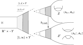
Figure 8. Defining the spinor bundle $S_{(A,\varPhi)}^{\prime}$ over $M_{\tau}^{\prime}$.

Notice that if $u\in\mathcal{G}(M_{\tau})$ then $h_{u\cdot(A,\varPhi)}=u^{-1}h_{(A,\varPhi)}$ and so we can easily build an isomorphism

$$u^{\#}:S_{(A,\varPhi)}^{\prime}\rightarrow S_{u\cdot(A,\varPhi)}^{\prime}$$

Our next job is to construct a configuration on the spinor bundle $S_{(A,\varPhi)}^{\prime}$ over $M_{\tau}^{\prime}$. For this we recall a family of cut-off functions described in section 2.2.1 of [32] . Let $\chi(t)$ be a smooth decreasing function such that

$$\chi(t)=\begin{cases}0&t\geq 1\\ 1&t\leq 0\end{cases}$$

and define

$$\chi_{\tau}(t)=\chi\left(\frac{t-\tau}{N_{0}}+1\right)=\begin{cases}0&t\geq\tau\\ 1&t\leq\tau-N_{0}\end{cases}$$

where $N_{0}$ is a number that is fixed later to control the derivatives of $\chi_{\tau}$. With the help of this function define $S_{(A,\varPhi)}^{\prime}$ as follows:

$\bullet$ On the region $M_{\tau}^{\prime}\cap\{\sigma_{\tau}^{\prime}<\tau\}$ we can identify the structures on $M_{\tau}$ with $M_{\tau}^{\prime}$ and so $(A,\varPhi)\mid_{M_{\tau}\cap\{\sigma_{\tau}<\tau\}}$ defines a configuration on $S_{(A,\varPhi)}^{\prime}\mid_{M_{\tau}^{\prime}\cap\{\sigma_{\tau}^{\prime}\leq\tau\}}$.

$\bullet$ On the region $M_{\tau}^{\prime}\cap\{\sigma_{\tau}^{\prime}\geq T\}$ we can write $\varPhi$ as a pair $(\alpha,\beta)$ and $A$ as $A=A_{0,\tau}+a$ so if we regard $h_{(A,\varPhi)}$ as a gauge transformation (the one that is used to transition on the annulus $M_{\tau}^{\prime}\cap\{T\leq\sigma_{\tau}^{\prime}\leq\tau\}$) then

$$h_{(A,\varPhi)}\cdot(A,\varPhi)$$

$$= h_{(A,\varPhi)}\cdot(A_{0,\tau}+a,(\alpha,\beta))$$

$$= \left(A_{0,\tau}+a-\frac{\alpha}{|\alpha|}d\left(\frac{|\alpha|}{\alpha}\right),\left(|\alpha|,\frac{|\alpha|}{\alpha}\beta\right)\right)$$

$$\equiv \left(A_{0,\tau}+\hat{a},(\hat{\alpha},\hat{\beta})\right)$$

Notice that $\hat{\alpha}$ is a real function with $\hat{\alpha}\geq\frac{1}{2}$. Therefore we define on $M_{\tau}^{\prime}\cap\{\sigma_{\tau}^{\prime}\geq T\}$

$$(A,\varPhi)^{\#}\equiv(A_{0,\tau}^{\prime}+(\chi_{\tau}\circ\sigma_{\tau}^{\prime})\hat{a},(\hat{\alpha}^{\chi_{\tau}\circ\sigma_{\tau}^{\prime}},(\chi_{\tau}\circ\sigma_{\tau}^{\prime})\hat{\beta}))$$

$\bullet$ On the end $\{\sigma_{\tau}^{\prime}\geq\tau\}$ we set

$$(A,\varPhi)^{\#}=(A_{0,\tau}^{\prime},\varPhi_{0,\tau}^{\prime})$$

Since the construction is compatible with the gauge group action in the sense that

$$u^{\#}\cdot(A,\varPhi)^{\#}=(u\cdot(A,\varPhi))^{\#}$$

we have constructed our pre-gluing map

(60) $$\#:\mathcal{M}(M_{\tau},\mathfrak{s}_{\tau},[\mathfrak{c}])\rightarrow(\mathcal{C}/\mathcal{G})(M_{\tau}^{\prime})$$

Lemma (51) of the Appendix guarantees the following exponential decay estimate: there is a $\delta>0$ and $T$ large enough such that for every $N_{0}\geq 1,k\in\mathbb{N}$ , $\tau$ satisfying $\tau\geq T+N_{0}$ and every solution $(A,\varPhi)$ of the Seiberg-Witten equations on $M_{\tau}$, we have that $(A,\varPhi)^{\#}$ satisfies the Seiberg-Witten equations on $\{\sigma_{\tau}^{\prime}\leq T\}\subset M_{\tau}^{\prime}$ and

(61) $$|\mathfrak{F}_{\mathfrak{p}_{M_{\tau}^{\prime}}}(A,\varPhi)^{\#}|_{C^{k}(g_{\tau}^{\prime},A^{\#})}\leq c_{k}e^{-\delta\sigma_{\tau}}$$

on $\{\sigma_{\tau}^{\prime}\geq T\}\subset M_{\tau}^{\prime}$.

Our objective now is to modify the pre-gluing map $\#:M(M_{\tau},\mathfrak{s}_{\tau},[\mathfrak{c}])\rightarrow(\mathcal{C}/\mathcal{G})(M_{\tau}^{\prime})$ to obtain a gluing map (Theorem 3.1.9 [32])

$$\mathfrak{G}_{\tau}:\mathcal{M}(M_{\tau},\mathfrak{s}_{\tau},[\mathfrak{c}])\rightarrow\mathcal{M}(M_{\tau}^{\prime},\mathfrak{s}_{\tau}^{\prime},[\mathfrak{c}])$$

We want to define $\mathfrak{G}_{\tau}$ at the level of configuration spaces in such a way that is gauge equivariant. Our proposal is that this map should decompose as

(62) $$\mathfrak{G}_{\tau}(A,\varPhi)=(A,\varPhi)^{\#}+\left(\mathcal{D}_{(A,\varPhi)^{\#}}\mathfrak{F}_{\mathfrak{p}_{M_{\tau}^{\prime}}}\right)^{*}(b^{\prime},\psi^{\prime})$$

where $(b^{\prime},\psi^{\prime})\in L_{k,A}^{2}(i\mathfrak{su}(S_{\tau}^{\prime+})\oplus S_{\tau}^{\prime-})$ is the quantity that needs to be determined.

Here $\mathcal{D}_{(A,\varPhi)^{\#}}\mathfrak{F}_{\mathfrak{p}_{M_{\tau}^{\prime}}}$ denotes the linearization of the perturbed Seiberg-Witten map $\mathfrak{F}_{\mathfrak{p}_{M_{\tau}^{\prime}}}$. In the old days of Seiberg-Witten theory, where only the curvature equation was perturbed by some imaginary-valued self-dual two-form, this linearized map $\mathcal{D}_{(A,\varPhi)^{\#}}\mathfrak{F}_{\mathfrak{p}_{M_{\tau}^{\prime}}}$ would coincide with the linearization of the unperturbed Seiberg-Witten map $\mathcal{D}_{(A,\varPhi)^{\#}}\mathfrak{F}$, since the perturbations where independent of the configuration $(A,\varPhi)^{\#}$ being used. In fact, analyzing the formula (57), we can see that the discrepancy between these two maps is due to the (abstract) perturbations used on the cylindrical end, so to emphasize this point we may sometimes write $\mathcal{D}_{\mathfrak{q},(A,\varPhi)^{\#}}\mathfrak{F}$ instead of the more precise notation $\mathcal{D}_{(A,\varPhi)^{\#}}\mathfrak{F}_{\mathfrak{p}_{M_{\tau}^{\prime}}}$.

Recall that the perturbed Seiberg-Witten equation is

$$\mathfrak{F}_{\mathfrak{p}_{M_{\tau}^{\prime}}}(A,\varPhi)=\mathfrak{F}(A,\varPhi)+\mathfrak{p}_{M_{\tau}^{\prime}}(A,\varPhi)=0$$

By definition, we want $\mathfrak{G}_{\mathfrak{\tau}}(A,\varPhi)$ to solve the previous equation which means that

$$\mathfrak{F}\mathfrak{G}_{\tau}(A,\varPhi)+\mathfrak{p}_{M_{\tau}^{\prime}}\mathfrak{G}_{\mathfrak{\tau}}(A,\varPhi)=0$$

and implicitly we want to think of the previous equation as depending on $(b^{\prime},\psi^{\prime})$ when we write $\mathfrak{G}_{\tau}(A,\varPhi)$ in an explicit way as in (62) . In order to write this equation in terms of $(b^{\prime},\psi^{\prime})$, one needs to perform many tedious calculations which will be included in the author’s thesis but not here in order to simplify the exposition. These can be found on pages $88$ through $96$ of [10].

To explain the end result, it is good to compare our calculation with equation 3.2 in [32]. Following the notation in section 3 of [32], we define first the “perturbed Seiberg-Witten Laplacian”

(63) $$\triangle_{2,\mathfrak{q},(A,\varPhi)^{\#}}=\left(\mathcal{D}_{(A,\varPhi)^{\#}}\mathfrak{F}_{\mathfrak{q}}\right)\circ\left(\mathcal{D}_{(A,\varPhi)^{\#}}\mathfrak{F}_{\mathfrak{q}}\right)^{*}$$

and the quadratic map

$$\mathcal{Q}(a,\phi)=(-(\phi\phi^{*})_{0},\rho(a)\phi)$$

Finally, define the perturbation term

$$P(b^{\prime},\psi^{\prime})=\mathfrak{p}_{M_{\tau}^{\prime}}(\mathfrak{G}(A,\varPhi))-\mathfrak{p}_{M_{\tau}^{\prime}}(A,\varPhi)^{\#}-\left(\mathcal{D}_{(A,\varPhi)}\hat{\mathfrak{q}}\right)\circ\left(\mathcal{D}_{(A,\varPhi)^{\#}}\mathfrak{F}_{\mathfrak{q}}\right)^{*}$$

One can then show the following:

Theorem 37.

The configuration $\mathfrak{G}_{\mathfrak{q}}(A,\varPhi)=(A,\varPhi)^{\#}+\left(\mathcal{D}_{\mathfrak{q},(A,\varPhi)^{\#}}\mathfrak{F}_{\mathfrak{q}}\right)^{*}(b^{\prime},\psi^{\prime})$ is a solution to the perturbed Seiberg Witten equations $\mathfrak{F}_{\mathfrak{p}_{M_{\tau}^{\prime}}}\mathfrak{G}_{\mathfrak{q}}(A,\varPhi)=0$ if and only if

(64) $$\triangle_{2,\mathfrak{q},(A,\varPhi)^{\#}}(b^{\prime},\psi^{\prime})+\mathcal{Q}\circ\left(\mathcal{D}_{(A,\varPhi)^{\#}}\mathfrak{F}_{\mathfrak{q}}\right)^{*}(b^{\prime},\psi^{\prime})+P(b^{\prime},\psi^{\prime})=-\mathfrak{F}_{\mathfrak{p}_{M_{\tau}^{\prime}}}(A,\varPhi)^{\#}$$

Notice that the term $P(b^{\prime},\psi^{\prime})$ is a new term that does not appear in the usual linearization of the Seiberg Witten equations. This appears solely due to the presence of the abstract perturbations used in [26]. To solve this equation we will need a sharp version of the contraction mapping theorem.

Namely, the basic idea is to define

$$V_{\mathfrak{q}}=\triangle_{2,\mathfrak{q},(A,\varPhi)^{\#}}(b^{\prime},\psi^{\prime})$$

Our intention is to show that $\triangle_{2,\mathfrak{q},(A,\varPhi)^{\#}}$ is invertible so that if we define $S_{\mathfrak{q},(A,\varPhi)^{\#}}(V_{\mathfrak{q}})$ as

$$S_{\mathfrak{q},(A,\varPhi)^{\#}}(V_{\mathfrak{q}})\equiv-\mathcal{Q}\circ\left[\left(\mathcal{D}_{(A,\varPhi)^{\#}}\mathfrak{F}_{\mathfrak{q}}\right)^{*}\right]\left(\triangle_{2,\mathfrak{q},(A,\varPhi)^{\#}}^{-1}V_{\mathfrak{q}}\right)-P\left(\triangle_{2,\mathfrak{q},(A,\varPhi)^{\#}}^{-1}V_{\mathfrak{q}}\right)$$

the gluing equation (64) that we need to solve can be written as

$$V_{\mathfrak{q}}=S_{\mathfrak{q},(A,\varPhi)^{\#}}(V_{\mathfrak{q}})-\mathfrak{F}_{\mathfrak{p}_{M_{\tau}^{\prime}}}(A,\varPhi)^{\#}$$

The solution of this equation will be guaranteed once we shows the hypothesis of Proposition 2.3.5 in [32] are satisfied. Therefore, we will show first that $\triangle_{2,\mathfrak{q},(A,\varPhi)^{\#}}$ is indeed invertible.

6.4 Invertibility of $\triangle_{2,\mathfrak{q},(A,\varPhi)^{\#}}$

In this section we seek a version of Proposition 3.1.2 and Corollary 3.1.6 in [32] , namely, we want to show that:

Theorem 38.

For each $k\geq 0$ there exists a constant $c_{k}>0$ such that for every $\tau$ large enough, every $N_{0}\geq 1$ and every solution $(A,\varPhi)$ of the Seiberg-Witten equations on $M_{\tau}$ belonging to the zero dimensional strata of $\mathcal{M}(M_{\tau},\mathfrak{s}_{\tau},[\mathfrak{c}])$, the operator

$$\triangle_{2,\mathfrak{q},(A,\varPhi)^{\#}}:L_{k+2,A^{\#}}^{2}(M_{\tau}^{\prime},g_{\tau}^{\prime})\rightarrow L_{k,A^{\#}}^{2}(M_{\tau}^{\prime},g_{\tau}^{\prime})$$

$$(b^{\prime},\psi^{\prime})\rightarrow\left(\mathcal{D}_{\mathfrak{q},(A,\varPhi)^{\#}}\mathfrak{F}\right)\circ(\mathcal{D}_{\mathfrak{q},(A,\varPhi)^{\#}}\mathfrak{F})^{*}(b^{\prime},\psi^{\prime})$$

is an isomorphism, and moreover, its inverse $\triangle_{2,\mathfrak{q},(A,\varPhi)^{\#}}^{-1}$ satisfies for all $(b^{\prime},\psi^{\prime})$

$$c_{k}\|(b^{\prime},\psi^{\prime})\|_{L_{k+1}^{2}(g_{\tau}^{\prime},A^{\#})}\geq\|\triangle_{2,\mathfrak{q},(A,\varPhi)^{\#}}^{-1}(b^{\prime},\psi^{\prime})\|_{L_{k+3}^{2}(g_{\tau}^{\prime},A^{\#})}$$

Before proceeding we make a few clarifications:

Remark 39.

a) The norms used for the gluing arguments are gauge equivariant norms, which depend on the configuration $(A,\varPhi)^{\#}$ being used, as can be seen from our use of subscript in the formulas for the Sobolev spaces.

b) Our hypothesis regarding the fact that the solution $[(A,\varPhi)]$ belongs to the $0$ dimensional strata of the moduli space $\mathcal{M}(M_{\tau},\mathfrak{s}_{\tau},[\mathfrak{c}])$ has to do with the fact that we will need to find uniform bounds which we will depend (partly) on the norms of these solutions. Since we are using gauge equivariant norms and the zero dimensional moduli spaces $\mathcal{M}_{0}(M_{\tau},\mathfrak{s}_{\tau},[\mathfrak{c}])$ are compact, for a fixed $\tau$ there can only be finitely many terms to worry about. Clearly, a priori the bounds that we get still depend on the value of $\tau$ chosen, but we will see that a transversality argument will help us control these quantities in a way that is $\tau$-independent. It should be pointed out that this assumption regarding the zero dimensional strata is not that different from the hypothesis used in other gluing arguments. See for example Theorem 4.17 in [9] (which uses a compactness assumption as well) or Theorem 18.3.5 in [26] (which describes all small solutions of a moduli space).

c) The strategy that we will use to prove the invertibility of $\triangle_{2,\mathfrak{q},(A,\varPhi)^{\#}}$ differs from the one employed by [32] mainly because of the following reasons. The way [32] controlled the norm $\triangle_{2,\mathfrak{q},(A,\varPhi)^{\#}}$ was by first controlling the norm a different operator $\square_{(A,\varPhi)^{\#}}=Q_{\mathfrak{q},(A,\varPhi)}\circ Q_{\mathfrak{q},(A,\varPhi)}^{*}$ (defined in the proof of Proposition 3.1.2) and then relating the norms of these two operators through equation (3.6) in their paper. However, these norms were only comparable because their equation (3.7), which uses the fact that $D_{A^{\#}}\varPhi^{\#}$ is almost zero. This was true in their case because the usual Seiberg-Witten equations do not perturb the Dirac equation and since $(A,\varPhi)^{\#}$ is very close to being a solution this means that $\varPhi^{\#}$ is very close to being a harmonic spinor with respect to $D_{A^{\#}}$. However, the abstract perturbations $\mathfrak{q}$ used in [26] do modify the Dirac equation, so any clear relationship between $\square_{(A,\varPhi)^{\#}}$ and $D_{A^{\#}}$ is lost.

The proof of this theorem will follow a splicing argument similar to the one used in section 4.2.2 of [30] (or section 4.4 in [9]). Namely, we will separate the manifold $M_{\tau}^{\prime}$ into two pieces (see Figure (8)) and show the following:

Lemma 40.

We can find two operators

$$\triangle_{2,\mathfrak{q},(A,\varPhi),cyl}^{-1}:L^{2}(M_{\tau})\rightarrow L_{2,A}^{2}(M_{\tau})$$

and

(65) $$\triangle_{2,\widetilde{(A,\varPhi)},end}^{-1}:L^{2}(N_{\tau}^{+})\rightarrow L_{2,\tilde{A}}^{2}(N_{\tau}^{+})$$

with the following properties:

a) $\triangle_{2,\mathfrak{q},(A,\varPhi),cyl}^{-1}$ is the inverse to the Seiberg-Witten “Laplacian” defined as in equation (63)

$$\triangle_{2,\mathfrak{q},(A,\varPhi)}=\left(\mathcal{D}_{(A,\varPhi)}\mathfrak{F}_{\mathfrak{q}}\right)\circ\left(\mathcal{D}_{(A,\varPhi)}\mathfrak{F}_{\mathfrak{q}}\right)^{*}:L_{2,A}^{2}(M_{\tau})\rightarrow L^{2}(M_{\tau})$$

b) Likewise, there is a Seiberg-Witten Laplacian

$$\triangle_{2,(A,\varPhi)^{\#},end}=\left(\mathcal{D}_{(A,\varPhi)^{\#}}\mathfrak{F}\right)\circ\left(\mathcal{D}_{(A,\varPhi)^{\#}}\mathfrak{F}\right)^{*}:L_{2,A}^{2}(M_{\tau}^{\prime}\backslash(\mathbb{R}^{+}\times-Y))\rightarrow L^{2}(M_{\tau}^{\prime}\backslash(\mathbb{R}^{+}\times-Y))$$

which can be extended to an invertible Seiberg-Witten Laplacian

$$\triangle_{2,\widetilde{(A,\varPhi)},end}=\left(\mathcal{D}_{\widetilde{(A,\varPhi)}}\mathfrak{F}_{\eta}\right)\circ\left(\mathcal{D}_{\widetilde{(A,\varPhi)}}\mathfrak{F}_{\eta}\right)^{*}:L_{2,\tilde{A}}^{2}(N_{\tau}^{+})\rightarrow L^{2}(N_{\tau}^{+})$$

where $N_{\tau}^{+}$ is a capped-off version of $M_{\tau}^{\prime}\backslash(\mathbb{R}^{+}\times-Y)$ defined in the proof of this lemma.

Remark 41.

As we will explain in the proof, $\widetilde{(A,\varPhi)}$ denotes an extension of $(A,\varPhi)^{\#}$ to the manifold $N_{\tau}^{+}$, which agrees with $(A,\varPhi)^{\#}$ on the region $Z_{\tau}\backslash\left([1,T/2)\times Y\right)$. Because of this we will write in the following lemmas $\triangle_{2,\widetilde{(A,\varPhi)},end}^{-1}$ as $\triangle_{2,(A,\varPhi)^{\#},end}^{-1}$.

Also, our construction of $\triangle_{2,\widetilde{(A,\varPhi)},end}$ is not very sharp since we are using this operator as a proxy for a parametrix argument that will be important in the next section.

Proof.

We will divide $M_{\tau}^{\prime}$ into two regions, each of which is the natural location where each of the operators from the statement of the lemma can be considered.

$\bullet$ The unperturbed region $(\mathbb{R}^{+}\times-Y)\cup[1,T]\times Y$ [construction of $\triangle_{2,\mathfrak{q},(A,\varPhi),cyl}^{-1}$]:

This refers to the region where $(A,\varPhi)^{\#}=(A,\varPhi)$, that is, the solution $(A,\varPhi)$ was not modified. Notice that this includes the cylinder $\mathbb{R}^{+}\times-Y$ and the section of the cone $[1,T]\times Y$ and we can use the fact that the moduli space on $(M_{\tau},g_{\tau})$ is regular to conclude that $Q_{\mathfrak{q},(A,\varPhi)}$ is surjective on $M_{\tau}$ [26, Def. 14.5.6]. Using that $Q_{\mathfrak{q},(A,\varPhi)}=\mathcal{D}_{(A,\varPhi)}\mathfrak{F}_{\mathfrak{q}}\oplus\mathbf{d}_{(A,\varPhi)}^{*}$ we conclude that $\mathcal{D}_{(A,\varPhi)}\mathfrak{F}_{\mathfrak{q}}$ must be surjective as well.

Now, since $Q_{\mathfrak{q},(A,\varPhi)}$ is a Fredholm operator we can easily see that $Q_{\mathfrak{q},(A,\varPhi)}^{*}$ must be injective. Moreover $Q_{\mathfrak{q},(A,\varPhi)}^{*}=\left(\mathcal{D}_{(A,\varPhi)}\mathfrak{F}_{\mathfrak{q}}\right)^{*}\oplus\mathbf{d}_{(A,\varPhi)}$ so $\left(\mathcal{D}_{(A,\varPhi)}\mathfrak{F}_{\mathfrak{q}}\right)^{*}$ must be injective as well.

In particular, it is not difficult to check that because of this $\triangle_{2,\mathfrak{q},(A,\varPhi)}$ will be invertible as an operator on $M_{\tau}$. To emphasize that we care about this operator when applied to sections supported on the unperturbed region (which contains the cylinder) we will write the inverse as a map

$$\triangle_{2,\mathfrak{q},(A,\varPhi),cyl}^{-1}:L^{2}(M_{\tau})\rightarrow L_{2,A}^{2}(M_{\tau})$$

$\bullet$ The perturbed region $M_{\tau}^{\prime}\backslash(\mathbb{R}^{+}\times-Y)$ [construction of $\triangle_{2,\widetilde{(A,\varPhi)},end}^{-1}$]:

This refers to the region where $(A,\varPhi)^{\#}$ and $(A,\varPhi)$ do not necessarily agree. Notice that this includes the region $[1,\tau]\times Y$ together with remaining piece of the $AFAK$ end $Z^{\prime}$. Moreover $\triangle_{2,\mathfrak{q},(A,\varPhi)^{\#}}=\triangle_{2,(A,\varPhi)^{\#}}$ on this part of the manifold.

We now follow section 3.3 in [32], which uses a similar idea to what we are about to do, albeit for dealing with the orientability of the moduli spaces.

Recall that we can find an almost complex manifold $N$ with boundary $\partial N=Y$ [19, Lemma 4.4]. We can glue this piece to $M_{\tau}^{\prime}\backslash(\mathbb{R}^{+}\times-Y)$ along the cone $[1,\tau]\times Y$ to obtain a manifold $N_{\tau}^{+}$ without boundary and with an AFAK end (so these are precisely the class of manifolds that were studied in [19].

In particular, since an almost complex structure now exists globally on $N_{\tau}^{+}$ we can talk about the canonical pair $(A_{0,\tau}^{\prime},\varPhi_{0,\tau}^{\prime})$ globally, which we will denote as $\widetilde{(A_{0,\tau}^{\prime},\varPhi^{\prime}_{0,\tau}})$. This configuration is almost a solution to the Seiberg-Witten equations

$$\begin{cases}\frac{1}{2}\rho(F_{A^{t}}^{+})-(\varPhi\varPhi^{*})_{0}=\frac{1}{2}\rho(F_{\tilde{A}_{0,\tau}^{\prime}}^{+})-(\tilde{\varPhi}_{0,\tau}^{\prime}\tilde{\varPhi}_{0,\tau}^{\prime*})_{0}\\ D_{A}\varPhi=0\end{cases}$$

on $N_{\tau}^{+}$. The only reason why we say almost is that on the almost complex manifold $N$ we attached, the nondegenerate two form $\omega_{N}$ induced by the metric and almost complex structure on $N$ may not give rise to a symplectic form. In general, there is torsion (a Lee-Gauduchon) form $\eta_{N}$ characterized by

$$d\omega_{N}=\omega_{N}\wedge\eta$$

In particular, $\widetilde{(A_{0,\tau}^{\prime},\varPhi^{\prime}_{0,\tau}})$ will be a solution to the equations

$$\begin{cases}\frac{1}{2}\rho(F_{A^{t}}^{+})-(\varPhi\varPhi^{*})_{0}=\frac{1}{2}\rho(F_{\tilde{A}_{0,\tau}^{\prime}}^{+})-(\tilde{\varPhi}_{0,\tau}^{\prime}\tilde{\varPhi}_{0,\tau}^{\prime*})_{0}\\ D_{A}\varPhi=\frac{1}{4}\rho(\eta)\varPhi\end{cases}$$

on $N_{\tau}^{+}$. Associated to these Seiberg-Witten equations, there is a corresponding operator $Q_{\eta,(\tilde{A}_{0,\tau}^{\prime},\tilde{\varPhi}_{0,\tau}^{\prime})}$. The discussion in [32, Section 3.3.1] in fact shows that the moduli space of solutions is unobstructed at $\widetilde{(A_{0,\tau}^{\prime},\varPhi^{\prime}_{0,\tau}})$, that is, both of the operators $Q_{\eta,(\tilde{A}_{0,\tau}^{\prime},\tilde{\varPhi}_{0,\tau}^{\prime})}$ and $Q_{\eta,(\tilde{A}_{0,\tau}^{\prime},\tilde{\varPhi}_{0,\tau}^{\prime})}^{*}$ are invertible. Hence, as in the argument from the first part of this lemma we can conclude that the corresponding operator

$$\triangle_{2,\widetilde{(A_{0,\tau}^{\prime},\varPhi^{\prime}_{0,\tau}}),end}=\left(\mathcal{D}_{\widetilde{(A_{0,\tau}^{\prime},\varPhi^{\prime}_{0,\tau}})}\mathfrak{F}_{\eta}\right)\circ\left(\mathcal{D}_{\widetilde{(A_{0,\tau}^{\prime},\varPhi^{\prime}_{0,\tau}})}\mathfrak{F}_{\eta}\right)^{*}:L_{2,\tilde{A}_{0,\tau}^{\prime}}^{2}(N_{\tau}^{+})\rightarrow L^{2}(N_{\tau}^{+})$$

is invertible.

Now we explain what to do with the other configurations $(A,\varPhi)^{\#}$. We define $\widetilde{(A,\varPhi)}$ as an extension to $N_{\tau}^{+}$ in such a way that:

a) $\widetilde{(A,\varPhi)}$ agrees with $\widetilde{(A_{0,\tau}^{\prime},\varPhi^{\prime}_{0,\tau}})$ on the region $N\cup\left([1,T/4]\times Y\right)$.

b) $\widetilde{(A,\varPhi)}$ agrees with $(A,\varPhi)^{\#}$ on the region $N_{\tau}^{+}\backslash\left(N\cup\left([1,T/2)\times Y\right)\right)=Z_{\tau}\backslash\left([1,T/2)\times Y\right)$.

c) $\widetilde{(A,\varPhi)}$ interpolates between $\widetilde{(A_{0,\tau}^{\prime},\varPhi^{\prime}_{0,\tau}})$ and $(A,\varPhi)^{\#}$ on the remaining region $[T/4,T/2]\times Y$.

In particular, since $(A,\varPhi)^{\#}$ also agrees $\widetilde{(A_{0,\tau}^{\prime},\varPhi^{\prime}_{0,\tau}})$ whenever $t>\tau$, we find that with $\widetilde{(A,\varPhi)}$ differs from $\widetilde{(A_{0,\tau}^{\prime},\varPhi^{\prime}_{0,\tau}})$ at most on the region $[T/4,\tau]\times Y$ . Since being an invertible operator is an open condition, if we wanted to show that the corresponding operator $\triangle_{2,(\tilde{A},\tilde{\varPhi}),end}$ is invertible, it would suffice to show that it is close in the operator norm to $\triangle_{2,\widetilde{(A_{0,\tau}^{\prime},\varPhi^{\prime}_{0,\tau}}),end}$.

In fact, one can compare in a very explicit fashion both operators (we do something very similar in the next lemma for example hence we omit some of the details for now), so we just need to have chosen $T$ from the beginning of our gluing construction in section $6.3$ in such a way that this norm condition is satisfied, so that $\triangle_{2,(\tilde{A},\tilde{\varPhi}),end}$ ends up being invertible (again, a similar argument appears in the next lemma). ∎

Lemma 42.

For any solution $(A,\varPhi)$ to the Seiberg Witten equations on the manifold $M_{\tau}$, the operator $\triangle_{2,\mathfrak{q},(A,\varPhi)^{\#}}$ is a Fredholm operator on $M_{\tau}^{\prime}$.

Proof.

We will introduce some cutoff functions that will allow us to follow the usual splicing arguments: these will be denoted $\eta_{cyl}$ and $\eta_{end}$. They satisfy the following properties:

$\bullet$ $0\leq\eta_{cyl},\eta_{end}\leq 1$ and $\eta_{cyl}^{2}+\eta_{end}^{2}=1$.

$\bullet$ $\eta_{cyl}$ is supported on the unperturbed region. Moreover, $\eta_{cyl}\equiv 1$ on a small neighborhood of the region $\mathbb{R}^{+}\times-Y\cup[1,T/2]\times Y$ . In particular, the gradient of $\eta_{cyl}$ is supported on the fixed region $[1,T]\times Y$.

$\bullet$ $\eta_{end}$ is supported on the perturbed region. Moreover, $\eta_{end}\equiv 1$ on a small neighborhood of $([T,\tau]\times Y)\cup\{Z^{\prime}\cap\{\sigma_{Z^{\prime}}>1/\tau\}$. In particular, the gradient of $\eta_{end}$ is supported on the fixed region $[1,T]\times Y$. Notice that also $\eta_{end}$ will vanish in a small neighborhood of $\{T/2\}\times Y$, since $\eta_{cyl}$ is equal to $1$ near that slice.

$\bullet$ For $\eta=\eta_{cyl},\eta_{end}$ we have $|\nabla^{n}\eta|\leq\left(\frac{2}{T}\right)^{n}$ .

Our proto-inverse will be the operator

$$\tilde{\triangle}_{2,\mathfrak{q},(A,\varPhi)^{\#}}^{-1}:L^{2}(M_{\tau}^{\prime},g_{\tau}^{\prime})\rightarrow L_{2}^{2}(M_{\tau}^{\prime},g_{\tau}^{\prime})$$

$$(b^{\prime},\psi^{\prime})\rightarrow\eta_{cyl}\triangle_{2,\mathfrak{q},(A,\varPhi),cyl}^{-1}[\eta_{cyl}(b^{\prime},\psi^{\prime})]+\eta_{end}\triangle_{2,(A,\varPhi)^{\#},end}^{-1}[\eta_{end}(b^{\prime},\psi^{\prime})]$$

We will see that $\tilde{\triangle}_{2,\mathfrak{q},(A,\varPhi)^{\#}}^{-1}$ provides a parametrix for $\triangle_{2,\mathfrak{q},(A,\varPhi)^{\#}}$: this is because

$$\triangle_{2,\mathfrak{q},(A,\varPhi)^{\#}}\left[\tilde{\triangle}_{2,\mathfrak{q},(A,\varPhi)^{\#}}^{-1}(b^{\prime},\psi^{\prime})\right]$$

$$= \triangle_{2,\mathfrak{q},(A,\varPhi)^{\#}}\left[\eta_{cyl}\triangle_{2,\mathfrak{q},(A,\varPhi),cyl}^{-1}[\eta_{cyl}(b^{\prime},\psi^{\prime})]+\eta_{end}\triangle_{2,(A,\varPhi)^{\#},end}^{-1}[\eta_{end}(b^{\prime},\psi^{\prime})]\right]$$

$$= \left\{\mathcal{D}_{(A,\varPhi)}\eta_{cyl},\triangle_{2,\mathfrak{q},(A,\varPhi),cyl}^{-1}[\eta_{cyl}(b^{\prime},\psi^{\prime})]\right\}+\eta_{cyl}^{2}(b^{\prime},\psi^{\prime})$$

$$+\left\{\mathcal{D}_{(A,\varPhi)}\eta_{end},\triangle_{2,(A,\varPhi)^{\#},end}^{-1}[\eta_{end}(b^{\prime},\psi^{\prime})]\right\}+\eta_{end}^{2}(b^{\prime},\psi^{\prime})$$

$$+\left\{\mathcal{D}_{(A,\varPhi)}\eta_{cyl},\mathcal{D}_{(A,\varPhi)}\left(\triangle_{2,\mathfrak{q},(A,\varPhi),cyl}^{-1}[\eta_{cyl}(b^{\prime},\psi^{\prime})]\right)\right\}+\left\{\mathcal{D}_{(A,\varPhi)}\eta_{end},\mathcal{D}_{(A,\varPhi)}\left(\triangle_{2,(A,\varPhi)^{\#},end}^{-1}[\eta_{end}(b^{\prime},\psi^{\prime})]\right)\right\}$$

$$= \left\{\mathcal{D}_{(A,\varPhi)}\eta_{cyl},\triangle_{2,\mathfrak{q},(A,\varPhi),cyl}^{-1}[\eta_{cyl}(b^{\prime},\psi^{\prime})]\right\}+\left\{\mathcal{D}_{(A,\varPhi)}\eta_{end},\triangle_{2,(A,\varPhi)^{\#},end}^{-1}[\eta_{end}(b^{\prime},\psi^{\prime})]\right\}+(b^{\prime},\psi^{\prime})$$

$$+\left\{\mathcal{D}_{(A,\varPhi)}\eta_{cyl},\mathcal{D}_{(A,\varPhi)}\left(\triangle_{2,\mathfrak{q},(A,\varPhi),cyl}^{-1}[\eta_{cyl}(b^{\prime},\psi^{\prime})]\right)\right\}+\left\{\mathcal{D}_{(A,\varPhi)}\eta_{end},\mathcal{D}_{(A,\varPhi)}\left(\triangle_{2,(A,\varPhi)^{\#},end}^{-1}[\eta_{end}(b^{\prime},\psi^{\prime})]\right)\right\}$$

Here the notation $\{\cdot,\cdot\}$ is used to indicate a bilinear pointwise multiplication between some (higher order) derivatives of the cutoff functions and the elements in the domain. Also, the notation $\mathcal{D}_{(A,\varPhi)}\eta_{cyl}$ means that this expression involves (higher order) derivatives of the perturbation (and a priori the configuration $(A,\varPhi)$, but whose precise form is not important to us.

Notice that the first and last two terms are supported on the compact subset $[1,T]\times Y$, where $(A,\varPhi)^{\#}=(A,\varPhi)$. Also, we dropped the dependence on $\mathfrak{q}$ for the derivatives $\mathcal{D}_{(A,\varPhi)}\eta_{\bullet}$ since this perturbation affects only the cylindrical region. To analyze if there is any dependence of $\mathcal{D}_{(A,\varPhi)}\eta_{\bullet}$ on $(A,\varPhi)$, we will study $\mathcal{D}_{(A,\varPhi)}\eta_{cyl}$ since the other case is exactly the same. We need to compute

(66) $$\triangle_{2,\mathfrak{q},(A,\varPhi)^{\#}}\left(\eta_{cyl}(b_{cyl},\psi_{cyl})\right)$$

where we defined

$$(b_{cyl},\psi_{cyl})\equiv\triangle_{2,\mathfrak{q},(A,\varPhi),cyl}^{-1}[\eta_{cyl}(b^{\prime},\psi^{\prime})]$$

Notice that we may write

$$\triangle_{2,\mathfrak{q},(A,\varPhi)^{\#}}=\left(\mathcal{D}_{(A,\varPhi)^{\#}}\mathfrak{F}_{\mathfrak{q}}\right)\circ\left(\mathcal{D}_{(A,\varPhi)^{\#}}\mathfrak{F}_{\mathfrak{q}}\right)^{*}=\left(\mathcal{D}_{(A,\varPhi)^{\#}}\mathfrak{F}_{\mathfrak{}}\right)\circ\left(\mathcal{D}_{(A,\varPhi)^{\#}}\mathfrak{F}_{\mathfrak{}}\right)^{*}=\triangle_{2,(A,\varPhi)^{\#}}$$

since we are only interested in computing (66) on the region $[1,T]\times Y$, where $\eta_{cyl}$ is not constant. The advantage of using this unperturbed Seiberg-Witten ’Laplacian’ is that we can give an explicit formula for it based on the equations (28) and (29). We find that for arbitrary $(b^{\prime},\psi^{\prime})$

$$\triangle_{2,(A,\varPhi)^{\#}}(b^{\prime},\psi^{\prime})= \left(\mathcal{D}_{(A,\varPhi)^{\#}}\mathfrak{F}\right)\left((d^{+})^{*}\rho^{*}b^{\prime}+\rho^{*}(\psi^{\prime}(\varPhi^{\#})^{*}),D_{A^{\#}}^{*}\psi^{\prime}-b^{\prime}\varPhi^{\#}\right)$$

$$= [\rho(d^{+}\left[(d^{+})^{*}\rho^{*}b^{\prime}+\rho^{*}(\psi^{\prime}(\varPhi^{\#})^{*})\right]-\left\{\varPhi^{\#}\left(D_{A^{\#}}^{*}\psi^{\prime}-b^{\prime}\varPhi^{\#}\right)^{*}+\left(D_{A^{\#}}^{*}\psi^{\prime}-b^{\prime}\varPhi^{\#}\right)(\varPhi^{\#})^{*}\right\}_{0},$$

$$D_{A^{\#}}\left(D_{A^{\#}}^{*}\psi^{\prime}-b^{\prime}\varPhi^{\#}\right)+\rho\left((d^{+})^{*}\rho^{*}b^{\prime}+\rho^{*}(\psi^{\prime}(\varPhi^{\#})^{*})\right)\varPhi^{\#}]$$

therefore $\triangle_{2,(A,\varPhi)^{\#}}\left[(\eta_{cyl}b_{cyl},\eta_{cyl}\psi_{cyl})\right]$ becomes

$$[\rho(d^{+}\left[(d^{+})^{*}\rho^{*}\left(\eta_{cyl}b_{cyl}\right)+\rho^{*}(\eta_{cyl}\psi_{cyl}(\varPhi^{\#})^{*})\right]$$

$$- \left\{\varPhi^{\#}\left(D_{A^{\#}}^{*}\left(\eta_{cyl}\psi_{cyl}\right)-(\eta_{cyl}b_{cyl})\varPhi^{\#}\right)^{*}+\left(D_{A^{\#}}^{*}\left(\eta_{cyl}\psi_{cyl}\right)-(\eta_{cyl}b_{cyl})\varPhi^{\#}\right)(\varPhi^{\#})^{*}\right\}_{0}$$

$$+ [\rho(d^{+}\left[(d^{+})^{*}\rho^{*}(\eta_{cyl}b_{cyl})+\rho^{*}(\left(\eta_{cyl}\psi_{cyl}\right)(\varPhi^{\#})^{*})\right]$$

$$- \left\{\varPhi^{\#}\left(D_{A^{\#}}^{*}\left(\eta_{cyl}\psi_{cyl}\right)-(\eta_{cyl}b_{cyl})\varPhi^{\#}\right)^{*}+\left(D_{A^{\#}}^{*}\left(\eta_{cyl}\psi_{cyl}\right)-(\eta_{cyl}b_{cyl})\varPhi^{\#}\right)(\varPhi^{\#})^{*}\right\}$$

Since the Dirac operator $D$ satisfies the Leibniz Rule [1, Prop. 3.38]

$$D(\eta\psi)=\rho(d\eta)\psi+\eta D\psi$$

the only derivatives of $\eta_{cyl}$ that appear are those involving its exterior derivative, which is independent of the configuration $(A,\varPhi)^{\#}$ that is used. A similar story is be true for $\eta_{end}$. Since $\triangle_{2,\mathfrak{q},(A,\varPhi),cyl}^{-1}[\eta_{cyl}(b^{\prime},\psi^{\prime})]$ and $\triangle_{2,(A,\varPhi)^{\#},end}^{-1}[\eta_{end}(b^{\prime},\psi^{\prime})]$ are elements of $L_{2,A^{\#}}^{2}(M_{\tau}^{\prime})$, our previous discussion in fact tells us that the operator

$$K_{(A,\varPhi)}:L^{2}([1,T]\times Y)\rightarrow L^{2}([1,T]\times Y)$$

$$(b^{\prime},\psi^{\prime})\rightarrow \left\{\mathcal{D}\eta_{cyl},\triangle_{2,\mathfrak{q},(A,\varPhi),cyl}^{-1}[\eta_{cyl}(b^{\prime},\psi^{\prime})]\right\}+\left\{\mathcal{D}\eta_{end},\triangle_{2,(A,\varPhi)^{\#},end}^{-1}[\eta_{end}(b^{\prime},\psi^{\prime})]\right\}$$

$$+\left\{\mathcal{D}_{(A,\varPhi)}\eta_{cyl},\mathcal{D}_{(A,\varPhi)}\left(\triangle_{2,\mathfrak{q},(A,\varPhi),cyl}^{-1}[\eta_{cyl}(b^{\prime},\psi^{\prime})]\right)\right\}$$

$$+\left\{\mathcal{D}_{(A,\varPhi)}\eta_{end},\mathcal{D}_{(A,\varPhi)}\left(\triangle_{2,(A,\varPhi)^{\#},end}^{-1}[\eta_{end}(b^{\prime},\psi^{\prime})]\right)\right\}$$

can in fact be regarded as an operator

$$K_{(A,\varPhi)}:L^{2}([1,T]\times Y)\rightarrow L_{2}^{2}([1,T]\times Y)$$

and using the compact inclusion $L_{2}^{2}([1,T]\times Y)\hookrightarrow L^{2}([1,T]\times Y)$ on a compact manifold we conclude that $K_{(A,\varPhi)}$ is a compact operator. This provides the desired parametrix. ∎

The next lemma addresses the bounds on the norms of this parametrix.

Lemma 43.

The norms of the parametrices can be chosen in a uniform way. That is, that there exist a constant $C_{T}$ so that for all solutions $(A,\varPhi)$ we have that $\|K_{(A,\varPhi)}\|\leq\frac{C_{T}}{T}.$ In fact, one can find a constant $C_{\infty}$, independent of $T$ such that $\|K_{(A,\varPhi)}\|\leq\frac{C_{\infty}}{T}$.

Proof.

It is possible to show that the norms of the parametrices are uniform, that is, that there exist a constant $C_{T}$ so that for all solutions $(A,\varPhi)$ we have that $\|K_{(A,\varPhi)}\|\leq\frac{C_{T}}{T}.$ In fact, we will show something better, which is that one could have chosen a constant $C_{\infty}$ which is independent of $T$ , in other words, $\|K_{(A,\varPhi)}\|\leq\frac{C_{\infty}}{T}$.

Notice that a priori the only term that may not seem controllable in terms of $T$ are

(67) $$\left\{\mathcal{D}\eta_{cyl},\triangle_{2,\mathfrak{q},(A,\varPhi),cyl}^{-1}[\eta_{cyl}(b^{\prime},\psi^{\prime})]\right\}\text{ and }\left\{\mathcal{D}_{(A,\varPhi)}\eta_{cyl},\mathcal{D}_{(A,\varPhi)}\left(\triangle_{2,\mathfrak{q},(A,\varPhi),cyl}^{-1}[\eta_{cyl}(b^{\prime},\psi^{\prime})]\right)\right\}$$

We will discuss how to control the first term in (67) since the second is exactly the same. If we take a sequence of solutions $(A_{n},\varPhi_{n})$ on $M_{\tau_{n}}$ then on $[1,T]$ it will converge strongly to a solution $(A_{\infty},\varPhi_{\infty})$ on $Z_{Y,\xi}^{+}$ [this is because of Lemma (53) in the Appendix, based on the compactness theorem 2.2.11 in [32]] and hence for all $(b^{\prime},\psi^{\prime})$

$$\left\{\mathcal{D}\eta_{cyl},\triangle_{2,\mathfrak{q},(A_{n},\varPhi_{n}),cyl}^{-1}[\eta_{cyl}(b^{\prime},\psi^{\prime})]\right\}$$

converges to

$$\left\{\mathcal{D}\eta_{cyl},\triangle_{2,\mathfrak{q},(A_{\infty},\varPhi_{\infty}),cyl}^{-1}[\eta_{cyl}(b^{\prime},\psi^{\prime})]\right\}$$

It is clear then that it would be enough to have a uniform bound on the operator norms

$$\left\|\triangle_{2,\mathfrak{q},(A_{\infty},\varPhi_{\infty})}^{-1}\right\|_{L^{2}(Z_{Y,\xi}^{+})\rightarrow L_{2,A_{\infty}}^{2}(Z_{Y,\xi}^{+})}$$

As we will make more explicitly in the next proof, since we are taking a sequence of solutions $(A_{n},\varPhi_{n})$ which belong to the zero dimensional strata of the moduli spaces $\mathcal{M}(M_{\tau_{n}},\mathfrak{s}_{\tau_{n}},[\mathfrak{c}])$, the limiting solution $(A_{\infty},\varPhi_{\infty})$ must belong to the zero dimensional strata of $\mathcal{M}(Z_{Y,\xi}^{+},\mathfrak{s},[\mathfrak{c}])$, and since we are using gauge equivariant norms, there are only finitely many values the previous operator norm can take (this is related to the second point in the remarks we made after stating the invertibility of the Laplacian). Therefore, we will have the uniform bound for the operator $K_{(A,\varPhi)}$, that is, $\|K_{(A,\varPhi)}\|\leq\frac{C_{\infty}}{T}$ where $C_{\infty}$ is independent of $\tau,T$ and the solutions $(A,\varPhi)$ used.

Therefore, there is no loss of generality in assuming that $T$ was chosen from the beginning so that it would also satisfy the condition

$$\|K_{(A,\varPhi)}\|_{L^{2}([1,T]\times Y)\rightarrow L_{2}^{2}([1,T]\times Y)}\leq\frac{C_{\infty}}{T}\leq\frac{1}{2}$$

for all the solutions of the Seiberg Witten equations on $M_{\tau}$. In particular, from the identity

$$\triangle_{2,\mathfrak{q},(A,\varPhi)^{\#}}\left[\tilde{\triangle}_{2,\mathfrak{q},(A,\varPhi)^{\#}}^{-1}(b^{\prime},\psi^{\prime})\right]=K_{(A,\varPhi)}(b^{\prime},\psi^{\prime})+(b^{\prime},\psi^{\prime})$$

we see that the operator norms satisfy

$$\|\triangle_{2,\mathfrak{q},(A,\varPhi)^{\#}}\tilde{\triangle}_{2,\mathfrak{q},(A,\varPhi)^{\#}}^{-1}-\text{Id}\|_{L_{2,A^{\#}}^{2}(M_{\tau}^{\prime},g_{\tau}^{\prime})\rightarrow L^{2}(M_{\tau}^{\prime},g_{\tau^{\prime}})}\leq\frac{1}{2}$$

In particular we conclude that $\triangle_{2,\mathfrak{q},(A,\varPhi)^{\#}}\tilde{\triangle}_{2,\mathfrak{q},(A,\varPhi)^{\#}}^{-1}$ is invertible and they (and their inverses) are uniformly bounded since

$$\frac{1}{2}\leq\|\triangle_{2,\mathfrak{q},(A,\varPhi)^{\#}}\tilde{\triangle}_{2,\mathfrak{q},(A,\varPhi)^{\#}}^{-1}\|_{L_{2,A^{\#}}^{2}(M_{\tau}^{\prime},g_{\tau}^{\prime})\rightarrow L^{2}(M_{\tau}^{\prime},g_{\tau^{\prime}})}\leq\frac{3}{2}$$

Therefore the inverse of $\triangle_{2,\mathfrak{q},(A,\varPhi)^{\#}}$ is $\tilde{\triangle}_{2,\mathfrak{q},(A,\varPhi)^{\#}}^{-1}\left(\triangle_{2,\mathfrak{q},(A,\varPhi)^{\#}}\tilde{\triangle}_{2,\mathfrak{q},(A,\varPhi)^{\#}}^{-1}\right)^{-1}$. ∎

Returning to our proof of Theorem (38), since $\left(\triangle_{2,\mathfrak{q},(A,\varPhi)^{\#}}\tilde{\triangle}_{2,\mathfrak{q},(A,\varPhi)^{\#}}^{-1}\right)^{-1}$ is uniformly bounded we just need to check that $\tilde{\triangle}_{2,\mathfrak{q},(A,\varPhi)^{\#}}^{-1}$ is uniformly bounded to conclude that $\triangle_{2,\mathfrak{q},(A,\varPhi)^{\#}}$ is uniformly bounded [a similar argument would work to give uniform bounds on $\triangle_{2,\mathfrak{q},(A,\varPhi)^{\#}}^{-1}$] . Looking at the definition of $\tilde{\triangle}_{2,\mathfrak{q},(A,\varPhi)^{\#}}^{-1}$ it becomes clear that it suffices to show that $\eta_{cyl}\triangle_{2,\mathfrak{q},(A,\varPhi),cyl}^{-1}[\eta_{cyl}(b^{\prime},\psi^{\prime})]$ is uniformly bounded.

Here we will use again the assumption we mentioned at the end of the previous proof. Namely, we are now assuming that the gauge equivalence classes of our solutions $(A,\varPhi)\in\mathcal{M}(M_{\tau},\mathfrak{s}_{\tau},[\mathfrak{c}])$ all belong to the zero dimensional strata of the moduli spaces. Since the Laplacians are gauge equivariant in the sense that

$$\triangle_{2,\mathfrak{q},u\cdot(A,\varPhi)}[u\cdot(b,\psi)]=u\cdot\triangle_{2,\mathfrak{q},(A,\varPhi)}(b,\psi)$$

and we are using the gauge equivariant norms $\|\cdot\|_{L_{k,A}^{2}}$ , then for each $\tau$ there are only finitely gauge equivalence classes we need to worry about, which immediately implies that for each $\tau$ we have a control on the Laplacians (and their inverses). Clearly we still need to see what happens as we vary $\tau$.

Let $K$ be a subset of $(\mathbb{R}^{+}\times-Y)\cup([1,\infty)\times Y)$ and use $\|\triangle_{2,\mathfrak{q},(A,\varPhi)}\|_{A,K}$ or $\|\triangle_{2,\mathfrak{q},(A,\varPhi)}^{-1}\|_{A,K}$ to denote the operator norms of $\triangle_{2,\mathfrak{q},(A,\varPhi)}$ and $\triangle_{2,\mathfrak{q},(A,\varPhi)}^{-1}$ when restricted to sections supported on $K$. Clearly if $K\subset K^{\prime}$ then $\|\triangle_{2,\mathfrak{q},(A,\varPhi)}^{-1}\|_{A,K}\leq\|\triangle_{2,\mathfrak{q},(A,\varPhi)}^{-1}\|_{A,K^{\prime}}$ .

Now, recall that we are actually working with a sequence $\tau_{n}$ increasing to $\infty$, so for each $\tau_{n}$ let $[(A_{n},\varPhi_{n})]\in\mathcal{M}_{0}(M_{\tau_{n}},\mathfrak{s}_{\tau},[\mathfrak{c}])$ be a (gauge equivalence class of) solution belonging to the zero dimensional strata. Notice that each compact subset $K\subset(\mathbb{R}^{+}\times-Y)\cup([1,\infty)\times Y)$ eventually belongs to all $M_{\tau_{n}}$ (once $\tau_{n}$ is sufficiently large) so the compactness theorem in this case says that we can choose representatives $(A_{n},\varPhi_{n})$ which converge to a solution $(A_{\infty},\varPhi_{\infty})$ which solves the equations on $Z_{\xi,Y}^{+}$ and this convergence is strong when restricted to the compact subset $K$. In particular, it is clear from this that

(68) $$\|\triangle_{2,\mathfrak{q},(A_{n},\varPhi_{n})}^{-1}\|_{A_{n},K}\rightarrow\|\triangle_{2,\mathfrak{q},(A_{\infty},\varPhi_{\infty})}^{-1}\|_{A_{\infty},K}$$

In fact, we must also have that the limiting solution $(A_{\infty},\varPhi_{\infty})$ belongs to the zero dimensional strata because the different strata are labeled by the index of the operator $Q_{\mathfrak{q},(A,\varPhi)}$ and this index can only decrease (this is how the broken trajectories appear). However, since the index of each element in the sequence was already zero then the index of the limiting configuration would need to be negative if it were to decrease but transversality rules this out, since we do not have negative dimensional moduli spaces. Therefore the convergence is without broken trajectories, that is, $[(A_{\infty},\varPhi_{\infty})]\in\mathcal{M}_{0}(Z_{Y,\xi}^{+},\mathfrak{s},[\mathfrak{c}])$ . In particular, the fact that no energy is lost along the half-cylinder allows us to improve the convergence in (68) to (we will say more about this in a moment)

(69) $$\|\triangle_{2,\mathfrak{q},(A_{n},\varPhi_{n})}^{-1}\|_{A_{n},K_{t}}\rightarrow\|\triangle_{2,\mathfrak{q},(A_{\infty},\varPhi_{\infty})}^{-1}\|_{A_{\infty},K_{t}}$$

where now $K_{t}=(\mathbb{R}^{+}\times-Y)\cup([1,t]\times Y)$ ($t>1$ is arbitrary). In particular,

$$\|\triangle_{2,\mathfrak{q},(A_{\infty},\varPhi_{\infty})}^{-1}\|_{A_{\infty},K_{t}}\leq\|\triangle_{2,\mathfrak{q},(A_{\infty},\varPhi_{\infty})}^{-1}\|_{A_{\infty},Z_{Y,\xi}^{+}}\leq C$$

where

$$C=\max\left\{\|\triangle_{2,\mathfrak{q},(A_{\infty},\varPhi_{\infty})}^{-1}\|_{A_{\infty},Z_{Y,\xi}^{+}}\mid[(A_{\infty},\varPhi_{\infty})]\in\mathcal{M}_{0}(Z_{Y,\xi}^{+},\mathfrak{s},[\mathfrak{c}])\right\}$$

Since $t$ and the sequence was arbitrary this clearly gives us the uniform bound that we were after so we have proven Theorem (38).

We will now say more about why the convergence (69) is true. For this we need to recall that thanks to the fiber product description of our moduli spaces, we can restrict each solution $[(A_{n},\varPhi_{n})]$ to a solution on the cylindrical end moduli space $\mathcal{M}(\mathbb{R}^{+}\times-Y,\mathfrak{s}_{\xi},[\mathfrak{c}])$ , which we will denote as $[(A_{n},\varPhi_{n})]_{cyl}\in\mathcal{M}(\mathbb{R}^{+}\times-Y,\mathfrak{s}_{\xi},[\mathfrak{c}])$.

Likewise, the limiting solution $[(A_{\infty},\varPhi_{\infty})]$ can also be restricted to this moduli space so we have as well that $[(A_{\infty},\varPhi_{\infty})]_{cyl}\in\mathcal{M}(\mathbb{R}^{+}\times-Y,\mathfrak{s}_{\xi},[\mathfrak{c}])$. When we described the configuration spaces at the beginning of the paper we used the topology of strong convergence on compact subsets $L_{k,loc}^{2}$ to define the moduli spaces. However, as explained in Theorem 13.3.5 of [26], the same moduli space $\mathcal{M}(\mathbb{R}^{+}\times-Y,\mathfrak{s}_{\xi},[\mathfrak{c}])$ can also be obtained if we had used the stronger topology of $L_{k}^{2}$ convergence along the entire half-cylinder $\mathbb{R}^{+}\times-Y$ [they really did this for the moduli space on the cylinder $\mathbb{R}\times Y$ but it does not affect our claim]. Therefore, the convergence of $[(A_{n},\varPhi_{n})]_{cyl}$ towards $[(A_{\infty},\varPhi_{\infty})]_{cyl}$ can be regarded as a strong convergence with respect to the $L_{k,A_{\mathfrak{c}}}^{2}$ norm, where $A_{\mathfrak{c}}$ represents the translation invariant connection associated to a smooth representative $\mathfrak{c}$ of the critical point $[\mathfrak{c}]$. In other words, we can choose representatives of $[(A_{n},\varPhi_{n})]_{cyl}$ and $[(A_{\infty},\varPhi_{\infty})]_{cyl}$ so that

$$\begin{cases}A_{n}=A_{\mathfrak{c}}+a_{n}\\ A_{\infty}=A_{\mathfrak{c}}+a_{\infty}\\ \varPhi_{n}=\varPhi_{\mathfrak{c}}+\phi_{n}\\ \varPhi_{\infty}=\varPhi_{\mathfrak{c}}+\phi_{\infty}\end{cases}$$

where $\varPhi_{\mathfrak{c}}$ is a translation invariant representative of $\mathfrak{c}$ and we have that

$$\lim_{n\rightarrow\infty}\|A_{n}-A_{\infty}\|_{L_{k}^{2}(\mathbb{R}^{+}\times-Y)}=\lim_{n\rightarrow\infty}\|a_{n}-a_{\infty}\|_{L_{k}^{2}(\mathbb{R}^{+}\times-Y)}=0$$

$$\lim_{n\rightarrow\infty}\|\varPhi_{n}-\varPhi_{\infty}\|_{L_{k,A_{\mathfrak{c}}}^{2}(\mathbb{R}^{+}\times-Y)}=\lim_{n\rightarrow\infty}\|\phi_{n}-\phi_{\infty}\|_{L_{k,A_{\mathfrak{c}}}^{2}(\mathbb{R}^{+}\times-Y)}=0$$

The norms $\|\cdot\|_{L_{k,A_{n}}^{2}}$ and $\|\cdot\|_{L_{k,A_{\mathfrak{c}}}^{2}}$ can now be compared thanks to the Sobolev multiplication theorems (since for example $\nabla_{A_{n}}\bullet=\nabla_{A_{\infty}}\bullet+(a_{n}-a_{\infty})\otimes\bullet$ with similar formulas for the higher derivatives] and the previous limits make it clear that the operator norm convergence (68) on compact subsets $K$ can be improved to the operator norm convergence (69) on sets of the form “half-cylinder +compact”.

In the next section we explain the properties of the gluing map one obtains using the invertibility of the Laplacian.

Remark 44.

Many of the following arguments will have a similar structure to the one before. Namely, because we are taking solutions belonging to the zero dimensional strata for an individual $\tau$ we will find a bound, but a priori this may depend on $\tau$. However, as we take $\tau_{n}$ sufficiently large the bounds end up being controlled by limiting case ’$\tau=\infty$’, since we can invoke the strong convergence on the half-cylindrical end. Since the arguments are essentially the same in each case we will not repeat the strategy so we will just say that it “follows by similar arguments”.

6.5 Definition and some Properties of the Gluing Map:

As explained before, if we write $V_{\mathfrak{q}}=\triangle_{2,\mathfrak{q},(A,\varPhi)^{\#}}(b^{\prime},\psi^{\prime})$ then the gluing equation (64) is equivalent to solving the equation

$$V_{\mathfrak{q}}=S_{\mathfrak{q},(A,\varPhi)^{\#}}(V_{\mathfrak{q}})-\mathfrak{F}_{\mathfrak{p}_{M_{\tau}^{\prime}}}(A,\varPhi)^{\#}$$

The solution of this equation requires an application of the contraction mapping theorem, which requires us to first show that the map $S_{\mathfrak{q}}$ is a uniform contraction in the following sense (this is analogue of lemma 3.1.8 in [32]):

Theorem 45.

For every $k$ large enough there exist constants $\alpha_{k}>0$, $\kappa_{k}\in(0,1/2)$ such that for every $\tau$ large enough, every $N_{0}\geq 1$ and every approximate solution of the Seiberg Witten equations $(A,\varPhi)^{\#}$ on $M_{\tau}^{\prime}$ , which comes from an actual solution $(A,\varPhi)$ on $M_{\tau}$ whose gauge equivalence class $[A,\varPhi]$ belongs to the zero dimensional strata of the moduli space $\mathcal{M}_{0}(M_{\tau};\mathfrak{s}_{\tau};[\mathfrak{c}])$ ,we have for all $V_{1},V_{2}\in L_{k}^{2}(M_{\tau}^{\prime};i\mathfrak{su}(S^{+})\oplus S^{-},g_{\tau}^{\prime};A^{\#})$

$$\|V_{1}\|_{L_{k}^{2}(g_{\tau}^{\prime},A^{\#})},\|V_{2}\|_{L_{k}^{2}(g_{\tau}^{\prime};A^{\#})}\leq\alpha_{k}\implies\left\|S_{\mathfrak{q},(A,\varPhi)^{\#}}(V_{2})-S_{\mathfrak{q},(A,\varPhi)^{\#}}(V_{1})\right\|_{L_{k}^{2}(g_{\tau}^{\prime},A^{\#})}\leq\kappa_{k}\|V_{2}-V_{1}\|_{L_{k}^{2}(g_{\tau}^{\prime},A^{\#})}$$

Proof.

Recall that

$$S_{\mathfrak{q},(A,\varPhi)^{\#}}(V_{\mathfrak{q}})=-\mathcal{Q}\circ\left[\left(\mathcal{D}_{(A,\varPhi)^{\#}}\mathfrak{F}_{\mathfrak{q}}\right)^{*}\right]\left(\triangle_{2,\mathfrak{q},(A,\varPhi)^{\#}}^{-1}V_{\mathfrak{q}}\right)-P\left(\triangle_{2,\mathfrak{q},(A,\varPhi)^{\#}}^{-1}V_{\mathfrak{q}}\right)$$

We will mention the main differences compared with the proof given in [32]. First of all, we need the bounds in proposition 11.4.1 in [26], which say that for $k\geq 2$

(70) $$\|\mathcal{D}_{(A,\varPhi)}^{l}\hat{\mathfrak{q}}\|\leq C(1+\|a\|_{L_{k}^{2}(Z)})^{2k(l+1)}(1+\|\varPhi\|_{L_{k,A}^{2}(Z)}))^{l+1}$$

Here $C$ is a constant independent of the configuration and in this theorem $Z$ denotes a finite cylinder, while $A=A_{ref}+a\otimes 1$ for some reference configuration $A_{ref}$. First of all these bounds can be used on the half-cylinder $\mathbb{R}^{+}\times(-Y)$ as well. Simply decompose it as

$$\mathbb{R}^{+}\times(-Y)=\bigcup_{n\geq 0}\underbrace{[n,n+1]\times(-Y)}_{Z_{n}}$$

If $\bullet$ denotes an element in the domain of $\mathcal{D}_{(A,\varPhi)}^{l}\hat{\mathfrak{q}}$ then we have

$$\|\mathcal{D}_{(A,\varPhi)}^{l}\hat{\mathfrak{q}}(\bullet)\|_{\mathbb{R}^{+}\times-Y}$$

$$= \sum_{n=0}^{\infty}\|\mathcal{D}_{(A,\varPhi)}^{l}\hat{\mathfrak{q}}(\bullet)\|_{Z_{n}}$$

$$\leq C\sum_{n=0}^{\infty}(1+\|a\|_{L_{k}^{2}(Z_{n})})^{2k(l+1)}(1+\|\varPhi\|_{L_{k,A}^{2}(Z_{n})}))^{l+1}\|\bullet\|_{Z_{n}}$$

where in the last step we used the bounds coming from the operator norm (70). If we define

$$C_{n,(A,\varPhi)}=(1+\|a\|_{L_{k}^{2}(Z_{n})})^{2k(l+1)}(1+\|\varPhi\|_{L_{k,A}^{2}(Z_{n})}))^{l+1}$$

then it is not too difficult to see that

$$C_{\max,(A,\varPhi)}=\max_{n}C_{n,(A,\varPhi)}<\infty$$

One reason for this is that the previous quantities $C_{n,(A,\varPhi)}$ do not differ too much from those for the translation invariant solution $C_{n,(A_{\mathfrak{c}},\varPhi_{\mathfrak{c}})}$, which are independent of $n$.

To compare $C_{n,(A,\varPhi)}$ with $C_{n,(A_{\mathfrak{c}},\varPhi_{\mathfrak{c}})}$, take our reference connection to be $A_{\mathfrak{c}}$ and use the fact in this case $a=A-A_{\mathfrak{c}}$ can be chosen to be exponentially decaying as well as $\varPhi-\varPhi_{\mathfrak{c}}$ , since $(A,\varPhi)$ is asymptotic to $(A_{\mathfrak{c}},\varPhi_{\mathfrak{c}})$ ([26, Section 13.5 and Proposition 13.6.1] or the Appendix). Hence a term like

$$(1+\|\varPhi\|_{L_{k,A}^{2}(Z_{n})}))^{l+1}$$

can be bounded by

$$(1+\|\varPhi-\varPhi_{\mathfrak{c}}\|_{L_{k,A}^{2}(Z_{n})}+\|\varPhi_{\mathfrak{c}}\|_{L_{k,A}^{2}(Z_{n})}))^{l+1}$$

where the term $\|\varPhi-\varPhi_{\mathfrak{c}}\|_{L_{k,A}^{2}(Z_{n})}$ contributes less as $n$ increases, say less than $\frac{1}{n^{2}}$ for sufficiently large $n$.

In any case we end up with

$$\|\mathcal{D}_{(A,\varPhi)}^{l}\hat{\mathfrak{q}}(\bullet)\|_{\mathbb{R}^{+}\times-Y}\leq CC_{\max,(A,\varPhi)}\sum_{n=0}^{\infty}\|\bullet\|_{Z_{n}}=CC_{\max,(A,\varPhi)}\|\bullet\|_{\mathbb{R}^{+}\times-Y}$$

Since $\bullet$ was arbitrary this says that each $\mathcal{D}_{(A,\varPhi)}^{l}\hat{\mathfrak{q}}$ is a bounded operator on the half-cylinder. For each $\tau$, we are only dealing with finitely many gauge equivalence classes of solutions because of our assumption on the strata so the bounds are once again controlled for a fixed $\tau$. By analogous arguments, one can find bounds which actually become independent of $\tau$ so that $\|\mathcal{D}_{(A,\varPhi)}^{l}\hat{\mathfrak{q}}\|\leq C_{l}$ for some constant $C_{l}$ on the half-infinite cylinder.

The other ingredient is that the leading term of $P\left(\triangle_{2,\mathfrak{q},(A,\varPhi)^{\#}}^{-1}V_{\mathfrak{q}}\right)$ is quadratic in the following sense. To emphasize its dependence on $V$, we will write $P\left(\triangle_{2,\mathfrak{q},(A,\varPhi)^{\#}}^{-1}V_{\mathfrak{q}}\right)$ as

$$f(V)=\mathfrak{q}\left((A,\varPhi)^{\#}+(\mathcal{D}_{(A,\varPhi)^{\#}}\mathfrak{F}_{\mathfrak{q}})^{*}\triangle_{2,\mathfrak{q},(A,\varPhi)^{\#}}^{-1}V\right)-\mathfrak{q}(A,\varPhi)^{\#}-\left(\mathcal{D}_{(A,\varPhi)^{\#}}\mathfrak{q}\right)\circ(\mathcal{D}_{(A,\varPhi)^{\#}}\mathfrak{F}_{\mathfrak{q}})^{*}\triangle_{2,\mathfrak{q},(A,\varPhi)^{\#}}^{-1}V$$

We want to compute $f^{\prime}(V)$ and $f^{\prime\prime}(V)$ , that is, the Banach spaces derivatives with respect to $V$ . For this define the functions

$$\begin{cases}f_{1}(V)=\mathfrak{q}\left((A,\varPhi)^{\#}+(\mathcal{D}_{(A,\varPhi)^{\#}}\mathfrak{F}_{\mathfrak{q}})^{*}\triangle_{2,\mathfrak{q},(A,\varPhi)^{\#}}^{-1}V\right)-\mathfrak{q}(A,\varPhi)^{\#}\\ f_{2}(V)=\left(\mathcal{D}_{(A,\varPhi)^{\#}}\mathfrak{q}\right)\circ(\mathcal{D}_{(A,\varPhi)^{\#}}\mathfrak{F}_{\mathfrak{q}})^{*}\triangle_{2,\mathfrak{q},(A,\varPhi)^{\#}}^{-1}V\end{cases}$$

so that

$$f(V)=f_{1}(V)-f_{2}(V)$$

Since $f_{2}(V)$ is linear in $V$ it is easy to determine that

$$f^{\prime}_{2}(V)=\left(\mathcal{D}_{(A,\varPhi)^{\#}}\mathfrak{q}\right)\circ(\mathcal{D}_{(A,\varPhi)^{\#}}\mathfrak{F}_{\mathfrak{q}})^{*}\triangle_{2,\mathfrak{q},(A,\varPhi)^{\#}}^{-1}(V)$$

Clearly $f_{2}^{\prime}$ is independent as a linear transformation of the “basepoint” (which is hidden in our notation) so we will have that $f_{2}^{(n)}=0$ for $n\geq 2$. To compute the derivative of $f_{1}(V)$ think of the Taylor expansion of $\mathfrak{q}$ about $(A,\varPhi)^{\#}$ (which plays the role of $0$ in our affine space interpretation for the domain of $\mathfrak{q}$ so we can use corollary 4.4 in Chapter 1 from [27]). In this way

$$f_{1}(V)=\left(\mathcal{D}_{(A,\varPhi)^{\#}}\mathfrak{q}\right)\circ\left((\mathcal{D}_{(A,\varPhi)^{\#}}\mathfrak{F}_{\mathfrak{q}})^{*}\triangle_{2,\mathfrak{q},(A,\varPhi)^{\#}}^{-1}\right)V+\frac{1}{2}\left(\mathcal{D}_{(A,\varPhi)^{\#}}^{2}\mathfrak{q}\right)V^{(2)}+\cdots+$$

where $V^{(2)}=(V,V)$. Notice that the first term is exactly $f_{2}(V)$! Therefore

$$\begin{cases}f_{1}^{\prime}(V)=f_{2}(V)\\ f_{2}^{\prime\prime}=\left(\mathcal{D}_{(A,\varPhi)^{\#}}^{2}\mathfrak{q}\right)\end{cases}$$

This means that the leading term for the Taylor expansion of $f(V)$ will be quadratic, that is

(71) $$f(V)=\frac{1}{2}\left(\mathcal{D}_{(A,\varPhi)^{\#}}^{2}\mathfrak{q}\right)V^{(2)}+\cdots+$$

To see why this is important notice that in the case of $-\mathcal{Q}\circ\left[\left(\mathcal{D}_{(A,\varPhi)^{\#}}\mathfrak{F}_{\mathfrak{q}}\right)^{*}\right]\left(\triangle_{2,\mathfrak{q},(A,\varPhi)^{\#}}^{-1}V_{\mathfrak{q}}\right)$ Mrowka and Rollin found a bound (after eq. 3.14 [32]) which can be adapted to our case to read

(72) $$\left\|\mathcal{Q}\circ\left[\left(\mathcal{D}_{(A,\varPhi)^{\#}}\mathfrak{F}_{\mathfrak{q}}\right)^{*}\right]\left(\triangle_{2,\mathfrak{q},(A,\varPhi)^{\#}}^{-1}V_{2}\right)-\mathcal{Q}\circ\left[\left(\mathcal{D}_{(A,\varPhi)^{\#}}\mathfrak{F}_{\mathfrak{q}}\right)^{*}\right]\left(\triangle_{2,\mathfrak{q},(A,\varPhi)^{\#}}^{-1}V_{1}\right)\right\|_{L_{k}^{2}(g_{\tau}^{\prime},A^{\#})}$$

$$\leq C_{k}^{\prime}\|V_{2}+V_{1}\|_{L_{k}^{2}(g_{\tau},A^{\#})}\|V_{2}-V_{1}\|_{L_{k}^{2}(g_{\tau}^{\prime},A^{\#})}$$

where $C_{k}^{\prime}$ is a constant which is independent of $\tau$ (once it is large enough), the approximate solution $(A,\varPhi)$ and the constant $N_{0}\geq 1$ used in the perturbations defining the connected sum along $Y$ operation.

Since we are assuming that $\|V_{1}\|_{L_{k}^{2}},\|V_{2}\|_{L_{k}^{2}}\leq\alpha_{k}$, we can use the triangle inequality to obtain that

$$\|V_{2}+V_{1}\|_{L_{k}^{2}(g_{\tau},A^{\#})}\leq\|V_{2}\|_{L_{k}^{2}(g_{\tau},A^{\#})}+\|V_{1}\|_{L_{k}^{2}(g_{\tau},A^{\#})}\leq 2\alpha_{k}$$

so the inequality (72) reads

$$\left\|\mathcal{Q}\circ\left[\left(\mathcal{D}_{(A,\varPhi)^{\#}}\mathfrak{F}_{\mathfrak{q}}\right)^{*}\right]\left(\triangle_{2,\mathfrak{q},(A,\varPhi)^{\#}}^{-1}V_{2}\right)-\mathcal{Q}\circ\left[\left(\mathcal{D}_{(A,\varPhi)^{\#}}\mathfrak{F}_{\mathfrak{q}}\right)^{*}\right]\left(\triangle_{2,\mathfrak{q},(A,\varPhi)^{\#}}^{-1}V_{1}\right)\right\|_{L_{k}^{2}(g_{\tau}^{\prime},A^{\#})}\leq 2\alpha_{k}C_{k}^{\prime}\|V_{2}-V_{1}\|_{L_{k}^{2}(g_{\tau}^{\prime},A^{\#})}$$

Hence to make this contribution less than $\frac{\kappa_{k}}{2}\|V_{2}-V_{1}\|_{L_{k}^{2}(g_{\tau}^{\prime},A^{\#})}$ we just need to take $\alpha_{k}<\frac{\kappa}{4C_{k}^{\prime}}$.

Likewise, since

$$P\left(\triangle_{2,\mathfrak{q},(A,\varPhi)^{\#}}^{-1}V_{2}\right)-P\left(\triangle_{2,\mathfrak{q},(A,\varPhi)^{\#}}^{-1}V_{1}\right)$$

is the same as

$$f(V_{2})-f(V_{1})$$

and each has quadratic leading terms according to equation (71) , the norm

$$\left\|P\left(\triangle_{2,\mathfrak{q},(A,\varPhi)^{\#}}^{-1}V_{2}\right)-P\left(\triangle_{2,\mathfrak{q},(A,\varPhi)^{\#}}^{-1}V_{1}\right)\right\|_{L_{k}^{2}(g_{\tau}^{\prime},A^{\#})}$$

can now be bounded by and expression of the form

$$f(\alpha_{k},C_{k}^{\prime\prime})\|V_{2}-V_{1}\|_{L_{k}^{2}(g_{\tau}^{\prime},A^{\#})}$$

where $f(\alpha_{k},C_{k}^{\prime\prime})$ will be some expression in $\alpha_{k}$ whose particular details do not interest us and $C_{k}^{\prime\prime}$ denotes constants that do not depend on $\tau$ or the solution used. In any case, the important thing is that we can again choose $\alpha_{k}$ so that $f(\alpha_{k},C_{k}^{\prime\prime})<\frac{\kappa_{k}}{2}$ and so combining both inequalities the result follows. ∎

At this point we can use the Contraction Mapping Theorem (proposition 2.3.5 [32]) to obtain our definition of the gluing map (Theorem 3.1.9 [32]):

Theorem 46.

There exists constants $\alpha_{k},c_{k}>0$ such that for every $\tau$ large enough, every solution $(A,\varPhi)$ of the Seiberg-Witten equations on $M_{\tau}$ whose gauge equivalence class belongs to the zero dimensional strata of the moduli space $\mathcal{M}(M_{\tau};\mathfrak{s}_{\tau};[\mathfrak{c}])$ and every constant $N_{0}\geq 1$, there is a unique section $(b^{\prime},\psi^{\prime})$ on $M_{\tau}^{\prime}$ such that

$$\mathfrak{G}_{\tau}(A,\varPhi)=(A,\varPhi)^{\#}+(\mathcal{D}_{\mathfrak{q},(A,\varPhi)^{\#}}\mathfrak{F}_{\mathfrak{q}})^{*}(b^{\prime},\psi^{\prime})$$

is a solution of the Seiberg-Witten equations with $\|(b^{\prime},\psi)\|_{L_{k+2}^{2}(g_{\tau^{\prime}},A^{\#})}\leq\alpha_{k}$. Furthermore, the map is gauge equivariant and induces a map

$$\mathfrak{G}_{\tau}:\mathcal{M}_{0}(M_{\tau};\mathfrak{s}_{\tau};[\mathfrak{c}])\rightarrow\mathcal{M}_{0}(M_{\tau}^{\prime};\mathfrak{s}_{\tau}^{\prime};[\mathfrak{c}])$$

where $\mathcal{M}_{0}(M_{\tau};\mathfrak{s}_{\tau};[\mathfrak{c}])$ denotes the zero dimensional strata of $\mathcal{M}(M_{\tau};\mathfrak{s}_{\tau};[\mathfrak{c}])$. Moreover both $\|(b^{\prime},\psi^{\prime})\|_{L_{k+2}^{2}(g_{\tau}^{\prime},A^{\#})}$ and $\|\mathfrak{G}_{\mathfrak{\tau}}(A,\varPhi)-(A,\varPhi)^{\#}\|_{L_{k+1}^{2}(g_{\tau}^{\prime},A^{\#})}$ are bounded by

(73) $$\|(b^{\prime},\psi^{\prime})\|_{L_{k+2}^{2}(g_{\tau}^{\prime},A^{\#})},\;\;\|\mathfrak{G}_{\mathfrak{\tau}}(A,\varPhi)-(A,\varPhi)^{\#}\|_{L_{k+1}^{2}(g_{\tau}^{\prime},A^{\#})}\leq c_{k}\|\mathfrak{F}_{\mathfrak{p}_{M_{\tau}^{\prime}}}(A,\varPhi)^{\#}\|_{L_{k}^{2}(g_{\tau}^{\prime},A^{\#})}$$

Furthermore, this map is an injection and since the construction is reversible it is a bijection. Hence the $\mod 2$ cardinality of $\mathcal{M}_{0}(M_{\tau};\mathfrak{s}_{\tau};[\mathfrak{c}])$ and $\mathcal{M}_{0}(M_{\tau}^{\prime};\mathfrak{s}_{\tau}^{\prime};[\mathfrak{c}])$ is the same.

Proof.

We need to verify that the gluing map preserves the dimensionality of the zero dimensional strata. For this recall that if $[(A,\varPhi)]$ belongs to $\mathcal{M}_{0}(M_{\tau};\mathfrak{s}_{\tau};[\mathfrak{c}])$, then the index of the operator

$$Q_{\mathfrak{q},(A,\varPhi)}=\mathbf{d}_{(A,\varPhi)}^{*}\oplus\mathcal{D}_{(A,\varPhi)}\mathfrak{F}_{\mathfrak{p}_{M_{\tau}}}$$

is precisely the dimension of the strata to which $[(A_{n},\varPhi_{n})]$ belongs. Since the transversality condition already implied that $Q_{\mathfrak{q},(A,\varPhi)}$ was surjective we conclude that in fact $Q_{\mathfrak{q},(A,\varPhi)}$ is an invertible operator.

Now we use the same splicing procedure as in the case of finding the inverse for the Seiberg Witten Laplacians $\triangle_{2,\mathfrak{q},(A,\varPhi)^{\#}}$. Namely, the operator $\eta_{end}Q_{(A_{0,\tau}^{\prime},\varPhi_{\tau}^{\prime})}(\eta_{end}\cdot)$ associated to the canonical solution $(A_{0,\tau^{\prime}},\varPhi_{\tau}^{\prime})$ on the AFAK end $Z^{\prime}$ will be invertible on a suitable domain using Lemma 3.1.4 in [32]. Therefore, we can patch together $\eta_{cyl}Q_{\mathfrak{q},(A,\varPhi)}^{-1}(\eta_{cyl}\cdot)$ and $\eta_{end}Q_{(A_{0,\tau^{\prime}},\varPhi_{\tau}^{\prime})}^{-1}(\eta_{end}\cdot)$ to show that $Q_{\mathfrak{q},(A,\varPhi)^{\#}}$ will become invertible.

To compare $Q_{\mathfrak{q},(A,\varPhi)^{\#}}$ and $Q_{\mathfrak{q},\mathfrak{G}_{\mathfrak{q}}(A,\varPhi)}$ notice that inequality (61) and the bound in (73) allow us to conclude that the operator norms of $Q_{\mathfrak{q},(A,\varPhi)^{\#}}$ and $Q_{\mathfrak{q},\mathfrak{G}_{\mathfrak{q,\tau}}(A,\varPhi)}$ are very close to each other. Since being an invertible operator is an open condition it follows that $Q_{\mathfrak{q},\mathfrak{G}_{\mathfrak{q},\tau}(A,\varPhi)}$ will have to be invertible as well.

Now we must address the injectivity of our map. It is essentially the same as the proof of Corollary 3.2.2 in [32]. If the injectivity of the map is not true for $\tau$ large enough then we obtain a sequence $\tau_{j}\rightarrow\infty$ and solutions to the Seiberg Witten equations $(A_{j},\varPhi_{j})$ and $(\tilde{A}_{j},\tilde{\varPhi}_{j})$ on $M_{\tau_{j}}$ such that for all $j$, $[A_{j},\varPhi_{j}]\neq[\tilde{A}_{j},\tilde{\varPhi}_{j}]$ while $[\mathfrak{G}_{\tau_{j}}(A_{j},\varPhi_{j})]=[\mathfrak{G}_{\tau_{j}}(\tilde{A}_{j},\tilde{\varPhi}_{j})]$. Moreover, after taking gauge transformation we can assume that they have exponential decay and converge on every compact subset of $Z_{Y,\xi}^{+}$ to some solutions $(A_{\infty},\varPhi_{\infty})$ and $(\tilde{A}_{\infty},\tilde{\varPhi}_{\infty})$ . Moreover, for all $j$ we have $[A_{j},\varPhi_{j}]\neq[\tilde{A}_{j},\tilde{\varPhi}_{j}]$ as gauge equivalence classes . We want to show that if $(A_{\infty},\varPhi_{\infty})=(\tilde{A}_{\infty},\tilde{\varPhi}_{\infty})$ then

(74) $$\|(A_{j},\varPhi_{j})-(\tilde{A}_{j},\tilde{\varPhi}_{j})\|_{L_{k+1}^{2}(g_{\tau},A_{j})}\rightarrow 0$$

First of all, from (73) and (61) we already know that have that

(75) $$\|\mathfrak{G}_{\tau_{j}}(A_{j},\varPhi_{j})-(A_{j},\varPhi_{j})^{\#}\|_{L_{k+1}^{2}(g_{\tau}^{\prime},A^{\#})}\rightarrow 0$$

hence $\mathfrak{G}_{\tau_{j}}(A_{j},\varPhi_{j})$ converges on every compact towards $(A_{\infty},\varPhi_{\infty})$ since $(A_{j},\varPhi_{j})$ does. Similarly $\mathfrak{G}_{\tau_{j}}(\tilde{A}_{j},\tilde{\varPhi}_{j})$ converges to $(\tilde{A}_{\infty},\tilde{\varPhi}_{\infty})$. The fact that $\mathfrak{G}(A_{j},\varPhi_{j})$ and $\mathfrak{G}(\tilde{A}_{j},\tilde{\varPhi}_{j})$ are gauge equivalent for each $j$ implies that the limits are also gauge equivalent. Hence the limits of $(A_{j},\varPhi_{j})$ and $(\tilde{A}_{j},\tilde{\varPhi}_{j})$ are gauge equivalent. After making further gauge transformations, we can then assume that $(A_{j},\varPhi_{j})$ and $(\tilde{A}_{j},\tilde{\varPhi}_{j})$ converge toward the same limit $(A_{\infty},\varPhi_{\infty})$ on $Z_{Y,\xi}^{+}$. In principle, this would be weak convergence along the cylindrical end $\mathbb{R}^{+}\times Y$. However, by the discussion from before when we analyzed the restriction of a solution to the cylindrical moduli space $\mathcal{M}(\mathbb{R}^{+}\times-Y,\mathfrak{s}_{\xi},[\mathfrak{c}])$ , we can actually assume that the convergence is strong along the entire cylindrical end, in other words, $(A_{j},\varPhi_{j})$ and $(\tilde{A}_{j},\tilde{\varPhi}_{j})$ are converging strongly towards $(A_{\infty},\varPhi_{\infty})$ on the cylindrical end as well. This allows us to conclude that (74) is true.

Since we now have strong convergence along the cylinder then the estimates in [32] continue to hold in that we can find a “radius” $r$ small enough [independent of $\tau$] for which whenever there is $j$ such that $\|(A_{j},\varPhi_{j})-(\tilde{A}_{j},\tilde{\varPhi}_{j})\|_{L_{k+1}^{2}(g_{\tau},A_{j})}<r$ then $(A_{j},\varPhi_{j})$ and $(\tilde{A}_{j},\tilde{\varPhi}_{j})$ are gauge equivalent [this is a much weaker version of their proposition 3.2.1]. From (74) it is clear that such $j$ will exist and hence we are done. ∎

We have reached the proof of the naturality property for the contact invariant under strong symplectic cobordisms, that is, Theorem (1). To see why $\savestack{\tmpbox}{\stretchto{\scaleto{\scalerel*[\widthof{HM}]{\kern-0.6pt\bigwedge\kern-0.6pt}{\rule[-505.89pt]{4.30554pt}{505.89pt}}}{}}{0.5ex}}\stackon[1pt]{HM}{\scalebox{-1.0}{\tmpbox}}_{\bullet}(W^{\dagger},\mathfrak{s}_{\omega})\mathbf{c}(\xi^{\prime})=\mathbf{c}(\xi)$ recall that in the first part of this paper (section 5 to be more specific) we showed that

$$\savestack{\tmpbox}{\stretchto{\scaleto{\scalerel*[\widthof{HM}]{\kern-0.6pt\bigwedge\kern-0.6pt}{\rule[-505.89pt]{4.30554pt}{505.89pt}}}{}}{0.5ex}}\stackon[1pt]{HM}{\scalebox{-1.0}{\tmpbox}}_{\bullet}(W^{\dagger},\mathfrak{s}_{\omega})\mathbf{c}(\xi^{\prime})=\mathbf{c}(\xi^{\prime},Y)$$

The gluing theorem we just proved was aimed at showing that

(76) $$\mathbf{c}(\xi^{\prime},Y)=\mathbf{c}(\xi)$$

To see why $\mathbf{c}(\xi^{\prime},Y)=\mathbf{c}(\xi)$ we need to apply Theorem (46) to the case in which the second AFAK end is $Z^{\prime}=(0,\infty)\times Y$. As explained before, it is not difficult to see that for this choice the corresponding manifolds $M_{\tau}^{\prime}$ in fact all agree with each other in the sense that their metrics, spinor bundles, symplectic forms, etc are the same, and in fact coincide with the manifold $Z_{Y,\xi}^{+}$ used to define the contact invariant of $(Y,\xi)$. In particular, we have that for all $\tau>0$ that

$$|\mathcal{M}_{0}(M_{\tau}^{\prime},\mathfrak{s}^{\prime},[\mathfrak{c}])|=|\mathcal{M}_{0}(Z_{Y,\xi}^{+},\mathfrak{s},[\mathfrak{c}])|\;\mod 2$$

Now choose $\tau_{large}$ such that

$$|\mathcal{M}_{0}(M_{\tau};\mathfrak{s}_{\tau_{large}};[\mathfrak{c}])|=|\mathcal{M}_{0}(M_{\tau}^{\prime},\mathfrak{s}^{\prime},[\mathfrak{c}])|=|\mathcal{M}_{0}(Z_{Y,\xi}^{+},\mathfrak{s},[\mathfrak{c}])|\mod 2$$

If we think of using the numbers $|\mathcal{M}_{0}(M_{\tau};\mathfrak{s}_{\tau_{large}};[\mathfrak{c}])|\mod 2$ in order to define a chain-level element $c(\xi^{\prime},Y,\tau_{large})\in\check{C}_{*}(-Y,\mathfrak{s}_{\xi})$ as in formula (10) (the $\tau$-hybrid invariant we discussed before), then the previous identity says that at the chain level

$$c(\xi^{\prime},Y,\tau_{large})=c(\xi)$$

which in particular gives the identity of homology classes

(77) $$\mathbf{c}(\xi^{\prime},Y,\tau_{large})=\mathbf{c}(\xi)$$

Now, $c(\xi^{\prime},Y,\tau_{large})$ is not the same chain-level element as the element $c(\xi^{\prime},Y)$ we used during the initial sections of this paper. However, it is not difficult to see that we can use a one parameter family of metrics $g(t)$ and perturbations $\mathfrak{p}_{0}(t)$ on $M_{\tau_{large}}$ (which is diffeomorphic to $W_{\xi^{\prime},Y}^{\dagger}$) to go from one element to the other. Therefore, one can consider a parameterized moduli space and use the same argument as in section 5 to conclude that $c(\xi^{\prime},Y,\tau_{large})$ and $c(\xi^{\prime},Y)$ do define the same homology element in $\savestack{\tmpbox}{\stretchto{\scaleto{\scalerel*[\widthof{HM}]{\kern-0.6pt\bigwedge\kern-0.6pt}{\rule[-505.89pt]{4.30554pt}{505.89pt}}}{}}{0.5ex}}\stackon[1pt]{HM}{\scalebox{-1.0}{\tmpbox}}_{\bullet}(-Y,\mathfrak{s}_{\xi})$, in other words

(78) $$\mathbf{c}(\xi^{\prime},Y,\tau_{large})=\mathbf{c}(\xi^{\prime},Y)$$

Combining the identities (76), (77) and (78) the naturality result follows, i.e, we have shown that for a strong symplectic cobordism $(W,\omega):(Y,\xi)\rightarrow(Y^{\prime},\xi^{\prime})$ one has

$$\savestack{\tmpbox}{\stretchto{\scaleto{\scalerel*[\widthof{HM}]{\kern-0.6pt\bigwedge\kern-0.6pt}{\rule[-505.89pt]{4.30554pt}{505.89pt}}}{}}{0.5ex}}\stackon[1pt]{HM}{\scalebox{-1.0}{\tmpbox}}_{\bullet}(W^{\dagger},\mathfrak{s}_{\omega})\mathbf{c}(\xi^{\prime})=\mathbf{c}(\xi^{\prime},Y)$$

7. Appendix. Energy and Compactness

Now we will briefly discuss the compactness arguments invoked during this paper. We will explain why the results in [54] allows us to extend the compactness results of [32] to the corresponding versions with cylindrical ends. First we will explain why the “dilating the cone” operation we have discussed in this paper can be regarded as a geometric way to implement Taubes’ perturbation for the Seiberg-Witten equations on symplectic manifolds [41, eq. 1.18].

We recall the perturbations used by Taubes. Let $(X,\omega)$ be a symplectic manifold. The analysis will be entirely local, so in fact $X$ may be regarded as an open ball or a non-compact manifold if preferred. The positive part $S_{\omega}^{+}$ of the spinor bundle determined by $\omega$ can be decomposed as

$$S_{\omega}^{+}=\mathbb{C}\varPhi_{0}\oplus\left\langle\varPhi_{0}\right\rangle^{\perp}$$

Here $\varPhi_{0}$ is the canonical spinor that appeared before in our paper: we can regard it as the constant function $\varPhi_{0}:X\rightarrow\{1\}\subset\mathbb{C}$ identically equal to $1$. The canonical connection $A_{0}$ is then the unique spin-c connection for which $D_{A_{0}}\varPhi_{0}=0$. The perturbed Seiberg-Witten equations on symplectic manifolds due to Taubes are

$$SW_{Taubes}^{r}:\begin{cases}\frac{1}{2}\rho(F_{A}^{+})-(\varPhi\varPhi^{*})_{0}=\frac{1}{2}\rho(F_{A_{0}}^{+})-\frac{i}{4}r\rho(\omega)\\ D_{A}\varPhi=0\end{cases}$$

Here $r$ is a parameter that eventually Taubes takes to be very large. For $r=1$, the perturbations are cooked up in such a way that $(A_{0},\varPhi_{0})$ solves $SW_{Taubes}^{1}$, since the Clifford identities say that $(\varPhi_{0}\varPhi_{0}^{*})_{0}=\frac{i}{4}\rho(\omega)$ . Moreover, $(A_{0},\sqrt{r}\varPhi_{0})$ then solve $SW_{Taubes}^{r}$, for essentially the same reasons. At this point it is useful to note that one can also rescale the spinor as Taubes usually does. That is, one can write $\varPhi=\sqrt{r}\phi$ so that $SW_{Taubes}^{r}$ become

(79) $$SW_{Taubes}^{r}:\begin{cases}\frac{1}{2}\rho(F_{A}^{+})-r(\phi\phi^{*})_{0}=\frac{1}{2}\rho(F_{A_{0}}^{+})-\frac{i}{4}r\rho(\omega)\\ D_{A}\varPhi=0\end{cases}$$

To see how to obtain $SW_{Taubes}^{r}$ from $SW_{Taubes}^{1}$

$$SW_{Taubes}:\begin{cases}\frac{1}{2}\rho(F_{A}^{+})-(\varPhi\varPhi^{*})_{0}=\frac{1}{2}\rho(F_{A_{0}}^{+})-\frac{i}{4}\rho(\omega)\\ D_{A}\varPhi=0\end{cases}$$

suppose that we dilate the metric. That is, for a parameter $\tau>0$, we define

$$g_{\tau}=\tau^{2}g$$

where $g$ was a metric compatible with $\omega$, i.e, $\omega$ is a self-dual harmonic 2-form of point-wise norm $\sqrt{2}$ with respect to $g$. Since $\tau$ is a constant then

$$\omega_{\tau}=\tau^{2}\omega$$

will continue to be a symplectic form, now compatible with the metric $g_{\tau}$. The spinor bundle will clearly not change with respect to this new metric, that is,

$$S_{\omega,\tau}=S_{\omega}$$

while the Clifford map on one-forms is rescaled as

$$\rho_{\tau}=\frac{\rho}{\tau}$$

On two forms we find that $\rho_{\tau}=\frac{\rho}{\tau^{2}}$, so in particular $\rho_{\tau}(\omega_{\tau})=\rho(\omega)$. A dilation is a very simple conformal change of metric, for which it is understood how the Dirac operator changes [8, eq. D.1]. In our case we find that

$$D_{A,g_{\tau}}\varPhi=\tau^{-1}D_{A,g}\varPhi$$

so in particular being a harmonic spinor (i.e, $D_{A}\varPhi=0$) is a condition independent of the metric $g_{\tau}$ used, and the canonical connection will be preserved under the dilation, since $A_{0}$ satisfies the property $D_{A_{0},g_{\tau}}\varPhi_{0}=0$ regardless of the value of $\tau$. In other words

$$A_{0,\tau}=A_{0}$$

Moreover, the notion of self-duality is preserved under conformal changes of the metric, in particular, dilations, which means that the Taubsian geometric perturbations of the Seiberg-Witten equations on the dilated symplectic manifolds $(X,g_{\tau},\omega_{\tau})$

$$SW_{Taubes}^{\tau}:\begin{cases}\frac{1}{2}\rho_{\tau}(F_{A}^{+})-(\varPhi\varPhi^{*})_{0}=\frac{1}{2}\rho_{\tau}(F_{A_{0},\tau}^{+})-\frac{i}{4}\rho_{\tau}(\omega_{\tau})\\ D_{A,g_{\tau}}\varPhi=0\end{cases}$$

can be rewritten in terms of the geometric structures on the original data $(X,g,\omega)$ as [recall that on two-forms $\rho_{\tau}(F_{A}^{+})=\frac{\rho(F_{A}^{+})}{\tau^{2}}$]

(80) $$SW_{Taubes}^{\tau}:\begin{cases}\frac{1}{2}\rho(F_{A}^{+})-\tau^{2}(\varPhi\varPhi^{*})_{0}=\frac{1}{2}\rho(F_{A_{0},\tau}^{+})-\frac{i}{4}\tau^{2}\rho(\omega)\\ D_{A,g}\varPhi=0\end{cases}$$

Setting $\tau=\sqrt{r}$, we see that $SW_{Taubes}^{\tau}$ is indistinguishable from $SW_{Taubes}^{r}$! Therefore, the results from papers which work with the perturbations $SW_{Taubes}^{r}$ can be translated immediately to our paper. In particular, the theorems from [54] are readily available to our situation. The only caveat is that [54] interprets the scaling of the spinors in a slightly different way. For example, definition 3.5 of the configuration space in [54] writes the decay condition as $(\varPhi-\sqrt{r}\varPhi_{0})\in L_{k,A_{0}}^{2}$, while our definition (12) of the configuration space write the decay condition as $(\varPhi-\varPhi_{0})\in L_{k,A_{0}}^{2}$. In particular, when the results of [54] are translated into our context, there are additional factors of $\sqrt{r}$ one needs to remove.

The most important result proven from [54] for the purposes of our problem is the uniform bound on the symplectic energy for solutions of the Seiberg-Witten equations on manifolds with both symplectic and cylindrical ends. More precisely, when $(A,\varPhi)$ is a configuration on $M_{\tau}$ we can restrict it to the symplectic region $M_{\tau}\backslash(\mathbb{R}^{+}\times-Y)$ and consider the symplectic energy

(81) $$E_{\tau}(A,\varPhi)=\int_{M_{\tau}\backslash(\mathbb{R}^{+}\times-Y)}\left[\left(1-|\alpha|^{2}-|\beta|^{2}\right)^{2}+|F_{a}|^{2}+|\widehat{\nabla}_{A}\varPhi|^{2}\right]\text{vol}^{g_{\tau}}$$

which is defined in section 5.3 of [54]. Here we decomposed $\varPhi$ as $(\alpha,\beta)$ and $A$ as $A=A_{0}+a$. In the formula for 81, $\widehat{\nabla}_{A}$ refers to the twisted Chern connection, which can be defined as

$$\widehat{\nabla}_{A}\varPhi=\nabla^{C}\varPhi+a\otimes\varPhi$$

where $\nabla^{C}$ is the Chern connection the $AFAK$ end structure determines (this is explained in section 1.3.2 of [32]). Notice that [54] writes $|\widehat{\nabla}_{A}\varPhi|^{2}$ as $|\nabla_{a}\alpha|^{2}+|\nabla_{A}^{\prime}\beta|^{2}$, but these two things in fact mean the same. The uniform bound on the symplectic energy $E_{\tau}$ that we need is the following.

Lemma 47.

Consider the sequence of manifolds $M_{\tau}$ defined in section 6.2, equation (54). There exists a constant $\kappa$ such that for every $\tau$ large enough and every solution to the Seiberg-Witten equations $(A,\varPhi)$ on $M_{\tau}$ asymptotic along the symplectic end to $(A_{0},\varPhi_{0})$ and along the cylindrical end to a critical point $\mathfrak{c}$ of the three dimensional Seiberg-Witten equations, we have that

$$E_{\tau}(A,\varPhi)\leq\kappa$$

Proof.

Notice that if the cylindrical end is not present, then this result would follow from [32, Lemma 2.2.7]. In our case the perturbation term $\varpi_{\tau}$ which appears in the previously cited lemma of Mrowka and Rollin is not present, since this was only introduced for transversality purposes, which is not needed for the manifolds $M_{\tau}$, thanks to the use of the abstract perturbations along the cylindrical end and the fiber product description of the moduli spaces.

As mentioned by Mrowka and Rollin, when there cylindrical end is not present, the fact that $\kappa$ is independent of $\tau$ is a consequence of the uniform boundedness of the injectivity radius and curvature, as well as the other geometric quantities involved in the definition of these families of $AFAK$ manifolds $M_{\tau}$, as described in [32, Lemma 2.1.6]. In other words, when the cylindrical end is not present, finding a uniform control on the symplectic energy $E_{\tau}$ is a consequence of knowing that $E_{\tau_{0}}$ is bounded for some $\tau_{0}$ sufficiently large (which was the content of [25, Lemma 3.17]) and then appealing to the uniform geometry of the manifolds $M_{\tau}$.

Therefore, for our situation what we need to know is that in the presence of a cylindrical end it is still the case that one can find $\tau_{0}$ sufficiently large so that $E_{\tau_{0}}(A,\varPhi)\leq\kappa_{0}$ for all solutions $(A,\varPhi)$ on $M_{\tau_{0}}$ and for some $\kappa_{0}$ independent of the Seiberg-Witten solution $(A,\varPhi)$ on $M_{\tau_{0}}$. In other words, we want the analogue of the above mentioned [25, Lemma 3.17] in the presence of a cylindrical end. The fact that $\kappa_{0}$ can be taken to be independent of $\tau_{0}$ will follow again from the same comments we just made in the previous paragraph regarding the uniform boundedness of the geometric quantities involved in the family of the $AFAK$ manifolds. The existence of such a $\tau_{0}$ now follows from [54, Proposition 5.12], given that we can reinterpret the equations on an arbitrary $M_{\tau}$ as equations on the fixed $M_{1}$ , at the cost of perturbing the curvature equation with factors of $\tau$, as we explained at the beginning of the appendix when we discussed the Taubsian perturbations 79 and 80. ∎

Now we proceed to explain some of the auxiliary lemmas used in some of the proofs of our paper. The first one appeared in Section 6.3, where the pregluing map was being constructed.

Lemma 48.

Consider the sequence of manifolds $M_{\tau}$ defined in section 6.2, equation (54). We can find a compact set $C=[1,T]\times Y$ contained in the symplectic region $M_{\tau}\backslash(\mathbb{R}^{+}\times-Y)$ with the following significance: for every $\tau$ large enough and for every solution to the Seiberg-Witten equations $(A,\varPhi)$ on $M_{\tau}$ asymptotic along the symplectic end to $(A_{0},\varPhi_{0})$ and along the cylindrical end to a critical point $\mathfrak{c}$ of the three dimensional Seiberg-Witten equations, we have $|\alpha|\geq\frac{1}{2}$ on $M_{\tau}\backslash[(\mathbb{R}^{+}\times-Y)\cup C]$, where we wrote $\varPhi$ as $(\alpha,\beta)$ along the symplectic end.

Remark 49.

Notice that $\tau$ will in fact not depend on the particular critical point $\mathfrak{c}$ we are asymptotic to.

Proof.

Observe that this was lemma 2.2.8 in [32]. The proof Mrowka and Rollin provided proceeded by contradiction, and eventually gives rise to a sequence of solutions to the Seiberg-Witten equations $(A_{j},\varPhi_{j})$ on $M_{\tau_{j}}$. However, they just care about the restrictions of these solutions to some balls $B(x_{j},\sigma_{\tau_{j}}(x_{j})/\kappa)$ centered at $x_{j}$ of radius $\sigma_{\tau_{j}}(x_{j})/\kappa$. The important feature of these balls is that they are all contained in the symplectic region $M_{\tau_{j}}\backslash(\mathbb{R}^{+}\times-Y)$, so what is happening along the cylinder is of no importance, given that we already know the uniform control on the symplectic energies $E_{\tau}$ thanks to the previous lemma. Therefore, the proof they give in fact goes through in our setup, since on the symplectic region we are using the same perturbations as Mrowka and Rollin. ∎

Remark 50.

The subsequence Mrowka and Rollin obtained in the proof of their lemma 2.2.8 in [32] can also be obtained from Proposition 5.3 in [53], if in the notation of [53] we take the sequence $\{(M_{n},g_{n},p_{n})\}$ to be the sequence of pointed balls $B(x_{j},\sigma_{\tau_{j}}(x_{j})/\kappa)$ that arise from the proof by contradiction.

The next lemma appeared right after the pre-gluing map (60) was defined.

Lemma 51.

Lemma 2.5.4 in [32] still holds. That is, there is a $\delta>0$ and $T$ large enough such that for every $N_{0}\geq 1,k\in\mathbb{N}$ , $\tau$ satisfying $\tau\geq T+N_{0}$ and every solution $(A,\varPhi)$ of the Seiberg-Witten equations on $M_{\tau}$, we have that $(A,\varPhi)^{\#}$ satisfies the Seiberg-Witten equations on $\{\sigma_{\tau}^{\prime}\leq T\}\subset M_{\tau}^{\prime}$ and

(82) $$|\mathfrak{F}_{\mathfrak{p}_{M_{\tau}^{\prime}}}(A,\varPhi)^{\#}|_{C^{k}(g_{\tau}^{\prime},A^{\#})}\leq c_{k}e^{-\delta\sigma_{\tau}}$$

on $\{\sigma_{\tau}^{\prime}\geq T\}\subset M_{\tau}^{\prime}$.

Remark 52.

Again, we are assuming that the solutions are asymptotic along the cylindrical end to some critical point $\mathfrak{c}$, but the constants of the lemma are insensitive to the particular critical point being used.

Proof.

Our proof in our lemma is essentially the same as the proof of lemma 2.5.4 in [32]. The only thing we need to know is that we can find a gauge with uniform exponential decay, which was Corollary 2.2.10 in [32]. In return, the proof of this Corollary was modeled on the proof of Corollary 3.16 in [25]. That last corollary required knowing that the symplectic energy $E_{\tau}$ is uniformly bounded. But this is precisely the content of our Lemma 47.

∎

The following lemma was used in the proof of lemma (43).

Lemma 53.

Let $(A_{n},\varPhi_{n})$ be a sequence of solutions to the Seiberg-Witten equations on $M_{\tau_{n}}$. Then after making gauge transformations if necessary, we can assume that $(A_{n},\varPhi_{n})$ converges weakly to a solution $(A_{\infty},\varPhi_{\infty})$ on $Z_{Y,\xi}^{+}$. In particular, on every compact set $K$ of $Z_{Y,\xi}^{+}$, which can be regarded as a subset of $M_{\tau_{n}}$ for all $\tau_{n}$ sufficiently large, we have strong convergence of $(A_{n},\varPhi_{n})$ to $(A_{\infty},\varPhi_{\infty})$.

Therefore, if we take a sequence of solutions $(A_{n},\varPhi_{n})$ on $M_{\tau_{n}}$ and restrict them to $[1,T]\times Y\subset M_{\tau_{n}}$, the solutions will converge (after gauge) strongly to a solution $(A_{\infty},\varPhi_{\infty})$ on $[1,T]\times Y\subset Z_{Y,\xi}^{+}$.

Proof.

Notice that when we restrict the solutions $(A_{n},\varPhi_{n})$ to the cylindrical ends $\mathbb{R}^{+}\times-Y$, which is the same for all $M_{\tau_{n}}$, we already know that they will converge in the weak sense to some solution on $\mathbb{R}^{+}\times-Y$ , and hence strongly on compact subsets of $\mathbb{R}^{+}\times-Y$ (after gauging if necessary). This compactness result is based on Proposition 24.6.4 of [26], which only needs a bound on the topological energy $\mathcal{E}_{\mathfrak{q}}^{top}$ [26, Definition 24.6.3]. That the topological energy continues to be bounded in our situation is explained in remark $4$ after the proof of Theorem $6.1$ in [54].

Therefore the only new thing to understand is why the convergence still holds when we restrict the solutions to the symplectic ends, since after that one can do a patching argument, like in the proof of Proposition 24.6.4 in [26]. The convergence on the symplectic end follows the same argument as in the proof of the compactness theorem 2.2.11 in [32], which is a consequence of being able to find gauge transformations along the symplectic end which give rise to a uniform exponential decay for $(A_{n},\varPhi_{n})$ with respect to $(A_{0},\varPhi_{0})$. As we mentioned previously, in the proof of lemma (51), this is a consequence of the uniform control on the symplectic energy $E_{\tau_{n}}$, i.e, Lemma 47. ∎

Department of Mathematics, Rutgers University.

E-mail addresses: me3qr@virginia.edu, mariano.echeverria@rutgers.edu

References

• [1] Nicole Berline, Ezra Getzler, and Michèle Vergne, Heat kernels and Dirac operators, Grundlehren Text Editions, Springer-Verlag, Berlin, 2004, Corrected reprint of the 1992 original. MR 2273508
• [2] Charles P. Boyer and Krzysztof Galicki, Sasakian geometry, Oxford Mathematical Monographs, Oxford University Press, Oxford, 2008. MR 2382957
• [3] Yi-Jen Lee Cagatay Kutluhan and Clifford Henry Taubes, HF=HM II: Reeb orbits and holomorphic curves for the ECH/Heegaard Floer correspondence, arXiv:1008.1595 (2010).
• [4] by same author, HF=HM III: Holomorphic curves and the differential for the ECH/Heegaard Floer correspondence, arXiv:1010.3456 (2010).
• [5] by same author, HF=HM I: Heegaard Floer Homology and Seiberg-Witten Floer Homology, arXiv:1007.1979 (2011).
• [6] by same author, HF=HM IV: The Seiberg-Witten Floer homology and ECH correspondence, arXiv:1107.2297 (2011).
• [7] by same author, HF=HM V: The Seiberg-Witten-Floer homology and handle addition, arXiv:1204.0115 (2012).
• [8] Benoit Charbonneau, Analytic aspects of periodic instantons, ProQuest LLC, Ann Arbor, MI, 2004, Thesis (Ph.D.)–Massachusetts Institute of Technology. MR 2717225
• [9] S. K. Donaldson, Floer homology groups in Yang-Mills theory, Cambridge Tracts in Mathematics, vol. 147, Cambridge University Press, Cambridge, 2002, With the assistance of M. Furuta and D. Kotschick. MR 1883043
• [10] Mariano Echeverria, Naturality of the contact invariant in monopole floer homology under strong symplectic cobordisms, 2019, https://doi.org/10.18130/v3-vykt-tc16.
• [11] Jürgen Eichhorn, Gauge theory on open manifolds of bounded geometry, Internat. J. Modern Phys. A 7 (1992), no. 17, 3927–3977. MR 1175322
• [12] Y. Eliashberg, Classification of overtwisted contact structures on $3$-manifolds, Invent. Math. 98 (1989), no. 3, 623–637. MR 1022310
• [13] John B. Etnyre, Planar open book decompositions and contact structures, Int. Math. Res. Not. (2004), no. 79, 4255–4267. MR 2126827
• [14] John B. Etnyre and Ko Honda, On symplectic cobordisms, Math. Ann. 323 (2002), no. 1, 31–39. MR 1906906
• [15] Daniel S. Freed and Karen K. Uhlenbeck, Instantons and four-manifolds, second ed., Mathematical Sciences Research Institute Publications, vol. 1, Springer-Verlag, New York, 1991. MR 1081321
• [16] Kim A. Frø yshov, Compactness and gluing theory for monopoles, Geometry & Topology Monographs, vol. 15, Geometry & Topology Publications, Coventry, 2008. MR 2465077
• [17] Hansjörg Geiges, An introduction to contact topology, Cambridge Studies in Advanced Mathematics, vol. 109, Cambridge University Press, Cambridge, 2008. MR 2397738
• [18] Paolo Ghiggini, Ozsváth-Szabó invariants and fillability of contact structures, Math. Z. 253 (2006), no. 1, 159–175. MR 2206641
• [19] Robert E. Gompf, Handlebody construction of Stein surfaces, Ann. of Math. (2) 148 (1998), no. 2, 619–693. MR 1668563
• [20] Hutchings, Embedded contact homology as a (symplectic) field theory, in preparation.
• [21] by same author, https://floerhomology.wordpress.com/2012/05/07/strong-cobordisms/.
• [22] Michael Hutchings and Clifford Henry Taubes, Proof of the Arnold chord conjecture in three dimensions, II, Geom. Topol. 17 (2013), no. 5, 2601–2688. MR 3190296
• [23] Daniel Ruberman Jianfeng Lin and Nikolai Saveliev, On the froyshov invariant and monopole lefschetz number, arXiv:1802.07704v1 (2018).
• [24] P. Kronheimer, T. Mrowka, P. Ozsváth, and Z. Szabó, Monopoles and lens space surgeries, Ann. of Math. (2) 165 (2007), no. 2, 457–546. MR 2299739
• [25] P. B. Kronheimer and T. S. Mrowka, Monopoles and contact structures, Invent. Math. 130 (1997), no. 2, 209–255. MR 1474156
• [26] Peter Kronheimer and Tomasz Mrowka, Monopoles and three-manifolds, New Mathematical Monographs, vol. 10, Cambridge University Press, Cambridge, 2007. MR 2388043
• [27] Serge Lang, Fundamentals of differential geometry, Graduate Texts in Mathematics, vol. 191, Springer-Verlag, New York, 1999. MR 1666820
• [28] Jianfeng Lin, The seiberg-witten equations on end-periodic manifolds and positive scalar curvature metrics, arXiv:1603.03698 (2016).
• [29] Paolo Lisca and András I. Stipsicz, Seifert fibered contact three-manifolds via surgery, Algebr. Geom. Topol. 4 (2004), 199–217. MR 2059189
• [30] John Morgan and Tomasz Mrowka, On the gluing theorem for instantons on manifold containing long cylinders [unpublished].
• [31] John W. Morgan, Tomasz Mrowka, and Daniel Ruberman, The $L^{2}$-moduli space and a vanishing theorem for Donaldson polynomial invariants, Monographs in Geometry and Topology, II, International Press, Cambridge, MA, 1994. MR 1287851
• [32] Tomasz Mrowka and Yann Rollin, Legendrian knots and monopoles, Algebr. Geom. Topol. 6 (2006), 1–69. MR 2199446
• [33] Tomasz Mrowka, Daniel Ruberman, and Nikolai Saveliev, Seiberg-Witten equations, end-periodic Dirac operators, and a lift of Rohlin’s invariant, J. Differential Geom. 88 (2011), no. 2, 333–377. MR 2838269
• [34] Liviu I. Nicolaescu, Notes on Seiberg-Witten theory, Graduate Studies in Mathematics, vol. 28, American Mathematical Society, Providence, RI, 2000. MR 1787219
• [35] John C. Oxtoby, Measure and category, second ed., Graduate Texts in Mathematics, vol. 2, Springer-Verlag, New York-Berlin, 1980, A survey of the analogies between topological and measure spaces. MR 584443
• [36] Peter Ozsváth, András Stipsicz, and Zoltán Szabó, Planar open books and Floer homology, Int. Math. Res. Not. (2005), no. 54, 3385–3401. MR 2200085
• [37] Peter Ozsváth and Zoltán Szabó, Holomorphic disks and genus bounds, Geom. Topol. 8 (2004), 311–334. MR 2023281
• [38] by same author, Heegaard Floer homology and contact structures, Duke Math. J. 129 (2005), no. 1, 39–61. MR 2153455
• [39] Pedram Safari, Gluing Seiberg-Witten monopoles, Comm. Anal. Geom. 13 (2005), no. 4, 697–725. MR 2191904
• [40] Steven Sivek, Monopole Floer homology and Legendrian knots, Geom. Topol. 16 (2012), no. 2, 751–779. MR 2928982
• [41] Clifford H. Taubes, ${\rm SW}\Rightarrow{\rm Gr}$: from the Seiberg-Witten equations to pseudo-holomorphic curves, J. Amer. Math. Soc. 9 (1996), no. 3, 845–918. MR 1362874
• [42] Clifford Henry Taubes, The Seiberg-Witten equations and the Weinstein conjecture. II. More closed integral curves of the Reeb vector field, Geom. Topol. 13 (2009), no. 3, 1337–1417. MR 2496048
• [43] by same author, Embedded contact homology and Seiberg-Witten Floer cohomology I, Geom. Topol. 14 (2010), no. 5, 2497–2581. MR 2746723
• [44] by same author, Embedded contact homology and Seiberg-Witten Floer cohomology II, Geom. Topol. 14 (2010), no. 5, 2583–2720. MR 2746724
• [45] by same author, Embedded contact homology and Seiberg-Witten Floer cohomology III, Geom. Topol. 14 (2010), no. 5, 2721–2817. MR 2746725
• [46] by same author, Embedded contact homology and Seiberg-Witten Floer cohomology IV, Geom. Topol. 14 (2010), no. 5, 2819–2960. MR 2746726
• [47] by same author, Embedded contact homology and Seiberg-Witten Floer cohomology V, Geom. Topol. 14 (2010), no. 5, 2961–3000. MR 2746727
• [48] Paolo Ghiggini Vicent Colin and Ko Honda, The equivalence of Heegaard Floer Homology and Embedded Contact Homology iii: from hat to plus, arXiv:1208.1526 (2012).
• [49] by same author, The equivalence of Heegaard Floer homology and Embedded Contact Homology via open book decompositions i, arXiv:1208.1074 (2012).
• [50] by same author, The equivalence of Heegaard Floer homology and Embedded Contact Homology via open book decompositions ii, arXiv:1208.1077 (2012).
• [51] Chris Wendl, A hierarchy of local symplectic filling obstructions for contact 3-manifolds, Duke Math. J. 162 (2013), no. 12, 2197–2283. MR 3102479
• [52] by same author, Non-exact symplectic cobordisms between contact 3-manifolds, J. Differential Geom. 95 (2013), no. 1, 121–182. MR 3128981
• [53] Zhang, Gauge theory and self-linking of legendrian knots, Ph.D. thesis, Northeastern University, 2016.
• [54] Boyu Zhang, A monopole invariant for foliations without transverse invariant measure, arXiv:1603.08136 (2016).