Random Spatial Network Models with Core-Periphery Structure

Abstract.

Core-periphery structure is a common property of complex networks, which is a composition of tightly connected groups of core vertices and sparsely connected periphery vertices. This structure frequently emerges in traffic systems, biology, and social networks via underlying spatial positioning of the vertices. While core-periphery structure is ubiquitous, there have been limited attempts at modeling network data with this structure. Here, we develop a generative, random network model with core-periphery structure that jointly accounts for topological and spatial information by “core scores” of vertices. Our model achieves substantially higher likelihood than existing generative models of core-periphery structure, and we demonstrate how the core scores can be used in downstream data mining tasks, such as predicting airline traffic and classifying fungal networks. We also develop nearly linear time algorithms for learning model parameters and network sampling by using a method akin to the fast multipole method, a technique traditional to computational physics, which allow us to scale to networks with millions of vertices with minor tradeoffs in accuracy.

1. Network core-periphery structure

Networks are widely used to model the interacting components of complex systems emerging from biology, ecosystems, economics, and sociology (Newman_2010, ; Easley_2010, ; Barabasi_2016, ). A typical network consists of a set of vertices V and a set of edges E, where the vertices represent discrete objects (e.g., people or cities) and the edges represent pairwise connections (e.g., friendships or highways). Networks are often described in terms of local properties such as vertex degree or local clustering coefficients and global properties such as diameter or the number of connected components. At the same time, a number of mesoscale proprieties are consistently observed in real-world networks, which often reveal important structural information of the underlying complex systems; arguably the most well-known is community structure, and a tremendous amount of effort has been devoted to its explanation and algorithmic identification (Schaeffer_2007, ; Andrea_2009, ; Fortunato_2010, ; Moore_2017, ).

Another important mesoscale structure is core-periphery structure, although such structure has received relatively little attention. In contrast to community detection, which separates vertices into several well-connected modules, core-periphery identification involves finding sets of cohesive core vertices and periphery vertices loosely connected to both each other and the cores. This type of structure is common in traffic (Rombach_2017, ; Rossa_2013, ), economic (Rossa_2013, ; Boyd_2010, ), social (Holme_2005, ; Zhang_2015, ; Cucuringu_2016, ), and biological (Silva_2008, ) networks. Oftentimes, spatial information is a driving factor in the core-periphery structure (Wellhofer_1989, ; Varier_2011, ; Verma_2016, ). For example, in the C. elegans neural network shown in Fig. 1, most long-distance neural connections are between tightly connected early-born neurons, which serve as hubs and constitute the core (Varier_2011, ). Identifying core-periphery structure not only provides us with a new perspective to study the mesoscale structure in networked systems but can also leads to insights on their functionalities (Verma_2014, ).

Figure 1. Community (A–B) and core-periphery (C–D) structure in the C. elegans network, where vertices are neurons, and edges are neural connections. Vertex coordinates are neuron locations in the lateral plane (Varier_2011, ) and vertex sizes are proportional to the square root of degrees. (A) The Louvain algorithm (Blondel-2008-louvain, ) finds three communities (identified here by the three colors). (B) The adjacency matrix ordered by the three communities. (C) Our proposed model learns vertex “core scores” based on spatial location and connectivity, where larger core scores are more indicative of a vertex being in the core; here, the maximum and minimum core scores are 0.2 and -5.2. (D) The adjacency matrix ordered by decreasing vertex core score. Vertices with high core scores are both spatially distributed and densely connected.

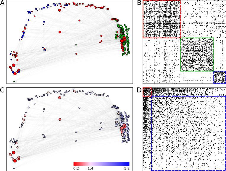
At the same time, random network models are useful for analyzing and understanding networks (Newman_2002_rg, ; leskovec2007graph, ). For example, they are routinely used as the null model to verify that features of real world networks are not due randomness (Middendorf_2005, ; Goldenberg_2010, ; Yin_2018, ) and also serve to identify community structure, as is the case with the stochastic block model and its variants (Holland_1983, ; airoldi2008mixed, ; peixoto2017bayesian, ) as well as methods such as BigCLAM (yang2013overlapping, ) and CESNA (Yang2013, ). These models successfully incorporate community structure, but have yet to effectively model core-periphery structure. While block modeling can also be used to identify core-periphery structure (Zhang_2015, ), we later show that such an approach is limited. Moreover, in general, spatial information is not often incorporated into random network models, even though it can play a large role in their structure.

Here, we present a random network model that generates networks with core-periphery structure. In our model, each vertex has a real-valued core score to reflect its role in the core. Our model assumes the edges are generated by a random process and the probability that two vertices connect is an increasing function of their core scores. Given an arbitrary network, we infer the model parameters (core scores) by maximum likelihood estimation. We prove that at any local optimum of the likelihood function, the expected degree of any node under the model is the same as the given network. Therefore, our model can be an alternative to the Chung-Lu model for generating random networks (Aiello_2001, ).

Our model also accounts for spatial locations of vertices (if such data is available). Spatial networks emerge appear in application such as trade, transportation, the power grid, and the Internet, where there is a cost associated with the length of the edges (Barthelemy_2011, ) and are known to carry core-periphery structure (Rossa_2013, ; Lee_2014, ; Dong_2015, ). In such cases, topology alone does not explain many proprieties in spatial networks, such as “small world” navigability. Our model accounts for spatial information by decreasing the probability of an edge between a pair of vertices with their distance. We show that at local optima of our likelihood function, the log of the expected geometric mean edge length of networks generated by our model is the same as in the given network from which the parameters are learned.

Spatial information enables us to design efficient algorithms for maximizing likelihood and generating random networks. The main idea is that if a set $S$ of vertices are far away in space from some given vertex $u$, then the effect of $S$ on $u$ can be efficiently approximated. We perform this approximation in a hierarchical manner similar to the fast multipole method, a “top 10 algorithm of the twentieth century” (cipra2000best, ). Although the algorithm is traditionally used to accelerate $N$-body simulations in physics, we adapt it here to develop nearly linear time algorithms for likelihood optimization and network sampling. This lets us scale to networks with millions of vertices using a commodity server.

Our model has substantially higher likelihood compared to the two other random graph models that explicitly incorporate core-periphery structure. We also show that the learned core scores are useful for downstream data mining and machine learning tasks; specifically, learned core scores out-perform existing baselines for predicting airport traffic and classifying fungal networks.

2. Model and basic inference

In this section, we develop our model for generating networks with core-periphery structure and a straightforward maximum likelihood procedure to learn model parameters for a given input network. We analyze the basic properties of the model without worrying about computation (efficient algorithms are the focus of Section 3). We provide two technical results about local optima of the likelihood function for our model: (i) the expected degree of each vertex matches the input network and (ii) the expected aggregated log-distance matches the input network.

2.1. A generative core-periphery model

Basic model.  In our basic model, we start with $n$ vertices, where each vertex $u$ has a real-valued core score $\theta_{u}$. For every pair of vertices $u$ and $v$, we add an edge between them with probability

(1) $$\textstyle\rho_{uv}=e^{\theta_{u}+\theta_{v}}\big{/}(e^{\theta_{u}+\theta_{v}}+1).$$

As a sanity check, the edge probability $\rho_{uv}\in[0,1]$ and increases monotonically as a function of the combined core score. Thus, vertices that are both “in the core” (i.e., have large core scores) are more likely to connect. Two special cases have significant meaning. First, if all vertices have the same core score $\theta_{0}$, then the model is the Erdős-Rényi model with edge probability $p=e^{2\theta_{0}}/(e^{2\theta_{0}}+1)$. Second, if the vertices are partitioned into a core $V_{c}$ with core score $\theta_{0}$ and a periphery $V_{p}$ with core score $-\theta_{0}$, then as $\theta_{0}$ increases, the model converges to a traditional block model for social networks: the core vertices $V_{c}$ form a clique while the periphery vertices $V_{p}$ form an independent set, and every pair of vertices $u\in V_{c}$ and $v\in V_{p}$ is connected with probability 0.5.

Full model.  Now we incorporate spatial information into the model. All of our subsequent algorithms and analysis are then presented for this model, which includes the basic model in Eq. 1 as a special case. Our model incorporates spatial information by adding a kernel function $K_{uv}$ to the denominator of edge probability

(2) $$\textstyle\rho_{uv}=e^{\theta_{u}+\theta_{v}}\big{/}(e^{\theta_{u}+\theta_{v}}+K_{uv}^{\epsilon}).$$

The kernel function $K_{uv}$ can be any arbitrary non-negative function provided by the user, but we mainly focus on metric kernels to study spatial networks where core-periphery structure is prevalent. We will introduce kernel functions as we go through examples, but a simple kernel is Euclidean distance: $K_{uv}=\|\bm{x}_{u}-\bm{x}_{v}\|_{2}$, where $\bm{x}_{u}$ and $\bm{x}_{v}$ are the spatial positions of vertices $u$ and $v$. We also include a tuning parameter $\epsilon$ to control the “nearsightedness” of vertices. When $\epsilon=0$, the edge probability $\rho_{uv}$ is independent of the edge length, and we recover the basic model. As $\epsilon$ increases, the fraction of long distance edges in the generated networks steeply decrease. While the parameter $\epsilon$ could be baked into the kernel, we find it useful to optimize $\epsilon$ in conjunction with the core scores $\bm{\theta}$ when fitting the model to network data (see Section 2.2).

Relationship to small worlds.  Our model is inspired in part by the Kleinberg navigable small-world model, where random edges are added to a lattice network with probability inversely proportional to powers of distance (Kleinberg_2000_navigation, ; Kleinberg_2000_algorithm, ). In real-world networks that are sparse, we expect the edge probability $\rho_{uv}$ in the corresponding generalized model to often be small. In those cases, the edge probability in our model can be approximated by

(3) $$\textstyle\rho_{uv}\approx\rho_{uv}\big{/}(1-\rho_{uv})=e^{\theta_{u}+\theta_{v}}\big{/}K_{uv}^{\epsilon}.$$

Our model thus has an interpretation for social networks: actors live somewhere in space and have different social statuses; people have a higher chance to connect if they are closer, and individuals with higher social status are likely to have more acquaintances.

2.2. Inference via Likelihood Maximization

For inference, we take as input an undirected network and a kernel function and output a set of real-valued vertex core scores and a real-valued tuning parameter $\epsilon$ for the kernel function. To do so, we maximize the log-likelihood $\Omega$:

(4) $$\textstyle\Omega=\sum_{u<v}\left[A_{uv}\log\rho_{uv}+(1-A_{uv})\log(1-\rho_{uv})\right].$$

The gradient of the edge probability with respect to the model parameters is given by simple closed-form expressions:

(5) $$\textstyle\frac{\partial\rho_{uv}}{\partial\theta_{u}}=\rho_{uv}(1-\rho_{uv}),\hskip 7.22743pt\frac{\partial\rho_{uv}}{\partial\epsilon}=-\rho_{uv}(1-\rho_{uv})\cdot\log K_{uv}.$$

First, we focus on the derivatives of the objective function with respect to the core scores:

$$\textstyle\frac{\partial\Omega}{\partial\theta_{w}} =\textstyle\sum_{u<v}\frac{\partial\rho_{uv}}{\partial\theta_{w}}\left(\frac{A_{uv}}{\rho_{uv}}-\frac{1-A_{uv}}{1-\rho_{uv}}\right)=\textstyle\sum_{u<v}(\delta_{wu}+\delta_{wv})(A_{uv}-\rho_{uv})$$

(6) $$=\textstyle\sum_{u\neq w}A_{wu}-\sum_{u\neq w}\rho_{wu}.$$

Here, $\delta_{ab}$ is the Kronecker delta function. Note that $\sum_{u\neq w}A_{wu}$ is the degree of vertex $w$ in the given network, while $\sum_{u\neq w}\rho_{wu}$ is the expected degree of vertex $w$ in the model. This observation implies our first theorem about the learned model.

Theorem 1.

At any local maximizer of the objective function $\Omega$ with respect to the core scores $\bm{\theta}$, the expected degree of every vertex in the random model equals the degree in the input network.

Next, we look at the derivative of the objective function with respect to the tuning parameter $\epsilon$,

$$\textstyle\frac{\partial\Omega}{\partial\epsilon} =\textstyle\sum_{u<v}\frac{\partial\rho_{uv}}{\partial\epsilon}\left(\frac{A_{uv}}{\rho_{uv}}-\frac{1-A_{uv}}{1-\rho_{uv}}\right)$$

$$=\textstyle-\sum_{u<v}\log K_{uv}\cdot\rho_{uv}(1-\rho_{uv})\cdot\left(\frac{A_{uv}}{\rho_{uv}}-\frac{1-A_{uv}}{1-\rho_{uv}}\right)$$

(7) $$=\textstyle-\sum_{u<v}A_{uv}\log K_{uv}+\sum_{u<v}\rho_{uv}\log K_{uv}.$$

Let $\sum_{u<v}A_{uv}\log K_{uv}$ be the aggregated log-distance, which measures the overall edge length. Then $\sum_{u<v}\rho_{uv}\log K_{uv}$ is the expected aggregated log-distance in networks generated by the learned model. This observation implies our next result.

Theorem 2.

At any local maximizer of the objective function $\Omega$ with respect to $\epsilon$, the expected aggregated log-distance in the random model equals the true aggregated log-distance in the input network.

In other words, optimizing the tuning parameter $\epsilon$ forces the overall distances in the model to match the original network.

Next, define the log geometric mean edge length (log-GMEL) of a network as

(8) $$\textstyle\textrm{log-GMEL}=\log\left[\prod_{u<v\in E}K_{uv}\right]^{\frac{1}{\lvert E\rvert}}=\frac{1}{\lvert E\rvert}\sum_{u<v\in E}\log K_{uv}$$

We argue that the log-GMEL of a random network is close to the log-GMEL of the input graph as well. By the law of large numbers, in the limit of large networks, the number of edges $\lvert E\rvert$ model concentrates around its expectation. When the number of edges is sharply concentrated about its expectation, we can approximate the expected log-GMEL by $\mathbf{E}\left[\textrm{log-GMEL}\right]\approx\mathbf{E}\left[\sum_{u<v\in E}\log K_{uv}\right]\big{/}\mathbf{E}\left[\lvert E\rvert\right]$, which is the expected aggregated log-distance divided by the expected number of edges. According to Theorems 1 and 2, the expected number of edges and the expected aggregated log-distance equal to those in the input network, respectively. Thus, the expected log-GMEL should roughly be the log-GMEL of the input network. In Section 5, we validate this numerically.

Since the derivatives of the objective function can be evaluated analytically, we use a gradient-based approach to optimize the likelihood. However, the log-likelihood objective $\Omega$ is not necessarily convex. Therefore the computed optimal set of parameters $\{\bm{\theta}^{*},\epsilon^{*}\}$ is not guaranteed to be the global maximizer of $\Omega$. Finally, even though spatial networks are our primary focus in this paper, Theorem 1 still holds for the basic model in Eq. 1. Thus, the basic model can be used for both core-periphery structure detection and as an alternative to the Chung-Lu model for generating random networks with arbitrary sequences of expected degrees.

With a naive implementation of model inference, evaluating the objective function (Eq. 4) or gradient (Eqs. 6 and 7) takes $\mathcal{O}(\lvert V\rvert^{2})$ time, regardless of the choice for the kernel function. Similarly, if we sample a random network by determining the connectivity of every pair of vertices sequentially, the overall cost is also $\mathcal{O}(\lvert V\rvert^{2})$, even if the generated network is sparse. In the next section, we design nearly linear-time approximation algorithms for both model inference and network generation when the kernel function is a metric that satisfies the triangle inequality.

3. Fast Algorithms

The quadratic scaling of the naive algorithm limits the model’s applicability to large-scale networks. In order to resolve this problem, we use a method akin to the fast multipole method (FMM) to exploit structural sparsity in the computations when the kernel is a metric, which results in nearly linear time algorithms by sacrificing a controlled amount of accuracy. The main idea of the approach is that the joint influence of a group of vertices $S$ on a far away group of vertices $T$ can be well approximated for metric kernels.

3.1. Efficient Model Inference

We will use a gradient-based method to optimize the objective function, but the computational bottleneck of optimizing model parameters is the evaluation of the objective function and its gradient. Here, we take advantage of the fact that the expressions for the objective function and its gradient are in close analogy to the gravitational potential and forces in $N$-body simulations. Similar to the gravitational potential, the objective function $\Omega$ as well as its derivative $\partial\Omega/\partial\epsilon$ consists of $\mathcal{O}(\lvert V\rvert^{2})$ pairwise interactions which decay as a function of distance (assuming a metric kernel). Furthermore, our objective function and derivative also accumulate contributions with respect to the core scores over all pairs of vertices. These similarities motivate us to use ideas from the FMM to exploit the “structural sparsity” in our computations.

Background on the FMM.  The FMM is a numerical algorithm for accelerating computation of $N$-body simulations, which require the (approximate) accumulation of $O(N^{2})$ pairwise interactions (rokhlin1985rapid, ; greengard1987fast, ). In physics, these calculations look like $P(u)=\sum_{v\in S}k(u,v)f(v)$, where $P$ is the potential (e.g., gravitational potential), $k$ is the kernel (e.g., $k(u,v)=1/\|\bm{x}_{u}-\bm{x}_{v}\|_{2}$ in gravitational potential), and $f$ is a weight function, and we want $P(u)$ for all $u\in S$. The key conceptual idea is that the interaction between two groups of well-separated particles can be well-approximated by a single interaction between the total mass of the two groups. This gives rise to the “structural sparsity” of the problem. The main mathematical idea is to use a (multipole) expansion of the kernel function to approximate these well-separated interactions (ying2012pedestrian, ; beatson1997short, ).

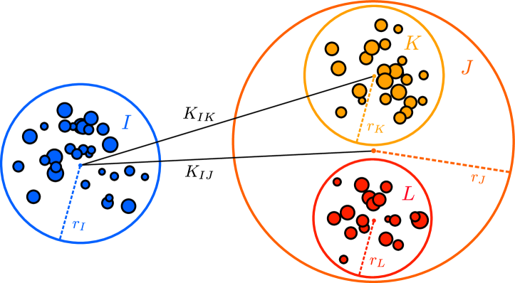
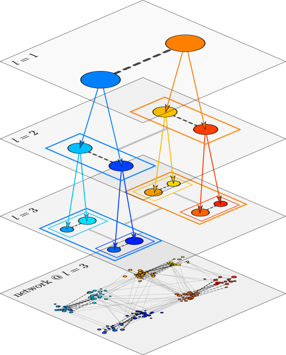
We use use a hierarchical metric-tree decomposition of the spatially distributed vertices. The root of the tree (level $l=0$) is a metric-ball containing all vertices, and we recursively bisect the network to fit into smaller metric-balls at lower levels (see Figs. 3 and 2). For example, each node at the $l=1$ level of metric-tree represents a metric-ball that encaptulates half of the vertices in the network, which is further divided into two child nodes at the $l=2$ level. Leaf nodes in the metric-tree represent a metric-ball that contains only one vertex from the network. We are using the term node to refer to metric-balls in this data structure—not to actual vertices in a network; we use vertex when referring to graphs.

Evaluating the objective function.  In order to exploit the “separation” of far-away interactions, we re-write the objective in Eq. 4 to first separate the vertex pairs that are connected:

$$\textstyle\Omega =\textstyle\sum_{u<v}\left[A_{uv}\log\rho_{uv}+(1-A_{uv})\log(1-\rho_{uv})\right]$$

$$=\textstyle\sum_{u<v\in E}\log\rho_{uv}+\sum_{u<v\not\in E}\log(1-\rho_{uv})$$

$$=\textstyle\sum_{u<v\in E}\log\frac{\rho_{uv}}{(1-\rho_{uv})}-\sum_{u<v}\log(1+e^{\theta_{u}+\theta_{v}}\big{/}K_{uv}^{\epsilon}).$$

Recall from Theorem 1 that at any local maximizer of the objective function, the expected degree of a vertex in the model equals its degree in the given network (i.e., $\sum_{u\neq w}\rho_{wu}=\sum_{u\neq w}A_{wu}$). If the given network is sparse, then $\sum_{u\neq w}A_{wu}\ll\lvert V\rvert$ holds for most vertices, $\rho_{uv}\ll 1$ holds for most vertex pairs, and $z_{uv}\equiv e^{\theta_{u}+\theta_{v}}\big{/}K_{uv}^{\epsilon}=\rho_{uv}\big{/}(1-\rho_{uv})\ll 1$. In other words, the learned core scores in the given network are small enough that $e^{\theta_{u}+\theta_{v}}\ll K_{uv}$ for most pairs of vertices. Thus, we can use the Maclaurin expansion for $\log(1+z_{uv})$ to approximate the objective function,

$$\textstyle\Omega\approx\sum_{u<v\in E}\log\frac{\rho_{uv}}{1-\rho_{uv}}-\sum_{u<v}\sum_{t=1}^{T}\frac{(-1)^{t-1}}{t}\left(\frac{e^{\theta_{u}+\theta_{v}}}{K_{uv}^{\epsilon}}\right)^{t}.$$

Here, $T$ is a small constant ($T=4$ in our implementation; larger expansions provided little benefit in accuracy). The first term in the expansion only sums over connected vertex pairs and can be calculated in $\mathcal{O}(\lvert E\rvert)$ time. The summation over the $\mathcal{O}(\lvert V\rvert^{2})$ pairwise interactions in the second term of the expansion is accelerated by grouping vetices in the same metric-ball and computing interactions between two groups of vertices at once. While we have made several approximations in our arguments, our numerical experiments in Section 4.1 show that they are valid on real-world networks.

Our FMM-like implementation is similar to the algorithm presented in the original literature known as the “tree-code” (Apple_1985, ). At each level $l$ of the metric-tree, for every pair of sibling metric-balls $I,J$, we sum over the interaction between every pair of vertices with one end in $I$ and the other in $J$,

(9) $$\textstyle\sum_{u<v}\left(\frac{e^{\theta_{u}+\theta_{v}}}{K_{uv}^{\epsilon}}\right)^{t}=\sum_{l}\sum_{\begin{subarray}{c}I<J\in B_{l}\\ p(I)=p(J)\end{subarray}}\left[\sum_{u\in I,v\in J}\left(\frac{e^{\theta_{u}+\theta_{v}}}{K_{uv}^{\epsilon}}\right)^{t}\right],$$

where $B_{l}$ represents the set of metric-balls at level $l$ of the metric-tree, and $p(I),p(J)$ denote the parent metric-balls of $I,J$ respectively.

In order to guarantee the accuracy of the FMM algorithm, the pairwise interactions between vertices in $I$ and $J$ (in the square bracket of Eq. 9) can only be computed at once if the separation between the metric-balls is large relative to their radii, i.e.,

(10) $$\textstyle K_{IJ}\big{/}(r_{I}+r_{J})>\delta_{1},$$

where $r_{I},r_{J}$ are the radii of the metric-balls, $K_{IJ}$ measures the metric distance between their centers of mass, and $\delta_{1}$ is a user-input accuracy. For our problem, we also have to make sure the assumption $z_{uv}\ll 1$ holds for every pair of vertices with one end in $I$ and the other in $J$, i.e.,

(11) $$\textstyle e^{\max\{\theta_{u}\;|\;u\in I\}}\cdot e^{\max\{\theta_{v}\;|\;v\in J\}}/K_{IJ}<\delta_{2},$$

where $\delta_{2}$ is another user-input accuracy parameter. We use $\delta_{1}=2.0$ and $\delta_{2}=0.2$ as default in our implementation. However, the user can tune these parameters to trade off accuracy and computation time (we conduct trade-off experiments in Section 4.1).

If the two accuracy criteria in Eq. 10 and Eq. 11 are satisfied, then the long-range pairwise interactions between $I$ and $J$ can be approximated as follows:

(12) $$\textstyle\sum_{u\in I,v\in J}\left(\frac{e^{\theta_{u}+\theta_{v}}}{K_{uv}^{\epsilon}}\right)^{t}\approx\left(\sum_{u\in I}e^{\theta_{u}}\right)^{t}\left(\sum_{v\in J}e^{\theta_{v}}\right)^{t}\big{/}K_{IJ}^{t\epsilon}.$$

On the other hand, if one or more accuracy criteria are not satisfied, then without loss of generality, $I$ is the metric-ball with smaller radius ($r_{I}<r_{J}$), and we compute the interactions between metric-ball $I$ and each of the two child metric-balls of $J$ separately (Fig. 2). The exact computational complexity of the FMM algorithm depends on the parameters $\delta_{1}$ and $\delta_{2}$. In practice, the objective function is approximated to within $1\%$ error using the default parameters (see Section 4.1), and the overall time complexity is $\mathcal{O}(\lvert E\rvert+\lvert V\rvert\log\lvert V\rvert)$.

Figure 2. Interactions between vertices in $I$ and $J$ with our algorithm. If the accuracy criteria in Eqs. 10 and 11 are satisfied, then we approximate the interaction between all vertices in $I$ and all vertices in $J$ with a single point in each ball (Eq. 12). Otherwise, we recurse and consider the interactions between $I$ and $K$ as well as $I$ and $L$.

Evaluating the gradient.  We can also use the FMM to approximate the derivative of $\Omega$ with respect to the core score $\theta_{w}$. At each level $l$ of the metric tree, we sum over the interactions between vertex $w$ and all the vertices in the metric-ball $J_{l}$ which is the sibling to the metric-ball $I_{l}$ that contains $w$,

$$\textstyle\frac{\partial\Omega}{\partial\theta_{w}} =\textstyle\sum_{u\neq w}A_{wu}-\sum_{u\neq w}e^{\theta_{u}+\theta_{w}}\big{/}\left[e^{\theta_{u}+\theta_{w}}+K_{uw}^{\epsilon}\right]$$

$$=\textstyle\sum_{u\neq w}A_{wu}-\sum_{l}\sum_{u\in J_{l}}e^{\theta_{u}+\theta_{w}}\big{/}\left[e^{\theta_{u}+\theta_{w}}+K_{uw}^{\epsilon}\right]$$

(13) $$\textstyle\approx\sum_{u\neq w}A_{wu}-e^{\theta_{w}}\sum_{l,u\in J_{l}}e^{\theta_{u}}\big{/}\left[\frac{e^{\theta_{w}}}{\lvert J_{l}\rvert}\sum_{u\in J_{l}}e^{\theta_{u}}+K_{I_{l}J_{l}}^{\epsilon}\right].$$

The first term of Eq. 13 is the degree of vertex $w$, which can be evaluated upfront in $\mathcal{O}(\lvert E\rvert)$ time. Moreover, if we precompute and store $\sum_{u\in J_{l}}e^{\theta_{u}}$ for all metric-balls, then the second term can be computed in $\mathcal{O}(\lvert V\rvert\log\lvert V\rvert)$ time. Therefore, the overall cost of evaluating the core score derivatives for all the vertices is $\mathcal{O}(\lvert V\rvert\log\lvert V\rvert+\lvert E\rvert)$. Furthermore, we can also approximate the derivative of the objective function with respect to $\epsilon$:

$$\textstyle\frac{\partial\Omega}{\partial\epsilon} =\textstyle\sum_{u<v\in E}-\log K_{uv}+\sum_{u<v}\frac{e^{\theta_{u}+\theta_{v}}\log K_{uv}}{e^{\theta_{u}+\theta_{v}}+K_{uv}^{\epsilon}}$$

$$\textstyle\sum_{u<v\in E}-\log K_{uv}+\sum_{l}\sum_{\begin{subarray}{c}I<J\in B_{l}\\ p(I)=p(J)\end{subarray}}\sum_{u\in I,v\in J}\frac{e^{\theta_{u}+\theta_{v}}\log K_{uv}}{e^{\theta_{u}+\theta_{v}}+K_{uv}^{\epsilon}}.$$

The first term in the last equation can be calculated in $\mathcal{O}(\lvert E\rvert)$ time, while the second term can be evaluated in $\mathcal{O}(\lvert V\rvert\log\lvert V\rvert)$ following the same scheme as the objective function,

(14) $$\sum_{\begin{subarray}{c}u\in I\\ v\in J\end{subarray}}\frac{e^{\theta_{u}+\theta_{v}}\log K_{uv}}{e^{\theta_{u}+\theta_{v}}+K_{uv}^{\epsilon}}\approx\frac{\sum_{u\in I}e^{\theta_{u}}\cdot\sum_{v\in J}e^{\theta_{v}}\cdot\log K_{IJ}}{\frac{1}{\lvert I\rvert}\sum_{u\in I}e^{\theta_{u}}\cdot\frac{1}{\lvert J\rvert}\sum_{v\in J}e^{\theta_{v}}+K_{IJ}^{\epsilon}}.$$

Unlike the FMM-style approximation for the objective function (Eq. 12), the denominators in the expression of the objective function gradient (Eqs. 13 and 14) are not metric kernels due to the extra terms that involve the vertex core scores. However, when the given network is sparse and the fitted core scores are small, the metric kernels $K_{I_{l}J_{l}}^{\epsilon}$ and $K_{IJ}^{\epsilon}$ dominate the denominators of Eq. 13 and Eq. 14, making them good approximations for metric kernels.

The FMM-style algorithm enables efficient model inference, and the learned core scores are accurate enough for data mining purposes, which we show in Section 5. Furthermore, we also want to generate random spatial networks, which naively takes $\mathcal{O}(\lvert V\rvert^{2})$ time. We show how to accelerate this process in the next section.

Figure 3. The top three levels in the metric-tree data structure. Each circle in the diagram represents a metric-ball that encapsulates spatially adjacent vertices. This data structure is used for efficient evaluation of the objective function and its gradient as well as for efficient network generation. For objective function evaluation, the dashed lines at each layer of the diagram represent the pairwise interactions accumulated at the corresponding level of the metric-tree. For random network generation, the dashed lines represent the edges sampled at each level of the metric-tree between sibling metric-balls, while the solid lines represent edges that are already generated in previous levels. The bottom layer of the diagram shows the random network generated at the $l=3$ level of the metric tree; edges between vertices within the same metric ball at this level are not yet considered.

3.2. Efficient Random Network Generation

Given the core scores, we can naively sample a random networks by flipping a biased coin for each pair of vertices. However, this process is inefficient when the output network is sparse. To address this problem, we develop an efficient algorithm to hierarchically sample the edges. The key idea is to sample edges between pairs of metric-balls instead of pairs of vertices.

Our algorithm proceeds as follows. First, we recursively partition the vertices to fit into a metric-tree. Second, at each level of the tree, for every pair of sibling metric-balls $I,J$, we compute the expected number of edges $n_{IJ}$ that has one end in each of $I$ and $J$:

(15) $$n_{IJ}\approx\frac{\sum_{u\in I}e^{\theta_{u}}\cdot\sum_{v\in J}e^{\theta_{v}}}{\frac{1}{\lvert I\rvert}\sum_{u\in I}e^{\theta_{u}}\cdot\frac{1}{\lvert J\rvert}\sum_{v\in J}e^{\theta_{v}}+K_{IJ}^{\epsilon}}.$$

Third, we determine the edges between every pair of sibling metric-balls $I,J$ by sampling $n_{IJ}$ vertices independently from $I$ with probability $\rho_{u}\propto e^{\theta_{u}}\big{/}\left[\frac{e^{\theta_{u}}}{\lvert J\rvert}\sum_{v\in J}e^{\theta_{v}}+K_{IJ}^{\epsilon}\right]$, and $n_{IJ}$ vertices independently from $J$ with probability $\rho_{v}\propto e^{\theta_{v}}\big{/}\left[\frac{e^{\theta_{v}}}{\lvert I\rvert}\sum_{u\in I}e^{\theta_{u}}+K_{IJ}^{\epsilon}\right]$. Finally, we pair samples from $I$ and $J$ sequentially. The cost for sampling vertices with non-uniform probability in the third step is $\mathcal{O}(\lvert I\rvert+\lvert J\rvert+n_{IJ}\log n_{IJ})$. Assuming the generated network is sparse and the number of edges grows linearly with the number of vertices ($n_{IJ}\propto\lvert I\rvert+\lvert J\rvert$), the overall cost is $\mathcal{O}\left(\lvert V\rvert(\log\lvert V\rvert)^{2}\right)$.

Creating edges by pairing up independently sampled vertices is called “ball-dropping” in Erdős-Rényi sampling (Ramani_2017, ). In our model, the number of edges between metric-balls $I$ and $J$ does not have a closed-formed probability distribution, and our algorithm is only taking the mean of that distribution by sampling $n_{IJ}$ edges. Therefore, our fast sampling scheme is only an approximation without any theoretical guarantees. However, as we show in the next section, this approximation empirically preserves network properties.

4. Methodological experiments

In this section, we first numerically validate our approximations and then show that our model achieves much higher likelihood than competing generative models for core-periphery structure. Section 5 then explores data mining tasks aided by our model.

4.1. Approximation validation

In the previous section, we made a number of approximations in our methods. We now show that these approximations indeed have small error. To optimize the objective function, we use the limited-memory BFGS (L-BFGS) algorithm from the Optim.jl package (Mogensen_2018, ). We also use a diagonal preconditioner in case the approximated Hessian used within L-BFGS becomes ill-conditioned. We construct the metric-tree with the NearestNeighbors.jl package. Finally, we set the tolerance parameters to $\delta_{1}=2.0$ and $\delta_{2}=0.2$.

Figure 4. (A) Agreement between the naive (blue) and fast (orange) algorithms on the expected vertex degrees. The error of the FMM-style approximation is in red. We also include the vertex degrees in the original network (gray) as numerical validation for Theorem 1. (B) Correlation between the learned core scores from the naive algorithm and the FMM algorithm. The Pearson correlation coefficient is 0.999.

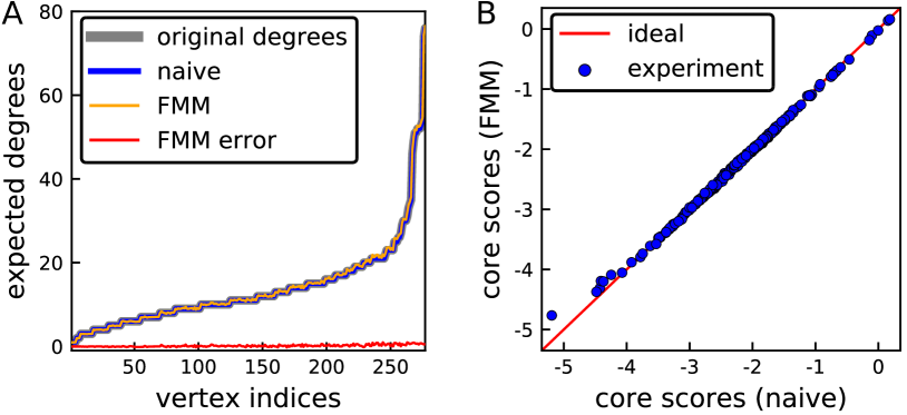
Accuracy in evaluating the objective function and derivative.  To test our fast algorithm, we first learn parameters for the C. elegans network from Fig. 1 using the naive algorithm and the Euclidean distance kernel. Next, we evaluate $\Omega$ and the gradient using the same parameters, but this time using the fast algorithm to sum over the pairwise interactions between vertices. The relative difference in $\Omega$ between the naive and the fast algorithms was less than 1%. To evalualuate agreement in the derivative, we compare expected degrees obtained by the fast algorithm and the naive algorithm and find them to be nearly identical (Fig. 4). As a sanity check, the expected vertex degrees computed by both algorithms are very close to the vertex degrees in the original network, which is a necessary condition for $\Omega$ to be at a local maximum (Theorem 1).

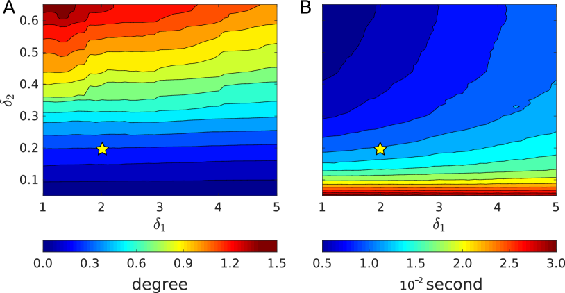
To understand how the quality of the approximation depends on the input accuracy parameters, we repeat the above experiments using different combinations of $\delta_{1}$ and $\delta_{2}$. We characterize the approximation error with the root mean square error in expected degrees between the fast algorithm and the naive algorithm (Fig. 6) and report dependence of the running time on the accuracy parameters (Fig. 6). Both accuracy and running time have a stronger dependency on $\delta_{2}$ as compared to $\delta_{1}$. This reason is that when our algorithm determines the radius of the parent metric-ball, it assumes the worst-case condition and chooses a large value. Therefore in most cases, $\delta_{1}=1.0$ could already guarantee that all the vertices between two metric-balls are well-separated.

Next, we use our fast algorithm to learn the model parameters. The learned vertex core scores with the naive and the fast algorithms had Pearson correlation of $0.999$ and empirically look similar (Fig. 4). Furthermore, the learned $\epsilon$ by the naive algorithm and the FMM algorithm were $0.499$ and $0.506$, respectively.

Figure 5. Performance dependence on accuracy parameters on the C. elegans network. The yellow stars represent the location of default parameters. (A) Root mean square error in expected degrees. (B) Running time per gradient evaluation.

Figure 6. (A) Correlation of vertex degrees in C. elegans and the random networks generated by the naive and fast algorithm; the Pearson correlation coefficients are 0.983 and 0.981, respectively. (B) Number of edges whose kernel distance is below a distance threshold. The agreement numerically validates our fast sampling algorithm as well as our arguments in Section 3 on preserving distances.

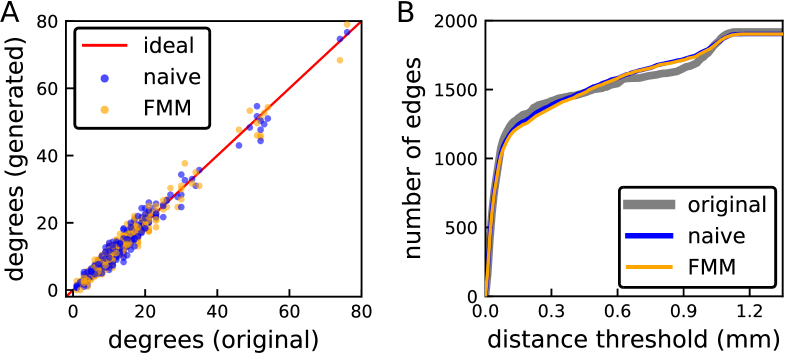
Quality of generated random networks.  Using the model parameters learned by the naive algorithm, we now confirm that random networks generated by the naive sampling algorithm and the fast sampling algorithm are similar. We first consider the degree distribution. For both the naive algorithm and the fast algorithms, we compare the mean degrees over three sampled networks to the degree in the original network (Fig. 6). Indeed, the degrees in the random networks generated by both algorithms are highly correlated with that in the original network.

Next, we consider the edge length distribution given by the kernel function. We argued that the expected log-GMEL in the generated random networks equals that in the original network at any local maximum of the likelihood function. Indeed, the GMEL in C. elegans is $0.079$mm, while the GMEL in the random networks generated by the naive algorithm and the fast algorithm (averaged over three samples) are $0.078$mm and $0.079$mm. For a more detailed analysis, we picked equispaced distance thresholds from $0.0$mm to $1.4$mm and counted the number of edges in the network whose length is smaller than each threshold. The counts of the original network, the mean of three naive random samples, and the mean of three samples with our fast algorithm are nearly identical (Fig. 6).

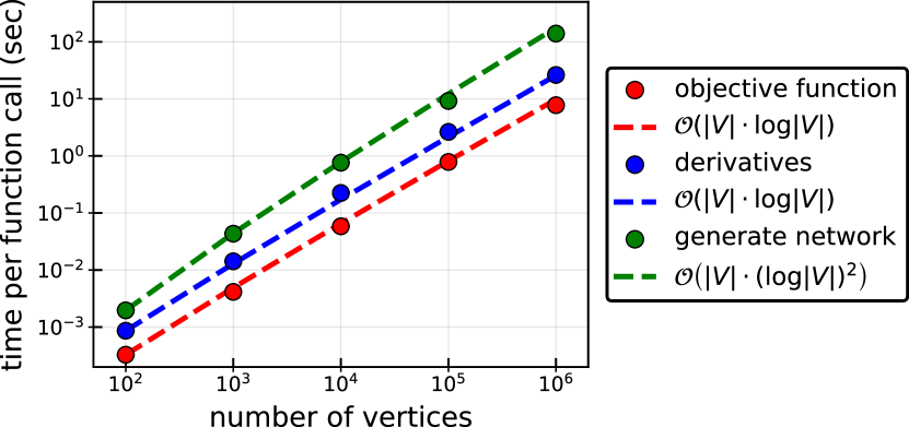
Scalability of the FMM-style algorithm.  Finally, we validate the computational complexity of our proposed methods. We run our algorithms on synthetic 2-block core-periphery networks where vertex coordinates are randomly generated in the 2-dimensional unit square. We choose 5% of the vertices in the networks as the core, and their core score (denoted as $\theta_{c}$) is set to be $1.0$ unit larger than the core score of the periphery vertices (denoted as $\theta_{p}$). The core scores $\theta_{c},\theta_{p}$ in this family of networks are chosen so that the number of edges grows linearly with the number of vertices (in the five networks, $\theta_{c}=$ $-1.25$, $-2.77$, $-4.13$, $-5.43$, $-6.69$). Fig. 7 shows that the empirical running time follows the theoretical analysis.

Figure 7. Scalability of our FMM-style algorithms using synthetic networks, where the average degree in each network is 10. Observed timings are scattered with circles, and ideal efficiencies are plotted in dashed lines.

4.2. Likelihood comparison

We now demonstrate the quality of our model by comparing its optimized log-likelihood with the only other two generative models for core-periphery structure. The first is a 2-block stochastic block model with a belief propagation learning algorithm that explicitly incorporates core-periphery structure (henceforth, SBM-CP) (Zhang_2015, ). Since the belief propagation algorithm is sensitive to the initial conditions, we perform $5$ independent runs of the algorithm from different random initial conditions and record the best result. The second model defines the edge probability as a logistic function of the “centrality rank” of the incident vertices (henceforth, logistic-CP) (Tudisco_2018, ). For this model, we tune the hyperparameters $s,t$ in the logistic function with grid search and record the best result.

Table 1. Number of nodes ($n$), number of edges ($m$), and optimized log-likelihood of our model, SBM-CP and logistic-CP. In all datasets, our model has a larger likelihood. (Results for logistic-CP are only available for connected graphs.)

			Log likelihood
Dataset	$n$	$m$	our model	SBM-CP	logistic-CP
C. elegans	279	1.9K	-$6.3\cdot 10^{3}$	$-7.1\cdot 10^{3}$	$-7.0\cdot 10^{3}$
London Under.	315	370	$-6.0\cdot 10^{2}$	$-2.2\cdot 10^{3}$	$-2.1\cdot 10^{3}$
Pv_M_I_U_N_42d_1	2.4k	2.6K	$-6.4\cdot 10^{3}$	$-2.1\cdot 10^{4}$	—
OpenFlights	7.2K	18.6K	$-4.7\cdot 10^{4}$	$-1.1\cdot 10^{5}$	—
Brightkite	50.7K	194K	$-1.3\cdot 10^{6}$	$-1.9\cdot 10^{6}$	—
LiveJournal	1.16M	7.19M	$-7.5\cdot 10^{7}$	$-8.9\cdot 10^{7}$	—

We learn the parameters of our model, SBM-CP and logistic-CP on six datasets (basic summary statistics are listed in Table 1):
(i) The neural network of the nematode worm C. elegans from Fig. 1.
(ii) The network of the London underground transportation system, where vertices are tube stations and edges connect stations.
(iii) The fungal network Pv_M_I_U_N_42d_1 constructed from a laboratory experiment, where each hypha (tubular cell) is a vertex, and each cord transporting nutrients between two hyphae is an edge (Lee_2017, ). The fungus grows on a 2-dimensional plane.
(iv) The airline transportation network from OpenFlights. Vertices are airports with latitude and longitude spatial locations, and edges correspond to available direct flights.
(v) The Brightkite social network (cho2011friendship, ). Vertices are users and spatial locations come from the user’s most recent check-in.
(vi) The LiveJournal social network (Liben-Nowell_2005, ). Vertices are bloggers and the spatial locations are given by the city listed in the user’s profile. Edges are friendships listed in a user’s profile.

A small amount of noise was added to locations in the Brightkite and LiveJournal datasets to avoid having vertices in the same location. For the OpenFlights, Brightkite, and LiveJournal datasets, spatial positions are latitude and longitude, so we use the great circle distance kernel. For C. elegans and the fungal network, we use Euclidean distance. In the London Underground dataset, tube stations are almost always connected to their closest spatial neighbors due to construction cost of railways. Therefore, we choose a symmetric version of rank distance (Liben-Nowell_2005, ) as the kernel. Table 1 lists the optimized log-likelihoods of our model, SBM-CP and logistic-CP; our model always has substantially higher likelihood.

5. Data mining experiments

Now that we have addressed the accuracy, scalability, and efficacy of our algorithms and model, we use the output of our model to study real-world spatial networks. We find that the learned core scores from our model are good predictors for traffic in an airport network and for the classification of fungal networks.

5.1. Case study I: Predicting enplanement

We first analyze the OpenFlights network introduced in Section 4.2. Recall that this network has vertices representing airports and edges representing direct flights between airports. Given the network and vertex coordinates, our goal is to predict the total number of passengers boarding (enplanement) at each airport in the year 2017 using vertex core scores. To this end, we first compute the vertex core scores using the FMM-style algorithm with the great-circle distance kernel (Fig. 8) and then we use a decision tree to correlate the vertex core scores with enplanement (Fig. 9)

Figure 8. Vertex core scores in the airline network. The top 10% of the vertices with highest core scores are colored in orange, while the rest are colored in blue. The radius of a vertex is proportional to the square root of its degree.

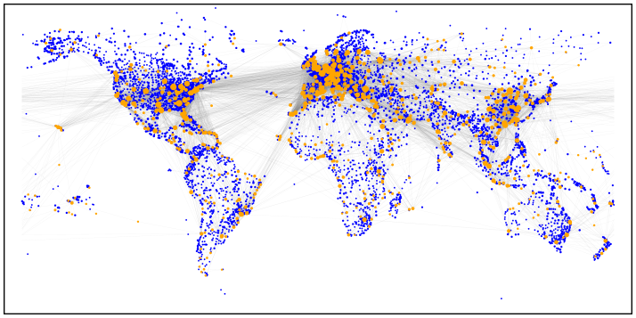
We obtained the enplanement metadata for $447$ airports in the United States. We first split the airports randomly into a training set of $357$ airports ($80\%$) and test set of $90$ airports ($20\%$); after, we build a decision tree using the training set and test its prediction accuracy on the testing set. Figure 9 shows an instance of the decision tree we build using the training set.

Figure 9. Top three levels of the decision tree for predicting airport enplanement using vertex core scores. The leaf nodes in the decision tree is the average enplanement (in millions) among airports with core scores in the given range.

We average the prediction accuracy of decision trees over $10$ random split of the training and testing set, and the mean coefficient of determination ($R^{2}$) between ground truth and predicted enplanement is $0.846$. Analogous experiments are repeated using vertex degrees, betweenness centrality (BC) (Freeman_1977, ), closeness centrality (CC) (Bavelas_1950, ), eigenvector centrality (EC) (Newman_2003, ) or PageRank (PR) (Pageetal_1998, ) instead of the core score as the independent variable (Table 2). The vertex core scores outperforms other centrality measures in characterizing airport enplanement. This high accuracy indicates that our model effectively utilizes spatial information.

Table 2. The $R^{2}$ values between ground truth and predicted enplanement with different features. Our learned core scores have the largest value.

	degree	BC	CC	EC	PR	core score
$R^{2}$	$0.762$	$0.293$	$0.663$	$0.542$	$0.637$	0.846

5.2. Case study II: Classifying fungal networks

In this case study, we use core scores to predict types of fungal networks (the network examined in Section 4.2 is one such network). In these networks, vertices are hyphae in 2-dimensional Euclidean space and edges are cords transporting nutrients between two hyphae. Based on the species and growing conditions, the fungal networks were categorized into $15$ different classes (Lee_2017, ). Here, we use core scores as features to predict the class label of each network.

First, we learned the vertex core scores for every fungal network using our model with the Euclidean distance kernel and the FMM-style algorithm. Then, for each network, we created a 4-element feature vector using the maximum, mean, and standard deviation of the core scores, along with the number of vertices. We trained a logistic regression model with these features (and an intercept term) and evaluated prediction accuracy with 5-fold cross validation. We repeated the experiment using the centrality measures from Section 5.1. Table 3 shows that core scores from our model are the best predictors. As evidence for why this might be true, Fig. 10 plots the mean and maximal core score for each network, along with the class labels. We see class separation with these two features.

Figure 10. Maximal and mean vertex core scores for 260 fungal networks. The integer in the parentheses after each class label is the number of networks in that class. The plot shows some clustering of class type based on these features. We use these features along with a couple others derived from the learned core scores to train a logistic regression classifier with good performance (Table 3).

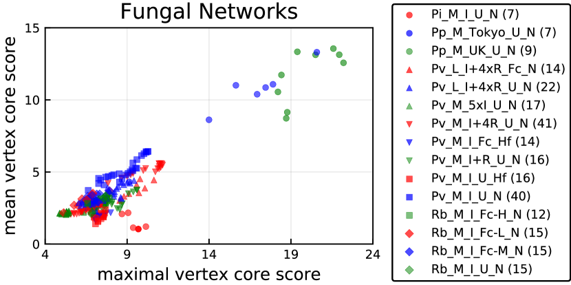
Furthermore, we use a logistic regression model by concatenating information from vertex degrees and core scores as features. In other words, the predictors are the maximum, mean and standard deviation of vertex degrees; the maximum, mean, and standard deviation of vertex core scores; and the number of vertices. We observe a large increase in prediction accuracy from $43.5\%$ to $65.6\%$. This result shows that vertex core scores captures different information than degrees in the fungal networks.

Table 3. Cross validation accuracy of fungal networks classification using different features. Our learned core scores give the best prediction. “Random” is random guessing.

random	degree	BC	CC	EC	PR	core score
6.7%	38.0%	23.7%	19.0%	20.2%	18.6%	43.5%

6. Additional related work

The idea of core-periphery structure has a long history in the theory of social networks (Burt-1976-Positions, ; Breiger-1981-structures, ; Borgatti_2000, ), where the core arises due to differential status. Borgatti and Everett developed the first significant computational approach to identify core-periphery structure (Borgatti_2000, ). Since then, several methods have been deisgned to find core-periphery structure, based on paths (Lee_2014, ; Gamble_2016, ), vertex covers (benson2018found, ), spectral information (Cucuringu_2016, ; Ma_2018, ), $k$-cores and generalizations (dumba2018uncovering, ; sariyuce2015finding, ), hand-crafted “core quality” objective functions (Rombach-2014-CP, ; Rombach_2017, ; Kojaku_2018, ), and user studies (joblin2017classifying, ). Such methods are typically analyzed via synthetic benchmarks, density measures, or network visualizations. The key difference with our work is that we propose a generative model, whereas prior work performs post hoc identification of core-periphery structure using the network topology. The only other generative models are due to Zhang et al. (Zhang_2015, ) and Tudisco and Higham (Tudisco_2018, ) against which we compared in Section 4.2 (unlike our approach, these methods do not use spatial information).

Network centrality captures similar properties to core-periphery structure. Indeed, closeness centrality is used to detect core vertices in networks (Holme_2005, ; Silva_2008, ), and centrality measures are baselines for core-periphery identification measures (Rombach_2017, ) (see also our experiments in Section 5). A subtlety is that network centrality can be a consequence of core-periphery dynamics, but centrality in and of itself does not lead to a reason for core-periphery structure. This is one reason why we developed a generative model in this paper.

7. Discussion

We have developed a random network model for core-periphery structure, where each vertex has a real-valued core score. We focused our analysis on spatial data, which connects to the small-world model where edge probabilities are inversely correlated with distance. The spatial structure enabled us to develop fast algorithms for both gradient-based inference and network sampling. We showed both theoretically and numerically that our model preserves the expected degree of each vertex as well as the aggregated log-distance. Our model can be an alternative to the Chung-Lu model, even if there is no spatial metadata. Furthermore, our model does not need to learn from a network—given a prescribed set of core scores and a kernel function, we can generate networks.

In terms of likelihood, our model out-performs the only other generative models for core-periphery structure (SBM-CP and logistic-CP). The basic version of our model can be thought of as a continuous relaxation of SBM-CP, since the core scores permit a continuum of edge probabilities. Finally, we also demonstrated that the learned core scores are useful vertex features for downstream network analysis and machine learning tasks in two very different complex systems (airport traffic and fungal growth), which provides evidence that our model could be incorporated into a wide area of application domains.