Study of Set-Membership Adaptive Kernel Algorithms

André Flores and Rodrigo C. de Lamare André Flores is with the Centre for Telecommunications Studies (CETUC), PUC-Rio, Rio de Janeiro, Brazil and Rodrigo C. de Lamare is with both CETUC and with the Department of Electronic Engineering, University of York, UK. Part of this work has been presented at the IEEE International Conference on Acoustics, Speech and Signal Processing 2017. The emails of the authors are andre.flores@cetuc.puc-rio.br and delamare@cetuc.puc-rio.br
Abstract

In the last decade, a considerable research effort has been devoted to developing adaptive algorithms based on kernel functions. One of the main features of these algorithms is that they form a family of universal approximation techniques, solving problems with nonlinearities elegantly. In this paper, we present data-selective adaptive kernel normalized least-mean square (KNLMS) algorithms that can increase their learning rate and reduce their computational complexity. In fact, these methods deal with kernel expansions, creating a growing structure also known as the dictionary, whose size depends on the number of observations and their innovation. The algorithms described herein use an adaptive step-size to accelerate the learning and can offer an excellent tradeoff between convergence speed and steady state, which allows them to solve nonlinear filtering and estimation problems with a large number of parameters without requiring a large computational cost. The data-selective update scheme also limits the number of operations performed and the size of the dictionary created by the kernel expansion, saving computational resources and dealing with one of the major problems of kernel adaptive algorithms. A statistical analysis is carried out along with a computational complexity analysis of the proposed algorithms. Simulations show that the proposed KNLMS algorithms outperform existing algorithms in examples of nonlinear system identification and prediction of a time series originating from a nonlinear difference equation.

Keywords:
Adaptive algorithms, set-membership algorithms, data-selective techniques, kernel methods, statistical analysis.

I Introduction

Adaptive filtering algorithms have been the focus of a great deal of research in the past decades and the machine learning community has embraced and further advanced the study of these methods. In fact, adaptive algorithms are often considered with linear structures, which limits their performance and does not draw attention to nonlinear problems that can be solved in various applications. In order to deal with nonlinear problems a family of nonlinear adaptive algorithms based on kernels has been developed. In particular, a kernel is a function that compares the similarity between two inputs and can be used for filtering, estimation and classification tasks. Kernel adaptive filtering (KAF) algorithms have been tested in many different scenarios and applications [1, 2, 3, 4, 5], showing very good results. One of the main advantages of KAF algorithms is that they are universal approximators [1], which gives them the ability to address complex and nonlinear problems. However, their computational complexity is much higher than their linear counterparts [1].

One of the first KAF algorithms to appear, which is widely adopted in the KAF family because of its simplicity, is the kernel least-mean square (KLMS) algorithm proposed in [6] and later extended in [7]. The KLMS algorithm has been inspired by the least-mean square (LMS) algorithm and, thanks to its good performance, led many researchers to work in the development of kernel versions of conventional adaptive algorithms. For instance, a kernel version of the NLMS algorithm has been proposed in [5] using a nonlinear regression approach for time series prediction. In [8, 9], the affine projection algorithm (APA) has been used as the basis of the derivation of kernel affine projection (KAP) algorithms. Adaptive projection algorithms using kernel techniques have been reported in [10, 11]. The recursive least squares algorithm (RLS) has been extended in [12], where the kernel recursive least squares (KRLS) has been described. Later, the authors of [13] proposed an extension of the KRLS algorithm and the use of multiple kernels has been studied in [14] and [15].

Previously reported kernel algorithms have to deal with kernel expansions, which increases significantly the computational cost. In other words, they create a growing structure, also called dictionary, where every new data input that arrives is employed to compute the estimate of the desired output. The natural problem that arises is that the time and computational cost required to compute a certain output could exceed the tolerable limits for an application. Several criteria to manage the growing structure of kernel algorithms have been proposed to solve this problem such as algorithms with fixed dictionary size as studied in [16, 17] and [18]. One of the most simple criteria is the novelty criterion (NC), presented in [19]. Specifically, NC establishes two thresholds to limit the size of the dictionary. Another method, the approximate linear dependency (ALD) has been proposed in [12] and verifies if a new input can be expressed as a linear combination of the elements stored before adding this input to the dictionary. The coherence criterion (CC) has been described in [5] also to limit the size of the dictionary based on the similarity of the inputs. A measure called surprise criterion (SC) has been presented in [20] to remove redundant data.

In this work, we present set-membership normalized kernel least-mean square (SM-KNLMS) adaptive algorithms, which have been initially reported in [21, 22] and can provide a faster learning than existing kernel-based algorithms and limit the size of the dictionary without compromising performance. Unlike the equivalent set-theoretic approach in [11] the set-membership algorithms presented here exploit variable step sizes, which can lead to a faster learning performance. Similarly to existing set-membership algorithms [23, 24, 25, 26, 27, 28, 29, 30], the proposed SM-KNLMS algorithms are equipped with variable step sizes and perform sparse updates. We consider both centroid-based SM-KNLMS (C-SM-KNLMS) and nonlinear regression-based SM-KNLMS (NLR-KNLMS) algorithms, where the latter lends itself to statistical analysis [5]. Unlike existing kernel-based adaptive algorithms the proposed SM-KNLMS algorithms deal, in a natural way, with the kernel expansion because of the data selectivity based on error bounds that they implement. A statistical analysis of the NLR-SM-KNLMS algorithm along with the derivation of analytical formulas to predict the mean-square error (MSE), and an analysis of their computational cost are carried out. Simulations comparing the performance of the SM-KNLMS and existing algorithms for several scenarios are then conducted.

In summary, the contributions of this work are:

  • The development of the proposed C-SM-KNLMS and NLR-SM-KNLMS algorithms.

  • A statistical analysis of the NLR-SM-KNLMS algorithm and the development of analytical formulas to predict its performance.

  • A simulation study of the proposed C-SM-KNLMS, NLR-SM-KNLMS and existing algorithms for several scenarios of interest.

This paper is organized as follows. In Section II, the principles of kernel methods and set-membership techniques are introduced. In Section III, we review set-membership adaptive algorithms and present the derivation of the proposed C-SM-KNLMS algorithm. Section IV presents the proposed NLR-SM-KNLMS algorithm. Section V details the statistical analysis of the NLR-SM-KNLMS algorithm and a comparison of the computational complexity of the proposed and existing algorithms. Section VI describes and discusses the simulation results and Section VII contains the conclusions of this work.

II Principles of Kernel Methods and Set-Membership Techniques

Conventional adaptive algorithms work with linear structures, limiting the performance that they can achieve and constraining the number of problems that can be solved. Under this scope, a new family of nonlinear adaptive algorithms based on kernels has been developed [1]. The main objective of these algorithms is to learn an arbitrary input-output mapping based on a sequence of samples and a kernel. Basically, a kernel κ(,)𝜅\kappa\left(\cdot,\cdot\right) is a function that measures the similarity between two inputs and generally returns a real number. Several kernel functions are described in the literature [1]. Choosing a kernel function is important because it is equivalent to implicitly defining a feature space where the algorithms are performed. Let us now introduce two commonly used kernel functions. The first one is the Gaussian kernel, defined by

κ(𝐱,𝐱)=exp(𝐱𝐱22ν2),𝜅𝐱superscript𝐱expsuperscriptnorm𝐱superscript𝐱22superscript𝜈2\kappa\left(\mathbf{x},\mathbf{x}^{\prime}\right)=\mbox{exp}\left(-\frac{\parallel\mathbf{x}-\mathbf{x}^{\prime}\parallel^{2}}{2\nu^{2}}\right), (1)

where ν𝜈\nu is the kernel bandwidth that specifies the shape of the kernel function. Another important kernel function is the polynomial kernel, given by

κ(𝐱,𝐱)=(𝐱T𝐱+1)p,𝜅𝐱superscript𝐱superscriptsuperscript𝐱Tsuperscript𝐱1𝑝\kappa\left(\mathbf{x},\mathbf{x}^{\prime}\right)=\left(\mathbf{x}^{\text{T}}\mathbf{x}^{\prime}+1\right)^{p}, (2)

with p𝑝p\in\mathbb{N} known as the polynomial degree.

The relevant point about implementing kernel functions is that the scalar product can be implicitly computed in the feature space by a kernel evaluation, without explicitly using or even knowing the mapping applied to the data [31]. This means that there is no need to perform any operation on the high dimensional space, as long as the quantities are expressed as an inner product. This approach is known as the “kernel trick” and allows us to compute scalar products in spaces, where the computations are hard to perform. As a result, we avoid a significant increase of the computational complexity, which is one of the major problems that arises when working with high dimensional spaces. In particular we have

κ(𝐱,𝐱)=κ(,𝐱),κ(,𝐱).𝜅𝐱superscript𝐱𝜅𝐱𝜅superscript𝐱\kappa\left(\mathbf{x},\mathbf{x}^{\prime}\right)=\left\langle\kappa\left(\cdot,\mathbf{x}\right),\kappa\left(\cdot,\mathbf{x}^{\prime}\right)\right\rangle. (3)

To summarize, kernel adaptive algorithms map the data to a high-dimensional space through kernels. Then, linear methods can be applied on the transformed data to solve nonlinear problems.

Let us now consider an adaptive linear filtering problem with a sequence of training samples given by {𝐱(i),d(i)}𝐱𝑖𝑑𝑖\left\{\mathbf{x}\left(i\right),d\left(i\right)\right\}, where 𝐱(i)𝐱𝑖\mathbf{x}\left(i\right) is the N-dimensional input vector and d(i)𝑑𝑖d\left(i\right) represents the desired response at time instant i𝑖i. The output of the adaptive linear filter is given by

y(i)=𝐰T(i)𝐱(i),𝑦𝑖superscript𝐰T𝑖𝐱𝑖y\left(i\right)=\mathbf{w}^{\text{T}}\left(i\right)\mathbf{x}\left(i\right), (4)

where 𝐰(i)𝐰𝑖\mathbf{w}\left(i\right) is the weight vector with length N𝑁N.

We can extend linear models to nonlinear models by mapping the input data into a high-dimensional space. In order to perform this mapping, let us define a nonlinear transformation denoted by φ:N𝔽:𝜑superscript𝑁𝔽\varphi:\mathbb{R}^{N}\rightarrow\mathbb{F}, which maps the data in Nsuperscript𝑁\mathbb{R}^{N} to a high-dimensional feature space 𝔽𝔽\mathbb{F} that performs the nonlinear transformation. Applying the transformation stated before, we map both the input and the weights into the feature space which results in

𝝋(i)=φ(𝐱(i)),𝝋𝑖𝜑𝐱𝑖\boldsymbol{\varphi}\left(i\right)=\varphi\left(\mathbf{x}\left(i\right)\right), (5)
𝝎(i)=φ(𝐰(i)).𝝎𝑖𝜑𝐰𝑖\boldsymbol{\omega}\left(i\right)=\varphi(\mathbf{w}\left(i\right)). (6)

We should emphasize that 𝝎(i)𝝎𝑖\boldsymbol{\omega}\left(i\right) is now a vector where each component is a function of the elements of 𝐰(i)𝐰𝑖\mathbf{w}\left(i\right), so that the dimension of 𝝎(i)𝝎𝑖\boldsymbol{\omega}\left(i\right) is greater than 𝐰(i)𝐰𝑖\mathbf{w}\left(i\right). The error generated by the system is given by

e(i)=d(i)𝝎T(i)𝝋(i).𝑒𝑖𝑑𝑖superscript𝝎T𝑖𝝋𝑖e\left(i\right)=d\left(i\right)-\boldsymbol{\omega}^{\text{T}}\left(i\right)\boldsymbol{\varphi}\left(i\right). (7)

The main idea behind set-membership algorithms is to model a function 𝝎(i)𝝎𝑖\boldsymbol{\omega}\left(i\right), such that the magnitude of the estimated error defined by (7) is upper bounded by a quantity γ𝛾\gamma. Assuming that the value of γ𝛾\gamma is appropriately chosen, there exist several functions that satisfy the error requirement. In other words, any function leading to an estimation error smaller than the defined threshold is an adequate solution, resulting in a set of solutions. Otherwise if the value of γ𝛾\gamma is not properly chosen (if it is too small for example), then there might be no solution.

Consider a set 𝑺¯bold-¯𝑺\boldsymbol{\bar{S}} containing all the possible input-desired signal pairs {𝝋(i),d(i)}𝝋𝑖𝑑𝑖\left\{\boldsymbol{\varphi}\left(i\right),d\left(i\right)\right\} of interest. Now we can define a set 𝜽𝜽\boldsymbol{\theta} with all the possible functions leading to an estimation error bounded in magnitude by γ𝛾\gamma. This set is known as the feasibility set and is expressed by

𝜽={𝝋,d}𝑺¯{𝝎𝔽/|d𝝎T𝝋|γ}.𝜽subscript𝝋𝑑bold-¯𝑺𝝎𝔽𝑑superscript𝝎T𝝋𝛾\boldsymbol{\theta}=\bigcap_{\left\{\boldsymbol{\varphi},d\right\}\in\boldsymbol{\bar{S}}}\left\{\boldsymbol{\omega}\in\mathbb{F}\>/\>|d-\boldsymbol{\omega}^{\text{T}}\boldsymbol{\varphi}|\leq\gamma\right\}. (8)

Suppose now that we consider only the case in which only measured data are available. Let us define a new set (i)𝑖\mathcal{H}\left(i\right) with all the functions such that the estimation error is upper bounded by γ𝛾\gamma . The set is called the constraint set and is mathematically defined by

(i)={𝝎𝔽/|d(i)𝝎T𝝋(i)|γ}.𝑖𝝎𝔽𝑑𝑖superscript𝝎T𝝋𝑖𝛾\mathcal{H}\left(i\right)=\left\{\boldsymbol{\omega}\in\mathbb{F}\>/\>|d\left(i\right)-\boldsymbol{\omega}^{\text{T}}\boldsymbol{\varphi}\left(i\right)|\leq\gamma\right\}. (9)

It follows from (9) that, for each data pair, there exists an associated constraint set. The set containing the intersection of the constraint sets over all available time instants is called exact membership set and is given by the following equation:

ψ(i)=k=0i(i).𝜓𝑖superscriptsubscript𝑘0𝑖𝑖\psi\left(i\right)=\bigcap_{k=0}^{i}\mathcal{H}\left(i\right). (10)

The exact membership set, ψ(i)𝜓𝑖\psi\left(i\right), should become small as the data containing new information arrives. This means that, assuming stationary, at some point the adaptive algorithm will reach a state where ψ(i+1)=ψ(i)𝜓𝑖1𝜓𝑖\psi\left(i+1\right)=\psi\left(i\right), so that there is no need to update 𝝎𝝎\boldsymbol{\omega}. This happens because ψ(i)𝜓𝑖\psi\left(i\right) is already a subset of (i+1)𝑖1\mathcal{H}\left(i+1\right). As a result, the update of any set-membership based algorithm is data dependent, saving resources, a fact that is crucial in kernel-based adaptive algorithms because of the growing structure that they create.

III Proposed Centroid-Based Set-Membership Kernel Normalized Least-Mean-Square Algorithm

In this section, we detail the derivation of the proposed C-SM-KNLMS algorithm, which is motivated by the possibility of of saving resources by not storing the zero coefficients in the parameter vector. In order to derive the C-SM-KLNMS algorithm, we check first if the previous solution is outside the constraint set, i.e.,

|d(i)𝝎T(i)𝝋(i)|>γ.𝑑𝑖superscript𝝎T𝑖𝝋𝑖𝛾|d\left(i\right)-\boldsymbol{\omega}^{\text{T}}\left(i\right)\boldsymbol{\varphi}\left(i\right)|>\gamma.

If the error exceeds the bound established, the algorithm performs an update so that the a posteriori estimated error lies in (i)𝑖\mathcal{H}\left(i\right).

The derivation of the C-SM-KNLMS algorithm corresponds to solving the following optimization problem [32]:

min𝝎(i+1)𝝎(i+1)𝝎(i)2subjectto𝝎(i+1)(i),subscript𝝎𝑖1superscriptnorm𝝎𝑖1𝝎𝑖2subjectto𝝎𝑖1𝑖\begin{split}\min_{\boldsymbol{\omega}\left(i+1\right)}&||\boldsymbol{\omega}\left(i+1\right)-\boldsymbol{\omega}\left(i\right)||^{2}\\ {\rm subject~{}~{}to}~{}~{}&\boldsymbol{\omega}\left(i+1\right)\in\mathcal{H}\left(i\right),\end{split} (11)

where the a posteriori error ξp(i)subscript𝜉𝑝𝑖\xi_{p}\left(i\right) used to build the constraint set (i)𝑖\mathcal{H}\left(i\right) is given by

ξp(i)=d(i)𝝎T(i+1)𝝋(i)=±γ.subscript𝜉𝑝𝑖𝑑𝑖superscript𝝎T𝑖1𝝋𝑖plus-or-minus𝛾\xi_{p}\left(i\right)=d\left(i\right)-\boldsymbol{\omega}^{\text{T}}\left(i+1\right)\boldsymbol{\varphi}\left(i\right)=\pm\gamma. (12)

As mentioned in [1], the KNLMS update equation is given by

𝝎(i+1)=𝝎(i)+μ(i)ε+𝝋(i)2e(i)𝝋(i),𝝎𝑖1𝝎𝑖𝜇𝑖𝜀superscriptnorm𝝋𝑖2𝑒𝑖𝝋𝑖\boldsymbol{\omega}\left(i+1\right)=\boldsymbol{\omega}\left(i\right)+\frac{\mu\left(i\right)}{\varepsilon+||\boldsymbol{\varphi}\left(i\right)||^{2}}e\left(i\right)\boldsymbol{\varphi}\left(i\right), (13)

where μ(i)𝜇𝑖\mu\left(i\right) is the step-size that should be chosen to satisfy the constraints and ε𝜀\varepsilon is a small constant used to avoid numerical problems. Substituting (13) in (12) we arrive at:

ξp(i)=d(i)𝝎T(i)𝝋(i)μ(i)ε+𝝋(i)2e(i)𝝋T(i)𝝋(i)subscript𝜉𝑝𝑖𝑑𝑖superscript𝝎T𝑖𝝋𝑖𝜇𝑖𝜀superscriptnorm𝝋𝑖2𝑒𝑖superscript𝝋T𝑖𝝋𝑖\xi_{p}\left(i\right)=d\left(i\right)-\boldsymbol{\omega}^{\text{T}}\left(i\right)\boldsymbol{\varphi}\left(i\right)-\frac{\mu\left(i\right)}{\varepsilon+||\boldsymbol{\varphi}\left(i\right)||^{2}}e\left(i\right)\boldsymbol{\varphi}^{\text{T}}\left(i\right)\boldsymbol{\varphi}\left(i\right) (14)

Using (7) and replacing the dot products by kernel evaluations, the previous equation turns into:

ξp(i)=e(i)μ(i)e(i)κ(𝐱(i),𝐱(i))ε+κ(𝐱(i),𝐱(i))=±γ.subscript𝜉𝑝𝑖𝑒𝑖𝜇𝑖𝑒𝑖𝜅𝐱𝑖𝐱𝑖𝜀𝜅𝐱𝑖𝐱𝑖plus-or-minus𝛾\xi_{p}\left(i\right)=e\left(i\right)-\mu\left(i\right)e\left(i\right)\frac{\kappa\left(\mathbf{x}\left(i\right),\mathbf{x}\left(i\right)\right)}{\varepsilon+\kappa\left(\mathbf{x}\left(i\right),\mathbf{x}\left(i\right)\right)}=\pm\gamma. (15)

Assuming that the constant ε𝜀\varepsilon is sufficiently small to ensure that

κ(𝐱(i),𝐱(i))ε+κ(𝐱(i),𝐱(i))1,𝜅𝐱𝑖𝐱𝑖𝜀𝜅𝐱𝑖𝐱𝑖1\frac{\kappa\left(\mathbf{x}\left(i\right),\mathbf{x}\left(i\right)\right)}{\varepsilon+\kappa\left(\mathbf{x}\left(i\right),\mathbf{x}\left(i\right)\right)}\approx 1, (16)

then from Equation (15), we have

γ=|e(i)(1μ(i))|.𝛾𝑒𝑖1𝜇𝑖\gamma=|e\left(i\right)\left(1-\mu\left(i\right)\right)|. (17)

If μ(i)𝜇𝑖\mu\left(i\right) takes values between 0 and 1, it follows that:

|e(i)|(1μ(i))=γ,𝑒𝑖1𝜇𝑖𝛾|e\left(i\right)|\left(1-\mu\left(i\right)\right)=\gamma, (18)
μ(i)=1γ|e(i)|.𝜇𝑖1𝛾𝑒𝑖\mu\left(i\right)=1-\frac{\gamma}{|e\left(i\right)|}. (19)

Taking into account that the update only occurs if the error is greater than the specified bound then μ(i)𝜇𝑖\mu\left(i\right) is described by

μ(i)={1γ|e(i)|0|e(i)|>γ,otherwise.𝜇𝑖cases1𝛾𝑒𝑖0𝑒𝑖𝛾otherwise.\mu\left(i\right)=\begin{cases}\begin{array}[]{c}1-\frac{\gamma}{|e\left(i\right)|}\\ 0\end{array}&\begin{array}[]{c}|e\left(i\right)|>\gamma,\\ \mbox{otherwise.}\end{array}\end{cases} (20)

We can then compute 𝝎𝝎\boldsymbol{\omega} recursively as follows:

𝝎(i+1)=𝝎𝑖1absent\displaystyle\boldsymbol{\omega}\left(i+1\right)= 𝝎(i1)+μ(i1)e(i1)ε+𝝋(i1)2𝝋(i1)𝝎𝑖1𝜇𝑖1𝑒𝑖1𝜀superscriptnorm𝝋𝑖12𝝋𝑖1\displaystyle\boldsymbol{\omega}\left(i-1\right)+\frac{\mu\left(i-1\right)e\left(i-1\right)}{\varepsilon+||\boldsymbol{\varphi}\left(i-1\right)||^{2}}\boldsymbol{\varphi}\left(i-1\right)
+μ(i)e(i)ε+𝝋(i)2𝝋(i)𝜇𝑖𝑒𝑖𝜀superscriptnorm𝝋𝑖2𝝋𝑖\displaystyle+\frac{\mu\left(i\right)e\left(i\right)}{\varepsilon+||\boldsymbol{\varphi}\left(i\right)||^{2}}\boldsymbol{\varphi}\left(i\right)
\displaystyle\vdots
𝝎(i+1)=𝝎𝑖1absent\displaystyle\boldsymbol{\omega}\left(i+1\right)= 𝝎(0)+k=1iμ(k)ε+𝝋(k)2e(k)𝝋(k)𝝎0superscriptsubscript𝑘1𝑖𝜇𝑘𝜀superscriptnorm𝝋𝑘2𝑒𝑘𝝋𝑘\displaystyle\boldsymbol{\omega}\left(0\right)+\sum_{k=1}^{i}\frac{\mu\left(k\right)}{\varepsilon+||\boldsymbol{\varphi}\left(k\right)||^{2}}e\left(k\right)\boldsymbol{\varphi}\left(k\right) (21)

Setting 𝝎(0)𝝎0\boldsymbol{\omega}\left(0\right) to zero leads to:

𝝎(i+1)=k=1iμ(k)ε+𝝋(k)2e(k)𝝋(k).𝝎𝑖1superscriptsubscript𝑘1𝑖𝜇𝑘𝜀superscriptnorm𝝋𝑘2𝑒𝑘𝝋𝑘\boldsymbol{\omega}\left(i+1\right)=\sum_{k=1}^{i}\frac{\mu\left(k\right)}{\varepsilon+||\boldsymbol{\varphi}\left(k\right)||^{2}}e\left(k\right)\boldsymbol{\varphi}\left(k\right). (22)

The output f(𝝋(i+1))=𝝎T(i+1)𝝋(i+1)𝑓𝝋𝑖1superscript𝝎T𝑖1𝝋𝑖1f\left(\boldsymbol{\varphi}\left(i+1\right)\right)=\boldsymbol{\omega^{\text{T}}}\left(i+1\right)\boldsymbol{\varphi}\left(i+1\right) of the filter to a new input 𝝋(i+1)𝝋𝑖1\boldsymbol{\varphi}\left(i+1\right) can be computed as:

f(𝝋(i+1))𝑓𝝋𝑖1\displaystyle f\left(\boldsymbol{\varphi}\left(i+1\right)\right) =[k=1iμ(k)ε+𝝋(k)2e(k)𝝋T(k)]𝝋(i+1),absentdelimited-[]superscriptsubscript𝑘1𝑖𝜇𝑘𝜀superscriptnorm𝝋𝑘2𝑒𝑘superscript𝝋T𝑘𝝋𝑖1\displaystyle=\left[\sum_{k=1}^{i}\frac{\mu\left(k\right)}{\varepsilon+||\boldsymbol{\varphi}\left(k\right)||^{2}}e\left(k\right)\boldsymbol{\varphi}^{\text{T}}\left(k\right)\right]\boldsymbol{\varphi}\left(i+1\right),
=k=1iμ(k)ε+𝝋(k)2e(k)𝝋T(k)𝝋(i+1).absentsuperscriptsubscript𝑘1𝑖𝜇𝑘𝜀superscriptnorm𝝋𝑘2𝑒𝑘superscript𝝋T𝑘𝝋𝑖1\displaystyle=\sum_{k=1}^{i}\frac{\mu\left(k\right)}{\varepsilon+||\boldsymbol{\varphi}\left(k\right)||^{2}}e\left(k\right)\boldsymbol{\varphi}^{\text{T}}\left(k\right)\boldsymbol{\varphi}\left(i+1\right). (23)

Using the kernel trick we obtain

f(𝝋(i+1))=k=1iμ(k)e(k)ε+κ(𝐱(k),𝐱(k))κ(𝐱(k),𝐱(i+1)),𝑓𝝋𝑖1superscriptsubscript𝑘1𝑖𝜇𝑘𝑒𝑘𝜀𝜅𝐱𝑘𝐱𝑘𝜅𝐱𝑘𝐱𝑖1f\left(\boldsymbol{\varphi}\left(i+1\right)\right)=\sum_{k=1}^{i}\frac{\mu\left(k\right)e\left(k\right)}{\varepsilon+\kappa\left(\mathbf{x}\left(k\right),\mathbf{x}\left(k\right)\right)}\kappa\left(\mathbf{x}\left(k\right),\mathbf{x}\left(i+1\right)\right), (24)

where μ(k)𝜇𝑘\mu\left(k\right) is given by (20). Let us define a coefficient vector 𝒂(i)𝒂𝑖\boldsymbol{a}\left(i\right) to store in each of its elements the following product:

[𝒂(i)]k=μ(k)e(k),subscriptdelimited-[]𝒂𝑖𝑘𝜇𝑘𝑒𝑘\left[\boldsymbol{a}\left(i\right)\right]_{k}=\mu\left(k\right)e\left(k\right), (25)

so that (24) becomes:

f(𝝋(i+1))=k=1iak(i)ε+κ(𝐱(k),𝐱(k))κ(𝐱(k),𝐱(i+1)).𝑓𝝋𝑖1superscriptsubscript𝑘1𝑖subscript𝑎𝑘𝑖𝜀𝜅𝐱𝑘𝐱𝑘𝜅𝐱𝑘𝐱𝑖1f\left(\boldsymbol{\varphi}\left(i+1\right)\right)=\sum_{k=1}^{i}\frac{a_{k}\left(i\right)}{\varepsilon+\kappa\left(\mathbf{x}\left(k\right),\mathbf{x}\left(k\right)\right)}\kappa\left(\mathbf{x}\left(k\right)\boldsymbol{,}\mathbf{x}\left(i+1\right)\right). (26)

Eqs. (7), (20),(25), and (26) summarize the proposed C-SM-KNLMS algorithm. We set the initial values of 𝒂𝒂\boldsymbol{a} to zero. As new inputs arrive we can calculate the output of the system with (26). Then the error may be computed with (7) and if it exceeds the bound we compute the step-size with (20). The vector 𝒂(i)𝒂𝑖\boldsymbol{a}\left(i\right) are updated with (25). Note that some coefficients may be zero due to the data selectivity of C-SM-KNLMS. We do not need to store the zero coefficients as they do not contribute to the output, resulting in saving of resources. This means that the dictionary at time instant i𝑖i, denoted by 𝓒(i)𝓒𝑖\mathcal{\boldsymbol{C}}\left(i\right), has only m𝑚m elements, with m<i𝑚𝑖m<i. Each column of the dictionary, denoted by 𝓬jsubscript𝓬𝑗\mathcal{\boldsymbol{c}}_{j}, contains the input that is used in the k𝑘kth update. We can now rewrite (26) as follows:

𝝎T(i+1)𝝋(i+1)=k=1mak(i)ε+κ(𝓬k,𝓬k)κ(𝐱(i),𝓬k)superscript𝝎T𝑖1𝝋𝑖1superscriptsubscript𝑘1𝑚subscript𝑎𝑘𝑖𝜀𝜅subscript𝓬𝑘subscript𝓬𝑘𝜅𝐱𝑖subscript𝓬𝑘\boldsymbol{\omega^{\text{T}}}\left(i+1\right)\boldsymbol{\varphi}\left(i+1\right)=\sum_{k=1}^{m}\frac{a_{k}\left(i\right)}{\varepsilon+\kappa\left(\mathcal{\boldsymbol{c}}_{k},\mathcal{\boldsymbol{c}}_{k}\right)}\kappa\left(\mathbf{x}\left(i\right)\boldsymbol{,}\mathcal{\boldsymbol{c}}_{k}\right) (27)

This is an important result because it controls the growing network created by the algorithm [33, 34, 35, 36, 37, 38, 39, 40, 41, 42, 43, 44, 45, 46, 47, 48, 49, 50, 51, 52, 53, 54, 55, 56, 57, 58, 59, 60, 61, 62, 63, 64, 65, 66, 67, 68, 69, 70, 71, 72, 73]. In stationary environments the algorithm will limit the growing structure. Algorithm 1 summarizes the proposed C-SM-KNLMS algorithm. In particular, the computational complexity of C-SM-KNLMS grows over time with the increase of m𝑚m, as illustrated by step 7 in Algorithm 1. However, we also note that the standard KNLMS algorithm exhibits such behavior with regards to the computational complexity. Unlike the standard KNLMS the proposed C-SM-KNLMS algorithm only performs an update when there is innovation according to the error bound, which limits the increment of m𝑚m and consequently the increase in computational complexity.

Algorithm 1 Proposed C-SM-KNLMS algorithm

Initialization

1.Choose γ𝛾\gamma , ε𝜀\varepsilon and κ𝜅\kappa.

2.𝓒(1)={𝐱(1)}𝓒1𝐱1\mathcal{\boldsymbol{C}}\left(1\right)=\left\{\mathbf{x}\left(1\right)\right\}

3.μ(1)=1γ|d(1)|𝜇11𝛾𝑑1\mu\left(1\right)=1-\frac{\gamma}{|d\left(1\right)|}

4.a1(1)=μ(1)d(1)subscript𝑎11𝜇1𝑑1a_{1}\left(1\right)=\mu\left(1\right)d\left(1\right)

5.m=1𝑚1m=1

Computation

6.while {𝐱(i),d(i)}𝐱𝑖𝑑𝑖\left\{\mathbf{x}\left(i\right),d\left(i\right)\right\} available do:

%Compute the output

7.         fi1(𝐱(i))=k=1mak(i)ε+κ(𝓬k,𝓬k)κ(𝐱(i),𝓬k)subscript𝑓𝑖1𝐱𝑖superscriptsubscript𝑘1𝑚subscript𝑎𝑘𝑖𝜀𝜅subscript𝓬𝑘subscript𝓬𝑘𝜅𝐱𝑖subscript𝓬𝑘f_{i-1}(\mathbf{x}\left(i\right))=\sum_{k=1}^{m}\frac{a_{k}\left(i\right)}{\varepsilon+\kappa\left(\mathcal{\boldsymbol{c}}_{k},\mathcal{\boldsymbol{c}}_{k}\right)}\kappa\left(\mathbf{x}\left(i\right)\boldsymbol{,}\mathcal{\boldsymbol{c}}_{k}\right)

%Compute the error

8.         e(i)=d(i)fi1(𝐱(i))𝑒𝑖𝑑𝑖subscript𝑓𝑖1𝐱𝑖e\left(i\right)=d\left(i\right)-f_{i-1}(\mathbf{x}\left(i\right))

9.         if |e(i)|>γ𝑒𝑖𝛾|e\left(i\right)|>\gamma

%Compute the step-size

10.               μ(i)=1γ|e(i)|𝜇𝑖1𝛾𝑒𝑖\mu\left(i\right)=1-\frac{\gamma}{|e\left(i\right)|}

%Update the coefficients

11.               𝒂(i+1)=[𝒂(i)0]+[𝟎μ(i)e(i)]𝒂𝑖1delimited-[]𝒂𝑖0delimited-[]0𝜇𝑖𝑒𝑖\boldsymbol{a}\left(i+1\right)=\left[\begin{array}[]{c}\boldsymbol{a}\left(i\right)\\ 0\end{array}\right]+\left[\begin{array}[]{c}\boldsymbol{0}\\ \mu\left(i\right)e\left(i\right)\end{array}\right]

%Store the new center

12.               𝓒(i+1)={𝓒(i),𝐱(i)}𝓒𝑖1𝓒𝑖𝐱𝑖\boldsymbol{\mathcal{C}}\left(i+1\right)=\left\{\boldsymbol{\mathcal{C}}\left(i\right),\mathbf{x}\left(i\right)\right\}

13.               m=m+1𝑚𝑚1m=m+1

14.       else

15.               μ(i)=0𝜇𝑖0\mu\left(i\right)=0

16.               𝒂(i+1)=𝒂(i)𝒂𝑖1𝒂𝑖\boldsymbol{a}\left(i+1\right)=\boldsymbol{a}\left(i\right)

17.               𝓒(i+1)=𝓒(i)𝓒𝑖1𝓒𝑖\boldsymbol{\mathcal{C}}\left(i+1\right)=\boldsymbol{\mathcal{C}}\left(i\right)

18.       end if

19.end while

IV Proposed Nonlinear Regression-Based SM-KNLMS Algorithm

In this section, we follow a nonlinear regression approach as described in [5, 74], to develop an alternative SM-KNLMS algorithm, denoted NLR-SM-KNLMS algorithm.

Let us define a function ψ()𝜓\psi\left(\cdotp\right) on a feature space which, given an input vector 𝐱(i)𝐱𝑖\mathbf{x}\left(i\right) generates the model output ψ(𝐱(i))𝜓𝐱𝑖\psi\left(\mathbf{x}\left(i\right)\right). Our problem is now reduced to finding the function ψ()𝜓\psi\left(\cdotp\right) that minimizes the sum of the square error between the desired response and the model output as described by

minψk=1i|d(k)ψ(𝐱(k))|2subscript𝜓superscriptsubscript𝑘1𝑖superscript𝑑𝑘𝜓𝐱𝑘2\min_{\psi\in\mathcal{H}}\sum_{k=1}^{i}|d\left(k\right)-\psi\left(\mathbf{x}\left(k\right)\right)|^{2} (28)

The representer theorem [75] states that the function ψ()𝜓\psi\left(\cdotp\right) can be expressed as a kernel expansion which depends on the available data, so that:

ψ()=k=1iakκ(,𝐱(k)).𝜓superscriptsubscript𝑘1𝑖subscript𝑎𝑘𝜅𝐱𝑘\psi\left(\cdotp\right)=\sum_{k=1}^{i}a_{k}\kappa\left(\cdotp,\mathbf{x}\left(k\right)\right). (29)

In order to derive the NLR-SM-KNLMS algorithm we need to solve the following optimization problem:

min𝒂𝒅𝑲𝒂2,subscript𝒂superscriptnorm𝒅𝑲𝒂2\min_{\boldsymbol{a}}\parallel\boldsymbol{d}-\boldsymbol{Ka}\parallel^{2}, (30)

where 𝒂m𝒂superscript𝑚{\boldsymbol{a}}\in\mathbb{R}^{m} is the parameter vector to be computed, 𝒅m𝒅superscript𝑚{\boldsymbol{d}}\in\mathbb{R}^{m} is the vector with the desired signal and 𝑲m×m𝑲superscript𝑚𝑚\boldsymbol{K}\in\mathbb{R}^{m\times m} is the Gram matrix containing at each row i𝑖i and each column j𝑗j the kernel evaluations of the input data denoted by κijsubscript𝜅𝑖𝑗\kappa_{ij}, where we have

[𝑲]ij=κij=κ(𝐱(i),𝐱(j)).subscriptdelimited-[]𝑲𝑖𝑗subscript𝜅𝑖𝑗𝜅𝐱𝑖𝐱𝑗\left[\boldsymbol{K}\right]_{ij}=\kappa_{ij}=\kappa\left(\mathbf{x}\left(i\right),\mathbf{x}\left(j\right)\right). (31)

Let us now consider the case where we have a dictionary of size m𝑚m so that 𝑲m×m𝑲superscript𝑚𝑚\boldsymbol{K}\in\mathbb{R}^{m\times m}. Consider also a vector 𝜿𝜹(i)subscript𝜿𝜹𝑖\boldsymbol{\kappa_{\delta}}\left(i\right) that contains the kernel evaluations between the input data at time i𝑖i and every input stored in the dictionary at time i>m𝑖𝑚i>m with 𝓬j𝐱(i)subscript𝓬𝑗𝐱𝑖\mathcal{\boldsymbol{c}}_{j}\neq\mathbf{x}\left(i\right) for j=1,,m𝑗1𝑚j=1,\cdots,m, given by

𝜿𝜹(i)=[κ(𝐱(i),𝓬1)κ(𝐱(i),𝓬2)κ(𝐱(i),𝓬m+1)],subscript𝜿𝜹𝑖delimited-[]𝜅𝐱𝑖subscript𝓬1𝜅𝐱𝑖subscript𝓬2𝜅𝐱𝑖subscript𝓬𝑚1\boldsymbol{\kappa_{\delta}}\left(i\right)=\left[\begin{array}[]{c}\kappa\left(\mathbf{x}\left(i\right),\mathcal{\boldsymbol{c}}_{1}\right)\\ \kappa\left(\mathbf{x}\left(i\right),\mathcal{\boldsymbol{c}}_{2}\right)\\ \vdots\\ \kappa\left(\mathbf{x}\left(i\right),\mathcal{\boldsymbol{c}}_{m+1}\right)\end{array}\right], (32)

where 𝜿𝜹(i)subscript𝜿𝜹𝑖\boldsymbol{\kappa_{\delta}}\left(i\right) is used in the computation of an inner product with 𝒂(i+1)m+1𝒂𝑖1superscript𝑚1{\boldsymbol{a}}(i+1)\in\mathbb{R}^{m+1}. Using the minimum norm approach to obtain the NLR-SM-KNLMS algorithm, the constrained optimization problem becomes:

min𝒂𝒂(i+1)𝒂(i)2subscript𝒂superscriptnorm𝒂𝑖1𝒂𝑖2\displaystyle\min_{\boldsymbol{a}}\parallel\boldsymbol{a}\left(i+1\right)-\boldsymbol{a}\left(i\right)\parallel^{2}
subject to
d(i)𝜿𝜹T(i)𝐚(i+1)=0.delimited-∣∣𝑑𝑖superscriptsubscript𝜿𝜹T𝑖𝐚𝑖10\displaystyle\mid d\left(i\right)-\boldsymbol{\kappa_{\delta}}^{\text{T}}\left(i\right)\mathbf{\boldsymbol{a}}\left(i+1\right)\mid=0. (33)

Using the method of Lagrange multipliers, we have

(𝒂,𝝀)=𝒂(i+1)𝒂(i)2+λ(d(i)𝜿𝜹T(i)𝒂(i+1)).𝒂𝝀superscriptnorm𝒂𝑖1𝒂𝑖2𝜆𝑑𝑖superscriptsubscript𝜿𝜹T𝑖𝒂𝑖1\mathcal{L}(\boldsymbol{a},\boldsymbol{\lambda})=\parallel\boldsymbol{{a}}\left(i+1\right)-\boldsymbol{a}\left(i\right)\parallel^{2}+\lambda\left(d\left(i\right)-\boldsymbol{\kappa_{\delta}}^{\text{T}}\left(i\right){\boldsymbol{a}}\left(i+1\right)\right). (34)

Calculating the gradient with respect to to 𝒂(i+1))\boldsymbol{a}\left(i+1)\right) and λ𝜆\lambda, we obtain

(𝒂,𝝀)𝒂(i+1)𝒂𝝀𝒂𝑖1\displaystyle\frac{\partial\mathcal{L}(\boldsymbol{a},\boldsymbol{\lambda})}{\partial\boldsymbol{a}\left(i+1\right)} =(𝒂(i+1)𝒂(i))λ𝜿𝜹(i)=𝟎,absent𝒂𝑖1𝒂𝑖𝜆subscript𝜿𝜹𝑖0\displaystyle=\left(\boldsymbol{{a}}\left(i+1\right)-\boldsymbol{a}\left(i\right)\right)-\lambda\boldsymbol{\kappa_{\delta}}\left(i\right)=\mathbf{0}, (35)
(𝒂,𝝀)λ𝒂𝝀𝜆\displaystyle\frac{\partial\mathcal{L}(\boldsymbol{a},\boldsymbol{\lambda})}{\partial\lambda} =d(i)𝜿𝜹T(i)𝒂(i+1)=0.absent𝑑𝑖superscriptsubscript𝜿𝜹T𝑖𝒂𝑖10\displaystyle=d\left(i\right)-\boldsymbol{\kappa_{\delta}}^{\text{T}}\left(i\right){\boldsymbol{a}}\left(i+1\right)=0. (36)

From equation (35) we obtain:

λ𝜿𝜹(i)=(𝒂(i+1)𝒂(i)),𝜆subscript𝜿𝜹𝑖𝒂𝑖1𝒂𝑖\lambda\boldsymbol{\kappa_{\delta}}\left(i\right)=\left(\boldsymbol{{a}}\left(i+1\right)-\boldsymbol{a}\left(i\right)\right), (37)
λ𝜿𝜹T(i)𝜿𝜹(i)=𝜿𝜹T(i)(𝒂(i+1)𝒂(i)).𝜆superscriptsubscript𝜿𝜹T𝑖subscript𝜿𝜹𝑖superscriptsubscript𝜿𝜹T𝑖𝒂𝑖1𝒂𝑖\lambda\boldsymbol{\kappa_{\delta}}^{\text{T}}\left(i\right)\boldsymbol{\kappa_{\delta}}\left(i\right)=\boldsymbol{\kappa_{\delta}}^{\text{T}}\left(i\right)\left(\boldsymbol{{a}}\left(i+1\right)-\boldsymbol{a}\left(i\right)\right). (38)

Substituting (36) in the equation above we get:

λ𝜿𝜹(i)2=(d(i)𝜿𝜹T(i)𝒂(i)),𝜆superscriptnormsubscript𝜿𝜹𝑖2𝑑𝑖superscriptsubscript𝜿𝜹T𝑖𝒂𝑖\lambda\parallel\boldsymbol{\kappa_{\delta}}\left(i\right)\parallel^{2}=\left(d\left(i\right)-\boldsymbol{\kappa_{\delta}}^{\text{T}}\left(i\right)\boldsymbol{a}\left(i\right)\right), (39)
λ=1𝜿𝜹(i)2(d(i)𝜿𝜹T(i)𝒂(i)).𝜆1superscriptnormsubscript𝜿𝜹𝑖2𝑑𝑖superscriptsubscript𝜿𝜹T𝑖𝒂𝑖\lambda=\frac{1}{\parallel\boldsymbol{\kappa_{\delta}}\left(i\right)\parallel^{2}}\left(d\left(i\right)-\boldsymbol{\kappa_{\delta}}^{\text{T}}\left(i\right)\boldsymbol{a}\left(i\right)\right). (40)

Finally, replacing λ𝜆\lambda in equation (35) we obtain the NLR-SM-KNLMS update recursion for the coefficients, which is expressed as follows:

𝒂(i+1)=𝒂(i)+1𝜿𝜹(i)2(d(i)𝜿𝜹T(i)𝒂(i))𝜿𝜹(i).𝒂𝑖1𝒂𝑖1superscriptnormsubscript𝜿𝜹𝑖2𝑑𝑖superscriptsubscript𝜿𝜹T𝑖𝒂𝑖subscript𝜿𝜹𝑖\boldsymbol{a}\left(i+1\right)=\boldsymbol{a}\left(i\right)+\frac{1}{\parallel\boldsymbol{\kappa_{\delta}}\left(i\right)\parallel^{2}}\left(d\left(i\right)-\boldsymbol{\kappa_{\delta}}^{\text{T}}\left(i\right)\boldsymbol{a}\left(i\right)\right)\boldsymbol{\kappa_{\delta}}\left(i\right). (41)

When using the NLR-SM-KNLMS algorithm, the update only occurs when the error represented by d(i)𝜿𝜹(i)T𝒂(i)𝑑𝑖subscript𝜿𝜹superscript𝑖T𝒂𝑖d\left(i\right)-\boldsymbol{\kappa_{\delta}}\left(i\right)^{\text{T}}\boldsymbol{a}\left(i\right) exceeds the threshold γ𝛾\gamma. In this case, the dictionary size should be increased by one as well as the length of the vector 𝒂𝒂\boldsymbol{a}. The update recursion is given by

𝒂(i+1)=[𝒂(i)0]+μ(i)ε+𝜿𝜹(i)2e(i)𝜿𝜹(i),𝒂𝑖1delimited-[]𝒂𝑖0𝜇𝑖𝜀superscriptnormsubscript𝜿𝜹𝑖2𝑒𝑖subscript𝜿𝜹𝑖\boldsymbol{a}\left(i+1\right)=\left[\begin{array}[]{c}\boldsymbol{a}\left(i\right)\\ 0\end{array}\right]+\frac{\mu\left(i\right)}{\varepsilon+\parallel\boldsymbol{\kappa_{\delta}}\left(i\right)\parallel^{2}}e\left(i\right)\boldsymbol{\kappa_{\delta}}\left(i\right), (42)

where e(i)=d(i)𝜿𝜹T(i)[𝒂(i)0].𝑒𝑖𝑑𝑖superscriptsubscript𝜿𝜹T𝑖delimited-[]𝒂𝑖0e\left(i\right)=d\left(i\right)-\boldsymbol{\kappa_{\delta}}^{\text{T}}\left(i\right)\left[\begin{array}[]{c}\boldsymbol{a}\left(i\right)\\ 0\end{array}\right].

Let us now define the a posteriori error as follows:

ξp(i)=d(i)𝜿𝜹T(i)𝒂(i+1)=±γ.subscript𝜉𝑝𝑖𝑑𝑖superscriptsubscript𝜿𝜹T𝑖𝒂𝑖1plus-or-minus𝛾\xi_{p}\left(i\right)=d\left(i\right)-\boldsymbol{\kappa_{\delta}}^{\text{T}}\left(i\right)\boldsymbol{a}\left(i+1\right)=\pm\gamma. (43)

Substituting equation (42) in the last equation and assuming that 𝜿𝜹(i)2ε+𝜿𝜹(i)21superscriptnormsubscript𝜿𝜹𝑖2𝜀superscriptnormsubscript𝜿𝜹𝑖21\frac{\parallel\boldsymbol{\kappa_{\delta}}\left(i\right)\parallel^{2}}{\varepsilon+\parallel\boldsymbol{\kappa_{\delta}}\left(i\right)\parallel^{2}}\approx 1, we have

d(i)𝜿𝜹T(i)[𝒂(i)0]μ(i)e(i)=±γ.𝑑𝑖superscriptsubscript𝜿𝜹T𝑖delimited-[]𝒂𝑖0𝜇𝑖𝑒𝑖plus-or-minus𝛾d\left(i\right)-\boldsymbol{\kappa_{\delta}}^{\text{T}}\left(i\right)\left[\begin{array}[]{c}\boldsymbol{a}\left(i\right)\\ 0\end{array}\right]-\mu\left(i\right)e\left(i\right)=\pm\gamma. (44)

Simplifying the terms, we obtain

γ=𝛾absent\displaystyle\gamma= e(i)μ(i)e(i),𝑒𝑖𝜇𝑖𝑒𝑖\displaystyle e\left(i\right)-\mu\left(i\right)e\left(i\right),
=\displaystyle= e(i)(1μ(i)).𝑒𝑖1𝜇𝑖\displaystyle e\left(i\right)\left(1-\mu\left(i\right)\right). (45)

From the last equation we obtain an expression for the step-size, which is given by

μ(i)={1γe(i)0e(i)>γ,otherwise.𝜇𝑖cases1𝛾delimited-∣∣𝑒𝑖0delimited-∣∣𝑒𝑖𝛾otherwise\mu\left(i\right)=\begin{cases}\begin{array}[]{c}1-\frac{\gamma}{\mid e\left(i\right)\mid}\\ 0\end{array}&\begin{array}[]{c}\mid e\left(i\right)\mid>\gamma,\\ \mbox{otherwise}.\end{array}\end{cases} (46)

If the error does not exceed the threshold γ𝛾\gamma, the size of the dictionary remains the same and no coefficients update is performed, only the output of the model is calculated for the new input. The pseudo-code for the NLR-SM-KNLMS algorithm is shown in Algorithm 2.

Algorithm 2 Nonlinear Regression SM-KNLMS Algorithm

Initialization

1.Choose γ𝛾\gamma , ε𝜀\varepsilon and κ𝜅\kappa.

2.μ(1)=1γ|d(1)|𝜇11𝛾𝑑1\mu\left(1\right)=1-\frac{\gamma}{|d\left(1\right)|}

3.𝒂(1)=0𝒂10\boldsymbol{a}\left(1\right)=0

4.m=1𝑚1m=1

5.𝜿𝜹(1)=κ(𝐱(1),𝐱(1))subscript𝜿𝜹1𝜅𝐱1𝐱1\boldsymbol{\kappa_{\delta}}\left(1\right)=\kappa\left(\mathbf{x}\left(1\right),\mathbf{x}\left(1\right)\right)

Computation

6.while {𝐱(i),d(i)}𝐱𝑖𝑑𝑖\left\{\mathbf{x}\left(i\right),d\left(i\right)\right\} available do:

%Compute vector 𝜿𝜹(i)subscript𝜿𝜹𝑖\boldsymbol{\kappa_{\delta}}\left(i\right)

7.   𝜿𝜹(i)={κ(𝐱(i),𝐱(δ1)),,κ(𝐱(i),𝐱(δm))}subscript𝜿𝜹𝑖𝜅𝐱𝑖𝐱subscript𝛿1𝜅𝐱𝑖𝐱subscript𝛿𝑚\boldsymbol{\kappa_{\delta}}\left(i\right)=\left\{\kappa\left(\mathbf{x}\left(i\right),\mathbf{x}\left(\delta_{1}\right)\right),\ldots,\kappa\left(\mathbf{x}\left(i\right),\mathbf{x}\left(\delta_{m}\right)\right)\right\}

%Compute the output

8.   y(i)=𝜿𝜹T(i)𝒂(i)𝑦𝑖superscriptsubscript𝜿𝜹T𝑖𝒂𝑖y\left(i\right)=\boldsymbol{\kappa_{\delta}}^{\text{T}}\left(i\right)\boldsymbol{a}\left(i\right)

%Compute the error

9.   e(i)=d(i)y(i)𝑒𝑖𝑑𝑖𝑦𝑖e\left(i\right)=d\left(i\right)-y\left(i\right)

10.  if |e(i)|>γ𝑒𝑖𝛾|e\left(i\right)|>\gamma

%Store the new center

11.       𝜿𝜹(i)={κ(𝐱(i),𝐱(δ1)),,κ(𝐱(i),𝐱(δm+1))}subscript𝜿𝜹𝑖𝜅𝐱𝑖𝐱subscript𝛿1𝜅𝐱𝑖𝐱subscript𝛿𝑚1\boldsymbol{\kappa_{\delta}}\left(i\right)=\left\{\kappa\left(\mathbf{x}\left(i\right),\mathbf{x}\left(\delta_{1}\right)\right),\ldots,\kappa\left(\mathbf{x}\left(i\right),\mathbf{x}\left(\delta_{m+1}\right)\right)\right\}

%Store the step-size

12.       μ(i)=1γ|e(i)|𝜇𝑖1𝛾𝑒𝑖\mu\left(i\right)=1-\frac{\gamma}{|e\left(i\right)|}

%Update the coefficients

13.       𝒂(i+1)=[𝒂(i)0]+μ(i)ε+𝜿𝜹(i)2e(i)𝜿𝜹(i)𝒂𝑖1delimited-[]𝒂𝑖0𝜇𝑖𝜀superscriptnormsubscript𝜿𝜹𝑖2𝑒𝑖subscript𝜿𝜹𝑖\boldsymbol{a}\left(i+1\right)=\left[\begin{array}[]{c}\boldsymbol{a}\left(i\right)\\ 0\end{array}\right]+\frac{\mu\left(i\right)}{\varepsilon+\parallel\boldsymbol{\kappa_{\delta}}\left(i\right)\parallel^{2}}e\left(i\right)\boldsymbol{\kappa_{\delta}}\left(i\right)

14.       m=m+1𝑚𝑚1m=m+1

15.   else

16.       μ(i)=0𝜇𝑖0\mu\left(i\right)=0

17.       𝒂(i+1)=𝒂(i)𝒂𝑖1𝒂𝑖\boldsymbol{a}\left(i+1\right)=\boldsymbol{a}\left(i\right)

18.   end if

19.end while

V Analysis

In this section, we consider a statistical analysis of the NLR-SM-KNLMS algorithm along with a computational complexity comparison among the proposed and existing algorithms.

V-A Computational complexity

The computational complexity of the proposed algorithms and the KLMS algorithm is detailed in Table I. We consider real-valued data and the cost is given in terms of the number of multiplications and additions per iteration as a function of N𝑁N, m𝑚m and the update rate (UR). Moreover, the algorithms use a maximum fixed size for the dictionary, which means that the computational complexity only varies before reaching steady-state.

TABLE I: Computational Cost per update Iteration
Algorithm Additions (+) Multiplications (x)
KLMS m(N+1)+1𝑚𝑁11{m(N+1)+1} m(N+1)𝑚𝑁1{m(N+1)}
KNLMS (Regression) m(2N+1)+2𝑚2𝑁12{m(2N+1)+2} m(2N+1)+1𝑚2𝑁11{m(2N+1)+1}
C-SM-KNLMS (Algorithm 1) m(2N)+1+UR(1)𝑚2𝑁1𝑈𝑅1{m(2N)+1+UR(1)} m(2N+1)+UR(1)𝑚2𝑁1𝑈𝑅1{m(2N+1)+UR(1)}
NLR-SM-KNLMS (Algorithm 2) (m+1)(N1)+1+UR(N+2m+1)𝑚1𝑁11𝑈𝑅𝑁2𝑚1{(m+1)(N-1)+1+UR(N+2m+1)} (m+1)(2N)+UR(N+m+2)𝑚12𝑁𝑈𝑅𝑁𝑚2{(m+1)(2N)+UR(N+m+2)}

V-B Statistical Analysis

In this section, we consider a statistical analysis of the NLR-KNLMS algorithm with a Gaussian kernel in a stationary environment, which means that φ(𝐱(i))𝜑𝐱𝑖\varphi\left(\mathbf{x}\left(i\right)\right) is stationary for 𝐱(i)𝐱𝑖\mathbf{x}\left(i\right) stationary [76]. We focus on the analysis of the NLR-SM-KNLMS algorithm rather than C-SM-KNLMS because the former lends itself to statistical analysis, as explained in [76].

Several nonlinear systems used to model practical situations, such as Wiener and Hammerstein systems, satisfy this assumption. The system inputs are N-dimensional, independent and identically distributed Gaussian vectors 𝐱(i)𝐱𝑖\mathbf{x}\left(i\right) with zero-mean and variance equal to σx2superscriptsubscript𝜎𝑥2\sigma_{x}^{2}. Let us denote the autocorrelation matrix of the input vectors by 𝐑xx=𝔼[𝐱(i)𝐱T(i)]subscript𝐑𝑥𝑥𝔼delimited-[]𝐱𝑖superscript𝐱T𝑖\mathbf{R}_{xx}=\mathbb{E}\left[\mathbf{x}\left(i\right)\mathbf{x}^{\text{T}}\left(i\right)\right], so that 𝔼[𝐱(ik)𝐱T(il)]=𝟎𝔼delimited-[]𝐱𝑖𝑘superscript𝐱T𝑖𝑙0\mathbb{E}\left[\mathbf{x}\left(i-k\right)\mathbf{x}^{\text{T}}\left(i-l\right)\right]=\mathbf{0} for kl𝑘𝑙k\neq l. However the components of the input vector can be correlated. Let us also consider a dictionary of fixed size M and the vector 𝜿𝜹(i)subscript𝜿𝜹𝑖\boldsymbol{\kappa_{\delta}}\left(i\right) previously defined in equation (32). We assume that the vectors constituting the dictionary may change at each iteration following some dictionary updating scheme. The vectors composing the dictionary are statistically independent because 𝐱(δj)𝐱(δk)𝐱subscript𝛿𝑗𝐱subscript𝛿𝑘\mathbf{x}\left(\delta_{j}\right)\neq\mathbf{x}\left(\delta_{k}\right) for jk𝑗𝑘j\neq k.

The estimated output of the system is described by

y(i)=𝒂T(i)𝜿𝜹(i).𝑦𝑖superscript𝒂T𝑖subscript𝜿𝜹𝑖y\left(i\right)=\boldsymbol{a}^{\text{T}}\left(i\right)\boldsymbol{\kappa_{\delta}}\left(i\right). (47)

The corresponding estimation error is given by

e(i)=d(i)y(i).𝑒𝑖𝑑𝑖𝑦𝑖e\left(i\right)=d\left(i\right)-y\left(i\right). (48)

Squaring the equation above and taking the expected value results in the MSE:

Jms(i)=subscript𝐽ms𝑖absent\displaystyle J_{\rm ms}\left(i\right)= 𝔼[e2(i)]𝔼delimited-[]superscript𝑒2𝑖\displaystyle\mathbb{E}\left[e^{2}\left(i\right)\right]
=\displaystyle= 𝔼[d2(i)]2𝐩kdT𝒂(i)+𝒂T(i)𝐑kk𝒂(i),𝔼delimited-[]superscript𝑑2𝑖2superscriptsubscript𝐩𝑘𝑑T𝒂𝑖superscript𝒂T𝑖subscript𝐑𝑘𝑘𝒂𝑖\displaystyle\mathbb{E}\left[d^{2}\left(i\right)\right]-2\mathbf{p}_{kd}^{\text{T}}\boldsymbol{a}\left(i\right)+\boldsymbol{a}^{\text{T}}\left(i\right)\mathbf{R}_{kk}\boldsymbol{a}\left(i\right), (49)

where 𝐑kk=𝔼[𝜿𝜹(i)𝜿𝜹T(i)]subscript𝐑𝑘𝑘𝔼delimited-[]subscript𝜿𝜹𝑖superscriptsubscript𝜿𝜹T𝑖\mathbf{R}_{kk}=\mathbb{E}\left[\boldsymbol{\kappa_{\delta}}\left(i\right)\boldsymbol{\kappa_{\delta}}^{\text{T}}\left(i\right)\right] represents the correlation matrix of the kernelized input, and 𝐩kd=𝔼[d(i)𝜿𝜹(i)]subscript𝐩𝑘𝑑𝔼delimited-[]𝑑𝑖subscript𝜿𝜹𝑖\mathbf{p}_{kd}=\mathbb{E}\left[d\left(i\right)\boldsymbol{\kappa_{\delta}}\left(i\right)\right] is the cross-correlation vector between 𝜿𝜹(i)subscript𝜿𝜹𝑖\boldsymbol{\kappa_{\delta}}\left(i\right) and d(i)𝑑𝑖d\left(i\right). In [77, 78] it is shown that 𝐑kksubscript𝐑𝑘𝑘\mathbf{R}_{kk} is positive definite. Thus, the Wiener solution and the minimum MSE are obtained as follows:

𝒂osubscript𝒂𝑜\displaystyle\boldsymbol{a}_{o} =\displaystyle= 𝐑kk1𝐩kdsuperscriptsubscript𝐑𝑘𝑘1subscript𝐩𝑘𝑑\displaystyle\mathbf{R}_{kk}^{-1}\mathbf{p}_{kd} (50)
Jminsubscript𝐽min\displaystyle J_{\rm min} =\displaystyle= 𝔼[d2(i)]𝐩kdT𝐑kk1𝐩kd,𝔼delimited-[]superscript𝑑2𝑖superscriptsubscript𝐩𝑘𝑑Tsuperscriptsubscript𝐑𝑘𝑘1subscript𝐩𝑘𝑑\displaystyle\mathbb{E}\left[d^{2}\left(i\right)\right]-\mathbf{p}_{kd}^{\text{T}}\mathbf{R}_{kk}^{-1}\mathbf{p}_{kd}, (51)

The entries of the correlation matrix 𝐑kksubscript𝐑𝑘𝑘\mathbf{R}_{kk} are given by

[𝐑kk]jl={𝔼[κ2(𝐱(i),𝐱(δj))]j=l𝔼[κ(𝐱(i),𝐱(δj))κ(𝐱(i),𝐱(δl))]jlsubscriptdelimited-[]subscript𝐑𝑘𝑘𝑗𝑙cases𝔼delimited-[]superscript𝜅2𝐱𝑖𝐱subscript𝛿𝑗𝑗𝑙𝔼delimited-[]𝜅𝐱𝑖𝐱subscript𝛿𝑗𝜅𝐱𝑖𝐱subscript𝛿𝑙𝑗𝑙\left[\mathbf{R}_{kk}\right]_{jl}=\begin{cases}\mathbb{E}\left[\kappa^{2}\left(\mathbf{x}\left(i\right),\mathbf{x}\left(\delta_{j}\right)\right)\right]&j=l\\ \mathbb{E}\left[\kappa\left(\mathbf{x}\left(i\right),\mathbf{x}\left(\delta_{j}\right)\right)\kappa\left(\mathbf{x}\left(i\right),\mathbf{x}\left(\delta_{l}\right)\right)\right]&j\neq l\end{cases} (52)

Let us define the following products:

𝐱(i)𝐱(δj)2=𝒚2T𝐐2𝒚2superscriptnorm𝐱𝑖𝐱subscript𝛿𝑗2superscriptsubscript𝒚2Tsubscript𝐐2subscript𝒚2\left\|\mathbf{x}\left(i\right)-\mathbf{x}\left(\delta_{j}\right)\right\|^{2}=\boldsymbol{y}_{2}^{\text{T}}\mathbf{Q}_{2}\boldsymbol{y}_{2} (53)
𝐱(i)𝐱(δj)2+𝐱(i)𝐱(δl)2=𝒚3T𝐐3𝒚3,superscriptnorm𝐱𝑖𝐱subscript𝛿𝑗2superscriptnorm𝐱𝑖𝐱subscript𝛿𝑙2superscriptsubscript𝒚3Tsubscript𝐐3subscript𝒚3\left\|\mathbf{x}\left(i\right)-\mathbf{x}\left(\delta_{j}\right)\right\|^{2}+\left\|\mathbf{x}\left(i\right)-\mathbf{x}\left(\delta_{l}\right)\right\|^{2}=\boldsymbol{y}_{3}^{\text{T}}\mathbf{Q}_{3}\boldsymbol{y}_{3}, (54)

where

𝒚2=[𝐱T(i)𝐱T(δj)]T,subscript𝒚2superscriptdelimited-[]superscript𝐱T𝑖superscript𝐱Tsubscript𝛿𝑗T\boldsymbol{y}_{2}=\left[\begin{array}[]{cc}\mathbf{x}^{\text{T}}\left(i\right)&\mathbf{x}^{\text{T}}\left(\delta_{j}\right)\end{array}\right]^{\text{T}}, (55)
𝒚3=[𝐱T(i)𝐱T(δj)𝐱T(δl)]T,subscript𝒚3superscriptdelimited-[]superscript𝐱T𝑖superscript𝐱Tsubscript𝛿𝑗superscript𝐱Tsubscript𝛿𝑙T\boldsymbol{y}_{3}=\left[\begin{array}[]{ccc}\mathbf{x}^{\text{T}}\left(i\right)&\mathbf{x}^{\text{T}}\left(\delta_{j}\right)&\mathbf{x}^{\text{T}}\left(\delta_{l}\right)\end{array}\right]^{\text{T}}, (56)
𝐐2=[𝐈𝐈𝐈𝐈],subscript𝐐2delimited-[]𝐈𝐈𝐈𝐈\mathbf{Q}_{2}=\left[\begin{array}[]{cc}\thinspace\mathbf{\thinspace\thinspace\thinspace I}&-\mathbf{I}\\ -\mathbf{I}&\thinspace\mathbf{\thinspace\thinspace\thinspace I}\end{array}\right], (57)
𝐐3=[ 2𝐈𝐈𝐈𝐈𝐈    0𝐈    0𝐈].subscript𝐐3delimited-[]2𝐈𝐈𝐈𝐈𝐈    0𝐈    0𝐈\mathbf{Q}_{3}=\left[\begin{array}[]{ccc}\thinspace 2\mathbf{I}&-\mathbf{I}&-\mathbf{I}\\ -\mathbf{I}&\mathbf{\thinspace\thinspace\thinspace\thinspace I}&\mathbf{\thinspace\thinspace\thinspace\thinspace 0}\\ -\mathbf{I}&\thinspace\thinspace\mathbf{\thinspace\thinspace 0}&\thinspace\thinspace\mathbf{\thinspace\thinspace I}\end{array}\right]. (58)

We know from [79, 77] that the moment generating function of the quadratic form z=𝒚T𝐐𝒚𝑧superscript𝒚T𝐐𝒚z=\boldsymbol{y}^{\text{T}}\mathbf{Q}\boldsymbol{y}, where 𝒚𝒚\boldsymbol{y} is a zero-mean Gaussian vector with covariance matrix 𝐑ysubscript𝐑𝑦\mathbf{R}_{y} is given by

𝔼[esz]=det{𝐈2s𝐐𝐑y}12.𝔼delimited-[]superscript𝑒𝑠𝑧detsuperscript𝐈2𝑠subscript𝐐𝐑𝑦12\mathbb{E}\left[e^{sz}\right]=\mbox{det}\left\{\mathbf{I}-2s\mathbf{Q}\mathbf{R}_{y}\right\}^{-\frac{1}{2}}. (59)

The last equation allows us to compute the entries of the correlation matrix 𝐑kksubscript𝐑𝑘𝑘\mathbf{R}_{kk} for the Gaussian kernel. Each element is given by

[𝐑kk]jl={rmd=det{𝐈22𝐐2𝐑2/ν2}12j=lrod=det{𝐈3𝐐3𝐑3/ν2}12jl.subscriptdelimited-[]subscript𝐑𝑘𝑘𝑗𝑙casessubscript𝑟𝑚𝑑detsuperscriptsubscript𝐈22subscript𝐐2subscript𝐑2superscript𝜈212𝑗𝑙subscript𝑟𝑜𝑑detsuperscriptsubscript𝐈3subscript𝐐3subscript𝐑3superscript𝜈212𝑗𝑙\left[\mathbf{R}_{kk}\right]_{jl}=\begin{cases}r_{md}=\mbox{det}\left\{\mathbf{I}_{2}-2\mathbf{Q}_{2}\mathbf{R}_{2}/\nu^{2}\right\}^{-\frac{1}{2}}&j=l\\ r_{od}=\mbox{det}\left\{\mathbf{I}_{3}-\mathbf{Q}_{3}\mathbf{R}_{3}/\nu^{2}\right\}^{-\frac{1}{2}}&j\neq l\end{cases}. (60)

Let us define the coefficients-error vector defined by

𝒗(i)=𝒂(i)𝒂o.𝒗𝑖𝒂𝑖subscript𝒂𝑜\boldsymbol{v}\left(i\right)=\boldsymbol{a}\left(i\right)-\boldsymbol{a}_{o}. (61)

The second-order moments of the coefficients are related to the MSE through [80]

Jms(i)=Jmin+tr{𝐑kk𝐂𝒗(i)},subscript𝐽ms𝑖subscript𝐽min𝑡𝑟subscript𝐑𝑘𝑘subscript𝐂𝒗𝑖J_{\rm ms}\left(i\right)=J_{\rm min}+tr\left\{\mathbf{R}_{kk}\mathbf{C}_{\boldsymbol{v}}\left(i\right)\right\}, (62)

where 𝐂𝒗(i)=𝔼[𝒗(i)𝒗T(i)]subscript𝐂𝒗𝑖𝔼delimited-[]𝒗𝑖superscript𝒗T𝑖\mathbf{C}_{\boldsymbol{v}}\left(i\right)=\mathbb{E}\left[\boldsymbol{v}\left(i\right)\boldsymbol{v}^{\text{T}}\left(i\right)\right]. This means that for studying the MSE behavior we need a model for 𝐂𝒗(i)subscript𝐂𝒗𝑖\mathbf{C}_{\boldsymbol{v}}\left(i\right). In this section, we derive an analytical model that describes the behavior of 𝐂𝒗(i)subscript𝐂𝒗𝑖\mathbf{C}_{\boldsymbol{v}}\left(i\right) for the proposed NLR-SM-KNLMS algorithm.

The update equation for the coefficients of the system is given by

𝒂(i+1)=𝒂(i)+μ(i)e(i)𝜿𝜹(i),𝒂𝑖1𝒂𝑖𝜇𝑖𝑒𝑖subscript𝜿𝜹𝑖\boldsymbol{a}\left(i+1\right)=\boldsymbol{a}\left(i\right)+\mu\left(i\right)e\left(i\right)\boldsymbol{\kappa_{\delta}}\left(i\right), (63)

where

μ(i)={1γ|e(i)||e(i)|>γ,0otherwise.𝜇𝑖cases1𝛾𝑒𝑖𝑒𝑖𝛾0otherwise\mu\left(i\right)=\begin{cases}1-\frac{\gamma}{\left|e\left(i\right)\right|}&\left|e\left(i\right)\right|>\gamma,\\ 0&{\rm otherwise}.\end{cases} (64)

Subtracting 𝒂𝒐subscript𝒂𝒐\boldsymbol{a_{o}} from equation (63), we obtain the weight error vector update equation:

𝒗(i+1)=𝒗(i)+μ(i)e(i)𝜿𝜹(i).𝒗𝑖1𝒗𝑖𝜇𝑖𝑒𝑖subscript𝜿𝜹𝑖\boldsymbol{v}\left(i+1\right)=\boldsymbol{v}\left(i\right)+\mu\left(i\right)e\left(i\right)\boldsymbol{\kappa_{\delta}}\left(i\right). (65)

The estimation error may now be rewritten as follows:

e(i)=𝑒𝑖absent\displaystyle e\left(i\right)= d(i)𝜿𝜹T(i)𝒂(i)𝑑𝑖superscriptsubscript𝜿𝜹T𝑖𝒂𝑖\displaystyle d\left(i\right)-\boldsymbol{\kappa}_{\boldsymbol{\delta}}^{\text{T}}\left(i\right)\boldsymbol{a}\left(i\right)
=\displaystyle= d(i)𝜿𝜹T(i)𝒗(i)𝜿𝜹T(i)𝒂o.𝑑𝑖superscriptsubscript𝜿𝜹T𝑖𝒗𝑖superscriptsubscript𝜿𝜹T𝑖subscript𝒂𝑜\displaystyle d\left(i\right)-\boldsymbol{\kappa}_{\boldsymbol{\delta}}^{\text{T}}\left(i\right)\boldsymbol{v}\left(i\right)-\boldsymbol{\kappa}_{\boldsymbol{\delta}}^{\text{T}}\left(i\right)\boldsymbol{a}_{o}. (66)

The optimum error is given by

eo(i)=d(i)𝜿𝜹T(i)𝒂o.subscript𝑒𝑜𝑖𝑑𝑖superscriptsubscript𝜿𝜹T𝑖subscript𝒂𝑜e_{o}\left(i\right)=d\left(i\right)-\boldsymbol{\kappa}_{\boldsymbol{\delta}}^{\text{T}}\left(i\right)\boldsymbol{a}_{o}. (67)

It follows that

e(i)=eo(i)𝜿𝜹T(i)𝒗(i).𝑒𝑖subscript𝑒𝑜𝑖superscriptsubscript𝜿𝜹T𝑖𝒗𝑖e\left(i\right)=e_{o}\left(i\right)-\boldsymbol{\kappa}_{\boldsymbol{\delta}}^{\text{T}}\left(i\right)\boldsymbol{v}\left(i\right). (68)

We may represent equation (63) by

𝒂(i+1)=𝒂(i)+Pup(1γ|e(i)|)e(i)𝜿𝜹(i),𝒂𝑖1𝒂𝑖subscript𝑃up1𝛾𝑒𝑖𝑒𝑖subscript𝜿𝜹𝑖\boldsymbol{a}\left(i+1\right)=\boldsymbol{a}\left(i\right)+P_{\rm up}\left(1-\frac{\gamma}{\left|e\left(i\right)\right|}\right)e\left(i\right)\boldsymbol{\kappa_{\delta}}\left(i\right), (69)

where Pup=Pr(|e(i)|>γ)=2Q(γσe)subscript𝑃upPr𝑒𝑖𝛾2𝑄𝛾subscript𝜎𝑒P_{\rm up}={\rm Pr}(|e(i)|>\gamma)=2Q\left(\frac{\gamma}{\sigma_{e}}\right) denotes the probability of update of the set-membership algorithm [29] and σesubscript𝜎𝑒\sigma_{e} is the standard deviation of a Gaussian random variable associated with the error.

Subtracting 𝒂𝒐subscript𝒂𝒐\boldsymbol{a_{o}} from the last equation yields

𝒗(i+1)=𝒗𝑖1absent\displaystyle\boldsymbol{v}\left(i+1\right)= 𝒗(i)+Pup(1γ|e(i)|)e(i)𝜿𝜹(i)𝒗𝑖subscript𝑃up1𝛾𝑒𝑖𝑒𝑖subscript𝜿𝜹𝑖\displaystyle\boldsymbol{v}\left(i\right)+P_{\rm up}\left(1-\frac{\gamma}{\left|e\left(i\right)\right|}\right)e\left(i\right)\boldsymbol{\kappa_{\delta}}\left(i\right)
=\displaystyle= 𝒗(i)+Pupe(i)𝜿𝜹(i)𝒗𝑖subscript𝑃up𝑒𝑖subscript𝜿𝜹𝑖\displaystyle\boldsymbol{v}\left(i\right)+P_{\rm up}e\left(i\right)\boldsymbol{\kappa_{\delta}}\left(i\right)
γPupsgn(e(i))𝜿𝜹(i),𝛾subscript𝑃upsgn𝑒𝑖subscript𝜿𝜹𝑖\displaystyle-\gamma P_{\rm up}\mbox{sgn}\left(e\left(i\right)\right)\boldsymbol{\kappa_{\delta}}\left(i\right), (70)

Replacing (68) in the equation above we obtain

𝒗(i+1)=𝒗𝑖1absent\displaystyle\boldsymbol{v}\left(i+1\right)= 𝒗(i)+Pup(eo(i)𝜿𝜹T(i)𝒗(i))𝜿𝜹(i)𝒗𝑖subscript𝑃upsubscript𝑒𝑜𝑖superscriptsubscript𝜿𝜹T𝑖𝒗𝑖subscript𝜿𝜹𝑖\displaystyle\boldsymbol{v}\left(i\right)+P_{\rm up}\left(e_{o}\left(i\right)-\boldsymbol{\kappa}_{\boldsymbol{\delta}}^{\text{T}}\left(i\right)\boldsymbol{v}\left(i\right)\right)\boldsymbol{\kappa_{\delta}}\left(i\right)
γPupsgn(e(i))𝜿𝜹(i)𝛾subscript𝑃upsgn𝑒𝑖subscript𝜿𝜹𝑖\displaystyle-\gamma P_{\rm up}\mbox{sgn}\left(e\left(i\right)\right)\boldsymbol{\kappa_{\delta}}\left(i\right)
=\displaystyle= 𝒗(i)+Pupeo(i)𝜿𝜹(i)𝒗𝑖subscript𝑃upsubscript𝑒𝑜𝑖subscript𝜿𝜹𝑖\displaystyle\boldsymbol{v}\left(i\right)+P_{\rm up}e_{o}\left(i\right)\boldsymbol{\kappa_{\delta}}\left(i\right)
Pup𝜿𝜹(i)𝜿𝜹T(i)𝒗(i)subscript𝑃upsubscript𝜿𝜹𝑖superscriptsubscript𝜿𝜹T𝑖𝒗𝑖\displaystyle-P_{\rm up}\boldsymbol{\kappa_{\delta}}\left(i\right)\boldsymbol{\kappa}_{\boldsymbol{\delta}}^{\text{T}}\left(i\right)\boldsymbol{v}\left(i\right)
γPupsgn(e(i))𝜿𝜹(i).𝛾subscript𝑃upsgn𝑒𝑖subscript𝜿𝜹𝑖\displaystyle-\gamma P_{\rm up}\mbox{sgn}\left(e\left(i\right)\right)\boldsymbol{\kappa_{\delta}}\left(i\right). (71)

Post-multiplying equation (71) by its transpose and taking the expected value leads to:

𝐂𝒗(i+1)=subscript𝐂𝒗𝑖1absent\displaystyle\mathbf{C}_{\boldsymbol{v}}\left(i+1\right)= 𝐂𝒗(i)+Pup𝔼[eo(i)𝒗(i)𝜿𝜹T(i)]subscript𝐂𝒗𝑖subscript𝑃up𝔼delimited-[]subscript𝑒𝑜𝑖𝒗𝑖superscriptsubscript𝜿𝜹T𝑖\displaystyle\mathbf{C}_{\boldsymbol{v}}\left(i\right)+P_{\rm up}\mathbb{E}\left[e_{o}\left(i\right)\boldsymbol{v}\left(i\right)\boldsymbol{\kappa}_{\boldsymbol{\delta}}^{\text{T}}\left(i\right)\right]
Pup𝔼[𝒗(i)𝒗T(i)𝜿𝜹(i)𝜿𝜹T(i)]subscript𝑃up𝔼delimited-[]𝒗𝑖superscript𝒗T𝑖subscript𝜿𝜹𝑖superscriptsubscript𝜿𝜹T𝑖\displaystyle-P_{\rm up}\mathbb{E}\left[\boldsymbol{v}\left(i\right)\boldsymbol{v}^{\text{T}}\left(i\right)\boldsymbol{\kappa_{\delta}}\left(i\right)\boldsymbol{\kappa}_{\boldsymbol{\delta}}^{\text{T}}\left(i\right)\right]
Pupγ𝔼[sgn(e(i))𝒗(i)𝜿𝜹T(i)]subscript𝑃up𝛾𝔼delimited-[]sgn𝑒𝑖𝒗𝑖superscriptsubscript𝜿𝜹T𝑖\displaystyle-P_{\rm up}\gamma\mathbb{E}\left[\mbox{sgn}\left(e\left(i\right)\right)\boldsymbol{v}\left(i\right)\boldsymbol{\kappa}_{\boldsymbol{\delta}}^{\text{T}}\left(i\right)\right]
+Pup𝔼[eo(i)𝜿𝜹(i)𝒗T(i)]subscript𝑃up𝔼delimited-[]subscript𝑒𝑜𝑖subscript𝜿𝜹𝑖superscript𝒗T𝑖\displaystyle+P_{\rm up}\mathbb{E}\left[e_{o}\left(i\right)\boldsymbol{\kappa_{\delta}}\left(i\right)\boldsymbol{v}^{\text{T}}\left(i\right)\right]
+Pup2𝔼[eo2(i)𝜿𝜹(i)𝜿𝜹T(i)]superscriptsubscript𝑃up2𝔼delimited-[]superscriptsubscript𝑒𝑜2𝑖subscript𝜿𝜹𝑖superscriptsubscript𝜿𝜹T𝑖\displaystyle+P_{\rm up}^{2}\mathbb{E}\left[e_{o}^{2}\left(i\right)\boldsymbol{\kappa_{\delta}}\left(i\right)\boldsymbol{\kappa}_{\boldsymbol{\delta}}^{\text{T}}\left(i\right)\right]
Pup2𝔼[eo(i)𝜿𝜹(i)𝒗T(i)𝜿𝜹(i)𝜿𝜹T(i)]superscriptsubscript𝑃up2𝔼delimited-[]subscript𝑒𝑜𝑖subscript𝜿𝜹𝑖superscript𝒗T𝑖subscript𝜿𝜹𝑖superscriptsubscript𝜿𝜹T𝑖\displaystyle-P_{\rm up}^{2}\mathbb{E}\left[e_{o}\left(i\right)\boldsymbol{\kappa_{\delta}}\left(i\right)\boldsymbol{v}^{\text{T}}\left(i\right)\boldsymbol{\kappa_{\delta}}\left(i\right)\boldsymbol{\kappa}_{\boldsymbol{\delta}}^{\text{T}}\left(i\right)\right]
2Pup2γ𝔼[eo(i)sgn(e(i))𝜿𝜹(i)𝜿𝜹T(i)]2superscriptsubscript𝑃up2𝛾𝔼delimited-[]subscript𝑒𝑜𝑖sgn𝑒𝑖subscript𝜿𝜹𝑖superscriptsubscript𝜿𝜹T𝑖\displaystyle-2P_{\rm up}^{2}\gamma\mathbb{E}\left[e_{o}\left(i\right)\mbox{sgn}\left(e\left(i\right)\right)\boldsymbol{\kappa_{\delta}}\left(i\right)\boldsymbol{\kappa}_{\boldsymbol{\delta}}^{\text{T}}\left(i\right)\right]
Pup𝔼[𝜿𝜹(i)𝜿𝜹T(i)𝒗(i)𝒗T(i)]subscript𝑃up𝔼delimited-[]subscript𝜿𝜹𝑖superscriptsubscript𝜿𝜹T𝑖𝒗𝑖superscript𝒗T𝑖\displaystyle-P_{\rm up}\mathbb{E}\left[\boldsymbol{\kappa_{\delta}}\left(i\right)\boldsymbol{\kappa}_{\boldsymbol{\delta}}^{\text{T}}\left(i\right)\boldsymbol{v}\left(i\right)\boldsymbol{v}^{\text{T}}\left(i\right)\right]
Pup2𝔼[eo(i)𝜿𝜹(i)𝜿𝜹T(i)𝒗(i)𝜿𝜹T(i)]superscriptsubscript𝑃up2𝔼delimited-[]subscript𝑒𝑜𝑖subscript𝜿𝜹𝑖superscriptsubscript𝜿𝜹T𝑖𝒗𝑖superscriptsubscript𝜿𝜹T𝑖\displaystyle-P_{\rm up}^{2}\mathbb{E}\left[e_{o}\left(i\right)\boldsymbol{\kappa_{\delta}}\left(i\right)\boldsymbol{\kappa}_{\boldsymbol{\delta}}^{\text{T}}\left(i\right)\boldsymbol{v}\left(i\right)\boldsymbol{\kappa}_{\boldsymbol{\delta}}^{\text{T}}\left(i\right)\right]
+Pup2𝔼[𝜿𝜹(i)𝜿𝜹T(i)𝒗(i)𝒗T(i)𝜿𝜹(i)𝜿𝜹T(i)]superscriptsubscript𝑃up2𝔼delimited-[]subscript𝜿𝜹𝑖superscriptsubscript𝜿𝜹T𝑖𝒗𝑖superscript𝒗T𝑖subscript𝜿𝜹𝑖superscriptsubscript𝜿𝜹T𝑖\displaystyle+P_{\rm up}^{2}\mathbb{E}\left[\boldsymbol{\kappa_{\delta}}\left(i\right)\boldsymbol{\kappa}_{\boldsymbol{\delta}}^{\text{T}}\left(i\right)\boldsymbol{v}\left(i\right)\boldsymbol{v}^{\text{T}}\left(i\right)\boldsymbol{\kappa_{\delta}}\left(i\right)\boldsymbol{\kappa}_{\boldsymbol{\delta}}^{\text{T}}\left(i\right)\right]
+Pup2γ𝔼[sgn(e(i))𝜿𝜹(i)𝜿𝜹T(i)𝒗(i)𝜿𝜹T(i)]superscriptsubscript𝑃up2𝛾𝔼delimited-[]sgn𝑒𝑖subscript𝜿𝜹𝑖superscriptsubscript𝜿𝜹T𝑖𝒗𝑖superscriptsubscript𝜿𝜹T𝑖\displaystyle+P_{\rm up}^{2}\gamma\mathbb{E}\left[\mbox{sgn}\left(e\left(i\right)\right)\boldsymbol{\kappa_{\delta}}\left(i\right)\boldsymbol{\kappa}_{\boldsymbol{\delta}}^{\text{T}}\left(i\right)\boldsymbol{v}\left(i\right)\boldsymbol{\kappa}_{\boldsymbol{\delta}}^{\text{T}}\left(i\right)\right]
Pupγ𝔼[sgn(e(i))𝜿𝜹(i)𝒗T(i)]subscript𝑃up𝛾𝔼delimited-[]sgn𝑒𝑖subscript𝜿𝜹𝑖superscript𝒗T𝑖\displaystyle-P_{\rm up}\gamma\mathbb{E}\left[\mbox{sgn}\left(e\left(i\right)\right)\boldsymbol{\kappa_{\delta}}\left(i\right)\boldsymbol{v}^{\text{T}}\left(i\right)\right]
+Pup2γ𝔼[sgn(e(i))𝜿𝜹(i)𝒗T(i)𝜿𝜹(i)𝜿𝜹T(i)]superscriptsubscript𝑃up2𝛾𝔼delimited-[]sgn𝑒𝑖subscript𝜿𝜹𝑖superscript𝒗T𝑖subscript𝜿𝜹𝑖superscriptsubscript𝜿𝜹T𝑖\displaystyle+P_{\rm up}^{2}\gamma\mathbb{E}\left[\mbox{sgn}\left(e\left(i\right)\right)\boldsymbol{\kappa_{\delta}}\left(i\right)\boldsymbol{v}^{\text{T}}\left(i\right)\boldsymbol{\kappa_{\delta}}\left(i\right)\boldsymbol{\kappa}_{\boldsymbol{\delta}}^{\text{T}}\left(i\right)\right]
+Pup2γ2𝔼[sgn2(e(i))𝜿𝜹(i)𝜿𝜹T(i)].superscriptsubscript𝑃up2superscript𝛾2𝔼delimited-[]superscriptsgn2𝑒𝑖subscript𝜿𝜹𝑖superscriptsubscript𝜿𝜹T𝑖\displaystyle+P_{\rm up}^{2}\gamma^{2}\mathbb{E}\left[\mbox{sgn}^{2}\left(e\left(i\right)\right)\boldsymbol{\kappa_{\delta}}\left(i\right)\boldsymbol{\kappa}_{\boldsymbol{\delta}}^{\text{T}}\left(i\right)\right]. (72)

Let us define 𝐓(i)=𝔼[𝜿𝜹(i)𝜿𝜹T(i)𝒗(i)𝒗T(i)𝜿𝜹(i)𝜿𝜹T(i)]𝐓𝑖𝔼delimited-[]subscript𝜿𝜹𝑖superscriptsubscript𝜿𝜹T𝑖𝒗𝑖superscript𝒗T𝑖subscript𝜿𝜹𝑖superscriptsubscript𝜿𝜹T𝑖\mathbf{T}\left(i\right)=\mathbb{E}\left[\boldsymbol{\kappa_{\delta}}\left(i\right)\boldsymbol{\kappa}_{\boldsymbol{\delta}}^{\text{T}}\left(i\right)\boldsymbol{v}\left(i\right)\boldsymbol{v}^{\text{T}}\left(i\right)\boldsymbol{\kappa_{\delta}}\left(i\right)\boldsymbol{\kappa}_{\boldsymbol{\delta}}^{\text{T}}\left(i\right)\right] to simplify the notation. Assuming that the inputs and the coefficients are statistically independent, then the following expected values are reduced to

𝔼[𝜿𝜹(i)𝜿𝜹T(i)𝒗(i)𝒗T(i)]=𝔼delimited-[]subscript𝜿𝜹𝑖superscriptsubscript𝜿𝜹T𝑖𝒗𝑖superscript𝒗T𝑖absent\displaystyle\mathbb{E}\left[\boldsymbol{\kappa_{\delta}}\left(i\right)\boldsymbol{\kappa}_{\boldsymbol{\delta}}^{\text{T}}\left(i\right)\boldsymbol{v}\left(i\right)\boldsymbol{v}^{\text{T}}\left(i\right)\right]= 𝐑kk𝐂𝒗(i),subscript𝐑𝑘𝑘subscript𝐂𝒗𝑖\displaystyle\mathbf{R}_{kk}\mathbf{C}_{\boldsymbol{v}}\left(i\right), (73)
𝔼[𝒗(i)𝒗T(i)𝜿𝜹(i)𝜿𝜹T(i)]=𝔼delimited-[]𝒗𝑖superscript𝒗T𝑖subscript𝜿𝜹𝑖superscriptsubscript𝜿𝜹T𝑖absent\displaystyle\mathbb{E}\left[\boldsymbol{v}\left(i\right)\boldsymbol{v}^{\text{T}}\left(i\right)\boldsymbol{\kappa_{\delta}}\left(i\right)\boldsymbol{\kappa}_{\boldsymbol{\delta}}^{\text{T}}\left(i\right)\right]= 𝐂𝒗(i)𝐑kk.subscript𝐂𝒗𝑖subscript𝐑𝑘𝑘\displaystyle\mathbf{C}_{\boldsymbol{v}}\left(i\right)\mathbf{R}_{kk}. (74)

Let us also suppose that the optimum error is independent from the kernelized inputs. This assumption leads us to:

𝔼[eo2(i)𝜿𝜹(i)𝜿𝜹T(i)]𝔼delimited-[]superscriptsubscript𝑒𝑜2𝑖subscript𝜿𝜹𝑖superscriptsubscript𝜿𝜹T𝑖absent\displaystyle\mathbb{E}\left[e_{o}^{2}\left(i\right)\boldsymbol{\kappa_{\delta}}\left(i\right)\boldsymbol{\kappa}_{\boldsymbol{\delta}}^{\text{T}}\left(i\right)\right]\approx 𝔼[eo2(i)]𝔼[𝜿𝜹(i)𝜿𝜹T(i)]𝔼delimited-[]superscriptsubscript𝑒𝑜2𝑖𝔼delimited-[]subscript𝜿𝜹𝑖superscriptsubscript𝜿𝜹T𝑖\displaystyle\mathbb{E}\left[e_{o}^{2}\left(i\right)\right]\mathbb{E}\left[\boldsymbol{\kappa_{\delta}}\left(i\right)\boldsymbol{\kappa}_{\boldsymbol{\delta}}^{\text{T}}\left(i\right)\right]
\displaystyle\approx Jmin𝐑kk,subscript𝐽minsubscript𝐑𝑘𝑘\displaystyle J_{\rm min}\mathbf{R}_{kk}, (75)

and

𝔼[sgn2(e(i))𝜿𝜹(i)𝜿𝜹T(i)]𝔼delimited-[]superscriptsgn2𝑒𝑖subscript𝜿𝜹𝑖superscriptsubscript𝜿𝜹T𝑖absent\displaystyle\mathbb{E}\left[\mbox{sgn}^{2}\left(e\left(i\right)\right)\boldsymbol{\kappa_{\delta}}\left(i\right)\boldsymbol{\kappa}_{\boldsymbol{\delta}}^{\text{T}}\left(i\right)\right]\approx 𝔼[sgn2(e(i))]𝔼[𝜿𝜹(i)𝜿𝜹T(i)]𝔼delimited-[]superscriptsgn2𝑒𝑖𝔼delimited-[]subscript𝜿𝜹𝑖superscriptsubscript𝜿𝜹T𝑖\displaystyle\mathbb{E}\left[\mbox{sgn}^{2}\left(e\left(i\right)\right)\right]\mathbb{E}\left[\boldsymbol{\kappa_{\delta}}\left(i\right)\boldsymbol{\kappa}_{\boldsymbol{\delta}}^{\text{T}}\left(i\right)\right]
\displaystyle\approx 𝐑kk.subscript𝐑𝑘𝑘\displaystyle\mathbf{R}_{kk}. (76)

By the orthogonality principle, we obtain:

𝔼[eo(i)𝜿𝜹(i)𝒗T(i)]𝔼delimited-[]subscript𝑒𝑜𝑖subscript𝜿𝜹𝑖superscript𝒗T𝑖absent\displaystyle\mathbb{E}\left[e_{o}\left(i\right)\boldsymbol{\kappa_{\delta}}\left(i\right)\boldsymbol{v}^{\text{T}}\left(i\right)\right]\approx 𝔼[eo(i)𝜿𝜹(i)]𝔼[𝒗T(i)]𝔼delimited-[]subscript𝑒𝑜𝑖subscript𝜿𝜹𝑖𝔼delimited-[]superscript𝒗T𝑖\displaystyle\mathbb{E}\left[e_{o}\left(i\right)\boldsymbol{\kappa_{\delta}}\left(i\right)\right]\mathbb{E}\left[\boldsymbol{v}^{\text{T}}\left(i\right)\right]
\displaystyle\approx 𝟎,0\displaystyle\mathbf{0}, (77)

Let us also apply the orthogonality principle in the following expected value:

𝔼𝔼\displaystyle\mathbb{E} [eo(i)𝜿𝜹(i)𝒗T(i)𝜿𝜹(i)𝜿𝜹T(i)]delimited-[]subscript𝑒𝑜𝑖subscript𝜿𝜹𝑖superscript𝒗T𝑖subscript𝜿𝜹𝑖superscriptsubscript𝜿𝜹T𝑖\displaystyle\left[e_{o}\left(i\right)\boldsymbol{\kappa_{\delta}}\left(i\right)\boldsymbol{v}^{\text{T}}\left(i\right)\boldsymbol{\kappa_{\delta}}\left(i\right)\boldsymbol{\kappa}_{\boldsymbol{\delta}}^{\text{T}}\left(i\right)\right]
=𝔼[𝒗T(i)eo(i)𝜿𝜹(i)𝜿𝜹(i)𝜿𝜹T(i)]absent𝔼delimited-[]superscript𝒗T𝑖subscript𝑒𝑜𝑖subscript𝜿𝜹𝑖subscript𝜿𝜹𝑖superscriptsubscript𝜿𝜹T𝑖\displaystyle=\mathbb{E}\left[\boldsymbol{v}^{\text{T}}\left(i\right)e_{o}\left(i\right)\boldsymbol{\kappa_{\delta}}\left(i\right)\boldsymbol{\kappa_{\delta}}\left(i\right)\boldsymbol{\kappa}_{\boldsymbol{\delta}}^{\text{T}}\left(i\right)\right]
𝔼[𝒗T(i)]𝔼[eo(i)𝜿𝜹(i)]𝔼[𝜿𝜹(i)𝜿𝜹T(i)]absent𝔼delimited-[]superscript𝒗T𝑖𝔼delimited-[]subscript𝑒𝑜𝑖subscript𝜿𝜹𝑖𝔼delimited-[]subscript𝜿𝜹𝑖superscriptsubscript𝜿𝜹T𝑖\displaystyle\approx\mathbb{E}\left[\boldsymbol{v}^{\text{T}}\left(i\right)\right]\mathbb{E}\left[e_{o}\left(i\right)\boldsymbol{\kappa_{\delta}}\left(i\right)\right]\mathbb{E}\left[\boldsymbol{\kappa_{\delta}}\left(i\right)\boldsymbol{\kappa}_{\boldsymbol{\delta}}^{\text{T}}\left(i\right)\right]
𝟎.absent0\displaystyle\approx\mathbf{0}. (78)

With the results of equations (73),(74), (75), (76), (77) and (78), equation (72) is reduced to:

𝐂𝒗(i+1)=subscript𝐂𝒗𝑖1absent\displaystyle\mathbf{C}_{\boldsymbol{v}}\left(i+1\right)= 𝐂𝒗(i)Pup𝐂𝒗(i)𝐑kksubscript𝐂𝒗𝑖subscript𝑃upsubscript𝐂𝒗𝑖subscript𝐑𝑘𝑘\displaystyle\mathbf{C}_{\boldsymbol{v}}\left(i\right)-P_{\rm up}\mathbf{C}_{\boldsymbol{v}}\left(i\right)\mathbf{R}_{kk}
Pupγ𝔼[sgn(e(i))𝒗(i)𝜿𝜹T(i)]subscript𝑃up𝛾𝔼delimited-[]sgn𝑒𝑖𝒗𝑖superscriptsubscript𝜿𝜹T𝑖\displaystyle-P_{\rm up}\gamma\mathbb{E}\left[\mbox{sgn}\left(e\left(i\right)\right)\boldsymbol{v}\left(i\right)\boldsymbol{\kappa}_{\boldsymbol{\delta}}^{\text{T}}\left(i\right)\right]
+Pup2Jmin𝐑kksuperscriptsubscript𝑃up2subscript𝐽minsubscript𝐑𝑘𝑘\displaystyle+P_{\rm up}^{2}J_{\rm min}\mathbf{R}_{kk}
2Pup2γ𝔼[eo(i)sgn(e(i))𝜿𝜹(i)𝜿𝜹T(i)]2superscriptsubscript𝑃up2𝛾𝔼delimited-[]subscript𝑒𝑜𝑖sgn𝑒𝑖subscript𝜿𝜹𝑖superscriptsubscript𝜿𝜹T𝑖\displaystyle-2P_{\rm up}^{2}\gamma\mathbb{E}\left[e_{o}\left(i\right)\mbox{sgn}\left(e\left(i\right)\right)\boldsymbol{\kappa_{\delta}}\left(i\right)\boldsymbol{\kappa}_{\boldsymbol{\delta}}^{\text{T}}\left(i\right)\right]
Pup𝐑kk𝐂𝒗(i)+Pup2𝐓(i)subscript𝑃upsubscript𝐑𝑘𝑘subscript𝐂𝒗𝑖superscriptsubscript𝑃up2𝐓𝑖\displaystyle-P_{\rm up}\mathbf{R}_{kk}\mathbf{C}_{\boldsymbol{v}}\left(i\right)+P_{\rm up}^{2}\mathbf{T}\left(i\right)
+Pup2γ𝔼[sgn(e(i))𝜿𝜹(i)𝜿𝜹T(i)𝒗(i)𝜿𝜹T(i)]superscriptsubscript𝑃up2𝛾𝔼delimited-[]sgn𝑒𝑖subscript𝜿𝜹𝑖superscriptsubscript𝜿𝜹T𝑖𝒗𝑖superscriptsubscript𝜿𝜹T𝑖\displaystyle+P_{\rm up}^{2}\gamma\mathbb{E}\left[\mbox{sgn}\left(e\left(i\right)\right)\boldsymbol{\kappa_{\delta}}\left(i\right)\boldsymbol{\kappa}_{\boldsymbol{\delta}}^{\text{T}}\left(i\right)\boldsymbol{v}\left(i\right)\boldsymbol{\kappa}_{\boldsymbol{\delta}}^{\text{T}}\left(i\right)\right]
Pupγ𝔼[sgn(e(i))𝜿𝜹(i)𝒗T(i)]subscript𝑃up𝛾𝔼delimited-[]sgn𝑒𝑖subscript𝜿𝜹𝑖superscript𝒗T𝑖\displaystyle-P_{\rm up}\gamma\mathbb{E}\left[\mbox{sgn}\left(e\left(i\right)\right)\boldsymbol{\kappa_{\delta}}\left(i\right)\boldsymbol{v}^{\text{T}}\left(i\right)\right]
+Pup2γ𝔼[sgn(e(i))𝜿𝜹(i)𝒗T(i)𝜿𝜹(i)𝜿𝜹T(i)]superscriptsubscript𝑃up2𝛾𝔼delimited-[]sgn𝑒𝑖subscript𝜿𝜹𝑖superscript𝒗T𝑖subscript𝜿𝜹𝑖superscriptsubscript𝜿𝜹T𝑖\displaystyle+P_{\rm up}^{2}\gamma\mathbb{E}\left[\mbox{sgn}\left(e\left(i\right)\right)\boldsymbol{\kappa_{\delta}}\left(i\right)\boldsymbol{v}^{\text{T}}\left(i\right)\boldsymbol{\kappa_{\delta}}\left(i\right)\boldsymbol{\kappa}_{\boldsymbol{\delta}}^{\text{T}}\left(i\right)\right]
+Pup2γ2𝐑kk,superscriptsubscript𝑃up2superscript𝛾2subscript𝐑𝑘𝑘\displaystyle+P_{\rm up}^{2}\gamma^{2}\mathbf{R}_{kk}, (79)

The remaining expected values of (79) can be computed using Price’s theorem [81]. For the ninth term, the expected value may be approximated as follows:

𝔼𝔼\displaystyle\mathbb{E} [sgn(e(i))𝜿𝜹(i)𝒗T(i)]delimited-[]sgn𝑒𝑖subscript𝜿𝜹𝑖superscript𝒗T𝑖\displaystyle\left[\mbox{sgn}\left(e\left(i\right)\right)\boldsymbol{\kappa_{\delta}}\left(i\right)\boldsymbol{v}^{\text{T}}\left(i\right)\right]
2πσe2𝔼[e(i)𝜿𝜹(i)𝒗T(i)]absent2𝜋superscriptsubscript𝜎𝑒2𝔼delimited-[]𝑒𝑖subscript𝜿𝜹𝑖superscript𝒗T𝑖\displaystyle\approx\sqrt{\frac{2}{\pi\sigma_{e}^{2}}}\mathbb{E}\left[e\left(i\right)\boldsymbol{\kappa_{\delta}}\left(i\right)\boldsymbol{v}^{\text{T}}\left(i\right)\right]
2πσe2𝔼[(eo(i)𝜿𝜹T(i)𝒗(i))𝜿𝜹(i)𝒗T(i)]absent2𝜋superscriptsubscript𝜎𝑒2𝔼delimited-[]subscript𝑒𝑜𝑖superscriptsubscript𝜿𝜹T𝑖𝒗𝑖subscript𝜿𝜹𝑖superscript𝒗T𝑖\displaystyle\approx\sqrt{\frac{2}{\pi\sigma_{e}^{2}}}\mathbb{E}\left[\left(e_{o}\left(i\right)-\boldsymbol{\kappa}_{\boldsymbol{\delta}}^{\text{T}}\left(i\right)\boldsymbol{v}\left(i\right)\right)\boldsymbol{\kappa_{\delta}}\left(i\right)\boldsymbol{v}^{\text{T}}\left(i\right)\right]
2πσe2𝔼[𝜿𝜹(i)𝜿𝜹T(i)𝒗(i)𝒗T(i)]absent2𝜋superscriptsubscript𝜎𝑒2𝔼delimited-[]subscript𝜿𝜹𝑖superscriptsubscript𝜿𝜹T𝑖𝒗𝑖superscript𝒗T𝑖\displaystyle\approx-\sqrt{\frac{2}{\pi\sigma_{e}^{2}}}\mathbb{E}\left[\boldsymbol{\kappa_{\delta}}\left(i\right)\boldsymbol{\kappa}_{\boldsymbol{\delta}}^{\text{T}}\left(i\right)\boldsymbol{v}\left(i\right)\boldsymbol{v}^{\text{T}}\left(i\right)\right]
2πσe2𝐑kk𝐂𝒗(i).absent2𝜋superscriptsubscript𝜎𝑒2subscript𝐑𝑘𝑘subscript𝐂𝒗𝑖\displaystyle\approx-\sqrt{\frac{2}{\pi\sigma_{e}^{2}}}\mathbf{R}_{kk}\mathbf{C}_{\boldsymbol{v}}\left(i\right). (80)

Calculating the third term of equation (79), we obtain

𝔼[sgn(e(i))𝒗(i)𝜿𝜹T(i)]𝔼delimited-[]sgn𝑒𝑖𝒗𝑖superscriptsubscript𝜿𝜹T𝑖absent\displaystyle\mathbb{E}\left[\mbox{sgn}\left(e\left(i\right)\right)\boldsymbol{v}\left(i\right)\boldsymbol{\kappa}_{\boldsymbol{\delta}}^{\text{T}}\left(i\right)\right]\approx 2πσe2𝔼[e(i)𝒗(i)𝜿𝜹T(i)]2𝜋superscriptsubscript𝜎𝑒2𝔼delimited-[]𝑒𝑖𝒗𝑖superscriptsubscript𝜿𝜹T𝑖\displaystyle\sqrt{\frac{2}{\pi\sigma_{e}^{2}}}\mathbb{E}\left[e\left(i\right)\boldsymbol{v}\left(i\right)\boldsymbol{\kappa}_{\boldsymbol{\delta}}^{\text{T}}\left(i\right)\right]
\displaystyle\approx 2πσe2𝐂𝒗(i)𝐑kk.2𝜋superscriptsubscript𝜎𝑒2subscript𝐂𝒗𝑖subscript𝐑𝑘𝑘\displaystyle-\sqrt{\frac{2}{\pi\sigma_{e}^{2}}}\mathbf{C}_{\boldsymbol{v}}\left(i\right)\mathbf{R}_{kk}. (81)

The sixth term of equation (79) is given by

𝔼𝔼\displaystyle\mathbb{E} [eo(i)sgn(e(i))𝜿𝜹(i)𝜿𝜹T(i)]delimited-[]subscript𝑒𝑜𝑖sgn𝑒𝑖subscript𝜿𝜹𝑖superscriptsubscript𝜿𝜹T𝑖\displaystyle\left[e_{o}\left(i\right)\mbox{sgn}\left(e\left(i\right)\right)\boldsymbol{\kappa_{\delta}}\left(i\right)\boldsymbol{\kappa}_{\boldsymbol{\delta}}^{\text{T}}\left(i\right)\right]
2πσe2𝔼[eo(i)e(i)𝜿𝜹(i)𝜿𝜹T(i)]absent2𝜋superscriptsubscript𝜎𝑒2𝔼delimited-[]subscript𝑒𝑜𝑖𝑒𝑖subscript𝜿𝜹𝑖superscriptsubscript𝜿𝜹T𝑖\displaystyle\approx\sqrt{\frac{2}{\pi\sigma_{e}^{2}}}\mathbb{E}\left[e_{o}\left(i\right)e\left(i\right)\boldsymbol{\kappa_{\delta}}\left(i\right)\boldsymbol{\kappa}_{\boldsymbol{\delta}}^{\text{T}}\left(i\right)\right]
2πσe2𝔼[eo2(i)𝜿𝜹(i)𝜿𝜹T(i)]absent2𝜋superscriptsubscript𝜎𝑒2𝔼delimited-[]superscriptsubscript𝑒𝑜2𝑖subscript𝜿𝜹𝑖superscriptsubscript𝜿𝜹T𝑖\displaystyle\approx\sqrt{\frac{2}{\pi\sigma_{e}^{2}}}\mathbb{E}\left[e_{o}^{2}\left(i\right)\boldsymbol{\kappa_{\delta}}\left(i\right)\boldsymbol{\kappa}_{\boldsymbol{\delta}}^{\text{T}}\left(i\right)\right]
2πσe2𝔼[eo(i)𝜿𝜹T(i)𝒗(i)𝜿𝜹(i)𝜿𝜹T(i)]2𝜋superscriptsubscript𝜎𝑒2𝔼delimited-[]subscript𝑒𝑜𝑖superscriptsubscript𝜿𝜹T𝑖𝒗𝑖subscript𝜿𝜹𝑖superscriptsubscript𝜿𝜹T𝑖\displaystyle~{}~{}~{}~{}-\sqrt{\frac{2}{\pi\sigma_{e}^{2}}}\mathbb{E}\left[e_{o}\left(i\right)\boldsymbol{\kappa}_{\boldsymbol{\delta}}^{\text{T}}\left(i\right)\boldsymbol{v}\left(i\right)\boldsymbol{\kappa_{\delta}}\left(i\right)\boldsymbol{\kappa}_{\boldsymbol{\delta}}^{\text{T}}\left(i\right)\right]
2πσe2Jmin𝐑kk.absent2𝜋superscriptsubscript𝜎𝑒2subscript𝐽minsubscript𝐑𝑘𝑘\displaystyle\approx\sqrt{\frac{2}{\pi\sigma_{e}^{2}}}J_{\rm min}\mathbf{R}_{kk}. (82)

Finally, the eighth and the tenth terms can be computed by

𝔼𝔼\displaystyle\mathbb{E} [sgn(e(i))𝜿𝜹(i)𝜿𝜹T(i)𝒗(i)𝜿𝜹T(i)]delimited-[]sgn𝑒𝑖subscript𝜿𝜹𝑖superscriptsubscript𝜿𝜹T𝑖𝒗𝑖superscriptsubscript𝜿𝜹T𝑖\displaystyle\left[\mbox{sgn}\left(e\left(i\right)\right)\boldsymbol{\kappa_{\delta}}\left(i\right)\boldsymbol{\kappa}_{\boldsymbol{\delta}}^{\text{T}}\left(i\right)\boldsymbol{v}\left(i\right)\boldsymbol{\kappa}_{\boldsymbol{\delta}}^{\text{T}}\left(i\right)\right]
2πσe2𝔼[e(i)𝜿𝜹(i)𝜿𝜹T(i)𝒗(i)𝜿𝜹T(i)]absent2𝜋superscriptsubscript𝜎𝑒2𝔼delimited-[]𝑒𝑖subscript𝜿𝜹𝑖superscriptsubscript𝜿𝜹T𝑖𝒗𝑖superscriptsubscript𝜿𝜹T𝑖\displaystyle\approx\sqrt{\frac{2}{\pi\sigma_{e}^{2}}}\mathbb{E}\left[e\left(i\right)\boldsymbol{\kappa_{\delta}}\left(i\right)\boldsymbol{\kappa}_{\boldsymbol{\delta}}^{\text{T}}\left(i\right)\boldsymbol{v}\left(i\right)\boldsymbol{\kappa}_{\boldsymbol{\delta}}^{\text{T}}\left(i\right)\right]
2πσe2𝐓(i).absent2𝜋superscriptsubscript𝜎𝑒2𝐓𝑖\displaystyle\approx-\sqrt{\frac{2}{\pi\sigma_{e}^{2}}}\mathbf{T}\left(i\right). (83)

The results obtained in (80), (81), (82) and (83) shall turn (79) into:

𝐂𝒗(i+1)=subscript𝐂𝒗𝑖1absent\displaystyle\mathbf{C}_{\boldsymbol{v}}\left(i+1\right)= 𝐂𝒗(i)Pup𝐂𝒗(i)𝐑kksubscript𝐂𝒗𝑖subscript𝑃upsubscript𝐂𝒗𝑖subscript𝐑𝑘𝑘\displaystyle\mathbf{C}_{\boldsymbol{v}}\left(i\right)-P_{\rm up}\mathbf{C}_{\boldsymbol{v}}\left(i\right)\mathbf{R}_{kk}
+Pupγ2πσe2𝐂𝒗(i)𝐑kksubscript𝑃up𝛾2𝜋superscriptsubscript𝜎𝑒2subscript𝐂𝒗𝑖subscript𝐑𝑘𝑘\displaystyle+P_{\rm up}\gamma\sqrt{\frac{2}{\pi\sigma_{e}^{2}}}\mathbf{C}_{\boldsymbol{v}}\left(i\right)\mathbf{R}_{kk}
+Pup2Jmin𝐑kk2Pup2γ2πσe2Jmin𝐑kksuperscriptsubscript𝑃up2subscript𝐽minsubscript𝐑𝑘𝑘2superscriptsubscript𝑃up2𝛾2𝜋superscriptsubscript𝜎𝑒2subscript𝐽minsubscript𝐑𝑘𝑘\displaystyle+P_{\rm up}^{2}J_{\rm min}\mathbf{R}_{kk}-2P_{\rm up}^{2}\gamma\sqrt{\frac{2}{\pi\sigma_{e}^{2}}}J_{\rm min}\mathbf{R}_{kk}
Pup𝐑kk𝐂𝒗(i)+Pup2𝐓(i)subscript𝑃upsubscript𝐑𝑘𝑘subscript𝐂𝒗𝑖superscriptsubscript𝑃up2𝐓𝑖\displaystyle-P_{\rm up}\mathbf{R}_{kk}\mathbf{C}_{\boldsymbol{v}}\left(i\right)+P_{\rm up}^{2}\mathbf{T}\left(i\right)
2Pup2γ2πσe2𝐓(i)2superscriptsubscript𝑃up2𝛾2𝜋superscriptsubscript𝜎𝑒2𝐓𝑖\displaystyle-2P_{\rm up}^{2}\gamma\sqrt{\frac{2}{\pi\sigma_{e}^{2}}}\mathbf{T}\left(i\right)
+Pupγ2πσe2𝐑kk𝐂𝒗(i)subscript𝑃up𝛾2𝜋superscriptsubscript𝜎𝑒2subscript𝐑𝑘𝑘subscript𝐂𝒗𝑖\displaystyle+P_{\rm up}\gamma\sqrt{\frac{2}{\pi\sigma_{e}^{2}}}\mathbf{R}_{kk}\mathbf{C}_{\boldsymbol{v}}\left(i\right)
+Pup2γ2𝐑kk.superscriptsubscript𝑃up2superscript𝛾2subscript𝐑𝑘𝑘\displaystyle+P_{\rm up}^{2}\gamma^{2}\mathbf{R}_{kk}. (84)

Factorizing the common terms of the last equation, we get the following recursion for 𝐂𝒗(i+1)subscript𝐂𝒗𝑖1\mathbf{C}_{\boldsymbol{v}}\left(i+1\right):

𝐂𝒗(i+1)=subscript𝐂𝒗𝑖1absent\displaystyle\mathbf{C}_{\boldsymbol{v}}\left(i+1\right)= 𝐂𝒗(i)+Pup2(12γ2πσe2)(Jmin𝐑kk+𝐓(i))subscript𝐂𝒗𝑖superscriptsubscript𝑃up212𝛾2𝜋superscriptsubscript𝜎𝑒2subscript𝐽minsubscript𝐑𝑘𝑘𝐓𝑖\displaystyle\mathbf{C}_{\boldsymbol{v}}\left(i\right)+P_{\rm up}^{2}\left(1-2\gamma\sqrt{\frac{2}{\pi\sigma_{e}^{2}}}\right)\left(J_{\rm min}\mathbf{R}_{kk}+\mathbf{T}\left(i\right)\right)
+Pup(γ2πσe21)(𝐂𝒗(i)𝐑kk+𝐑kk𝐂𝒗)subscript𝑃up𝛾2𝜋superscriptsubscript𝜎𝑒21subscript𝐂𝒗𝑖subscript𝐑𝑘𝑘subscript𝐑𝑘𝑘subscript𝐂𝒗\displaystyle+P_{\rm up}\left(\gamma\sqrt{\frac{2}{\pi\sigma_{e}^{2}}}-1\right)\left(\mathbf{C}_{\boldsymbol{v}}\left(i\right)\mathbf{R}_{kk}+\mathbf{R}_{kk}\mathbf{C}_{\boldsymbol{v}}\right)
+Pup2γ2𝐑kk.superscriptsubscript𝑃up2superscript𝛾2subscript𝐑𝑘𝑘\displaystyle+P_{\rm up}^{2}\gamma^{2}\mathbf{R}_{kk}. (85)

The authors of [77] proved that the elements of 𝐓(i)𝐓𝑖\mathbf{T}\left(i\right) are given by

[𝐓(i)]jj=subscriptdelimited-[]𝐓𝑖𝑗𝑗absent\displaystyle\left[\mathbf{T}\left(i\right)\right]_{jj}= l=1Mlj{2μ2[𝐂𝒗(i)]jl+μ3[𝐂𝒗(i)]ll+μ4p=1Mp{j,l}[𝐂𝒗(i)]lp}subscriptsuperscriptsubscript𝑙1𝑀𝑙𝑗2subscript𝜇2subscriptdelimited-[]subscript𝐂𝒗𝑖𝑗𝑙subscript𝜇3subscriptdelimited-[]subscript𝐂𝒗𝑖𝑙𝑙subscript𝜇4subscriptsuperscriptsubscript𝑝1𝑀𝑝𝑗𝑙subscriptdelimited-[]subscript𝐂𝒗𝑖𝑙𝑝\displaystyle\mathop{\sum_{l=1}^{M}}_{l\neq j}\left\{2\mu_{2}\left[\mathbf{C}_{\boldsymbol{v}}\left(i\right)\right]_{jl}+\mu_{3}\left[\mathbf{C}_{\boldsymbol{v}}\left(i\right)\right]_{ll}+\mu_{4}\mathop{\sum_{p=1}^{M}}_{p\neq\left\{j,l\right\}}\left[\mathbf{C}_{\boldsymbol{v}}\left(i\right)\right]_{lp}\right\}
+μ1[𝐂𝒗(i)]jj,subscript𝜇1subscriptdelimited-[]subscript𝐂𝒗𝑖𝑗𝑗\displaystyle+\mu_{1}\left[\mathbf{C}_{\boldsymbol{v}}\left(i\right)\right]_{jj}, (86)

for the main diagonal elements and

[𝐓(i)]jk=subscriptdelimited-[]𝐓𝑖𝑗𝑘absent\displaystyle\left[\mathbf{T}\left(i\right)\right]_{jk}= μ2([𝐂𝒗(i)]jj+[𝐂𝒗(i)]kk)+2μ3[𝐂𝒗(i)]jksubscript𝜇2subscriptdelimited-[]subscript𝐂𝒗𝑖𝑗𝑗subscriptdelimited-[]subscript𝐂𝒗𝑖𝑘𝑘2subscript𝜇3subscriptdelimited-[]subscript𝐂𝒗𝑖𝑗𝑘\displaystyle\mu_{2}\left(\left[\mathbf{C}_{\boldsymbol{v}}\left(i\right)\right]_{jj}+\left[\mathbf{C}_{\boldsymbol{v}}\left(i\right)\right]_{kk}\right)+2\mu_{3}\left[\mathbf{C}_{\boldsymbol{v}}\left(i\right)\right]_{jk}
+l=1Ml{j,k}{2μ4[𝐂𝒗(i)]kl+2μ4[𝐂𝒗(i)]jl+μ4[𝐂𝒗(i)]ll\displaystyle+\mathop{\sum_{l=1}^{M}}_{l\neq\left\{j,k\right\}}\Biggl{\{}2\mu_{4}\left[\mathbf{C}_{\boldsymbol{v}}\left(i\right)\right]_{kl}+2\mu_{4}\left[\mathbf{C}_{\boldsymbol{v}}\left(i\right)\right]_{jl}+\mu_{4}\left[\mathbf{C}_{\boldsymbol{v}}\left(i\right)\right]_{ll}
+μ5p=1Mp{j,k,l}[𝐂𝒗(i)]lp},\displaystyle\left.+\mu_{5}\mathop{\sum_{p=1}^{M}}_{p\neq\left\{j,k,l\right\}}\left[\mathbf{C}_{\boldsymbol{v}}\left(i\right)\right]_{lp}\right\}, (87)

for the off-diagonal entries, where μisubscript𝜇𝑖\mu_{i} is defined by

μ1=subscript𝜇1absent\displaystyle\mu_{1}= det{𝐈24𝐐2𝐑2/ν2}12,detsuperscriptsubscript𝐈24subscript𝐐2subscript𝐑2superscript𝜈212\displaystyle\mbox{det}\left\{\mathbf{I}_{2}-4\mathbf{Q}_{2}\mathbf{R}_{2}/\nu^{2}\right\}^{-\frac{1}{2}}, (88)
μ2=subscript𝜇2absent\displaystyle\mu_{2}= det{𝐈3𝐐3𝐑3/ν2}12,detsuperscriptsubscript𝐈3subscript𝐐superscript3subscript𝐑3superscript𝜈212\displaystyle\mbox{det}\left\{\mathbf{I}_{3}-\mathbf{Q}_{3^{\prime}}\mathbf{R}_{3}/\nu^{2}\right\}^{-\frac{1}{2}}, (89)
μ3=subscript𝜇3absent\displaystyle\mu_{3}= det{𝐈32𝐐3𝐑3/ν2}12,detsuperscriptsubscript𝐈32subscript𝐐superscript3subscript𝐑3superscript𝜈212\displaystyle\mbox{det}\left\{\mathbf{I}_{3}-2\mathbf{Q}_{3^{\prime}}\mathbf{R}_{3}/\nu^{2}\right\}^{-\frac{1}{2}}, (90)
μ4=subscript𝜇4absent\displaystyle\mu_{4}= det{𝐈42𝐐4𝐑4/ν2}12,detsuperscriptsubscript𝐈42subscript𝐐4subscript𝐑4superscript𝜈212\displaystyle\mbox{det}\left\{\mathbf{I}_{4}-2\mathbf{Q}_{4}\mathbf{R}_{4}/\nu^{2}\right\}^{-\frac{1}{2}}, (91)
μ5=subscript𝜇5absent\displaystyle\mu_{5}= det{𝐈52𝐐5𝐑5/ν2}12,detsuperscriptsubscript𝐈52subscript𝐐5subscript𝐑5superscript𝜈212\displaystyle\mbox{det}\left\{\mathbf{I}_{5}-2\mathbf{Q}_{5}\mathbf{R}_{5}/\nu^{2}\right\}^{-\frac{1}{2}}, (92)

and the matrices 𝐐isubscript𝐐𝑖\mathbf{Q}_{i} are defined by

𝐐3=[    4𝐈3𝐈𝐈3𝐈    3𝐈    0𝐈      0𝐈],subscript𝐐superscript3delimited-[]4𝐈3𝐈𝐈3𝐈3𝐈    0𝐈      0𝐈\mathbf{Q}_{3^{\prime}}=\left[\begin{array}[]{ccc}\thinspace\thinspace\thinspace\thinspace 4\mathbf{I}&-3\mathbf{I}&-\mathbf{I}\\ -3\mathbf{I}&\thinspace\thinspace\thinspace\thinspace 3\mathbf{I}&\mathbf{\thinspace\thinspace\thinspace\thinspace 0}\\ -\mathbf{I}&\thinspace\thinspace\mathbf{\thinspace\thinspace\thinspace\thinspace 0}&\thinspace\thinspace\mathbf{\thinspace\thinspace I}\end{array}\right], (93)
𝐐4=[    4𝐈2𝐈𝐈𝐈2𝐈    2𝐈    0    0𝐈      0𝐈    0𝐈      0    0𝐈],subscript𝐐4delimited-[]4𝐈2𝐈𝐈𝐈2𝐈2𝐈    0    0𝐈      0𝐈    0𝐈      0    0𝐈\mathbf{Q}_{4}=\left[\begin{array}[]{cccc}\thinspace\thinspace\thinspace\thinspace 4\mathbf{I}&-2\mathbf{I}&-\mathbf{I}&-\mathbf{I}\\ -2\mathbf{I}&\thinspace\thinspace\thinspace\thinspace 2\mathbf{I}&\mathbf{\thinspace\thinspace\thinspace\thinspace 0}&\mathbf{\thinspace\thinspace\thinspace\thinspace 0}\\ -\mathbf{I}&\thinspace\thinspace\mathbf{\thinspace\thinspace\thinspace\thinspace 0}&\thinspace\thinspace\mathbf{\thinspace\thinspace I}&\thinspace\thinspace\mathbf{\thinspace\thinspace 0}\\ -\mathbf{I}&\thinspace\thinspace\mathbf{\thinspace\thinspace\thinspace\thinspace 0}&\thinspace\thinspace\thinspace\thinspace\mathbf{0}&\thinspace\thinspace\thinspace\thinspace\mathbf{I}\end{array}\right], (94)

𝐐5=[    4𝐈𝐈𝐈𝐈𝐈𝐈𝐈    0    0    0𝐈     0𝐈    0    0𝐈     0    0𝐈    0𝐈     0    0    0𝐈].subscript𝐐5delimited-[]4𝐈𝐈𝐈𝐈𝐈𝐈𝐈    0    0    0𝐈     0𝐈    0    0𝐈     0    0𝐈    0𝐈     0    0    0𝐈\mathbf{Q}_{5}=\left[\begin{array}[]{ccccc}\thinspace\thinspace\thinspace\thinspace 4\mathbf{I}&-\mathbf{I}&-\mathbf{I}&-\mathbf{I}&-\mathbf{I}\\ -\mathbf{I}&\thinspace\thinspace\thinspace\thinspace\thinspace\mathbf{I}&\mathbf{\thinspace\thinspace\thinspace\thinspace 0}&\mathbf{\thinspace\thinspace\thinspace\thinspace 0}&\mathbf{\thinspace\thinspace\thinspace\thinspace 0}\\ -\mathbf{I}&\thinspace\thinspace\mathbf{\thinspace\thinspace\thinspace 0}&\thinspace\thinspace\mathbf{\thinspace\thinspace I}&\thinspace\thinspace\mathbf{\thinspace\thinspace 0}&\mathbf{\thinspace\thinspace\thinspace\thinspace 0}\\ -\mathbf{I}&\thinspace\thinspace\mathbf{\thinspace\thinspace\thinspace 0}&\thinspace\thinspace\thinspace\thinspace\mathbf{0}&\thinspace\thinspace\thinspace\thinspace\mathbf{I}&\mathbf{\thinspace\thinspace\thinspace\thinspace 0}\\ -\mathbf{I}&\mathbf{\thinspace\thinspace\thinspace\thinspace\thinspace 0}&\mathbf{\thinspace\thinspace\thinspace\thinspace 0}&\mathbf{\thinspace\thinspace\thinspace\thinspace 0}&\thinspace\thinspace\thinspace\thinspace\mathbf{I}\end{array}\right]. (95)

Replacing equations (86) and (87) into equation (85) leads us to a recursive expression for the entries of the autocorrelation matrix 𝐂𝒗(i)subscript𝐂𝒗𝑖\mathbf{C}_{\boldsymbol{v}}\left(i\right):

[𝐂𝒗(i+1)]jj=subscriptdelimited-[]subscript𝐂𝒗𝑖1𝑗𝑗absent\displaystyle\left[\mathbf{C}_{\boldsymbol{v}}\left(i+1\right)\right]_{jj}= (1+2Puparmd+Pup2bμ1)[𝐂𝒗(i)]jj12subscript𝑃up𝑎subscript𝑟𝑚𝑑superscriptsubscript𝑃up2𝑏subscript𝜇1subscriptdelimited-[]subscript𝐂𝒗𝑖𝑗𝑗\displaystyle\left(1+2P_{\rm up}ar_{md}+P_{\rm up}^{2}b\mu_{1}\right)\left[\mathbf{C}_{\boldsymbol{v}}\left(i\right)\right]_{jj}
+Pup2bμ3l=1Mlj[𝐂𝒗(i)]llsuperscriptsubscript𝑃𝑢𝑝2𝑏subscript𝜇3subscriptsuperscriptsubscript𝑙1𝑀𝑙𝑗subscriptdelimited-[]subscript𝐂𝒗𝑖𝑙𝑙\displaystyle+P_{up}^{2}b\mu_{3}\mathop{\sum_{l=1}^{M}}_{l\neq j}\left[\mathbf{C}_{\boldsymbol{v}}\left(i\right)\right]_{ll}
+(2Pup2μ2b+2Puparod)l=1Mlj[𝐂𝒗(i)]jl2superscriptsubscript𝑃up2subscript𝜇2𝑏2subscript𝑃up𝑎subscript𝑟𝑜𝑑subscriptsuperscriptsubscript𝑙1𝑀𝑙𝑗subscriptdelimited-[]subscript𝐂𝒗𝑖𝑗𝑙\displaystyle+\left(2P_{\rm up}^{2}\mu_{2}b+2P_{\rm up}ar_{od}\right)\mathop{\sum_{l=1}^{M}}_{l\neq j}\left[\mathbf{C}_{\boldsymbol{v}}\left(i\right)\right]_{jl}
+Pup2μ2bμ4l=1Mljp=1Mp{j,l}[𝐂𝒗(i)]lpsuperscriptsubscript𝑃up2subscript𝜇2𝑏subscript𝜇4subscriptsuperscriptsubscript𝑙1𝑀𝑙𝑗subscriptsuperscriptsubscript𝑝1𝑀𝑝𝑗𝑙subscriptdelimited-[]subscript𝐂𝒗𝑖𝑙𝑝\displaystyle+P_{\rm up}^{2}\mu_{2}b\mu_{4}\mathop{\sum_{l=1}^{M}}_{l\neq j}\mathop{\sum_{p=1}^{M}}_{p\neq\left\{j,l\right\}}\left[\mathbf{C}_{\boldsymbol{v}}\left(i\right)\right]_{lp}
+(Pup2bJmin+Pup2γ2)rmd,superscriptsubscript𝑃up2𝑏subscript𝐽minsuperscriptsubscript𝑃up2superscript𝛾2subscript𝑟𝑚𝑑\displaystyle+\left(P_{\rm up}^{2}bJ_{\rm min}+P_{\rm up}^{2}\gamma^{2}\right)r_{md}, (96)

and for jk𝑗𝑘j\neq k

[𝐂𝒗(i+1)]jk=subscriptdelimited-[]subscript𝐂𝒗𝑖1𝑗𝑘absent\displaystyle\left[\mathbf{C}_{\boldsymbol{v}}\left(i+1\right)\right]_{jk}= (1+2Pupαrmd+2Pup2βμ3)[𝐂𝒗(i)]jk12subscript𝑃up𝛼subscript𝑟𝑚𝑑2superscriptsubscript𝑃up2𝛽subscript𝜇3subscriptdelimited-[]subscript𝐂𝒗𝑖𝑗𝑘\displaystyle\left(1+2P_{\rm up}\alpha r_{md}+2P_{\rm up}^{2}\beta\mu_{3}\right)\left[\mathbf{C}_{\boldsymbol{v}}\left(i\right)\right]_{jk}
+Pup2βμ4l=1Ml{j,k}[𝐂𝒗(i)]ll+(Pup2βμ2\displaystyle+P_{\rm up}^{2}\beta\mu_{4}\mathop{\sum_{l=1}^{M}}_{l\neq\left\{j,k\right\}}\left[\mathbf{C}_{\boldsymbol{v}}\left(i\right)\right]_{ll}+\Biggl{(}P_{\rm up}^{2}\beta\mu_{2}
+Pupαrod)([𝐂𝒗(i)]jj+[𝐂𝒗(i)]kk)\displaystyle+P_{\rm up}\alpha r_{od}\Biggr{)}\left(\left[\mathbf{C}_{\boldsymbol{v}}\left(i\right)\right]_{jj}+\left[\mathbf{C}_{\boldsymbol{v}}\left(i\right)\right]_{kk}\right)
+(2Pup2βμ4+Pupαrod)l=1Ml{j,k}([𝐂𝒗(i)]il\displaystyle+\Biggl{(}2P_{\rm up}^{2}\beta\mu_{4}+P_{\rm up}\alpha r_{od}\Biggr{)}\mathop{\sum_{l=1}^{M}}_{l\neq\left\{j,k\right\}}\Biggl{(}\left[\mathbf{C}_{\boldsymbol{v}}\left(i\right)\right]_{il}
+[𝐂𝒗(i)]jl)+Pup2βμ5l=1Ml{j,k}p=1Mp{j,k,l}[𝐂𝒗(i)]lp\displaystyle+\left[\mathbf{C}_{\boldsymbol{v}}\left(i\right)\right]_{jl}\Biggr{)}+P_{\rm up}^{2}\beta\mu_{5}\mathop{\sum_{l=1}^{M}}_{l\neq\left\{j,k\right\}}\mathop{\sum_{p=1}^{M}}_{p\neq\left\{j,k,l\right\}}\left[\mathbf{C}_{\boldsymbol{v}}\left(i\right)\right]_{lp}
+(Pup2βJmin+Pup2γ2)rmd,superscriptsubscript𝑃up2𝛽subscript𝐽minsuperscriptsubscript𝑃up2superscript𝛾2subscript𝑟𝑚𝑑\displaystyle+\left(P_{\rm up}^{2}\beta J_{\rm min}+P_{\rm up}^{2}\gamma^{2}\right)r_{md}, (97)

where

α=𝛼absent\displaystyle\alpha= γ2πσe21,𝛾2𝜋superscriptsubscript𝜎𝑒21\displaystyle\gamma\sqrt{\frac{2}{\pi\sigma_{e}^{2}}}-1, (98)
β=𝛽absent\displaystyle\beta= 12γ2πσe2.12𝛾2𝜋superscriptsubscript𝜎𝑒2\displaystyle 1-2\gamma\sqrt{\frac{2}{\pi\sigma_{e}^{2}}}. (99)

The entries of the autocorrelation matrix 𝐂𝒗(i)subscript𝐂𝒗𝑖\mathbf{C}_{\boldsymbol{v}}\left(i\right) are then plugged in the MSE expression in (62).

VI Simulations

In this section we assess the performance of the SM-KNLMS algorithms proposed. The Gaussian kernel was used in all the algorithms to perform all the experiments. We have structured this section into two parts: the first part deals with the identification of nonlinear systems, whereas the second part examines time series prediction problems.

VI-A System identification

In the first example, we consider a system identification application to compare the performance of the proposed SM-KNLMS algorithms and to verify the theory developed in Section V. Let us consider the nonlinear problem studied in [82, 83, 77] described by the recursion

d(i)=d(i1)1+d(i1)+x3(i1).𝑑𝑖𝑑𝑖11𝑑𝑖1superscript𝑥3𝑖1d\left(i\right)=\frac{d\left(i-1\right)}{1+d\left(i-1\right)}+x^{3}\left(i-1\right). (100)

We compare the performance of the proposed algorithms with the KLMS algorithm. The desired signal d(i)𝑑𝑖d\left(i\right) was corrupted by additive white Gaussian noise with zero-mean and variance σn2=104subscriptsuperscript𝜎2𝑛superscript104\sigma^{2}_{n}=10^{-4} and the SNR was set to 20 dB. We have also considered a fixed dictionary of length of 161616 in order to focus solely on the performance of the gradient learning rules used by the analyzed algorithms. At each iteration, the dictionary elements were updated so that the oldest element added is replaced. To compute the learning curve, a total of 500500500 simulations were averaged, each one with 150015001500 iterations. The bandwidth of the Gaussian kernel was set to 0.025. The threshold for the SM-KNLMS algorithms was set to γ=5σn𝛾5subscript𝜎𝑛\gamma=\sqrt{5}\sigma_{n}. The result of this experiment is presented in Fig. 1. The results show that the C-SM-KNLMS algorithm slightly outperforms in learning rate the NLR-SM-KNLMS algorithm and the nonlinear regression-based KLMS (NLR-KLMS) algorithm. At steady state C-SM-KNLMS and NLR-KNLMS tend to produce comparable results, which means that the analytical formulas to predict the results of NLR-KNLMS can be useful to have a prediction of the performance of C-SM-NKLMS at steady state. For this reason we will consider the C-SM-KNLMS algorithm for most examples except for those that show analytical results and employ the NLR-SM-KNLMS algorithm, which is the only one suitable for statistical analysis.
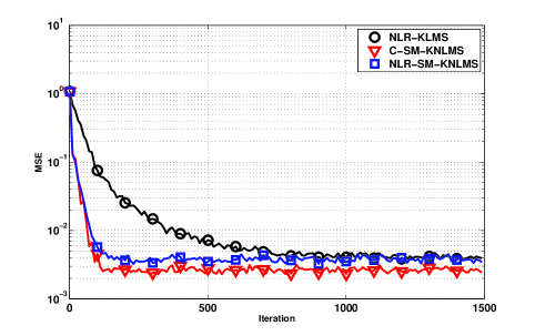
Refer to caption
Figure 1: Performance comparison of SM-KNLMS algorithms.

In the second example we evaluate the transient behavior of the NLR-SM-KNLMS. The input sequence x(i)𝑥𝑖x\left(i\right) is independent and identically Gaussian distributed with variance σx2=0.15subscriptsuperscript𝜎2𝑥0.15\sigma^{2}_{x}=0.15. We have also considered a fixed dictionary of length 161616. At each iteration, the dictionary elements were updated so that the oldest element added is replaced. To compute the learning curve, a total of 500500500 simulations were averaged, each one with 300030003000 iterations. The bandwidth of the Gaussian kernel was set to 0.0250.0250.025 for Fig. 2 and the threshold was set to γ=10σn𝛾10subscript𝜎𝑛\gamma=\sqrt{10}\sigma_{n} to obtain the results in Fig. 2.

Refer to caption
Figure 2: Transient behaviour of the SM-KNLMS algorithm. Bandwidth=0.025

In the third example, we assess the performance of the NLR-SM-KNLMS algorithm in a non-stationary environment. Particularly, we investigate the case when a sudden change occurs the system model, resulting in a different value of 𝜶𝒐subscript𝜶𝒐\boldsymbol{\alpha_{o}}. The two systems studied are given by

d1(i)=d(i1)1+d(i1)+x3(i1),subscript𝑑1𝑖𝑑𝑖11𝑑𝑖1superscript𝑥3𝑖1d_{1}\left(i\right)=\frac{d\left(i-1\right)}{1+d\left(i-1\right)}+x^{3}\left(i-1\right), (101)
d2(i)=x2(i).subscript𝑑2𝑖superscript𝑥2𝑖d_{2}\left(i\right)=x^{2}(i). (102)

In particular, a total of 800080008000 iterations were made, where the first 400040004000 iterations correspond to system d1subscript𝑑1d_{1}. Then, the system becomes unstable for 505050 iterations where d(i)=d(i1)+0.1𝑑𝑖𝑑𝑖10.1d(i)=d(i-1)+0.1. The remaining iterations correspond to system d2subscript𝑑2d_{2}. The output is corrupted by AWGN with standard deviation equal to σn=0.01subscript𝜎𝑛0.01\sigma_{n}=0.01. The input follows a Gaussian distribution with i.i.d samples and standard deviation given by σx=0.15subscript𝜎𝑥0.15\sigma_{x}=0.15.

Refer to caption
Figure 3: Performance of the NLR-SM-KNLMS algorithm in a non-stationary environment.

From Fig. 3 we note that NLR-SM-KNLMS is capable of tracking changes on the system and of converging to a new solution in few iterations. The solution obtained for system d2subscript𝑑2d_{2} achieves a lower MSE because the correlation between the mapped input and the desired signal is higher for this system. It is also important to mention that the simulation result matches the theoretical result.

In the fourth experiment we assess the performance of NLR-SM-KNLMS for correlated inputs. Let us consider two inputs, 𝐱c1subscript𝐱subscript𝑐1\mathbf{x}_{c_{1}} and 𝐱c2subscript𝐱subscript𝑐2\mathbf{x}_{c_{2}} each one with three different components i.e. 𝐱c(i)=[xc,1(i)xc,2(i)xc,3(i)]Tsubscript𝐱𝑐𝑖superscriptdelimited-[]subscript𝑥𝑐1𝑖subscript𝑥𝑐2𝑖subscript𝑥𝑐3𝑖𝑇\mathbf{x}_{c}\left(i\right)=\left[\begin{array}[]{ccc}x_{c,1}\left(i\right)&x_{c,2}\left(i\right)&x_{c,3}\left(i\right)\end{array}\right]^{T}. The correlation of the inputs satisfies

xc1,2(i)=0.5xc1,1(i)+δx(i)subscript𝑥subscript𝑐12𝑖0.5subscript𝑥subscript𝑐11𝑖subscript𝛿𝑥𝑖x_{c_{1},2}\left(i\right)=0.5x_{c_{1},1}\left(i\right)+\delta_{x}\left(i\right) (103)
xc2,2(i)=0.5xc2,1(i)+δx(i)subscript𝑥subscript𝑐22𝑖0.5subscript𝑥subscript𝑐21𝑖subscript𝛿𝑥𝑖x_{c_{2},2}\left(i\right)=0.5x_{c_{2},1}\left(i\right)+\delta_{x}\left(i\right) (104)
xc2,3(i)=0.2xc2,1(i)+0.4xc2,2(i)+δx(i)subscript𝑥subscript𝑐23𝑖0.2subscript𝑥subscript𝑐21𝑖0.4subscript𝑥subscript𝑐22𝑖subscript𝛿𝑥𝑖x_{c_{2},3}\left(i\right)=0.2x_{c_{2},1}\left(i\right)+0.4x_{c_{2},2}\left(i\right)+\delta_{x}\left(i\right) (105)

Both signals pass through a linear system with memory where the output is given by

y(i)=𝒓T𝐱c(i)0.3y(i1)+0.35y(i2)𝑦𝑖superscript𝒓𝑇subscript𝐱𝑐𝑖0.3𝑦𝑖10.35𝑦𝑖2y\left(i\right)=\boldsymbol{r}^{T}\mathbf{x}_{c}\left(i\right)-0.3y\left(i-1\right)+0.35y\left(i-2\right) (106)

with 𝒓=[10.50.3].𝒓delimited-[]10.50.3\boldsymbol{r}=\left[\begin{array}[]{ccc}1&0.5&0.3\end{array}\right]. A nonlinear function is then applied to y(i)𝑦𝑖y\left(i\right)

d(i){y(i)3(0.1+0.9y2(i))1/2y(i)0y2(i)[1e0.7y(i)]3y(i)<0𝑑𝑖cases𝑦𝑖3superscript0.10.9superscript𝑦2𝑖12𝑦𝑖0superscript𝑦2𝑖delimited-[]1superscript𝑒0.7𝑦𝑖3𝑦𝑖0d\left(i\right)\begin{cases}\frac{y\left(i\right)}{3\left(0.1+0.9y^{2}\left(i\right)\right)^{1/2}}&y\left(i\right)\geq 0\\ \frac{-y^{2}\left(i\right)\left[1-e^{0.7y\left(i\right)}\right]}{3}&y\left(i\right)<0\end{cases} (107)

The desired signal is corrupted by AWGN with σn=0.001subscript𝜎𝑛0.001\sigma_{n}=0.001. Fig. 4 illustrates the performance of NLR-KNLMS. The results show that the convergence speed for both inputs is similar. However, the correlation between the elements of the second input is stronger than that of the first input. This affects directly the performance of the NLR-SM-KNLMS as shown in Fig. 4, where we can see that the first input achieves a lower MSE than the second input.
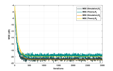
Refer to caption
Figure 4: Performance of the NLR-SM-KNLMS algorithm with correlated inputs.

In the last experiment of this section, we consider the identification of a Hammerstein system [84]. The input vector 𝐱(i)1×24𝐱𝑖superscript124{\mathbf{x}}(i)\in\mathbb{R}^{1\times 24} where each element has σx2=4×10⁴superscriptsubscript𝜎𝑥24superscript104\sigma_{x}^{2}=4\times 10^{-4} and the noise variance is σn=106subscript𝜎𝑛superscript106\sigma_{n}=10^{-6} . The kernel bandwidth was set to 0.0480.0480.048. The input goes through a nonlinear function to form the vector 𝐱~(i)~𝐱𝑖\tilde{\mathbf{x}}(i), where each element is given by

x~j(i)=xj3(i)subscript~𝑥𝑗𝑖superscriptsubscript𝑥𝑗3𝑖\tilde{x}_{j}\left(i\right)=x_{j}^{3}\left(i\right) (108)

The desired signal is obtained from a linear system expressed by

d(n)=𝐬T𝐱~(i)𝑑𝑛superscript𝐬𝑇~𝐱𝑖d\left(n\right)=\mathbf{s}^{T}\tilde{\mathbf{x}}\left(i\right) (109)

with s1=1subscript𝑠11s_{1}=1, s2=0.5subscript𝑠20.5s_{2}=0.5, s3=0.3subscript𝑠30.3s_{3}=0.3, s4=s5=s9=s13=s15=s19=s22=0.1subscript𝑠4subscript𝑠5subscript𝑠9subscript𝑠13subscript𝑠15subscript𝑠19subscript𝑠220.1s_{4}=s_{5}=s_{9}=s_{13}=s_{15}=s_{19}=s_{22}=0.1, s6=s7=0.2subscript𝑠6subscript𝑠70.2s_{6}=s_{7}=-0.2, s8=s10=s14=0.15subscript𝑠8subscript𝑠10subscript𝑠140.15s_{8}=s_{10}=s_{14}=-0.15, s18=0.15subscript𝑠180.15s_{18}=0.15, s9=,s11=0.12s_{9}=,s_{11}=0.12, s12=0.09subscript𝑠120.09s_{12}=-0.09, s16=0.05subscript𝑠160.05s_{16}=0.05, s17=0.05subscript𝑠170.05s_{17}=-0.05, s20=0.03subscript𝑠200.03s_{20}=0.03, s21=0.12subscript𝑠210.12s_{21}=-0.12, s23=0.02subscript𝑠230.02s_{23}=-0.02, s24=0.01subscript𝑠240.01s_{24}=-0.01.

Refer to caption
Figure 5: Performance of the NLR-SM-KNLMS algorithm for a Hammerstein system.

The results shown in Fig. 5 indicate that the learning speed of the proposed NLR-SM-KNLMS is lower than that for the identification of other nonlinear systems. This is because the Hammerstein system considered here has a larger number of parameters, which requires more iteration for the identification. The curves in Fig. 5 also show that the theoretical results agree well with those obtained by simulations.

VI-B Time series prediction

Let us now consider the performance of the proposed algorithms for a time series prediction task. We have used two different time series to perform the tests, the Mackey Glass time series [85] and a laser generated time series. First, we separate the data into two sets, one for training and the other for testing as suggested in [1]. The time-window was set to seven and the prediction step was set to one so that the last seven inputs of the time series were used to predict the value one step ahead. Additionally, both time series were corrupted by additive Gaussian noise with zero mean and standard deviation equal to 0.040.040.04. Using the Silverman rule and after several tests, the bandwidth of the kernel was optimized and the optimum value found was one.

First we evaluate the performance of the adaptive algorithms over the Mackey-Glass time series, which is generated by a nonlinear time difference equation that can be used to model nonlinear dynamics including chaos and represents a challenging time series for prediction tasks [85]. A total of 1500 sample inputs were used to generate the learning curve and the prediction was performed over 100 test samples. For the KLMS algorithm the step size was set to 0.050.050.05. The error bound for the C-SM-KNLMS algorithm was set to 5σ5𝜎\sqrt{5}\sigma. The final results of the algorithms tested are shown in Table II where the last 100 data points of each learning curve were averaged to obtain the MSE. The learning curves of the algorithms based on kernels is presented in Fig. 6. From the curves, we see that the proposed C-SM-KNLMS algorithm outperforms conventional algorithms in convergence speed.
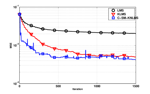
Refer to caption
Figure 6: Learning Curve of the Kernel Adaptive Algorithms for the Mackey-Glass Time Series prediction
TABLE II: Performance on Mackey-Glass time series prediction
Algorithm Test MSE Standard Deviation
LMS 0.023 +/-0.0002
NLMS 0.021 +/-0.0001
SM-NLMS 0.020 +/-0.0008
KLMS 0.007 +/-0.0003
C-SM-KNLMS 0.005 +/-0.0004

In the second example of this section, we consider the performance of the proposed algorithms over a laser generated time series, which is generated by chaotic intensity pulsations of a laser and also represents a challenging time series for prediction tasks [1]. In this case, 350035003500 sample inputs were used to generate the learning curves and the prediction was performed over 100 test samples. The setup used in the previous experiment was considered. Table III summarizes the MSE obtained for every algorithm tested. The learning curves are shown in Fig. 7.
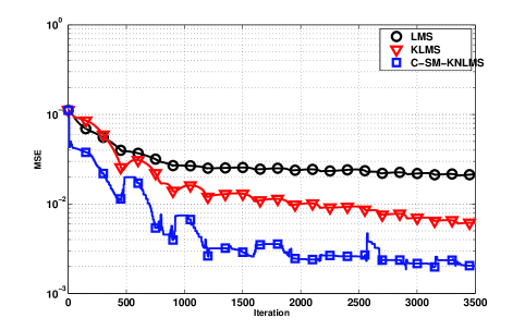
Refer to caption
Figure 7: Learning curves for the Laser Time Series prediction
TABLE III: Performance on laser generated time series prediction
Algorithm Test MSE Standard Deviation
LMS 0.021 +/-0.0003
NLMS 0.019 +/-0.001
SM-NLMS 0.024 +/-0.006
KLMS 0.009 +/-0.0006
C-SM-KNLMS 0.003 +/-0.0005

In the third experiment of this section we study the size of the dictionary generated by the conventional KLMS algorithm using different criteria to limit the size and by the proposed C-SM-KNLMS algorithm. The result is presented in Fig. 8. We notice that the proposed C-SM-KNLMS algorithm naturally limits the size of the dictionary. We also compare the performance of the C-SM-KNLMS with the performance obtained by the KLMS algorithm with different criteria. Fig. 9 summarizes the results, which shows that the proposed C-SM-KNLMS algorithm outperforms the existing algorithms by a significant margin.
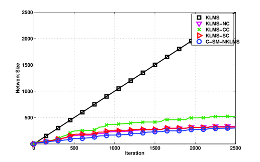
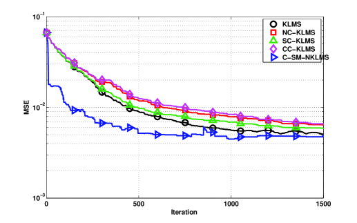
Refer to caption
Figure 8: Dictionary Size vs Iterations
Refer to caption
Figure 9: Performance comparison C-SM-KNLMS vs KLMS over time iterations.

In the last experiment, we have assessed the robustness of the proposed and existing algorithms for Gaussian noise with different values of standard deviation. Fig. 10 shows the results in terms of MSE performance against the noise standard deviation. The curves obtained in Fig. 10 indicate that the proposed C-SM-KNLMS algorithm outperforms the other algorithms for all the range of values of noise standard deviation considered. As expected the performance of all algorithms evaluated gradually degrade as the noise standard deviation increases.
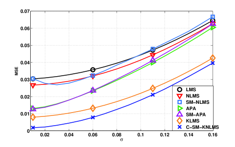
Refer to caption
Figure 10: Robustness performance of the studied algorithms versus standard deviation of noise.

VII Conclusions

In this paper, we have devised data-selective kernel-type algorithms, namely, the centroid-based and the nonlinear regression SM-KNLMS algorithms. The proposed SM-KNLMS algorithms have a faster convergence speed and a lower computational cost than the existing kernel-type algorithms in the same category. The proposed SM-KNLMS algorithms also have the advantage of naturally limiting the size of the dictionary created by kernel based algorithms and a satisfactory noise robustness. These features allow the proposed SM-KNLMS algorithms to solve nonlinear filtering and estimation problems with a large number of parameters without requiring a much longer training or computational cost. Simulations have shown that the proposed SM-KNLMS algorithms outperform previously reported techniques in examples of nonlinear system identification and prediction of a time series originating from a nonlinear difference equation.

Acknowledgment

The authors would like to thank the CNPq, and FAPERJ Brazilian agencies for funding.

References

  • [1] W. Liu, J. Príncipe, and S. Haykin, Kernel Adaptive Filtering: A Comprehensive Introduction., S. Haykin, Ed.   John Wiley & Sons, 2010.
  • [2] J. M. Gil-Cacho, M. Signoretto, T. van Waterschoot, M. Moonen, and S. Jensen, “Nonlinear acoustic echo cancellation based on a sliding-window leaky kernel affine projection algorithm.” IEEE Transactions on Audio, Speech and Language Processing, vol. 21, no. 9, pp. 1867 – 1878, April 2013.
  • [3] J. M. Gil-Cacho, T. van Waterschoot, M. Moonen, and S. Jensen, “Nonlinear acoustic echo cancellation based on a parallel-cascade kernel affine projection algorithm.” IEEE International Conference on Acoustics, Speech and Signal Processing, 2012.
  • [4] Y. Nakijama and M. Yukawa, “Nonlinear channel equalization by multi-kernel adaptive filter.” IEEE 13th International Workshop on Signal Processing Advances in Wireless Communications, 2012.
  • [5] C. Richard, J. Bermudez, and P. Honeine, “Online prediction of time series data with kernels.” IEEE Transactions on Signal Processing, vol. 57, no. 3, pp. 1058–1067, Feb. 2009.
  • [6] W. Liu, P. Pokharel, and J. Príncipe, “The kernel least-mean-squares algorithm.” IEEE Transactions on Signal Processing, vol. 56, no. 2, pp. 543–554, February 2008.
  • [7] P. Boboulis and S. Theodoridis, “Extension of wirtinger’s calculus to reproducing kernel hilbert spaces and the complex kernel LMS.” IEEE Transactions on Signal Processing, vol. 59, no. 3, pp. 964–978, March 2011.
  • [8] W. Liu and J. Príncipe, “Kernel affine projection algorithms.” EURASIP Journal on Advances in Signal Processing, vol. 2008, February 2008.
  • [9] K. Slavakis and S. Theodoridis, “Sliding window generalized kernel affine projection algorithm using projection mappings,” EURASIP Journal on Advances in Signal Processing, vol. 2008, no. 1, p. 735351, Apr 2008. [Online]. Available: https://doi.org/10.1155/2008/735351
  • [10] K. Slavakis, S. Theodoridis, and I. Yamada, “Online kernel-based classification using adaptive projection algorithms,” IEEE Transactions on Signal Processing, vol. 56, no. 7, pp. 2781–2796, July 2008.
  • [11] S. Theodoridis, K. Slavakis, and I. Yamada, “Adaptive learning in a world of projections,” IEEE Signal Processing Magazine, vol. 28, no. 1, pp. 97–123, Jan 2011.
  • [12] Y. Engel, S. Mannor, and R. Meir, “The kernel recursive least-squares algorithm.” IEEE Transactions on Signal Processing, vol. 52, no. 8, pp. 2275–2285, August 2004.
  • [13] W. Liu, Y. Wang, and J. Príncipe, “Extended kernel recursive least squares algorithm.” IEEE Transactions on Signal Processing, vol. 57, no. 10, pp. 3801–3814, May 2009.
  • [14] R. Pokharel, S. Seth, and J. Príncipe, “Mixture kernel least mean square.” The 2013 International Joint Conference on Neural Networks, 2013.
  • [15] M. Yukawa, “Multikernel adaptive filtering.” IEEE Transactions on Signal Processing, vol. 60, no. 9, pp. 4672 – 4682, August 2012.
  • [16] S. Van Vaerenbergh, J. Via, and I. Santamaria, “A sliding-window kernel RLS algorithm and its application to nonlinear channel identification.” IEEE International Conference on Acoustics, Speech and Signal Processing (ICASSP), 2006.
  • [17] S. Van Vaerenbergh, I. Santamaria, W. Liu, and J. Príncipe, “Fixed-budget kernel recursive least-squares.” IEEE International Conference on Acoustics, Speech and Signal Processing (ICASSP), 2010.
  • [18] F. Sheikholeslami, D. Berberidis, and G. B. Giannakis, “Kernel-based low-rank feature extraction on a budget for big data streams.” IEEE Global Conference on Signal and Information Processing (GlobalSIP), 2015.
  • [19] J. Platt, “A resource-allocating network for function interpolation.” Neural Computation, vol. 3, no. 3, pp. 213–225, 1991.
  • [20] W. Liu and J. Príncipe, “An information theoretic approach of designing sparse kernel adaptive filters.” IEEE Transactions on Neural Networks, vol. 20, no. 12, pp. 1950 – 1961, November 2009.
  • [21] A. Flores and R. C. de Lamare, “Set-membership kernel adaptive algorithms,” in Proceedings of IEEE International Conference on Acoustics, Speech and Signal Processing (ICASSP), March 2017, pp. 2676–2680.
  • [22] ——, “Set-membership adaptive kernel nlms algorithms: Design and analysis,” Signal Processing, 2018.
  • [23] E. Fogel and Y. F. Huang, “On the value of information in system identification-bounded noise case.” Automatica, vol. 18, pp. 229–238, March 1982.
  • [24] S. Gollamudi, S. Nagaraj, S. Kapoor, and Y. F. Huang, “Set-membership filtering and a set-membership normalized LMS algorithm with an adaptive step size.” IEEE Signal Processing Letters, vol. 5, no. 5, pp. 111–114, May 1998.
  • [25] S. Werner and P. Diniz, “Set-membership affine projection algorithm.” IEEE Signal Processing Letters, vol. 8, no. 8, pp. 231–235, August 2001.
  • [26] P. Diniz and S. Werner, “Set-membership binormalized data-reusing LMS algorithms.” IEEE Transactions on Signal Processing, vol. 51, no. 1, pp. 124–134, January 2003.
  • [27] R. C. de Lamare and P. Diniz, “Set-membership adaptive algorithms based on time-varying error bounds for CDMA interference suppression.” IEEE Transactions on Vehicular Technology, vol. 58, no. 2, pp. 644 – 654, February 2009.
  • [28] T. Wang, R. C. de Lamare, and P. D. Mitchell, “Low-complexity channel estimation for cooperative wireless sensor networks based on data selection,” in 2010 IEEE 71st Vehicular Technology Conference, May 2010, pp. 1–5.
  • [29] R. C. de Lamare and P. Diniz, “Blind adaptive interference suppression based on set-membership constrained constant-modulus algorithms with dynamic bounds.” IEEE Transactions on Signal Processing, vol. 61, no. 5, pp. 1288 – 1301, November 2012.
  • [30] T. Wang, R. C. de Lamare, and P. D. Mitchell, “Low-complexity set-membership channel estimation for cooperative wireless sensor networks,” IEEE Transactions on Vehicular Technology, vol. 60, no. 6, pp. 2594–2607, July 2011.
  • [31] K. Muller, S. Mika, G. Ratsch, K. Tsuda, and B. a. Scholkopf, “An introduction to kernel-based learning algorithms.” IEEE Transactions on Neural Networks, vol. 12, no. 2, pp. 181 – 201, March 2001.
  • [32] T. Wang, R. C. de Lamare, and A. Schmeink, “Alternating optimization algorithms for power adjustment and receive filter design in multihop wireless sensor networks,” IEEE Transactions on Vehicular Technology, vol. 64, no. 1, pp. 173–184, Jan 2015.
  • [33] R. C. de Lamare and R. Sampaio-Neto, “Adaptive reduced-rank mmse filtering with interpolated fir filters and adaptive interpolators,” IEEE Signal Processing Letters, vol. 12, no. 3, pp. 177–180, March 2005.
  • [34] ——, “Reduced-rank adaptive filtering based on joint iterative optimization of adaptive filters,” IEEE Signal Processing Letters, vol. 14, no. 12, pp. 980–983, Dec 2007.
  • [35] R. C. D. Lamare and R. Sampaio-Neto, “Minimum mean-squared error iterative successive parallel arbitrated decision feedback detectors for ds-cdma systems,” IEEE Transactions on Communications, vol. 56, no. 5, pp. 778–789, May 2008.
  • [36] R. C. de Lamare and R. Sampaio-Neto, “Adaptive reduced-rank processing based on joint and iterative interpolation, decimation, and filtering,” IEEE Transactions on Signal Processing, vol. 57, no. 7, pp. 2503–2514, July 2009.
  • [37] R. Fa, R. C. de Lamare, and L. Wang, “Reduced-rank stap schemes for airborne radar based on switched joint interpolation, decimation and filtering algorithm,” IEEE Transactions on Signal Processing, vol. 58, no. 8, pp. 4182–4194, Aug 2010.
  • [38] P. Li, R. C. de Lamare, and R. Fa, “Multiple feedback successive interference cancellation detection for multiuser mimo systems,” IEEE Transactions on Wireless Communications, vol. 10, no. 8, pp. 2434–2439, August 2011.
  • [39] T. Peng, R. C. de Lamare, and A. Schmeink, “Adaptive distributed space-time coding based on adjustable code matrices for cooperative mimo relaying systems,” IEEE Transactions on Communications, vol. 61, no. 7, pp. 2692–2703, July 2013.
  • [40] P. Clarke and R. C. de Lamare, “Transmit diversity and relay selection algorithms for multirelay cooperative mimo systems,” IEEE Transactions on Vehicular Technology, vol. 61, no. 3, pp. 1084–1098, March 2012.
  • [41] J. Gu, R. C. de Lamare, and M. Huemer, “Buffer-aided physical-layer network coding with optimal linear code designs for cooperative networks,” IEEE Transactions on Communications, vol. 66, no. 6, pp. 2560–2575, June 2018.
  • [42] Z. Yang, R. C. de Lamare, and X. Li, “l1subscript𝑙1l_{1}-regularized stap algorithms with a generalized sidelobe canceler architecture for airborne radar,” IEEE Transactions on Signal Processing, vol. 60, no. 2, pp. 674–686, Feb 2012.
  • [43] ——, “Sparsity-aware space-time adaptive processing algorithms with l1-norm regularisation for airborne radar,” IET Signal Processing, vol. 6, no. 5, pp. 413–423, July 2012.
  • [44] R. C. de Lamare, “Massive mimo systems: Signal processing challenges and future trends,” URSI Radio Science Bulletin, vol. 2013, no. 347, pp. 8–20, Dec 2013.
  • [45] R. C. de Lamare, R. Sampaio-Neto, and M. Haardt, “Blind adaptive constrained constant-modulus reduced-rank interference suppression algorithms based on interpolation and switched decimation,” IEEE Transactions on Signal Processing, vol. 59, no. 2, pp. 681–695, Feb 2011.
  • [46] R. C. de Lamare, “Adaptive and iterative multi-branch mmse decision feedback detection algorithms for multi-antenna systems,” IEEE Transactions on Wireless Communications, vol. 12, no. 10, pp. 5294–5308, October 2013.
  • [47] W. Zhang, H. Ren, C. Pan, M. Chen, R. C. de Lamare, B. Du, and J. Dai, “Large-scale antenna systems with ul/dl hardware mismatch: Achievable rates analysis and calibration,” IEEE Transactions on Communications, vol. 63, no. 4, pp. 1216–1229, April 2015.
  • [48] R. Fa and R. C. D. Lamare, “Reduced-rank stap algorithms using joint iterative optimization of filters,” IEEE Transactions on Aerospace and Electronic Systems, vol. 47, no. 3, pp. 1668–1684, July 2011.
  • [49] K. Zu, R. C. de Lamare, and M. Haardt, “Multi-branch tomlinson-harashima precoding design for mu-mimo systems: Theory and algorithms,” IEEE Transactions on Communications, vol. 62, no. 3, pp. 939–951, March 2014.
  • [50] L. Wang and R. C. D. Lamare, “Constrained adaptive filtering algorithms based on conjugate gradient techniques for beamforming,” IET Signal Processing, vol. 4, no. 6, pp. 686–697, Dec 2010.
  • [51] L. Landau, R. C. de Lamare, and M. Haardt, “Robust adaptive beamforming algorithms using the constrained constant modulus criterion,” IET Signal Processing, vol. 8, no. 5, pp. 447–457, July 2014.
  • [52] N. Song, R. C. de Lamare, M. Haardt, and M. Wolf, “Adaptive widely linear reduced-rank interference suppression based on the multistage wiener filter,” IEEE Transactions on Signal Processing, vol. 60, no. 8, pp. 4003–4016, Aug 2012.
  • [53] J. Liu and R. C. de Lamare, “Low-latency reweighted belief propagation decoding for ldpc codes,” IEEE Communications Letters, vol. 16, no. 10, pp. 1660–1663, October 2012.
  • [54] H. Ruan and R. C. de Lamare, “Robust adaptive beamforming using a low-complexity shrinkage-based mismatch estimation algorithm,” IEEE Signal Processing Letters, vol. 21, no. 1, pp. 60–64, Jan 2014.
  • [55] S. Xu, R. C. de Lamare, and H. V. Poor, “Distributed compressed estimation based on compressive sensing,” IEEE Signal Processing Letters, vol. 22, no. 9, pp. 1311–1315, Sept 2015.
  • [56] R. C. de Lamare and A. Alcaim, “Strategies to improve the performance of very low bit rate speech coders and application to a variable rate 1.2 kb/s codec,” IEE Proceedings - Vision, Image and Signal Processing, vol. 152, no. 1, pp. 74–86, Feb 2005.
  • [57] A. G. D. Uchoa, C. Healy, R. C. de Lamare, and R. D. Souza, “Design of ldpc codes based on progressive edge growth techniques for block fading channels,” IEEE Communications Letters, vol. 15, no. 11, pp. 1221–1223, November 2011.
  • [58] R. C. de Lamare and R. Sampaio-Neto, “Sparsity-aware adaptive algorithms based on alternating optimization and shrinkage,” IEEE Signal Processing Letters, vol. 21, no. 2, pp. 225–229, Feb 2014.
  • [59] N. Song, W. U. Alokozai, R. C. de Lamare, and M. Haardt, “Adaptive widely linear reduced-rank beamforming based on joint iterative optimization,” IEEE Signal Processing Letters, vol. 21, no. 3, pp. 265–269, March 2014.
  • [60] A. G. D. Uchoa, C. T. Healy, and R. C. de Lamare, “Iterative detection and decoding algorithms for mimo systems in block-fading channels using ldpc codes,” IEEE Transactions on Vehicular Technology, vol. 65, no. 4, pp. 2735–2741, April 2016.
  • [61] S. D. Somasundaram, N. H. Parsons, P. Li, and R. C. de Lamare, “Reduced-dimension robust capon beamforming using krylov-subspace techniques,” IEEE Transactions on Aerospace and Electronic Systems, vol. 51, no. 1, pp. 270–289, January 2015.
  • [62] P. Li and R. C. de Lamare, “Distributed iterative detection with reduced message passing for networked mimo cellular systems,” IEEE Transactions on Vehicular Technology, vol. 63, no. 6, pp. 2947–2954, July 2014.
  • [63] S. Li, R. C. de Lamare, and R. Fa, “Reduced-rank linear interference suppression for ds-uwb systems based on switched approximations of adaptive basis functions,” IEEE Transactions on Vehicular Technology, vol. 60, no. 2, pp. 485–497, Feb 2011.
  • [64] S. Xu, R. C. de Lamare, and H. V. Poor, “Adaptive link selection algorithms for distributed estimation,” EURASIP J. Adv. Signal Process., vol. 86, 2015.
  • [65] W. Zhang, R. C. de Lamare, C. Pan, M. Chen, J. Dai, B. Wu, and X. Bao, “Widely linear precoding for large-scale mimo with iqi: Algorithms and performance analysis,” IEEE Transactions on Wireless Communications, vol. 16, no. 5, pp. 3298–3312, May 2017.
  • [66] C. T. Healy and R. C. de Lamare, “Design of ldpc codes based on multipath emd strategies for progressive edge growth,” IEEE Transactions on Communications, vol. 64, no. 8, pp. 3208–3219, Aug 2016.
  • [67] Y. Cai, R. C. de Lamare, B. Champagne, B. Qin, and M. Zhao, “Adaptive reduced-rank receive processing based on minimum symbol-error-rate criterion for large-scale multiple-antenna systems,” IEEE Transactions on Communications, vol. 63, no. 11, pp. 4185–4201, Nov 2015.
  • [68] M. Yukawa, R. C. de Lamare, and R. Sampaio-Neto, “Efficient acoustic echo cancellation with reduced-rank adaptive filtering based on selective decimation and adaptive interpolation,” IEEE Transactions on Audio, Speech, and Language Processing, vol. 16, no. 4, pp. 696–710, May 2008.
  • [69] L. Wang, R. C. de Lamare, and M. Haardt, “Direction finding algorithms based on joint iterative subspace optimization,” IEEE Transactions on Aerospace and Electronic Systems, vol. 50, no. 4, pp. 2541–2553, October 2014.
  • [70] H. Ruan and R. C. de Lamare, “Robust adaptive beamforming based on low-rank and cross-correlation techniques,” IEEE Transactions on Signal Processing, vol. 64, no. 15, pp. 3919–3932, Aug 2016.
  • [71] T. G. Miller, S. Xu, R. C. de Lamare, and H. V. Poor, “Distributed spectrum estimation based on alternating mixed discrete-continuous adaptation,” IEEE Signal Processing Letters, vol. 23, no. 4, pp. 551–555, April 2016.
  • [72] L. Qiu, Y. Cai, R. C. de Lamare, and M. Zhao, “Reduced-rank doa estimation algorithms based on alternating low-rank decomposition,” IEEE Signal Processing Letters, vol. 23, no. 5, pp. 565–569, May 2016.
  • [73] S. F. B. Pinto and R. C. de Lamare, “Multi-step knowledge-aided iterative esprit: Design and analysis,” IEEE Transactions on Aerospace and Electronic Systems, pp. 1–1, 2018.
  • [74] R. Coelho, V. H. Nascimento, R. Queiroz, J. Romano, and C. Cavalcante, Eds., Signals and Images: Advances and Results in Speech, Estimation, Compression, Recognition, Filtering, and Processing.   CRC Press, 2015.
  • [75] B. Schölkopf, R. Herbrich, and J. Smola, “A generalized representer theorem.” 14th Annual Conference on Computational Learning Theory and 5th European Conference on Computational Learning Theory, pp. 416–426, 2001.
  • [76] J. Chen, W. Gao, C. Richard, and J. C. Bermudez, “Convergence analysis of kernel LMS algorithm with pre-tuned dictionary.” IEEE International Conference on Acoustics, Speech and Signal Processing (ICASSP), 2014.
  • [77] W. Parreira, J. C. Bermudez, C. Richard, and J. Tourneret, “Stochastic behavior analysis of the Gaussian kernel least-mean-square algorithm.” IEEE Transactions on Signal Processing, vol. 60, no. 5, pp. 2208 – 2222, January 2012.
  • [78] ——, “Steady-state behavior and design of the Gaussian KLMS algorithm.” European Signal Processing Conference (EUSIPCO), April 2011.
  • [79] J. Omura and T. Kailath, “Some useful probability distributions.” Stanford University, Tech. Rep. 7050-6, 1965.
  • [80] A. Sayed, Adaptive Filters.   John Wiley & Sons, 2008.
  • [81] R. Price, “A useful theorem for nonlinear devices having gaussian inputs,” IRE Transactions on Information Theory, vol. 4, no. 2, pp. 69–72, June 1958.
  • [82] K. S. Narendra and K. Parthasarathy, “Identification and control of synamical systems using neural networks,” IEEE Transactions on Neural Networks, vol. 1, no. 1, pp. 3–27, March 1990.
  • [83] D. P. Mandic, “A generalized normalized gradient descent algorithm,” IEEE Signal Processing Letters, vol. 2, pp. 115–118, February 2004.
  • [84] W. Greblicki and M. Pawlak, “Identification of discrete hammerstein systems using kernel regression estimates,” IEEE Transactions on Automatic Control, vol. 31, no. 1, pp. 74–77, January 1986.
  • [85] L. Glass and M. C. Mackey, “Pathological physiological conditions resulting from instabilities in physiological control systems,” Ann. NY. Acad. Sci, vol. 316, pp. 214–235, 1979.