A Structural-Factor Approach to Modeling High-Dimensional Time Series and Space-Time Data

Abstract

This paper considers a structural-factor approach to modeling high-dimensional time series and space-time data by decomposing individual series into trend, seasonal, and irregular components. For ease in analyzing many time series, we employ a time polynomial for the trend, a linear combination of trigonometric series for the seasonal component, and a new factor model for the irregular components. The new factor model simplifies the modeling process and achieves parsimony in parameterization. We propose a Bayesian Information Criterion (BIC) to consistently select the order of the polynomial trend and the number of trigonometric functions, and use a test statistic to determine the number of common factors. The convergence rates for the estimators of the trend and seasonal components and the limiting distribution of the test statistic are established under the setting that the number of time series tends to infinity with the sample size, but at a slower rate. We study the finite-sample performance of the proposed analysis via simulation, and analyze two real examples. The first example considers modeling weekly PM_2.5 data of 15 monitoring stations in the southern region of Taiwan and the second example consists of monthly value-weighted returns of 12 industrial portfolios.

Keywords: Bayesian information criterion, Canonical correlation analysis, Factor model, High-dimensional time series, Space-time data, PM_2.5, Seasonality, Trend.

1 Introduction

The availability of high-dimensional time series and space-time data under the current big-data environment creates new challenges in time series modeling, and analysis of such data has emerged as an important and active research area in many scientific fields, including engineering, environmental studies, and statistics. In theory, the vector autoregressive moving-average (VARMA) models can be used, but their applications often encounter the difficulties of over-parametrization and lack of identifiability, especially when the dimension is high. Over-parametrization is likely to occur when one uses unrestricted VARMA models, and it is well-known that exchangeable models exist in VARMA specification. See, for instance, Tiao and Tsay (1989), Lütkepohl (2006), Tsay (2014), and the references therein. Various methods have been developed to overcome the identifiability issues and to reduce the number of parameters of VARMA models. For example, Chapter 4 of Tsay (2014), and the references therein, discussed various canonical structures of a VARMA model. Davis et al. (2012) studied the vector autoregressive (VAR) model with sparse coefficient matrices based on partial spectral coherence. The Lasso regularization has also been applied to VAR models to reduce the number of parameters; see Shojaie and Michailidis (2010) and Song and Bickel (2011), among others. Guo et al. (2016) considered banded VAR models and estimated the coefficient matrices by a componentwise least squares method. For dimension reduction, popular methods include the canonical correlation analysis (CCA) of Box and Tiao (1977), the principle component analysis (PCA) of Stock and Watson (2002), and the scalar component analysis of Tiao and Tsay (1989). An alternative approach to analyzing high-dimensional time series is to employ factor models; see, for instance, Bai and Ng (2002), Stock and Watson (2005), Pan and Yao, (2008), Lam et al. (2011), Lam and Yao, (2012) and Chang et al., (2015). In fact, the idea of latent factors driving common behavior in multiple time series can be dated back, at least, to Nerlove (1964). Most of the factor models considered in the literature assume weak stationarity of the underlying time series and employ latent factors to describe the overall temporal dependence of the data.

Empirical time series often exhibit complex patterns, which may include trend and seasonal components. For example, the hourly measurements of fine particulate matter (PM_2.5) at different monitoring stations in a given region show not only an annual cycle but also certain diurnal pattern possibly caused by wind direction, wind speed, humidity, temperature, and human activities. The measurements may also exhibit some trending behavior due to increased urbanization, as some studies state that the urbanization level plays a positive role in promoting carbon emission, which is a major component of particulate matters. See, for example, Zhang et al. (2015). In the time series literature, structural models consisting of trend, seasonal, and irregular components have been proposed to analyze univariate series with complex patterns. See, for instance, Harvey (1989). As a matter of fact, a range of trend and periodic analyses for environmental and economic time series have appeared in the literature; see Wallis, (1978), Plosser, (1979), Barsky and Miron (1989), Harvey and Koopman (1993), Chang et al. (2009), De Livera et al. (2011), among others. However, none of those methods can be applied (or have been extended) to model jointly high-dimensional time series. Several methods have also been developed in the spatio-temporal literature to explore the spatial and temporal dependence of the data. See, for instance, Yu et al. (2008), Lee and Yu (2010), Lin and Lee (2010), Kelejian and Prucha (2010), Su (2012), and Gao et al. (2019), among others. However, most of the available methods require specification of a spatial weight matrix or an appropriate ordering of the locations. For a given application, the choices may not be obvious, and the resulting spatial autoregressive model may fail to accommodate adequately the dependent structure among different locations.

The goal of this paper is to combine the structural models with latent factors for analysis of high-dimensional time series and space-time data. By focusing on common factors for the irregular components rather than on the observed series directly, the proposed models can be more effective in identifying the number of common factors and can provide further insight in understanding the latent structure of the data. For instance, the identified common latent factors of the irregular components are free of the effects of trend or seasonality. Furthermore, the combined approach can leverage the advantages of structural specification and factor models. This is particularly relevant in analyzing high-dimensional and high-frequency data for which the common patterns can be complex and the observed data are typically non-Gaussian. Consider, for instance, the hourly measurements of PM_2.5 at a monitoring station. Such a series is often not normally distributed and exhibits annual, weekly, and diurnal patterns in addition to the local trending behavior. Figure 1(a) shows the time plot of hourly PM_2.5 measurements at a monitoring station in Taiwan from January 1, 2006 to December 31, 2015 for 87,600 observations (the data for February 29 were removed for simplicity). The traditional test statistics for skewness and excess kurtosis assume the values 99.5 and 56.9, respectively, with $p$-values close to zero. Figure 1(b) shows the sample autocorrelation functions (SACF) of the series. The upper plot contains 30,000 lags of SACF and it exhibits clearly an annual cycle with frequency $\omega=2\pi/8760$ = $7.17\times 10^{-4}$. The lower plot shows the first 200 lags of SACF and it also exhibits clearly an diurnal pattern with frequency $\omega_{1}=2\pi/24$ = 0.262. Thus, the cyclical patterns of the series are complex. Furthermore, the periodicity of 8760 is sufficiently large, making it hard to fit a seasonal ARMA model to the data. Finally, consider the situation in which many such PM_2.5 time series are available. It would not be simple to identify the overall latent factors among the series. This type of problem is not unique to environment studies. As a matter of fact, big data indexed by two or more indexes, such as the PM_2.5 in space and time, are routinely collected nowadays in many scientific fields. For example, in economics, monthly consumer price index (CPI) are collected for every member country of the European Union, and the state unemployment rates are compiled for the 50 states in the US. In finance, asset returns of many industrial portfolios or exchange-traded funds (ETF) are available daily. These data also exhibit complex cyclical (or seasonal) patterns. See Chang et al., (2009) and Chang and Pinegar, (1989) for details. In addition, researchers also found that a large number of economic variables can be modeled by a small number of factors, which provides a convenient way to study the aggregate implications of microeconomic behavior, as shown in Forni and Lippi, (1997). Examples such as these mentioned above motivate us to consider the proposed approach.

Figure 1: (a) Time plot of hourly PM_2.5 at a monitoring station in Taiwan from January 1, 2006 to December 31, 2015 for 87,600 observations; (b) Sample autocorrelation functions of the hourly time series of (a).

In applications, we often care about the general direction of the observed data over time. Therefore, for simplicity, we use a deterministic polynomial for the trend component and a linear combination of trigonometric functions for the seasonal component. This simplifying assumption is used mainly to overcome the difficulty in handling the high periodicity as that shown in the hourly PM_2.5 example. For the irregular components, we employ a new factor model to reduce the number of parameters and to describe the common stochastic characteristics of the data. The proposed factor model differs from the factor models commonly used in the literature, as we seek a nonsingular linear transformation that separates white noise series from the dynamically dependent ones. From a dimension reduction point of view, we treat the polynomial and trigonometric basis functions as the factors for the trend and seasonal components, respectively, and the latent stochastic factors for the irregular parts. The latent factors are linear combinations of the irregular components and are estimated by a canonical correlation analysis. The number of white noise series is determined by a test statistic. We propose a Bayesian Information Criterion (BIC) to consistently select the order of the polynomial trend and the number of the trigonometric functions. We also derive the convergence rates for the coefficient estimators of the trend and seasonal components and the limiting properties of the test statistic under the setting that the dimension of the time series tends to infinity with the sample size, but at a slower rate. Finally, we use simulation and real data examples to assess the performance of the proposed procedure.

The rest of the paper is organized as follows. We specify the proposed methodology in Section 2 with special attention being paid to the new factor model for the irregular components. The differences between the new model and the commonly used factor models in the literature are given. In Section 3, we study the theoretical properties of the proposed model. Section 4 reports the results of simulation studies and empirical applications of two examples. Section 5 provides concluding remarks. All technical proofs are relegated to an online supplement. We use the following notation, for a $p\times 1$ vector ${\mathbf{u}}=(u_{1},...,u_{p})^{\rm T},$ $||{\mathbf{u}}||_{2}=(\sum_{i=1}^{p}u_{i}^{2})^{1/2}$ is the Euclidean norm, and ${\mathbf{I}}_{p}$ denotes the $p\times p$ identity matrix. For a matrix ${\mathbf{H}}=(h_{ij})$, $|{\mathbf{H}}|_{\infty}=\max_{i,j}|h_{ij}|$, $\|{\mathbf{H}}\|_{2}=\sqrt{\lambda_{\max}({\mathbf{H}}^{\rm T}{\mathbf{H}})}$ is the operator norm, where $\lambda_{\max}(\cdot)$ denotes for the largest eigenvalue of a matrix, and $\|{\mathbf{H}}\|_{\min}$ is the square root of the minimum eigenvalue of ${\mathbf{H}}^{\rm T}{\mathbf{H}}$. The superscript ${\rm T}$ denotes the transpose of a vector or matrix. Finally, we use the notation $a\asymp b$ to denote $a=O(b)$ and $b=O(a)$.

2 Methodology

2.1 The Setting and Method

Let ${\mathbf{y}}_{t}=(y_{1t},...,y_{pt})^{{\rm T}}$ be a $p$-dimensional time series or an observation from $p$ spatial locations at time $t$. We assume that

$${\mathbf{y}}_{t}=\boldsymbol{\mu}_{t}+{\mathbf{s}}_{t}+\boldsymbol{\eta}_{t},$$ (2.1)

where $\boldsymbol{\mu}_{t}$, ${\mathbf{s}}_{t}$ and $\boldsymbol{\eta}_{t}$ denote, respectively, the trend, seasonal and irregular components with $\boldsymbol{\mu}_{t}=(\mu_{1t},...,\mu_{pt})^{{\rm T}}$, ${\mathbf{s}}_{t}=(s_{1t},...,s_{pt})^{{\rm T}}$, and $\boldsymbol{\eta}_{t}=(\eta_{1t},...,\eta_{pt})^{\rm T}$. For each $1\leq i\leq p$, we assume

$$\mu_{it}=\alpha_{i0}+\alpha_{i1}t+...+\alpha_{id_{0}}t^{d_{0}}\quad\text{and}\quad s_{it}=\sum_{j=1}^{k_{0}}[\beta_{ij}\cos(\rho_{j}t)+\gamma_{ij}\sin(\rho_{j}t)],$$ (2.2)

where $\rho_{j}=2\pi j/s$ with $s$ being a known periodicity, and $d_{0}$ and $k_{0}$ are nonnegative integers. The irregular component $\boldsymbol{\eta}_{t}$ is weakly stationary with $E(\boldsymbol{\eta}_{t})={\mathbf{0}}$ and can be written as

$$\boldsymbol{\eta}_{t}=\widetilde{\mathbf{L}}\left[\begin{array}[]{c}{\mathbf{f}}_{t}\\ \mbox{\boldmath$\varepsilon$}_{t}\end{array}\right]=\widetilde{\mathbf{L}}_{1}{\mathbf{f}}_{t}+\widetilde{\mathbf{L}}_{2}\mbox{\boldmath$\varepsilon$}_{t},$$ (2.3)

where $\widetilde{\mathbf{L}}=(\widetilde{\mathbf{L}}_{1},\widetilde{\mathbf{L}}_{2})$ is a $p\times p$ nonsingular (real-valued) matrix, ${\mathbf{f}}_{t}=(f_{1t},\ldots,f_{rt})^{\rm T}$ and $\mbox{\boldmath$\varepsilon$}_{t}=(\varepsilon_{1t},\ldots,\varepsilon_{vt})^{\rm T}$ with $r$ and $v$ being nonnegative integers such that $r+v=p$. Let ${\mathbf{V}}^{\rm T}=\widetilde{\mathbf{L}}^{-1}$ and ${\mathbf{V}}=({\mathbf{V}}_{1},{\mathbf{V}}_{2})$ with ${\mathbf{V}}_{1}\in R^{p\times r}$ and ${\mathbf{V}}_{2}\in R^{p\times v}$. Model (2.3) is a transformation model employed in Tiao and Tsay (1989). Specifically, there exists a nonsingular transformation matrix ${\mathbf{V}}$ such that ${\mathbf{V}}_{1}^{\rm T}\boldsymbol{\eta}_{t}={\mathbf{f}}_{t}$ and ${\mathbf{V}}_{2}^{\rm T}\boldsymbol{\eta}_{t}=\mbox{\boldmath$\varepsilon$}_{t}$ with dimensions $r$ and $v$, respectively.

In Equation (2.3), we assume that (a) $\mbox{\boldmath$\varepsilon$}_{t}$ is a $v$-dimensional scalar component process of order (0,0) if $v>0$, that is, Cov($\mbox{\boldmath$\varepsilon$}_{t},\boldsymbol{\eta}_{t-j}$) = ${\mathbf{0}}$ for $j>0$, and (b) no linear combination of ${\mathbf{f}}_{t}$ is a scalar component of order (0,0) if $r>0$. Assumption (b) is obvious; otherwise $v$ can be increased. For the formal definition of a general scalar component of order $(p_{1},q_{1})$ with $p_{1},q_{1}\geq 0$, readers are referred to Tiao and Tsay (1989). Assumption (a) is equivalent to $\mbox{\boldmath$\varepsilon$}_{t}$ being a white noise under the traditional factor models for which ${\mathbf{f}}_{t}$ and $\mbox{\boldmath$\varepsilon$}_{t}$ are assumed to be independent.

Any finite-order VARMA process $\boldsymbol{\eta}_{t}$ can always be written in Equation (2.3) via canonical correlation analysis (CCA) between two constructed vectors of $\boldsymbol{\eta}_{t}$ and its lagged variables. See Tiao and Tsay (1989). Also, readers are referred to Chapter 12 of Anderson (1958) for an introduction of CCA between two random vectors. Under Equation (2.3), the dynamic dependence of $\boldsymbol{\eta}_{t}$ is driven by ${\mathbf{f}}_{t}$ if $r>0$. In this sense, ${\mathbf{f}}_{t}$ indeed consists of the common factors of $\boldsymbol{\eta}_{t}$.

In contrast to Equation (2.3), the most commonly used factor model in the literature is

$$\boldsymbol{\eta}_{t}={\mathbf{A}}{\mathbf{x}}_{t}+\mbox{\boldmath$\varepsilon$}_{t},$$ (2.4)

where ${\mathbf{x}}_{t}\in R^{r}$ is a latent factor process, ${\mathbf{A}}\in R^{p\times r}$ is an unknown factor loading matrix, $\mbox{\boldmath$\varepsilon$}_{t}=(\varepsilon_{1t},...,\varepsilon_{pt})^{\rm T}$ is a serially uncorrelated process with mean $\bf 0$ and covariance matrix $\boldsymbol{\Sigma}_{\varepsilon}$, and ${\mathbf{x}}_{t}$ and $\mbox{\boldmath$\varepsilon$}_{t}$ are independent. See, for instance, Lam and Yao, (2012). A major difference between Equations (2.3) and (2.4) is that the right side of Equation (2.3) has $p$ random errors whereas that of Equation (2.4) has $r+p$ random errors. In this paper, we refer to the random errors, which consist of serially uncorrelated random variables with mean zero and finite covariance matrix, as innovations to a time series. Consequently, the sample covariance matrix of the innovation $\mbox{\boldmath$\varepsilon$}_{t}$ of Equation (2.4) is always singular if $r>0$. On the other hand, the sample covariance matrix of the innovation $\mbox{\boldmath$\varepsilon$}_{t}$ of Equation (2.3) is positive-definite provided that the sample size is sufficiently large.

Assume that $r>0$ in Equation (2.3). We further assume that ${\mathbf{f}}_{t}$ follows a vector autoregressive model, VAR($d$),

$${\mathbf{f}}_{t}=\sum_{i=1}^{d}\boldsymbol{\Phi}_{i}{\mathbf{f}}_{t-i}+{\mathbf{u}}_{t},$$ (2.5)

where ${\mathbf{u}}_{t}$ is a $r$-dimensional innovations with positive diagonal covariance matrix and independent of $\mbox{\boldmath$\varepsilon$}_{t}$. For large $r$, a sparse VAR model can be used. Under the VAR assumption in (2.5), the process $\boldsymbol{\eta}_{t}$ follows a VAR($d$) model with $\boldsymbol{\Phi}_{i}$ forming a non-zero block of the $i$th AR coefficient matrix. For a general $p$-dimensional zero-mean VAR($d$) model, the number of parameters is $dp^{2}+p(p+1)/2$, including those in the error covariance matrix. On the other hand, for the proposed model in Equations (2.3) and (2.5), the number of parameters is $p(p-1)/2+dr^{2}+p$, where $p(p-1)/2$ is the number of parameters in the transformation matrix. When $r$ is smaller than $p$, the proposed factor model becomes more parsimonious. For instance, consider the simple case of $p$ = 15, $r=10$, and $d$ = 1, the reduction in the number of parameters is $345-220$ = 125, which is not a small number. In general, the reduction in the number of parameters is $d(p^{2}-r^{2})$, which can be substantial if either $p$ or $d$ is large and $r$ is small.

In Equation (2.3), $({\mathbf{L}},{\mathbf{f}}_{t},\mbox{\boldmath$\varepsilon$}_{t})$ are all latent and any linear transformation of $\boldsymbol{\eta}_{t}$ will not alter the canonical correlation analysis between $\boldsymbol{\eta}_{t}$ and its lagged variables. Therefore, we consider the following transformed model

$$\boldsymbol{\Sigma}_{\eta}^{-1/2}\boldsymbol{\eta}_{t}={\mathbf{L}}\left[\begin{array}[]{c}{\mathbf{f}}_{t}\\ \mbox{\boldmath$\varepsilon$}_{t}\end{array}\right]={\mathbf{L}}_{1}{\mathbf{f}}_{t}+{\mathbf{L}}_{2}\mbox{\boldmath$\varepsilon$}_{t},$$ (2.6)

where $\boldsymbol{\Sigma}_{\eta}=\textnormal{Cov}(\boldsymbol{\eta}_{t})$ and ${\mathbf{L}}=({\mathbf{L}}_{1},{\mathbf{L}}_{2})=\boldsymbol{\Sigma}_{\eta}^{-1/2}\widetilde{\mathbf{L}}$ is a $p\times p$ orthonormal matrix. We will see later that this transformation can be done via canonical correlation analysis.

For Model (2.6), we refer to ${\mathbf{L}}_{1}$ the factor loading matrix of ${\mathbf{f}}_{t}$. The matrix ${\mathbf{L}}$ and the latent factor ${\mathbf{f}}_{t}$ are not uniquely determined in (2.6). For example, we can replace $({\mathbf{L}},{\mathbf{f}}_{t},\mbox{\boldmath$\varepsilon$}_{t})$ by $({\mathbf{L}}{\mathbf{H}},{\mathbf{H}}_{1}^{-1}{\mathbf{f}}_{t},{\mathbf{H}}_{2}^{-1}\mbox{\boldmath$\varepsilon$}_{t})$ for any invertible diagonal matrix ${\mathbf{H}}=\mbox{diag}({\mathbf{H}}_{1},{\mathbf{H}}_{2})$ and (2.6) still holds. Without loss of generality, we assume $\textnormal{Cov}(\boldsymbol{\xi}_{t})={\mathbf{I}}_{p}$, where $\boldsymbol{\xi}_{t}=({\mathbf{f}}_{t}^{{\rm T}},\mbox{\boldmath$\varepsilon$}_{t}^{{\rm T}})^{{\rm T}}$. Under this framework, it follows from (2.6) that ${\mathbf{L}}$ is an orthonormal matrix, i.e. ${\mathbf{L}}{\mathbf{L}}^{\rm T}={\mathbf{L}}^{\rm T}{\mathbf{L}}={\mathbf{I}}_{p}$. Note that, since canonical correlations may not be distinct, only $\mathcal{M}({\mathbf{L}}_{1})$ (and hence $\mathcal{M}({\mathbf{L}}_{2})$) can be uniquely determined, where $\mathcal{M}({\mathbf{L}}_{1})$ denotes the linear space spanned by the columns of the matrix ${\mathbf{L}}_{1}$ and is called the factor loading space.

Given the data $\{{\mathbf{y}}_{t}|t=1,...,T\}$, the goal here is to estimate the parameters $\boldsymbol{\alpha}_{i}=(\alpha_{i0},...,\alpha_{id_{0}})^{\rm T}$, $\boldsymbol{\beta}_{i}=(\beta_{i1},...,\beta_{ik_{0}})^{\rm T}$, $\boldsymbol{\gamma}_{i}=(\gamma_{i1},...,\gamma_{ik_{0}})^{\rm T}$ for $1\leq i\leq p$, ${\mathbf{L}}$ and the number of common factors $r$, and to recover the factor process ${\mathbf{f}}_{t}$, allowing the dimension $p$ to increase as the sample size $T$ increases, where $\boldsymbol{\alpha}_{i}$, $\boldsymbol{\beta}_{i}$ and $\boldsymbol{\gamma}_{i}$ are the coefficients defined in (2.2). In practice, $d_{0}$, $k_{0}$ and $r$ are also unknown and we propose methods to estimate them consistently in Section 2.2.

The proposed methodology is as follows. We first treat $d_{0}$ and $k_{0}$ as known integers and let $\boldsymbol{\theta}_{i}=(\boldsymbol{\alpha}_{i}^{\rm T},\boldsymbol{\beta}_{i}^{\rm T},\boldsymbol{\gamma}_{i}^{\rm T})^{\rm T}$, ${\mathbf{z}}_{i}=(y_{i1},...,y_{iT})^{\rm T}$ and ${\mathbf{e}}_{i}=(\eta_{i1},...,\eta_{iT})^{\rm T}$, where ${\mathbf{z}}_{i}$ and ${\mathbf{e}}_{i}$ denote, respectively, the $i$-th component of ${\mathbf{y}}_{t}$ and $\boldsymbol{\eta}_{t}$ over time. Define ${\mathbf{D}}=({\mathbf{d}}_{1},...,{\mathbf{d}}_{T})^{\rm T}$ with ${\mathbf{d}}_{t}=(1,t,...,t^{d_{0}},\cos(\rho_{1}t),...,\cos(\rho_{k_{0}}t),\sin(\rho_{1}t),...,\sin(\rho_{k_{0}}t))^{\rm T}$. Then, (2.1) can be expressed as

$${\mathbf{z}}_{i}={\mathbf{D}}\boldsymbol{\theta}_{i}+{\mathbf{e}}_{i},\quad i=1,...,p.$$ (2.7)

It follows from (2.7) that the ordinary least squares estimator (LSE) $\widehat{\boldsymbol{\theta}}_{i}$ for $\boldsymbol{\theta}_{i}$ satisfies

$$\widehat{\boldsymbol{\theta}}_{i}-\boldsymbol{\theta}_{i}=({\mathbf{D}}^{\rm T}{\mathbf{D}})^{-1}{\mathbf{D}}^{\rm T}{\mathbf{e}}_{i},\quad i=1,...,p,$$ (2.8)

and the associated residuals are $\widehat{\boldsymbol{\eta}}_{t}=(\widehat{\eta}_{1t},...,\widehat{\eta}_{pt})^{\rm T}$ with $\widehat{\eta}_{it}=y_{it}-{{\mathbf{d}}}_{t}^{\rm T}\widehat{\boldsymbol{\theta}}_{i}$. Furthermore, the resulting residual sum of squares is

$$\text{RSS}_{i}\equiv\text{RSS}_{i}(k_{0},d_{0})={\mathbf{z}}_{i}^{\rm T}\{{\mathbf{I}}_{T}-{\mathbf{D}}({\mathbf{D}}^{\rm T}{\mathbf{D}})^{-1}{\mathbf{D}}^{\rm T}\}{\mathbf{z}}_{i},\quad i=1,...,p,$$ (2.9)

where $\text{RSS}_{i}(k_{0},d_{0})$ is a function of $k_{0}$ and $d_{0}$, and we can similarly define $\text{RSS}_{i}(k,d)$ for any $1\leq k\leq s/2-1$ and $d\geq 0$. Note that $\widehat{\boldsymbol{\theta}}_{i}$’s are estimated equation-by-equation. Under the assumption that $\boldsymbol{\eta}_{t}$ is stationary, the estimators are equivalent to those of the generalized least squares method; see Section 2.5.1.1 of Tsay (2014) for a discussion on the estimation of VAR models.

Turn to the determination of the number of common factors $r$ and the estimation of ${\mathbf{L}}$. From Equation (2.6), we have

$${\mathbf{L}}^{-1}\boldsymbol{\Sigma}_{\eta}^{-1/2}\boldsymbol{\eta}_{t}={\mathbf{L}}^{\rm T}\boldsymbol{\Sigma}_{\eta}^{-1/2}\boldsymbol{\eta}_{t}=\left[\begin{array}[]{c}{\mathbf{f}}_{t}\\ \mbox{\boldmath$\varepsilon$}_{t}\end{array}\right].$$ (2.10)

Thus, there are $v$ linear combinations of $\boldsymbol{\eta}_{t}$ that are scalar components of order (0,0) and we can apply the approach of Tiao and Tsay (1989) to specify $v$ and, hence, $r=p-v$.

Let $\boldsymbol{\eta}_{t,m}=(\boldsymbol{\eta}_{t-1}^{\rm T},\ldots,\boldsymbol{\eta}_{t-m}^{\rm T})^{\rm T}$ be the vector of past $m$ lagged values of $\boldsymbol{\eta}_{t}$, where $m$ is a sufficiently large positive integer. Since $\mbox{\boldmath$\varepsilon$}_{t}$ are scalar components of order (0,0), we have Cov($\mbox{\boldmath$\varepsilon$}_{t}$,$\boldsymbol{\eta}_{t,m}$) = ${\mathbf{0}}$. Consequently, there are $v$ zero canonical correlations between $\boldsymbol{\eta}_{t}$ and $\boldsymbol{\eta}_{t,m}$. Let $\boldsymbol{\Sigma}_{\eta\eta_{m}}=\textnormal{Cov}(\boldsymbol{\eta}_{t},\boldsymbol{\eta}_{t,m})$ and $\boldsymbol{\Sigma}_{\eta_{m}}=\textnormal{Cov}(\boldsymbol{\eta}_{t,m})$. The canonical correlation analysis between $\boldsymbol{\eta}_{t}$ and $\boldsymbol{\eta}_{t,m}$ is the eigenvalue and eigenvector analysis of the matrix

$${\mathbf{M}}=\boldsymbol{\Sigma}_{\eta}^{-1/2}\boldsymbol{\Sigma}_{\eta\eta_{m}}\boldsymbol{\Sigma}_{\eta_{m}}^{-1}\boldsymbol{\Sigma}_{\eta_{m}\eta}\boldsymbol{\Sigma}_{\eta}^{-1/2}.$$ (2.11)

It is easy to see that rank(${\mathbf{M}}$) = $r$. Furthermore, let $\boldsymbol{\xi}_{t,m}=(\boldsymbol{\xi}_{t-1}^{\rm T},\ldots,\boldsymbol{\xi}_{t-m}^{\rm T})^{\rm T}$, where again $\boldsymbol{\xi}_{t}=({\mathbf{f}}_{t}^{{\rm T}},\mbox{\boldmath$\varepsilon$}_{t}^{{\rm T}})^{{\rm T}}$, and define $\boldsymbol{\Sigma}_{\xi}$, $\boldsymbol{\Sigma}_{\xi\xi_{m}}$ and $\boldsymbol{\Sigma}_{\xi_{m}}$ as the covariance matrices of the given random vectors. It is easy to verify that

$${\mathbf{M}}={\mathbf{L}}\boldsymbol{\Sigma}_{\xi{\xi_{m}}}\boldsymbol{\Sigma}_{\xi_{m}}^{-1}\boldsymbol{\Sigma}_{{\xi_{m}}\xi}{\mathbf{L}}^{\rm T}={\mathbf{L}}_{1}\boldsymbol{\Sigma}_{f{\xi_{m}}}\boldsymbol{\Sigma}_{\xi_{m}}^{-1}\boldsymbol{\Sigma}_{{\xi_{m}}f}{\mathbf{L}}_{1}^{\rm T}.$$

Let $\lambda_{1}^{2}\geq\lambda_{2}^{2}\geq\cdots\geq\lambda_{p}^{2}$ be the ordered eigenvalues of ${\mathbf{M}}$ and let $[{\mathbf{a}}_{1},{\mathbf{a}}_{2},\ldots,{\mathbf{a}}_{p}]$ be the corresponding eigenvectors. Then, $\lambda_{r}\neq 0$, but $\lambda_{j}=0$ for $j>r$, and we may take ${\mathbf{L}}=[{\mathbf{a}}_{1},\cdots,{\mathbf{a}}_{p}]$, which is an orthonormal matrix. Making use of the properties of canonical correlation analysis, we have

$${\mathbf{L}}^{{\rm T}}\boldsymbol{\Sigma}_{\eta}^{-1/2}\boldsymbol{\eta}_{t}=\boldsymbol{\xi}_{t},$$

and Cov($\boldsymbol{\xi}_{t}$) = ${\mathbf{I}}_{p}$. Thus, $\boldsymbol{\xi}_{t}={\mathbf{L}}^{\rm T}\boldsymbol{\Sigma}_{\eta}^{-1/2}\boldsymbol{\eta}_{t}$, ${\mathbf{L}}_{1}=[{\mathbf{a}}_{1},\ldots,{\mathbf{a}}_{r}]$ is the loading matrix of the common factors ${\mathbf{f}}_{t}$, and ${\mathbf{L}}_{2}=[{\mathbf{a}}_{r+1},\ldots,{\mathbf{a}}_{p}]$. This shows that the model in (2.3) always exists for a VARMA process $\boldsymbol{\eta}_{t}$. Furthermore, if the $r$ non-zero eigenvalues of ${\mathbf{M}}$ are distinct, ${\mathbf{L}}_{1}$ is uniquely defined if we ignore the trivial replacement of ${\mathbf{a}}_{j}$ by $-{\mathbf{a}}_{j}$.

Let

$$\widehat{\boldsymbol{\Sigma}}_{\eta}=\frac{1}{T}\sum_{t=1}^{T}(\widehat{\boldsymbol{\eta}}_{t}-\bar{\boldsymbol{\eta}})(\widehat{\boldsymbol{\eta}}_{t}-\bar{\boldsymbol{\eta}})^{\rm T},$$ (2.12)

where $\bar{\boldsymbol{\eta}}=\sum_{t=1}^{T}\widehat{\boldsymbol{\eta}}_{t}/T$. The sample estimators $\widehat{\boldsymbol{\Sigma}}_{\eta_{m}}$, $\widehat{\boldsymbol{\Sigma}}_{\eta\eta_{m}}$ are defined in a similar way and the index exceeds $1$ or $T$ are set to be $0$. This leads to the following natural estimator for ${\mathbf{M}}$,

$$\widehat{{\mathbf{M}}}=\widehat{\boldsymbol{\Sigma}}_{\eta}^{-1/2}\widehat{\boldsymbol{\Sigma}}_{\eta\eta_{m}}\widehat{\boldsymbol{\Sigma}}_{\eta_{m}}^{-1}\widehat{\boldsymbol{\Sigma}}_{\eta_{m}\eta}\widehat{\boldsymbol{\Sigma}}_{\eta}^{-1/2}.$$ (2.13)

The above discussion also gives rise to an estimator of ${\mathbf{L}}$ as $\widehat{{\mathbf{L}}}=(\widehat{{\mathbf{a}}}_{1},...,\widehat{{\mathbf{a}}}_{r},\widehat{\mathbf{a}}_{r+1},...,\widehat{\mathbf{a}}_{p})$, where $\widehat{{\mathbf{a}}}_{1},...,\widehat{{\mathbf{a}}}_{r}$ are the orthonormal eigenvectors of $\widehat{{\mathbf{M}}}$ corresponding to the $r$ largest eigenvalues $\widehat{\lambda}_{1}^{2}\geq\cdots\geq\widehat{\lambda}_{r}^{2}$, and $\widehat{{\mathbf{a}}}_{r+1},\ldots,\widehat{{\mathbf{a}}}_{p}$ are the orthonormal eigenvectors of $\widehat{{\mathbf{M}}}$ corresponding to the $p-r$ smallest eigenvalues $\widehat{\lambda}_{r+1}^{2}\geq\cdots\geq\widehat{\lambda}_{p}^{2}$. Since $\widehat{{\mathbf{L}}}$ is an orthonormal matrix, i.e. $\widehat{{\mathbf{L}}}^{{\rm T}}\widehat{{\mathbf{L}}}={\mathbf{I}}_{p}$, we may extract the factor process by $\widehat{{\mathbf{f}}}_{t}=\widehat{{\mathbf{L}}}_{1}^{\rm T}\widehat{\boldsymbol{\Sigma}}_{\eta}^{-1/2}\widehat{\boldsymbol{\eta}}_{t}$.

2.2 Selections of $d_{0}$, $k_{0}$, and $r$

The estimation of $\boldsymbol{\theta}_{i}$ in (2.8) assumes $d_{0}$ and $k_{0}$ are known, but these integers must be estimated in practice. We propose to determine $k_{0}$ and $d_{0}$ based on the following marginal Bayesian information criterion,

$$\text{BIC}_{i}(k,d)=\log[\text{RSS}_{i}(k,d)/T]+\frac{d+k}{T}C_{T}\log(p\vee T),\quad i=1,...,p,$$ (2.14)

where $\text{RSS}_{i}(k,d)$ is similarly defined as (2.9) for some $k$ and $d$, $p\vee T=\max(p,T)$, and $C_{T}>0$ is some constant which diverges together with $T$; see Assumption 3 in Section 3. We often take $C_{T}$ to be $\log\{\log(T)\}$. Let $\bar{k}$ and $\bar{d}$ be two pre-specified integers and

$$(\widehat{k}_{i},\widehat{d}_{i})=\arg\min_{1\leq k\leq\bar{k},1\leq d\leq\bar{d}}\text{BIC}_{i}(k,d),\quad i=1,...,p.$$ (2.15)

We take $\widehat{k}=\max_{1\leq i\leq p}\widehat{k}_{i}$ and $\widehat{d}=\max_{1\leq i\leq p}\widehat{d}_{i}$ as the estimators of $k_{0}$ and $d_{0}$, respectively. Theorem 2 in Section 3 shows that under some assumptions, $P(\widehat{k}=k_{0},\widehat{d}=d_{0})\rightarrow 1$ as $T$ and $p\rightarrow\infty$.

Remark 1.

In practice, $d_{0}=1$ or $2$ is often sufficient in characterizing the trend of many time series and space-time data. Therefore, we may fix $d_{0}$ and use the following estimator for $k_{0}$,

$$\widehat{k}=\max_{1\leq i\leq p}\{\arg\min_{1\leq k\leq\bar{k}}\text{BIC}_{i}(k,d_{0})\}.$$ (2.16)

Our numerical study shows that the procedure is insensitive to the choice of $\bar{k}$ provided $\bar{k}\geq k_{0}$ and $\bar{k}\leq s/2-1$, which is the maximum possible value to avoid any singularity, or choose $\bar{k}$ by checking the curvature of $\text{BIC}_{i}(k)$ directly.

Turn to the estimation of $r$, which plays an important role in the proposed statistical inference. In practice, we may estimate the number of zero canonical correlations $v$ (and hence $r$) by testing the null hypothesis $H_{0}:\lambda_{p-v+1}^{2}=\cdots=\lambda_{p}^{2}=0$ and $\lambda_{p-v}^{2}\neq 0$ versus the alternative hypothesis $H_{a}:\lambda_{p-v}^{2}=0$, where $\lambda_{i}^{2}$ are the ordered eigenvalues of ${\mathbf{M}}$. A test statistic available for testing the hypothesis is

$$S_{T}(v)=-(T-m+1)\sum_{i=1}^{v}\log(1-\widehat{\lambda}_{p-i+1}^{2}).$$ (2.17)

See Tiao and Tsay (1989). Under the null hypothesis and some regularity conditions, $S_{T}(v)$ is distributed as $\chi^{2}_{v[(m-1)p+v]}$. Since we allow for the dimension $p$ to increase with the sample $T$, we modify the test statistic accordingly by making use of the central limit theorem and properties of $\chi^{2}$ random variables. Specifically, we employ a standardized version of the test statistic:

$$C_{T}(v)=\frac{S_{T}(v)-v[(m-1)p+v]}{\sqrt{2v[(m-1)p+v]}}.$$ (2.18)

Then, under the null hypothesis and some regularity conditions, $C_{T}(v)$ converges in distribution to N(0,1) as $p\rightarrow\infty$. Note that the test statistic in Equation (2.17) is for testing the number of scalar components of order (0,0) so that there is no need to consider the normalization of eigenvalues. Details are given in Tiao and Tsay (1989).

Using the test statistics in (2.17) or (2.18), one can perform the hypothesis testing sequentially starting with $v=1$ and until the null hypothesis is rejected. The resulting number of zero eigenvalues $\widehat{v}$ is an estimate of $v$, and we have $\widehat{r}=p-\widehat{v}$.

3 Theoretical Properties

We present some asymptotic theory for the estimation methods described in Section 2 when $T$, $p\rightarrow\infty$. We assume $\{({\mathbf{y}}_{t},{\mathbf{f}}_{t})\}$ is $\alpha$-mixing with the mixing coefficients defined by

$$\alpha_{p}(k)=\sup_{i}\sup_{A\in\mathcal{F}_{-\infty}^{i},B\in\mathcal{F}_{i+k}^{\infty}}|P(A\cap B)-P(A)P(B)|,$$ (3.1)

where $\mathcal{F}_{i}^{j}$ is the $\sigma$-field generated by $\{({\mathbf{y}}_{t},{\mathbf{f}}_{t}):i\leq t\leq j\}$.

Assumption 1.

The process $\{({\mathbf{y}}_{t},{\mathbf{f}}_{t})\}$ is $\alpha$-mixing with the mixing coefficients satisfying the condition $\sum_{k=1}^{\infty}\alpha_{p}(k)^{1-2/\gamma}<\infty$ for some $\gamma>2$, where $\alpha_{p}(k)$ is defined in (3.1).

Assumption 2.

For any $i=1,...,p$, $E|\eta_{it}|^{2\gamma}\leq C_{1}$, where $C_{1}>0$ is a constant, $\gamma$ is given in Assumption 1.

Assumption 1 is standard for dependent random sequences. See Gao et al. (2018) for a theoretical justification for VAR models. The condition $E|\eta_{it}|^{2\gamma}\leq C_{1}$ in Assumption 2 can be guaranteed by some suitable conditions on $\xi_{it}$ and each row of $\widetilde{\mathbf{L}}$ defined in Equation (2.3). For example, it holds if $\max_{i,t}E|\xi_{it}|^{2\gamma}<\infty$ and $\max_{i}\sum_{j=1}^{p}|\widetilde{\mathbf{L}}_{ij}|<\infty$, where $\widetilde{\mathbf{L}}_{ij}$ is the $(i,j)$-th element of $\widetilde{\mathbf{L}}$. The following theorem establishes the convergence rates of the coefficient estimates for the trend and seasonal parts component-wisely.

Theorem 1.

If Assumptions 1-2 hold and $k_{0}$ and $d_{0}$ are known, as $T,p\rightarrow\infty$, we have

$$|\widehat{\alpha}_{ij}-\alpha_{ij}|=O_{p}(T^{-(2j+1)/2}),\,\,|\widehat{\beta}_{il}-\beta_{il}|=O_{p}(T^{-1/2})\,\,\text{and}\,\,|\widehat{\gamma}_{il}-\gamma_{il}|=O_{p}(T^{-1/2}),$$

for $1\leq i\leq p$, $0\leq j\leq d_{0}$ and $1\leq l\leq k_{0}$.

Theorem 1 implies that the convergence rates do not depend on the dimension $p$, which is reasonable since the dimension of each $\boldsymbol{\theta}_{i}$ is finite. Thus, they are as optimal as the regression estimators with the dimension fixed. To show the consistency of the selected $\widehat{k}$ and $\widehat{d}$ by BIC, we need to impose a condition on the magnitude of the coefficients of the largest orders of the time trend and seasonal components.

Assumption 3.

For each $i=1,...,p$, $\alpha_{id_{0}}^{2}>>C_{T}(d_{0}+k_{0})/T\log(p\vee T)$ and $\beta_{ik_{0}}^{2}+\gamma_{ik_{0}}^{2}>>C_{T}(d_{0}+k_{0})/T\log(p\vee T)$, where $C_{T}\rightarrow\infty$ as $T\rightarrow\infty$.

Assumption 3 ensures that the orders of the polynomial trend ($d_{0}$) and the number of the trigonometric series ($k_{0}$) are asymptotically identifiable in the sense that their coefficients can be detected as non-zero ones as $\{T^{-1}\log(p\vee T)\}^{1/2}$ is the minimum order of a non-zero coefficient to be identifiable; see, for instance, Luo and Chen (2013).

We now state the consistency of the selectors $\widehat{k}$ and $\widehat{d}$ defined in (2.15).

Theorem 2.

If Assumptions 1-3 hold, then $P(\widehat{k}=k_{0},\widehat{d}=d_{0})\rightarrow 1$ as $T,p\rightarrow\infty$.

Theorem 2 implies that we can consistently estimate $d_{0}$ and $k_{0}$ under some regularity conditions as the dimension $p$ and the sample size $T$ go to infinity. Therefore, we can replace $d_{0}$ and $k_{0}$ by $\widehat{d}$ and $\widehat{k}$, respectively, in the estimators $\boldsymbol{\theta}_{i}$ in Section 2. To establish the results for estimating factor loadings, we introduce more assumptions.

Assumption 4.

There exist positive constants $C_{2}$, $C_{3}$, $C_{4}$, $\kappa_{1}$ and $\kappa_{2}$ such that $\|\boldsymbol{\Sigma}_{f{\xi_{m}}}\|_{2}\leq C_{2}$ and $C_{3}\leq\|\boldsymbol{\Sigma}_{\xi_{m}}\|_{\min}\leq\|\boldsymbol{\Sigma}_{\xi_{m}}\|_{2}\leq C_{4}$, and $\kappa_{1}\leq\lambda_{\min}(\widetilde{\mathbf{L}}\widetilde{\mathbf{L}}^{\rm T})\leq\lambda_{\max}(\widetilde{\mathbf{L}}\widetilde{\mathbf{L}}^{{\rm T}})\leq\kappa_{2}$, where $\kappa_{1}$ and $\kappa_{2}$ may diverge in relation to the dimension $p$.

Assumption 5.

The matrix ${\mathbf{M}}$ admits $r$ distinct positive eigenvalues $\lambda_{1}^{2}>\cdots>\lambda_{r}^{2}>0$.

The boundedness condition of the eigenvalues of $\boldsymbol{\Sigma}_{f\xi_{m}}$ and $\boldsymbol{\Sigma}_{\xi_{m}}$ in Assumption 4 is natural since we have standardized $\boldsymbol{\xi}_{t}$ to $\textnormal{Cov}(\boldsymbol{\xi}_{t})={\mathbf{I}}_{p}$, and is related to the dimension $p$ since the columns of ${\mathbf{L}}_{1}$ are standardized. $\kappa_{1}$ and $\kappa_{2}$ of Assumption 4 control the strength of the transformation matrix $\widetilde{\mathbf{L}}$. Assumption 5 implies that ${\mathbf{L}}_{1}$ defined in Section 2.2 is unique. This simplifies the presentation significantly, as Theorem 3 below can present the convergence rates of the estimator for ${\mathbf{L}}_{1}$ directly. Without Assumption 5, the same convergence rates can be obtained for the estimation of the linear space $\mathcal{M}(\widehat{{\mathbf{L}}}_{1})$; see (3.3) in Theorem 4 below.

Theorem 3.

If Assumptions 1-5 hold and suppose that $r$ is known and fixed, then

$$\|\widehat{{\bf L}}_{i}-{\bf L}_{i}\|_{2}=~{}\left\{\begin{array}[]{ll}O_{p}(T^{-1/2}),&{\rm if\;\;}p\text{\rm\;\; is fixed};\\[4.30554pt] O_{p}(\kappa_{1}^{-2}\kappa_{2}pT^{-1/2}),&{\rm if\;}p=o\{\min(T^{1/2},\kappa_{2}^{-1}\kappa_{1}^{2}T^{1/2})\};i=1,2.\end{array}\right.$$

Furthermore,

$$p^{-1/2}\|\widehat{{\bf L}}_{1}\widehat{{\bf f}}_{t}-{\bf L}_{1}{\bf f}_{t}\|_{2}$$

$$=\left\{\begin{array}[]{ll}O_{p}(T^{-1/2}),&{\rm if}\;p\;\text{\rm is fixed};\\[4.30554pt] O_{p}(\|\widehat{\mathbf{L}}_{1}-{\mathbf{L}}_{1}\|_{2}+\kappa_{1}^{-3/2}p^{3/2}T^{-1/2}+\kappa_{1}^{-1/2}p^{1/2}T^{-1/2}),&{\rm if}\;p=o\{\min(T^{1/2},\kappa_{2}^{-1}\kappa_{1}^{2}T^{1/2})\}.\end{array}\right.$$

From Theorem 3 and, as expected, the convergence rates are all standard at $\sqrt{T}$, which is commonly seen in the traditional statistical theory. When $p$ is diverging, the upper bounds in Theorem 3 are all $pT^{-1/2}$ if we assume $\kappa_{1}$ and $\kappa_{2}$ are finite, implying that the condition $p=o(T^{1/2})$ is needed to guarantee the consistency. On the other hand, if $\kappa_{1}\asymp\kappa_{2}\asymp T^{\iota}$ for some $0<\iota<1$, we have $\|\widehat{{\bf L}}_{i}-{\bf L}_{i}\|_{2}=O_{p}(p^{1-\iota}T^{-1/2})$ and $p^{-1/2}\|\widehat{{\bf L}}_{1}\widehat{{\bf f}}_{t}-{\bf L}_{1}{\bf f}_{t}\|_{2}=O_{p}(p^{3(1-\iota)/2}T^{-1/2})$. Therefore, we need $p=o(T^{1/(3(1-\iota))})$ in this case. For example, if $\iota=1/4$, then the condition becomes $p=o(T^{4/9})$ to guarantee the consistency.

In general, the choice of ${\mathbf{L}}_{1}$ in Model (2.4) is not unique so we consider the error in estimating $\mathcal{M}({\mathbf{L}}_{1})$ instead of a particular ${\mathbf{L}}_{1}$, because $\mathcal{M}({\mathbf{L}}_{1})$ is uniquely defined by (2.4) and it does not vary with different choices of ${\mathbf{L}}_{1}$. To this end, we adopt the discrepancy measure used by Pan and Yao, (2008): for two $p\times r$ half orthogonal matrices ${\bf H}_{1}$ and ${\bf H}_{2}$ satisfying the condition ${\bf H}_{1}^{\rm T}{\bf H}_{1}={\bf H}_{2}^{\rm T}{\bf H}_{2}={\mathbf{I}}_{r}$, the difference between the two linear spaces $\mathcal{M}({\bf H}_{1})$ and $\mathcal{M}({\bf H}_{2})$ is measured by

$$D(\mathcal{M}({\bf H}_{1}),\mathcal{M}({\bf H}_{2}))=\sqrt{1-\frac{1}{r}\textrm{tr}({\bf H}_{1}{\bf H}_{1}^{\rm T}{\bf H}_{2}{\bf H}_{2}^{\rm T})}.$$ (3.2)

Note that $D(\mathcal{M}({\bf H}_{1}),\mathcal{M}({\bf H}_{2}))$ always assumes values between 0 and 1. It is equal to $0$ if and only if $\mathcal{M}({\bf H}_{1})=\mathcal{M}({\bf H}_{2})$, and to $1$ if and only if $\mathcal{M}({\bf H}_{1})\perp\mathcal{M}({\bf H}_{2})$. The following theorem establishes the convergence of $D(\mathcal{M}(\widehat{\bf L}_{1}),\mathcal{M}({\bf L}_{1}))$ when ${\mathbf{L}}_{1}$ is not uniquely defined.

Theorem 4.

Suppose Assumptions 1-4 hold. Assume that $r$ is known and fixed, then for $i=1,2$,

$$D(\mathcal{M}(\widehat{\bf L}_{i}),\mathcal{M}({\bf L}_{i}))=~{}\left\{\begin{array}[]{ll}O_{p}(T^{-1/2}),&{\rm if\;\;}p\text{\rm\;\; is fixed};\\[4.30554pt] O_{p}(\kappa_{1}^{-2}\kappa_{2}pT^{-1/2}),&{\rm if\;}p=o\{\min(T^{1/2},\kappa_{2}^{-1}\kappa_{1}^{2}T^{1/2})\}.\end{array}\right.$$ (3.3)

The results of Theorems 3 and 4 are obtained when the number of factors $r$ is given. In practice, $r$ requires estimation. To this end, we first state the asymptotic properties of the test statistic defined in (2.17).

Theorem 5.

Suppose Assumptions 1-4 hold.

(i) If $p$ is fixed, under $H_{0}$, the statistic $S_{T}(v)$ converges to a chi-squared random variable with degrees of freedom $v[(m-1)p+v]$ as $T\rightarrow\infty$.

(ii) If $p=o\{\min(T^{1/2},\kappa_{2}^{-1}\kappa_{1}^{2}T^{1/2})\}$, under $H_{0}$,

$$\frac{S_{T}(v)-v[(m-1)p+v]}{\sqrt{2v[(m-1)p+v]}}\rightarrow_{d}N(0,1),$$

as $T\rightarrow\infty$.

The next theorem establishes the consistency of the estimator $\widehat{v}$ defined in Section 2.

Theorem 6.

Let Assumptions 1-4 hold. Under the null hypothesis that $l=v$,

(i) if $p$ is fixed, $S_{T}(l)$ diverges to infinity as $T\rightarrow\infty$ for any $l>v$.

(ii) if $p=o\{\min(T^{1/2},\kappa_{2}^{-1}\kappa_{1}^{2}T^{1/2})\}$, $\frac{S_{T}(l)-l[(m-1)p+l]}{\sqrt{2l[(m-1)p+l]}}$ diverges to infinity as $T\rightarrow\infty$ for any $l>v$.

Therefore, our test of the null hypothesis of $l=v$ versus the alternative of $v<l\leq p$ is consistent and has the asymptotically correct size.

Theorems 5 and 6 together imply that we can consistently estimate the number of factors $r$. With the estimator $\widehat{r}(=p-\widehat{v})$, we may define an estimator for ${\mathbf{L}}_{1}$ as $\widehat{\mathbf{L}}_{1}=(\widehat{\mathbf{a}}_{1},\ldots,\widehat{\mathbf{a}}_{\widehat{r}})$, where $\widehat{\mathbf{a}}_{1},\ldots,\widehat{\mathbf{a}}_{\widehat{r}}$ are the orthonormal eigenvectors of $\widehat{\mathbf{M}}$, defined in (2.13), corresponding to the $\widehat{r}$ largest eigenvalues. To measure the error in estimating the factor loading space, we use

$$\widetilde{D}(\mathcal{M}(\widehat{{\bf L}}_{1}),\mathcal{M}({\bf L}_{1}))=\sqrt{1-\frac{1}{\min(\widehat{r},r)}\textrm{tr}(\widehat{{\bf L}}_{1}\widehat{{\bf L}}_{1}^{\rm T}{\bf L}_{1}{\bf L}_{1}^{\rm T})}.$$ (3.4)

which is a modified version of (3.2), and it allows the dimensions of $\mathcal{M}(\widehat{\mathbf{L}}_{1})$ and $\mathcal{M}({\mathbf{L}}_{1})$ to be different.

Remark 2.

(i) Our method and theory can be extended to the cases when ${\mathbf{f}}_{t}$ in Model (2.3) is unit-root non-stationary and hence $\boldsymbol{\eta}_{t}$ is non-stationary. A simple condition is that a generalized sample (auto)covariance matrix

$$T^{-\delta}\sum_{t=1}^{T-k}({\mathbf{f}}_{t+k}-\bar{{\mathbf{f}}})({\mathbf{f}}_{t}-\bar{{\mathbf{f}}})^{\rm T}$$

converges weakly, where $\delta>1$ is a constant. This weak convergence has been established when, for example, $\{{\mathbf{f}}_{t}\}$ is an integrated process of order $2$ by Peña and Poncela, (2006).
(ii) On the other hand, if ${\mathbf{f}}_{t}$ and, hence, $\boldsymbol{\eta}_{t}$ is non-stationary, we can replace the definition of $\boldsymbol{\Sigma}_{\eta}(k)=\textnormal{Cov}(\boldsymbol{\eta}_{t+k},\boldsymbol{\eta}_{t})$ by

$$\boldsymbol{\Sigma}_{\eta}(k)=\frac{1}{T-k}\sum_{t=1}^{T-k}\textnormal{Cov}(\boldsymbol{\eta}_{t+k},\boldsymbol{\eta}_{t}),$$

and similarly for others. All the theory still works under the mixing condition in Assumption 1; see the argument in Chang et al., (2015) for details, but we do not pursue the issue further.

4 Numerical Properties

4.1 Simulation Studies

In this section, we illustrate the finite-sample performance of the proposed method via simulation. The data generating process is

$${\mathbf{y}}_{t}=\boldsymbol{\Theta}{\mathbf{d}}_{t}+\boldsymbol{\eta}_{t}\quad\text{and}\quad\boldsymbol{\eta}_{t}=\widetilde{\mathbf{L}}\left[\begin{array}[]{c}{\mathbf{f}}_{t}\\ \mbox{\boldmath$\varepsilon$}_{t}\end{array}\right],$$ (4.1)

where $\boldsymbol{\Theta}=(\boldsymbol{\theta}_{1},...,\boldsymbol{\theta}_{p})^{\rm T}$, and $\boldsymbol{\theta}_{i}$ and ${\mathbf{d}}_{t}$ are defined in (2.7). We set the periodicity $s=30$, the true number of the trigonometric series $k_{0}=5,8,10$, the number of factors $r=3$, the dimension $p=10,15,30,50$, and the sample size $T=200,500,1000,2000,3000$, respectively. $\mbox{\boldmath$\varepsilon$}_{t}\sim N(0,{\mathbf{I}}_{p-r})$, and ${\mathbf{f}}_{t}$ follows the VAR(1) model:

$${\mathbf{f}}_{t}=\boldsymbol{\Phi}{\mathbf{f}}_{t-1}+{\mathbf{u}}_{t},$$ (4.2)

where $\boldsymbol{\Phi}$ is a diagonal matrix with its diagonal elements drawn randomly from $U(0.2,0.9)$, ${\mathbf{u}}_{t}\sim N(0,{\mathbf{I}}_{r})$, and the elements of $\boldsymbol{\Theta}$ and $\widetilde{\mathbf{L}}$ are drawn independently from $U(-2,2)$ for each setting and replication. In view of Remark 1, we always treat $d_{0}$ as known and consider $d_{0}=1$ or $2$ since a larger one is not of interest in practice. $\bar{k}$ is set to be $14$ $(=s/2-1)$ in (2.16). We use $1000$ replications in each experiment.

For the performance of the estimator in (2.16), we set $d_{0}=1$, because the choice of $d_{0}=2$ gives similar results. The empirical probabilities $P(\widehat{k}=k_{0})$ are reported in Table 1. From the table, we see that, for a given $(p,k_{0})$, performance of the proposed method improves as the sample size increases. On the other hand, for a given $(k_{0},T)$, the empirical probability of correct selection decreases slightly as $p$ increases. This is reasonable since it is harder to locate the number of basis functions when the dimension becomes higher. Overall, the proposed method works well even in the case of a small sample size (e.g. $T=200$) and high dimension (e.g. $p=50$).

Table 1: Empirical probabilities $P(\widehat{k}=k_{0})$ of Model (4.1) with $d_{0}=1$, where $p$ and $T$ are the dimension and sample size, respectively, and $k_{0}$ is the number of trigonometric components. 1000 iterations are used.

		$T$
$p$	$k_{0}$	$200$	$500$	$1000$	$2000$	$3000$
	5	0.912	0.986	0.998	1	1
10	8	0.956	0.994	0.996	1	1
	10	0.960	0.994	0.998	1	1
	5	0.908	0.976	0.994	0.998	1
15	8	0.920	0.988	0.994	1	1
	10	0.932	0.988	0.996	0.998	1
	5	0.888	0.936	0.982	0.990	0.998
30	8	0.886	0.956	0.974	0.992	0.996
	10	0.858	0.958	0.980	1	1
	5	0.848	0.932	0.974	0.986	0.996
50	8	0.640	0.952	0.966	0.978	0.994
	10	0.668	0.960	0.974	0.982	0.998

Next, we study the performance of the test statistic defined in (2.17). We take $m=2$ and only show the results for $d_{0}=1$ and $k_{0}=5$, because similar results are obtained for different configurations of $m$, $d_{0}$ and $k_{0}$. Furthermore, we also compare the proposed estimator with the ratio-based estimator

$$\widehat{r}=\arg\min_{1\leq j\leq p-1}\frac{\widehat{\lambda}_{j+1}}{\widehat{\lambda}_{j}},$$ (4.3)

which was used in Lam and Yao (2012) to determine the number of common factors. Table 2 provides the empirical probabilities $P(\widehat{r}=r)$ of Model (4.1) for $r=3$. The results for the cases of $r=5$ and $8$ are displayed in Tables 1-2 of the online supplement, because the results are similar. For almost every setting of $(p,T)$, our method based on the test statistic in (2.17) fares better than the one based on the ratio in (4.3). It also shows that for both methods the impacts in estimating $r$ caused by errors in estimating $k_{0}$ is almost negligible. In addition, the performance of our method improves as the sample size increases in each setting. On the other hand, the performance of both methods deteriorates for a fixed sample size when the dimension $p$ increases. This is understandable because our test statistic depends on the consistency of the covariance matrix estimator, which requires $p=o(T^{1/2})$, and the estimator in (4.3) becomes more variable.

Table 2: The empirical probabilities $P(\widehat{r}=r)$ of Model (4.1) with $d_{0}=1$ and $k_{0}=5$, where $p$ and $T$ are the dimension and sample size, respectively. ‘Test’ and ‘Ratio’ denote the estimators determined by the test statistic in (2.17) and (4.3), respectively. 1000 iterations are used.

		$T$		$200$	$500$	$1000$	$2000$	$3000$
$r=3$	$k_{0}$ known	$p=10$	Test	0.447	0.703	0.864	0.935	0.943
			Ratio	0.088	0.350	0.595	0.781	0.863
		$p=15$	Test	0.333	0.603	0.806	0.908	0.921
			Ratio	0.023	0.250	0.469	0.672	0.783
		$p=30$	Test	0	0.151	0.527	0.776	0.859
			Ratio	0	0.096	0.260	0.466	0.549
		$p=50$	Test	0	0	0.024	0.408	0.648
			Ratio	0	0.018	0.164	0.313	0.396
	$k_{0}$ unknown	$p=10$	Test	0.476	0.722	0.872	0.938	0.941
			Ratio	0.093	0.365	0.579	0.738	0.852
		$p=15$	Test	0.351	0.611	0.795	0.899	0.905
			Ratio	0.018	0.242	0.465	0.668	0.778
		$p=30$	Test	0	0.140	0.512	0.763	0.844
			Ratio	0	0.098	0.269	0.463	0.551
		$p=50$	Test	0	0	0.032	0.352	0.612
			Ratio	0	0.026	0.154	0.310	0.418

We then study the estimation error of the coefficients $\boldsymbol{\Theta}$ when $k_{0}=5$. For the cases of correctly identified $k_{0}$, Figures 2(a) reports the boxplots of $p^{-1/2}\|\widehat{\boldsymbol{\Theta}}-\boldsymbol{\Theta}\|_{F}$ for different $p$ and $T$. From Figure 2(a), we see that the estimation errors decrease as the sample size increases. The estimation errors for other settings are similar and, hence, are omitted.

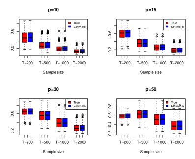
Figure 2: (a) Boxplots of $p^{-1/2}\|\widehat{\boldsymbol{\Theta}}-\boldsymbol{\Theta}\|_{F}$ of Model (4.1) with $k_{0}=5$, $r=3$ and $d_{0}=1$; (b) Boxplots of $\bar{D}(\mathcal{M}(\widehat{\mathbf{L}}_{1}),\mathcal{M}({\mathbf{L}}_{1}))$ in (4.1) with $r=3$, $k_{0}=5$ and $d_{0}=1$, where ‘True’ means we use $k_{0}$ and ‘Estimator’ corresponds using $\widehat{k}$.

Finally, we report the boxplots of $D(\mathcal{M}(\widehat{\mathbf{L}}_{1}),\mathcal{M}({\mathbf{L}}_{1}))$ in Figure 2(b). We only consider the case when $r=3$, $d_{0}=1$ and $k_{0}=5$ because the results are similar for other cases. Since $\widetilde{\mathbf{L}}$ is not an orthogonal matrix in the simulation models, we extend the discrepancy measure in (3.4) to a more general form below. Let ${\mathbf{H}}_{i}$ be a $p\times r_{i}$ matrix with rank$({\mathbf{H}}_{i})=r_{i}$, and ${\mathbf{P}}_{i}={\mathbf{H}}_{i}({\mathbf{H}}_{i}^{\prime}{\mathbf{H}}_{i})^{-1}{\mathbf{H}}_{i}^{\prime}$, $i=1,2$. Define

$$\bar{D}(\mathcal{M}({\mathbf{H}}_{1}),\mathcal{M}({\mathbf{H}}_{2}))=\sqrt{1-\frac{1}{\min{(r_{1},r_{2})}}\textrm{tr}({\mathbf{P}}_{1}{\mathbf{P}}_{2})}.$$ (4.4)

Then $\bar{D}\in[0,1]$. Furthermore, $\bar{D}(\mathcal{M}({\mathbf{H}}_{1}),\mathcal{M}({\mathbf{H}}_{2}))=0$ if and only if either $\mathcal{M}({\mathbf{H}}_{1})\subset\mathcal{M}({\mathbf{H}}_{2})$ or $\mathcal{M}({\mathbf{H}}_{2})\subset\mathcal{M}({\mathbf{H}}_{1})$, and it is 1 if and only if $\mathcal{M}({\mathbf{H}}_{1})\perp\mathcal{M}({\mathbf{H}}_{2})$. When $r_{1}=r_{2}=r$ and ${\mathbf{H}}_{i}^{\prime}{\mathbf{H}}_{i}={\mathbf{I}}_{r}$, $\bar{D}(\mathcal{M}({\mathbf{H}}_{1}),\mathcal{M}({\mathbf{H}}_{2}))$ is the same as that in (3.2). In the simulation, we take ${\mathbf{L}}_{1}=\widehat{\boldsymbol{\Sigma}}_{\eta}^{-1/2}\widetilde{\mathbf{L}}_{1}$, where $\widehat{\boldsymbol{\Sigma}}_{\eta}$ is the sample covariance matrix of $\boldsymbol{\eta}_{t}$,

From Figure 2(b), for each $p$, the discrepancy decreases as the sample increases. The effect of the estimator $\widehat{k}$ is almost negligible, especially when the sample size is large. For $p=50$, the discrepancy is smaller and less variable when $T=200$ than that when $T=500$. This is understandable because the test statistic used to determine the number of common factors $r$ tends to overestimate the true value when the dimension is high and the sample size is small. Consequently, the space $\mathcal{M}(\widehat{\mathbf{L}}_{1})$ may cover a larger space than $\mathcal{M}({\mathbf{L}}_{1})$. Overall, the simulation results are in line with the asymptotic results obtained in Section 3. In applications, to mitigate the impact of mis-identifying $r$, one can test the serial correlations of the estimated common factor associated with the $\widehat{r}$-th largest eigenvalue and adjust $\widehat{r}$ accordingly, because under the proposed model common factors are not white noise. See the two examples in the next section.

4.2 Applications

Example 1. In this example, we apply the proposed method to modeling a 15-dimensional series of $\text{PM}_{2.5}$ measurements. The original PM_2.5 data were hourly measurements at 15 monitoring stations in the southern part of Taiwan from January 1, 2006, to December 31, 2015. The locations of the 15 stations are shown in Figure 3. For simplicity, we aggregate the data to weekly observations by taking the average of measurements within each week, and then take a square-root transformation. Figure 4 shows the time plots of the transformed weekly data of the 15 stations. From Figure 4, we see clearly that the data possess strong seasonal patterns with periodicity $s\approx 52$. The plots also show certain common characteristics across the stations, but some marked differences also exist.

Figure 3: Locations (latitude versus longitude) of the 15 monitoring stations in the southern part of Taiwan around the industrial city Kaohsiung. The orders of the stations on the right legend are 14, 1, 13, 11, 9, 5, 10, 12, 8, 6, 7, 15, 3, 2, 4, respectively.

To apply the proposed method, we set $d\in\{0,1,2\}$ and $k\in\{1,...,25\}$, and found that $\widehat{d}=2$ and $\widehat{k}=3$ by the method of (2.15). Figures 5 plots the estimated trend and seasonal components of Station 1: Daliao, and the others are shown in the supplementary material because they are similar to each other. From Figure 5, we see that the $\text{PM}_{2.5}$ index was increasing from January 2006 to roughly the middle of 2009, and then decreasing after that for all 15 stations. This is because the air pollution had become a serious issue in recent years and many governments started to issue regulations to reduce the emissions after 2005. The Environmental Protection Administration in Taiwan also drew up a plan to reduce PM_2.5 pollutant starting in 2009, which resulted in a slightly decreasing trend. From Figure 5, it is clear that the measurements of the $\text{PM}_{2.5}$ are usually high during the winter and low in the summer. This is reasonable given that the measurement of $\text{PM}_{2.5}$ depends on the consumption of fossil fuels, wind direction and speed, and humidity. Winter is the dry season in Taiwan with north-west wind from the Mainland of China. On the contrary, wind is typically from the south-east (Pacific Ocean) during the summer with more rains (even typhoons). The seasonal patterns of Station 9 (Hengchun) and 10 (Meitong) are rather different from the other stations. See Figure 2 in the online supplement. This is also understandable, becuase these two stations are located at rural areas whereas the other stations are more close to the industrial city Kaohsiung. See Stations ‘9’ and ‘10’ in Figure 3.

Figure 6 presents the irregular components after removing the trend and seasonal parts. From the plots, we see that the proposed trigonometric series work well in modeling the seasonal patterns of the data. We then apply the proposed method to seek common factors in the seasonally adjusted series. For this particular instance, we chose $m=2$ for Equation (2.13). By applying the proposed test statistic to the estimated irregular components, we find that $\widehat{r}=12$, i.e. we have $12$ estimated latent common factors. Specifically, the test statistics of (2.17) and their $p$-values, in parentheses, for the first few smallest canonical correlations are 12.43(0.71), 36.11(0.37), 72.09(0.051), and 154.17(0.00). Therefore, there are three scalar components of order (0,0) among the 15 stations. The estimated transformation matrix $\widehat{\mathbf{L}}$ multiplied by 100 is shown in Equation (B.1) of the online supplement.

The time plots the 15 canonical variates and their sample autocorrelation functions are shown in the online supplement, from which we can further confirm that there are three white noise series. To model the dynamics of the whole 15 stations, we can employ a VARMA model for the selected 12 latent factors. The resulting vector structural model can then be used for prediction. It turns out a VAR(1) model is sufficient for the estimated common factor series $\widehat{{\mathbf{f}}}_{t}$. Details of the fitted model are omitted.

Figure 4: The weekly averages of the square-root-transformed PM_2.5 of 15 stations in southern Taiwan from January 2006 to December 2015 .

Figure 5: The estimated trend and seasonal components for Station 1 of the square-root-transformed PM_2.5 in southern Taiwan from January 2006 to December 2015.

Figure 6: The estimated irregular components for 15 stations of the square-root-transformed PM_2.5 in southern Taiwan from January 2006 to December 2015.

Example 2. This example considers the data of monthly value-weighted returns of 12 Industrial Portfolios, which are available at http://mba.tuck.dartmouth.edu/pages/faculty/ken.french/data_library.html. The data series span from July 1926 to May 2018 with a total of 1103 observations. The industrial sectors include the Consumer NonDurables, Consumer Durables, Manufacturing, Energy, Chemicals and Allied Products, Business Equipment, Telephone and Television Transmission, Utilities, Wholesale, Retail, and Some Services, Healthcare, Medical Equipment, and Drugs, Finance, and Others. See Figure 7 for the time plots of the data. Therefore, we have $T=1103$, $p=12$, and the periodicity $s=12$.

We first apply the proposed BIC to the data and found $\widehat{d}=0$ and $\widehat{k}=1$, that is, as expected, there is no significant trend in the data. For ease in exposition, we only show the estimated seasonal parts of the 12 industrial portfolios from January 2013 to December 2017 in Figure 8. We see that there are some monthly patterns for different portfolios. Most portfolios perform well in January and February and relatively poorly in August and September. The only exceptions are the Energy and the Utilities sectors that fare well in April and May and poorly in September and October. This effect has been documented in the literature. See Chang and Pinegar, (1989), Choi, (2008), and the references therein. There are many possible reasons. For example, the ‘January effect’ might be due to that the tax-loss selling pressures temporarily drove the security prices below their equilibrium levels in December and led to abnormal gains in the subsequent January when the pressures disappeared. Also, the study by Choi, (2008) suggests that the forward looking nature of stock prices combined with the negative economic growth in the last quarter causes the September effect, especially in the fall season when most investors become more risk averse and the stock prices reflect the future economic growth more than the rest of the year.

We apply the proposed method to the seasonally adjusted series in search of common factors. Similarly to Example 1, we also chose $m=2$ in Equation (2.13). The test statistic gives $\widehat{r}=3$, i.e. we have three estimated common factors and the rest nine transformed series are white noises. The estimated transformation matrix $\widehat{\mathbf{L}}$ multiplied by 100 and the sample autocorrelation functions of the 12 canonical variates are displayed in the online supplement, from which we further confirm that the last nine canonical variates have no significant serial correlations.

To illustrate the advantages of the proposed dimension reduction method, we compare the performance of our method with that in Lam et al. (2011) via out-of-sample prediction. For $h$-step ahead forecasts, we compare the observed and predicted returns when the models are estimated using data in the time span $[1,\tau]$ for $\tau=1002,...,1103-h$, and the $h$-step ahead forecast error is defined by

$$\text{FE}_{h}=\frac{1}{100-h+1}\sum_{\tau=1002}^{1103-h}\left(\frac{1}{\sqrt{p}}\|\widehat{\mathbf{y}}_{\tau+h}-{\mathbf{y}}_{\tau+h}\|_{2}\right),$$ (4.5)

where $p=12$ in this example. We denote GT₁ the proposed method without the seasonal adjustment, GT₂ the proposed method with seasonal adjustment, LYB the method of Lam et al. (2011), and VEC the method of applying VAR models directly to ${\mathbf{y}}_{t}$. The estimated number of common factors is $\widehat{r}=3$ for both GT₁ and GT₂ using the canonical correlation analysis, and the number of common factors obtained by the ratio-based method in Lam et al. (2011) is $\widehat{r}=1$. Then, we use VAR($d$) models, with $d$ = 1, 2, and 3, to fit the factor processes obtained by GT₁ and GT₂, and scalar AR($d$) models, with $d$ = 1, 2, and 3, to the univariate factor process obtained by LYB. For simplicity, we use AR to denote AR or VAR models, and the $h$-step ahead forecast errors are reported in Table 3 for $h=1,2$ and $3$. The smaller forecast errors are in boldface for each AR model used in the prediction and each step $h$, and similar patterns can be found for other choices of $h$. We see, from Table 3, the direct VAR models produce the worst predictions, which is due to over-parametrization when $p$ is large. Our methods GT₁ and GT₂ perform better than LYB. In particular, the seasonally adjusted method GT₂ performs slightly better than the unadjusted method GT₁. This result shows not only the advantages of the proposed dimension-reduction method, but also the necessity of seasonal adjustment.

Figure 7: Monthly value-weighted returns of 12 industrial portfolios from July 1926 to May 2018. They are 1. Consumer NonDurables; 2. Consumer Durables; 3. Manufacturing; 4. Energy; 5. Chemicals and Allied Products; 6. Business Equipment; 7. Telephone and Television Transmission; 8. Utilities; 9. Wholesale, Retail, and Some Services; 10. Healthcare, Medical Equipment, and Drugs; 11. Finance; 12. Other.

Figure 8: Estimated seasonal components of 12 industrial portfolios from January 2013 to December 2017. They are 1. Consumer NonDurables; 2. Consumer Durables; 3. Manufacturing; 4. Energy; 5. Chemicals and Allied Products; 6. Business Equipment; 7. Telephone and Television Transmission; 8. Utilities; 9. Wholesale, Retail, and Some Services; 10. Healthcare, Medical Equipment, and Drugs; 11. Finance; 12. Other.

Table 3: The 1-step, 2-step and 3-step ahead forecasting errors. Standard errors are given in the parentheses. GT₁ denotes the proposed method without the seasonal part, GT₂ denotes the proposed method with seasonal adjustment, ‘LYB’ is the one in Lam et al. (2011), and VEC denotes the direct vector AR method.

		GT1	GT2	LYB	VEC
$1$-step	AR(1)	3.86 (2.07)	3.86 (2.09)	3.87 (2.08)	3.97 (2.08)
	AR(2)	3.87 (2.07)	3.87 (2.09)	3.88 (2.05)	4.01 (2.05)
	AR(3)	3.90 (2.06)	3.89 (2.07)	3.91 (2.06)	4.05 (2.01)
$2$-step	AR(1)	3.80 (2.03)	3.79 (2.04)	3.82 (2.03)	3.82 (2.04)
	AR(2)	3.80 (2.03)	3.79 (2.02)	3.82 (2.01)	3.84 (1.97)
	AR(3)	3.83 (2.02)	3.81 (2.01)	3.85 (1.99)	3.89 (1.97)
$3$-step	AR(1)	3.81 (2.03)	3.80 (2.03)	3.83 (2.03)	3.85 (2.04)
	AR(2)	3.81 (2.03)	3.80 (2.03)	3.83 (2.03)	3.84 (2.03)
	AR(3)	3.83 (2.01)	3.82 (2.02)	3.85 (2.02)	3.91 (2.00)

5 Concluding Remark

In this paper, we proposed a structural-factor approach for high-dimensional time series analysis and demonstrated its applications with a 15-dimensional series of weekly PM_2.5 and the monthly value-weighted returns of 12 U.S. Industrial Portfolios. For the PM_2.5 data, we do not consider explicitly the spatial structure of the monitoring stations. One can treat the proposed model as a specification for the dynamic dependence of the conditional mean, which can be augmented with a spatial covariance specification, if needed. Such an extension would be useful, especially if one is interested in predicting the PM_2.5 at a location not far away from the monitoring stations. In the Industrial Portfolios data, the proposed method suggests a substantial dimension reduction and produces more accurate out-of-sample forecasts.

Supporting Information

The supplementary material contains all technical proofs of the theorems in Section 3 and some additional Tables and Figures of the real examples of Section 4.

Data Availability Statement

The PM_2.5 data used in Example 1 are available in the online Supporting Information file: weekly-TaiwanSouth-PM25.csv. The data used in Example 2 are available at the website cited.

References

- Anderson (1958) Anderson TW. 1958. An Introduction to Multivariate Statistical Analysis. Wiley, New York.
- Bai and Ng (2002) Bai J, Ng S. 2002. Determining the number of factors in approximate factor models. Econometrica 70: 191–221.
- Barsky and Miron, (1989) Barsky RB, Miron JA. 1989. The seasonal cycle and the business cycle. Journal of Political Economy 97: 503–-534.
- Box and Tiao (1977) Box GEP, Tiao GC. 1977. A canonical analysis of multiple time series. Biometrika 64: 355–365.
- Chang and Pinegar, (1989) Chang EC, Pinegar JM. 1989. Seasonal fluctuations in industrial production and stock market seasonals. Journal of Financial and Quantitative Analysis 24(1): 59–74.
- Chang et al., (2015) Chang J, Guo B, Yao Q. 2015. High dimensional stochastic regression with latent factors, endogeneity and nonlinearity. Journal of Econometrics 189(2): 297–312.
- Chang et al., (2009) Chang Y, Miller JI, Park JY. 2009 Extracting a common stochastic trend: Theory with some applications. Journal of Econometrics 150(2): 231–247.
- Choi, (2008) Choi HS. 2008. Three essays on stock market seasonality. PhD diss., Georgia Institute of Technology,
- Davis et al. (2012) Davis RA, Zang P, Zheng T. 2012. Sparse vector autoregressive modelling. Available at arXiv:1207.0520.
- De livera et al., (2011) De Livera AM, Hyndman RJ, Snyder RD. 2011. Forecasting time series with complex seasonal patterns using exponential smoothing. Journal of the American Statistical Association 106(496): 1513–1527.
- Forni and Lippi, (1997) Forni M, Lippi M. 1997. Aggregation and the Microfoundations of Dynamic Macroeconomics. Oxford University Press.
- Gao et al. (2018) Gao Z, Ma Y, Wang H, Yao Q. 2019. Banded spatio-temporal autoregressions. Journal of Econometrics 208: 211–230.
- Guo et al. (2016) Guo S, Wang Y, Yao Q. 2016. High dimensional and banded vector autoregression. Biometrika 103(4): 889–903.
- Harvey, (1989) Harvey AC. 1989. Forecasting, Structural Time Series Models and the Kalman Filter. Cambridge University Press, Cambridge, UK.
- Harvey and Koopman, (1993) Harvey A, Koopman SJ. 1993. Forecasting hourly electricity demand using time-varying splines. Journal of the American Statistical Association 88(424): 1228–1236.
- Kelejian and Prucha (2010) Kelejian HH, Prucha IR. 2010. Specification and estimation of spatial autoregressive models with autoregressive and heteroskedastic disturbances. Journal of Econometrics 157: 53–67.
- Lam and Yao, (2012) Lam C, Yao Q. 2012. Factor modeling for high-dimensional time series: inference for the number of factors. The Annals of Statistics 40(2): 694–726.
- Lam et al. (2011) Lam C, Yao Q, Bathia N. 2011. Estimation of latent factors for high-dimensional time series. Biometrika 98: 901–918.
- Lee and Yu (2010) Lee LF, Yu J. 2010. Some recent developments in spatial panel data models. Regional Science and Urban Economics 40: 255–271.
- Lin and Lee (2010) Lin X, Lee LF. 2010. GMM estimation of spatial autoregressive models with unknown heteroskedasticity. Journal of Econometrics, 177: 34–52.
- Luo and Chen, (2013) Luo S, Chen Z. 2013. Extended BIC for linear regression models with diverging number of relevant features and high or ultra-high feature spaces. Journal of Statistical Planning and Inference 143: 494-–504.
- Lütkepohl, (2006) Lütkepohl H. 2006. New Introduction to Multiple Time Series Analysis, Springer, Berlin.
- Nerlove, (1964) Nerlove M. 1964. Spectral analysis of seasonal adjustment procedures. Econometrica 32: 241–286.
- Pan and Yao, (2008) Pan J, Yao Q. 2008. Modelling multiple time series via common factors. Biometrika 95(2): 365–379.
- Peña and Poncela, (2006) Peña D, Poncela P. 2006. Nonstationary dynamic factor analysis. Journal of Statistical Planning and Inference 136(4): 1237–1257.
- Plosser, (1979) Plosser CI. 1979. The analysis of seasonal economic models. Journal of Econometrics 10(2): 147–-163.
- Shojaie and Michailidis (2010) Shojaie A, Michailidis G. 2010. Discovering graphical Granger causality using the truncated lasso penalty. Bioinformatics 26: 517–523.
- Song and Bickel (2011) Song S, Bickel PJ. 2011. Large vector auto regressions. Available at arXiv:1106.3519.
- Stock and Watson (2002) Stock JH, Watson MW. 2002. Forecasting using principal components from a large number of predictors. Journal of the American Statistical Association 97: 1167–1179.
- Stock and Watson (2005) Stock JH, Watson MW. 2005. Implications of dynamic factor models for VAR analysis. Available at www.nber.org/papers/w11467.
- Su (2012) Su, L. 2012. Semiparametric GMM estimation of spatial autoregressive models. Journal of Econometrics, 167, 543–560.
- Tiao and Tsay (1989) Tiao GC, Tsay RS. 1989. Model specification in multivariate time series (with discussion). Journal of the Royal Statistical Society: Series B (Statistical Methodology) 51: 157–213.
- Tsay (2014) Tsay RS. 2014. Multivariate Time Series Analysis. Wiley, Hoboken, NJ.
- Wallis, (1978) Wallis KF. 1978. Seasonal adjustment and multiple time series analysis (with discussion). In Seasonal Analysis of Economic Time Series, ed. Arnold Zellner. 347–364.
- Yu et al. (2008) Yu J, De Jong R, Lee LF. 2008. Quasi-maximum likelihood estimators for spatial dynamic panel data with fixed effects when both and are large. Journal of Econometrics 146: 118–134.
- Zhang et al. (2015) Zhang YJ, Yi WC, Li BW. 2015. The impact of urbanization on carbon emission: empirical evidence in Beijing. Energy Procedia 75: 2963–2968.
- dataset (2018) Dataset. 2018. http://mba.tuck.dartmouth.edu/pages/faculty/ken.french/data_library.html.