Single-View Place Recognition under Seasonal Changes

Abstract

Single-view place recognition, that we can define as finding an image that corresponds to the same place as a given query image, is a key capability for autonomous navigation and mapping. Although there has been a considerable amount of research in the topic, the high degree of image variability (with viewpoint, illumination or occlusions for example) makes it a research challenge.

One of the particular challenges, that we address in this work, is weather variation. Seasonal changes can produce drastic appearance changes, that classic low-level features do not model properly. Our contributions in this paper are twofold. First we pre-process and propose a partition for the Nordland dataset, frequently used for place recognition research without consensus on the partitions. And second, we evaluate several neural network architectures such as pre-trained, siamese and triplet for this problem. Our best results outperform the state of the art of the field. A video showing our results can be found in https://youtu.be/VrlxsYZoHDM. The partitioned version of the Nordland dataset at http://webdiis.unizar.es/~jmfacil/pr-nordland/.

I Introduction

Visual place recognition consists on, having a query image, retrieving from a database another image that corresponds to the same place, see Fig. 1. Place recognition plays a relevant role in several applications, e.g. mobile robotics. To name a few, place recognition can be used for topological mapping [1], for loop closure and drift removal in geometric mapping [2], and for learning scene dynamics in lifelong localization and mapping [3].

Place recognition for robotics presents multiple challenges. For example, most of the times the places databases are huge and the retrieval time is constrained by the real-time operation of robots. Another relevant challenge, which is the one we will address in this paper, is the variability in the visual appearance of the places. The appearance variations might have different sources: viewpoint and illumination changes, occlusions and scene dynamics.

The appearance changes coming from different viewpoints and illumination conditions, assuming a static scene, have been addressed quite successfully. Local point features (e.g., SIFT, SURF and ORB), based on image gradients, show a high repeatability and descriptor invariance to moderate levels of illumination and viewpoint changes. Checking the geometric and sequential compatibility of such local features can improve even further their robustness [4]. Global image features have been also used for place recognition [5, 6], showing better scalability but lower performance under viewpoint changes or occlusions.

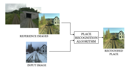
Figure 1: Place recognition overview. The inputs are two; a database of images taken in different places, and query view imaging the place to recognize. The output is an image of the database showing the place of the query image.

The classical approaches based on hand-designed low-level features are, however, limited for the representation of dynamic scene changes. There has been several works aiming at designing descriptors with higher invariance to certain transformations, either based on models (e.g., [7]) or based on learning from data (e.g., [8]). The most recent approaches use Convolutional Neural Networks (CNNs), due to their higher potential to learn image patterns. In this work we explore the use of CNNs for place recognition in the particular case of seasonal changes. Our specific contributions over the state of the art are:

• We have trained a weather-invariant place recognition method, based on CNNs. We use CNNs to extract image descriptors, that we compare using the Euclidean distance. Fig. 2 depicts some of the weather variations considered.

• We have designed a dataset using images extracted from the Nordland videos [9]. We propose our Nordland dataset partition as a common framework for evaluating place recognition.

• We have compared our results in the Nordland dataset against other state of the art techniques. Our method is capable of correctly recognizing $98\%$ of the input places in $80$km routes under favorable conditions and $86\%$ under drastic appearance changes like the ones occurring between summer and winter.

The rest of this paper is structured as follows. Section II analyzes the related work in place recognition. Section III explains the development of the dataset. Section IV introduces the neural network architectures that we have used. Section V presents our results. Finally, in section VI we summarize our conclusions.

Figure 2: Images from the same place in different seasons. From top-left and clockwise: winter, summer, fall and spring. Notice the appearance change due to different weather conditions. The images have been extracted from the videos of the Nordland dataset.

II Related work

The most common approaches to place recognition are based on local image features using classic extractors and descriptors. Two of the most relevant among these techniques are FAB-MAP [10] and DBoW [4]. The performance of these algorithms is excellent for moderate viewpoint and illumination changes, but it decreases for other types of appearance variations.

An alternative approximation consists in using neural networks as feature extractors. Sünderhauf et al. analyzed in [11] the use of neural networks for the purpose of place recognition with promising results. [11, 12] and [13] were the first ones to use neural networks for this purpose but [14] and [15] were the first ones to specifically train neural architectures to attack this problem. There is no consensus on what kind of architecture is better for this task.

In this work we compare three different techniques that can be considered state of the art in place recognition: Unsupervised linear learning techniques for visual place recognition [16], deep learning features at scale for visual place recognition [15] and CNN for appearance-invariant place recognition [14].

The first method [16] applied principal components analysis to reduce the dimensionality of the feature vector, eliminating the dimensions that are affected by appearance changes. The second method [14] used a triplet neural network architecture to fine-tune a pre-trained model and improve the robustness of the extracted features. Their network learned to map images to a vector space where euclidean distance represents similarity. The third method [15] trained a deep neural network to classify the place that appeared in a dataset of images taken from surveillance cameras.

This work develops a technique similar to the one implemented in [14]. As a novelty, we also train siamese neural networks and consider different pre-trained networks.

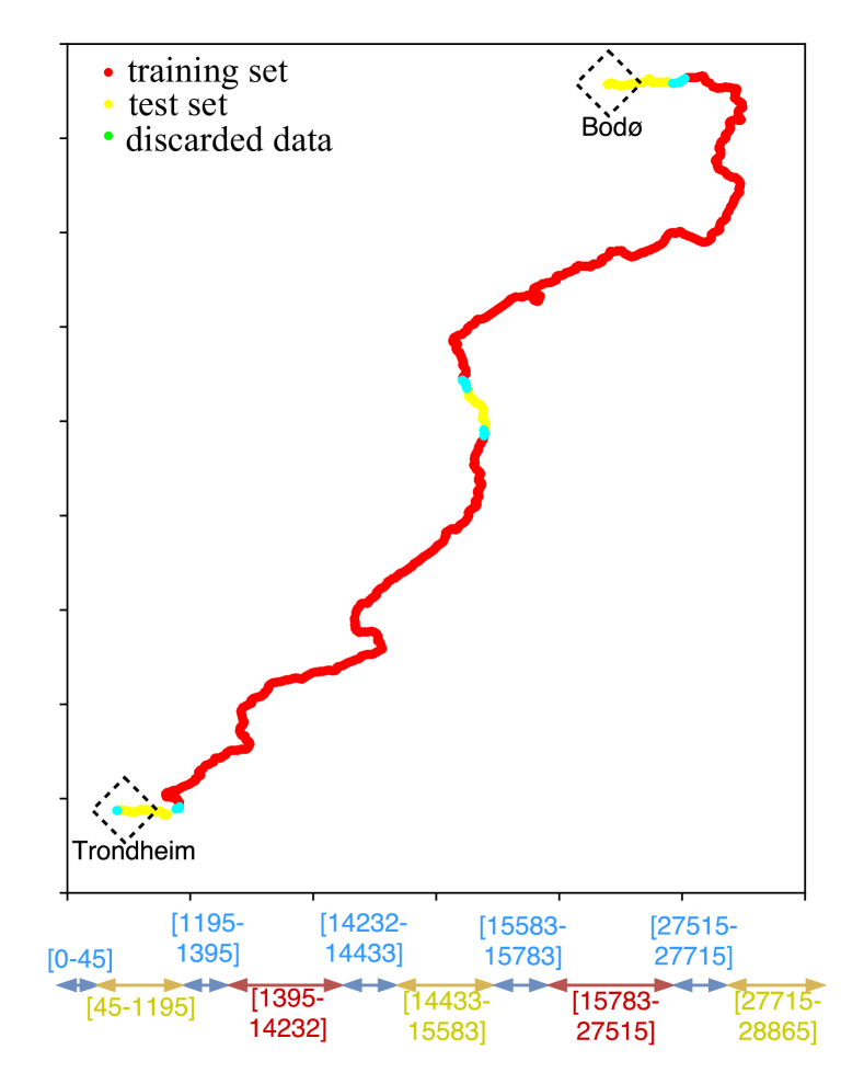
Figure 3: Proposed dataset partition for the Nordland dataset. Top: Geographical representation of the training (red) and test (yellow) sets. Bottom: Index representation of the distribution, w.r.t. frame index in the videos.

III The Nordland Dataset: Pre-Processing and Partitions

In this work, we have used the Nordland railroad videos. In 2012, the Norway broadcasting company (NRK) made a documentary about the Nordland Railway, a railway line between the cities of Trondheim and Bodø. They filmed the $729$km journey with a camera in the front part of the train in winter, spring, fall and summer. The length of each video is about 10 hours and each frame is timestamped with the GPS coordinates.

This dataset has been used by other research groups in place recognition, for example [14] and [16]. Each group uses different partitions for training and test, making difficult to reproduce the results. In this work we propose a specific partition of the dataset and a baseline, to guarantee a fair comparison between algorithms. Our intention is to release the processed dataset if the paper is accepted.

III-A Data pre-processing

The first step, creating the dataset, was to extract the maximum number of images from each video. Moreover, GPS data corruption was fixed and we also eliminated tunnels and stations. After these steps, grabbing one frame per second, we obtained $28,865$ images per video. We used speed information from the GPS data to filter stations and a darkness threshold to filter tunnels.

III-B Dataset partitions

Fig. 3 illustrates the partition of the whole image set in the Nordland dataset. We decided to create the test set with three different sequences of $1,150$ images (a total of $3,450$, yellow in the figure). The rest of the images were used for training ($24,569$, red in the figure). By using multiple sections, the variety of places and appearance changes contained in the test set increases. We also left a separation of a few kilometers between each test and train section by discarding some images in order to guarantee the difference between test and train data.

III-C Place labels

Given the similarity between consecutive images, in this work we propose to consider that two images are of the same place if temporally they are separated by $3$ images or less. We applied a sliding window of $5$ images over the whole dataset in order to group images taken from five consecutive seconds. This process can be seen in Fig. 4.

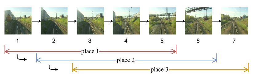
Figure 4: A sliding window of five images is considered in this work as the same place. Notice the similarity of consecutive images. The figure is best viewed in electronic format.

IV Neural network architectures

Fig. 5 shows the functional blocks of the proposed place recognition method. Our goal was to train a network to extract feature vectors that are close to the ones extracted from images of the same place, even in the presence of appearance changes. Our similarity metric is the Euclidean distance. We acknowledge that the distance function plays an important role in the feature space distribution, loss and optimization convergence. However, we preferred to focus our efforts on other parts of the problem rather than experimenting with other alternatives, e.g., the cosine distance.

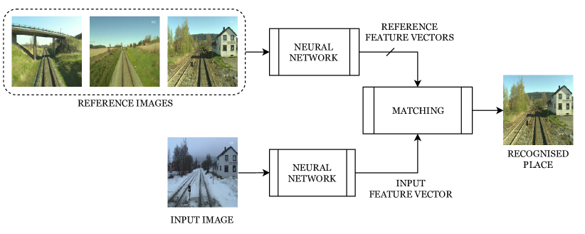
Figure 5: Overview of the place recognition algorithm. First, we extract a descriptor for every (visited place) image in the database. Second, for every new image (query) we extract its descriptor and compare it with those extracted from the database. The retrieved place will be the one with the most similar descriptor.

We studied three different ways of using neural networks. First of all, we evaluated the performance of features extracted by pre-trained networks. We then proceeded to train siamese and triplet architectures specifically for the problem of place recgonition.

IV-A Pre-trained networks

In [11], Sünderhauf et al. studied the performance of features from different neural networks for the purpose of place recognition. In this work, we analyzed the features extracted by some layers of the popular VGG-16 model [17], which was trained on Imagenet. Fig. 6 shows the structure of the model and the layers that we have evaluated. We have also evaluated the performance of the same architecture trained for scene recognition on the Places dataset.

In the rest of this paper, by extracted feature vector we refer to the output of the neural network at the chosen layer after the non-linear activation. In the case of convolutional layers, we flattened the output tensor.

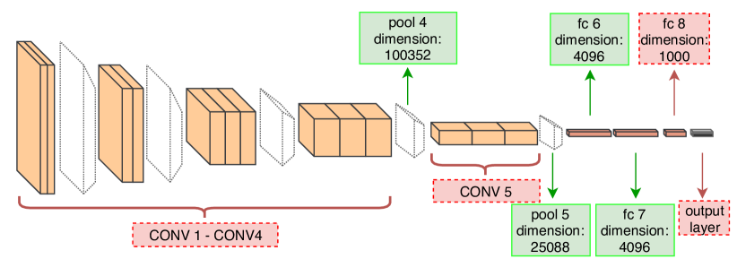
Figure 6: VGG-16 Layers. In red: Layers not used. In green: Used layers.

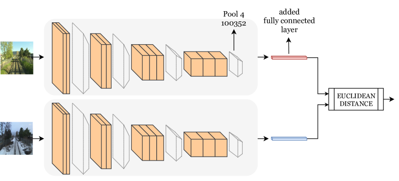
Figure 7: Siamese architecture used in our work. We show in gray the pre-trained CNN blocks. The fully-connected layer added has $128$ neurons.

IV-B Siamese networks

Siamese neural networks, proposed in [18], are capable of improving the robustness of pre-trained descriptors for place recognition. We modified the VGG-16 model in order to use a siamese architecture and added a new fully-connected layer (without activation function) after the one that showed the best performance in the pre-trained experiments. The final structure is showed in Fig. 7. Training was done for $5$ epochs with $834,746$ positive pairs (two images of the same place with different appearance) and $834,746$ negative pairs (two images of different places) taken from the previously mentioned training dataset. We used the contrastive loss [19].

IV-C Triplet networks

As mentioned in Section II, Gómez-Ojeda et al. [14] were the first ones to train triplet networks with this purpose. Triplet neural networks improve the results of siamese architectures by training positive and negative pairs at the same time. Moving closer the descriptors from the same place and apart the descriptors from different places in the same instant leads to a more stable and efficient learning process.

In order to use a triplet architecture, we modified the VGG-16 pre-trained model by adding a new fully-connected layer (without activation function) after the layer that performed better in the pre-trained experiments. We trained the new layer with $834,746$ image triplets for $5$ epochs. The loss function used in this case was the Wohlhart-Lepetit loss. This loss, proposed in [20] was also used in [14]:

$$E=max\left\{0,1-\frac{d_{n}}{margin+d_{p}}\right\}$$ (1)

Where $E$ is the loss error, $d_{p}$ is the distance between the positive and neutral input, $d_{n}$ is the distance between the neutral and negative input and $margin$ is a parameter that limits the difference between the distances.

In this function, the loss is zero when the positive pair is closer than the negative pair plus the margin. Moreover, the loss value is limited between 0 and 1. We set the margin value to 1 in all our experiments.

V Experimental Results

In order to evaluate our deep models, we used the images from one season as reference and images of a different season as query (summer against winter, winter against fall, etc.). Each image is processed by the neural network to produce the feature vector. After the extraction, each feature vector is compared with every feature vector of every reference season, and the closest one is considered the place predicted by the algorithm. This process is repeated for each one of the $3,450$ test images. The number of times that the closest place is the correct one gives the the fraction of correct matches fc, which is the metric that we have used.

$$\text{fc}=\frac{\text{\# of correct predicted places}}{\text{\# of evaluated places}},$$ (2)

It is important to note that we consider a match is correct when the closest feature vector corresponds to a place within a $5$-frames window. The distance between the feature vectors measures the confidence of the result and a distance threshold can be applied to obtain precision-recall curves. We have preferred to focus our analysis on the robustness of the extracted features.

V-A Pre-trained

Fig. 8 shows the results obtained from the original VGG-16 pre-trained model. Out of all the studied layers, we found that features extracted from the fourth pooling layer (pool4) had the highest fraction of correct matches in all the season combinations. The results are worse as the layers are closer to the VGG-16 output. The main reason might be that, as the dimension of the layer decreases, some of the information that is robust to appearance changes is lost. Moreover, the last layers of the model contain semantic information which is specific to the original problem.

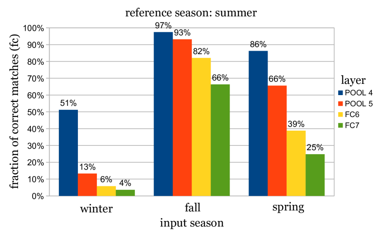
Figure 8: Fraction of correct matches using the pre-trained VGG-16 layers as feature extractors with summer as reference season and the other seasons as input.

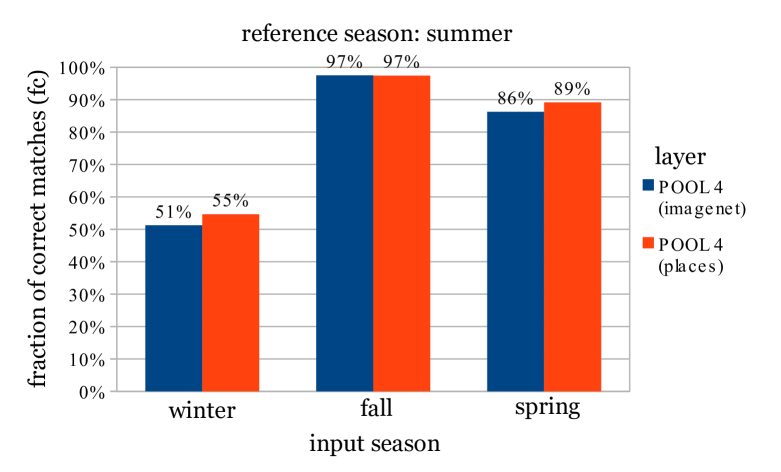
Figure 9: Fraction of correct matches using features from the pool4 layer of VGG-16. We compare the Imagenet pre-trained version vs the Places dataset pre-trained one. We show the results with summer as reference season and the other seasons as input.

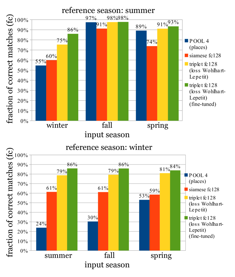
Figure 10: Fraction of correct matches using different strategies: Pre-trained, siamese and triplet networks (with and without fine-tuning). Top: Results with summer as reference season and the other seasons as input. Bottom: Results with winter as reference season and the other seasons as input.

After that, we compared the performance of the original VGG-16 model to the VGG-16 model trained on the Places dataset by evaluating the features extracted from the pool4 layer. We observed that the model trained for scene-recognition achieved better results in all the studied combinations, as shown in Fig. 9. The main reason behind this is that, in order to classify scenes, the internal layers of the model have learned to extract features that are more useful for place recognition.

In the rest of our experiments, we decided to use the fourth pooling layer of the VGG-16 trained on the Places dataset as the starting point. The extracted feature vectors have a dimension of $100,352$.

V-B Siamese and triplets

After several experiments, we observed that a descriptor size of $128$ is sufficiently discriminative for place recognition. Increasing the size of the layer increases the computational cost without a significant improvement in the accuracy.

Fig. 10 compares the results obtained with the pre-trained, siamese and triplet architectures. The pre-trained network only outperformed the siamese architecture in some combinations where summer images were used as reference. It should be noted that the siamese feature vector has $128$ dimensions, while the pre-trained one has $100,352$. Even if the siamese network has not outperformed all the pre-trained results, the siamese architecture has learnt to extract a much smaller feature vector, while keeping the discriminative information.

On the other hand, the triplet network outperformed the siamese and pre-trained models in all the studied combinations. The triplet results that we show in Fig. 10, belong to two different experiments. In our first experiments, we trained the newly added layer (triplet fc128 - loss Wohlhart Lepetit). We then proceeded to train the layer while fine-tuning the rest of the VGG-16 pre-trained structure (triplet fc128 - loss Wohlhart Lepetit - fine-tuned). It can be observed that the accuracy of the fine-tuned model is higher.

We conclude that the best results were obtained with the fine-tuned triplet network, starting from the weights of the pre-trained VGG-16-Places and adding a fully-connected layer with an output dimension of $128$.

Table I shows the fraction of correct matches achieved for every possible combination of reference-input seasons.

TABLE I: Fraction of correct matches for every season combination.

input \reference	summer	fall	winter	spring
summer	—	0.8548	0.8591	0.9545
fall	0.9777	—	0.8583	0.9562
winter	0.8597	0.9771	—	0.9545
spring	0.9336	0.94	0.8388	—

V-C Comparison against other approaches

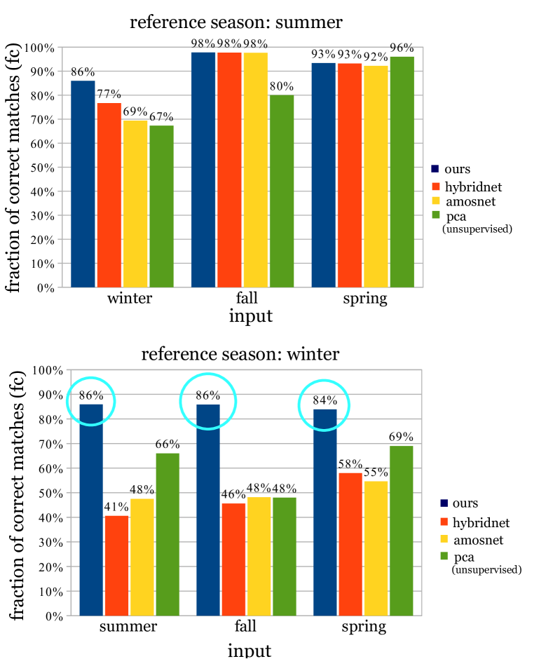
Figure 11: Fraction of correct matches comparison: our work, Hybridnet, Amosnet and the unsupervised PCA technique. Top: Results with summer as reference season and the other seasons as input. Bottom: Results with winter as reference season and the other seasons as input.

Fig. 11 shows the comparison between our results, the PCA technique of [16] and the two neural network models trained in [15] (Hybridnet and Amosnet). The comparison is made using summer and winter as the reference seasons. Notice that our model matches or outperforms the other techniques in almost every combination, and particularly in those with drastic appearance changes. In the most challenging cases (the ones with winter as reference) the best result is obtained with summer and fall as input seasons, where our model achieved 86% of correct matches while the second best, the unsupervised PCA [16], obtained less than 66%.

The unsupervised PCA results were obtained from their original paper [16]. For Hybridnet and Amosnet, we downloaded the models from the authors of [15] and tested their performance in the test partition of our dataset.

Finally, Fig. 12 shows two examples of correct matches. Notice that our method is robust to strong changes produced by snow and illumination. Fig. 13 shows two examples of incorrect matches. Notice that both are difficult even for a human. The similarities in the geographical features of those places make them look like the same place.

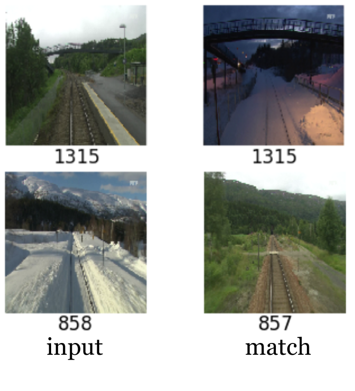
Figure 12: Places correctly recognized by our algorithm. The index in the sequence is shown at the bottom of each image.

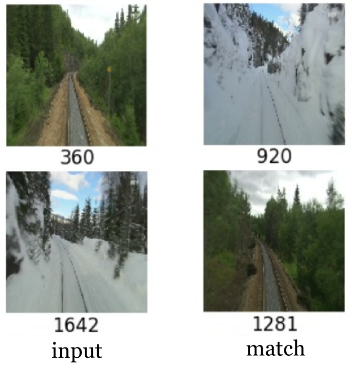
Figure 13: False positive examples from our algorithm. The index in the sequence is shown at the bottom of each image. Notice that these particular places are difficult even for a human.

VI Conclusions

In this work we have implemented a place recognition method which is robust to appearance changes, in particular to those caused by weather conditions. Our proposal works by training a neural network to extract a descriptor, that can be compared with others using the Euclidean distance.

Our experiments show that siamese and triplet neural networks learn robust features to appearance changes. Triplet neural networks achieved better results than siamese ones. We show that a VGG-16 model trained on the Places dataset shows a reasonable performance, improved by fine-tuning. Finally, we have shown that our method achieves state-of-the-art results in place recognition on the Nordland dataset.

References

- [1] E. Garcia-Fidalgo and A. Ortiz, “Hierarchical place recognition for topological mapping,” IEEE Transactions on Robotics, vol. 33, no. 5, pp. 1061–1074, 2017.
- [2] R. Mur-Artal, J. M. M. Montiel, and J. D. Tardos, “Orb-slam: a versatile and accurate monocular slam system,” IEEE Transactions on Robotics, vol. 31, no. 5, pp. 1147–1163, 2015.
- [3] M. Dymczyk, S. Lynen, T. Cieslewski, M. Bosse, R. Siegwart, and P. Furgale, “The gist of maps-summarizing experience for lifelong localization,” in Robotics and Automation (ICRA), 2015 IEEE International Conference on, pp. 2767–2773, IEEE, 2015.
- [4] D. Gálvez-López and J. D. Tardos, “Bags of binary words for fast place recognition in image sequences,” IEEE Transactions on Robotics, vol. 28, no. 5, pp. 1188–1197, 2012.
- [5] N. Sünderhauf and P. Protzel, “Brief-gist-closing the loop by simple means,” in Intelligent Robots and Systems (IROS), 2011 IEEE/RSJ International Conference on, pp. 1234–1241, IEEE, 2011.
- [6] A. C. Murillo, G. Singh, J. Kosecká, and J. J. Guerrero, “Localization in urban environments using a panoramic gist descriptor,” IEEE Transactions on Robotics, vol. 29, no. 1, pp. 146–160, 2013.
- [7] E. Simo-Serra, C. Torras, and F. Moreno-Noguer, “Dali: deformation and light invariant descriptor,” International journal of computer vision, vol. 115, no. 2, pp. 136–154, 2015.
- [8] Y. Verdie, K. Yi, P. Fua, and V. Lepetit, “Tilde: A temporally invariant learned detector,” in Proceedings of the IEEE Conference on Computer Vision and Pattern Recognition, pp. 5279–5288, 2015.
- [9] N. B. Corporation, “Nordlandsbanen: minute by minute, season by season,” 2012. [Online; accessed 19-June-2017].
- [10] M. Cummins and P. Newman, “Fab-map: Probabilistic localization and mapping in the space of appearance,” The International Journal of Robotics Research, vol. 27, no. 6, pp. 647–665, 2008.
- [11] N. Sünderhauf, F. Dayoub, S. Shirazi, B. Upcroft, and M. Milford, “On the performance of convnet features for place recognition,” CoRR, vol. abs/1501.04158, 2015.
- [12] P. Neubert and P. Protzel, “Local region detector+ cnn based landmarks for practical place recognition in changing environments,” in Mobile Robots (ECMR), 2015 European Conference on, pp. 1–6, IEEE, 2015.
- [13] A. Gout, Y. Lifchitz, T. Cottencin, Q. Groshens, S. Griffith, J. Fix, and C. Pradalier, Evaluation of off-the-shelf cnns for the representation of natural scenes with large seasonal variations. PhD thesis, UMI 2958 GeorgiaTech-CNRS; CentraleSupélec UMI GT-CNRS 2958 Université Paris-Saclay, 2017.
- [14] R. Gomez-Ojeda, M. Lopez-Antequera, N. Petkov, and J. Gonzalez-Jimenez, “Training a convolutional neural network for appearance-invariant place recognition,” arXiv preprint arXiv:1505.07428, 2015.
- [15] Z. Chen, A. Jacobson, N. Sunderhauf, B. Upcroft, L. Liu, C. Shen, I. Reid, and M. Milford, “Deep learning features at scale for visual place recognition,” arXiv preprint arXiv:1701.05105, 2017.
- [16] S. Lowry and M. J. Milford, “Supervised and unsupervised linear learning techniques for visual place recognition in changing environments,” IEEE Transactions on Robotics, vol. 32, no. 3, pp. 600–613, 2016.
- [17] K. Simonyan and A. Zisserman, “Very deep convolutional networks for large-scale image recognition,” arXiv preprint arXiv:1409.1556, 2014.
- [18] J. Bromley, I. Guyon, Y. LeCun, E. Säckinger, and R. Shah, “Signature verification using a” siamese” time delay neural network,” in Advances in Neural Information Processing Systems, pp. 737–744, 1994.
- [19] R. Hadsell, S. Chopra, and Y. LeCun, “Dimensionality reduction by learning an invariant mapping,” in Computer vision and pattern recognition, 2006 IEEE computer society conference on, vol. 2, pp. 1735–1742, IEEE, 2006.
- [20] P. Wohlhart and V. Lepetit, “Learning descriptors for object recognition and 3d pose estimation,” in Proceedings of the IEEE Conference on Computer Vision and Pattern Recognition, pp. 3109–3118, 2015.