Bifurcations to turbulence in transitional channel flow

Abstract

In wall-bounded parallel flows, sustained turbulence can occur even while laminar flow is still stable. Channel flow is one of such flows and displays spatio-temporal fluctuating patterns of localized turbulence along its way from/to featureless turbulence. By direct numerical simulation, we study the observed inconsistency between turbulence decay according to a two-dimensional directed-percolation ($2D$-DP) scenario and the presence of sustained oblique localized turbulent bands (LTBs) below the DP critical point. Above Reynolds number $\mathrm{Re}_{\rm g}\sim 700$ sustained LTBs are observed; most LTBs have the same orientation so that the spanwise symmetry of the LTB pattern is broken below $\mathrm{Re}_{2}\sim 1000$. The frequency of transversal splitting, by which an LTB generates another one with opposite obliqueness, so that turbulence spreading becomes intrinsically two dimensional, increases in the range $\mathrm{Re}_{\rm g}<\mathrm{Re}<\mathrm{Re}_{2}$. It reaches a critical rate at $\mathrm{Re}_{2}$ beyond which symmetry is restored. $2D$-DP behavior is retrieved only above $\mathrm{Re}_{2}$. A mean-field model is proposed which qualitatively accounts for the above symmetry-restoring bifurcation by considering interactions between space-averaged densities of LTBs propagating in either direction.

I Introduction

The ways shear flows become turbulent markedly depend on the shape of their laminar velocity profiles and the occurrence of instability mechanisms of Kelvin–Helmholtz type affecting them. Inflectional profiles like in free shear layer, wakes, or jets, become unstable at rather low values of the Reynolds number against such modes of inertial origin and then turn turbulent through a continuous cascade of successive instabilities Huerre and Rossi (1998), each step being in principle captured by weakly nonlinear perturbation theory, resulting in a globally supercritical transition to turbulence. By contrast, unidirectional flows controlled by the shear at solid walls do not display inflection points and are not prone to such instability modes. They may become unstable but only against more intricate and counter-intuitive mechanisms involving viscous dissipation Huerre and Rossi (1998); Schmid and Henningson (2012). The so-produced Tollmien–Schlichting waves develop only at high Reynolds number, beyond a certain linear threshold $\mathrm{Re}_{\rm c}$ (later denoted $\mathrm{Re}_{\rm TS}$ for convenience). Pipe flow in tubes of circular and square sections or plane Couette flow between flat counter-translating plates remain linearly stable for all $\mathrm{Re}$, $\mathrm{Re}_{\rm c}\to\infty$, whereas for channel flow (plane Poiseuille flow) $\mathrm{Re}_{\rm c}<\infty$ Orszag (1971). For such flows the transition is globally subcritical. Physically infinitesimal perturbations are however not mathematically infinitesimal but only finite-but-small, and the possibility of a direct transition to turbulence, called bypass, is in practice observed at moderate values of $\mathrm{Re}$ due to the nonlinearity of the Navier–Stokes equations: At increasing $\mathrm{Re}$ the flow can in principle be maintained steady and laminar up to $\mathrm{Re}_{\rm c}\leq\infty$, but the introduction of finite perturbations with particular shapes and amplitudes may force it to become unsteady. There is therefore a full range of Reynolds numbers, called transitional, where the trivial laminar solution coexists with other nontrivial solutions. These solutions are usually chaotic and cannot be straightforwardly reached by standard perturbation analysis. A direct transition to turbulence is observed with strong hysteresis upon continuous up-and-down variation of $\mathrm{Re}$, the flow jumping from the laminar solution branch to the nontrivial turbulent branch or back. Once in a state belonging to the nontrivial branch, the flow can be maintained turbulent down to a global stability threshold $\mathrm{Re}_{\rm g}$ below which the only possible stable regime is laminar.

Sub-criticality is often perceived as a problem to be studied within the theory of dynamical systems. Solutions to the Navier–Stokes equations are then searched under minimal flow unit (MFU) conditions Jiménez and Moin (1991) with periodic boundary conditions at short distances, focusing on coherent structures analyzed in the corresponding phase space perspective Waleffe (2001); Kawahara et al. (2012). This approach was progressively generalized to deal with extended systems in one or two in-plane directions, and mostly concentrated on the existence and properties of isolated localized solutions at the edge of chaos, see e.g. Zammert and Eckhardt (2014) for channel flow. On the other hand, when appreciated in physical space, provided that the system’s geometry is wide enough, states along the nontrivial branch in general display a coexistence of domains alternately laminar and turbulent separated by fluctuating interfaces.

In a number of cases, beyond $\mathrm{Re}_{\rm g}$ this laminar-turbulent coexistence happens in the form of a regular pattern. The iconic case is that of the turbulent spiral obtained in moderate-gap cylindrical Couette flow by Coles Coles (1965), and re-obtained later by Andereck et al. Andereck et al. (1986) who introduced the term featureless to qualify the regime obtained at higher shearing rates when turbulence has apparently returned to statistical uniformity. In small-gap experiments, several helical branches were obtained Prigent et al. (2003). Close to the featureless regime, laminar-turbulent patterning involved superpositions of such helices with opposite pitch while, plane Couette flow being understood as the zero-curvature limit of cylindrical Couette flow, helices were straightened into oblique bands found in a whole range of $\mathrm{Re}$ down to $\mathrm{Re}_{\rm g}$ Prigent et al. (2003). As $\mathrm{Re}$ increased, the amplitude of the turbulence modulation associated with these bands/helices was seen to decrease, and a threshold usually denoted as $\mathrm{Re}_{\rm t}$ could be determined above which turbulence was featureless. The transition at $\mathrm{Re}_{\rm t}$ seemed continuous with a major role played by the intense noise arising from the chaotic dynamics in the turbulent regime Prigent et al. (2003); Tuckerman and Barkley (2011). Regular laminar-turbulent patterning with similar characteristics has been observed in a few other cases including stratified Ekman boundary layer Deusebio et al. (2014), Couette–Poiseuille flow Klotz et al. (2017), or stratified plane Couette flow Deusebio et al. (2015). Experimental evidence for laminar-turbulent oblique patterning in channel flow was provided by Tsukahara’s group Tsukahara et al. (2009) as a follow-up of their simulations in wide domains Tsukahara et al. (2005). Another numerical approach using the oblique-elongated-but-narrow domain assumption Barkley and Tuckerman (2005), was developed in Tuckerman et al. (2014) to yield similar patterns at a much more limited numerical cost.

The location of the lower threshold $\mathrm{Re}_{\rm g}$ is another problem that can be studied either by increasing $\mathrm{Re}$ from a germ or by decreasing $\mathrm{Re}$ from a pattern. In the first case the study mostly relies on the capability to produce localized states and study their persistence. The first solid results were obtained in pipe flow (consult Eckhardt (2009) for a general perspective and references back to Reynolds’ seminal work) for which the relevant localized states are puffs and the threshold $\mathrm{Re}_{\rm g}$ identified the value of $\mathrm{Re}$ when the probability of turbulence extinction due to their decay is overcome by the probability of their proliferation due to repeated splittings Avila et al. (2011). In planar flows, such as in planar boundary layers, plane Couette flow Tillmark and Alfredsson (1992), Couette–Poiseuille flow Klotz et al. (2017), or channel flow Carlson et al. (1982), equivalent localized solutions appear as turbulent spots (see Lemoult et al. (2013) for a recent study). The specific effect of spanwise extension on localization has been studied in small aspect-ratio rectangular duct flow Takeishi et al. (2015) and in annular Poiseuille flow Ishida et al. (2017). In all cases the location of $\mathrm{Re}_{\rm g}$ is derived from statistical studies, with the difficulty that a wide range of initial conditions needs to be considered by varying their shapes, structures and strengths. A value $\mathrm{Re}_{\rm g}\sim 1000$ was mentioned in Carlson et al. (1982) for channel flow, and was also reported in other systems provided that the Reynolds number is based on an appropriate physically-based estimate of the shear (Barkley and Tuckerman, 2007, Appendix). The second approach, i.e., by decreasing $\mathrm{Re}$, is also statistical but rather appeals to an early conjecture by Pomeau Pomeau (1986) who put forward the analogy between turbulence onset/decay in extended systems and directed percolation (DP). This conjecture was based on the recognition that DP is a spatiotemporally intermittent process involving active (here turbulent) and absorbing (here laminar) states defined locally in physical space, and the probability of contamination of the latter by the former is the key factor. DP is the representative of a class of non-equilibrium phase transition with specific universal properties depending on the effective dimension $D$ of the physical space in which the process develop Henkel et al. (2008). Conceptually, the corresponding critical point $\mathrm{Re}_{\rm DP}$ should have to be identified with $\mathrm{Re}_{\rm g}$ and the long turbulent transients observed for $\mathrm{Re}<\mathrm{Re}_{\rm g}$ as the decay of a percolation cluster below threshold.

Flows evolve physically in three-dimensional domains but confinement in the wall-normal direction reduces the dimension to an effective value $D=1$ in tubes and flow configurations similarly constrained by lateral boundary conditions, or $D=2$ when the lateral boundaries are far enough when compared to the typical wall-normal distance. This is due to the fact that the transitional range takes place at moderate $\mathrm{Re}$ so that viscosity is able to impose a strong coherence except along the unbounded directions, one in tubes or two along plates. To our knowledge, $1D$-DP universality has not been checked directly in tubes up to now, but a numerical model suggests it might apply Barkley (2011). On the other hand, universality has been shown to hold quantitatively in a numerical model of plane shear flow defined in a narrow oblique domain Shi et al. (2013); Lemoult et al. (2016) (a geometry introduced in Barkley and Tuckerman (2005)) and in a cylindrical Couette configuration with a small axial aspect ratio ensuring quasi-$1D$ confinement Lemoult et al. (2016). Similar findings have also been obtained in a model of two-dimensional shear flow without walls called Kolmogorov flow in an elongated domain rendering the dynamics effectively $1D$ Hiruta and Toh (2018). As to $2D$-DP universality, the corresponding critical behavior has been obtained with great precision in a numerical experiment on a low order Galerkin approximation to Waleffe flow, which is a three-dimensional shear flow mimicking plane Couette flow but with stress-free boundary conditions Chantry et al. (2017). Preliminary results on plane Couette flow proper, but in an under-resolved numerical context Shimizu et al. (2017), suggest a similar conclusion. At last, agreement with $2D$-DP universality has been obtained by Sano & Tamai Sano and Tamai (2016) in a laboratory experiment on channel flow through a duct with a rectangular section and large spanwise aspect ratio. This finding has however to be re-interpreted in view of the discovery of sustained nontrivial solutions below $\mathrm{Re}_{\rm DP}$ that could therefore not be the expected global stability threshold.

These solutions were first obtained in the form of a localized turbulent band (LTB) by triggering Tao and Xiong (2013) and later upon looking for the global stability threshold by slowly decreasing $\mathrm{Re}$ and following the mutations in the laminar-turbulent patterning Xiong et al. (2015); Tsukahara and Ishida (2015), by contrast with experiments in Sano and Tamai (2016) where the decay from homogeneous turbulence was studied in a channel of limited length. They were later studied in more detail in Kanazawa et al. (2017) where sustainment mechanisms were scrutinized and in Tao et al. (2018) where their decay was considered in relation with the size of the numerical domain. Localized solutions with an analogous structure were also obtained in laboratory experiments Hof (2016); Paranjape et al. (2017).

Below we present our simulation results for channel flow in wide domains. An overview of the observed flow regimes is given in §II, from LTBs around $\mathrm{Re}_{\rm g}$ to the oblique pattern regime described in Tsukahara et al. (2005, 2009) and to featureless turbulence above $\mathrm{Re}_{\rm t}$. We next show in two steps how the contradiction between the observation of a $2D$-DP scenario as reported in Sano and Tamai (2016) can be reconciled with that of LTBs at lower $\mathrm{Re}$. In §III, we enter the details of how LTBs grow and split as $\mathrm{Re}$ increases, and how spanwise symmetry is restored from the low-$\mathrm{Re}$ regime where LTBs move essentially in one direction Tao and Xiong (2013); Xiong et al. (2015); Tsukahara and Ishida (2015); Kanazawa et al. (2017); Tao et al. (2018); Hof (2016); Paranjape et al. (2017). A simple phenomenological model is developed to show that this bifurcation is controlled by the increasing rate of transversal splitting, thereby supporting the existence of a well-defined threshold. Above that threshold the invasion of turbulence is genuinely $2D$ in the plane of the flow, in the form of a spatiotemporally intermittent network, where a DP-like behavior becomes relevant. The quantitative analysis of the turbulent fraction in §IV will give evidence of a growth compatible with $2D$-DP universality. Our findings are recapitulated in §V where we discuss in particular how processes specific to particular flow configurations may come and breach the appealing concept of universality expected on general grounds. Details on our simulations and the filtering-thresholding methodology used to measure the turbulent fraction are presented in Appendices A and B, respectively.

II Overview of the transitional range

Channel flow here is driven by a constant body force $f$. The Reynolds number is defined as $\mathrm{Re}\!=\!fh^{3}/2\nu^{2}$, where $h$ is the half-distance between two parallel walls and $\nu$ the kinematic viscosity. All quantities below are written in units of the center-plane velocity of the corresponding laminar flow $U\!=\!fh^{2}/2\nu$ and $h$. For comparison with previous works, we also define $\mathrm{Re}_{\rm b}=\frac{3}{2}\langle U_{\rm m}\rangle\mathrm{Re}\,$, where $\langle U_{\rm m}\rangle$ is the time-average of the dimensionless bulk velocity $U_{\rm m}$ (‘b’ stands for ‘bulk’ Tuckerman et al. (2014)). Most of the time, the computational domain size is $500\times 250$ (streamwise $\times$ spanwise) but we also consider $250\times 125$ and $1000\times 500$ to check for size effects. Simulations are performed for durations sufficient to obtain statistically significant results, typically up to $1.5\times 10^{5}$ time units. See Appendix A for a detailed description of the flow system and the numerical procedures.

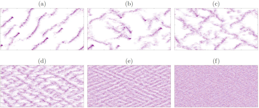
Figure 1: (a) $\mathrm{Re}=850$ ($\mathrm{Re}_{\rm b}\approx 789$): one-sided LTB regime. (b) $\mathrm{Re}=1050$ ($\mathrm{Re}_{\rm b}\approx 947$): two-sided LTB regime. (c) $\mathrm{Re}=1200$ ($\mathrm{Re}_{\rm b}\approx 1012$): strongly intermittent loose continuous network of LTBs. (d) $\mathrm{Re}=1800$ ($\mathrm{Re}_{\rm b}\approx 1237$): weakly intermittent loose banded pattern. (e) $\mathrm{Re}=3000$ ($\mathrm{Re}_{\rm b}\approx 1604$): tight banded pattern. (f) $\mathrm{Re}=4000$ ($\mathrm{Re}_{\rm b}\approx 1843$): nearly featureless state. Flow direction is from the left to right. The wall-normal velocity field on the center plane $(y=0)$ is displayed. Domain size is $500\times 250$. See Supplemental Videos SM .

Snapshots of flow patterns for typical Reynolds numbers are displayed in Fig. 1. For $\mathrm{Re}=850$ and $1050$, Fig. 1(a,b), several localized turbulent bands (LTBs) are observed, propagating at an angle about $45^{\circ}$ with the streamwise direction, each driven by a downstream active head (DAH) Tao and Xiong (2013); Xiong et al. (2015); Tsukahara and Ishida (2015); Tao et al. (2018); Teramura and Toh (2016); Kanazawa et al. (2017) located at its downstream extremity. DAHs entraining LTBs drift at a speed about 0.8 in the streamwise direction and about 0.1 in the spanwise direction. In agreement with previous studies Kanazawa et al. (2017); Tao et al. (2018), these LTBs decay below $\mathrm{Re}_{\rm g}\approx 700$. At $\mathrm{Re}=850$ (a), all LTBs go in the same direction, therefore breaking the symmetry with respect to the spanwise direction. By contrast, LTBs go in both directions at $\mathrm{Re}=1050$ (b). These states are respectively called one-sided and two-sided. As $\mathrm{Re}$ increases, LTBs joint to form a loose continuous network of oblique bands and for $\mathrm{Re}=1200$ (c) DAHs practically cease to be seen. The pattern is strongly intermittent with turbulence intensity far from being uniform along the bands. At larger values of $\mathrm{Re}$, the network narrows, $\mathrm{Re}=1800$ (d), and wide laminar voids disappear while regular patterns form, which can be understood as crisscrossed more acute ($\sim 25^{\circ}$) oblique turbulence modulations, $\mathrm{Re}=3000$ (e), similar to those obtained in circular Couette flow Prigent et al. (2003). The amplitude of this modulation then decreases and the featureless regime eventually prevails for $\mathrm{Re}\gtrsim 4000$ (f). Properties of the flow deeper inside the uniformly turbulent, developed regime achieved at even larger values of $\mathrm{Re}$ are briefly reviewed in Pope (2000). Figure 2 is a sketch of the bifurcation diagram of channel flow indicating the different regimes illustrated above and anticipating the output of the quantitative study of phenomena developing for $800\leq\mathrm{Re}\leq 1200$ to be presented below.

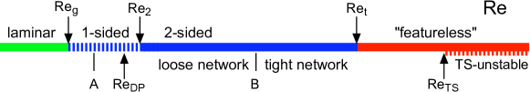
Figure 2: Bifurcation diagram for plane channel flow as obtained in our simulations. (Corresponding values of $\mathrm{Re}_{\rm b}$ between parentheses.) Laminar flow is always recovered in the long-time limit for $\mathrm{Re}<\mathrm{Re}_{\rm g}\approx 700$ ($\mathrm{Re}\equiv\mathrm{Re}_{\rm b}$ up to $\mathrm{Re}_{\rm g}$). Event A corresponds to the onset of transversal splitting at $\mathrm{Re}\sim 800$ ($\mathrm{Re}_{\rm b}\sim 795$). The extrapolated $2D$-DP threshold is found at $\mathrm{Re}_{\rm DP}\simeq 984$ ($\mathrm{Re}_{\rm b}\simeq 905$). The transition from one-sided to two-sided propagation of LTBs takes place at $\mathrm{Re}_{2}\simeq 1011$ ($\mathrm{Re}_{\rm b}\simeq 924$). Event B marks the opening of laminar gaps in the turbulent branches, sufficiently long-lived to allow the development of DAHs. It takes place at $\mathrm{Re}\approx 1200$ ($\mathrm{Re}_{\rm b}\approx 1012$). Finally, “featureless” turbulence is present for $R>\mathrm{Re}_{\rm t}\approx 3900$ ($\mathrm{Re}_{\rm b}\approx 1820$). The Tollmien–Schlichting instability threshold is at $\mathrm{Re}_{\rm TS}=5772$ (analysis refers to laminar base flow, hence identical $\mathrm{Re}_{\rm b}$).

Information from the statistics over the time-series of typical global quantities is displayed as functions of $\mathrm{Re}$ or $\mathrm{Re}_{\rm b}$ in Fig. 3 and 4. Transverse turbulent energies, $E_{y}(t)={\mathcal{V}}^{-1}\int_{\mathcal{V}}u_{y}^{2}{\rm d}{\mathcal{V}}$ and $E_{z}(t)={\mathcal{V}}^{-1}\int_{\mathcal{V}}u_{z}^{2}{\rm d}{\mathcal{V}}$, in Fig. 3(a) directly monitor the distance to the laminar base flow.

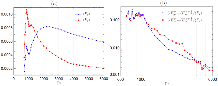
Figure 3: Means (a) and relative standard deviations (b) of the wall-normal energy $E_{y}(t)$ and spanwise energy $E_{z}(t)$.

Irregularities noted for $\mathrm{Re}<1200$ can be interpreted with the help of Fig. 1(a–c). The rapid growth of $E_{y}$ and $E_{z}$ for $\mathrm{Re}\leq 850$ is related to the increasing number of DAHs in the one-sided LTB regime. When $\mathrm{Re}>850$, the increasing fraction of LTBs with different orientations leads to a strong decrease in $E_{y}$ and $E_{z}$ until $\mathrm{Re}\approx 1000$. Next, as $\mathrm{Re}$ increases, $E_{y}$ grows again owing to an increasing turbulent fraction while $E_{z}$ slightly increases up to $\mathrm{Re}\approx 1200$ before decreasing in the band-network regime where the global flow around LTBs is inhibited. The variations of the standard deviations of fluctuations, once normalized by their respective means, are remarkably correlated, as seen in Fig. 3(b). Their rapid growth as $\mathrm{Re}$ approaches $\mathrm{Re}\approx 1000$ from above is reminiscent of the divergence of fluctuations observed for a phase transition at a threshold $\mathrm{Re}_{2}$ precisely located later. Peaks at $\mathrm{Re}=725$ and $\mathrm{Re}=800$ mark the onset of longitudinal and transversal splittings to be examined below.

Further general observations about the transitional range as a whole can be extracted from our numerical results. Using a constant body force (mean applied pressure gradient), our numerical implementation of Navier–Stokes equations produces streamwise and spanwise net flux components $U_{\rm m}$ and $W_{\rm m}$ as time-fluctuating observables governed by (11). In particular, the bulk Reynolds number $\mathrm{Re}_{\rm b}:=\frac{3}{2}\langle U_{\rm m}\rangle\mathrm{Re}$ introduced earlier is obtained from the time average of $U_{\rm m}$. Figure 4(a) displays $\langle U_{\rm m}\rangle$ as a function of $\mathrm{Re}$. Laminar flow corresponds to $U_{\rm m}^{\rm lam}=2/3$. As soon as some turbulence is present we get $\langle U_{\rm m}\rangle<U_{\rm m}^{\rm lam}$ and, for $\mathrm{Re}$ above the one-sided regime, the observed decrease nicely fits an inverse square root over a large part of the transitional range. Using results for $\mathrm{Re}\geq 1050$ we obtain $U_{\rm m}^{\rm fit}=w/\sqrt{\mathrm{Re}}$ with $w\simeq 19.5$, hence $\mathrm{Re}_{\rm b}\approx\frac{3}{2}w\sqrt{\mathrm{Re}}$. Turning to wall units, the friction velocity $U_{\tau}$ and the friction Reynolds numbers $\mathrm{Re}_{\tau}$ are obtained in our formulation as $U_{\tau}^{2}=\tau_{\rm w}=2/\mathrm{Re}$ and $\mathrm{Re}_{\tau}=\sqrt{2\mathrm{Re}}$, relation (17). This means that $\mathrm{Re}_{\tau}$ and $\mathrm{Re}_{\rm b}$ are roughly proportional as long as the flow remains textured, before entering the developed regime where $\mathrm{Re}_{\tau}$ then grows as a function of $\mathrm{Re}_{\rm b}$ at a slightly smaller rate (exponent $\simeq 0.88$ Pope (2000)). This behavior is directly reflected in the variation of the skin friction coefficient ${\rm C}_{\rm f}$ with $\mathrm{Re}_{\rm b}$ shown in Fig. 4(b). Here we have ${\rm C}_{\rm f}:=\tau_{\rm w}/\frac{1}{2}\langle U_{\rm m}\rangle^{2}=4/(\mathrm{Re}\,\langle U_{\rm m}\rangle^{2})$ (see §A). As soon as some turbulence is present, ${\rm C}_{\rm f}$ deviates from its laminar expression $9/\mathrm{Re}_{\rm b}$, remains close to it in the one-sided regime, next change to a near plateau dependence as soon as it enters in the two-sided regime, as expected from the variation of $\langle U_{\rm m}\rangle^{2}$ as $\mathrm{Re}^{-1}$ in the corresponding $\mathrm{Re}$-range. In our simulations, this plateau extends up to the transition to fully developed turbulent channel flow marked by a dotted line in Fig. 4(b), theoretically expressed as $\mathrm{Re}_{\rm b}=\frac{3}{\sqrt{2{\rm C}_{\rm f}}}\,\exp\big{(}0.41\big{(}\sqrt{2/{\rm C}_{\rm f}}-2.4\big{)}\big{)}$ Dean (1978); Pope (2000). This plateau is better defined than in earlier experiments Patel and Head (1969); Dean (1978) and simulations Xiong et al. (2015); Tsukahara et al. (2005) also shown in the picture. It indicates that, above $\mathrm{Re}_{2}$, the transition to turbulence develops at a nearly constant dissipation rate $\langle\epsilon_{\rm m}\rangle$, as stems from relation (18). In the upper transitional range $\mathrm{Re}\gtrsim 4000$, i.e. $\mathrm{Re}_{\rm b}\gtrsim 1850$, the trend suggested by our data points seems to overestimate ${\rm C}_{\rm f}$ as predicted for the fully turbulent regime Pope (2000) (dotted line). This is presumably due to a lack of resolution close to the wall at such high values of the Reynolds number. A detailed quantitative study of the transition to the “featureless” regime around $\mathrm{Re}_{\rm t}$, beyond the preliminary result in Manneville and Shimizu (2019) indicated in Figure 2, is left to future work.

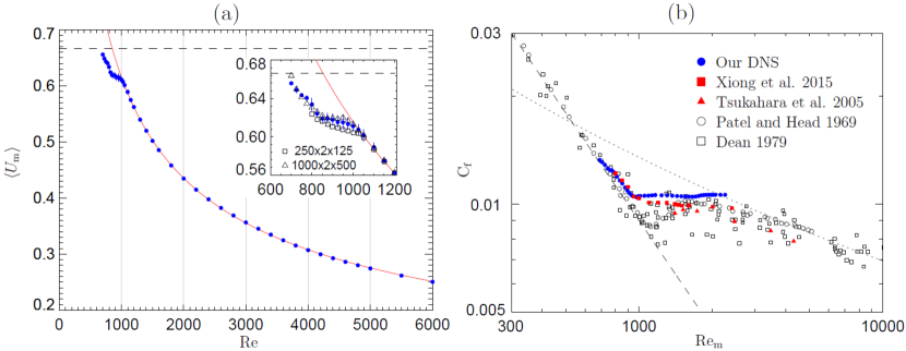
Figure 4: (a) Average of streamwise bulk velocity $\langle U_{\rm m}\rangle$ as a function of $\mathrm{Re}$; the solid line corresponds to the fit and the dashed line to laminar flow, $U_{\rm m}^{\rm lam}=2/3$. Open symbols in the inset are for the different domain sizes. (b) Skin friction coefficient ${\rm C}_{\rm f}$ as a function $\mathrm{Re}_{\rm b}$. Filled and open symbols are from DNSs (Tsukahara et al. 2005 Tsukahara et al. (2005), Xiong et al. 2015 Xiong et al. (2015)) and experiments (Patel and Head 1969 Patel and Head (1969), Dean 1979 Dean (1978)), respectively. The dashed line is for laminar flow and the dotted line for the fully turbulent regime.

III Symmetry-restoring bifurcation

Laminar–turbulent patterns below $\mathrm{Re}=1200$ were examined to better understand the symmetry-restoring bifurcation observed at increasing $\mathrm{Re}$. Processes involved in the dynamics are illustrated in Fig. 5. The local spread and decay of turbulence respectively stem from splittings and collisions of LTBs with either identical or opposite orientations. Figure 5(a) shows the nucleation of a new band by longitudinal splitting of an LTB at its tail.

(a1)    $\mathrm{Re}=725$, $t$=8000

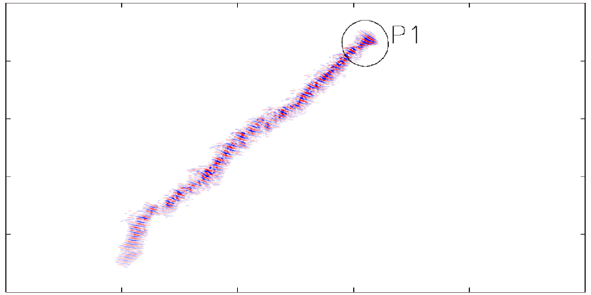
(b1)    $\mathrm{Re}=725$, $t$=59000

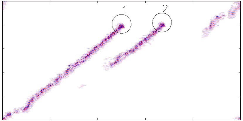
(c1)    $\mathrm{Re}=900$, $t$=53200

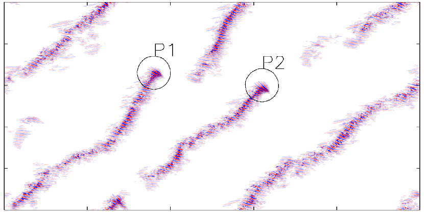
(d1)    $\mathrm{Re}=900$, $t$=136900

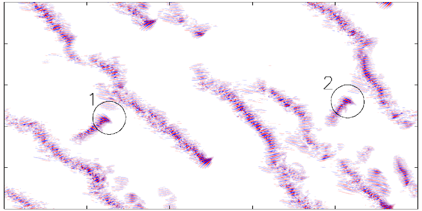
(a2)    $\mathrm{Re}=725$, $t$=9000

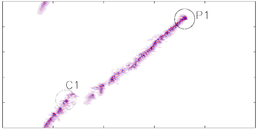
(b2)    $\mathrm{Re}=725$, $t$=62500

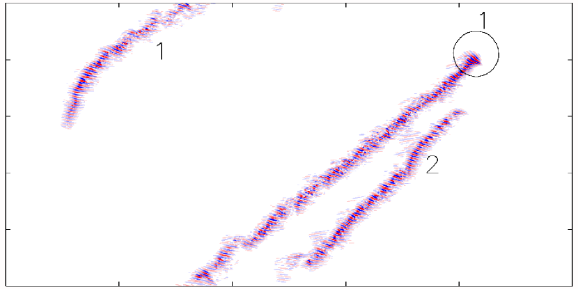
(c2)    $\mathrm{Re}=900$, $t$=53500

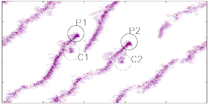
(d2)    $\mathrm{Re}=900$, $t$=137100

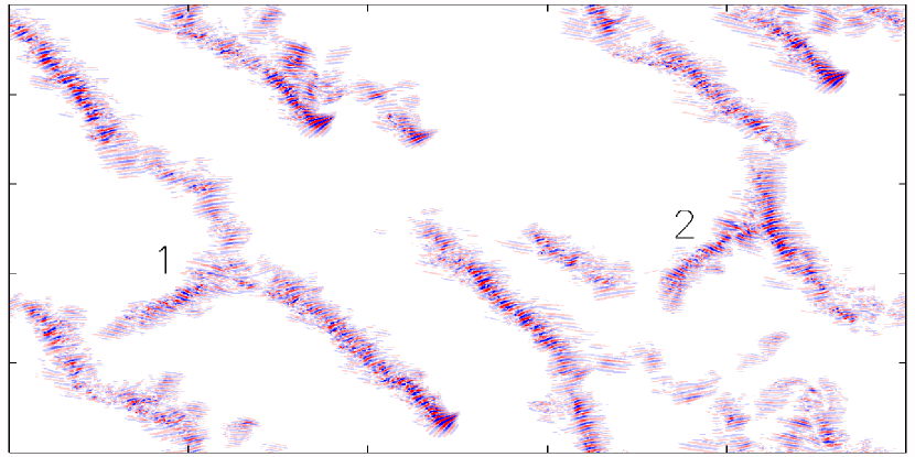
(a3)    $\mathrm{Re}=725$, $t$=10000

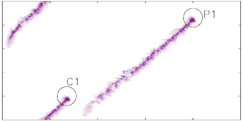
(b3)    $\mathrm{Re}=725$, $t$=63500

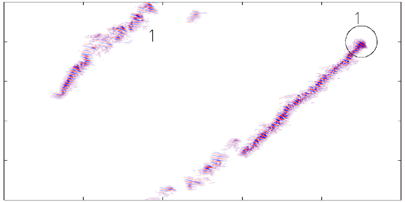
(c3)    $\mathrm{Re}=900$, $t$=53800

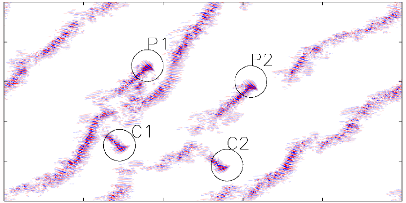
(d3)    $\mathrm{Re}=900$, $t$=137400

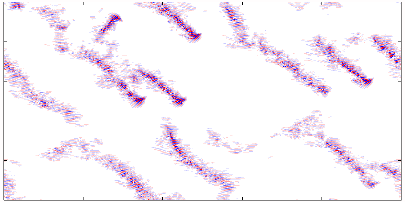
Figure 5: (a) Longitudinal splitting. (b) Longitudinal collision. (c) Transversal splitting. (d) Transversal collision. The same quantity as in Fig. 1, $u_{y}(x,0,z;t)$, is displayed in a comoving frame with velocity $({u_{x}}^{\rm(f)},{u_{z}}^{\rm(f)})=(0.8,0.1)$. Circles locate DAHs to be followed and numbers identify bands, ‘P’ and ‘C’ stand for parent and child, respectively. See also videos in SM .

The active region is downstream and the splitting takes place upstream where the turbulence level is always weaker than near the DAH, contrary to what happens for puffs in pipe flow Avila et al. (2011); Shimizu et al. (2014). When two parallel LTBs collide (longitudinal collision), following the large scale flow around them Xiong et al. (2015); Tsukahara and Ishida (2015); Tao et al. (2018), the upstream faster LTB catches the downstream LTB that disappears as in Fig. 5(b). At larger $\mathrm{Re}$, another splitting process here called transversal can take place along an LTB: A turbulent ‘bud’ appears on the side of an LTB and forms an off-aligned turbulent branch as in Fig. 5(c). Finally, when the DAH of a new-born LTB collides an LTB with a different orientation (transversal collision), the attacker most often dies in the collision, Fig. 5(d). The occurrence of transversal splitting causes the spread of turbulence to be a genuinely two-dimensional process. Transversal splitting has also been observed in plane Couette flow and considered essential to the development of laminar–turbulent patterns Manneville (2012). Although transversal splittings are observed for $\mathrm{Re}\geq 800$, one propagation direction remains dominant up to threshold $\mathrm{Re}_{2}$.

This one-sided/two-sided spanwise-symmetry restoring bifurcation can be understood using a simple prey-predator model for the densities $X_{\pm}$ of two species of LTBs, left-propagating and right-propagating:

$${\rm d}X_{+}/{\rm d}t=aX_{+}-bX_{+}^{2}+cX_{-}-dX_{+}X_{-}\,,$$ (1)

$${\rm d}X_{-}/{\rm d}t=aX_{-}-bX_{-}^{2}+cX_{+}-dX_{+}X_{-}\,.$$ (2)

By construction, these equations incorporate the built-in spanwise symmetry of the system and each term corresponds to a process in Fig. 5. Coefficient $a$ represents the longitudinal splitting rate (Fig. 5(a)). The transversal splitting rate $c$ (Fig. 5(c)), the natural control parameter, is assumed to increase with $\mathrm{Re}$ according to the observations ($c>0$ for creation of $X_{\pm}$ out of $X_{\mp}\neq 0$, hence $c\geq 0$ for $\mathrm{Re}\gtrsim 800$, event A in Fig. 2). Coefficients $b$ and $d$ account for the turbulence-level decrease by the collision between LTBs of either the same (Fig. 5(b)) or different (Fig. 5(d)) orientations. For collisions between differently oriented LTBs, the term $-dX_{+}X_{-}$ models the decay rate of one of the species $X_{\pm}$ taken as proportional to the cross-section of LTBs of the opposite kind $X_{\mp}$. Coefficient $d$, which is weakly dependent on $\mathrm{Re}$ and a function of the speed of colliding LTBs, is assumed constant, as well as $b$ parameterizing a logistic self-interaction for predation among LTBs with the same orientation, i.e. $-bX_{\pm}^{2}$. A reduced cross-section and a very small relative velocity between LTBs of the same kind suggest $b\ll d$. By contrast with works elaborating on reaction-diffusion models devised to account for local interactions in transitional flows Barkley (2016); Shih et al. (2016), our approach is Landau-like and deals with global observables minimally coupled by purely phenomenological coefficients.

The analysis of the model is straightforward when considering the total amount of turbulence $S=X_{+}+X_{-}$ and the degree of asymmetry $A=X_{+}-X_{-}$ as working variables. The equations for these variables become:

$$\frac{{\rm d}S}{{\rm d}t}=(a+c)S-\mbox{$\frac{1}{2}$}(b+d)S^{2}-\mbox{$\frac{1}{2}$}(b-d)A^{2}\,,$$ (3)

$$\frac{{\rm d}A}{{\rm d}t}=(a-c)A-bSA\,.$$ (4)

The two-sided regime labeled “$**$” corresponds to $A=0$, while $A\neq 0$ implies the dominance of one propagation direction. “$A_{**}=0$” solves (4) in all circumstances. Using (3), the symmetrical fixed point is then given by:

$$S_{**}=\frac{2(a+c)}{b+d}\,,\qquad A_{**}=0.$$ (5)

This fixed point has eigenvalues ($s_{S},s_{A}$) with $s_{S}=-(a+c)<0$ and $s_{A}=[a(d-b)-c(d+3b)]/(b+d)$. The symmetric solution is then stable as long as $s_{A}<0$; hence, $c>c_{\rm c}=a(d-b)/(d+3b)$ when $b<d$ as assumed from the observations. The two-sided regime is then stable for large $\mathrm{Re}$ and becomes unstable below a threshold corresponding to $c_{\rm c}$.

The one-sided regime labeled “$*$” corresponds to $A\neq 0$ at steady state (fixed point); hence, from (4) and next from (3):

$$S_{*}=\frac{a-c}{b}\,,\quad{A_{*}}^{2}=\frac{(a-c)(d+3b)(c_{\rm c}-c)}{b^{2}(d-b)}\,.$$ (6)

This analysis shows that the system experiences a standard super-critical pitchfork bifurcation toward asymmetry by decreasing $c$. At $c=c_{\rm c}$ as previously defined, $(S_{**},A_{**})$ becomes unstable and is replaced by $(S_{*},\pm A_{*})$, which is stable for $c<c_{\rm c}$ as expected. Figure 6(a) displays the bifurcation diagram of model (3,4) with splitting rate $c$ taken as the control parameter, and $a=10^{-4}$, $d=10$, $b=d/10$. The thick line represents the total turbulence amount $S$ given by $S_{*}=(a-c)/b$ below $c_{\rm c}$ and $S_{**}=2(a+c)/(b+d)$ above. Thin lines correspond to $X_{\pm}$. Dashed lines correspond to the unstable solutions (the dashed branch for $c>a$ is furthermore irrelevant to the present problem since it leads to negative values of $X_{-}$).

Experimental support to the model is displayed in the boxed region in Fig. 6(b). The total transverse perturbation energy $E_{y}+E_{z}=E_{2D}$ is taken as a proxy for $S$. The mean spanwise velocity component $W_{\rm m}={\mathcal{V}}^{-1}\int_{\mathcal{V}}u_{z}{\mathrm{d}}{\mathcal{V}}$ is interpreted as an instantaneous measure of the degree of asymmetry $A$ because it cancels out statistically when symmetry is restored at high $\mathrm{Re}$, i.e. $\langle W_{\rm m}\rangle=0$, where $\langle\cdot\rangle$ represents time average. Notice that the standard deviation of $E_{2D}$ is multiplied by 6 and both $\langle W_{\rm m}\rangle$ and its standard deviation are divided by 4 so that variations of the observables can be more easily compared. As long as transversal splitting is negligible, $\langle E_{2D}\rangle$ and $\langle W_{\rm m}\rangle$ increase with the mean length of LTBs. The two orientations correspond to $\langle W_{\rm m}\rangle$ with opposite signs. Periodic spanwise boundary conditions leave open the possibility of having $W_{\rm m}\neq 0$ as a result of symmetry breaking. The case of an experimental system with solid lateral boundaries forbidding such a net transverse flux is considered later in §V. In Figure 6(b) we only display $|\langle W_{\rm m}\rangle|$ since at steady state, depending on the orientation of the LTBs, $\pm|\langle W_{\rm m}\rangle|$ are equally possible. Both $\langle E_{2D}\rangle$ and $|\langle W_{\rm m}\rangle|$ reach their maximum values for $\mathrm{Re}\approx 850$, which can be understood as when transversal splitting –not observed below $\mathrm{Re}=800$– becomes significant. For $\mathrm{Re}>850$, our two observables follow the trend suggested by the model: $\langle E_{2D}\rangle$ decreases roughly linearly as $\mathrm{Re}$ increases up to $\mathrm{Re}\approx 1000$ and slowly grows beyond, in agreement with equations (5, 6). Likewise, $|\langle W_{\rm m}\rangle|$ decreases rapidly to zero, similar to $A_{*}$, as indicated by the fact that the standard deviation becomes larger than the mean, at $\mathrm{Re}\approx 1000$. For larger $\mathrm{Re}$ outside the box, the system enters a developed two-sided regime where the model, designed to account for the one-sided/two-sided bifurcation, becomes insufficient. Inside the box, this oversimplified formulation well captures the phenomenology of the transition at a qualitative level.

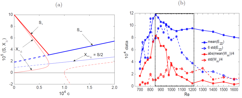
Figure 6: Transition from one-sided to two-sided flow. (a) Model. (b) Numerical simulation.

The transition is then understood by assuming that parameter $c$ measuring the transversal splitting rate increases with $\mathrm{Re}$. The analysis above shows that $c_{\rm c}\simeq a$ assuming that $b\ll d$, as stems from our observations. Furthermore, in the range $850\leq\mathrm{Re}\leq 1200$, the variations of $S$ and $A$ around $c_{\rm c}$ are consistent with those of the turbulent energy and the spanwise mean velocity, respectively. In fact, the deviation of $\langle U_{\rm m}\rangle$ away from its behavior in the two-sided regime fitted as $U_{\rm m}^{\rm fit}=w/\sqrt{\mathrm{Re}}$ in Fig. 4(a) is a proxy for the change of total amount of turbulence at the one-sided/two-sided bifurcation. As displayed in Fig. 7, this variation is linear close to the bifurcation point $\mathrm{Re}_{2}\simeq 1011$, in agreement with the predictions of the model. As can be seen in the inset of Fig. 4(a) and in Fig. 7, the current domain size is appropriate to obtain this threshold.

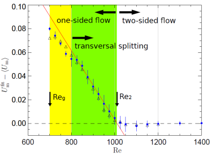
Figure 7: Departure of observed streamwise mean flow $\langle U_{\rm m}\rangle$ from the value predicted by the law $U_{\rm m}^{\rm fit}=19.47/\sqrt{\mathrm{Re}}$, solid line in Fig. 4(a). Fitting the data against a straight line for $850\leq\mathrm{Re}\leq 1000$ yields $\mathrm{Re}_{2}\simeq 1011$. Triangles are for the larger domain $1000\times 2\times 500$.

IV Behavior above $\mathrm{Re}_{2}$

Beyond $\mathrm{Re}_{2}$ and up to entrance in the tight-banded pattern regime, Fig. 1(e), channel flow exhibits a spatiotemporal intermittent behavior, Fig. 1(c,d), strongly reminiscent of DP above the threshold. The work of Sano and Tamai Sano and Tamai (2016) focusing on the critical properties of turbulence decay in a DP context Henkel et al. (2008) naturally suggests one to study this Reynolds number range in terms of turbulent fraction $F_{\rm t}$. This in turn relies on the identification of appropriate laminar and turbulent local states, based on observables that vary sufficiently sharply in space to define the respective domains properly, allowing a precise measurement of their relative occupancy fractions. Figure 8 displays four possible candidates, the three velocity components in the mid-gap plane $y=0$, and the mean transverse perturbation energy $E_{2D}(x,z;t)=\frac{1}{2}\int_{-1}^{1}(u_{y}^{2}+u_{z}^{2})\,{\rm d}y$ around an LTB at $\mathrm{Re}=700$.

$u_{x}(y=0)$

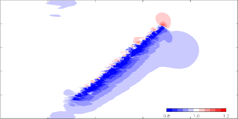
$u_{z}(y=0)$

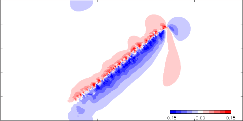
$u_{y}(y=0)$

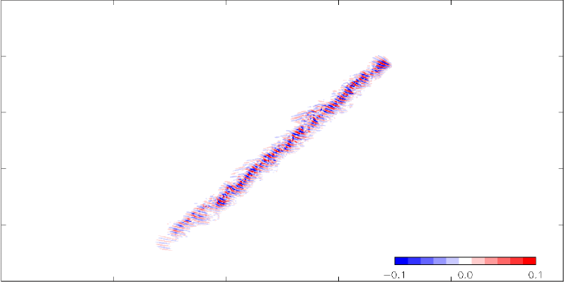
$\langle u_{y}^{2}+u_{z}^{2}\rangle_{y}$

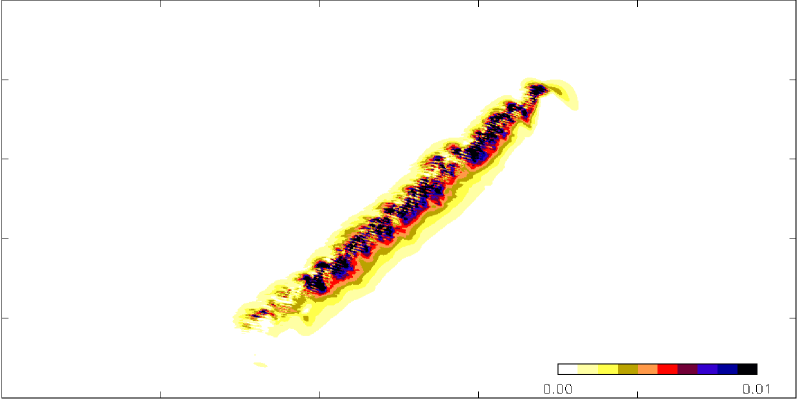
Figure 8: Possible candidates for the determination of the turbulent fraction illustrated by ${2D}$-images of the same localized turbulent band at $\mathrm{Re}=700$. The flow is from left to right and the downstream active head is in the upper right corner in each panel. Domain size is $500\times 250$.

In-plane components $u_{x}$ and $u_{z}$ display a large-scale, slowly decaying, structure around the LTB. By contrast, $u_{y}$ sharply discriminates non-laminar flow regions. $E_{2D}$ is slightly less close-fitting due to the limited contribution of the component $u_{z}$. Accordingly, the absolute value of the wall-normal velocity on the mid-plane $|u_{y}(x,0,z)|$ will be used to evaluate $F_{\rm t}$. However, inside LTBs, $u_{y}$ displays small-scale oscillations associated with the presence of streamwise vortices, which produces narrow regions with $|u_{y}(x,0,z)|\approx 0$ that must not be counted as laminar. Accordingly, the field $|u_{y}(x,0,z)|$ has to be smoothed beforehand, here by simple box-averaging over cells of size $w\times w$, and next thresholded using the “moment-preserving” procedure Tsai (1985), as explained in Appendix B.

The variation of $F_{\rm t}$ as a function of $\mathrm{Re}$ is displayed in Fig. 9(a) for $700\leq\mathrm{Re}\leq 3000$ and for $w$ varying between 0 (no filtering) and $40\delta$.

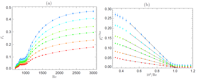
Figure 9: $F_{t}$ for different $w$. From the bottom to the top: $w=0$ (no filtering, red), $4\delta$, $8\delta$, $12\delta$, $20\delta$, and $40\delta$ (blue). (a) $F_{\rm t}$ as a function of $\mathrm{Re}$. (b) $F_{t}^{1/\beta_{\rm DP}}$ as a function of $1/\mathrm{Re}$ with $\beta_{\rm DP}=0.583$.

For all values of $w$, similar variations are observed and one readily identifies the different stages illustrated in Fig. 1: one-sided growth for Re $\leq\mathrm{Re}_{2}\simeq 1011$, with a clear change of regime for $\mathrm{Re}\sim 850$ as transversal splitting sets in, before a rapid increase akin to a power-law growth as $\mathrm{Re}$ increases in the symmetry-restored regimes (Fig. 1(b)-(d)) up to the tight banded pattern regime (Fig. 1(e)).

The consistent square-root-like behavior is reminiscent of the growth of the order parameter of DP beyond threshold. In line with the idea that the critical properties of the stochastic DP process are relevant for channel flow, as put forward by Sano & Tamai, we first test the plausibility of exponent $\beta_{\rm DP}\simeq 0.583$ to describe the variation of the turbulent fraction with the relative distance to threshold. Figure 9(b) therefore displays $F_{\rm t}^{1/\beta_{\rm DP}}$ as a function of $1/\mathrm{Re}$. The linear behavior of the plots for different values of $w$, systematically extrapolating to zero for around $\mathrm{Re}\approx 1000$ ($1000/\mathrm{Re}\approx 1)$ therefore strongly supports the expected behavior of $F_{\rm t}$ as if it were produced by a $2D$-DP process. From the least-square fits, the straight lines in Fig. 9(b), it is seen that some filtering is needed to eliminate spurious small scale oscillations of $u_{y}(x,0,z)$ since raw data ($w=0$, red data points) does not behave so satisfactorily. On the other hand, strong filtering ($w\geq 20$) leads to a reduction of the range where a good linear fit is obtained ($1050\leq\mathrm{Re}\leq 2400$ for $w\leq 12\delta$, and $1050\leq\mathrm{Re}\leq 2000$ for $w=20\delta$ and $40\delta$). To further develop the quantitative analysis we choose the best compromise which seems to be $w=12\delta$, i.e. the largest filtering possible in the widest $\mathrm{Re}$ interval with the expected property.

In these conditions, a direct fitting over the interval $1050\leq\mathrm{Re}\leq 2400$ has been attempted against the function $F_{\rm t}=B\left(1-\mathrm{Re}_{\rm DP}/\mathrm{Re}\right)^{\beta}$ with $B$, $\mathrm{Re}_{\rm DP}$ and $\beta$ as fitting parameters. We proceeded to a least-square minimization of the error ${\rm Err}^{2}=$
$\frac{1}{N}\sum_{n=1}^{N}\left({F_{\rm t}}_{n}-B\big{(}1-\mathrm{Re}_{\rm DP}/\mathrm{Re}_{n}\right)^{\beta}\big{)}^{2}$ where $N$ is the number of values $\mathrm{Re}_{n}$ of $\mathrm{Re}$ entering the fit, and ${F_{\rm t}}_{n}$ the corresponding measured mean turbulent fraction. Figure 10(a) displays the minimum error as a function of $\beta$, pointing to $\beta\approx 0.58$, while panels (b) and (c) display similar results for $B\approx 0.45$ and $\mathrm{Re}_{\rm DP}\approx 984$ as best fitting values, respectively. Following this approach, the estimate for $\beta$ turns out to be close to the theoretical value $\beta_{\rm DP}=0.583$ that served as initial guess in Fig. 9(b). The error curves in each case however indicate that the optima are not sharply defined. Unfortunately, these estimates cannot be improved mainly because the critical point cannot be approached sufficiently closely. This also justifies that we did not try to adjust the other critical parameters related to space-time correlations since they are discriminating solely in an arbitrarily close neighborhood of $\mathrm{Re}_{\rm DP}$.

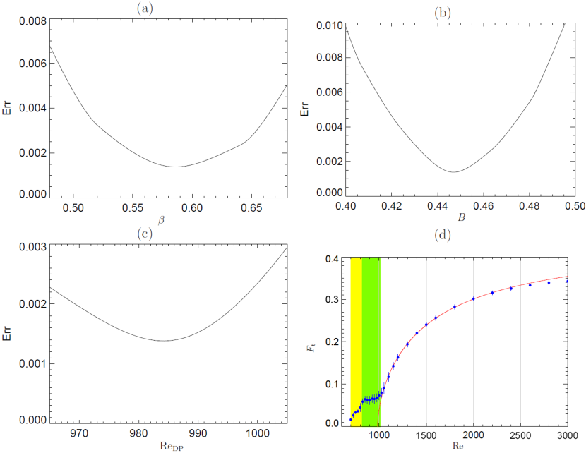
Figure 10: (a–c) Minimum of ${\rm Err}$ as a function of the different fit parameters for $F_{\rm t}$ with $w=12\delta$ and control parameter $1/\mathrm{Re}$. (a) Exponent $\beta$. (b) Amplitude $B$. (c) Threshold $\mathrm{Re}_{\rm DP}$. In these panels, the error is displayed as a function of one fitting parameter, the two other being supposed fixed at their optimal value. (d) Turbulent fraction $F_{\rm t}$ as a function of $\mathrm{Re}$ and its fit against the theoretical expression given in §IV

Our results, used to draw the fitting line in Fig. 10(d), therefore point toward a plausible universal DP behavior for large enough turbulent fraction, a behavior inevitably truncated before criticality by a crossover to a different decay regime as $\mathrm{Re}$ decreases. As a matter of fact, the turbulent fraction becomes so small that laminar gaps open along oblique arms of the fluctuating laminar-turbulent network, which produces the development of DAHs –original to channel flow– so that the DP regime is superseded by the LTB-dominated regime and, as $\mathrm{Re}$ decreases even more, to the symmetry-breaking bifurcation below which turbulence decay takes up a novel turn.

V Discussion and concluding remarks

Apart from a few illustrations of the laminar-turbulent patterning in the upper transitional range of channel flow in Fig. 1(e,f), our results all relate to its lower part featuring the decay to laminar flow where a DP scenario with universal properties expected for two-dimensional systems has been put forward Sano and Tamai (2016), while sustained LTBs have been observed at values of $\mathrm{Re}$ lower than the measured DP critical point Tao and Xiong (2013); Xiong et al. (2015); Tsukahara and Ishida (2015); Kanazawa et al. (2017); Tao et al. (2018); Hof (2016); Paranjape et al. (2017). The first result comes in support of a theoretical conjecture by Pomeau Pomeau (1986) based on the recognition that the flow can be locally in one of the two possible states, turbulent or laminar. Furthermore, in the transitional range, developing turbulence presents itself as a contamination of the laminar state, locally linearly stable and therefore absorbing, by a highly fluctuating, unstable, chaotic active state. This framework is directly derived from a statistical-physics approach where the key concept is the thermodynamic limit of infinitely wide systems at statistically steady state (here non-equilibrium steady state). Though experiments and simulations are performed in domains and for durations somewhat far from the thermodynamic-limit conditions (with Chantry et al. (2017) as a possible exception), the question of what we may infer on general grounds from our results is relevant.

Let us first notice that comparisons with laboratory experiments and computer simulations are made difficult owing to the several possibilities chosen to drive the flow, either generated by a fixed pressure gradient (or given average friction at the walls) or a constant mean streamwise flow rate. Though it is generally admitted that the results should be statistically identical at the thermodynamic limit, quantitative correspondence between different works is not easy to establish, and first of all with respect to how $\mathrm{Re}$ is defined owing to what is controlled and what is measured. Here we fix the mean pressure gradient (fixed bulk force $f$) and use the computed centerline velocity of the corresponding laminar flow $U$ as speed unit, while the half-distance $h$ between the plates is taken as length unit and $h/U$ as time unit. The definition of $\mathrm{Re}=Uh/\nu$ follows. If wall units are preferred, e.g. in Tsukahara et al. (2005), one gets $\mathrm{Re}_{\tau}=\sqrt{2\mathrm{Re}}$ as derived in §A. In the laminar regime the mean flow rate is $U_{\rm m}=\frac{2}{3}U$ and the Reynolds number made out of it: $\mathrm{Re}_{\rm m}=U_{\rm m}h/\nu=\frac{2}{3}\mathrm{Re}$ is frequently used. However, when the flow is not fully laminar, the measured mean flow rate $\langle U_{\rm m}\rangle$ decreases below its nominal value $2/3$ (Fig. 7). Accordingly, the Reynolds number constructed using $\langle U_{\rm m}\rangle$ is not a control parameter but an observable that has to be determined by averaging $u_{x}$ over space and time. This lead us to define $\mathrm{Re}_{\rm b}=\frac{3}{2}\langle\mathrm{Re}_{\rm m}\rangle=\frac{3}{2}\langle U_{\rm m}\rangle h/\nu$. With this definition, when the flow is fully laminar, $\mathrm{Re}_{\rm b}\equiv\mathrm{Re}$ and, accordingly, the linear instability threshold is $\mathrm{Re}_{\rm TS}=5772$ Orszag (1971). Willing to keep $\langle U_{\rm m}\rangle$ strictly constant, as done in some numerical experiments and only approximately achieved in the laboratory, is therefore a different experiment in which the applied pressure gradient is unknown and fluctuating. All in all, our results in Fig. 1 are consistent with those found in the literature when expressed in terms of $\mathrm{Re}_{\rm b}$, especially those in Tsukahara et al. (2005); Tao et al. (2018), or even in Tuckerman et al. (2014); NB .

Our main contention is that the previously mentioned conflicting experimental observations about DP universality and the existence of LTBs can be reconciled provided that it is recognized that the DP scenario cannot be followed down to its critical point. We have shown that, when the turbulent fraction is small enough, processes develop which are not present in other systems where DP-universality is observed: As $\mathrm{Re}$ is slowly decreased, the flow evolves from the weakly intermittent loose banded pattern regime, Fig. 1(d), to the strongly intermittent continuous network regime, Fig. 1(c). Further decreasing $\mathrm{Re}$ induces the opening of laminar gaps along the turbulent branches, here called splittings, and the formation of LTBs terminated by DAHs constitutive of the two-sided LTB regime, Fig. 1(b). At first the intermittent expansion/recession of turbulence is two-dimensional in the plane of the flow owing to comparable rates for transversal and longitudinal splittings, but the rate of transversal splittings decreases with $\mathrm{Re}$ faster than that of longitudinal splittings, which implies a change to one-sided LTB propagation, i.e. a symmetry breaking due to a deficit of regeneration of one of the two LTB species at a local scale. In the long term, the rate difference indeed brings about a global dominance of one orientation over the other and a mostly one-dimensional expansion/recession of turbulence. In this respect the cases of Waleffe flow Chantry et al. (2017) and plane Couette flow Shimizu et al. (2017) appear different. In these two cases, laminar gaps also open through splittings, longitudinal and transversal, along the turbulent segments forming the fluctuating laminar-turbulent network but the upstream-downstream distinction does not make sense. Close to $\mathrm{Re}_{\rm g}$, the turbulent patches accordingly take the form of fluctuating short oblique straight segments, v-shaped, or x-shaped spots (Chantry et al., 2017, Fig. 2) with dynamics profoundly different from that of LTBs equipped with DAHs. As a result the turbulent fraction can then decrease indefinitely according to $2D$-DP universality, down to $\mathrm{Re}_{\rm DP}$ that is reached before any symmetry-breaking bifurcation has a chance to take place, presumably because the longitudinal and transversal splitting rates remain comparable as $\mathrm{Re}$ decreases. By contrast, specificities of channel flow prevent the observation of a complete $2D$-DP scenario and the origin of this imperfection is fully characterized as the result of an unavoidable symmetry-breaking bifurcation when the turbulent fraction becomes small enough, before the expected $\mathrm{Re}_{\rm DP}$ is reached.

We now focus the discussion on two main points: the variation of the turbulent fraction in the range $1050\leq\mathrm{Re}\leq 2400$ in connection with the DP scenario above the symmetry-breaking bifurcation, and the non-zero mean transverse flow in the symmetry broken regime, $\mathrm{Re}\leq\mathrm{Re}_{2}$, its observability at the thermodynamic limit or, at the opposite, in laterally bounded finite-width channels.

For the conceptual reasons already evoked, DP is relevant as a process in the lowest transitional range. In its simplest formulation used to typify the universality class, a single contamination probability is needed to control the transition but the nature of physical mechanisms involved and their dependence on the Reynolds number are not known. The expectation for universality rests on the Janssen–Grassberger conjecture Henkel et al. (2008) stipulating in particular that the absorbing state is unique, the interactions are local, and that there are no weird parasitic effects such as quenched disorder, which is implicitly assumed if Pomeau’s educated guess is valid. Strictly speaking, the question whether the decay of turbulence in channel flow follows $2D$-DP universality is void since the critical regime – the immediate neighborhood of the threshold – cannot be entered, but results presented in §IV suggest a positive answer if we accept to loosen this restriction (Fig. 10).

This argument however hides a difficulty since, as already mentioned, the relation between the chosen external control parameter and the internal control parameter, the effective contamination probability generated by stochastic processes at the scale of a few MFUs, is not known. On general grounds, the critical behavior is not sensitive to the choice of the external control parameter in an asymptotically close vicinity of the critical point while departures from universality become conspicuous at variable distances from the threshold depending on that choice. In the previously reported cases, the variation of the turbulent fraction as a function of the Reynolds number deviates from the expected power law dependence beyond a relative distance $\epsilon$ to the critical point $\sim 10^{-2}$ for quasi-$1D$ plane Couette flow (Lemoult et al., 2016, Fig. 2), or $\sim 10^{-3}$ for quasi-$2D$ Waleffe flow (Chantry et al., 2017, Fig. 4). For channel flow, the universal behavior of the turbulent fraction is reported for $\epsilon\lesssim 0.1$ in (Sano and Tamai, 2016, Fig. 3), but the experimental conditions do not permit access to the LTB regime. By contrast, taking advantage of a streamwise periodically continued domain, our approach leaves sufficient time for turbulent patches to rearrange into LTBs, which truncates the DP behavior above threshold NRm . Our most striking finding is that, characterizing the flow by its natural control parameter $\mathrm{Re}$, the turbulent fraction then varies in accordance with universality over a surprisingly wide interval from below $\mathrm{Re}\approx 2400$ nearly down to $\mathrm{Re}_{2}$ where the dynamics becomes controlled by LTBs. When expressed in terms of $\epsilon=1-\mathrm{Re}_{\rm DP}/\mathrm{Re}$ with $\mathrm{Re}_{\rm DP}=984$ as the extrapolated threshold, this range extends over $0.07\lesssim\epsilon\lesssim 0.6$ (Figs. 9(b) and 10(d)). At this point, it is fair to add that other possibilities for the external control, namely using $\mathrm{Re}_{\tau}$ or $\mathrm{Re}_{\rm b}$ in principle equivalent in the neighborhood of the threshold, perform badly at some distance above threshold, not even permitting to detect a neat power-law variation over such a wide interval. The physical meaning of $\mathrm{Re}_{\tau}$ or $\mathrm{Re}_{\rm b}$ implies an averaging over the flow in a strongly inhomogeneous spatiotemporally intermittent state, which might explain that the probabilities issued from the dynamics at the MFU scale are less straightforwardly parameterized using them than using $\mathrm{Re}$ (or $1/\mathrm{Re}$).

Let us now turn to the symmetry breaking observed at decreasing $\mathrm{Re}$ and studied in §III. Elementary events involved in the dynamics of LTBs were described in detail (Fig. 5). A satisfactory simple phenomenological model was developed then in the spirit of Landau theory to account for the bifurcation at a qualitative and semi-quantitative level. Extrapolating our results in a finite size domain with periodic boundary conditions to a laterally unbounded system (thermodynamic limit), when transversal splitting is negligible ($\mathrm{Re}\lesssim 800$) one-sided propagation is expected because for $\mathrm{Re}$ low enough, any transversal collision destroys one of the colliders (Fig. 5(d)) and, as seen in the movies at low $\mathrm{Re}$ SM , the transient evolution of sparse turbulence follows a majority rule. At short times, a patchwork of domains with one or the other dominant orientation forms, with transversal collisions concentrated along the domain boundaries. At longer times, a ripening process develop during which domains compete with each other, locally applying the majority rule so that, in the very long time limit at very low LTB density, one can figure out an asymptotic steady state which is mostly uniformly oriented. Residual LTBs are then moving nearly at the same speed, along the same direction, and interact only through longitudinal splittings/collisions (Fig. 5(a,b)) maintaining a state free of transversal collisions. Such a regime is expected to persist down to $\mathrm{Re}_{\rm g}$ below which it decays, much like in pipe flow Avila et al. (2011), due to the predominance of longitudinal destructive collisions over expanding turbulence through splittings to be discussed in a future publication Shimizu and Manneville (2019).

The difficulty with this picture is that, on general grounds, such a symmetry breaking is associated to a large scale flow with a transverse component corresponding to a net, fluctuating, spanwise mean flux with non-zero average $\langle W_{\rm m}\rangle$. In systems with periodic spanwise boundary conditions, symmetries do not forbid the existence of such a flow. Close to the bifurcation point, for $\mathrm{Re}<\mathrm{Re}_{2}$ when transversal splitting plays a significant role, the patchwork alluded to above can reach a statistically steady state with $\langle W_{\rm m}\rangle\neq 0$ but reduced by compensations between patches of different orientations, whereas for $\mathrm{Re}>\mathrm{Re}_{2}$ one gets $\langle W_{\rm m}\rangle\approx 0$ with substantial fluctuations, see Fig. 6(b). These are the characteristics of an order parameter apt to quantify the symmetry-breaking bifurcation. From the observations reported in the previous paragraph, these properties are expected to hold also as $t$ goes to infinity in a spanwise unbounded system (thermodynamic limit).

In finite-width channels with impervious lateral walls, any net spanwise mean flow $W_{\rm m}$ is not permitted. In laboratory experiments where this condition applies, the one-sided regime has been observed Hof (2016); Paranjape et al. (2017) but, in contrast with our simulations where LTBs drift obliquely, after an initial transient stage during which the flow equilibrates, they are advected strictly along the streamwise direction. This means that an additional spanwise pressure wave accompanies the passing of an LTB, producing a spanwise mean flow component able to deviate it, thus compensating for the $W_{\rm m}$ that it would naturally generate. Rigid lateral walls are obviously able to withstand such pressure fluctuations as LTBs pass by. Only simulations specially designed to implement the corresponding no-slip lateral boundary conditions, e.g. with spanwise Chebyshev polynomials Takeishi et al. (2015), would permit a detailed account of the LTB propagation in the one-sided regime. However, while keeping spanwise periodic boundary conditions, one can think of correcting our governing equations for an additional spanwise fluctuating bulk force generating a mean transverse flow sufficient to compensate the drift of LTBs and statistically maintain a strictly streamwise propagation. Such a work remains to be done but could give hints on the one-sided regime in realistic experimental conditions, owing to the obvious robustness of LTBs.

Two complementary studies are in progress, above and below the range of Reynolds numbers considered in this work: one is dedicated to the decay of the one-sided regime in a domain $1000\times 2\times 500$ or larger Shimizu and Manneville (2019) and the other is focussed on the onset of the laminar-turbulent patterning via standard Fourier analysis rather than turbulent fraction determination (Manneville and Shimizu, 2019, see Fig. 4 for preliminary results).

By way of conclusion, the introduction of concepts and methods of statistical physics, and notably directed percolation, have put stress on universal features of the transition from/to turbulence in wall-bounded shear flows. All over the spatiotemporally intermittent regimes along the transitional range of channel flow, laminar-turbulent coexistence with a high level of stochasticity legitimates Pomeau’s views Pomeau (1986) about the decay of turbulence at $\mathrm{Re}_{\rm g}$ as a process in the $2D$-DP universality class. We have shown that this claim is however only partly fulfilled because a specific phenomenon comes and renders the full scenario imperfect: spanwise symmetry is broken due to a sensitive balance between local processes (longitudinal vs. transversal splittings) with rates depending on $\mathrm{Re}$ in different ways, ending with recession/expansion of turbulence becoming mostly one-dimensional before $2D$-DP criticality has a chance to be observed. In turn this symmetry breaking is an event that could be well understood within the standard framework of dynamical systems and bifurcation theory, bringing an original perspective to the debated issue of universality vs. specificity in the transition to turbulence of wall-bounded flows.

Appendix A System and numerical procedures

We consider the flow between two parallel walls driven by a time-independent body force, usually called channel flow or plane Poiseuille flow. The equations governing the velocity field $\bm{u}$ are as follows:

$$\mbox{(a)}\quad\nabla\cdot\bm{u}=0\,,\hskip 30.00005pt\mbox{(b)}\quad\frac{\partial\bm{u}}{\partial t}+(\bm{u}\cdot\nabla)\bm{u}=-\frac{1}{\rho}\nabla p+\nu\Delta\bm{u}+f\hat{\bm{e}}_{x}\,,$$ (7)

where $\rho={\rm Const.}$ is the density, $\nu$ the kinematic viscosity, and $f$ the body force specific density. The unit vector in the streamwise direction $x$ is denoted as $\hat{\bm{e}}_{x}$. The $y$- and $z$-axes are along the wall-normal and spanwise directions, respectively. All fields are assumed in-plane periodic and the velocity fulfills the usual no-slip boundary conditions at the walls.

The center-plane velocity of the corresponding laminar flow is $U=fh^{2}/2\nu$, where $2h$ is the distance between the walls. The Reynolds number is defined as $\mathrm{Re}=Uh/\nu=fh^{3}/2\nu^{2}$. Using $h$ and $U$ as distance and velocity units, and $h/U$ as the time unit, all variables below are assumed dimensionless without a notational change, the equations governing the velocity field $\bm{u}(x,y,z,t)$ are as follows:

$$\mbox{(a)}\quad\nabla\cdot\bm{u}=0\,,\hskip 30.00005pt\mbox{(b)}\quad\frac{\partial\bm{u}}{\partial t}+(\bm{u}\cdot\nabla)\bm{u}=-\nabla p+\frac{1}{\mathrm{Re}}\Delta\bm{u}+\frac{2}{\mathrm{Re}}\hat{\bm{e}}_{x}.$$ (8)

In practice, these equations are rewritten for the wall-normal velocity component $u_{y}(x,y,z,t)$ and the wall-normal vorticity $\omega_{y}(x,y,z,t)=(\nabla\times{\bm{u}})_{y}$ obtained by applying $\nabla\times$ and $\nabla\times\nabla\times$ to (8b) and keeping its $y$ component Schmid and Henningson (2012):

$$\mbox{(a)}\quad\frac{\partial\omega_{y}}{\partial t}=(\nabla\times{\bm{N}})_{y}+\frac{1}{\mathrm{Re}}\Delta\omega_{y}\,,\hskip 30.00005pt\mbox{(b)}\quad\frac{\partial\Delta u_{y}}{\partial t}=-(\nabla\times\nabla\times{\bm{N}})_{y}+\frac{1}{\mathrm{Re}}\Delta\Delta u_{y}\,,$$ (9)

where ${\bm{N}}=\bm{u}\times\bm{\omega}$.

The full solution requires additional equations for in-plane averaged velocity fields. We define the auxiliary fields $\phi_{x}(y,t)$ and $\phi_{z}(y,t)$ as $\partial_{y}\phi_{x}=\langle u_{x}\rangle_{xz}$ and $\partial_{y}\phi_{z}=\langle u_{z}\rangle_{xz}$, where $\langle g\rangle_{xz}$ denotes in-plane averaging of field $g$, namely $(L_{x}L_{z})^{-1}\int_{0}^{L_{z}}\int_{0}^{L_{x}}g\,{\rm d}x\,{\rm d}z$. By averaging the $z$ and $x$ components of the vorticity equation $\nabla\times$ (8b) we obtain:

$$\mbox{(a)}\quad\frac{\partial}{\partial t}\frac{\partial^{2}\phi_{x}}{\partial y^{2}}=\frac{\partial\langle{\bm{N}}_{x}\rangle_{xz}}{\partial y}+\frac{1}{\mathrm{Re}}\frac{\partial^{4}\phi_{x}}{\partial y^{4}}\,,\hskip 30.00005pt\mbox{(b)}\quad\frac{\partial}{\partial t}\frac{\partial^{2}\phi_{z}}{\partial y^{2}}=\frac{\partial\langle{\bm{N}}_{z}\rangle_{xz}}{\partial y}+\frac{1}{\mathrm{Re}}\frac{\partial^{4}\phi_{z}}{\partial y^{4}}\,.$$ (10)

Fields $\phi_{x}$ and $\phi_{z}$ are defined up to arbitrary functions of time that can be fixed as follows: The streamwise bulk velocity is given by the difference between the boundary values of $\phi_{x}$ at $y=\pm 1$, $U_{\rm m}=\frac{1}{2}\int_{-1}^{+1}\langle u_{x}\rangle_{xz}{\rm d}y=\frac{1}{2}[\phi_{x}(y,t)]_{y=-1}^{y=+1}$. The arbitrariness in the definition of $\phi_{x}$ can then be lifted by choosing $\phi_{x}(+1,t)=U_{\rm m}(t)$; hence, $\phi_{x}(-1,t)=-U_{\rm m}(t)$. Similar conditions apply to $\phi_{z}$ and $W_{\rm m}$.

Equations for $U_{\rm m}(t)$ and $W_{\rm m}(t)$ are obtained by averaging (8b) with respect to full space $(x,y,z)$:

$$\mbox{(a)}\quad\frac{{\rm d}U_{\rm m}}{{\rm d}t}=\frac{1}{2\mathrm{Re}}\left[\frac{\partial^{2}\phi_{x}}{\partial y^{2}}\right]_{y=-1}^{y=+1}+\frac{2}{\mathrm{Re}}\,,\hskip 30.00005pt\mbox{(b)}\quad\frac{{\rm d}W_{\rm m}}{{\rm d}t}=\frac{1}{2\mathrm{Re}}\left[\frac{\partial^{2}\phi_{z}}{\partial y^{2}}\right]_{y=-1}^{y=+1}\,,$$ (11)

where the term $2/\mathrm{Re}$ in (11a) accounts for the constant streamwise driving.

In addition to periodic boundary conditions applied at distances $L_{x}$ and $L_{z}$ to $\omega_{y}$ and $u_{y}$, the no-slip boundary conditions at the walls and the boundary conditions relative to $\phi_{x}$ and $\phi_{z}$ are:

$$\left.u_{y}\right|_{y=\pm 1}=\left.\frac{\partial u_{y}}{\partial y}\right|_{y=\pm 1}=\left.\omega_{y}\right|_{y=\pm 1}=\left.\frac{\partial\phi_{x}}{\partial y}\right|_{y=\pm 1}=\left.\frac{\partial\phi_{z}}{\partial y}\right|_{y=\pm 1}=0,~{}\left.\phi_{x}\right|_{y=\pm 1}=\pm U_{\rm m},~{}\left.\phi_{z}\right|_{y=\pm 1}=\pm W_{\rm m}.$$ (12)

The set of equations (9)-(11) with boundary conditions (12) are numerically integrated as follows:
– Spatial treatment of (9) uses Fourier series in streamwise and spanwise directions, $x$ and $z$, respectively. In view of numerical accuracy and efficiency, the wall-normal dependence of (9) is dealt with combinations of Chebyshev polynomials satisfying the homogeneous boundary conditions at $y=\pm 1$ Shen (1995). The equations for $\omega_{y}$ and $u_{y}$ are solved using the following expansions:

$$\omega_{y}=\sum_{l=0}^{L-2}\sum_{m=-M}^{M}\sum_{n=-N}^{N}\hat{\omega}^{lmn}\left(T_{l+2}(y)-T_{l}(y)\right)\exp\left[{\rm i}\mbox{$\frac{2\pi}{L_{x}}$}mx+{\rm i}\mbox{$\frac{2\pi}{L_{z}}$}nz\right],$$ (13)

$$u_{y}=\sum_{l=0}^{L-4}\sum_{m=-M}^{M}\sum_{n=-N}^{N}\hat{u}^{lmn}\left(T_{l+4}(y)-\frac{2l+4}{l+3}T_{l+2}(y)+\frac{l+1}{l+3}T_{l}(y)\right)\exp\left[{\rm i}\mbox{$\frac{2\pi}{L_{x}}$}mx+{\rm i}\mbox{$\frac{2\pi}{L_{z}}$}nz\right],$$ (14)

where $T_{l}$ is the Chebyshev polynomial of degree $l$.
– Similarly, the auxiliary fields $\phi_{x}$ and $\phi_{z}$ in (10) are expanded as

$$\phi_{x}=\sum_{l=0}^{L-4}\hat{\phi}^{l}_{x}\left(T_{l+4}(y)-\frac{2l+4}{l+3}T_{l+2}(y)+\frac{l+1}{l+3}T_{l}(y)\right)+\frac{U_{\rm m}}{2}y(3-y^{2})\,,$$ (15)

$$\phi_{z}=\sum_{l=0}^{L-4}\hat{\phi}^{l}_{z}\left(T_{l+4}(y)-\frac{2l+4}{l+3}T_{l+2}(y)+\frac{l+1}{l+3}T_{l}(y)\right)+\frac{W_{\rm m}}{2}y(3-y^{2})\,,$$ (16)

where the last terms in (15,16) follow from the boundary-condition homogenization technique Boyd (2001); these terms are the polynomials of lowest degree satisfying all boundary conditions for $\phi_{x}$ and $\phi_{z}$, respectively.
– A conventional Galerkin method is developed by taking the inner product of the basis functions and the evolution equations, yielding ordinary differential equations for each coefficient in the expansions. Periodic boundary conditions are imposed in the streamwise and spanwise directions at distances $L_{x}=500$ and $L_{z}=250$. Maximum Fourier wavenumbers are $M=N=767$ and the maximum degree for Chebyshev polynomials in the $y$ direction is $L=31$. Aliasing errors involved in the evaluation of the quadratic nonlinear terms are removed in all directions using the 2/3 rule Boyd (2001) in the $x$ and $z$ directions, and computing all coefficients of Chebyshev polynomials up to degree $2L$ in direction $y$. The evaluation of nonlinear terms then involves $(N_{x},N_{y},N_{z})=(2304,64,2304)$ modes. For larger and smaller domain sizes $(L_{x},L_{z})=(1000,500)$ and $(250,125)$ used to check size effects, mode numbers are taken in the same proportions. This spatial resolution has been found appropriate from the comparison with other numerical simulations and a parallel study of plane Couette flow driven by counter-translating plates rather than by a constant body force. The equations are numerically time-integrated in a standard way using a second-order method, Crank–Nicolson for the viscous terms and Heun method for the other terms, with time-increment $\delta t=0.04$.

Other works may solve the flow using different definitions or scalings:
– In the literature, reference is often made to the mean flow rate. Here the mean streamwise bulk velocity is a measured quantity that can characterize the flow regime upon time averaging, see Fig. 3(a) displaying $\langle U_{\rm m}\rangle$ as a function of $\mathrm{Re}$. From it we can define a Reynolds number $\mathrm{Re}_{\rm b}$ of practical use, though not a control parameter, as $\mathrm{Re}_{\rm b}=1.5\,\mathrm{Re}\,\langle U_{\rm m}\rangle$. Once our scaling is adopted for the velocity, $\mathrm{Re}_{\rm b}$ is then understood as the Reynolds number built using the center-plane velocity of a parabolic flow profile with the same mean velocity.
– Another popular choice is by using so-called wall units: The friction velocity is defined by $U_{\tau}^{2}=\tau_{\rm w}=\nu\langle|\partial_{y}u_{x}|\rangle_{\rm wall}$. It is obtained by averaging (8b) as $U_{\tau}^{2}=2/\mathrm{Re}$ in our unit system; then,

$$\mathrm{Re}_{\tau}=\mathrm{Re}\,U_{\tau}=\sqrt{2\mathrm{Re}}.$$ (17)

The friction coefficient is traditionally defined as ${\rm C}_{\rm f}=\tau_{\rm w}/\frac{1}{2}\langle U_{\rm m}\rangle^{2}$. In our approach, its expression directly comes from $\tau_{\rm w}=U_{\tau}^{2}=2/\mathrm{Re}$ to give ${\rm C}_{\rm f}=4/(\mathrm{Re}\langle U_{\rm m}\rangle^{2})$. Taking the inner product between $\bm{u}$ and (2b) and averaging the equation then relates ${\rm C}_{\rm f}$ to the mean dissipation rate $\langle\epsilon_{\rm m}\rangle$. Expressed using $\langle U_{\rm m}\rangle$ as the velocity unit, the volume-averaged dissipation rate $\epsilon_{\rm m}(t)=1.5(\mathrm{Re}_{\rm b}\langle U_{\rm m}\rangle^{2})^{-1}\left[{\mathcal{V}}^{-1}\int_{\mathcal{V}}(\nabla{\bm{u}}\cdot\nabla{\bm{u}})\,{\rm d}{\mathcal{V}}\right]$ is computed to give:

$$\langle\epsilon_{\rm m}\rangle={\rm C}_{\rm f}/2.$$ (18)

Appendix B Measurement of turbulent fraction

Local laminar and turbulent states are discriminated according to a traditional method of computer image treatment called “moment-preserving thresholding” Tsai (1985). The principle is to separate pixels in an image into several classes, using thresholds defined in a systematic way from the statistics of the pixels’ values, typically gray levels, rather than from some empirically-defined rule. On general grounds, the thresholds are chosen so that the first few moments of the histograms of pixel values are preserved. In the present case, two classes distinguished through a single threshold, are needed: “turbulent$\,\equiv\,$above” and “laminar$\,\equiv\,$below”. Normalized histograms are obtained from the distribution of the observable, here simply called $u$, at all points in the domain, say $p(u)$. Its moments $m_{k}=\sum_{u}u^{k}p(u)$, $k=1,2,\dots$ are next computed. Unknown reduced variables $\tilde{u}_{\ell}$ with probability $p_{\ell}$ for laminar local states and $\tilde{u}_{t}$ with probability $p_{t}=1-p_{\ell}$ for turbulent ones are then determined using three equations for the three lowest order moments Tsai (1985): ${\tilde{u}_{\ell}}^{k}p_{\ell}+{\tilde{u}_{t}}^{k}p_{t}=m_{k}$, $k=\{1,2,3\}$. (Multi-level thresholding would require more moments and, if the set of pixels were to be divided into $M$ classes; it is easily be seen that $2M-1$ moments would then be required.) The reduced representation $(\tilde{u}_{\ell},\tilde{u}_{t})$ is thus the best two-level representation of the original field, while probability $p_{t}$ corresponds to our evaluation of the turbulent fraction $F_{\rm t}$.

The observable $u$ of interest is here the box-filtered value of $|u_{y}(x,0,z)|$ and a single parameter remains, the width $w$ of the squares $w\times w$ over which $|u_{y}(x,0,z)|$ is averaged. In order to visualize the result of the procedure, the laminar/turbulent cut-off $u_{*}$ has to be determined. This is done by expressing the condition defining $p_{t}$ explicitly, that is: $p_{t}=\#(u_{i}>u_{*})/(N_{x}N_{z})$, where $\#(u_{i}>u_{*})$ is the number of lattice nodes considered as turbulent. The most faithful reproduction of the contour of turbulent domains requires that $w$ should be large enough to damp out irrelevant small-scale modulations seen in Fig. 11, “raw”. The other panels in Fig. 11 illustrate the output of the procedure for different values of $w$. In the figure, $\delta$ stands for the spanwise grid spacing $\delta=L_{z}/N_{z}\simeq 0.109$. As the filter size becomes larger, spurious laminar regions disappear. A thin line corresponding to the cut-off condition $u=u_{*}$ delineates the turbulent region obtained with our thresholding method. Figure 12 displays the two snapshots in Fig. 1 belonging to the $\mathrm{Re}$ range studied in §IV using $w=12\delta$.

raw

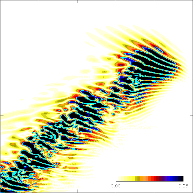
$w=12\delta$

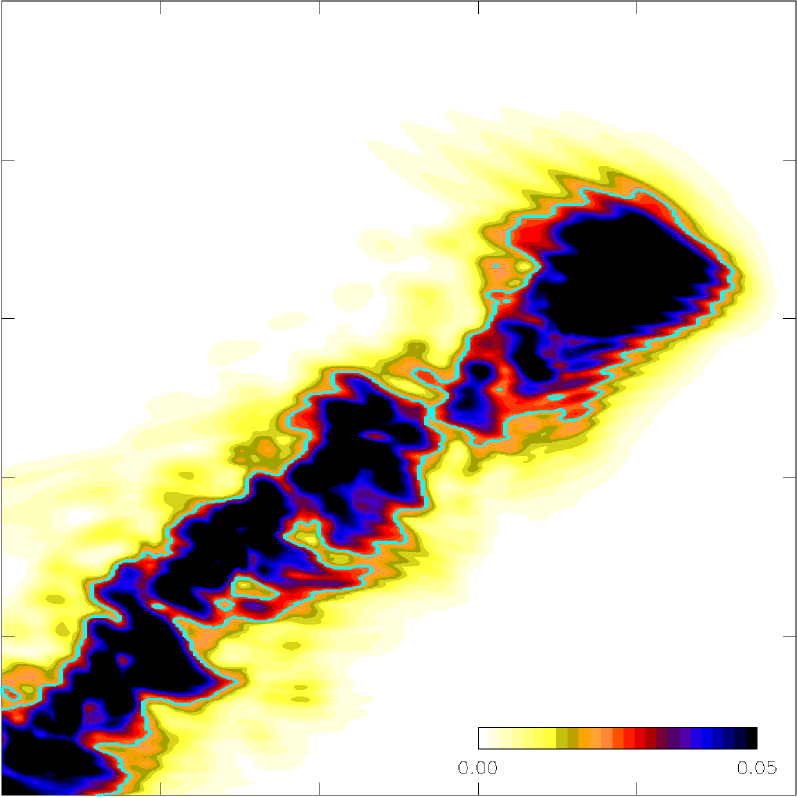
$w=40\delta$

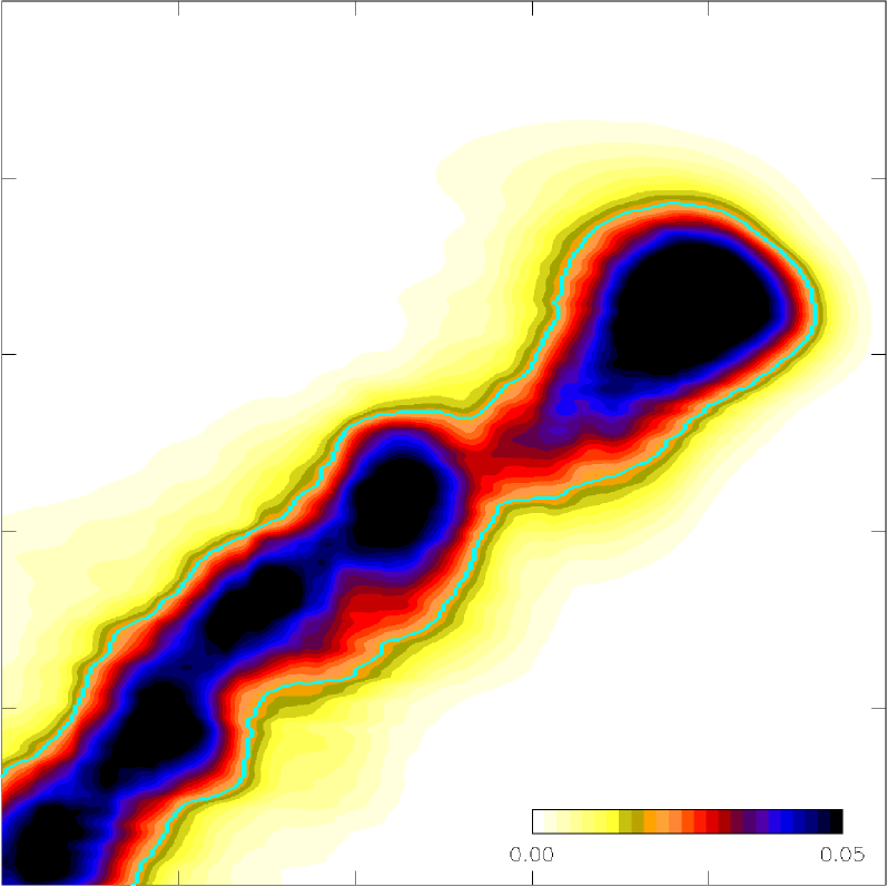
Figure 11: Color-level illustration of the DAH of the LTB shown in Fig. 8 using $|u_{y}(x,0,z)|$. The size of the domain displayed is $50\times 50\simeq 460\delta\times 460\delta$. Flow direction is from left to right. Raw data (left) and after box-filtering with the width $w=12\delta$ (routinely used here) and $w=40\delta$. Light-blue lines mark the boundaries between turbulent and laminar regions as determined by the moment-preserving thresholding method.

$\mathrm{Re}=1200$

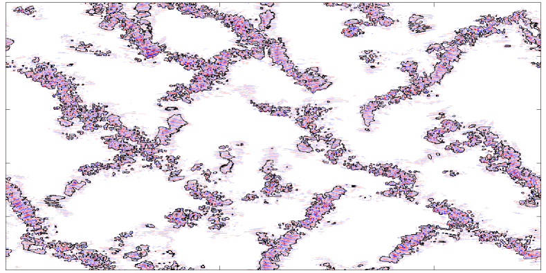
$\mathrm{Re}=1800$

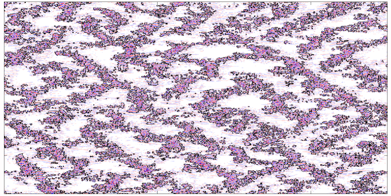
Figure 12: Moment-preserving thresholding of snapshots at $1200$ and $1800$ in Fig. 1(c,d) under box-filtering with $w=12\delta$. Flow direction is from left to right. Domain size is $500\times 250$.

Appendix C Supplemental video

Re=725

One-sided LTB regime at $\mathrm{Re}=725$ [Fig. 4(a) and (b)]. Splittings and collisions between LTBs propagating in the same direction are observed but without any trace of a transversal splitting. Wall-normal velocity field on the mid-plane $u_{y}(x,0,z,t)$ is displayed in a co-moving reference frame with velocity $0.8$ in stream-wise direction (to the right) for better visibility.

Re=850

One-sided LTB regime with rare transversal splittings at $\mathrm{Re}=850$ [Fig. 1(a)]. The displayed quantity and velocity of the reference frame are the same as in Supplemental Video Re=725.

Re=900

One-sided LTB regime with frequent transversal splittings at $\mathrm{Re}=900$ [Fig. 4(c) and (d)]. The displayed quantity and velocity of the reference frame are the same as in Supplemental Video Re=725.

Re=1050

Two-sided LTB regime at $\mathrm{Re}=1050$, slightly above the onset at $\mathrm{Re}_{2}\simeq 1011$[Fig. 1(b)]. The displayed quantity is the same as in Supplemental Video Re=725. The velocity of the reference frame is $0.7$.

Re=1200

Strongly intermittent loose continuous network of LTBs at $\mathrm{Re}=1200$ [Fig. 1(c)]. The displayed quantity is the same as in Supplemental Video Re=725. The velocity of the reference frame is $0.6$.

Re=1800

Weakly intermittent loose banded pattern at $\mathrm{Re}=1800$ [Fig. 1(d)]. The displayed quantity is the same as in Supplemental Video Re=725. The velocity of the reference frame is $0.45$.

Re=3000

Tight banded pattern at $\mathrm{Re}=3000$ [Fig. 1(e)]. The displayed quantity is the same as in Supplemental Video Re=725. The velocity of the reference frame is $0.35$.

One-sided regime in a larger domain at Re=900

Everything is same as in Supplemental Video Re=900 except for the horizontal domain size, which is 1000 and 500 in streamwise and spanwise directions respectively. The initial transient state is included to show the transition from randomly distributed LTBs of both directions to the final one-sided state.

Two-sided regime in a larger domain at Re=1050

Everything is same as in Supplemental Video Re=1050 except for the horizontal domain size, which is 1000 and 500 in streamwise and spanwise directions respectively.

References

- Huerre and Rossi (1998) Patrick Huerre and Maurice Rossi, “Hydrodynamic instabilities in open flows,” in Hydrodynamics and nonlinear instabilities, edited by Claude Godrèche and Paul Manneville (Cambridge University Press, 1998) pp. 81–294.
- Schmid and Henningson (2012) Peter J Schmid and Dan S Henningson, Stability and transition in shear flows, 2nd ed. (Springer, 2012).
- Orszag (1971) Steven A. Orszag, “Accurate solution of the Orr–Sommerfeld stability equation,” J. Fluid Mech. 50, 689–703 (1971).
- Jiménez and Moin (1991) Javier Jiménez and Parviz Moin, “The minimal flow unit in near-wall turbulence,” J. Fluid Mech. 225, 213–240 (1991).
- Waleffe (2001) Fabian Waleffe, “Exact coherent structures in channel flow,” J. Fluid Mech. 435, 93–102 (2001).
- Kawahara et al. (2012) Genta Kawahara, Marcus Uhlmann, and Lannaert van Veen, “The significance of simple invariant solutions in turbulent flows,” Annu. Rev. Fluid Mech. 44, 203–225 (2012).
- Zammert and Eckhardt (2014) Stefan Zammert and Bruno Eckhardt, “Streamwise and doubly-localized periodic orbits in plane Poiseuille flow,” J. Fluid Mech. 761, 348–359 (2014).
- Coles (1965) Donald Coles, “Transition in circular Couette flow,” J. Fluid Mech. 21, 385–425 (1965).
- Andereck et al. (1986) C. David Andereck, S.S. Liu, and Harry L. Swinney, “Flow regimes in a circular Couette flow system with independently rotating cylinders,” J. Fluid Mech. 164, 155–183 (1986).
- Prigent et al. (2003) Arnaud Prigent, Guillaume Grégoire, Hugues Chaté, and Olivier Dauchot, “Long-wavelength modulation of turbulent shear flows,” Physica D: Nonlinear Phenomena 174, 100–113 (2003).
- Tuckerman and Barkley (2011) Laurette Tuckerman and Dwight Barkley, “Patterns and dynamics in transitional plane Couette flow,” Physics of Fluids 23, 041301 (2011).
- Deusebio et al. (2014) Enrico Deusebio, Geert Brethouwer, Philipp Schlatter, and Erik Lindborg, “A numerical study of the unstratified and stratified Ekman layer,” J. Fluid Mech. 755, 672–704 (2014).
- Klotz et al. (2017) Lucasz Klotz, Grégoire Lemoult, Idalia Frontzak, Laurette S. Tuckerman, and José Eduardo Wesfreid, “Couette–Poiseuille flow experiment with zero mean advection velocity: subcritical transition to turbulence,” Phys. Rev. Fluids 2, 043904 (2017).
- Deusebio et al. (2015) Enrico Deusebio, Colm-cille P. Caulfield, and John R. Taylor, “The intermittency boundary in stratified plane Couette flow,” J. Fluid Mech. 781, 298–329 (2015).
- Tsukahara et al. (2009) Takahiro Tsukahara, Yasuo Kawaguchi, and Hiroshi Kawamura, “An experimental study on turbulent-stripe structure in transitional channel flow,” (2009) at 6th International Symposium on Turbulence, Heat and Mass Transfer, Rome, Sep. 14–18.
- Tsukahara et al. (2005) Takahiro Tsukahara, Yohji Seki, Hiroshi Kawamura, and Daisuke Tochio, “DNS of turbulent channel flow at very low Reynolds numbers,” (2005) at 4th Int. Symp. on Turbulence and Shear Flow Phenomena, Williamsburg, Jun. 27–29.
- Barkley and Tuckerman (2005) Dwight Barkley and Laurette Tuckerman, “Computational study of turbulent laminar patterns in Couette flow,” Phys. Rev. Lett. 94, 014502 (2005).
- Tuckerman et al. (2014) Laurette Tuckerman, Tobias Kreilos, Hecke Schrobsdorff, Tobias M. Schneider, and John F. Gibson, “Turbulent-laminar patterns in plane Poiseuille flow,” Phys. Fluids 26, 114103 (2014).
- Eckhardt (2009) Bruno Eckhardt, “Turbulence transition in pipe flow: 125th anniversary of the publication of Reynolds’ paper - Introduction to the Theme Issue,” Philosophical Transactions of the Royal Society A 367, 449–455 (2009).
- Avila et al. (2011) Kerstin Avila, David Moxey, Alberto de Lozar, Marc Avila, Dwight Barkley, and Björn Hof, “The onset of turbulence in pipe flow,” Science 333, 192–196 (2011).
- Tillmark and Alfredsson (1992) Nils Tillmark and P. Henrik Alfredsson, “Experiments on transition in plane Couette flow,” J. Fluid Mech. 235, 89–102 (1992).
- Carlson et al. (1982) Dale R. Carlson, Sheila E. Widnall, and Martin F. Peeters, “A flow-visualization study of transition in plane Poiseuille flow,” J. Fluid Mech. 121, 487–505 (1982).
- Lemoult et al. (2013) Grégoire Lemoult, Jean-Luc Aider, and José Eduardo Wesfreid, “Turbulent spots in a channel: large-scale flow and self-sustainability,” J. Fluid Mech. 731, R1 (2013).
- Takeishi et al. (2015) Keisuke Takeishi, Genta Kawahara, Hiroki Wakabayashi, Markus Uhlmann, and Alfredo Pinelli, “Localized turbulence structures in transitional rectangular-duct f ow,” J. Fluid Mech. 782, 368–379 (2015).
- Ishida et al. (2017) Takahiro Ishida, Yohann Duguet, and Takahiro Tsukahara, “Turbulent bifurcations in intermittent shear flows: From puffs to oblique stripes,” Phys. Rev. Fluids 2, 073902 (2017).
- Barkley and Tuckerman (2007) Dwight Barkley and Laurette Tuckerman, “Mean flow of turbulent-laminar patterns in plane Couette flow,” J. Fluid Mech. 576, 109–137 (2007).
- Pomeau (1986) Yves Pomeau, “Front motion, metastability and subcritical bifurcations in hydrodynamics,” Physica D: Nonlinear Phenomena 23, 3–11 (1986).
- Henkel et al. (2008) Malte Henkel, Haye Hinrichsen, and Sven Lübeck, Non-equilibrium phase transitions. Vol.1 (Springer, 2008).
- Barkley (2011) Dwight Barkley, “Simplifying the complexity of pipe flow,” Phys. Rev. E 84, 016309 (2011).
- Shi et al. (2013) Liang Shi, Marc Avila, and Björn Hof, “Scale invariance at the onset of turbulence in Couette flow,” Physical review letters 110, 204502 (2013).
- Lemoult et al. (2016) Grégoire Lemoult, Liang Shi, Kerstin Avila, Shreyas V Jalikop, Marc Avila, and Björn Hof, “Directed percolation phase transition to sustained turbulence in Couette flow,” Nature Physics 12, 254–258 (2016).
- Hiruta and Toh (2018) Yoshiki Hiruta and Sadayoshi Toh, “Subcritical laminar-turbulence transition with wide domains in simple two-dimensional Navier–Stokes flow without walls,” arXiv preprint arXiv:1805.04257 (2018).
- Chantry et al. (2017) Matthew Chantry, Laurette S Tuckerman, and Dwight Barkley, “Universal continuous transition to turbulence in a planar shear flow,” Journal of Fluid Mechanics 824 (2017).
- Shimizu et al. (2017) Masaki Shimizu, Genta Kawahara, and Paul Manneville, “Onset of sustained turbulence in plane Couette flow,” (2017) in 9th JSME-KSME Thermal and Fluids Engineering Conference, Okinawa, Oct. 28–30.
- Sano and Tamai (2016) Masaki Sano and Keiichi Tamai, “A universal transition to turbulence in channel flow,” Nature Physics 12, 249 (2016).
- Tao and Xiong (2013) Jianjun Tao and Xiangming Xiong, “The unified transition stages in linearly stable shear flows,” (2013) at 14th Asia Congress of Fluid Mechanics, Hanoi and Halong, Oct. 15–19.
- Xiong et al. (2015) Xiangming Xiong, Jianjun Tao, Shiyi Chen, and Luca Brandt, “Turbulent bands in plane-Poiseuille flow at moderate Reynolds numbers,” Physics of Fluids 27, 041702 (2015).
- Tsukahara and Ishida (2015) Takahiro Tsukahara and Takahiro Ishida, “Lower bound of subcritical transition in plane Poiseuille flow,” Nagare 34, 383–386 (2015).
- Kanazawa et al. (2017) Takahiro Kanazawa, Masaki Shimizu, and Genta Kawahara, “A two-dimensionally localized turbulence in plane channel flow,” (2017) at 9th JSME-KSME Thermal and Fluids Engineering Conference, Okinawa, Oct. 28–30.
- Tao et al. (2018) Jianjun Tao, Bruno Eckhardt, and Xiangming Xiong, “Extended localized structures and the onset of turbulence in channel flow,” Physical Review Fluids 3, 011902 (2018).
- Hof (2016) B Hof, “Transition to turbulence,” (2016), in Workshop on Extreme Events and Criticality in Fluid Mechanics: Computations and Analysis. The Fields Institute, Toronto, Jan. 25–29.
- Paranjape et al. (2017) Chaitanya S. Paranjape, Yohann Duguet, and Björn Hof, “Bifurcation scenario for turbulent stripes in plane Poiseuille flow,” (2017) at 16th EuropeanTurbulence Conference, Stockholm, Aug. 21–24.
- (43) See Supplemental Material at [URL will be inserted by publisher] for movies.
- Teramura and Toh (2016) Toshiki Teramura and Sadayoshi Toh, “Chaotic self-sustaining structure embedded in the turbulent-laminar interface,” Physical Review E 93, 041101(R) (2016).
- Pope (2000) Stephen B. Pope, Turbulent flows (Cambridge University Press, 2000).
- Dean (1978) Roger Bruce Dean, “Reynolds number dependence of skin friction and other bulk flow variables in two-dimensional rectangular duct flow,” Journal of Fluids Engineering 100, 215–223 (1978).
- Patel and Head (1969) V.C. Patel and M.R. Head, “Some observations on skin friction and velocity profiles in fully developed pipe and channel flows,” Journal of Fluid Mechanics 38, 181–201 (1969).
- Manneville and Shimizu (2019) Paul Manneville and Masaki Shimizu, “Subcritical transition to turbulence in wall-bounded flows: the case of plane Poiseuille flow,” in 22ème Rencontre du Non Linéaire (2019) arXiv:1904.03739.
- Shimizu et al. (2014) Masaki Shimizu, Paul Manneville, Yohann Duguet, and Genta Kawahara, “Splitting of a turbulent puff in pipe flow,” Fluid Dynamics Research 46, 061403 (2014).
- Manneville (2012) Paul Manneville, “On the growth of laminar–turbulent patterns in plane Couette flow,” Fluid Dynamics Research 44, 031412 (2012).
- Barkley (2016) Dwight Barkley, “Theoretical perspective on the route to turbulence in a pipe,” Journal of Fluid Mechanics 803 (2016).
- Shih et al. (2016) Hong-Yan Shih, Tsung-Lin Hsieh, and Nigel Goldenfeld, “Ecological collapse and the emergence of travelling waves at the onset of shear turbulence,” Nature Physics 12, 245 (2016).
- Tsai (1985) Wen-Hsiang Tsai, “Moment-preserving thresholding - A new approach,” Computer Vision Graphics and Image Processing 29, 377–393 (1985).
- (54) The agreement is qualitative because the Barkley–Tuckerman oblique geometry Barkley and Tuckerman (2005) is only appropriate for bands generated by periodic continuation at a short distance along their own direction, which (i) reinforce coherence along that direction, (ii) forbids the opening of laminar gaps and the account of LTBs around , (iii) kills orientation fluctuations and/or superpositions near , all together leading to an upward shift of the effective Reynolds number w.r. to its nominal value.
- (55) Finite-size effects linked to this methodological difference presumably roots a systematic discrepancy between our definition of the mean-flow based Reynolds number and the one in Sano and Tamai (2016), leaving us unable to match results about DP thresholds quantitatively.
- Shimizu and Manneville (2019) Masaki Shimizu and Paul Manneville, “On the decay of localized turbulent bands in channel flow,” in preparation (2019).
- Shen (1995) Jie Shen, “Efficient spectral-galerkin method ii. direct solvers of second-and fourth-order equations using Chebyshev polynomials,” SIAM Journal on Scientific Computing 16, 74–87 (1995).
- Boyd (2001) John P Boyd, Chebyshev and Fourier spectral methods (Courier Corporation, 2001).