On-demand quantum key distribution using superconducting rings with a mesoscopic Josephson junction

Abstract

We present a quantum key distribution (QKD) protocol based on long lived coherent states prepared on superconducting rings with a mesoscopic Josephson junction (dc-SQUIDs). This enables storage of the prepared states for long durations before actually performing the key distribution. Our on-demand QKD protocol is closely related to the coherent state based continuous variable quantum key distribution protocol. A detailed analysis of preparation, evolution and different measurement schemes that are required to be implemented on dc-SQUIDs to carry out the QKD is provided. We present two variants of the protocol, one requiring time stamping of states and offering a higher key rate and the other without time stamping and a lower key rate. This is a step towards having non-photon based QKD protocols which will be eventually desirable as photon states cannot be stored for long and therefore the key distribution has to be implemented immediately after photon exchange has occurred. Our protocol offers an innovative scheme to perform QKD and can be realized using current experimental techniques.

I Introduction

In the quantum world the joint measurement of non-commuting observables is impossible and if attempted, leads to the introduction of disturbances in the measured outcomes for both. This fundamental feature of quantum physics was exploited by Bennett and Brassard to invent a secure key distribution protocol for cryptography Bennett and Brassard (1984); Bennett (1992). Unlike classical key distribution schemes where the security is based on ‘a hard to solve mathematical problem’, security of quantum key distribution (QKD) protocols is based on laws of nature which cannot be violated Gisin et al. (2002); Shor and Preskill (2000); Branciard et al. (2005). Subsequently, other key quantum features, like entanglement Gisin et al. (2002), Bell-nonlocality Ekert (1991); Acín et al. (2006), no-cloning theorem Cerf et al. (2002); Ralph (1999) and monogamy of quantum correlations Pawłowski (2010); Singh et al. (2017) have also been employed to show unconditional security Scarani et al. (2009); Ralph (2000); Grosshans and Grangier (2002) of discrete and continuous variable QKD protocols.

The experimental realizations of QKD protocols have primarily been on light and optical devices Grosshans et al. (2003); Takesue et al. (2007); Fedrizzi et al. (2009); Jouguet et al. (2013); Takenaka et al. (2017). While the optical setup has many advantages, it imposes a serious constraint: Bob has to perform his chosen measurement immediately once he receives the state because it is not possible to store photonic states for long durations. In this paper we develop a novel way to perform QKD in which Bob is not under any compulsion to perform measurements as soon as the states are exchanged. Bob may choose to store the states until the need for key distribution arises, at which time he performs measurements, exchanges classical information with Alice and generates the key. The proposed protocol is a continuous variable QKD based on superconducting rings with a Josephson junction Joshi (2000); Everitt et al. (2001); Fagaly (2006). This system, known as dc-SQUIDs, allows for preparation of extremely long lived continuous variable coherent states under no-dissipation conditions Zou and Shao (1999, 2001). These states can be stored as such indefinitely at equilibrium, which ensures a dissipationless situation Friedman et al. (2000). For sufficiently low temperatures, a persistent current has been shown to exist in these families of superconducting rings with mesoscopic Josephson junctions Mailly et al. (1993); Lévy et al. (1990)

The protocol involves preparing arbitrary coherent states of the dc-SQUID by Alice, which are then transported to Bob. Bob stores these states for as long as he wants, during which time these states evolve under the system Hamiltonian. Bob undertakes measurements on these dc-SQUID states when he wants to generate the key. We find that the states during the storage time undergo collapse and revival phenomena due to the presence of a nonlinear term in the Hamiltonian. Given this, two distinct measurement schemes are possible, either of which can implemented by Bob to generate the key. In the first scheme, Bob measures at an arbitrary time and in the second scheme, he measures at specified time intervals to maximize the secure key rate. The second measurement scheme requires time stamping, i. e. Alice and Bob have to share a clock and a precise time of preparation of the coherent state needs to be marked on each dc-SQUID. We show that a secure key rate of $0.20$ bits and $0.50$ bits can be achieved for the schemes, respectively. Finally, we show that the protocol is secure against an eavesdropper under the assumption of individual attacks. The new feature of the protocol is the possibility of storing the dc-SQUID, prepared in a coherent state, in Bob’s lab for long durations and the use of a non-photonic system for QKD. The proposed protocol can be implemented using current superconducting technologies. Since the QKD can be carried out at any time after state exchange, we call our protocol as on-demand QKD.

The paper is organized as follows: In Section II.1 we briefly introduce the concept of continuous variable quantum key distribution (CV-QKD) with a focus on coherent states, while in Section II.2 we review basic concepts of superconductivity as pertaining to superconducting rings with a mesoscopic Josephson junction. We describe the preparation and evolution of these states in some details in Sections II.3 and II.4. In Section III we describe our QKD protocol while in Section IV we prove its security. In Section V we provide some concluding remarks.

II Background

II.1 Coherent state based CV-QKD

In this section we provide a brief introduction to CV-QKD with a focus on the coherent state protocol as detailed in Grosshans and Grangier (2002). We sketch out the protocol and briefly analyze the security considerations.

Consider two parties Alice and Bob who wish to share a secret key using a coherent state based QKD protocol. Alice randomly draws two numbers $x_{A}$ and $p_{A}$ from two Gaussian distributions with the same variance $V_{A}N_{0}$, where $N_{0}=1$ is the vacuum noise variance. She then prepares the coherent state $|x_{A}+ip_{A}\rangle$ and transmits it to Bob through a channel with Gaussian and white noise. Upon receiving the state, Bob randomly chooses to perform a homodyne measurement of either $X$ (position) or $P$ (momentum) quadrature.

Through a classically authenticated channel Bob reveals his choices of measurement quadratures to Alice, who then rejects the random number not corresponding to the measured quadrature. The procedure is repeated a large number of times and the random number with Alice and the outcome with Bob is kept as part of the raw key. In the end, Alice and Bob can use the sliced reconciliation protocol Cerf et al. (2002) to transform their raw key into errorless bit strings from which a secure key can be distilled by privacy amplification.

If we consider the presence of an eavesdropper, Eve in the channel, a secret key can be distilled from the protocol only if

$$r_{\text{min}}=I(A:B)-I(A:E)>0,$$ (1)

where $I(A:B)$ and $I(A:E)$ represent the mutual information between Alice and Bob and Alice and Eve respectively and $r_{\text{min}}$ is the minimum rate at which a secure key can be distilled. Eqn. (1) physically implies that a secure key can be distilled only when the information shared between Alice and Bob is strictly greater than the information shared between Alice and Eve.

From a result in Shannon (1948), it can be shown that if the signal and noise have Gaussian statistics, the optimum information rate achievable between Alice and Bob is

$$I(A:B)=\frac{1}{2}\log_{2}(1+\Sigma_{B}).$$ (2)

where $\Sigma_{B}$ is the signal-to-noise ratio (SNR) as measured by Bob. To evaluate the maximum information about Alice’s key gleaned by Eve, it is required to ascribe the best physically possible strategy to her. If the transmission line between Alice and Bob has transmittivity $\eta$, Eve can then employ a strategy wherein she captures a fraction $1-\eta$ of the beam and transmits the fraction $\eta$ to Bob through her own lossless line. This way she gains maximum amount of information.

A general result proven in Grosshans and Grangier (2001) demonstrates that if the added noise on Bob’s side is $\chi N_{0}$, the minimum added noise on Eve’s side is $\chi^{-1}N_{0}$, where $\chi={(1-\eta)}/{\eta}$. The above is a consequence of the no-cloning theorem and can be applied to show security of the aforementioned protocol when Eve performs individual attacks.

In the case of the coherent state protocol, the total variance of the beam leaving Alice’s site is $VN_{0}=V_{A}N_{0}+N_{0}$. The security condition (1) then reads as

$$r_{\text{min}} =\frac{1}{2}\log_{2}(1+\Sigma_{B})-\frac{1}{2}\log_{2}(1+\Sigma_{E})$$ (3)

$$=\frac{1}{2}\log_{2}\left(\frac{V+\chi}{1+V\chi}\right),$$

where we have used

$$1+\Sigma_{B}=\frac{V+\chi}{1+\chi},\quad 1+\Sigma_{E}=\frac{V+1/\chi}{1+1/\chi}.$$ (4)

From Eqn. (3) it is seen that a secure key can be distilled if $\chi<1$. This further puts bounds on the transmittivity $\eta>\frac{1}{2}$. In other words, as long as Alice-Bob channel transmission efficiency is greater than 50%, they can successfully carry out QKD.

II.2 Superconducting ring with a junction (dc-SQUID)

Figure 1: A superconducting ring of inductance $L$ with a mesoscopic Josephson junction with capacitance $C$. The Josephson coupling constant is $E_{J}$ and $\phi_{x}$ is the external flux.

In this section we provide a brief background to superconducting rings with a mesoscopic Josephson junction, also termed as a dc-SQUID. We mainly focus on preparation of coherent quantum states Zou and Shao (1999, 2001) and their evolution on a dc-SQUID which is essential for our protocol.

Consider a superconducting ring of inductance $L$ with a Josephson junction with capacitance $C$ and external inductive coupling through an external flux $\phi_{x}$, as shown in Fig. 1. The quantum Hamiltonian for the junction can be written as,

$$H=\frac{Q^{2}}{2C}+\frac{(\Phi^{\prime}-{\phi}_{x})^{2}}{2L}+E_{J}(1-\cos\theta),$$ (5)

where we have taken $\hbar=k_{B}=c=1$. The quantity $Q$ is the charge operator across the junction and $\Phi^{\prime}$ is the operator corresponding to the total flux through the ring. The quantity $E_{J}$ is the Josephson coupling constant and $\theta$ is the phase difference of the superconducting wavefunction across the junction. The phase difference $\theta$ is related to the total flux $\Phi^{\prime}$ by $\theta=2e\Phi^{\prime}$. The quantum mechanical operators, $Q$ and $\Phi^{\prime}$ form a canonically conjugate pair of variables with the canonical commutation relationship

$$\left[\Phi^{\prime},Q\right]=i.$$ (6)

The commutation relation can be rewritten in terms of voltage across the junction, $V^{\prime}=Q/C$ as,

$$C\left[\Phi^{\prime},V^{\prime}\right]=i.$$ (7)

Due to experimental considerations, in the remainder of this paper we treat $V^{\prime}$ and $\Phi^{\prime}$ equivalent to the continuous variable quantum mechanical quadrature operators rather than $Q$ and $\Phi^{\prime}$, as is evident from Eqn. (7). The corresponding uncertainty relationship for the $V^{\prime}$ and $\Phi^{\prime}$ quadratures is,

$$\langle\left(\Delta\Phi^{\prime}\right)^{2}\rangle\langle\left(\Delta V^{\prime}\right)^{2}\rangle\geq\frac{1}{4C^{2}}.$$ (8)

The Hamiltonian for a dc-SQUID (5) is found to be equivalent to that of a simple harmonic oscillator with an additional coupling term proportional to the Josephson coupling energy. The first term corresponds to kinetic energy and the last two terms correspond to potential energy.

Expanding the last term in the Hamiltonian (5) and retaining terms upto the fourth order in $\theta$, we get,

$$H = \frac{Q^{2}}{2C}+\frac{C}{2}\omega^{2}\Phi^{\prime 2}-\frac{\Phi^{\prime}\phi_{x}}{L}-\frac{2}{3}E_{J}e^{4}{\Phi^{\prime}}^{4},$$ (9)

$${\rm with}\quad\omega=\left(\frac{1}{CL}+\frac{4e^{2}E_{J}}{C}\right)^{\frac{1}{2}}.$$

To simplify calculations we work with the dimensionless quadratures defined as,

$$\Phi=\sqrt{C\omega}\Phi^{\prime}\quad\text{and}\quad V=\sqrt{\frac{C}{\omega}}V^{\prime}$$ (10)

The creation and annihilation operators, $b$ and $b^{\dagger}$ can then be introduced as:

$$\Phi=\frac{1}{\sqrt{2}}(b+b^{\dagger}),\quad V=\frac{i}{\sqrt{2}}(b^{\dagger}-b).$$ (11)

In the rotating wave approximation and neglecting all the terms without annihilation and creation operators, Eqn. (9) can be re-written as,

$$H=\Omega b^{\dagger}b-\mu(b+b^{\dagger})-\nu(b^{\dagger}b)^{2},$$ (12)

where

$$\nu=\frac{2E_{J}e^{4}}{3(\omega C)^{2}},\quad\mu=\frac{\phi_{x}}{L\sqrt{2\omega C}},\quad\Omega=\omega-\nu.$$ (13)

The second term in the Hamiltonian (12) depends on the external driving flux $\phi_{x}$, which can be switched on for a short duration $\tau_{1}$ when desired. The strength of the driving flux is appropriately chosen such that $\mu\gg\Omega,\nu$ for the duration when it is turned on. We further impose the experimentally achievable condition $\Omega\gg\nu$ and for the remainder of the paper work in the regime $\mu\gg\Omega\gg\nu$ Zou and Shao (1999, 2001).

For the duration $\tau_{1}$ when the driving field is turned on, only the second term of the Hamiltonian (12) is relevant and it effectively generates a phase space displacement of the ground state and its corresponding unitary operator can be written as

$$D(\tau_{1})=\text{e}^{i\mu(b+b^{\dagger})\tau_{1}},$$ (14)

By a suitable choice of the external driving field $\phi_{x}$ and time durations $\tau_{1}$, we can modulate the value of $\mu$ and prepare an arbitrary coherent state. However, it should be noted that $\mu$ is real and thus the corresponding displacement operator (14) will displace the ground state of the junction only along the $V$ quadrature.

After the driving field is switched off, the Hamiltonian consists of only the first and the third term. From the condition $\Omega\gg\nu$, for a short duration $\tau_{2}$ the first term dominates and the effective Hamiltonian is responsible for generating a phase shift which corresponds to a phase space rotation with unitary operator given as

$$R(\tau_{2})=\text{e}^{-i\Omega b^{\dagger}b\tau_{2}}.$$ (15)

For a long storage time duration $\tau_{3}$, the external field is switched off and the third term in the Hamiltonian (12) becomes significant alongwith the first term. In the interaction picture where the first terms gets absorbed, the unitary operator corresponding to the Hamiltonian for the storage period is,

$$S(\tau_{3})=\text{e}^{i\nu(b^{\dagger}b)^{2}\tau_{3}}.$$ (16)

The effect of the third non-linear term is to squeeze and de-squeeze the coherent states of the Josephson junction in the $V$ and $\Phi$ quadrature resulting in a collapse and revival phenomenon. The system starts out in a coherent state which then gets squeezed by the nonlinear term. At time $\tau_{3}=\frac{\pi}{\nu}$ the squeezing vanishes and the resultant state is $|-\alpha\rangle$, as will be shown in Section II.4, which is just the initial coherent state rotated by an angle $\pi$. As time elapses, the state is again squeezed and at a time $\tau_{3}=\frac{2\pi}{\nu}$ the squeezing again vanishes and the resultant state is found to be $|\alpha\rangle$, which is exactly the initial coherent state. This cycle of collapse and revival continues indefinitely under no-dissipation conditions. In between, we also see superposition of two coherent states.

II.3 Preparation of coherent states on a dc-SQUID

Alice can prepare the chosen coherent state $|\phi_{A}+iv_{A}\rangle$ on a dc-SQUID by first preparing it in the ground state $|0\rangle$. This can be achieved by allowing the SQUID to decohere to its ground state in the low Josephson coupling limit Everitt et al. (2004). By appropriately choosing the magnitude of the driving field $\phi_{x}$, Alice applies the displacement operator for a short duration $\tau_{1}$, given by Eqn. (14), on the ground state to get:

$$D\left(\frac{\phi_{A}}{\mu_{1}}\right)|0\rangle=|0+i\phi_{A}\rangle.$$ (17)

Since $\mu_{1}$ is a real quantity, the state is displaced only along the $V$ quadrature. The driving field is then switched off for a time $\tau_{2}$ such that $\Omega\tau_{2}=\pi/2$ which results in rotating the quadratures of the coherent state by an angle $\pi/2$:

$$R\left(\frac{\pi}{2\Omega}\right)|0+i\phi_{A}\rangle=|\phi_{A}+0\rangle.$$ (18)

Since $\tau_{2}$ is quite small, the nonlinear term in (12) can be ignored as we have $\Omega\gg\nu$. The resultant state is then once again displaced along the $V$ quadrature by appropriately choosing the magnitude of the driving field for a short duration $\tau_{1}$:

$$D\left(\frac{v_{A}}{\mu_{2}}\right)|\phi_{A}+0\rangle=|\phi_{A}+iv_{A}\rangle.$$ (19)

The entire procedure can be summarized by an application of the operator $T(\phi_{A},v_{A})$ on the ground state of the dc-SQUID as,

$$T(\phi_{A},v_{A})=D\left(\frac{v_{A}}{\mu_{2}}\right)R\left(\frac{\pi}{2\Omega}\right)D\left(\frac{\phi_{A}}{\mu_{1}}\right).$$ (20)

The operator $T(\phi_{A},v_{A})$ depends on the structural properties of the junction, the applied external driving field and the time durations $\tau_{1}$ and $\tau_{2}$. By appropriately choosing these values a dc-SQUID can be prepared in an arbitrary coherent state as required.

Figure 2: ($a$) Solid line represents the variance of $\Phi$ quadrature while the dashed line represents variance of $V$ quadrature. The condition for squeezing in quadrature $X$ is $\langle(\Delta X)^{2}\rangle<1/2$. It can be seen that while one quadrature is squeezed, its conjugate is de-squeezed.($b$) For state (22) the product of the variance is always greater than 1/4 except when the state revives to a coherent state. To clearly show squeezing and desqueezing of quadratures, we have taken $\Omega=5\nu$, $\phi_{A}=0.3$ and $v_{A}=0.3$.

II.4 Evolution of coherent states under storage

After state preparation, as we will shall see in Section III, Alice needs to transfer the ensemble of dc-SQUIDs to Bob, who then stores it. During the storage period, the term corresponding to applied external field is zero and the effective Hamiltonian takes the form:

$$H=\Omega b^{\dagger}b-\nu(b^{\dagger}b)^{2}.$$ (21)

Storing the dc-SQUID under no-dissipation conditions for a large time $\tau_{3}$ results in both the phase and the non-linear term in Eqn. (21) contributing significantly to the evolution of the state. Let us consider the state at time $t=0$ to be $|\alpha\rangle=|\phi_{A}+iv_{A}\rangle$, then the resultant state at a later time $t$ is

$$|\psi(t)\rangle=\text{e}^{-i\Omega b^{\dagger}bt}\text{e}^{i\nu(b^{\dagger}b)^{2}t}|\alpha\rangle.$$ (22)

In Fock state basis, Eqn. (22) becomes

$$|\psi(t)\rangle=e^{-\frac{|\alpha|^{2}}{2}}\sum_{n=0}^{\infty}e^{i\nu n^{2}t}\frac{(\alpha e^{-i\Omega t})^{n}}{\sqrt{n!}}|n\rangle.$$ (23)

If we engineer the value of $\Omega/\nu$ to be an even integer, the state (23) revives back to a coherent state $|-\alpha\rangle$ at time $t=\pi/\nu$. Furthermore, at time $t=2\pi/\nu$, the state evolves back to the original state $|\alpha\rangle$. As a general case, whenever $t=\pi p/\nu q$, where $p<q$ are both mutually prime, the state (23) can be written as a superposition of coherent states having the same magnitude $|\alpha|$ but differing in phase Banerji (2001); Hannay and Berry (1980):

$$|\psi\left(t=\frac{\pi p}{\nu q}\right)\rangle = \sum_{l=0}^{m-1}c_{l}^{p,q}|\alpha\text{e}^{-i\pi\left(\frac{\Omega p}{\nu q}-\frac{2l}{m}\right)}\rangle,$$

$${\rm with} c_{l}^{p,q}=\frac{1}{m}\sum_{r=0}^{m-1}\text{e}^{i\pi r\left(\frac{pr}{q}-\frac{2l}{m}\right)}$$ (24)

and $m=q$ if at most one of $p$ or $q$ is odd and $m=2q$ if both are odd. For the values $p=1$ and $q=2$, Eqn. (24), reduces to a superposition of two coherent states as,

$$|\psi\left(t=\frac{\pi}{2\nu}\right)\rangle = \frac{1}{\sqrt{2}}\left[\text{e}^{i(\pi/4)}|\alpha\text{e}^{-i\Omega\pi/2\nu}\rangle\right.$$ (25)

$$\left.+\text{e}^{-i(\pi/4)}|-\alpha\text{e}^{-i\Omega\pi/2\nu}\rangle\right].$$

The variance in either quadrature for the state (22) can be calculated and is given as

$$\langle(\Delta\Phi)^{2}\rangle = \frac{1}{2}\left[1+2|\alpha|^{2}+\alpha^{2}\text{e}^{\left(|\alpha|^{2}\left(\gamma^{2}-1\right)-2it\xi\right)}\right.$$ (26)

$$-\beta^{2}\text{e}^{\left(|\alpha|^{2}\left(\gamma^{-2}-1\right)+2it\xi\right)}$$

$$\left.\!\!\!\!\!\!\!\!\!\!\!\!\!\!\!\!\!\!\!\!\!\!\!\!\!\!+\text{e}^{-2it\zeta}\left(\beta^{*}\text{e}^{\left(|\alpha|^{2}\left(\gamma-1\right)\right)}-\beta\text{e}^{\left(|\alpha|^{2}\left(\gamma^{-1}-1\right)+2it\zeta\right)}\right)^{2}\right],$$

$$\langle(\Delta V)^{2}\rangle = \frac{1}{2}\left[1+2|\alpha|^{2}-\alpha^{2}\text{e}^{\left(|\alpha|^{2}\left(\gamma^{2}-1\right)-2it\xi\right)}\right.$$ (27)

$$+\beta^{2}\text{e}^{\left(|\alpha|^{2}\left(\gamma^{-2}-1\right)+2it\xi\right)}$$

$$\!\!\!\!\!\!\!\!\!\!\!\!\!\!\!\!\!\!\!\!\!\!\!\!\!\!\left.-\text{e}^{-2it\zeta}\left(\beta^{*}\text{e}^{\left(|\alpha|^{2}\left(\gamma-1\right)\right)}+\beta\text{e}^{\left(|\alpha|^{2}\left(\gamma^{-1}-1\right)+2it\zeta\right)}\right)^{2}\right],$$

where $\alpha=(\phi+iv)/\sqrt{2}$, $\xi=\Omega-2\nu$, $\beta=(v+i\phi)/\sqrt{2}$, $\gamma=\text{e}^{2i\nu t}$ and $\zeta=\Omega-\nu$. A state is said to be squeezed in quadrature $X\in\{\Phi,V\}$ if its variance $\langle(\Delta X)^{2}\rangle<1/2$. Fig. 2 shows the plot of variance of both $\Phi$ and $V$ quadrature with time and their product showing the appearance and disappearance of squeezing with time. While the product of variances obey the uncertainty principle given in Eqn. (8), the squeezing appears when one of the variances falls below the coherent state value.

As a special case, we analyze squeezing for the state (25). For this case Eqn. (26) and Eqn. (27) yield

$$\langle(\Delta\Phi)^{2}\rangle=\begin{cases}\frac{1}{2}+\phi^{2}-\text{e}^{-2(\phi^{2}+v^{2})}v^{2}&\frac{\Omega}{\nu}~{}\text{is even},\\ \frac{1}{2}+v^{2}-\text{e}^{-2(\phi^{2}+v^{2})}\phi^{2}&\frac{\Omega}{\nu}~{}\text{is odd}\end{cases}$$ (28)

$$\langle(\Delta V)^{2}\rangle=\begin{cases}\frac{1}{2}+v^{2}-\text{e}^{-2(\phi^{2}+v^{2})}\phi^{2}&\frac{\Omega}{\nu}~{}\text{is even},\\ \frac{1}{2}+\phi^{2}-\text{e}^{-2(\phi^{2}+v^{2})}v^{2}&\frac{\Omega}{\nu}~{}\text{is odd }\end{cases}$$ (29)

Fig. 3 shows a contour plot for when $\Omega/\nu$ is even. The state is found to be squeezed for only a finite region of $\Phi$ and $V$ inside a contour value of $0.50$.

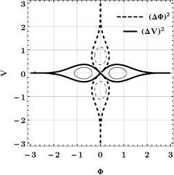
Figure 3: Thick-solid and thick-dashed curves represent a contour of value $0.5$ while thin-solid and thin-dashed curves represent a contour of value $0.4$. For points inside contour value $0.5$, state (25) is squeezed in $\Phi$ and $V$ while for points outside this contour there is no second order squeezing.

Therefore, we see that the stored coherent state undergoes collapse and revival, directly affecting the correlations between Alice and Bob. In the succeeding subsections, we analyze two different measurement schemes by Bob and calculate the average key rate for both the cases.

III Protocol

Figure 4: ($a$) Preparation of the desired coherent state, by displacing the ground state from A to B followed by a rotation to C and a subsequent displacement to D. ($b$) Collapse and revival of the state in the $\Phi$ quadrature when kept in storage for long durations. We have taken values $\Omega=20\nu$ for the purpose of clarity and $\phi_{A}=0.3$, $v_{A}=0$. ($c$) Measurement of the state by Bob by randomly choosing a quadrature from either $V$ or $\Phi$.

In this section we describe our on-demand QKD protocol based on coherent states prepared on a dc-SQUID. The key distribution protocol involves following stages:

• Alice randomly samples two numbers $\phi_{A}$ and $v_{A}$ from two Gaussian distributions with the same variance $V_{A}N_{0}$ and means at $\phi_{0}$, $v_{0}$, respectively and prepares the coherent state $|\phi_{A}+iv_{A}\rangle$ on a dc-SQUID as described in Section II.3. She repeats and prepares an ensemble of dc-SQUIDs in coherent states with $\phi_{A}$ and $v_{A}$ chosen randomly from a Gaussian distribution respectively.

• Alice transfers this numbered ensemble of dc-SQUIDS to Bob via a channel with Gaussian noise. The numbers of SQUID elements in the ensemble are known to both Alice and Bob.

• Bob stores the ensemble after receiving it until a time when he wants to carry out QKD with Alice. During this storage period, the states of the members of the SQUIDs ensemble evolve under the system Hamiltonian and undergo collapse and revival as described in Section II.4.

• At a later time, when the demand for key distribution arises, Bob performs measurements of one of either voltage $V$ quadrature or flux $\Phi$ quadrature chosen randomly, on each numbered member of the ensemble.

• Afterwards, Bob publicly communicates his choice of measurement on each of the SQUIDs to Alice. On her side, Alice only keeps data for each SQUID corresponding to Bob’s measurement quadrature. The correlated data is thus generated.

• The correlated data is transformed into errorless bit strings by using sliced reconciliation protocols detailed in Grosshans and Grangier (2002); Cerf et al. (2002). Finally they perform privacy amplification to distill a secure key. Fig. 4 illustrates the protocol schematically.

In the step S4 above Bob can employ two different measurements schemes, one in which he does not care about the precise time for which storage was done and begins to measure the dc-SQUID quadratures at a time of his choice and the other in which time stamping is used where when he begins measurements he uses a specific time for each dc-SQUID to maximize his correlation with Alice. For both the cases we find out the average correlations that can be shared between Alice and Bob. As we shall see it is possible to carry out QKD in both the cases while the measurement scheme with specific time measurements has much higher key rate.

Case 1: Measurement at an arbitrary time

In this scheme, Bob, after the storage period performs measurement of either the $\Phi$ or $V$ quadrature without worrying about the exact time that has elapsed for each dc-SQUID after its state preparation. As has been seen in Section II.4, the non-linear evolution of the state, leads to a periodic variation of correlation between Alice and Bob as the states undergo periodic collapses and revivals. Bob’s measurement in this case is not sensitive to this process and gets implement at some random time during this cycle. Therefore, we assume that the measurement times are uniformly distributed over the interval $t=0$ and $t=2\pi/\nu$. Thus, for this case the relevant correlations is the time average correlations over this time. We calculate this correlation and the corresponding key rate that can be achieved when Bob measures each dc-SQUID at a random time. To that end, we define a quantity $C_{AB}(X)$ which quantifies the noise observed by Bob given the information encoded by Alice when a measurement of $X$ quadrature is performed,

$$C_{AB}(X) =\langle(X^{B}-X^{A})^{2}\rangle$$ (30)

$$=\langle(X^{B})^{2}\rangle+(X^{A})^{2}-2X^{A}\langle X^{B}\rangle,$$

where the average is taken over the measurement results of Bob, and $X^{A}$ and $X^{B}$ denote the information encoded by Alice and measurement result of Bob in the $X$ quadrature.

If the state prepared by Alice is $|\alpha\rangle$ upon which Bob performs a measurement at a random time $t$, the noise $C_{AB}(X)$ in the two quadratures is found to be

$$C_{AB}(\Phi) =\frac{1}{2}\left[1+2|\alpha|^{2}+4\left(\text{Re}\left(\alpha\right)\right)^{2}\right.$$ (31)

$$\!\!\!\!-4\text{Re}\left(\alpha\right)\text{e}^{-it\zeta}\left[\alpha\text{e}^{|\alpha|^{2}\left(\gamma-1\right)}+\alpha^{*}\text{e}^{\left(|\alpha|^{2}\left(\gamma^{-1}-1\right)+2it\zeta\right)}\right]$$

$$\!\!\!\!\left.+\alpha^{2}\text{e}^{|\alpha|^{2}\left(\gamma^{2}-1\right)-2it\xi}-\beta^{2}\text{e}^{\left(|\alpha|^{2}\left(\gamma^{-2}-1\right)+2it\xi\right)}\right],$$

$$C_{AB}(V) =\frac{1}{2}\left[1+2|\alpha|^{2}+4\left(\text{Im}\left(\alpha\right)\right)^{2}\right.$$ (32)

$$\!\!\!\!\!\!\!-4\text{Im}\left(\alpha\right)\text{e}^{-it\zeta}\left[\beta\text{e}^{\left(|\alpha|^{2}\left(\gamma^{-1}-1\right)+2it\zeta\right)}+\beta^{*}\text{e}^{|\alpha|^{2}\left(\gamma-1\right)}\right]$$

$$\!\!\!\!\!\!\left.-\alpha^{2}\text{e}^{\left(|\alpha|^{2}\left(\gamma^{2}-1\right)-2it\xi\right)}+\beta^{2}\text{e}^{\left(|\alpha|^{2}\left(\gamma^{-2}-1\right)+2it\xi\right)}\right].$$

where $\alpha=(\phi_{A}+iv_{A})/\sqrt{2}$, $\xi=\Omega-2\nu$, $\beta=(v_{A}+i\phi_{A})/\sqrt{2}$, $\gamma=\text{e}^{2i\nu t}$ and $\zeta=\Omega-\nu$. Let us consider that Alice randomly samples $\phi_{A}$ and $v_{A}$ from a Gaussian distribution with variance $V_{A}N_{0}=1/2$ and $\phi_{0}=v_{0}=0$. The weighted average noise observed by Bob in quadrature $X$ over all such states $\{|\alpha\rangle\}$ randomly chosen by Alice is then given as

$$C_{AB}^{\{|\alpha\rangle\}}(X) = \int_{-\infty}^{\infty}\int_{-\infty}^{\infty}dx_{1}dx_{2}\frac{1}{\pi}\text{e}^{-(x_{1}^{2}+x_{2}^{2})}C_{AB}(X)$$

$$\!\!\!\!\!\!\!\!\!\!\!\!\!\!\!\!\!\!\!\!\!\!\!\!\!\!\!\!\!\!\!\!\!=\frac{3}{2}-\frac{9\cos(t(\nu-\Omega))-6\cos(t(\nu+\Omega))+\cos(t(3\nu+\Omega))}{(5-3\cos(2\nu t))^{2}},$$

where $X$ can be either of the quadratures and the expression is same for both the quadratures. Fig. 5 shows the plots of $C_{AB}^{\{|\alpha\rangle\}}(X)$ for odd and even values of $\Omega/\nu$.

Figure 5: ($a$) Represents the error in either quadrature for $\Omega=5\nu$. When $\Omega/\nu$ is odd, the state (22) at time $t=0$, $\pi/\nu$ and $2\pi/\nu$ is $|\alpha\rangle$ and hence, noise in each case is equal to $1/2$. ($b$) Represents the error in either quadrature for $\Omega=6\nu$. When $\Omega/\nu$ is even, the state (22) at time $t=0$, and $2\pi/\nu$ is $|\alpha\rangle$ and noise in both the cases is equal to $1/2$. However, at time $\pi/\nu$, the state is $|-\alpha\rangle$ and hence, the noise is maximum.

Finally, under the approximation $\Omega\gg\nu$, we average the noise over the time period $t=0$ to $t=2\pi/\nu$ to get

$$C_{AB}^{\text{T}}(X)=\frac{\nu}{2\pi}\int_{0}^{\frac{2\pi}{\nu}}dt~{}C_{AB}^{\{|\alpha\rangle\}}(X)=\frac{3}{2},$$ (34)

and the average correlation between Alice and Bob $I(A:B)$ can be evaluated as

$$I(A:B)=\frac{1}{2}\log_{2}\left(1+\frac{V_{A}N_{0}}{C_{AB}^{\text{T}}(X)}\right).$$ (35)

For $V_{A}N_{0}=1/2$ and $C_{AB}^{\text{T}}(X)$ as given by Eqn. (34) the average correlation comes out to be $I(A:B)=0.20$ bits. The protocol thus achieves its goal of generating data that can be converted into a key by reconcilliation and privacy amplification.

Case 2: Measurements at specific times

In this scheme, upon the need for QKD, Bob performs the measurements of $\phi$ or $V$ at specific times chosen to maximize his correlation with Alice. These times correspond to the times when the state (22) reverts to a pure coherent state ($|\alpha\rangle$ or $|-\alpha\rangle$) or an equal superposition of them as given by Eqn. (25). The time scale of oscillations of states are expected to be much smaller compared to the long storage time. This time keeping has to be done for each dc-SQUID and therefore we assume that Alice does precise time stamping for each dc-SQUID. There has to be synchronization of very precise clocks between Alice and Bob in order to decide on the measurement times.

For this scheme, Alice chooses her Gaussian distribution with variance $V_{A}N_{0}=1/2$, but centered around a large value, e.g. $q_{0}=p_{0}=4$. Bob also utilizes a slightly different scheme for measurements. Apart from measuring at specified times, he takes the absolute value of the outcomes he observes. For both the cases when $\Omega/\nu$ is an odd or an even integer and Bob records only the absolute values of his outcomes, the statistics as observed by him for states at time $t=0$, $t=\pi/2\nu$, $t=\pi/\nu$, $t=3\pi/2\nu$ and $t=2\pi/\nu$ will have the same mean and variance as Alice’s. As is shown in Fig. 6 he has a bimodal distribution for the times $t=\pi/2\nu$ and $t=3\pi/2\nu$ which gets folded onto the positive side when we take the absolute value. For the rest of the times he gets the same statistics as Alice’s state $|\alpha\rangle$ after taking the absolute value. This is the reason that Alice needs to generate states with large displacement on her side for this protocol to work.

Figure 6: The probability distribution of the state (25) when Alice Gaussian distribution is centered about $q_{0}=p_{0}=4$ and $\Omega=100\nu$.

The average noise (34) for this measurement scheme by Bob at these specific time intervals is only the vacuum noise $N_{0}=1/2$. The average correlations can then be computed as

$$I(A:B)=\frac{1}{2}\log_{2}\left(1+\frac{V_{A}N_{0}}{N_{0}}\right)=0.50~{}\text{bits}.$$ (36)

As has been emphasized, in order to achieve the aforementioned correlations, it is essential to perform measurements at the precisely specified times. Since Bob will be storing these SQUIDs for a long time, it is also required to keep an accurate track of time for each and every SQUID. From an experimental point of view we can assume that the collapse and revival time period lies in the range of a few hundred microseconds $(10^{-4}$s) corresponding to $\Omega\approx 10^{4}$Hz and $\Omega/\nu=100$. Commercially available atomic clocks can keep track of time upto an error of $0.1\mu$s per day amounting to $1000$ days until the error becomes significant. Furthermore, with the current computer processors in the range of GHz, it is possible to perform precise measurements with a resolution of nanoseconds. Therefore the correlations (36) are achievable with the current technology for storage times of approximately $30$ months.

IV Security

We analyze security of the protocol for both the cases (with and without time stamping) under an assumption of individual attacks by an eavesdropper, Eve, where she ends up introducing Gaussian noise in the dc-SQUIDs.

The security proof of the protocol is quite similar to the one for continuous variable QKD based on coherent states Grosshans and Grangier (2002). We assume that Eve has gained access to the ensemble of SQUIDs prepared by Alice while being transported through a channel with Gaussian noise. According to a result in Grosshans and Grangier (2001) based on the no-cloning principle and incompatibility of measurements, if the noise added on Bob’s side is $\chi N_{0}$, then the minimum added noise on Eve’s side is $\chi^{-1}N_{0}$. In the presence of this noise, for the scheme where Bob is performing measurements at arbitrary times, the secure key rate can be found out as

$$\Delta I =I(A:B)-I(A:E)$$ (37)

$$=\frac{1}{2}\log_{2}\left(\frac{\left(V_{A}+\chi\right)N_{0}+C_{AB}^{T}(X_{i})}{\chi N_{0}+C_{AB}^{T}(X)}\right)$$

$$\phantom{=}-\frac{1}{2}\log_{2}\left(\frac{\left(1+V_{A}\chi\right)N_{0}+C_{AE}^{T}(X)\chi}{C_{AE}^{T}(X)\chi+N_{0}}\right),$$

where $C_{AE}^{T}(X)$ is the average noise in the correlations of Alice and Eve. The strategy employed by Eve should be such that her average noise is minimized. One of the best strategies that accomplishes this is the one employed by Bob when measuring at specified times. The collapse and revival phenomenon also ensures that the minimum noise in Eve’s data cannot be less than the vacuum noise $N_{0}$. In order to achieve a positive secure key rate from Eqn. (37), it is required that $\chi<1$. For the case when Bob is also measuring at specified times, the condition for secure key rate can be found by putting $C_{AB}^{T}(X)=N_{0}=1/2$ in Eqn. (37). For this case we again arrive at the condition $\chi<1$. Therefore in both the cases, observation of external noise $\chi\geq 1$ implies that either Eve is present or there has been too much noise and the key cannot be distilled.

V Conclusion

In this paper we explored the possibility of carrying out QKD with a non-photonic quantum system. The protocol involves preparation of coherent states on a dc-SQUID by Alice, their transportation to Bob’s location, subsequent storage under no dissipation conditions Mailly et al. (1993); Lévy et al. (1990) in Bob’s lab, and finally quadrature measurements and classical information processing between Alice and Bob. We exploited the longevity of superconducting coherent states to perform on-demand secure quantum key distribution where Bob stores the dc-SQUIDS prepared in coherent states and carries out measurements only when the key is required. Given the Hamiltonian of the dc-SQUID, during the storage period the correlations between Alice and Bob undergo collapses and revivals. This motivated us to design two variants of the protocol, one without time stamping and other with time stamping. While the protocol with time stamping gives a higher key rate of $0.5$ bits, it is more difficult to carry out. What is noteworthy is that even the simpler protocol, where Alice and Bob do not perform any time stamping, has a reasonable key rate of $0.2$ bits. Our protocol enjoys several advantages over standard photon based QKD protocols, the foremost being the storage possibility wherein Alice and Bob can introduce a delay of years between the exchange of states and key generation which can be done on demand. Secondly, the on-demand QKD protocol acts as a bridge between SQUIDs, which have found extensive application in quantum information processing in recent times and quantum communication Clarke and Wilhelm (2008); DiCarlo et al. (2009); Gambetta et al. (2017). This opens up several new and interesting avenues of research in application of other condensed matter concepts to quantum communication. In particular it would be interesting to see how entangled states of SQUIDs can be prepared for application in entanglement assisted QKD. We hope that this work will generate interest in inventing more such protocols and also in experimentally building such a QKD system.