Towards Fine Grained Network Flow Prediction

Abstract

One main challenge for the design of networks is that traffic load is not generally known in advance. This makes it hard to adequately devote resources such as to best prevent or mitigate bottlenecks. While several authors have shown how to predict traffic in a coarse grained manner by aggregating flows, fine grained prediction of traffic at the level of individual flows, including bursty traffic, is widely considered to be impossible. This paper shows, to the best of our knowledge, the first approach to fine grained per-flow traffic prediction. In short, we introduce the Frequency-based Kernel Kalman Filter (FKKF), which predicts individual flows’ behavior based on measurements. Our FKKF relies on the well known Kalman Filter in combination with a kernel to support the prediction of non linear functions. Furthermore we change the operating space from time to frequency space. In this space, into which we transform the input data via a Short-Time Fourier Transform (STFT), the peak structures of flows can be predicted after gleaning their key characteristics, with a Principal Component Analysis (PCA), from past and ongoing flows that stem from the same socket-to-socket connection. We demonstrate the effectiveness of our approach on popular benchmark traces from a university data center. Our approach predicts traffic on average across 17 out of 20 groups of flows with an average prediction error of 6.43% around 0.49 (average) seconds in advance, whilst existing coarse grained approaches exhibit prediction errors of 77% at best.

I Introduction

Today’s data centers execute a variety of applications and services, with increasing network traffic loads. One typical problem that arises in networks that have to deal with large amounts of traffic is congestion – when a network device is receiving more data packets than it can process, packets are delayed or even dropped, inevitably lowering performance of applications and services. The reason for congestion can be found in the bursty nature of certain network traffic with multiple traffic flows transmitted on the same link producing high peaks simultaneously. By increasing network bandwidth, nowadays up to 100Gb/s, the problem is not immediately solved, as many so-called elephant flows [29] in low bandwidth networks in fact result from peaks which are “flattened”; in high bandwidth networks these retain their original (bursty) nature.

Similarly, there is a high chance that flow completion times are not decreased with increased bandwidth in the presence of congestion when relying on reactive congestion control mechanisms (e.g., TCP, DCTCP [4], PCC [17], RCP [18], or XCP [26]), since these incur further communication between sender and receiver and thus delays in reacting to congestion [25]. Therefore new congestion control algorithms are needed for a better bandwidth utilization [3], [25]. Ideally a network would be capable of predicting the evolution of traffic flows so that an impending over-utilization would be recognized early enough to appropriately re-assign flows to other paths before real packet loss or congestion occur.

Virtually all previous research on network traffic prediction however considers traffic data which is aggregated in time and space, i.e., considering flows over long periods of time, combining many such flows, and predicting for the same (aggregated) flows. Since most congestion is caused by the interaction of short traffic bursts from elephant flows, these coarse grained prediction methods cannot usefully predict such bursts in individual traffic flows. In fact, fine grained per-flow prediction has thus far been widely considered to be infeasible [10]. More precisely, in the context of this paper we are interested in prediction

[indiv]

at the level of individual flows to enable adequate adaptations especially under congestion;

[inter]

for flows from the past of other flows and not only the very same flows (inter- vs intra-flow learning), to avoid delayed or missing responses due to limited information being available;

[nonlin]

capturing non-linear behavior as flows can exhibit high variance in short time, a key characteristic also of bursts;

[scale]

of large numbers of flows simultaneously to scale to entire networks.

Needless to say that such prediction is only useful if it happens sufficiently ahead of time to enable reaction, and achieves high accuracy.

This paper presents, to the best of our knowledge, the first approach to such fine grained prediction. We view a flow in a network as a non-linear system. The traffic load can be seen as the observations, with flows constituting time series of kbit values. Several latent factors contribute to the true very complex hidden state of the system, e.g., type of programs engendering the flows and their workloads, user behavior, drivers running on the respective hosts, network elements like interface cards and switches forwarding the traffic or the links between them.

Many network flows typically show a very bursty behavior and predicting these bursts in the time domain seems infeasible due to the high frequency and stochasticity of such flows. We observe that many flows show a more distinctive pattern in the frequency domain. The underlying assumption of our approach is that the evolution of these frequency patterns can be predicted. However, in the frequency domain the observations correspond to Fourier Transforms (FTs)of observation time windows, constituting a high-dimensional observation space. Hence, traffic flow prediction requires prediction methods that can deal with hidden states, non-linear system dynamics and high dimensional observations.

Given these requirements, we introduce a key novel prediction technique dubbed the Frequency-based Kernel Kalman Filter (FKKF), which uses the the powerful concept of Hidden Markov Models (HMMs) for modeling the system. In short, our approach is inspired by the recently introduced Kernel Kalman Rule (KKR) [19], yet operates in the frequency space and together with a Principal Component Analysis (PCA). In the frequency space, into which we get input data via STFT, the non-linear peak structures of unseen flows can be predicted efficiently after gleaning their key characteristics, with a PCA, from past and ongoing flows that stem from the same socket-to-socket connection.

Our evaluation results demonstrate the effectiveness of our approach. In a primary step, popular real-world benchmark traces from a university data center were analyzed in order to find structures in the diverse flow set that could be learned. Eventually, repeating structures were found for flows stemming from recurring socket-to-socket connections. Subsequently, the selected traffic data was used in traffic prediction experiments, employing our FKKF for dealing with the learning and prediction problem. In short our approach predicts traffic across 17 out of 20 groups of flows with an average prediction error of 6.43%, and around 0.49 (average) seconds in advance which we believe is sufficient for many traffic engineering (TE) approaches [23, 20, 1, 2, 16].

In summary, this paper makes the following concrete contributions:

• A novel approach for fine grained prediction of the trajectory of individual (and yet unseen) flows.

• An algorithm as well as system design for implementing our approach on commodity Datacenter (DC) switches.

• An evaluation of our approach showing its high accuracy as well as scalability. We also include a comparison against existing coarse grained time-series approaches, showing how these yield prediction errors beyond 77%.

The rest of the paper is structured as follows. Section II introduces related prior work. Using foundations of time series modeling and Reproducing Kernel Hilbert Space (RKHS) the formulations of the FKKF are derived in Section III. Our algorithm for implementing our learning and prediction approach and its implementation are presented in Section IV. The results of the traffic prediction experiments using the FKKF are shown in Section V. Finally we draw conclusions and discuss future work in Section VI.

II Related Work

II-A Approaches in Network Flow Prediction

The general topic of network traffic prediction was already subject of extensive research [27]. One of the simplest approaches to model a time series of traffic data is the Autoregressive Moving Average (ARMA) model which consists of an autoregressive part performing a regression on the series of data points and a moving average part that tries to model the error of the time series. In the literature ARMA was used to predict network traffic mostly from single applications like BitTorrent [22] or FTP [21]. Since ARMA is only applicable for time series produced by stationary stochastic processes, the Autoregressive Integrated Moving Average (ARIMA) model was subsequently developed. ARIMA and variants of it were used in different scenarios for traffic prediction, e.g., in 3G mobile networks [35] or public safety networks [33]. Like ARMA, ARIMA is only applicable for linear time series with constant variance (cf. [nonlin]). The Generalized Autoregressive Conditional Heteroskedasticity (GARCH) model [5] was introduced to model non-linear time series with a time dependent variance. The authors show that the model performs better than ARIMA in capturing the bursty nature of Internet traffic whose variance changes over time.

Neural networks similarly can model non-linear time series, which is why already many different types of neural networks were tested for predicting network traffic. Park and Woo [30] for instance apply dynamic Bilinear Recurrent Neural Networks (BLRNNs), showing superior performance compared to static BLRNNs or classical neural networks like the Multilayer Perceptron (MLP) previously also used for prediction [12, 15]. Other works focus on combining neural networks with linear approaches like ARIMA under the assumption that the traffic time series consists of linear and non-linear components [6]. Yet other approaches connect neural networks with other methodologies, e.g., with fuzzy systems in the Adaptive Neuro-Fuzzy Inference System (ANFIS) [11]. Support Vector Machines (SVMs) were also used for predicting network traffic, e.g., by Liang et al. [28], by selecting parameters using an ant colony optimization algorithm. A generic algorithm is used by  [7] which attempts to find the best matching combination of mathematical functions that approximate a given time series that accounts for TCP throughput. However, none of the above or other approaches are fine grained – the used data was always aggregated in two ways (cf. [indiv]):

Time

The data sets consisted of traffic data collected during a time span of days, weeks, or even months, which was aggregated on a temporal scale leading to sampling intervals for the traffic load between 1 second and 1 hour. Only in [13] an interval of 0.1 seconds was used. By aggregating the traffic data, time series become less complex and much easier to learn. However, since the characteristics of individual flows are not present in the data set anymore, they cannot be predicted either. This is a problem because already rather short traffic peaks with very high loads can cause congestion in a network  [9]. In order to predict individual flows small sampling intervals are needed as otherwise short high-volume flows would be represented by only a few data points (see Figure 4).

Space

The selected data was also aggregated in terms of flows, meaning that all socket-to-socket connections either between same hosts or same network elements were combined to one big flow, even across different respective protocols (e.g. TCP and UDP). Again, this hides the bursty characteristics of the traffic and leads to the assumption that peaks are very rare. As a result, a lot of helpful applications of different systems (e.g., TE systems as shown in [10]) are not able to identify and predict single high-volume flows in the network in a fine-grained manner.

In addition, in all the aforementioned approaches flows were split into training and testing parts. The prediction model is thus entirely learned from the very flow during its life time which is very difficult for short high-volume flows (cf. [inter]).

II-B State Estimation of Non-linear Systems

Approaches for non-linear time series modeling that are related to our FKKF are the Kernel Kalman Filter (KKF) [32] and the Kernel Kalman Filter based on the Conditional Embedding Operator (KKF-CEO) [36]. The KKF is a variant of the Kalman Filter (KF) where the observations, system states, and update equations of the KF are brought to a feature space by using a kernel function. However, in contrast to our FKKF, a kernelized version of the system model is only derived for the transition model but not for the observation model. As a result, the observations are computed from the states simply by adding a noise term that can lead to wrong assumptions about the prediction accuracy. Another difference to the FKKF is that KF formulations are only embedded in a sub-space of the feature space and hence, the approach is not fully exploiting the infinite-dimensionality characteristic of the feature space. The KKF-CEO embeds the formulations of the KF in a RKHS by using the conditional embedding operator which is explained in more detail along with the RKHS in Section IV-C. In contrast to the KKF, KKF-CEO formulates the KF in the full feature space provided by the kernel. Moreover, the transition model does not have to be learned using the Expectation-Maximization (EM) algorithm, as with the KKF, but can be computed from the training data. However, as for the KKF, the observation model is not formulated in the RKHS and the observations again are interpreted as noisy variants of the system states. Computing the transition model under this assumption using the embeddings of the noisy observations is not fully valid from a theoretical standpoint since the observations were not generated by a Markov process. Furthermore, this leads to update equations that are further away from the original KF equations compared to our FKKF.

III Frequency-based Kernel Kalman Filter

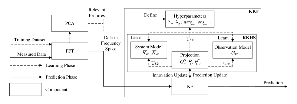
Figure 1: Overview of the FKKF

As mentioned in Section I, a traffic flow can be seen as a non-linear system with hidden states, unknown dynamics and high-dimensional observations in frequency domain. The Frequency-based Kernel Kalman Filter (FKKF)is tailored for prediction problems in non-linear systems with hidden states and high-dimensional observations in the frequency domain as suitable fine grained for flow prediction.

III-A Overview

The FKKF uses Kalman filtering as efficient inference technique for state estimation and further prediction [19]. However, as opposed to standard Kalman filtering, which only works in linear systems, the FKKF uses a hidden state representation that is embedded in a Reproducing Kernel Hilbert Space (RKHS). This space represents a non-linear transformation of the original state space into a possibly infinite dimensional kernel space. While the system and observation models for the systems of interest are typically non-linear in the original state space, they can be approximated efficiently in the RKHS by linear models [19]. Hence, standard Kalman filtering can be applied to this RKHS representation of the system. In addition the FKKF transforms its observations into the frequency domain in order to cope with the challenges of flow prediction.

Figure 1 gives an overview of our FKKF. It combines — and inherits from — several known techniques, which are KF, RKHS, Fast Fourier Transform (FFT), and PCA. The dashed lines show the learning phase, where relevant features are extracted from the training data set. After transforming the features into frequency space, a system model and observation model are learned. Several hyperparameters (see Table I) are defined to regularize the system and observation model, and to scale the bandwidth of the kernel function. The solid lines show the prediction phase where the measured data are also transformed into frequency space. These data are used for the innovation and prediction update of the Kalman filter. Since the system and observation model are linear in the RKHS, a projection between the RKHS and the original space is needed. This projection uses the learned models and defined parameters.

The FFT is a well known algorithm to transform a signal from the time domain into the frequency space [34]. For the flow prediction application, we have observed that prediction in frequency space is simpler than in the time domain as bursty traffic often looks arbitrary in time space but has a noticeable characteristic, which can be predicted, in the frequency space (see Figure 9). We use PCA to reduce the dimensionality of our observation space with a minimal amount of information loss [24]. We also use an extension of the KKF formulation called the sub-space KKF, which uses a sparse representation of the RKHS to facilitate computation on large data-sets. Next we give more details of our FKKF.

III-B Kernel based Kalman Filter

We assume to receive an observation $y_{t}$ from the system at time point $t$ whose true hidden state is denoted by $x_{t}$. We represent our belief over state $x_{t}$ with a mean embedding $\vec{\mu}_{\varphi(x_{t})}$ in a RKHS with the kernel $k(\vec{x}_{t},\vec{x}_{t+1})=\langle\vec{\varphi}(\vec{x}_{t}),\,\vec{\varphi}(\vec{x}_{t+1})\rangle$ and with a covariance embedding $\vec{\Sigma}_{\vec{\varphi}(\vec{x}_{t})}$ in a tensor-product RKHS with the kernel $h(\vec{x}_{t},\vec{x}_{t+1})=\langle\hat{\vec{\varphi}}(\vec{x}_{t}),\,\hat{\vec{\varphi}}(\vec{x}_{t+1})\rangle$, where $\hat{\vec{\varphi}}(\vec{x}_{t})=\vec{\varphi}(\vec{x}_{t})-\vec{\mu}_{\varphi(x_{t})}$ is the centered feature mapping. The mean embedding corresponds to the mean of the Gaussian belief distribution while the covariance embedding corresponds to the covariance in standard Kalman filtering. Moreover, the distribution over the observation $y_{t}$ is embedded into another RKHS. For easier distinction, this feature mapping is denoted by $\phi(y_{t})$. We write $\vec{\varphi}_{t}$ and $\vec{\varphi}_{t+1}$ instead of $\vec{\varphi}(\vec{x}_{t})$ and $\vec{\varphi}(\vec{x}_{t+1})$ respectively for simplicity.

The Kalman filter equations are composed of two updates – ($i$) the prediction update, which maps the current belief state to the next time step, and ($ii$) the innovation update, which incorporates the current observation in our belief state. As our system dynamics model as well as the observation model are unknown, both quantities need to be estimated from data. In the remainder of this section, we assume that we have access to a training data set, containng the state and observation trajectories, $\vec{x}_{1:T}$ to $\vec{y}_{1:T}$. The goal is to devise a state estimation and prediction algorithm that also works well on unseen test data.

Prediction update

We will start by embedding the prediction update in a RKHS. In Hilbert space, the mapping of the a posteriori mean embedding $\vec{\mu}_{\varphi_{t}}$ of time point $t$ to the prior mean embedding of the next state $\vec{\mu}_{\varphi_{t+1}}^{-}$ is given by a conditional operator $\mathcal{C}_{\varphi^{\prime}|\varphi}$. As our model is unknown, $\mathcal{C}_{\varphi^{\prime}|\varphi}$ needs to be computed using a sample-based estimator. This can be achieved as

$$\mathcal{C}_{\varphi^{\prime}|\varphi}=\vec{\Upsilon}_{x^{\prime}}\,(\vec{K}_{xx}+\lambda_{T}\vec{I}_{m})^{-1}\,\vec{\Upsilon}_{x}^{T},$$ (1)

where $\vec{K}_{xx}=\vec{\Upsilon}_{x}^{T}\,\vec{\Upsilon}_{x}$. The matrix $\vec{\Upsilon}_{x}=[\varphi(x_{1}),\,\dots,\,\varphi(x_{m}-1)]$ contains the feature mappings of all states and $\vec{\Upsilon}_{x^{\prime}}=[\varphi(x_{2}),\,\dots,\,\varphi(x_{m})]$ the mappings of all subsequent states. Therefore, the conditional operator is able to map the mean embeddings of the current state to the embedding of the next state. The parameter $\lambda_{T}$ is used to regularize the observation model (Gram matrix).The prediction update equations of the traditional KF can then be reformulated in a RKHS as

$$\vec{\mu}_{\varphi_{t+1}}^{-}=\mathcal{C}_{\varphi^{\prime}|\varphi}\,\vec{\mu}_{\varphi_{t}} \vec{\Sigma}_{\varphi_{t+1}}^{-}=\mathcal{C}_{\varphi^{\prime}|\varphi}\,\vec{\Sigma}_{\varphi_{t}}\,\mathcal{C}_{\varphi^{\prime}|\varphi}^{T}+\vec{\Upsilon}_{x^{\prime}}\,\vec{V}\,\vec{\Upsilon}_{x^{\prime}}^{T}$$ (2)

where $\vec{\Upsilon}_{x^{\prime}}\,\vec{V}\,\vec{\Upsilon}_{x^{\prime}}^{T}$ denotes the covariance of the zero-mean Gaussian noise of the transition model which is also learned from the training data set.

Innovation update

For the innovation update, we define an observation operator $\mathcal{C}_{\phi|\varphi}$ with $\phi(y_{t})=\mathcal{C}_{\phi|\varphi}\varphi(x_{t})+\nu$, where $\nu$ is zero-mean Gaussian noise. Thus, the operator maps the state embedding to the observation embedding and therefore, represents the FKKF equivalent of the observation matrix in the original KF formulation. The observation operator is estimated using the training data with $\mathcal{C}_{\phi|\varphi}=\vec{\Phi}_{y}\,(\vec{K}_{xx}+\lambda_{O}\vec{I_{m}})^{-1}\,\vec{\Upsilon}_{x}^{T}$, where $\vec{\Phi}_{y}=[\phi(y_{1}),\,\dots,\,\phi(y_{m})]$, and $\lambda_{O}$ is again a regularization parameter. In the original KF equations, the a priori mean and covariances are used in the innovation update together with the current observation $y_{t}$ to compute the Kalman gain, which represents the relative importance of the error with respect to the prior belief state estimation. Using the Kalman gain, we finally arrive at the a posteriori belief over the state. The Hilbert space equivalent of the innovation update equations are

$$\vec{\mu}_{\varphi_{t}}=\vec{\mu}_{\varphi_{t}}^{-}+\mathcal{Q}_{t}\,(\phi(y_{t})-\mathcal{C}_{\phi|\varphi}\,\vec{\mu}_{\varphi_{t}}^{-}) \vec{\Sigma}_{\varphi_{t}}=\vec{\Sigma}_{\varphi_{t}}^{-}-\mathcal{Q}_{t}\,\mathcal{C}_{\phi|\varphi}\,\vec{\Sigma}_{\varphi_{t}}^{-}$$ (3)

where the Kalman gain matrix is computed by

$$\mathcal{Q}_{t}=\vec{\Sigma}_{\varphi_{t}}^{-}\,\mathcal{C}_{\phi|\varphi}^{T}\,(\mathcal{C}_{\phi|\varphi}\,\vec{\Sigma}_{\varphi_{t}}^{-}\,\mathcal{C}_{\phi|\varphi}^{T}+\kappa\vec{I}_{m})^{-1}.$$ (4)

The zero-mean Gaussian noise of the observation model is estimated as $\kappa\vec{I}_{m}$.

State reconstruction

All computed means and covariances lie in the Hilbert space. Thus, an additional step is needed to map the embeddings back to the original state space. For this reconstruction of the state distribution another conditional operator $\mathcal{C}_{X|\varphi}$ is used. Similarly to the already defined conditional operators, it is computed using a sample-based estimator resulting in

$$\mathcal{C}_{X|\varphi}=\vec{X}\,(\vec{K}_{xx}+\lambda_{O}\vec{I}_{m})^{-1}\,\vec{\Upsilon}_{x}^{T}$$ (5)

with the hidden state matrix $\vec{X}=[x_{1},\,\dots,\,x_{m}]$. The reconstruction is now conducted by applying the conditional operator to the mean and covariance embeddings, yielding

$$\vec{\mu}_{x_{t}}=\mathcal{C}_{X|\varphi}\,\vec{\mu}_{\varphi_{t}} \vec{\Sigma}_{x_{t}}=\mathcal{C}_{X|\varphi}\,\vec{\Sigma}_{\varphi_{t}}\,\mathcal{C}_{X|\varphi}^{T}.$$ (6)

III-C Finite-sample RKHS Embedding

The FKKF embeds the state belief in a potentially infinite-dimensional Hilbert space using a non-linear feature map. In this high-dimensional space, non-linear inference can be performed by linear matrix operations as shown above.

As our models are unknown, $\mu_{\varphi_{t}}$ and $\Sigma_{\varphi_{t}}$ cannot be computed directly and need to be estimated. The estimation is done by representing the mean embedding at time point $t$ only by a finite vector $m_{t}\in\mathbb{R}^{m\times 1}$ and the covariance by a finite-dimensional matrix $\vec{S}_{t}\in\mathbb{R}^{m\times m}$ through

$$\vec{\mu}_{\varphi_{t}}=\vec{\Upsilon}_{x^{\prime}}\,m_{t} \vec{\Sigma}_{\varphi_{t}}=\vec{\Upsilon}_{x^{\prime}}\,\vec{S}_{t}\,\vec{\Upsilon}_{x^{\prime}}^{T}.$$ (7)

When inserted into the Equations 2, we receive a finite-sample prediction update formulation where the finite-dimensional a priori mean embedding is computed as

$$m_{t+1}^{-} =\vec{T}\,m_{t}.$$ (8)

The transition matrix $\vec{T}=(\vec{K}_{xx}+\lambda_{T}\vec{I}_{m})^{-1}\,\vec{K}_{xx^{\prime}}$ is the finite-dimensional equivalent to the conditional operator $\mathcal{C}_{\varphi^{\prime}|\varphi}$ and forms the learned model of the underlying system’s dynamics. For the covariance embedding estimation we receive

$$\vec{\Sigma}_{\varphi_{t+1}}^{-} =\mathcal{C}_{\varphi^{\prime}|\varphi}\,\vec{\Sigma}_{\varphi_{t}}\,\mathcal{C}_{\varphi^{\prime}|\varphi}^{T}+\vec{\Upsilon}_{x^{\prime}}\,\vec{V}\,\vec{\Upsilon}_{x^{\prime}}^{T}$$ (9)

$$\vec{S}_{t+1}^{-} =\vec{T}\,\vec{S}_{t}\,\vec{T}^{T}+\vec{V}.$$ (10)

As a next step, the equations for a finite-sample innovation update are introduced. The finite-dimensional Kalman gain matrix $\mathcal{Q}_{t}\in\mathbb{R}^{m\times m}$ is estimated by

$$\vec{Q}_{t}=\vec{S}_{t}^{-}\,\vec{O}^{T}\,(\vec{G}_{yy}\,\vec{O}\,\vec{S}_{t}^{-}\,\vec{O}^{T}+\kappa\,\vec{I}_{m})^{-1}$$ (11)

where $\vec{G}_{yy}=\vec{\Phi}_{y}^{T}\,\vec{\Phi}_{y}$ is the Gram matrix of the embedded observations. The learned observation model of the underlying system is given by $\vec{G}_{yy}\vec{O}$, where $\vec{O}=(\vec{K}_{xx}+\lambda_{O}\vec{I}_{m})^{-1}\,\vec{K}_{xx^{\prime}}$. The finite-dimensional Kalman gains can be extracted from the infinite-dimensional ones as $\mathcal{Q}_{t}=\vec{\Upsilon}_{x^{\prime}}\,\vec{Q}_{t}\vec{\Phi}_{y}^{T}$ . Using $\vec{Q}_{t}$, the finite-dimensional a posteriori mean embedding is derived as

$$m_{t} =m_{t}^{-}+\vec{Q}_{t}\,(k_{:y_{t}}-\vec{G}_{yy}\,\vec{O}\,m_{t}^{-}).$$ (12)

The observations are represented by the kernel vector $k_{:y_{t}}=[k(y_{1},y_{t}),\,\dots,\,k(y_{m},y_{t})]$. The finite-dimensional a posteriori covariance embedding is then calculated by

$$\mathcal{S}_{t} =\mathcal{S}_{t}^{-}-\vec{Q}_{t}\,\vec{G}_{yy}\,\vec{O}\,\mathcal{S}_{t}^{-}.$$ (13)

As for the infinite-dimensional case, the reconstruction of the state distribution is needed to map the mean and covariance embeddings back to the original space. For the mean and covariance, the derivations are

$$\vec{\mu}_{x_{t}}=\vec{X}\,\vec{O}\,m_{t} \vec{\Sigma}_{x_{t}}=\vec{X}\,\vec{O}\,\vec{S}_{t}\,\vec{O}^{T}\,\vec{X}^{T}.$$ (14)

III-D Sub-space FKKF

The Kernel Kalman Rule (KKR) possesses almost cubic computational complexity for the number of training samples due to the inversion of the Gram matrix $\vec{K}_{xx}\in\mathbb{R}^{m\times m}$ [19]. Thus, for large training sets the calculations become practically intractable. However, a sub-space FKKF variant can be defined that allows to work with large data sets. The core idea is to represent the mean embedding only by a subset of the training samples, while still all samples are used to learn the model. To achieve this, a sub-space feature mapping $\vec{\Gamma}_{x}=[\varphi(x_{1}),\,\dots,\,\varphi(x_{n-1})]$ which contains the mappings of only $n\ll m$ training samples is defined, such that $\vec{\Gamma}_{x}\subset\vec{\Upsilon}_{x}$. The Gram matrix is then calculated as $\vec{\overline{K}_{xx}}=\vec{\Upsilon}_{x}^{T}\,\vec{\Gamma}_{x}$ with dimensions $\vec{\overline{K}_{xx}}\in\mathbb{R}^{m\times n}$ leading to new conditional embedding operators for the model learning which are called sub-space conditional embedding operators, introduced in [19].

The formulations for the prediction update of the sub-space FKKF stay the same as for the full-space FKKF with

$$\vec{\mu_{\varphi_{t+1}}^{-}}=\mathcal{C}^{S}_{\varphi^{\prime}|\varphi}\,\vec{\mu_{\varphi_{t}}} \vec{\Sigma}_{\varphi_{t+1}}^{-}=\mathcal{C}^{S}_{\varphi^{\prime}|\varphi}\,\vec{\Sigma}_{\varphi_{t}}\,\mathcal{C}^{ST}_{\varphi^{\prime}|\varphi}+\vec{\Upsilon}_{x^{\prime}}\,\vec{V}\,\vec{\Upsilon}_{x^{\prime}}^{T}$$ (15)

but the conditional operator is now given by $\mathcal{C}^{S}_{\varphi^{\prime}|\varphi}=\vec{\Upsilon}_{x^{\prime}}\,\vec{\overline{K}}_{xx}\,\vec{L}_{T}^{S}\,\vec{\Gamma}_{x}^{T}$, where $\vec{L}_{T}^{S}=(\vec{\overline{K}}_{xx}^{T}\,\vec{\overline{K}}_{xx}+\lambda_{T}\vec{I}_{n})^{-1}$.
For the innovation update also the formulation of the the sub-space FKKF stay the same as for the full-space FKKF with the conditional operator mentioned before:

$$\vec{\mu}_{\varphi_{t}}=\vec{\mu}_{\varphi_{t}}^{-}+\mathcal{Q}^{S}_{t}\,(\phi(y_{t})-\mathcal{C}^{S}_{\phi|\varphi}\,\vec{\mu}_{\varphi_{t}}^{-}) \vec{\Sigma}_{\varphi_{t}}=\vec{\Sigma}_{\varphi_{t}}^{-}-\mathcal{Q}^{S}_{t}\,\mathcal{C}^{S}_{\phi|\varphi}\,\vec{\Sigma}_{\varphi_{t}}^{-}.$$ (16)

IV Putting the FKKF to Work

For the traffic prediction experiments described in Section V, we use the sub-space FKKF in order to make the computations tractable even when using a high number of training samples. This section presents our realization of the sub-space FKKF, shown as pseudocode in Algorithm 1, and its implementation on state of the art data center switching devices.

IV-A Preprocess Data

The main idea of preprocessing the data, is that the time series are seen as a time-discrete signal sampled using a sampling interval $T_{S}$. Instead of learning with the signal in the time domain we transform it to the frequency domain by making use of the Fourier Transform (FT). An advantage of conducting the calculations in the frequency domain is that since the FT is built over a part of the signal, much more information about the flow structure is contained in every data point which makes it easier to observe the current condition of the flow. Furthermore, since $T_{C}>T_{S}$ the data set will contain less data points in the frequency than in the time domain. This is especially useful when the training set consists of very long flows that would otherwise result in a large number of data points. The selection of an appropriate value for $T_{C}$ that leads to an overlap of the chunks also reduces artifacts in the frequency domain.

In the end, the resulting predictions are brought back to the time domain so that a TE system would receive them as kbit values which it could then use to compute optimal paths for the flows and reroute them accordingly. For representing the signal in the frequency domain, it first has to be split into smaller overlapping chunks of a certain length $w$. The starting points of the single chunks at which they are cut out of the original signal are defined by the sampling interval $T_{C}$. Consequently, the parameters $T_{S}$, $T_{C}$ and $w$ decide how many chunks the original signal is split into, and by how much the chunks overlap. Since the signal is discrete in time the Discrete Fourier Transform (DFT) needs to be used for the transformation and by splitting the signal in chunks, basically a discrete-time STFT is performed, whereas a FFT algorithm is used for making the FT computations faster (cf. [scale]).

IV-B Learning Phase

When using the sub-space FKKF for state estimation, the first step is to choose different settings for the execution of the algorithm. This includes choosing a training set $data_{train}$ and setting the values of multiple hyperparameters that are needed for the calculations and whose values are found through optimization in the learning phase. The hyperparameters $\lambda_{T}$ and $\lambda_{O}$ (see Eqs. 1 and 2 respectively) are used for regularizing the Gram matrix products before their inversion; the former parameter is used for the transition model during the prediction update step and the latter for the observation model during the innovation update step. The bandwidth scaling factors $state_{bw}$ and $obs_{bw}$ decide which values the bandwidths of the kernel functions — used for the state and observation embeddings — are multiplied with. The bandwidths are found by choosing a subset of training samples and calculating the median of the squared distances between them. The last hyperparameter is the observation noise covariance $\kappa$ (see Eq. 4). Besides forming a state representation out of observations, and thus allowing the FKKF to process data with a very high dimensionality, the preprocess-data function includes conducting a PCA on the training set. The PCA, which is conducted on a dataset after bringing it to the frequency domain and after standardizing it so that the set possesses zero mean and unit variance, reduces the dimensions needed for a single observation to lower their complexity and save computation time. The PCA uses an orthogonal transformation to compute principal components (PCs) corresponding to the dimensions of the dataset that are ordered in a descending order, meaning the first PC explains more variance of the dataset than any other PC. The assumption is that some frequencies might account for such a small amount of variance that their omission distorts the characteristics of the flow only insignificantly. It is important to mention that the PCA must always be conducted on the training set. The test set which is usually not fully available also needs to be standardized and its dimensionality reduced. However, for the transformation, the PCs computed from the training set must be used.

IV-C RKHS Embedding of the Kalman Filter

In the learn function the Gram matrices of the state embeddings denoted ${\overline{K}}_{xx}$ and ${\overline{K}}_{xx^{\prime}}$ (see Section III-D) are formed together with the observation Gram matrix ${G}_{yy}$. The matrices are then used to estimate the sub-space transition model matrix ${T}^{S}$ and the sub-space observation model matrix ${GO}^{S}$. Moreover, the state matrix ${X}$ needed for the projection back to the state space is formed and the initial values for the a priori sub-space mean embedding $\vec{n}_{1}^{-}$ and covariance embedding $\vec{P}_{1}^{-}$ are set.

Parameter	Description
$data_{train}$	Training set
$\lambda_{T}$	Regulation parameter for the transition model
$\lambda_{O}$	Regulation parameter for the observation model
$state_{bw}$	Scaling factors for the state embeddings
$obs_{bw}$	Scaling factors for the observation embeddings
$\kappa$	Observation noise covariance
${\overline{K}}_{xx}$, ${\overline{K}}_{xx^{\prime}}$	Gram matrices of the state embeddings
${G}_{yy}$	Observation Gram matrix
${T}^{S}$	Sub-space transition model matrix
${GO}^{S}$	Sub-space observation model matrix
${X}$	State matrix
${P}_{t}$	Covariance embedding
${Q}^{S}_{t}$	Sub-space Kalman gain matrix
${n}_{t}$	Sub-space mean embedding
$\mu_{x_{t}}$	Mean prediction
$\Sigma_{x_{t}}$	Covariance prediction

TABLE I: Parameters of the FKKF Algorithm

IV-D Prediction Phase

The FKKF algorithm can either be used online or offline. When used online, single observations would be omitted from the underlying system and directly used in the innovation update step. During the traffic prediction experiments described in Section V the algorithm was used offline. In the equations for the prediction and innovation updates shown in Section III, the Kalman gain matrices and the covariances were calculated together with the mean embeddings. However, none of the components depend on the current observation $y_{t}$ and therefore, they can be calculated before receiving any observation. Thus, the calculation can be done in the function project before testing the model which reduces the computation time needed for the FKKF algorithm (cf. [scale]). In the offline mode, the projection of ${Q}_{t}^{S}$, $P_{t}$ and $P_{t+1}^{-}$ allows to save computation time because when testing the model simultaneously with multiple test sets the components only have to be calculated once. The complexity of the prediction procedure has the complexity of a matrix-matrix multiplication with $O(n^{3})$ where $n$ here depends on the number of samples combined with the diversity of the flow structure, yet is independent of the number of flows and the number of network elements. There are also algorithms available with a lower complexity but the used algorithm is a block matrix algorithm where the blocks are small enough to fit into local memory which reduces the shifts into and out of memory.

In the last function the model is tested with given data, where the project function is called once before the prediction phase starts. The only step left in the predict function, for the innovation and prediction update, is the calculation of the a posteriori and the a priori sub-space mean embeddings $n_{t}$ and $n_{t+1}^{-}$, respectively. After the prediction, the mean and covariance embeddings are projected back into the state space. The prediction and innovation update steps can be executed alternately. However, if the observations arrive irregularly only every $p$-th time step, the algorithm will solely execute the prediction update step and thus perform a $p$-step prediction of the system state.

Algorithm 1 Core FKKF algorithm

function preprocess-data($data$)

     $stateWindow$ $\leftarrow$ form-state-windows($data$)

     $data$ $\leftarrow$ FFT($stateWindow$)

     return $data$

function learn($data_{train}$)

     while $data$ in $data_{train}$ do

         $data$ $\leftarrow$ preprocess-data($data$)

         $dimensionReducedData$ $\leftarrow$ pca($data$)

         $\langle\lambda_{T}$, $\lambda_{O}$, $state_{bw}$, $obs_{bw}$, $\kappa\rangle$ $\leftarrow$optimize-hyperparams ($dimensionReducedData$)

         $\langle\vec{T}^{S}$, $\vec{GO}^{S}$, $\vec{X}$, $\vec{n}_{1}^{-}$, $\vec{P}_{1}^{-}\rangle$ $\leftarrow$ estimate-model($\vec{\overline{K}}_{xx}$, $\vec{\overline{K}}_{xx^{{}^{\prime}}}$, $\vec{G}_{yy}$, $dimensionReducedData$)      

     return $\langle\lambda_{T}$, $\lambda_{O}$, $state_{bw}$, $obs_{bw}$, $\kappa$, $\vec{T}^{S}$, $\vec{GO}^{S}$, $\vec{X}$, $\vec{n}_{1}^{-}$, $\vec{P}_{1}^{-}$, $featureSet\rangle$

function project($learnedPara$)

     ${Q}_{t}^{S}$ $\leftarrow$ kalman-gain($learnedPara$)

     ${P}_{t}$ $\leftarrow$ a-posteriori-covariance-embed($learnedPara$)

     ${P}_{t+1}^{-}$ $\leftarrow$ a-priori-covariance-embed($learnedPara$)

     return $\langle{Q}_{t}^{S}$, ${P}_{t}$, ${P}_{t+1}^{-}\rangle$

function predict($data$, ${Q}_{t}^{S}$, ${P}_{t}$, ${P}_{t+1}^{-}$)

     $data$ $\leftarrow$ preprocess-data($data$)

     Innovation update:

     $\vec{n}_{t}$$\leftarrow$a-posteriori-mean-embedding($data$, ${Q}_{t}^{S}$, ${P}_{t}$, ${P}_{t+1}^{-}$)

     Prediction update:

     $\vec{n}_{t+1}^{-}$$\leftarrow$a-priori-mean-embedding ($data$, ${Q}_{t}^{S}$, ${P}_{t}$, ${P}_{t+1}^{-}$)

     Project into state space:

     $\vec{\mu}_{x_{t}}$$\leftarrow$mean-predict($data$, $n_{t}$, $n_{t+1}^{-}$, ${Q}_{t}^{S}$, ${P}_{t}$, ${P}_{t+1}^{-}$)

     $\vec{\Sigma}_{x_{t}}$$\leftarrow$covariance-predict($data$, $\vec{n}_{t}$, $\vec{n}_{t+1}^{-}$, ${Q}_{t}^{S}$, ${P}_{t}$, ${P}_{t+1}^{-}$)

     return $\langle\vec{\mu}_{x_{t}}$, $\vec{\Sigma}_{x_{t}}\rangle$

procedure test-model($data_{test}$)

     $\langle\vec{Q}_{t}^{S}$, $\vec{P}_{t}$, $\vec{P}_{t+1}^{-}\rangle$ $\leftarrow$ project($\lambda_{T}$, $\lambda_{O}$, $state_{bw}$, $obs_{bw}$, $\kappa$, $\vec{T}^{S}$, $\vec{GO}^{S}$, $\vec{X}$, $n_{1}^{-}$, $P_{1}^{-}$, $featureSet$)

     while $data$ in $data_{test}$ do

         $\langle\vec{\mu}_{x_{t}}$, $\vec{\Sigma}_{x_{t}}\rangle$ $\leftarrow$ predict($data$, ${Q}_{t}^{S}$, $\vec{P}_{t}$, $\vec{P}_{t+1}^{-}$)

         check-results ($\vec{\mu}_{x_{t}}$, $\vec{\Sigma}_{x_{t}}$, $data+1$)      

IV-E System Design

The requirements for fine grained prediction (cf. [nonlin]) lead to two immediate consequences when implementing prediction algorithms:

• The interval for fetching statistics of individual flows has to be small enough to allow the algorithm to learn the fine grained structure of a flow (in our case 10ms).

• The prediction and further steps have to be “close” to the forwarding plane to minimize latency. Predicting more in advance is likely to compromise on accuracy and so its more efficient to set the prediction time optimal with respect to accuracy, yet avoid additional latency between the signal, the prediction and further steps.

State of the art data center switching devices, as shown in Figure 2, have two main processing instances – ($i$) a management system (with a common CPU), and ($ii$) a forwarding Application Specific Integrated Circuit (ASIC). While the ASIC is optimized for fast packet forwarding, the management system communicates with other control plane instances (e.g., other switch management systems, Software-Defined Network controller) and updates the Ternary Content-Addressable Memory (TCAM) where the forwarding rules of the ASIC are maintained. Another task of the management system is to fetch statistics or packet samples from the ASIC. The ASIC provides statistics of all forwarding rules, of individual ports and aggregated statistics of the forwarding system.

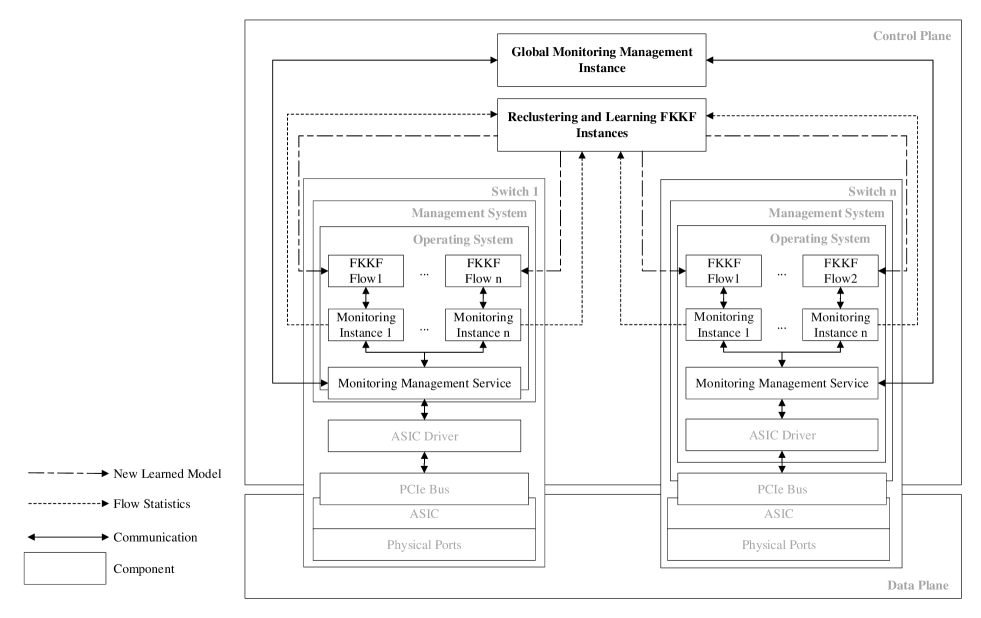
Figure 2: Overview of the FKKF system. The control plane summarizes the management systems of different switches, while the ASIC is responsible for fast packet forwarding as part of the data plane. A PCIe bus typically connects the ASIC and the management system where usually a Linux based OS is running with the communication interface (an ASIC driver) installed. This ASIC driver updates the TCAM and fetches the statistics from the ASIC. The monitoring system is implemented above the ASIC driver with its components (monitoring management service, monitoring instances) which communicate with a global monitoring management instance. The prediction algorithm runs on top of a monitoring instance and predicts the future traffic of individual flows. The monitoring instance sends a copy of the current statistics to a centralized reclustering and learning FKKF instance. This instance starts a new clustering and learning process if needed and submits the new model to the running FKKF instance.

Updating the TCAM, fetching the statistics, or receiving packet samples are done over a Peripheral Component Interconnect Express (PCIe) bus. On current white box switches, the management system typically runs a Linux-based operating system (OS). This OS can be open source (i.e. Open Network Linux (ONL) , OpenSwitch ) or extensible (i.e. Arista EOS). To be able to implement the FKKF, a new monitoring system had to be developed because existing approaches like sFlow [31] and IPFIX [14] are designed for fetching the data of interest from a switch and sending them to a centralized instance where they are analyzed. This process, even if all routes are globally optimized, takes too long because of the short prediction time as mentioned above. The new monitoring system now offers the possibility for complex processing of the monitored data directly on the switch. In short our monitoring system consists of ($a$) monitoring instances for each flow ($b$) one monitoring management service on each switch, and ($c$) a single global monitoring management instance (see Figure 2). The monitored data from the ASIC is forwarded over a monitoring management service which aggregates queries from different monitoring instances and sends the required data back to the monitoring instances. One of the mentioned individual monitoring instances can deliver the data to a FKKF instance to predict the trajectory of a given flow. The monitoring instances have their own state, which allows them to collect statistics, process them, and store data. The global monitoring instance forms a management system which communicates to the monitoring management services on the switches to synchronize and optimize the monitoring utilization. Note that the statistics from the monitoring instance is not only used for online prediction of the flow directly on switches, but also for offline classification and relearning of the flow structure (if needed, see IV-B). The prediction algorithm runs on the management system of the switch to receive the prediction as quickly as possible. Once the clustering and learning process is completed, the reclustering and learning FKKF instance updates the prediction model (described in IV) of the FKKF instance which is running on the switch. Such a system can now be used for new TE approaches as shown shortly in Section V.

V Evaluation

In this section we assess the performance of our FKKF in traffic flow prediction.

V-A Overview and Synopsis

To achieve the full potential of the FKKF, and configure its parameters, we have to understand the given data and their nature. Therefore, the nature of the data is first analyzed and explained (Section V-B). Then, the data is clustered into 20 different groups by calculating the Euclidean distance between the flows in the frequency domain. A subset of the contained flows is either selected for forming training or test sets (cf. [inter]), and processed by computing the FT and using the PCA to reduce data complexity of the data without loosing too much entropy (Section V-C). The trade-off between complexity and entropy of the data is optimized to run the FKKF algorithm on commodity switching hardware, as explained in Section IV-E, withouth increasing the prediction error (cf. [scale]). We evaluate both the prediction results and the run-time performance (Section V-D).Note that we predict the exact trajectory, which is much more sophisticated than probably needed for TE and congestion control mechanisms, where predicting the highest peak in the next prediction time frame suffices. By considering the highest peak, the prediction error of the FKKF, as well as of ARIMA and GARCH are calculated (see Table II). The run time performance measurements on commodity hardware switches shows how accurately the statistics can be polled and how many flows can be predicted on a switch.

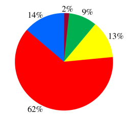
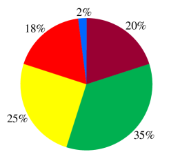
Figure 3: Characteristics of HTTP flows. Left duration of HTTP flows right Traffic load shares of duration groups

V-B Experimental Data

The data set used during the experiments was collected as part of a study conducted by Benson et al. that aimed at analyzing the characteristics of network traffic in data centers [8]. During their study, Simple Network Management Protocol (SNMP) data, topology information, and packet traces were collected from university data centers. Compared to other data sets (e.g., from Facebook) the chosen data set contains information up to the used application layer protocol type. We used the packet traces which contain 65 minutes worth of traffic data collected at an edge switch in a university data center consisting of 22 network devices and 500 servers.

In the first step, the packet traces were analyzed by gathering statistical information about the composition of the traffic data. For 87% of the traffic transmitted by the observed network switch, TCP was used as the transport layer protocol, and only 13% was transmitted over UDP. A closer look at the TCP traffic then revealed which protocols were used at the application layer. The Hypertext Transfer Protocol (HTTP) traffic makes up the largest share with 75% of the TCP traffic. Since the goal is to investigate if the progression of individual flows can be predicted, we focused on traffic using the same application layer protocol because we initially assumed that those flows would already share enough flow characteristics so that knowledge about some of the flows would allow us to predict other unseen ones. The decision was made in favor of HTTP traffic because this group contains 65% of all the collected traffic data.

However, further analysis of the HTTP traffic revealed that individual HTTP flows are very heterogeneous. The packet traces contain roughly 130 000 unique HTTP flows, where a flow represents a socket-to-socket connection between two hosts in the data center that starts with a TCP handshake and ends with a TCP teardown.

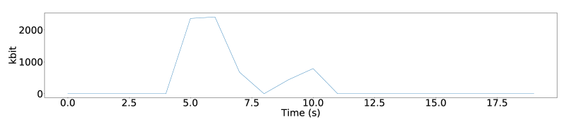
Figure 4: Sampling interval of 1s

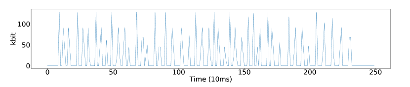
Figure 5: Fine grained flow structure of the first peak of the figure above with 10ms sampling size

As shown in Figure 3, the durations across HTTP flows are highly diverse. Most of the flows (62%) are very short with a length between 0.1s and 1s, as indicated by the red slice of the pie chart. To fully grasp the characteristics of HTTP flows it is important to know which share of the traffic load is caused by which duration group (group of flows with similar durations). This information is given in Figure 3 and together with Figure 3 yields interesting insights. The extremely short flows with a duration of up to 0.1s cause only 2% of the traffic and can therefore be neglected. The same goes for many flows in the duration group of 0.1s to 1s, though not for all of them. The most important group seems to be the one which contains flows with a rather short length between 1s and 100s, since only 22% of the flows possess such a length and still they cause 60% of the traffic. These traffic flows could not be captured when aggregating the flows as done in prior work as described in Section 1, since the flows would only be represented by one or a few data points (cf. [indiv]). Just the flows longer than 100s could be captured sufficiently (see Section V-D). As Figure 3 indicates, this duration group is responsible for 20% of the traffic. However, when examining the progression of high-volume long-lasting flows, a typical flow pattern is observed. One example flow is shown in Figure 4 which clearly reveals the extremely bursty nature of the network traffic. Even though an already rather low sampling interval of 1s is used, no flow structure can be observed since the short but very high peaks are only represented by one or two data points. For most of the time, the kbit values of the flow are either zero or are insignificant. This shows that even the long flows often just consist of short traffic peaks with long low-volume phases between them. For a TE system that tries to predict and reroute traffic in a network this means that it needs to be able to predict the flows on a small time scale because most of the traffic is transmitted in short high-volume traffic peaks. This also implies that the traffic data must be represented using a small sampling interval. Figure 5 shows the first peak of the same flow (Figure 4), however this time, a sampling interval of 0.01s was used and now much more information about the peak structure can be obtained.

As we can see, a peak itself consists of shorter peaks which we henceforth refer to as (peak) impulses. At the lowest possible sampling interval these impulses would represent single packets of the flows. In the vast majority of flows, the peaks consist of (1) a rising phase in which the peak impulses gradually increase up to a certain maximum kbit value and (2) a peak body where the traffic load remains rather constant. In the context of network congestion the rising phase is the most interesting part of the flow because here the traffic pattern of the flow is changing rapidly which causes congestion. Thus, the goal should be a successful prediction of the course of the peak rise given only a small part of it.

Therefore, we next investigate 603 single flows that transmit around 46% of all the HTTP traffic.

V-C Preprocessing the Data

As shown in Figure 6, the flow structure is extremely bursty when observed at a small sampling interval. As a consequence, the times series of kbit values produced from the flow packet traces contain many zero-value phases and generally high gradients. This makes the course of the time series difficult to learn for any model and is the reason why the approaches described in Section 1 aggregate the flows on a temporal scale and either is not applicable for linear time series with variable variance (ARIMA) and predict zeros or very low values, or start to oscillate arbitrarily (GARCH) because it can not predict the complex hidden state of the system. However, as we will see in Section V-D this would prevent a TE system from predicting short traffic peaks.

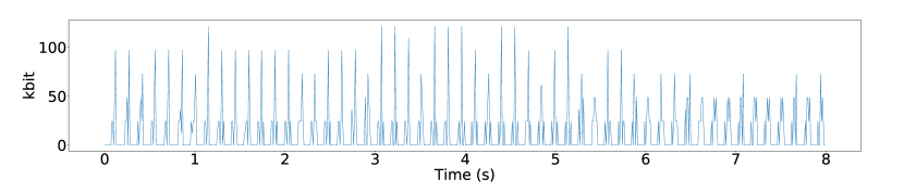
Figure 6: Traffic flows of recurring client-server communication

By learning the traffic signal in the frequency instead of the time domain the data sets that the KKF has to deal with become less bursty (see Section IV-A). Figure 9 compares the courses of different data series. In Figure 7 a 2s long flow chunk is shown. When computing the FT of the chunk, a data series as shown in Figure 8 is produced. The data series consists of complex numbers that describe the amplitudes and phases of simple sine waves that can be combined to construct the original signal. In the plot the amplitudes of the needed sine waves are shown. Furthermore, the plot reveals that the frequency values get folded at the Nyquist frequency $f_{N}$ which is half of the sampling frequency, $f_{N}=0.5\,f_{S}=0.5\,\frac{1}{T_{S}}$. For reconstructing the time signal from sine waves we therefore only need to save the first $N$ values of the FT results, with $N=f_{N}+1$. When transforming our results back to the time domain, the rest of the values can be reconstructed by inverting the imaginary parts of the saved complex numbers. However, in order to use the FT results with the FKKF, the complex numbers have to be split into their real and imaginary parts. The resulting data series consisting alternately of real and imaginary values is presented in Figure 9 which clearly shows that the data series is considerably less bursty than the original time series.

The influence of the transition to the frequency domain on the employed data set should now be illustrated using an example. We assume that the training set that the KKF should learn from consists of only one short high-volume flow with a duration of 10s. When using a sampling interval $T_{S}=0.01$ our training set $data_{train}$ contains a time series of kbit values observed every 0.01s and which possesses the dimensionality $data_{train}\in R^{1000x1}$. As mentioned in Section IV-A, the time signal is now split into single overlapping chunks. When using a sampling interval $T_{C}=0.05$ and a chunk length of $w=1$ the signal is split into 200 unique chunks that all contain 100 data points, where always 20 subsequent chunks overlap. In the next step, the FT is computed which returns a data series of 100 complex numbers for every chunk which represents a single observation in the frequency domain. As mentioned before, we only have to keep the first $N$ frequencies but need to split them into their real and imaginary parts which in the end leaves us with a series of 102 data points for every chunk. Altogether, our training set will now have the dimensionality $data_{train}\in R^{200x102}$. As we can see, the ability to work with the traffic data needs to be paid with an increase of the observation dimensionality.

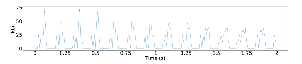
Figure 7: Signal chunk in the time domain

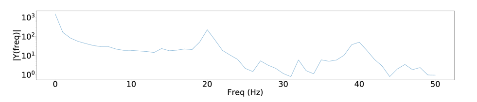
Figure 8: Signal chunk in the frequency domain

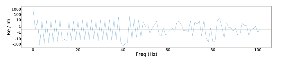
Figure 9: Signal chunk in the frequency domain with split complex numbers

As discussed in Section IV a PCA was used to reduce the complexity of the training data set and save computation time. The number of dimensions by which the data sets can be reduced with a PCA differs between the groups of recurrent flows. Figure 10 shows the cumulated explained variance over the principal components for two flow groups which represent the groups with the best and the worst cumulated explained variances respectively. As the plot reveals, fewer dimensions are needed for flow group 11 than for flow group 7 to explain the same amount of variance. The variance values were obtained by selecting all flows except one flow of each group as separate training sets and performing a PCA on them. The influence of the reduction on the flow structure in the time domain when reducing the dimensionality from 102 to 80 dimensions is acceptable. For flow group 7, a reduction of 20 dimensions leaves us with 89.9% of explained variance. The loss of information is still acceptable, even though it is clearly visible in the plot. For flow group 11, the remaining 80 dimensions are still enough to explain 99.8% of the variance. However, the plot demonstrates that for this flow group a larger percentage of information was contained in the omitted 20 dimensions since the heights of the flow peaks differ more from the original height. Therefore, the results match the insights already obtained from Figure 10. Considering also the results for other flow groups (see Table II column “PCA cum. expl. Variance (80 dim.)”), it has to be concluded that a PCA is useful for reducing the dimensionality of the utilized traffic data, a reduction of around 20 dimensions lead to a noteworthy reduction of complexity for further computation.

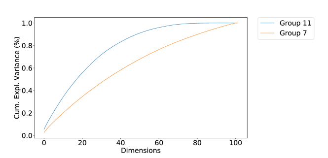
Figure 10: Comparison between lowest and highest cumulative explained variance per dimension

As mentioned in Section I, the training sets used during the experiments contain observations of kbit values which not represent the true (hidden) state of the underlying system. Our training sets only contain observations, however, as noted in Section IV-B, a window of observations can be used as an internal state representation. By computing the FT over chunks of the signal we are actually already building a window because the state is represented by the frequencies of a time signal chunk that consists of multiple observations. However, to extend the representation of the state during the prediction experiments, it was formed using the FTs of multiple chunks with increasing length. One possibility would e.g. be to use the FT of the next s and combine it with the FTs computed over the next 2 and 3s. This allows us to include some more long-term behavior of the flow in the state representation. In such a scenario, an observation would be represented by the FT over the next second of the time signal.

					prediction error
group ID	# flows	PCA cum. expl. Variance (80 dim.)	constant error	optimal chunk len.	chunk len. = 1s	chunk len. = optimal	ARIMA	GARCH
1	4	95.9%	-69.7%	0.15s	-43.1%	-2.0%	-96.3%	-97.9%
2	13	91.7%	-60.1%	0.4s	-36.3%	-8.4%	-100%	-98.6%
3	6	98.7%	-63.5%	0.55s	14.7%	5.6%	-100%	-96.6%
4	24	94.9%	-57.6%	0.2s	-62.3%	-22.8%	-99.9%	-98.2%
5	5	98.1%	-55.9%	0.2s	-53.1%	-12.1%	-91.8%	-95.5%
6	6	90.6%	-46.9%	0.15s	-52.8%	-13.2%	-97.7%	-97.5%
7	3	89.9%	-60.0%	0.25s	-4.5%	2.5%	-94.1%	-97.4%
8	10	97.0%	-79.6%	0.3s	-28.5%	-4.3%	-100%	-97.6%
9	4	99.5%	-66.7%	1.95s	-28.4%	-4.1%	-99.9%	-95.7%
10	4	98.5%	-63.2%	0.5s	-46.7%	-0.7%	-100%	-99.3%
11	5	99.8%	-54.3%	0.25s	-26.8%	-0.8%	-99.9%	-99.0%
12	18	95.9%	-60.4%	0.95s	-44.2%	-10.2%	-91.9%	4102.7%
13	5	94.3%	-45.5%	0.55s	-11.6%	-1.6%	-91.7%	98.7%
14	3	98.1%	-62.5%	0.35s	-63.8%	-10.2%	-99.7%	7490990.2%
15	11	90.6%	-52.2%	0.25s	-57.9%	-17.0%	-97.7%	-98.9%
16	13	93.2%	-37.5%	0.55s	-70.6%	-40.2%	-99.0%	-95.2%
17	3	91.4%	-26.4%	0.95s	-93.2%	-45.4%	-90.8%	-99.3%
18	4	98.6%	-35.7%	0.45s	151.9%	4.7%	-95.8%	13550.9%
19	7	93.4%	-70.0%	0.15s	-53.5%	-7.3%	-100%	603%
20	3	94.8%	-62.5%	0.95s	-53.7%	2.0%	-77.3%	1533.6%

TABLE II: Results of prediction experiments. While our FKKF achieves 10.9% prediction error in average over all flow groups, ARIMA and GARCH exhibit at best 77.3% and 95.2% prediction error respectively.

V-D Results

Finally, the traffic flows that originated from recurring connections are clustered in groups dependent on the characteristic in frequency space. In further traffic prediction experiments the clustered flow groups were used to test if the flow structure of single groups could be learned and used to predict unseen flows.

Prediction accuracy

20 groups with the highest numbers of flows were selected. The results are shown in Table II, where the column “# of flows” holds the information about how many flows each group contained. On average, one group consisted of 8 unique flows. The performance of the FKKF was tested on every flow group separately. During an experiment, always one flow was selected as the test set. The rest of the flows were used for constructing the training set (cf. [inter]). As noted previously, the data set representing a flow consists of a time series of kbit values. For the prediction experiments described in this section, a sampling interval $T_{S}=0.01$ was used for producing the data series and a chunk sampling interval of $T_{C}=0.05$ for splitting them into smaller chunks.

In Section V-B we showed the results of our traffic data analysis which revealed that HTTP traffic flows often consist of short traffic peaks that in turn can be divided into a rising phase and a phase with a mainly constant load level [10]. Therefore, the more important parts of the flows are the peak rises, which is why we explicitly concentrate our predictions on these parts. We tested the ability of the FKKF to predict the peak rises after only a few observations from the beginning of the peak. The number of observations differs between the flows and ranges between 3 and 60 steps in the frequency domain which corresponds to an observed time interval of 0.15s to 3s. When the observation stops and the true prediction begins, all flows still possess a low traffic load which then increases rapidly by around 150% on average during the next s. According to Benson et al.’s definition [10] all used traffic flows are unpredictable at the point of the last observation.

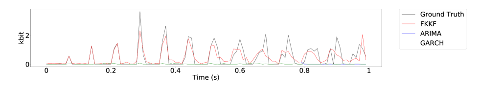
Figure 11: Comparison of FKKF, ARIMA and GARCH on flow group 3

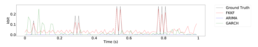
Figure 12: Comparison of FKKF, ARIMA and GARCH on flow group 19

The FKKF was always used for predicting a time period of 1s, resulting in 20 prediction steps in the frequency domain. The highest single impulse value predicted by the FKKF during this period was then compared to the actual highest impulse value in the same period. The difference between both values divided by the actual highest value represents the applied error metric for the prediction. The error should always be compared to the information that was already given in the observations. Therefore, another error metric was calculated for every flow group which helps to assess the quality of the prediction. In Table II the metric is shown in the “constant error” column. It was calculated like the prediction error only that the highest impulse value which emerged during the observation phase was used as the prediction, just as if we were predicting a constant load. Since we only observe the beginning of the peak rise, the picked impulse value will always be smaller than the actual one during the next s. Consequently, the actual value will always be underestimated which is why all values in the column are negative.

During the first set of experiments a chunk length $w=1$ was used for all flow groups. The internal state representation was then built by combining the FTs of the next s, the next 2s and the next 3s of the signal. An observation was represented by the FT of the next s. The prediction errors obtained for all flow groups are shown in column “chunk len. = 1s”. The performance of the FKKF for predicting a particular flow group is indicated by a red, yellow, or green coloring of the associated table cell which corresponds to a bad, moderate or good prediction performance respectively. Since it is difficult to assess the true prediction quality solely based on error metrics, a two-step approach was used.

In the first step, the computed prediction error and constant error values were utilized. Whenever the prediction error was above 50% or equally bad as the corresponding constant error value, the quality of the prediction was considered insufficient and the flow group marked in red. When the prediction error was lower than 50% and clearly smaller than the constant error, the group was marked in yellow. Only if a prediction error of less than 20% was achieved, the prediction was classified as good and marked in green. To illustrate the prediction results Figure 12 shows two prediction exemplary results of group 3 (Figure 11) and group 19 (Figure 12) for all considered approaches and the ground truth data. As expected, ARIMA and GARCH are not able to learn the hidden state of the system at every chunk length and consider the peaks as outliers (ARIMA) and predict zeros or very low values, or start to oscillate arbitrarily (GARCH) while the FKKF algorithm is able to predict the peaks accurately.

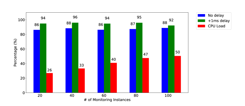
Figure 13: Accuracy and CPU load of the monitoring system with different number of monitoring instances and a polling interval of 10ms

Overhead

Being able to run our FKKF algorithm on commodity data center switch hardware is as important as achieving good prediction results. For the system evaluation we used a AS5512-54X  10G  switch from Edgecore with OpenSwitch. As discussed in Section IV-E the FKKF required a new monitoring system to poll the statistic of individual flows periodically at exact points in time because inaccurately measured data can highly influence the observed trajectory, leading to very inaccurate predictions. Therefore the developed monitoring system was optimized for accurate polling. Figure 13 shows the result of the monitoring polling accuracy with an interval of 10ms. On the $x$ axis different numbers of monitoring instances where tested. The blue bars show the accuracy without any delay. The green bars visualize the accuracy with 1ms delay which is still in an acceptable range. The red bars show the CPU load of one core with the given number of monitoring instances simultaneously. The tested switch has a quad core CPU for the management system, which means that by monitoring 100 individual flows only 50% of one core is occupied. As mentioned in Section IV-E the monitoring instance sends a copy of the monitored data to an instance which is responsible for reclassifying and relearning of a flow, if the prediction results of an individual flow are not accurate enough. This step is not time critical and can be computed on other devices with more computational resources (cf. [scale]). Therefore, it is not considered in the evaluation.

As shown in Figure 2 on top of the monitoring instances the FKKF instances are predicting a given flow. One FKKF prediction needs, on only one core, between 0.1ms and 10ms (on average 3.65ms) for running 1000 predictions in different flow groups. The variance is due to cache misses and context switches of the OS and computational optimization of the learned model. As shown in Table II the optimal chunk length varies between different flow groups. The average of optimal chunk length is 0.49s, which is the interval between two predictions. By taking the average processing time of the FKKF algorithm into account, more than 200 flows can be predicted on one switch (cf. [scale]).

VI Conclusions

In this paper we proposed an approach for predicting traffic flows focused on the short term prediction of peak structures of individual flows because, as shown during the analysis of real network traffic, this is the only type of prediction that truly considers the existing bursty nature of the network traffic that is a main cause of network congestion. In the conducted traffic prediction experiments, our FKKF was used to predict the peak rises in flow groups consisting of single flows from recurrent socket-to-socket connections, with observations only being given to the FKKF while the flows’ traffic load was still low. In 17 of the observed 20 groups, a prediction of the highest traffic impulse could be achieved with an average error of 6.43%.

Decentralized data processing (at the network devices) should also be considered in the development of any prospective TE system that aims at using prediction for rerouting network traffic. One idea is to realize several heterogeneous systemswhich will be simultaneously learning to optimize a global reward signal, e.g., to minimize the amount of network congestion for the given traffic profile. Due to the exploration actions of all agents, the global reward signal might be almost uncorrelated with the actions and observations of single agents. Therefore, the agents can combine the FKKF’s prediction with additional information from a global controller instance.

Our FKKF can be also used for mitigating other problems in the network than for dealing with congestion. Another interesting avenue for future research we are investigating is network security Here we are using our FKKF to learn and predict patterns of (distributed) denial-of-service attacks.

References

- [1] S. Agarwal, M. Kodialam, and T. V. Lakshman. Traffic Engineering in Software Defined Networks. INFOCOM, 2013, pages: 2211–2219.
- [2] M. Al-Fares, S. Radhakrishnan, B. Raghavan, N. Huang, and A. Vahdat. Hedera: Dynamic Flow Scheduling for Data Center Networks. NSDI, 2010, pages: 19–19.
- [3] M. Alizadeh, J. Crowcroft, L. Eggert, and K. Wehrle. Network Latency Control in Data Centres (Dagstuhl Seminar 16281). Dagstuhl Reports, 2016, pages: 15–30.
- [4] M. Alizadeh, A. Greenberg, D. Maltz, J. Padhye, P. Patel, B. Prabhakar, S. Sengupta, and M. Sridharan. Data center TCP (DCTCP). SIGCOMM, 2010, pages: 63–74.
- [5] N. C. Anand, C. Scoglio, and B. Natarajan. GARCH - Non-Linear Time Series Model for Traffic Modeling and Prediction. NOMS, 2008, pages: 694–697.
- [6] C. N. Babu and B. E. Reddy. Performance Comparison of Four New ARIMA-ANN Prediction Models on Internet Traffic Data. JTIT, 2015, pages: 67–75.
- [7] C. Benet, A. Kassler, E. Zola Predicting expected TCP throughput using genetic algorithm. Computer Networks 108, 2016, pages: 307–322.
- [8] T. Benson, A. Akella, and D. A. Maltz. Network Traffic Characteristics of Data Centers in the Wild. IMC, 2010, pages: 267–280.
- [9] T. Benson, A. Anand, A. Akella, and M. Zhang. Understanding Data Center Traffic Characteristics. SIGCOMM, 2010, pages: 92–99.
- [10] T. Benson, A. Anand, A. Akella, and M. Zhang. MicroTE: Fine Grained Traffic Engineering for Data Centers. CoNEXT, 2011, pages: 8:1–8:12.
- [11] S. Chabaa, A. Zeroual, and J. Antari. ANFIS Method for Forecasting Internet Traffic Time Series. MMS ”Mediterrannean Microwave Symposium”, 2009, pages: 1–4.
- [12] S. Chabaa, A. Zeroual, and J. Antari. Identification and Prediction of Internet Traffic Using Artificial Neural Networks. JILSA, 2010, pages: 147–155.
- [13] Y. Chen, B. Yang, and Q. Meng. Small-Time Scale Network Traffic Prediction Based on Flexible Neural Tree.
- [14] B. Claise. Specification of the IP Flow Information Export (IPFIX) Protocol for the Exchange of Flow Information. https://www.ietf.org/rfc/rfc7011.txt.
- [15] P. Cortez, M. Rio, M. Rocha, and P. Sousa. Internet Traffic Forecasting Using Neural Networks. IJCNN, 2006, pages: 2635–2642.
- [16] A. R. Curtis, W. Kim, and P. Yalagandula. Mahout: Low-Overhead Datacenter Traffic Management Using End-Host-Based Elephant Detection. INFOCOM, 2011, pages: 1629–1637.
- [17] M. Dong, Q. Li, D. Zarchy, P. B. Godfrey, M. Schapira. PCC: Re-architecting Congestion Control for Consistent High Performance. NSDI, 2015, pages: 395–408.
- [18] N. Dukkipati and N. McKeown. Why flowcompletion time is the right metric for congestion control and why this means we need new algorithms. ACM Computer Communication Review, 2006, pages: 59–62.
- [19] G. Gebhardt, A. Kupcsik, G. Neumann. The Kernel Kalman Rule - Efficient Nonparametric Inference with Recursive Least Squares. AAAI, 2017, pages: 3754–3760.
- [20] C. Hong, S. Kandula, R. Mahajan, M. Zhang, V. Gill, M. Nanduri, and R. Wattenhofer. Achieving High Utilization with Software-Driven WAN. SIGCOMM, 2013, pages: 15–26.
- [21] N. K. Hoong, P. K. Hoong, I. K. T. Tan, N. Muthuvelu, and L. C. Seng. Impact of Utilizing Forecasted Network Traffic for Data Transfers. ICACT, 2011, pages: 1199–1204.
- [22] P. K. Hoong, I. K. T. Tan, and C. Y. Keong. Bittorrent Network Traffic Forecasting with ARMA. CoRR, 2012, abs/1208.1896.
- [23] S. Jain, A. Kumar, S. Mandal, J. Ong, L. Poutievski, A. Singh, S. Venkata, J. Wanderer, J. Zhou, M. Zhu, J. Zolla, U. Hölzle, S. Stuart, and A. Vahdat. B4: Experience with a Globally-Deployed Software Defined WAN. SIGCOMM, 2013, pages: 3–14.
- [24] I. Jolliffe. Principal Component Analysis. Wiley Online Library, 2002.
- [25] L. Jose, L. Yan, M. Alizadeh, G. Varghese, N. McKeown, and S. Katti. High Speed Networks Need Proactive Congestion Control. HotNets, 2015, pages: 14:1–14:7.
- [26] D. Katabi, M. Handley, and C. Rohrs. Congestion control for high bandwidth-delay product networks. SIGCOMM, 2002, pages: 89–102.
- [27] C. Katris, S. Daskalaki. Comparing forecasting approaches for Internet traffic. Expert Systems with Applications, 2015, pages: 8172–8183.
- [28] Y. Liang and L. Qiu. Network Traffic Prediction Based on SVR Improved by Chaos Theory and Ant Colony Optimization. IJFGCN, 2015, pages: 69–78.
- [29] K. Papagiannaki, N. Taft, S. Bhattacharyya, P. Thiran, K. Salamatian, and C. Diot A pragmatic definition of elephants in internet backbone traffic. SIGCOMM Workshop on Internet measurment, 2002, pages: 175–176.
- [30] D. C. Park and D. M. Woo. Prediction of Network Traffic Using Dynamic Bilinear Recurrent Neural Network. ICNC, 2009, pages: 419–423.
- [31] P. Phaal. InMon Corporation’s sFlow: A Method for Monitoring Traffic in Switched and Routed Networks. https://www.ietf.org/rfc/rfc3176.txt.
- [32] L. Ralaivola and F. d’Alche Buc. Time Series Filtering, Smoothing and Learning Using the Kernel Kalman Filter. IJCNN, 2005, pages: 1449–1454.
- [33] B. Vujicic, H. Chen, and L. Trajkovic. Prediction of Traffic in a Public Safety Network. ISCAS, 2006, pages: 4 pp.–.
- [34] P. Welch. The Use of Fast Fourier Transform for the Estimation of Power Spectra: a Method Based on Time Averaging over Short, Modified Periodograms. IEEE Transactions on audio and electroacoustics, 1967, 15(2):70–73.
- [35] Y. Yu, M. Song, Y. Fu, and J. Song. Traffic Prediction in 3g Mobile Networks Based on Multifractal Exploration. Tsinghua Science and Technology, 2013, 18(4):398–405.
- [36] P. Zhu, B. Chen, and J. C. Prı´ncipe. Learning Nonlinear Generative Models of Time Series with a Kalman Filter in RKHS. IEEE Transactions on Signal Processing, 2014, 62(1):141–155.