The problem of the height dependence of magnetic fields in sunspots
keywords:
Sunspots, Magnetic Fields, Umbra, Penumbra, Photosphere, Chromosphere1 Introduction
s:intro
More than hundred years ago, it was proven that sunspots are concentrations of strong magnetic fields with a central field strength of 3000 G and more (Hale, 1908). Sunspots exist for several days or even weeks, and after the formation process, they often exhibit a stable appearance before they finally decay. This means, sunspots are in hydrostatic equilibrium with their surroundings which are stratified by the gas pressure. The magnetic field in the sunspots causes another pressure term reducing the inner gas pressure. Hydrostatic equilibrium then requires that the magnetic field strength is height dependent and decreases with height. Many attempts were carried out to determine this height dependence, but up to now, various methods led to different height gradients. Observations based on different spectral lines originating in different atmospheric layers yield a steep gradient of the magnetic field with height ( to G km-1), while investigations under the divergence-free assumption yield shallower gradients ( G km-1). Gradients between 0 and G km-1 are considered as shallow and gradients beyond G km-1 as steep. Negative values for these gradients indicate a decrease with height, and this convention will be kept throughout this review, although some authors follow the opposite convention. Furthermore, I shall give all gradients in [ G km-1], however, it is clear that such values are only valid for a narrow height range. The discrepancy between the methods was discussed before by Solanki (2003) in his review on sunspots, and he states that no satisfactory solution was found for the small gradients in the second case. Nevertheless, it may be as well that the large gradients based on different spectral lines do not reflect the real situation on the Sun. So far, it is still an open question what causes these differences.
It is the main aim of this article to give an overview about the existing observations and to discuss possible problems of the applied methods, and which ideas have been followed to explain the discrepancy. Section \irefS:deltaB provides an overview about previous works based on spectral lines and their profiles, and in Section \irefS:divB investigations based on div are presented. Gradients in pores are summarized in Section \irefS:pores. Coronal observations at radio wavelengths are considered in Section \irefS:radio. Indirect methods based on the magnetic flux and the pressure balance are presented in Sections \irefS:flux and \irefS:p_balance. Numerical simulations are the topic of Section \irefS:numsim. Finally, in the discussion (Section \irefS:discussion), I consider several other possibilities that have been proposed to explain the discrepancy between the methods, although none of these explanations is a convincing solution for the problem.
2 Observations based on different spectral lines and line profiles
S:deltaB
Spectral lines are formed in a certain range of the solar atmosphere. Depending on temperature, the abundance of the ion and the parameters of the atomic transition, this range can be quite narrow or rather extended. In general, strong lines cover a wider range of the atmosphere and deliver information about higher layers. Weak lines are formed in a narrow range which is normally located in the lower atmosphere. Observing several lines simultaneously allows us to probe different heights of the solar atmosphere. In the classical way, different lines are investigated separately, and the magnetic gradient is calculated from the differences according to Equation \irefEq_def_grad.
| (1) |
Nowadays, modern inversion techniques allow us also to evaluate several spectral lines simultaneously and obtain the magnetic gradient making use of the coverage of a wide height range.
2.1 Height dependence of the total and longitudinal magnetic field strength
In this first step, publications where the height dependence of the total magnetic field strength or its longitudinal component was determined, are considered. The results are valid for the umbra if nothing else is explicitly mentioned. Wittmann (1974) investigated the spectral lines Fe i 525.02 nm, Fe i 617.34 nm, Fe i 621.34 nm, Fe i 630.25 nm, Fe i 633.68 nm, and V i 625.69 nm obtained from spectro-polarimetric observations. He found a gradient of the magnetic field strength of G km-1. Pahlke and Wiehr (1990) recorded many spectral lines in the range 611 – 618 nm simultaneously in circular polarization. They used a combination of two different model atmospheres, a hot and a cool one, and created diagnostic diagrams for the spectral lines. The best fit was obtained for a gradient of G km-1. An even steeper gradient of to G km-1 was found by Balthasar and Schmidt (1993) from the superposed pattern of the Zeeman components of three different iron lines Fe ii 614.9 nm, Fe i 630.25 nm and Fe i 684.2 nm. For this purpose, they compared the observed line profiles with a set of calculated ones and selected that with the highest correlation coefficient.
In the last decade of the twentieth century, spectro-polarimetric inversion codes came up, and sophisticated polarimeters were built. To determine the magnetic gradient, there are two options. Such inversion codes use stratified atmospheres and are thus able to determine height dependencies from different parts of the Stokes-profiles, even from a single line. The full calculation for all atmospheric layers is time-consuming. To save computing time, many codes perform the full calculation only for a small number of atmospheric levels (“nodes”) and interpolate for the levels between the nodes. However, one has to be careful that gradients determined this way are realistic. Depending on where the nodes are placed, it might happen that layers with low contribution to the line profile influence the result and lead to unrealistic inverse gradients or “ringing” effects. The other option is to invert profiles from two or more spectral lines originating in different atmospheric layers independently, but assuming the magnetic parameters are height independent. The magnetic field strength is different for the individual lines, and from this difference divided by the height difference, the magnetic gradient is determined, as described in Equation \irefEq_def_grad. Both methods yield similar gradients, as shown in the following.
Collados et al. (1994) used data obtained at the Gregory-Coudé-Telescope (GCT) in Tenerife and applied the Stokes Inversion based on Response functions (SIR) code (Ruiz Cobo and del Toro Iniesta, 1992) to create model atmospheres for different sunspots. The spectral lines Fe i 629.8 nm, Fe i 630.15 nm and Fe i 630.25 nm were inverted together height-dependently for the magnetic field. For the mid photosphere they found a gradient of G km-1 for a small “hot” sunspot (with an umbral temperature of 5030 K at lg ) and G km-1 for a large cool one (T = 3940 K). They found indications that the gradients become steeper and more similar for different spots in deep layers of the atmosphere. Westendorp Plaza et al. (2001) analyzed data obtained at the Dunn Solar Telescope, (DST, Dunn, 1969) also with the SIR code, and from the two lines Fe i 630.15 nm and Fe i 630.25 nm they found a gradient of to G km-1. A similar gradient was found by Sánchez Cuberes, Puschmann, and Wiehr (2005) from a pair of near infrared lines, Fe i 1078.3 nm and Si i 1078.6 nm observed at the Vacuum Tower Telescope (VTT, von der Lühe, 1998) with the Tenerife Infrared Polarimeter (TIP, Collados et al., 2007). They also used the SIR-code and performed an inversion with a height dependent magnetic field for both lines together. Mathew et al. (2003) observed also with TIP at the VTT and used the Stokes-Profile-INversion-O-Routines code (SPINOR, Frutiger et al., 2000). They obtained even G km-1 from the lines Fe i 1564.8 nm and Fe i 1565.2 nm which probe the deepest layers of the photosphere, together with two OH molecular lines recorded in the same spectral range. The molecular lines originate in the upper photosphere. In their inversion, they used six nodes at fixed optical depths for the height dependence of the magnetic field.
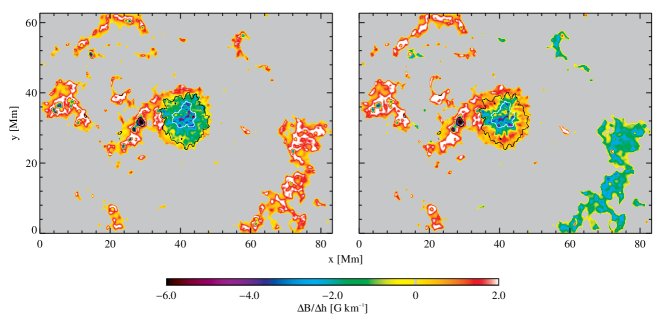
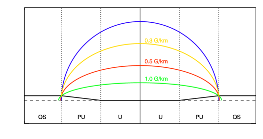
Balthasar and Gömöry (2008) observed a small sunspot with TIP at the VTT and used the same spectral lines as Sánchez Cuberes, Puschmann, and Wiehr (2005). Both lines are Zeeman triplets with a splitting factor of 1.5, but they differ in the formation height. The silicon line originates higher, except for cool umbrae. The two lines were recorded strictly simultaneously. Because of the small distance of only 0.3 nm, they fit on the same detector. Inversions with the SIR-code were performed independently for the two lines, but without height dependence of the single lines. In the umbra, they found an average gradient of G km-1 and in the penumbra a range of to G km-1. The increase of the magnetic field outside the penumbra is explained by the magnetic canopy. The gradient varies significantly within the umbra indicating an internal structure of the umbra (see Figure \ireffig:BandG_bbh).
Observations with two telescopes at the Observatorio del Teide, Tenerife, were combined by Balthasar and Bommier (2009). They observed at the VTT the same lines as (Balthasar and Gömöry, 2008) and Fe i 630.15 nm, Fe i 630.25 nm and Cr i 578.2 nm at the Télescope Héliographique pour l’Etude du Magnetisme et des Instabilités Solaires (THEMIS, Gelly, 2007) and applied the SIR-code. They found a gradient of the magnetic field strength of up to G km-1 in the umbra and G km-1 for the inner penumbra.
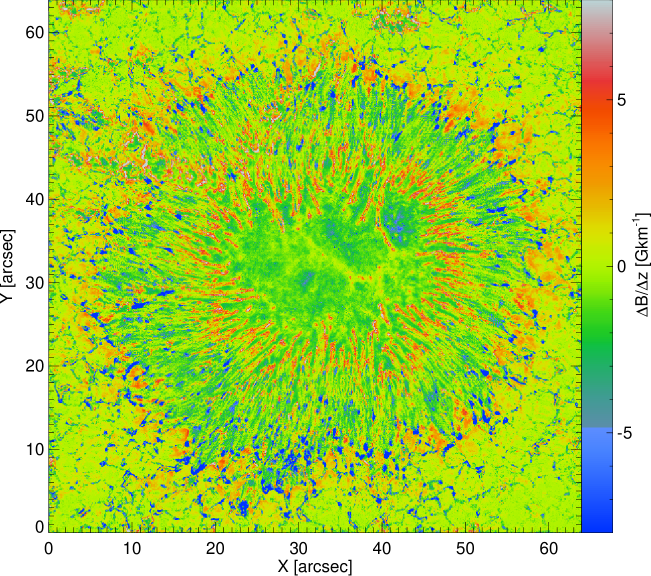
Bommier (2013) also used THEMIS and recorded full-Stokes spectra of the lines Fe i 630.15 nm and Fe i 630.25 nm. She inverted the line profiles separately with the UNNOFIT-code (Bommier et al., 2007) and found to G km-1 for the vertical gradient of the magnetic field. Balthasar et al. (2014a) observed the same lines as Balthasar and Gömöry (2008), inverted them with the SIR-code and obtained a gradient of G km-1 for the main umbra of a -spot (-spots harbor umbrae of both magnetic polarities within the same penumbra) and G km-1in the -umbra. Tiwari et al. (2015) investigated data with the same spectral lines from the Japanese Hinode spacecraft (Kosugi et al., 2007) taken with the SOT spectropolarimeter (Tsuneta et al., 2008; Ichimoto et al., 2008). As Mathew et al. (2003), they used the SPINOR-code for the inversion. In the umbra, they found a gradient of the total magnetic field strength of G km-1. In the penumbra, they obtained a very structured distribution, and in certain locations of the inner penumbra, they even found positive gradients, as shown in Figure \ireffig:tiwari8. Joshi et al. (2017b) confirmed such positive gradients for the inner penumbra from photospheric lines recorded in the near infrared at the VTT and inverted with SPINOR.
Felipe et al. (2016) found a decrease for the outer (faint) umbra from observations with the GREGOR solar telescope (Schmidt et al., 2012) and SIR-inversions. For the central umbra and for the penumbra they found very small gradients. The spot investigated by them exhibited a light bridge (LB) with a small magnetic field strength at low photospheric level increasing almost to the field strength of the faint umbra at lg = . Comparably small gradients of about G km-1 for the umbra are reported by Verma et al. (2018), who used the spectral lines Si i 1082.7 nm and Ca i 1083.9 nm observed at the GREGOR telescope. The same authors determined G km-1 for the normal penumbra. This spot exhibited an elongated umbral core (EUC) embedded in an irregular part of the penumbra, and here the gradient was G km-1.
Very sensitive to the magnetic field is the magnesium line at 12.32 m, because the sensitivity scales with the wavelength. On the other hand, the spatial resolution decreases, and more efforts (cooling) are needed to operate detectors for such wavelengths. Therefore, only a few attempts have been undertaken to used this line to determine the height dependence of the magnetic field. Bruls et al. (1995) compared a series of synthetic line profile with observations of Hewagama et al. (1993) at the McMath-Pierce telescope (Pierce, 1964) at the Kitt Peak Observatory and found a range of to G km-1 for the gradient in penumbrae, the steeper values occur close to the umbra. Moran et al. (2000) compared this line with Fe i 1564.8 nm with Fe i 1564.8 nm and reported a gradient of G km-1 for the umbra and G km-1 for the penumbra.
| Author | spectral lines | umbra | penumbra |
|---|---|---|---|
| Wittmann (1974) | several lines | G km-1 | |
| Pahlke and Wiehr | several lines | G km-1 | |
| (1990) | |||
| Balthasar and | Fe i 684.2 nm | – G km-1 | |
| Schmidt (1993) | Fe i 630.25 nm | ||
| Fe ii 614.9 nm | |||
| Collados et al. (1994) | Fe i 629.78 nm | G km-1 | |
| Fe i 630.15 nm | G km-1(dark U) | ||
| Fe i 630.25 nm | |||
| Bruls et al. (1995) | Mg i 12.32 m | – G km-1 | |
| Moran et al. (2000) | Mg i 12.32 m | G km-1 | G km-1 |
| Fe i 1564.8 nm | |||
| Westendorp Plaza | Fe i 630.15 nm | – G km-1 | |
| et al. (2001) | Fe i 630.25 nm | ||
| Mathew et al. (2003) | Fe i 1564.8 nm | G km-1 | |
| Fe i 1565.2 nm | |||
| OH 1565.19 nm | |||
| OH 1565.35 nm | |||
| Sánchez Cuberes | Fe i 1078.3 nm | ||
| et al. (2005) | Si i 1078.6 nm | ||
| Balthasar and | Fe i 1078.3 nm | G km-1 | – G km-1 |
| Gömöry (2008) | Si i 1078.6 nm | ||
| Balthasar and | several lines | G km-1 | G km-1 |
| Bommier (2009) | |||
| Bommier (2013) | Fe i 630.15 nm | – G km-1 | |
| Fe i 630.25 nm | |||
| Balthasar et al. | Fe i 1078.3 nm | G km-1 | |
| (2014a) | Si i 1078.6 nm | G km-1(-U) | |
| Tiwari et al. (2015) | Fe i 630.15 nm | G km-1 | outer PU |
| Fe i 630.25 nm | G km-1 | inner PU | |
| Felipe et al. (2016) | Si i 1082.7 nm | ||
| Ca i 1083.9 nm | (LB) | ||
| Joshi et al. (2017a) | Si i 1082.7 nm | inner PU | |
| Ca i 1083.3 nm | |||
| Verma et al. (2018) | Si i 1082.7 nm | G km-1 | G km-1 |
| Ca i 1083.9 nm | G km-1(EUC) |
All spectral lines discussed so far originate in the photosphere. In general it is more difficult to determine the magnetic field strength from chromospheric lines. There is only a limited selection of spectral lines coming from the chromosphere, most of them belong to light and abundant ions, thus the components of the line profiles are broader. Local thermal equilibrium (LTE) is no longer valid for these lines, and a proper inversion requires more efforts than for photospheric lines. In addition, most of these lines are not Zeeman triplets, and their effective Landé factor is two or even less. Nevertheless, chromospheric lines have been used to determine chromospheric magnetic fields, but often only with approximations to estimate the magnetic field. Results obtained in combination with photospheric lines obtained by Abdussamatov (1971), Rüedi, Solanki, and Livingston (1995), Liu et al. (1996), Orozco Suárez, Lagg, and Solanki (2005), Berlicki, Mein, and Schmieder (2006), Schad et al. (2015), Joshi et al. (2016), and Joshi et al. (2017a) are summarized in Table \ireftbl:chrom. Abdussamatov (1971) recorded the spectral lines H, Na D1 and D2 and Fe i 630.25 nm on photographic plates and found gradients G km-1 for strong magnetic fields ( G) and G km-1 for weaker fields. Rüedi, Solanki, and Livingston (1995) measured the circular polarization of the helium lines around 1083 nm with the main spectrograph of the McMath-Pierce telescope and compared them with observations in the line Fe i 1089.6 nm with the Fourier-Transform-Spectrometer. They determined gradients between and G km-1 for the umbra and shallower gradients for the penumbra. Liu et al. (1996) observed the H line and Fe i 532.4 nm with the Solar Magnetic Field Telescope at the Huairou Solar Observing Station, where they obtained photospheric vector magnetograms and chromospheric longitudinal magnetograms. They determined a range of to G km-1 for the magnetic gradient from the difference method. Orozco Suárez, Lagg, and Solanki (2005) performed simultaneous observations at the VTT with TIP in the lines He i 1083 nm and Si i 1082.7 nm. They inverted the silicon line with SPINOR and the helium line with the HeLIx-code (Lagg et al., 2004). Assuming a height difference of 2000 km between the two lines, they found gradients between and G km-1. Berlicki, Mein, and Schmieder (2006) measured the line-of-sight (LOS)-component of the magnetic field at THEMIS and obtained a relative gradient of km-1. Depending on the reference value, this amounts to to G km-1. Schad et al. (2015) used the Facility Infrared Spectropolarimeter (FIRS, Jaeggli et al., 2010) at the DST to record the helium and the silicon line at 1083 nm. Their result of G km-1 is in the same order as comparable investigations. Joshi et al. (2017a) observed with TIP at the VTT and found also values between and G km-1.
| Author | spectral lines | umbra | penumbra |
|---|---|---|---|
| Abdussamatov (1971) | H | – G km-1 | |
| Na D1 | |||
| Fe i 630.25 nm | |||
| Henze et al. (1982) | C iv 154.6 nm | – G km-1 | |
| Fe i 525.0 nm | |||
| Hagyard et al. (1983) | C iv 154.6 nm | G km-1 | |
| Fe i 525.0 nm | |||
| Rüedi et al. (1995) | He i 1083.0 nm | – G km-1 | – G km-1 |
| Fe i 1089.6 nm | |||
| Fe i 1078.3 nm | |||
| Liu et al. (1996) | H | – G km-1 | |
| Fe i 532.42 nm | |||
| Orozco Suárez et al. | He i 1083.0 nm | – G km-1 | |
| (2005) | Si i 1082.7 nm | ||
| Berlicki et al. (2006) | Na D1 | – G km-1 | |
| Ni i 676.8 nm | |||
| Schad et al. (2015) | He i 1083.0 nm | G km-1 | |
| Si i 1082.7 nm | |||
| Joshi et al. (2016) | He i 1083.0 nm | G km-1 inner PU | |
| Si i 1082.7 nm | G km-1 outer PU | ||
| Joshi et al. (2017a) | He i 1083.0 nm | – G km-1 | – G km-1 |
| Si i 1082.7 nm | outer to inner PU | ||
| Ca i 1083.3 nm |
Henze et al. (1982) and Hagyard et al. (1983) combined ground based observations with space based recordings of a C iv line at 154.8 nm with the Ultraviolet Spectrometer and Polarimeter (UVSP, Woodgate et al., 1980) on board the Solar Maximum mission. Their results are also listed in Table \ireftbl:chrom, but they do not differ significantly from only ground based observations. All these values are smaller than those from investigations where only photospheric lines were used. The height difference is 1000 km or more, while it is of the order of 100 – 200 km in the photospheric case. For the penumbra, the gradients are somewhat shallower than for the umbra, especially in the outer penumbra. A recent example is given by Joshi et al. (2016), who used GRIS at GREGOR to record the lines He i 1083.0 nm and Si i 1082.7 nm.
2.2 Height dependence of the vertical component of the magnetic field
If the full Stokes vector is measured, and the polarimetric azimuth ambiguity is solved, it becomes possible to investigate the height dependence of the vertical component of the magnetic field . Here one has to keep in mind that the sign of can be negative in contrast to the total field strength. Then a decrease of the total field strength coincides with a positive gradient of the vertical magnetic component. In the following, I ignore the sign of and show a negative gradient when the absolute values of the vertical component of the magnetic field strength decreases with height. However, the absolute value of the vertical component may increase with height, which is often the case in the outer penumbra. Results of such investigations are listed in Table \ireftbl:b_z. Some of these results are based on the same data sets discussed already in the previous section.
| Authors | spectral lines | umbra | penumbra |
|---|---|---|---|
| Eibe et al. (2002) | Na D1 | – G km-1 | |
| Balthasar and Gömöry | Fe i 1078.3 nm | G km-1 | 1–2 G km-1 |
| (2008) (VTT) | Si i 1078.6 nm | (outer PU) | |
| Balthasar et al. (2013) | Fe i 1078.3 nm | – G km-1 | |
| (VTT) | Si i 1078.6 nm | ||
| (Hinode) | Fe i 630.15 nm | – G km-1 | |
| Fe i 630.25 nm | |||
| Bommier (2013) | Fe i 630.15 nm | – G km-1 | |
| (THEMIS) | Fe i 630.25 nm | ||
| Balthasar et al. (2014b) | Fe i 1078.3 nm | – G km-1 | |
| (VTT) | Si i 1078.6 nm | G km-1(-um.) | |
| Jaeggli et al. (2012) | Fe i 630.2 nm | 0 – G km-1 | – G km-1 |
| Fe i 1565. nm | |||
| Verma et al. (2018) | Ca i 1083.9 nm | G km-1 | G km-1 |
| (GREGOR GRIS) | Si i 1078.6 nm | G km-1(EUC) |
The results of Balthasar and Gömöry (2008) are displayed in the right panel of Figure \ireffig:BandG_bbh. Similar values were obtained by Balthasar et al. (2013). Bommier (2013) found steep gradients from THEMIS observations. For the special case of a -spot, Balthasar et al. (2014b) also found steep gradients, especially for the -umbra. Eibe et al. (2002) investigated the LOS-component of the magnetic field determined from the Na D1 line. The sunspot observed by them was located about 20∘ off the disk center, thus the LOS-component is an approximation for the vertical component of the magnetic field. They determined the decrease relative to the value of the measured field strength and obtain 1. km-1. They measured field strengths up to 1000 G, and with these values, one gets the values given in Table \ireftbl:b_z. This investigation of Eibe et al. (2002) is the only one considering a single chromospheric line listed in Table \ireftbl:b_z. Therefore the values are clearly lower than the others, where also photospheric lines were included. While the investigation of Jaeggli et al. (2012) shows a wide variation from to G km-1, Verma et al. (2018) found shallower gradients around G km-1. Jaeggli et al. (2012) compared simultaneous observations with the FIRS at the DST of the lines Fe i 1565 nm and Fe i 630.25 nm, and inverted them with the Milne-Eddington code Two-Component-Magneto-Optical code (2CMO) based on a formalism of Jefferies, Lites, and Skumnaich (1989).
Summarizing, in the umbra, similar gradients are found as for the total magnetic field strength. They are slightly shallower since the absolute value of in general is smaller than the total field strength. In the outer penumbra, the opposite sign is found in several cases. The magnetic field in deep layers is almost horizontal. Thus the vertical component is very small and increases to higher layers where the magnetic field is less inclined.
3 Observations based on divergence-free condition
S:divB
Maxwell’s equations require that the magnetic field is divergence-free (or source-free, see Equation \irefEq_divB).
| (2) |
This equation allows us to determine the partial derivative of the vertical component of the magnetic field from the horizontal variation of the magnetic field, which can be observed by using two-dimensional spectropolarimeters or by scanning with a classical spectrograph. The partial derivatives are approximated by quotients of the differences between neighboring pixels.
| (3) |
This method has been applied by Hagyard et al. (1983), Hofmann and Rendtel (1989), Liu et al. (1996), Balthasar (2006), Balthasar and Gömöry (2008), and Balthasar et al. (2013) to different photospheric spectral lines. The data sets of most of these authors are the same as described in the previous sections. Hofmann and Rendtel (1989) used data obtained in the line Fe i 525.3 nm at the Einstein-tower in Potsdam (Denker et al., 2016) and in Fe i 525.0 nm at the Sayan Observatory near Irkutsk (Grigoryev et al., 1985). The results for the partial derivative of the vertical component of the magnetic field are typically in the order of G km-1 and are summarized in Table \ireftbl:div0. These values are much shallower than those from the difference method, even when the same data sets are used. The results from this method compare more to those obtained from photospheric - chromospheric comparisons, see Table \ireftbl:chrom.
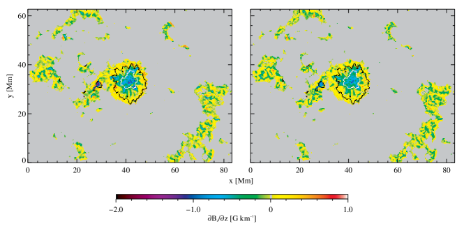
As an example, the results of Balthasar and Gömöry (2008) are displayed in Figure \ireffig:dbzdz. Bommier (2013) found values of the order of to G km-1. Balthasar et al. (2014b) obtained the main umbra of a -spot a shallow gradient of G km-1for ( is negative, therefore in Figure 9 of Balthasar et al., 2014b the gradient appears positive) and a much steeper gradient of G km-1in the -umbra of positive polarity. There is a weak trend that more recent data with higher spatial resolution yield steeper gradients of the vertical magnetic field with height.
| Author | spectral lines | umbra | penumbra |
|---|---|---|---|
| Hagyard et al. (1983) | C iv 154.6 nm | G km-1 | |
| Fe i 525.0 nm | |||
| Hofmann and | Fe i 525.0 nm | G km-1 | |
| Rendtel (1989) | Fe i 525.3 nm | ||
| Liu et al. (1996) | Fe i 532.42 nm | – G km-1 | |
| Balthasar (2006) | Fe i 1564.8 nm | – G km-1 | |
| Fe i 1089.6 nm | |||
| Balthasar and | Fe i 1078.3 nm | – G km-1 | 0 – G km-1 |
| Gömöry (2008) | Si i 1078.6 nm | ||
| Balthasar et al. (2013) | Fe i 1078.3 nm | – G km-1 | 0 – G km-1 |
| Si i 1078.6 nm | |||
| Bommier (2013) | Fe i 630.15 nm | – G km-1 | |
| Fe i 630.25 nm | |||
| Balthasar et al. (2014b) | Fe i 1078.3 nm | G km-1 | |
| Si i 1078.6 nm | G km-1(-U) |
At the outer edge of the penumbra and just outside, gradients of opposite sign are often found, indicating an increase of the vertical magnetic field component with height. Inside the penumbra, this can be explained by the inclination of the magnetic field. In deep layers, the magnetic field is almost horizontal with a very small vertical component. In higher layers, the magnetic field is less inclined, and the vertical component becomes significant. Just outside the penumbra, we encounter granulation, so that the total magnetic field is small in the deep layers. Further up, there is a magnetic canopy with a higher field strength.
4 Pores
S:pores
So far, we considered mature sunspots with a penumbra, but the same methods can be applied also to solar pores without a penumbra. Pores have a smaller magnetic field strength than sunspot umbrae, values of about 2000 G are found. The magnetic gradient is even steeper than for the umbra of larger sunspots. Muglach, Solanki, and Livingston (1994) determined G km-1 from a broadening excess of the -components of the Stokes- profile of the line Fe i 1564.8 nm in comparison to Fe i 1565.2 nm. Sütterlin (1998) measured gradients of G km-1 based on the bisectors of the Stokes- lobes. In a pore next to the sunspot, Balthasar and Gömöry (2008) found a value of even G km-1 for the total magnetic field strength and G km-1 for the vertical component from the difference method. This pore is visible in Figure \ireffig:BandG_bbh left of the main spot. From the divergence-free condition, the same authors obtained to G km-1 (see Figure \ireffig:dbzdz). There is a trend that pores exhibit steeper gradients than large spots. Such a trend is in agreement with model calculations presented by Osherovich (1984).
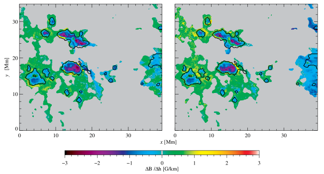
A group of pores connected via an arch filament system with a spot of opposite polarity was investigated by Balthasar et al. (2016) and Balthasar et al. (2018). The observations were performed with the GREGOR Infrared spectrograph (GRIS, Collados et al., 2012 at the GREGOR telescope. Only the magnetic field strength was determined from the spectral lines Ca i 1083.9 nm and the Si i 1082.7 nm, but magnetic gradients were not investigated. Therefore I revisited the data and present the height dependence of the magnetic field in the pores in Figure \ireffig:pores_dbdh. The steepest gradient of the total magnetic field strength in the main central pore amounts to G km-1. The average over the larger pores is G km-1. For the vertical component of the magnetic field an average gradient of G km-1 is obtained. The vertical component decreases steeper with height than the total field strength indicating that the magnetic field becomes more horizontal at a certain layer above the pores. The steepest gradient of the vertical component amounts to G km-1 and appears in one of the merging pores located above the central pore in Figure \ireffig:pores_dbdh. (For the temporal evolution of the pores see Balthasar et al., 2016).
Due to the short exposure times, these data are noisy, and the determination of magnetic gradients according to the divergence-free condition suffers from this limitation. While the mean values inside the pores are G km-1 for the calcium line and G km-1 for the silicon line, there are lanes dividing the pores into two halves where gradients of G km-1 and steeper are encountered.
5 Radio observations
S:radio
To measure magnetic fields in the corona, radio observations provide several possibilities, for an overview see White (2005). Magnetic field strengths of sunspots can be determined when gyro resonance emission appears above umbrae of sufficiently large size. Electrons spiral along magnetic field lines and emit radio radiation at harmonics of the electron gyro frequency, which is /357 GHz. Thus, the magnetic field strength can be determined according to the equation , where is the order of the harmonic. However, radio telescopes with spatial resolution operate only at selected frequencies. Akhmedov et al. (1982) used the RATAN-600 radio telescope (Berlin et al., 1977) at five different frequencies and measured also the degree of circular polarization. For different sunspots, they found field strengths between 1420 G and 2200 G. Together with the photospheric magnetic field strengths as they were published in Solnechnye Dannye, they arrived at a magnetic gradient shallower than G km-1. In general, the photospheric field strengths were between 200 and 600 G higher than those determined from the radio emission. A problem with such measurements on the solar disk is that the height of the origin of the radio emission can only be estimated under special assumptions and modeling.
Brosius and White (2006) observed layers above a sunspot at the solar limb with the Very Large Array (VLA) at frequencies of 8 and 15 GHz. From these spatially resolved observations above the solar limb, they precisely determined the height above the photosphere. They argued that the emission at 15 GHz corresponds to the third harmonic with a magnetic field strength of 1750 G at 8000 km above the photosphere. Similarly, they conclude that the field strength is 960 G at 12000 km. Assuming a photospheric field strength of 2600 G, these values lead to gradients of G km-1 and G km-1, respectively.
The atmosphere above sunspots is also investigated by Stupishin et al. (2018) based on RATAN-600 observations. In their Figure 3 they show gyro-resonance contours superposed on magnetograms for two different heights, but they do not explicitly discuss magnetic gradients. Taking the extreme values from both layers, one obtains a magnetic gradient of G km-1.
6 Magnetic flux considerations
S:flux
To probe whether the penumbra is deep or shallow, Solanki and Schmidt (1993) estimated the magnetic flux going through a dome-like hemisphere above the sunspot with a constant field strength as measured at the outer edge of the penumbra. Then they measured the flux of the umbra and found this value to be much smaller than the flux going through the hemisphere and concluded for a deep penumbra. Balthasar and Collados (2005) turned this idea around and measured the full Stokes-vector for a map covering a whole sunspot. From this map they determined the magnetic flux rising through the photosphere and found that it is less than the amount that would leave through a hemisphere. The measured amount of flux can leave through an ellipsoidal cap with a top height of 5250 km, while the radius of the spot is 9500 km. A Wilson depression of 800 km was assumed for these investigations. A sketch is shown in Figure \ireffig:ellipsoid. Balthasar and Gömöry (2008) confirmed this result, which is in agreement with the observations including a wider height range, but not with measurements from different photospheric lines. If this picture of a flat ellipsoid with a constant magnetic field strength represents an approximation to the real situation in a sunspot, it means that the magnetic field is less inclined in the chromosphere than in the photosphere. Magnetic field lines cross such a surface perpendicularly, and within the ellipsoid, the field has to expand horizontally. The magnetic field configuration would be goblet-like as the sketch in Figure \ireffig:goblet demonstrates. However, the magnetic field may be strongly structured in the upper chromosphere, and then such a picture will be invalid.

7 Horizontal pressure balance
S:p_balance
Once mature sunspots are formed, they appear rather stable for several days. Therefore, it is expected that they are in horizontal pressure equilibrium with their surroundings. The horizontal pressure balance is represented by Equation \irefEq_phor,
| (4) |
where is the external and the internal gas pressure. The magnetic pressure consists of two terms, where term represents the pressure due to the curvature of the field lines, which is often neglected because it is not easy to determine, and it is expected that this term is smaller than the main magnetic pressure term. However, this expectation is only justified when the curvature of the magnetic field lines is small enough, and with a larger curvature, the second term might be of the same order as the pressure term. The pressure is measured in Pa, therefore the factor 80.
Solanki, Walther, and Livingston (1993) investigated two different scenarios and put an upper limit of the decrease of the magnetic field to 2 G km-1 and 0.8 G km-1, respectively. The scenarios differ in the jump of the Wilson depression at the umbral boundary. Mathew et al. (2004) determined a map of the Wilson depression based on this method, but they gave no statement of the magnetic field gradient. Puschmann, Ruiz Cobo, and Martínez Pillet (2010) investigated a small area in the inner penumbra and obtained a gradient of G km-1. Sütterlin (1998) compared a model derived from pore observations with a photospheric model of Vernazza, Avrett, and Loeser (1976) and determined the magnetic field strength decrease to less than 5 – 6 G km-1. An investigation for penumbral flux tubes was presented by Borrero (2007), showing that the force equilibrium is guaranteed if the magnetic field possesses a transverse component.
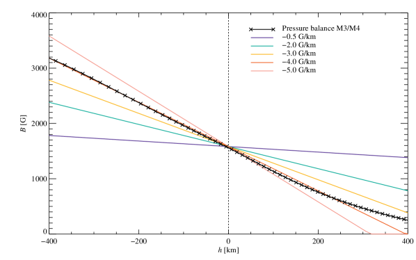
To study the pressure balance in more detail, I take a model for the outer atmosphere calculated with the CO5BOLD-code (Freytag, Steffen , and Dorch, 2002). Properties of this model are displayed in Kupka (2009). I consider the central umbra where curvature forces can be neglected because here magnetic field lines are straight. Models M3 and M4 of Stellmacher and Wiehr (1975) and Kollatschny et al. (1980) are combined, and the internal gas pressure from this models was taken. I assume that the magnetic field strength is 3000 G at the zero-height of the M4-model. With this assumption, the two height scales can be adjusted. For each height the magnetic field strength to balance the outer gas pressure is calculated, and the curve with the symbols in Figure \ireffig:balance is obtained. Linear curves for different magnetic gradients are also calculated to enable the comparison. Best agreement is obtained with a gradient of G km-1 in the lower photosphere. The curve flattens towards higher layers, but the gradient for the upper photosphere is still steeper than that for the divergence-free condition. A very similar picture is obtained when the umbral model of Maltby et al. (1986) is used instead of the M3/M4 models.
8 Numerical simulations
S:numsim
Nowadays, sophisticated numerical simulations of sunspots are available. A series of such simulations are presented by Rempel (2011a), Rempel (2011b), Rempel (2011c) and Rempel (2012). Although the information is contained in the models, he did not investigate in detail the height dependence of the magnetic field. A first attempt to determine the magnetic gradient was done by Jaeggli et al. (2012) who used the model of Rempel (2011c). They found a gradient of G km-1 from the model.
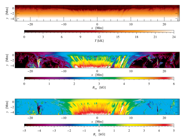
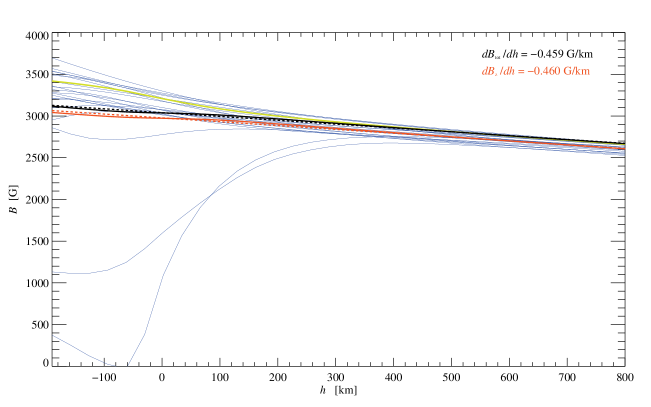
For a more detailed investigation, I used the model published in Rempel (2012). Vertical cross sections of the sunspot for temperature, total magnetic field strength and its vertical component are displayed in Figure \ireffig:rempel. Obviously the magnetic stratification depends on the location. At some positions, deep layers are even free of magnetic field. The geometrical height is set to zero where lg is zero in the umbra corresponding to a temperature of 4000 K. Therefore, Figure \ireffig:gradrempel shows the height dependence for several locations together with mean curves for the total magnetic field strength and for the vertical component for a more homogeneous central part of the umbra ( to +2.59 Mm in Figure \ireffig:rempel). Local differences occur mainly in the deep layers. The mean curves for and differ in the absolute values, but not in the gradients. Linear fits to the curves yield gradients of G km-1 and G km-1, respectively. These values are lower than those of Jaeggli et al. (2012) and correspond more to those obtained with the divergence-free method. Rempel (2012) configured the simulation such that the magnetic field strength in the spot drops from 6400 G at the bottom of his calculations to 2560 G at the top, and the calculation covers a height range of 6144 km, corresponding to a gradient of G km-1.
The averaged curves show an almost linear magnetic field gradient in all heights, and all curves for single locations show a linear behavior above a height of 300 km. For a majority of the curves from single locations, we see slightly steeper gradients in deep layers, but for a few locations, the magnetic field decreases towards deep layers, reaching even zero in one case. These locations have a strong impact when taking averages. The mean curve for the central part [, +0.54] Mm; green curve in Figure \ireffig:gradrempel, where no low field intrusions from below occur, shows a gradient of about G km-1 for heights below 200 km. This value corresponds to the value found by Jaeggli et al. (2012) and is in less agreement with the results obtained with divergence-free method, but it is also lower than the gradient from different photospheric lines.
9 Discussion
S:discussion
The discrepancy between the magnetic gradients obtained from different methods was topic of the workshop “The problem of the magnetic field gradients in sunspots” held in Meudon October 3 – 5, 2016 (in the following called the Meudon workshop). In this section, I pick up many aspects of the discussion at the workshop.
Maxwell’s theory of electromagnetism is well established, thus there are no doubts that the magnetic field is divergence-free. Local problems can arise when the spatial resolution is insufficient, and neighboring pixels belong to different fine structures which might reflect even different height layers. Figures \ireffig:BandG_bbh and \ireffig:tiwari8 demonstrate the internal structure of sunspots. Such a structure would create a bias of the horizontal partial derivatives, but it is hard to imagine how this effect could cause a systematically reduced decrease of the vertical magnetic field strength. It should also cause an increase at another location, and on average over the whole spot, it should show large fluctuations, but no systematic bias of the magnetic gradient. A more sophisticated investigation of this problem, suggested by Jean Heyvaerts, was discussed at the Meudon workshop leading to the result that this effect does not cause a significant violation of div = 0. For more details see Bommier (2014). At the Meudon workshop, Silvano Bonazzola suggested to investigate the effect of applying quotients of finite differences as approximations instead of the real derivatives to determine div . If the spatial variation scale of magnetic field is large with respect to the pixel size, finite difference and derivative are not very different, whereas if the magnetic field spatial variation scale is small or comparable to the pixel size, a difference may exist. But in this case, if the field lines are distorted inside a pixel face, the magnetic flux goes in and out as well, and the flux remains balanced. In this case, it remains unclear how the field line distortion can be responsible for an apparent flux loss, such as the one observed with a factor of about 10 between vertical and horizontal flux. In other words, the difference between finite difference and derivative results are too small to explain the observed difference between the gradients.
On the other hand, for a small sunspot the magnetic field strength reduces from an umbral value of about 2500 G to about 500 G at the outer edge of the penumbra. The radius of such a spot is about 10 000 km, and the horizontal gradient is in the order of 0.2 G km-1, too. And a steep gradient of G km-1 can be valid only over a limited height range. A magnetic field strength of 3000 G in deep layers would be reduced to zero at a layer 1500 km higher.
9.1 Formation height of spectral lines
Another uncertainty is the formation height of the spectral lines. Spectral lines are formed in an extended height range, and the mean value or the center of gravity of the contribution function or the response function are given as formation height. Nevertheless, height differences of 100 km or even more are used to obtain magnetic height gradients of G km-1 from the height difference method. To reduce these gradients, one has to increase the height differences by a factor of 5 – 10. The theory of stellar atmospheres tells us that the solar photosphere has an extension of less than 500 km, and with modern solar telescopes we resolve such a range, and we can prove that the extension is not larger than 500 km. Faurobert et al. (2009) directly measured the height difference of the two iron lines at 630.15 nm and 630.25 nm and found a value of 64 km, almost independent of the location on the Sun. This is the same difference as it was used by Balthasar et al. (2013) for their Hinode data. The uncertainty of the formation height is not the way out of the problem of the magnetic gradients.
In general, the linear polarization is weaker than the circular one. Therefore, the response of linear polarization to the magnetic field happens in deeper layers than that of circular polarization. This may impact the results for the magnetic vector, but a sophisticated inversion code is able to take this effect into account, if the observations contain enough height dependent information, and the physical parameters are calculated height dependent. Nevertheless, such inversions still yield steep magnetic gradients from height differences.
One may also argue that the results are affected from the properties of different detectors and different telescopes. However, Sánchez Cuberes, Puschmann, and Wiehr (2005) and Balthasar and Gömöry (2008) obtained their data from two spectral lines strictly simultaneously on the same detector, and both teams got steep gradients, although Sánchez Cuberes, Puschmann, and Wiehr (2005) performed a height dependent inversion, while Balthasar and Gömöry (2008) inverted their data independently for the two lines.
9.2 Does return flux play a rôle?
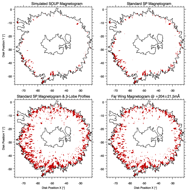
There are several hints that a part of the magnetic field lines in the outer penumbra are curved downward (Westendorp Plaza et al., 2001; del Toro Iniesta, Bellot Rubio, and Collados, 2001; Bellot Rubio, Balthasar, and Collados, 2004; Ruiz Cobo and Asensio Ramos, 2013; Franz et al., 2016). Osherovich and Garcia (1989) developed a sunspot model with return flux in the outer penumbra and found a good agreement with observations of unipolar and approximately round sunspots. In a detailed observational study, Franz and Schlichenmaier (2013) compared the occurrence of opposite polarities from the standard Hinode-SP magnetogram, from a simulation of a magnetogram mimicking observations with the Lockheed Solar Optical Universal Polarimeter (SOUP; Berger and Title, 2001) at the Swedish Solar Tower (SST; Scharmer et al., 2003), from a Hinode-SP magnetogram calculated for the far wings of the spectral line, and from a magnetogram considering 3-lobe profiles. While for standard magnetograms such as the first two only 4% of the penumbral pixel exhibit opposite polarities, the number increases to about 17% for the latter, more sensitive methods. Franz and Schlichenmaier (2013) conclude that opposite magnetic polarities are more frequent than one previously thought based on low spectral resolution measurements. The distribution of opposite polarities for the different types of magnetograms is displayed in Figure \ireffig:franz6.
Let us assume the spot consists of a bundle of flux tubes rising through the umbra. According to this amount of magnetic flux and the pressure conditions, the magnetic field configuration is adjusted with steep vertical and horizontal gradients. However, the horizontal field in the penumbra is extended, and therefore additional rising flux is required. Such flux may occur as almost horizontal flux tubes independent from the main spot. If flux rises and descends close together inside the penumbra, the additional flux will not be recognized at limited spatial resolution. Unresolved, it will look like an extended horizontal magnetic field. If resolved, one will see a salt-and-pepper pattern of ascending and descending magnetic field lines, and a decrease and increase of the horizontal components of the magnetic field. Then the horizontal gradient of the magnetic field appears shallower than in vertical direction above the umbra. The horizontal decrease according to the umbral flux will correspond to the vertical decrease, but new magnetic flux replenishes the horizontal field in lower layers of the outer penumbra. For the penumbra, this effect may be an explanation for the gradient differences among the different methods, but is hard to imagine that such an effect also acts in the umbra, where the magnetic field is less inclined.
9.3 Twist and writhe
Simple models for sunspots with twisted magnetic field have been presented by Osherovich and Flaa (1983) who considered a twist of the whole sunspot. The twist in these models is smaller in higher atmospheric layers and influences the structure of the sunspot only slightly. Seehafer (1990) studied the current helicity in sunspots and found the same sign of helicity in one hemisphere and the opposite sign in the other. This scenario was confirmed by Pevtsov, Canfield, and Metcalf (1995) and Zhang, Bao, and Kuzanyan (2002). However, it is a tendency but not a strict rule. As shown in Figure \ireffig:BandG_bbh, the magnetic field exhibits a local structure, which may arise from twist and writhe of bundles of flux tubes. As a consequence, the magnetic azimuth will rotate over a certain height range, and part of the polarization of the light will be canceled out. In this case, one may obtain a reduced magnetic field strength from spectral lines formed over a wider height range, which probe also the higher layers of the photosphere. A spectral line formed in deep layers probes only a narrow atmospheric layer and exhibits a strong magnetic field. There have been indications that magnetic twist plays a rôle in sunspots, especially in the penumbra. Borrero, Lites, and Solanki (2008) found opposite signs for the deviation of the azimuth from the radial direction on both sides of penumbral filaments, and explained this result by a magnetic field wrapping around the filament. An analysis of the torsion within a sunspot was performed by Socas-Navarro (2005) who concluded that flux ropes of opposite helicity may coexist in the same spot.
| Model | Si i 1082.7 nm | Ca i 1083.9 nm | Fe i 630.25 nm | Fe i 630.15 nm |
|---|---|---|---|---|
| M4_30_00_0 | 2650 G | 2740 G | 2710 G | 2720 G |
| M4_05_00_0 | 2930 G | 2940 G | 2950 G | 2950 G |
| M4_05_10_1 | 2900 G | 2930 G | 2930 G | 2910 G |
| M4_05_20_1 | 2830 G | 2920 G | 2850 G | 2760 G |
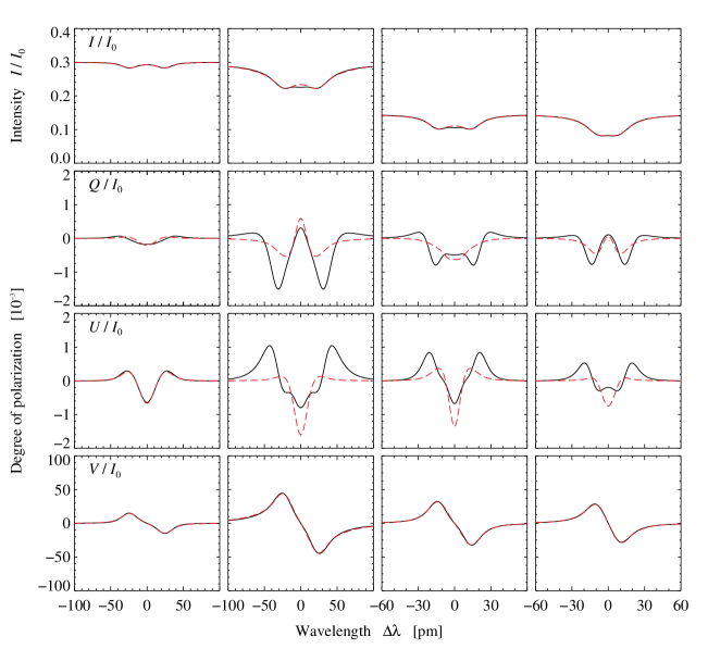
To investigate this idea, a test is performed. The umbral model atmosphere M4 of Kollatschny et al. (1980) with a height dependent magnetic field strength, but with zero values for the magnetic azimuth and inclination serves as starting model. The height range of the model is extrapolated up to lg. In the starting model M4_30_00_0, the magnetic field decreases from 3000 G at lg = 0 to 1500 G at lg, corresponding to a magnetic gradient of about G km-1. In the next step, this model is modified that the magnetic field strength decreases only to 2750 G at lg, corresponding to a magnetic gradient of about G km-1 (M4_05_00_0). Then an azimuth rotating with height and a height independent inclination are introduced. I assume one rotation over five units of lg . The inclination is 10∘ (M4_05_10_1) and 20∘ (M4_05_20_1). Thus the inclination points into different directions according to the magnetic azimuth, and therefore a magnetic field is modeled that winds around the line-of-sight. The corresponding Stokes-profiles are calculated for the spectral lines Si i 1082.7 nm, Ca i 1083.9 nm, Fe i 630.15 nm and Fe i 630.25 nm. These lines in general probe rather different layers of the photosphere, the Ca line forms in deep layers, while the Si line probes the upper photosphere (see Balthasar et al., 2016, Felipe et al., 2016). However, in the cold umbra, the height difference between the calcium line and the silicon line reduces to about 50 km. To calculate the line profiles, I used a macroturbulence of 2.0 km s-1, leading to a broadening of the profiles. Subsequently, SIR-inversions are performed with the line profiles from the different models independently for the individual lines. In these inversions, the magnetic parameters are treated as height-independent. This way, one obtains an average of the magnetic azimuth integrated over a certain height range weighted with the response or contribution function. The obtained linear polarization depends on this. The Ca line exhibits only a small change of the magnetic field strength with increasing number of azimuth windings, but the field strength from the silicon line decreases rapidly as Table \ireftbl:twist shows. The obtained gradients of the magnetic field are a bit shallower than the ones preset in the starting model, probably an effect of the introduced broadening. For M4_30_00_0 the gradient is G km-1and for M4_05_00_0 it is G km-1. Including twist, the gradients become steeper, G km-1 for an inclination of 10∘ and – G km-1 for an inclination of 20∘. A problem arises because Stokes- and then have many lobes of varying sign, what is not observed in sunspots. A comparison of the created profiles and the fits is given in Figure \ireffig:twistprofiles. Note that with the settings for the inversions, the linear polarization cannot be reproduced exactly. Perhaps this point is less important because the linear polarization created in the models is rather low.
In conclusion, twist and writhe may play a rôle, but the solar reality is not as simple as these tests. Another problem of such a scenario may be that many windings lead to magnetic instabilities such as the kink instability (see Török, Kliem, and Titov, 2004). It also remains unclear if this simple configuration fulfills the condition div = 0. More detailed and sophisticated investigations are required to arrive at a conclusive result about how twist and writhe can contribute to solve the discrepancy of the magnetic gradients from different methods.
9.4 Other ideas to explain the discrepancy of magnetic gradients from different methods
Bommier (2013) discussed that the Debye-volume is not a sphere because of the stratification of the solar atmosphere, and as a consequence typical horizontal and vertical length scales are different. This requires a re-scaling of typical lengths and affects the partial derivatives of the magnetic field, especially the vertical one. Bommier considered the vertical pressure scale height in comparison to the diameter of a typical photospheric structure such as a granule. However, the granular velocity structure can be followed over several hundred kilometers (almost the whole photospheric extension), and thus the aspect ratio is much smaller than she needs to explain the magnetic gradients. More relevant are the velocities. Over this height range, the vertical velocity changes from about 2 km s-1 to a horizontal expansion of about 1 km s-1 (Balthasar, 1985). This velocity pattern characterizes a granule. Again the ratio is too small. The situation is similar for sunspots which can be traced down to 40 Mm as shown by Chen et al. (1998) using helioseismic investigations. The discussion is ongoing, and perhaps the velocity difference between ions and electrons plays a more important rôle.
If a sunspot is composed of many flux tubes, the filling factor for the magnetic field may vary in different heights. This idea was suggested by Gerard Belmont and discussed during the Meudon workshop. A consideration by Pascal Démoulin at this workshop showed that a filling factor smaller than one will make the situation even worse, i.e. such a scenario will create steeper gradients.
Refraction in the solar atmosphere was suggested as a possible source of errors, but several investigations showed that refraction is negligible in the solar photosphere and chromosphere. Vincent, Scott, and Trampedach (2013) provide an equation for the refractive index including relativistic effects (their Equation 13). If we take the hydrogen density from model C of Vernazza, Avrett, and Loeser (1976) at lg = 0, the refractive index amounts to 1 + 5. Thus the deviation from unity is very small, and effects due to refraction can be neglected in the solar atmosphere. Even if they are not negligible, they will occur when observing perpendicular to the stratification of the atmosphere near the limb, while most sunspots were observed close to disk center, i.e. more along the density gradient. Therefore, atmospheric refraction is unlikely to contribute to the problem of the magnetic gradients.
10 Conclusions
The problem of the magnetic gradient in the photosphere of sunspots and pores remains unsolved. Observed gradients are much steeper when they are determined from different spectral lines or from single line making use of the atmospheric stratification than when the gradients are determined from the condition div = 0. In most cases, from the first method values between G km-1 and G km-1 were obtained, while applying the divergence-free condition yields values of G km-1 or even shallower. Additional investigations were presented, partly supporting steep gradients, e.g. the pressure balance to the stratification of the outer surroundings, and partly shallow gradients, e.g. the determination from a numerical simulation. All methods based on information from chromosphere lines exhibit shallow gradients of G km-1 or shallower. Radio observations cover an even larger height range and yield shallow gradients between G km-1 and G km-1. Since we know that the gas pressure of the quiet Sun decays exponentially with height, one should also expect a shallow gradient of the magnetic field for chromospheric layers and above. Thus the discrepancy between the different methods appears mainly in the photosphere.
Several options to explain the difference between the methods were discussed in the previous section, but most of them can be ruled out. The explanation cannot be found in the uncertainties of the height scale determinations nor in the influence of spatial resolution in the determination of the partial derivatives of the magnetic field. It appears that the final word is not spoken for the effects of twist and writhe. It seems likely that here at least a part of the answer could be found, but more sophisticated investigations are required, supported by numerical simulations.
Observations with the upcoming new solar facilities are also required. These instruments provide a better spatial resolution and will allow us to study the fine structure in sunspots in more details. There is indication that sunspots have an internal structure, not only when umbral dots appear, but also in the normal dark umbra. For example, with such high resolution investigations, it should be possible to obtain a clearer picture about twisted magnetic fields than we have at the moment, and judge how much twist and writhe really contribute to the problem of the magnetic gradients. However, better observations with higher resolution and polarimetric accuracy and sophisticated numerical simulations may reveal other explanations.
Acknowledgments
I am deeply indebted to Dr. Véronique Bommier for many discussions and comments on the topic. I also thank her and Prof. Carsten Denker for carefully reading the manuscript. Dr. Matthias Steffen provided me with a model atmosphere and Dr. Matthias Rempel with a cut through one of his numerical simulations. My thanks go also to Dr. Morten Franz and Dr. Sanjiv Tiwari for the permission to use their figures (Figure \ireffig:franz6 and Figure \ireffig:tiwari8). The 1.5-meter GREGOR solar telescope was built by a German consortium under the leadership of the Kiepenheuer Institute for Solar Physics in Freiburg with the Leibniz Institute for Astrophysics Potsdam, the Institute for Astrophysics Göttingen, and the Max-Planck-Institute for Solar System Research in Göttingen as partners, and with contributions by the Instituto de Astrofísica de Canarias and the Astronomical Institute of the Academy of Sciences of the Czech Republic.
Disclosure of Potential Conflicts of Interest The author declares that he has no conflicts of interest.
References
- Abdussamatov (1971) Abdussamatov, H.I.: 1971, On the magnetic fields and motions in sunspots at different atmospheric levels. Sol. Phys. 16, 384. DOI. ADS.
- Akhmedov et al. (1982) Akhmedov, S.B., Gelfreikh, G.B., Bogod, V.M., Korzhavin, A.N.: 1982, The measurement of magnetic fields in the solar atmosphere above sunspots using gyroresonance emission. Sol. Phys. 79, 41. DOI. ADS.
- Balthasar (1985) Balthasar, H.: 1985, On the contribution of horizontal granular motions to observed limb-effect curves. Sol. Phys. 99, 31. DOI. ADS.
- Balthasar (2006) Balthasar, H.: 2006, Vertical current densities and magnetic gradients in sunspots. A&A 449, 1169. DOI. ADS.
- Balthasar and Bommier (2009) Balthasar, H., Bommier, V.: 2009, The height dependence of the magnetic vector field in sunspots. In: Berdyugina, S.V., Nagendra, K.N., Ramelli, R. (eds.) Solar polarization 5 in honor of Jan Olof Stenflo, Astron. Soc. Pacific Conf. Ser. 405, 229. ADS.
- Balthasar and Collados (2005) Balthasar, H., Collados, M.: 2005, Some properties of an isolated sunspot. A&A 429, 705. DOI. ADS.
- Balthasar and Gömöry (2008) Balthasar, H., Gömöry, P.: 2008, The three-dimensional structure of sunspots I. The height dependence of the magnetic field. A&A 488, 1085. DOI. ADS.
- Balthasar and Schmidt (1993) Balthasar, H., Schmidt, W.: 1993, Polarimetry and spectroscopy of a simple sunspot II. On the height and temperature dependence of the magnetic field. A&A 279, 243. ADS.
- Balthasar et al. (2013) Balthasar, H., Beck, C., Gömöry, P., Muglach, K., Puschmann, K.G., Shimizu, T., Verma, M.: 2013, Properties of a decaying sunspot. Centr. Eur. Astrophys. Bull. 37, 435. ADS.
- Balthasar et al. (2014a) Balthasar, H., Beck, C., Louis, R.E., Verma, M., Denker, C.: 2014a, Near infrared spectropolarimetry of a -spot. A&A 562, L6. DOI. ADS.
- Balthasar et al. (2014b) Balthasar, H., Beck, C., Louis, R.E., Verma, M., Denker, C.: 2014b, The magnetic configuaration of a -spot. In: Nagendra, K.N., Stenflo, J.O., Qu, Z.Q., Sampoorna, M. (eds.) Solar polarization 7, Astron. Soc. Pacific Conf. Ser. 489, 39. ADS.
- Balthasar et al. (2016) Balthasar, H., Gömöry, P., González Manrique, S.J., Kuckein, C., Kavka, J., Kučera, A., Schwartz, P., Vaškova, R., Berkefeld, T., Collados Vera, M., Denker, C., Feller, A., Hofmann, A., Lagg, A., Nicklas, H., Orozco Suárez, D., Pastor Yabar, A., Rezaei, R., Schlichenmaier, R., Schmidt, D., Schmidt, W., Sigwarth, M., Sobotka, M., Solanki, S.K., Soltau, D., Staude, J., Strassmeier, K.G., Volkmer, R., von der Lühe, O., Waldmann, T.: 2016, Spectropolarimetric observation of an arch filament system with the GREGOR solar Telescope. Astron. Nachr. 337, 1050. DOI. ADS.
- Balthasar et al. (2018) Balthasar, H., Gömöry, P., González Manrique, S.J., Kuckein, C., Kučera, A., Schwartz, P., Berkefeld, T., Collados Vera, M., Denker, C., Feller, A., Hofmann, A., Schmidt, D., Schmidt, W., Sobotka, M., Solanki, S.K., Soltau, D., Staude, J., Strassmeier, K.G., Volkmer, R., von der Lühe, O.: 2018, Spectropolarimetric observations of an arch filament system with the GREGOR. In: Belluzi, L. (ed.) Solar polarization 8, Astron. Soc. Pacific Conf. Ser. Forthcoming volume, ArXiv:1804.01789. ADS.
- Bellot Rubio, Balthasar, and Collados (2004) Bellot Rubio, L.R., Balthasar, H., Collados, M.: 2004, Two magnetic components in sunspot penumbrae. A&A 427, 319. DOI. ADS.
- Berger and Title (2001) Berger, T.E., Title, A.M.: 2001, On the relation of G-band bright points to the photospheric magnetic field. ApJ 553, 449. DOI. ADS.
- Berlicki, Mein, and Schmieder (2006) Berlicki, A., Mein, P., Schmieder, B.: 2006, THEMIS/MSDP magnetic field measurements. A&A 445, 1127. DOI. ADS.
- Berlin et al. (1977) Berlin, A.B., Esepkina, N.A., Zverev, Y.K., Kajdanovskij, N.L., Korol’Kov, D.V., Kopylov, A.I., Korkin, E.I., Parijskij, Y.N., Ryzhkov, N.F., Soboleva, N.S., Stotskij, A.A., Shivris, O.N.: 1977, The new radio telescope of the USSR Academy of Sciences, RATAN-600. Pribory i Tekhnika Eksperimenta 5, 8. ADS.
- Bommier (2013) Bommier, V.: 2013, Reconciling the vertical and horizontal gradients of the sunspot magnetic field. Phys. Res. International 2013, ID 195403. DOI. ADS.
- Bommier (2014) Bommier, V.: 2014, Electromagnetism in a strongly stratified plasma showing an unexpected effect of the Debye shielding. Comptes Rendus Physique 15, 430. DOI. ADS.
- Bommier et al. (2007) Bommier, V., Landi Degl’Innocenti, E., Landolfi, M., Molodij, G.: 2007, UNNOFIT inversion of spectro-polarimetric maps observed with THEMIS. A&A 464, 323. DOI. ADS.
- Borrero (2007) Borrero, J.M.: 2007, The structure of sunspot penumbrae IV. MHS equilibrium for penumbral flux tubes and the origin of dark core penumbral filaments and penumbral grains. A&A 471, 967. DOI. ADS.
- Borrero, Lites, and Solanki (2008) Borrero, J.M., Lites, B.W., Solanki, S.K.: 2008, Evidence of magnetic field wrapping around penumbral filaments. A&A 481, L13. DOI. ADS.
- Brosius and White (2006) Brosius, J.W., White, S.M.: 2006, Radio measurements of the height of strong coronal magnetic fields above sunspots at the solar limb. ApJ 641, L69. DOI. ADS.
- Bruls et al. (1995) Bruls, J.H.M.J., Solanki, S.K., Rutten, R.J., Carlsson, M.: 1995, Infrared lines as probes of solar magnetic features VIII. Mg i 12m diagnostics of sunspots. A&A 293, 225. ADS.
- Chen et al. (1998) Chen, H.R., Chou, D.Y., Chang, H.K., Sun, M.T., Yeh, S.J., LaBonte, B., the TON Team: 1998, Probing the subsurface structure of active regions with the phase information in acoustic imaging. ApJ 501, L139. DOI. ADS.
- Collados et al. (1994) Collados, M., Martínez Pillet, V., Ruiz Cobo, B., del Toro Iniesta, J.C., Vázquez, M.: 1994, Observed differences between large and small sunspots. A&A 291, 622. ADS.
- Collados et al. (2007) Collados, M., Lagg, A., Díaz García, J.J., Hernández Suárez, E., López López, R., Páez Maña, E., Solanki, S.K.: 2007, Tenerife Infrared Polarimeter II. In: Heinzel, P., Dorotovič, I., Rutten, R.J. (eds.) The physics of chromospheric plasmas, Astron. Soc. Pacific Conf. Ser. 368, 611. ADS.
- Collados et al. (2012) Collados, M., López, R., Páez, E., Hernández, E., Reyes, M., Calcines, A., Ballesteros, E., Diaz, J.J., Denker, C., Lagg, A., Schlichenmaier, R., Schmidt, W., Solanki, S.K., Strassmeier, K.G., von der Lühe, O., Volkmer, R.: 2012, GRIS: The GREGOR infrared spectrograph. Astron. Nachr. 333, 872. DOI. ADS.
- del Toro Iniesta, Bellot Rubio, and Collados (2001) del Toro Iniesta, J.C., Bellot Rubio, L.R., Collados, C.: 2001, Cold, supersonic Evershed downflows in a sunspot. ApJ 549, L139. DOI. ADS.
- Denker et al. (2016) Denker, C., Heibel, C., Rendtel, J., Arlt, K., Balthasar, J.H., Diercke, A., González Manrique, S.J., Hofmann, A., Kuckein, C., Önel, H., Senthamizh Pavai, V., Staude, J., Verma, M.: 2016, Solar physics at the Einstein Tower. Astron. Nachr. 337, 1105. DOI. ADS.
- Dunn (1969) Dunn, R.B.: 1969, Sacramento Peak’s new solar telescope. Sky & Tel. 38, 368. ADS.
- Eibe et al. (2002) Eibe, M.T., Aulanier, G., Faurobert, M., Mein, P., Malherbe, J.M.: 2002, Vertical structure of sunspots from THEMIS observations. A&A 381, 290. DOI. ADS.
- Faurobert et al. (2009) Faurobert, M., Aime, C., Périni, C., Uitenbroek, H., Grec, C., Arnaud, J., Ricort, G.: 2009, Direct measurement of the formation height difference of the 630 nm Fe i solar lines. A&A 507, L29. DOI. ADS.
- Felipe et al. (2016) Felipe, T., Collados, M., Khomenko, L., Kuckein, C., Asensio Ramos, A., Balthasar, H., Berkefeld, T., Denker, C., Feller, A., Franz, M., Hofmann, A., Joshi, J., Kiess, C., Lagg, A., Nicklas, H., Orozco Suárez, D., Pastor Yabar, A., Rezaei, R., Schlichenmaier, R., Schmidt, D., Schmidt, W., Sigwarth, M., Sobotka, M., Solanki, S.K., Soltau, D., Staude, J., Strassmeier, K.G., Volkmer, R., von der Lühe, O., Waldmann, T.: 2016, Three-dimensional structure of a sunspot light bridge. A&A 596, A59. DOI. ADS.
- Franz and Schlichenmaier (2013) Franz, M., Schlichenmaier, R.: 2013, The velocity field of sunspot penumbrae II. Return flow and magnetic fields of opposite polarity. A&A 550, A97. DOI. ADS.
- Franz et al. (2016) Franz, M., Collados, M., Bethge, C., Schlichenmaier, R., Borrero, J.M., Schmidt, W., Lagg, A., Solanki, S.K., Berkefeld, T., Kiess, C., Rezaei, R., Schmidt, D., Sigwarth, M., Soltau, D., Volkmer, R., von der Luhe, O., Waldmann, T., Orozco, D., Pastor Yabar, A., Denker, C., Balthasar, H., Staude, J., Hofmann, A., Strassmeier, K., Feller, A., Nicklas, H., Kneer, F., Sobotka, M.: 2016, Magnetic fields of opposite polarity in sunspot penumbrae. A&A 596, A4. DOI. ADS.
- Freytag, Steffen , and Dorch (2002) Freytag, B., Steffen , M., Dorch, B.: 2002, Spots on the surface of Betelgeuse – Results from the new 3D stellar convection models. Astron. Nachr. 323, 213. DOI. ADS.
- Frutiger et al. (2000) Frutiger, C., Solanki, S.K., Fligge, M., Bruls, J.H.M.J.: 2000, Properties of the solar granulation obtained from the inversion of low spatial resolution spectra. A&A 358, 1109. ADS.
- Gelly (2007) Gelly, B.F.: 2007, THEMIS Instrumentation and strategy for the Future. In: Heinzel, P., Dorotovič, K.N., Rutten, R.J. (eds.) The physics of chromospheric plasmas, Astron. Soc. Pacific Conf. Ser. 368, 593. ADS.
- Grigoryev et al. (1985) Grigoryev, V.M., Grigor’ev, V.M., Kobanov, N.I., Osak, B.F., Selivanov, V.L., Stepanov, V.E.: 1985, The vector magnetograph of the Sayan Solar Observatory. In: Hagyard, M.J. (ed.) Measurements of Solar Magnetic Vector Fields, NASA Conf. Publ. 2374, 231. ADS.
- Hagyard et al. (1983) Hagyard, M.J., Teuber, D., West, E.A., Tandberg-Hanssen, E., Henze, W., Beckers, J.M., Bruner, M., Hyder, C.L., Woodgate, B.E.: 1983, Vertical gradients of sunspot magnetic fields. Sol. Phys. 84, 13. DOI. ADS.
- Hale (1908) Hale, G.E.: 1908, On the probable existence of a magnetic field in sunspots. ApJ 28, 315. DOI. ADS.
- Henze et al. (1982) Henze, W., Tandberg-Hanssen, E., Hagyard, M.J., Woodgate, B.E., Shine, R.A., Beckers, J.M., Bruner, M., Gurman, J.B., Hyder, C.L., West, E.A.: 1982, Observations of the longitudinal magnetic field in the transition region and photosphere of a sunspot. Sol. Phys. 81, 231. DOI. ADS.
- Hewagama et al. (1993) Hewagama, T., Deming, D., Jennings, D., Osherovich, V., Wiedemann, G., Zipoy, D., Mickey, D.L., Garcia, H.: 1993, Solar magnetic field studies using the 12 micron emission lines. II. Stokes profiles and vector field samples in sunspots. ApJS 86, 313. DOI. ADS.
- Hofmann and Rendtel (1989) Hofmann, A., Rendtel, J.: 1989, Analysis and results of cooperative magnetographic measurements III. Vertical gradients of the magnetic field in the sunspot photosphere. Astron. Nachr. 310, 61. DOI. ADS.
- Ichimoto et al. (2008) Ichimoto, K., Lites, B., Elmore, D., Suematsu, Y., Tsuneta, S., Katsukawa, Y., Shimizu, T., Shine, R., Tarbell, T., Title, A., Kiyohara, J., Shinoda, K., Card, G., Lecinski, A., Streander, K., Nakagiri, M., Miyashita, M., Noguchi, M., Hoffmann, C., Cruz, T.: 2008, Polarization calibration of the Solar Optical Telescope onboard Hinode. Sol. Phys. 249, 233. DOI. ADS.
- Jaeggli et al. (2010) Jaeggli, S.A., Lin, H., Mickey, D.L., Kuhn, J.R., Hegwer, S.L., Rimmele, T.R., Penn, M.J.: 2010, FIRS: a new instrument for photospheric and chromospheric studies at the DST. Mem. S. A. It. 81, 763. ADS.
- Jaeggli et al. (2012) Jaeggli, S.A., Lin, H., Uitenbroek, H., Rempel, M.: 2012, Comparison of multi-height observations with a 3D MHD sunspot model. In: Golub, L., De Moortel, I., Shimizu, T. (eds.) Fifth Hinode Science Meeting: Exploring the active Sun, Astron. Soc. Pacific Conf. Ser. 456, 67. ADS.
- Jefferies, Lites, and Skumnaich (1989) Jefferies, J., Lites, B.W., Skumnaich, A.: 1989, Transfer of line radiation in a megnetic field. ApJ 343, 920. DOI. ADS.
- Joshi et al. (2016) Joshi, J., Lagg, A., Solanki, S.K., Feller, A., Collados, D. M. Orozco Suárez, Schlichenmaier, R., Franz, M., Balthasar, H., Denker, C., Berkefeld, T., Hofmann, A., Kiess, C., Nicklas, H., Pastor Yabar, A., Rezaei, R., Schmidt, D., Schmidt, W., Sobotka, M., Soltau, D., Staude, J., Strassmeier, K.G., Volkmer, R., von der Lühe, O., Waldmann, T.: 2016, Upper chromospheric magnetic field of a sunspot penumbra: observations of fine structure. A&A 596, A8. DOI. ADS.
- Joshi et al. (2017a) Joshi, J., Lagg, A., Hirzberger, J., Solanki, S.K.: 2017a, Three-dimensional magnetic structure of a sunspot: Comparison of the photosphere and upper chromosphere. A&A 604, A98. DOI. ADS.
- Joshi et al. (2017b) Joshi, J., Lagg, A., Hirzberger, J., Solanki, S.K., Tiwari, S.K.: 2017b, Vertical magnetic field gradient in the photosphereric layers of sunspots. A&A 599, A35. DOI. ADS.
- Kollatschny et al. (1980) Kollatschny, W., Stellmacher, G., Wiehr, E., Falipou, M.A.: 1980, The infrered Ca+ lines in sunspot umbrae. A&A 86, 245. ADS.
- Kosugi et al. (2007) Kosugi, T., Matsuzaki, K., Sakao, T., Shimizu, T., Sone, Y., Tachikawa, S., Hashimoto, T., Minesugi, K., Ohnishi, A., Yamada, T., Tsuneta, S., Hara, H., Ichimoto, K., Suematsu, Y., Shimojo, M., Watanabe, T., Shimada, S., Davis, J.M., Hill, L.D., Owens, J.K., Title, A.M., Culhane, J.L., Harra, L.K., Doschek, G.A., Golub, L.: 2007, The Hinode (Solar-B) Mission: An overview. Sol. Phys. 243, 3. DOI. ADS.
- Kupka (2009) Kupka, F.: 2009, Turbulent convection and numerical simulations in solar and stellar astrophysics. In: Hillebrandt, W., Kupka, F. (eds.) Interdisciplinary Aspects of Turbulence, Lecture Notes in Physics, Springer, Berlin, Germany, Lecture Notes in Physics, Springer, Berlin, Germany 756, 49. ADS.
- Lagg et al. (2004) Lagg, A., Woch, J., Krupp, N., Solanki, S.K.: 2004, Retrieval of the full magnetic vector with the He i multiplet at 1083 nm. Maps of an emerging flux region. A&A 414, 1109. DOI. ADS.
- Liu et al. (1996) Liu, Y., Wang, J., Yan, Y., Ai, G.: 1996, Gradients of the line-of-sight magnetic fields in active region NOAA 6659. Sol. Phys. 169, 79. DOI. ADS.
- Maltby et al. (1986) Maltby, P., Averett, E.H., Carlsson, M., Kjeldset-Moe, O., Kurucz, R.L., Loeser, R.: 1986, A new sunspot umbral model and its variation with the solar cycle. ApJ 306, 284. DOI. ADS.
- Mathew et al. (2003) Mathew, S.K., Lagg, A., Solanki, S.K., Collados, M., Borrero, J.M., Berdyugina, S., Krupp, N., Woch, J., Frutiger, C.: 2003, Three dimensional structure of a regular sunspot from the inversion of IR Stokes profiles. A&A 410, 695. DOI. ADS.
- Mathew et al. (2004) Mathew, S.K., Solanki, S.K., Lagg, A., Collados, M., Borrero, J.M., Berdyugina, S.: 2004, Thermal-magnetic in a sunspot and a map of its Wilson depression. A&A 422, 693. DOI. ADS.
- Moran et al. (2000) Moran, T., Deming, D., Jennings, D.E., McCabe, G.: 2000, Solar magnetic field studies using the 12 micron emission lines. III. Simultaneous measurements at 12 and 1.6 microns. ApJ 553, 1035. DOI. ADS.
- Muglach, Solanki, and Livingston (1994) Muglach, K., Solanki, S.K., Livingston, W.C.: 1994, Preliminary properties of pores derived from 1.56 micron lines. In: Rutten, R.J., Schrijver, C.J. (eds.) Solar Surface magnetism, NATO Advanced Science Institutes (ASI) Series C 433, 127. ADS.
- Orozco Suárez, Lagg, and Solanki (2005) Orozco Suárez, D., Lagg, A., Solanki, S.K.: 2005, Photospheric and chromospheric magnetic structure of a sunspot. In: Innes, D., Lagg, A., Solanki, S.K., Danesy, D. (eds.) Chromospheric and coronal magnetic fields, ESA, ESA SP-596, 59. ADS.
- Osherovich (1984) Osherovich, V.A.: 1984, A note on the values of the vertical gradient of the magnetic field in the return flux sunspot model. Sol. Phys. 90, 31. DOI. ADS.
- Osherovich and Flaa (1983) Osherovich, V.A., Flaa, T.: 1983, Sunspot models with twisted magnetic field. Sol. Phys. 88, 109. DOI. ADS.
- Osherovich and Garcia (1989) Osherovich, V.A., Garcia, H.A.: 1989, The relationship of sunspot magnetic fields to umbral sizes in return flux theory. ApJ 336, 468. DOI. ADS.
- Pahlke and Wiehr (1990) Pahlke, K.D., Wiehr, E.: 1990, Magnetic field, relative Dopppler shift and temperature for an inhomogeneous model of sunspot umbrae. A&A 228, 246. ADS.
- Pevtsov, Canfield, and Metcalf (1995) Pevtsov, A.A., Canfield, R.C., Metcalf, T.R.: 1995, Latitudinal variation of helicity of photospheric magnetic fields. ApJ 440, L109. DOI. ADS.
- Pierce (1964) Pierce, A.K.: 1964, The McMath solar telescope of Kitt Peak National Observatory. Appl. Opt. 3, 1337. DOI. ADS.
- Puschmann, Ruiz Cobo, and Martínez Pillet (2010) Puschmann, K.G., Ruiz Cobo, B., Martínez Pillet, V.: 2010, A geometrical height scale for sunspot penumbrae. ApJ 720, 1417. DOI. ADS.
- Rempel (2011a) Rempel, M.: 2011a, Penumbral fine structure and driving mechanisms of large-scale flows in simulated sunspots. ApJ 729, 5. DOI. ADS.
- Rempel (2011b) Rempel, M.: 2011b, Subsurface magnetic field and flow structure of simulated sunspots. ApJ 740, 15. DOI. ADS.
- Rempel (2011c) Rempel, M.: 2011c, Three-D numerical MHD modeling of sunspots with radiation transport. In: Choudhary, D.P., Strassmeier, K.G. (eds.) The Physics of Sun and Starspots, IAU Symp. 273, 8. DOI. ADS.
- Rempel (2012) Rempel, M.: 2012, Numerical sunspot models: Robustness of photospheric velocity and magnetic field structure. ApJ 750, 62. DOI. ADS.
- Rüedi, Solanki, and Livingston (1995) Rüedi, I., Solanki, S.K., Livingston, W.C.: 1995, Infrared lines as probes of solar magnetic features X. He i 10830 Å as a diagnostic of chromospheric magnetic fields. A&A 293, 252. ADS.
- Ruiz Cobo and Asensio Ramos (2013) Ruiz Cobo, B., Asensio Ramos, A.: 2013, Returning magnetic flux in sunspot penumbrae. A&A 549, L4. DOI. ADS.
- Ruiz Cobo and del Toro Iniesta (1992) Ruiz Cobo, B., del Toro Iniesta, J.C.: 1992, Inversion of Stokes profiles. ApJ 398, 375. DOI. ADS.
- Sánchez Cuberes, Puschmann, and Wiehr (2005) Sánchez Cuberes, M., Puschmann, K.G., Wiehr, E.: 2005, Spectropolarimetry of a sunspot at disk centre. A&A 440, 345. DOI. ADS.
- Schad et al. (2015) Schad, T.A., Penn, M.J., Lin, H., Tritschler, A.: 2015, Vector magnetic field maps of a sunspot and its superpenumbral fine-structure. Sol. Phys. 290, 1607. DOI. ADS.
- Scharmer et al. (2003) Scharmer, G.B., Bjelskjo, K., Korhonen, T.K., Lindberg, B., Petterson, B.: 2003, The 1-meter Swedish Solar Telescope. In: Keil, S.L., Avakyan, S.V. (eds.) Proc. SPIE 4853, 341. DOI. ADS.
- Schmidt et al. (2012) Schmidt, W., von der Lühe, O., Volkmer, R., Denker, C., Solanki, S.K., Balthasar, H., Bello González, N., Berkefeld, T., Collados, M., Fischer, A., Halbgewachs, C., Heidecke, F., Hofmann, A., Kneer, F., Lagg, A., Nicklas, H., Popow, E., Puschmann, K.G., Schmidt, D., Sigwarth, M., Sobotka, M., Soltau, D., Staude, J., Strassmeier, K.G., Waldmann, T.: 2012, The 1.5 meter solar telescope GREGOR. Astron. Nachr. 333, 796. DOI. ADS.
- Seehafer (1990) Seehafer, N.: 1990, Electric ccurrent helicity in the solar atmosphere. Sol. Phys. 125, 219. DOI. ADS.
- Socas-Navarro (2005) Socas-Navarro, H.: 2005, The three-dimensional structure of a sunspot magnetic field. ApJ 631, L167. DOI. ADS.
- Solanki and Schmidt (1993) Solanki, S.K., Schmidt, H.U.: 1993, Are sunspot penumbrae deep or shallow? A&A 267, 287. ADS.
- Solanki, Walther, and Livingston (1993) Solanki, S.K., Walther, U., Livingston, W.: 1993, Infrared lines as probes of solar magnetic features VI. The thermal-magnetic relation and Wilson depression of a simple sunspot. A&A 277, 639. ADS.
- Solanki (2003) Solanki, S.K.: 2003, Sunspots: An overview. A&A Rev. 11, 153. DOI. ADS.
- Stellmacher and Wiehr (1975) Stellmacher, G., Wiehr, E.: 1975, The deep layers of sunspot umbrae. A&A 45, 69. ADS.
- Stupishin et al. (2018) Stupishin, A.G., Kaltman, T.I., Bogod, V.M., Yasnov, L.V.: 2018, Modeling of solar atmosphere parameters above sunspots using RATAN-600 microwave observations. Sol. Phys. 293, 13. DOI. ADS.
- Sütterlin (1998) Sütterlin, P.: 1998, Properties of solar pores. A&A 333, 305. ADS.
- Tiwari et al. (2015) Tiwari, S.K., van Noort, M., Solanki, S.K., Lagg, A.: 2015, Depth dependent global properties of a sunspot observed by Hinode using the Solar Optical Telescope/Spectropolarimeter. A&A 583, A119. DOI. ADS.
- Török, Kliem, and Titov (2004) Török, T., Kliem, B., Titov, V.S.: 2004, Ideal kink instability of a magnetic loop equilibrium. A&A 413, L27. DOI. ADS.
- Tsuneta et al. (2008) Tsuneta, S., Ichimoto, K., Katsukawa, Y., Nagata, S., Otsubo, M., Shimizu, T., Suematsu, Y., Nakagiri, M. M.and Noguchi, Tarbell, T., Title, A., Shine, R., Rosenberg, W., Hoffmann, C., Jurcevich, B., Kushner, G., Levay, M., Lites, B., Elmore, D., Matsushita, T., Kawaguchi, N., Saito, H., Mikami, I., Hill, L.D., Owens, J.K.: 2008, The Solar Optical Telescope for the Hinode mission: An Overview. Sol. Phys. 249, 167. DOI. ADS.
- Verma et al. (2018) Verma, M., Denker, C., Balthasar, C. H. Kuckein, Rezaei, R., Sobotka, M., Deng, N., Wang, H., Tritschler, A., Collados, M., Diercke, A., González Manrique, S.J.: 2018, High-resolution imaging and near-infrared spectroscopy of penumbral decay. A&A 614, A2. DOI. ADS.
- Vernazza, Avrett, and Loeser (1976) Vernazza, J.E., Avrett, E.H., Loeser, R.: 1976, Structure of the solar chromosphere. II - The underlying photosphere and temperature-minimum region. ApJS 30, 1. DOI. ADS.
- Vincent, Scott, and Trampedach (2013) Vincent, A., Scott, P., Trampedach, R.: 2013, Light bosons and photspheric solutions to the solar abundance problem. MNRAS 432, 3332. DOI. ADS.
- von der Lühe (1998) von der Lühe, O.: 1998, High-resolution observations with the German Vacuum Tower Telescope on Tenerife. New Astron. Rev. 42, 493. DOI. ADS.
- Westendorp Plaza et al. (2001) Westendorp Plaza, C., del Toro Iniesta, J.C., Ruiz Cobo, B., Martínez Pillet, V., Lites, B.W., Skumanich, A.: 2001, Optical tomography of a sunspot II. Vector magnetic field and temeprature stratification. ApJ 547, 1130. DOI. ADS.
- White (2005) White, S.M.: 2005, Radio measurements of coronal magnetic fileds. In: Innes, D., Lagg, A., Solanki, S.K., Danesy, D. (eds.) Chromospheric and coronal magnetic fields, ESA SP-596, 10. ADS.
- Wittmann (1974) Wittmann, A.: 1974, Computation and observation of Zeeman multiplet polarization in Fraunhofer lines III. Magnetic field structure of spot Mt. Wilson 18488. Sol. Phys. 36, 29. DOI. ADS.
- Woodgate et al. (1980) Woodgate, B.E., Tandberg-Hanssen, E.A., Bruner, E.C., Beckers, J.M., Brandt, J.C., Henze, W., Hyder, C.L., Kalet, M.W., Kenny, P.J., Knox, E.D., Michalitsianos, A.G., Rehse, R., Shine, R.A., Tinsley, H.D.: 1980, The Ultraviolet Spectrometer and Polarimeter on the Solar Maximum Mission. Sol. Phys. 65, 73. DOI. ADS.
- Zhang, Bao, and Kuzanyan (2002) Zhang, H., Bao, S., Kuzanyan, K.M.: 2002, Twist of magnetic fields in solar active regions. Astron. Rep. 46, 424. DOI. ADS.