Uncertainty-Complementarity Balance as a General Constraint on Non-locality

Abstract

We propose an uncertainty-complementarity balance relation and build quantitative connections among non-locality, complementarity, and uncertainty. Our balance relation, which is formulated in a theory-independent manner, states that for two measurements performed sequentially, the complementarity demonstrated in the first measurement in terms of disturbance is no greater than the uncertainty of the first measurement. Quantum theory respects our balance relation, from which the Tsirelson bound can be derived, up to an inessential assumption. In the simplest Bell scenario, we show that the bound of Clauser-Horne-Shimony-Holt inequality for a general non-local theory can be expressed as a function of the balance strength, a constance for the given theory. As an application, we derive the balance strength as well as the nonlocal bound of Popescu-Rohrlich box. Our results shed light on quantitative connections among three fundamental concepts, i.e., uncertainty, complementarity and non-locality.

Introduction— The core formulation of quantum mechanics (QM) is based on the structures of Hilbert space, which gives rise to fundamental non-classical features such as uncertainty, complementarity, and non-locality. However, it is still an open question with respect to the underlying physical principles behind the structures of Hilbert space. This is quite unlike other successful theories such as the theory of relativity and statistical mechanics, whose formalisms can be directly derived from several fundamental physical principles. One fruitful approach to tackle the problem is to trace various quantum features back to its physical principles hall ; sp ; t1 ; t2 ; gpt ; nb ; gs ; Barr ; tn1 ; tn2 ; tn3 in a theory-independent manner. For examples, Bell has provided a general framework to quantify non-locality bel , within which the observed bipartite correlations precludes local realistic models of QM. Barrett introduced a framework applicable to generalized probabilistic theories t1 ; t2 ; gpt ; nb ; gs ; Barr in which, some properties thought special to QM, $e.g.$, teleportation  ta ; te , purification pur , coherencewoc , and entanglement swapping sw , have been found to be not confined to QM.

Actually, most of our understandings of QM in an axiomatic manner are gained by singling out QM based on the non-locality demonstrated by the correlations of compatible measurements. Many efforts have been devoted to understanding why quantum correlation is strong enough to be nonlocal but not so strong to be maximum nonlocal ns . For example, the Clauser-Horne-Shimony-Holt (CHSH) inequality has an upper bound 2 for any local realistic theory, the Tsirelson bound $2\sqrt{2}$ for QM bel , and reaches its maximum 4 for the Popescu-Rohrlich box model (PR-box) pr . Various principles have been proposed, $e.g.$, the information causality principle ic , nontrivial communication complexity wvd , global exclusion principle cl ; by ; ca , to explain the quantum mechanical non-local bound. While these results have gained some valuable insights to this question, they do not explain in a quantitative manner the intrinsic complementarity and uncertainty that are present in any general nonlocal theory gpt ; nb ; gs ; Barr ; ns ; hor . So far, the complementarity is taken only intuitively as a necessary condition for a non-local theory to respect the no-instantaneous communication principle tn1 . Hence, a natural question arises as to whether one can quantitatively determine the nonlocality bound with uncertainty and complementarity for a general theory, and then explain the Tsirelson bound.

In this Letter we give an answer to the above question by introducing an uncertainty-complementarity balance relation which is shown to impose a strong constraint on non-locality. For this purpose we consider the scenario in which two measurements, which might not be compatible to each other in comparison with compatible measurements in the usual Bell scenario, are performed sequentially. Our balance relation states that the complementarity demonstrated in the second measurement in terms of disturbance is no greater than the uncertainty presented in the first measurement. The balance relation is shown to be respected by QM and can account for the Tsirelson bound, together with an additional assumption. Essential in our balance relation there is a constance called balance strength for each specific theory. It turns out that the balance constance is intimately related to the non-locality: the bound of $\operatorname{CHSH}$ inequality for a specific theory can be casted into a function of its balance strength, from which we reproduce the non-local bound of PR-box as an application. Vise versa, non-locality displayed by a theory also imposes a constraint on the possible values of its balance strength.

Uncertainty and Complementarity balance — To start with, we assume that a given physical system can be in different states, which are nothing else than some mathematical structures that help to determine the statistics of all possible measurements performed on the system. For a given state of the system, each measurement, e.g., $A$, will result in a probability distribution, e.g., $\{p(a|A)\}$, over all possible outcomes of the measurement. Uncertainty of the measurement $A$ can be quantified in various ways and here we shall take

$$\delta_{A}=\left(\textstyle\sum_{a}\sqrt{p({a|A})}\right)^{2}-1$$ (1)

as the measure of uncertainty. Specially, if observable $A$ is a two-outcome observable with assigned values $\{0,1\}$, we have $\delta_{A}^{2}=4p(0|A)p(1|A)=1-\bar{A}^{2}$ with $\bar{A}=p(0|A)-p(1|A)$ being the expectation of the observable $A$.

Complementarity states that there are pairs of incompatible properties that cannot be measured simultaneously. Consequently one measurement might cause inevitable disturbance to a later incompatible measurement. Thus we consider two incompatible measurements performed in sequel. Here we consider only sharp measurements, measurements that are accurate and repeatable sm1 ; sm2 , for the sake of clarity. After a sharp measurement $A$, depending on the outcome $\mu$, the system might be brought into some states $\mathcal{S}_{\mu|A}$ that might be different from the original stats with probability $p({\mu|A})$. This state is conveniently referred to as the “eigenstate” of observable $A$. On average the output state after the measurement $A$ would be an ensemble $\{p({\mu|A}),\mathcal{S}_{\mu|A}\}$ of eignestates. And then the second measurement $A^{\prime}$ is performed on this ensemble, resulting in a probability distribution

$$p_{a|A\to A^{\prime}}=\sum_{\mu}p({\mu|A})P({a|A^{\prime},\mathcal{S}_{\mu|A}}),$$ (2)

where $P({i|A^{\prime},\mathcal{S}_{\mu|A}})$ denotes the probability of obtaining $i$ when measuring $A^{\prime}$ on $\mathcal{S}_{\mu|A}$. Had the first measurement of $A$ not been performed the measurement of $A^{\prime}$ on the original state would give rise to the statistics $\{p({a^{\prime}|A^{\prime}})\}$ instead. Therefore the difference between these two probability distributions

$$D_{A\rightarrow A^{\prime}}=\sum_{a}\big{|}p({a|A^{\prime}})-p({a|A\to A^{\prime}})\big{|}$$ (3)

quantifies naturally the disturbance of the second measurement ($A^{\prime}$) caused by the first measurement ($A$) and thus provides a quantitative measure of complementarity. We note that the above measures of uncertainty and disturbance involve only probabilities thus they do not rely on specific structure of potential theory.

Quantum mechanically, the relations between uncertainty and complementarity have been extensively studied in terms of measurement-disturbance relations  qu1 ; qu2 , where the complementarity is commonly lower-bounded by a function of uncertainty sss . On the other hand, since a measurement with zero uncertainty can not lead to a non-zero disturbance to a subsequent measurement, the complementarity should also impose some kinds of constraints on possible uncertainty of the first measurement. Quantum mechanically, a projective measurement $A^{\prime}$ is preformed after another projective measurement $A$ it holds (See SM)

$$\delta_{A}\geq D_{A\rightarrow A^{\prime}},$$ (4)

meaning that a measurement $A$ would not lead a disturbance $D_{A\rightarrow A^{\prime}}$ (to a following measurement $A^{\prime}$) greater than its uncertainty $\delta_{A}$. We note that the quantum mechanical balance relation Eq.(4) can be saturated: $\delta_{A}=1$ and $D_{A\rightarrow A}=1$ for a qubit in the state $\rho=|0\rangle\langle 0|$ with two measurements $A=\sigma_{x}$ and $A^{\prime}=\sigma_{z}$, then .

Now we are in the position to introduce a general balance relation similar to Eq.(4) for any probabilistic theory. By denoting

$$\alpha=\sup\{\alpha^{\prime}\geq 0|\delta_{A}\geq\alpha^{\prime}D_{A\rightarrow A^{\prime}}\ (\forall A,A^{\prime},\mathcal{S})\}$$ (5)

our generalized balance relation reads

$$\delta_{A}\geq\alpha D_{A\rightarrow A^{\prime}}.$$ (6)

The balance strength can be taken as a benchmark parameter which reflects the relation between uncertainty and complementarity just like the maximum violation of Bell’s inequalities for non-locality. As shown above, the balance strength for QM is 1, i.e., $\alpha_{\rm qm}=1$, since the balance relation Eq.(4) is respected by QM and can be saturated. Roughly speaking, the balance strength quantifies the maximal violation to the quantum mechanical balance relation Eq(4).

Our balance relation deals with a different scenario from the Bell scenario that is considered in the existing principles such as information causality principle, nontrivial communication complexity, and global exclusion principle. In the Bell scenario one considers only the correlations of compatible, e.g., space-like separated, measurements and thus a kind of correlation strength is characterized. In our balance relation we consider also incompatible measurements in a causal order, giving rise to a balance strength.

Non-locality under Uncertainty and Complementarity balance — We shall now show that the balance relation Eq.(6) will give rise to a constraint on non-locality. Non-locality is commonly quantified by the violations to some Bell inequalities such as the CHSH inequality bel . In this simplest Bell scenario two space-like separated observers Alice and Bob perform locally some two-outcome measurements. Alice can randomly measure one of two observables $A_{0}$ or $A_{1}$, and Bob can measure observables $B_{0}$ or $B_{1}$ with two outcomes labeled by $\{0,1\}$. Denoting by $p(a,b|A_{\mu},B_{\nu})$ the probability of obtaining outcome $a,b\in\{0,1\}$ when Alice measure observable $A_{\mu}$ and Bob measures observable $B_{\nu}$ with $\mu,\nu=0,1$ the following CHSH inequality bel holds for any local realistic theory

$$\mbox{CHSH}:=\sum_{a,b,\mu,\nu=0}^{1}(-1)^{a+b+\mu\nu}p(a,b|A_{\mu},B_{\nu})\leq 2.$$ (7)

To proceed we need to introduce a physical constraint on the transition probabilities $P(i|A^{\prime},\mathcal{S}_{\mu|A})$ (appearing in Eq.(2)) obtained by measuring $A^{\prime}$ after the measurement of $A$ has been performed with outcome $\mu$, with $A,A^{\prime}$ being two arbitrary sharp measurements which are incompatible. The constraint reads

$$\sum_{\mu}P(i|A^{\prime},\mathcal{S}_{\mu|A})=1\quad(\forall i)$$ (8)

which assumes that the measurement of observable $A^{\prime}$ on the ensemble $\{\frac{1}{d},\mathcal{S}_{\mu|A}\}$ (where $d$ denotes the number of possible outcomes of $A$) yields an unbiased probability distribution. In QM this unbias assumption is satisfied and it is weaker than the symmetry relation $P(i|A^{\prime},\mathcal{S}_{\mu|A})=P(\mu|A^{\prime},\mathcal{S}_{i|A})=\operatorname{Tr}(|i\rangle_{A^{\prime}}\langle i|\mu\rangle_{A}\langle\mu|)$.

In the case of two measurements $A_{0}$ and $A_{1}$ for Alice we obtain (See SM) the following constraint on the maximal violation to the CHSH inequality, i.e., nonlocality upper bound,

$$\operatorname{CHSH}\leq\max_{\gamma,\tau}n_{\gamma,\tau}$$ (9)

with $n_{\gamma\tau}=2\sqrt{f(\alpha,\gamma,\tau)}+2\sqrt{{f(\alpha,-\gamma,-\tau)}}$ from the balance relation Eq.(6), where

$$f(\alpha,\gamma,\tau)=\frac{\alpha^{2}(\tau^{2}+\gamma^{2}-2)+2}{\big{(}\alpha^{2}(1+\gamma)^{2}+1\big{)}\big{(}\alpha^{2}(\tau^{2}-1)+1\big{)}+\big{(}\alpha^{2}(1+\tau)^{2}+1\big{)}\big{(}\alpha^{2}(\gamma^{2}-1)+1\big{)}},$$ (10)

in which

$$\gamma=1-2P(1|A_{1},\mathcal{S}_{1|A_{0}}),\quad\tau=1-2P({1|A_{0},\mathcal{S}_{1|A_{1}}})$$ (11)

Since in the case of $\alpha>1$ the balance relation Eq.(4) for QM is not violated, we consider in the following the case $\alpha\leq 1$. For a given $\alpha$ a typical diagram of the upper bound of CHSH as a function of $\gamma$ and $\tau$ is plotted in Fig.1, showing that the maximal values are attained in the case of $\gamma=\tau$. Thus the upper bound Eq.(9) becomes

$$\mbox{CHSH}\leq\max_{\gamma}n_{\gamma},\quad n_{\gamma}=n_{\gamma\gamma}.$$ (12)

The the upper bound $\max n_{\gamma}$ is plotted in Fig1 as a function of the balance strength $\alpha$. Thus the non-locality in a general theory can be determined only by its local properties, namely, the balance relation.

As the first application we now examine the PR-box model within our framework. The PR-box has been actively studied as a referenced model in the exploration of physical principle specifying QM ic ; wvd . In this model the correlations assume the following form

$$p(a,b|A_{\mu},B_{\nu})=\frac{1+(-1)^{a+b+\mu\nu}}{4},$$ (13)

with $(a,b,\mu,\nu=0,1).$ For each measurement $B_{\nu}$ and outcome $b$ on Bob’s side, a conditional state is prepared on Alice’s side. And for each of the four states prepared by Bob on Alice’s hand, we always have $\delta_{A_{\mu}}=0$ with $\mu=0,1$, i.e., the states display no uncertainty while there is non-trivial complementarity in sequential measurements schemes gs

$$\delta_{A_{0}}+\delta_{A_{1}}=0,\quad D_{A_{0}\rightarrow A_{1}}+D_{A_{1}\rightarrow A_{0}}>0.$$ (14)

(See SM) Therefore, the PR-box has a vanishing balance strength $\alpha_{\rm pr}=0$ and it follows immediately from the upper bound Eq.(9) that PR-box has a largest possible nonlocal bound of $4$. We observe that the PR-box violates the balance relation Eq.(4), and the violation reveals the discrepancy between local properties of QM and that of the PR-box.

As the second application we would like to derive the Tsirlsen bound. For this purpose we assume furthermore that the maximal violation to CHSH is attained when

$$\max\textstyle\left|\sum_{\mu,a,b}(-1)^{a+b+\mu\nu}p(a,b|A_{\mu},B_{\nu})\right|$$

is independent of $\nu$. From this additional symmetry assumption it follows that $f(\alpha,\gamma,\gamma)=f(\alpha,-\gamma,-\gamma)$ which gives $\gamma=0$ so that the maximal violation Eq.(9) becomes

$${\rm CHSH}_{s}\leq\frac{4}{\sqrt{\alpha^{2}+1}}\,,$$ (15)

which is shown by the solid line labeled by $n_{s}$ in Fig.1.

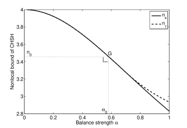
Figure 1: Relations between nonlocality upper bound and the balance strength $\alpha$. i) Balance relation imposes a constraint on non-locality, and the non-local bounds are given as functions of balance strength: the dash line $n_{\gamma}$ ($\alpha\leq 1$) represents the bound obtained under unbias assumption; the solid line $n_{s}$ represents the bound obtained with the unbias assumption and the symmetry assumption; ii) Non-locality also imposes a constraint on balance strength: the point $G$ shows that the balance strength of a theory which has exhibited correlation strength $n_{0}$ should be no greater than $\alpha_{0}$.

Taking into account the fact that QM has a unit balance strength, i.e., $\alpha_{\rm qm}=1$, one can readily reproduce Tsirelson bound from the upper bound Eq.(15). We note that without the additional symmetry assumption any theory with unite balance strength would have a nonlocality upper-bound of $n_{\gamma,\tau}=2.93$.

On the other hand, if the non-local bound of one theory is found to be $n_{0}$ as shown by the point $G$ in Fig.1, i.e., the maximal violation to CHSH inequality is $n_{0}$, then the corresponding balance strength of the given theory should be no greater than $\alpha_{0}$. If $\gamma=0$ assumption is taken again and from Eq.(15) we obtain the following constraint of balance strength by nonlocality

$$\alpha_{s}\leq\frac{\sqrt{16-n^{2}_{0}}}{n_{0}}.$$ (16)

Conclusion — We have introduced an uncertainty-complementarity balance relation, based on which we build connections among non-locality, uncertainty, and complementarity. Our considerations proceed without referring to any specific physical theory except the unbias assumption. Therefore our results hold generally and can be used to specify nonlocal theories. As applications, we explain QM non-locality and the PR-box non-locality with their balance relations, respectively.

Acknowledgement — This work has been supported by the Chinese Academy of Sciences, the National Natural Science Foundation of China under Grant No. 61125502, and the National Fundamental Research Program under Grant No. 2011CB921300.

I Supplementary Material

Proof of balance relation Eq.(4) for QM— Suppose that a quantum mechanical system is prepared in the state $\rho$ and after an ideal Von Neumann measurement $\{\hat{P}_{j|A}=|a_{j}\rangle\langle a_{j}|\}$ is performed the system is brought into a completely decohered state $\rho_{A}$ in the $A$ basis. Denoting by $\{\hat{P}_{i|A^{\prime}}\}$ the measurement of $A^{\prime}$, we have

$$D_{A\rightarrow A^{\prime}} = \sum_{i}|\operatorname{Tr}(\rho-\rho_{A})\hat{P}_{i|A^{\prime}}|$$ (17)

$$\leq \operatorname{Tr}|\rho-\rho_{A}|=\operatorname{Tr}\left|\textstyle\sum_{i<j}\sigma_{ij}\right|$$

$$\leq \sum_{i<j}\operatorname{Tr}|\sigma_{ij}|=\sum_{i<j}2|\langle a_{i}|\rho|a_{j}\rangle|$$

$$\leq \sum_{i<j}2\sqrt{p_{i|A}p_{j|A}}=\delta_{A}$$

where $\operatorname{Tr}|X|:=\operatorname{Tr}\sqrt{X^{\dagger}X}$ and $\sigma_{ij}:=|a_{i}\rangle\langle a_{i}|\rho|a_{j}\rangle\langle a_{j}|+|a_{j}\rangle\langle a_{j}|\rho|a_{i}\rangle\langle a_{i}|$ for $i\not=j$. In the above proof, we have used the convexity of trace-norm in the second line.

Proof the Balance strength $\alpha_{pr}=0$ for PR-box — Consider PR-box shared by Alice and Bob, by each measurement $B_{\mu}$ and outcome $b$ on Bob’s side he would prepare a conditional state $\omega_{b|B_{\mu}}$ on Alice’s side. By the non-signaling principle, Alice cannot confirm which conditional state is prepared in her hand by local operation. Consider one case that Alice has obtained an outcome $a=0$ by measuring $A_{0}$ (output state would then be brought into $\mathcal{S}_{0|A_{0}}$), she would know the measured state is either $\omega_{0|B_{0}}$ or $\omega_{0|B_{1}}$.

By $p(i|A_{1},\mathcal{S}_{0|A_{0}})$ and $p(i|A_{1},\omega_{0|B_{0}})$ we denote the probabilities of obtaining $i$ when measuring $A_{1}$ on $\mathcal{S}_{0|A_{0}}$ and on $\omega_{0|B_{0}}$. Following the definition of PR-box $p(1|A_{1},\omega_{0|B_{0}})=0,p(0|A_{1},\omega_{0|B_{0}})=1$, then disturbance $D_{A_{0}\rightarrow A_{1}}$ for $\omega_{0|B_{0}}$ is

$$D_{A_{0}\rightarrow A_{1}}(\omega_{0|B_{0}}) = \sum_{i}|p({i|A_{1}},\omega_{0|B_{0}})-p(i|A_{1},\mathcal{S}_{0|A_{0}})|$$

$$= 2(1-p(0|A_{1},\mathcal{S}_{0|A_{0}})).$$

Similarly, $D_{A\rightarrow A_{1}}(\omega_{0|B_{1}})=2p(0|A_{1},\mathcal{S}_{0|A_{0}})$, then

$$\sum_{i}D_{A_{0}\rightarrow A_{1}}(\omega_{0|B_{i}})=2.$$

By the definition of the box we have

$$\sum_{i}\delta A_{0}(\omega_{0|B_{i}})=0.$$

Following the general balance relation we have

$$\sum_{i}\delta A_{0}(\omega_{0|B_{i}})\geq\alpha_{pr}\sum_{i}D_{A_{0}\rightarrow A_{1}}(\omega_{0|B_{i}}).$$

Thus, $\alpha_{pr}=0$.

Proof of nonlocality upper bound Eq.(9)— From the normalization conditions such as $\sum_{i}P({i}|A_{1},\mathcal{S}_{\mu|A_{0}})=1$ and the unbias assumption Eq.(8) for two sequential measurements $A_{0}$ and $A_{1}$ there is only two independent parameters, e.g., $\gamma$ and $\tau$ as given in Eq.(11), among 4 probability distributions $\{P({i}|A_{\nu},\mathcal{S}_{\mu|A_{1-\nu}})\}$ with $\mu,\nu=0,1$. The disturbance reads

$$D_{A_{\mu}\to A_{\bar{\mu}}} = \sum_{a=0}^{1}\big{|}p({a|A_{\bar{\mu}}})-p({a|A_{\mu}\to A_{\bar{\mu}}})\big{|}$$

$$= 2\big{|}p({1|A_{\bar{\mu}}})-p({1|A_{\mu}\to A_{\bar{\mu}}})\big{|}$$

$$= 2\big{|}p({1|A_{\bar{\mu}}})-\textstyle\sum_{a}p({a|A_{\mu}})P(1|A_{\bar{\mu}},\mathcal{S}_{a|A_{\mu}})\big{|}$$

$$= \big{|}2p({1|A_{\mu}})-1+\gamma_{\mu}\overline{A}_{\bar{\mu}}\big{|}$$

$$= \big{|}\overline{A}_{\mu}+\gamma_{\mu}\overline{A}_{\bar{\mu}}\big{|}$$

with $\mu=0,1$, $\bar{\mu}=1-\mu$, and

$$\gamma_{\mu}=P(1|A_{\mu},\mathcal{S}_{0|A_{\bar{\mu}}})-P(1|A_{\mu},\mathcal{S}_{1|A_{\bar{\mu}}}).$$

The first equality is the definition of disturbance; the second equality is due to the normalization of probability distributions; the third equality is the definition of $P_{a|A_{\mu}\to A_{\bar{\mu}}}$ as in Eq.(3); the fourth equality follows from the unbias assumption with $\gamma_{0}=\gamma$ and $\gamma_{1}=\tau$ as defined in Eq.(11); in the last equality we have used $\bar{A}_{\mu}=p({0|A_{\mu}})-p({1|A_{\mu}})$. As a result we have

$$\sqrt{1-\overline{A}_{\mu}^{2}}=\delta_{A_{\mu}}\geq\alpha D_{A_{\mu}\to A_{\bar{\mu}}}=\alpha\big{|}\overline{A}_{\mu}+\gamma_{\mu}\overline{A}_{\bar{\mu}}\big{|}$$ (18)

with $\mu=0,1$. Squaring Eq.(18) and denoting $a=\overline{A}_{0}+\overline{A}_{1}$, $b=\overline{A}_{0}-\overline{A}_{1}$, we have

$$4\geq a^{2}(\alpha^{2}(1+\gamma)^{2}+1)+b^{2}(\alpha^{2}(1-\gamma)^{2}+1)$$

$$+2ab(\alpha^{2}(\gamma^{2}-1)+1)$$ (19)

$$4\geq a^{2}(\alpha^{2}(1+\tau)^{2}+1)+b^{2}(\alpha^{2}(1-\tau)^{2}+1)$$

$$-2ab(\alpha^{2}(\tau^{2}-1)+1)$$ (20)

from which we obtain, by eliminating $ab$ terms,

$$4\geq\frac{a^{2}}{f(\alpha,\gamma,\tau)}+\frac{b^{2}}{f(\alpha,-\gamma,-\tau)}$$ (21)

with $f(\alpha,\gamma,\tau)$ given by Eq.(10). As a result it holds

$$|\overline{A}_{0}\pm\overline{A}_{1}|\leq 2\sqrt{f(\alpha,\pm\gamma,\pm\tau)}$$ (22)

for any state of the subsystem in Alice’s hand. We note that after Bob’s measurement $B_{\nu}$ with outcome $b$ Alice’s subsystem will be brought into some state $\mathcal{S}_{b|\nu}$ with probability $p({b|B_{\nu}})$ so that

$$p(a,b|A_{\mu},B_{\nu})=p({b|B_{\nu}})p(a|A_{\mu},\mathcal{S}_{b|\nu}).$$

Denoting $\overline{A}_{\mu}(\mathcal{S}_{b|\nu})=\sum_{a}(-1)^{a}p(a|A_{\mu},\mathcal{S}_{b|\nu})$ we have

$$\operatorname{CHSH} =\sum_{a,b,\mu,\nu=0}^{1}(-1)^{a+b+\mu\nu}p(a,b|A_{\mu},B_{\nu})$$

$$\leq\sum_{b,\nu=0}^{1}p(b|B_{\nu})\left|\overline{A}_{0}(\mathcal{S}_{b|\nu})+(-1)^{\nu}\overline{A}_{1}(\mathcal{S}_{b|\nu})\right|$$

$$\leq\sum_{b,\nu=0}^{1}p(b|B_{\nu})2\sqrt{f(\alpha,(-1)^{\nu}\gamma,(-1)^{\nu}\tau)}$$

$$=2\sqrt{f(\alpha,\gamma,\tau)}+2\sqrt{f(\alpha,-\gamma,-\tau)}$$ (23)

where the second inequality is due to Eq.(22).

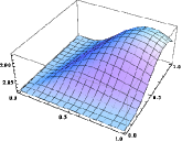
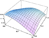
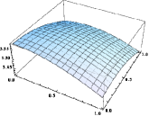
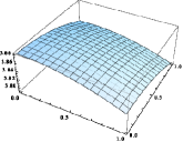
Figure 2: (Color online) The nonlocality upper bound $n_{\gamma\tau}$ is plotted as the function of $\gamma$ and $\tau$ with $\alpha=1$ (upper left), $\alpha=3/4$ (upper right), $\alpha=1/2$ (lower left), and $\alpha=1/4$ (lower right). We see clearly that the maximum is always attained at $\gamma=\tau$.

References

- (1) M. J. W. Hall. Local deterministic model of singlet state correlations based on relaxing measurement independence. Phys. Rev. Lett. 105, 250404 (2010).
- (2) R. W. Spekkens. Evidence for the epistemic view of quantum states: A toy theory. Phys. Rev. A 75, 032110 (2007).
- (3) G. Chiribella, G. M. DAriano, and Paolo Perinotti, Informational derivation of quantum theory, Phys. Rev. A 84, 012311 (2011).
- (4) L. Hardy. Quantum Theory From Five Reasonable Axioms. arXiv:quant-ph/0101012 (2001).
- (5) P. Janotta, and H. Hinrichsen. Generalized probability theories: what determines the structure of quantum theory? J. Phys. A: Math. Theor. 47, 323001 (2014).
- (6) H. Barnum, J. Barrett, M. Leifer, and A. Wilce. Generalized No-Broadcasting Theorem. Phys. Rev. Lett. 99, 240501 (2007).
- (7) Li. Masanes, A. Acin, and N. Gisin. General properties of nonsignaling theories. Phys. Rev. A 73, 012112 (2006).
- (8) J. Barrett. Information processing in generalized probabilistic theories. Phys. Rev. A 75, 032304 (2007).
- (9) S. Popescu. Nonlocality beyond quantum mechanics. Nature Phys, 10, 264 (2014).
- (10) B. Dakic, and C. Brukner. Quantum Theory and Beyond: Is Entanglement Special? arxiv:quant-ph/0911.0695, (2009).
- (11) R. Clifton, J. Bub, and H. Halvorson. Characterizing Quantum Theory in Terms of Information-Theoretic Constraints. Found. Phys 11 33 (2003).
- (12) N. Brunner, D. Cavalcanti, S. Pironio, V. Scarani, and S. Wehner. Bell nonlocality. Rev. Mod. Phys. 86, 419 (2014).
- (13) M. ukowski, A. Zeilinger, M. A. Horne, and Ekert. A. K. "Event-ready-detectors" Bell experiment via entanglement swapping Phys. Rev. Lett. 71, 4287 (1993).
- (14) A. J. Short, S. Popescu, and N. Gisin, Entanglement swapping for generalized nonlocal correlations. Phys. Rev. A 73, 012101 (2006).
- (15) G. Chiribella, G.M.D’Ariano, P. Perinotti. Probabilistic theories with purification. Phys. Rev. A, 81 062348 (2010).
- (16) Liang-Liang Sun, Fei-Lei Xiong, Sixia Yu, Zeng-Bing Chen, Theory-Independent Measure of Coherence, arxiv:quant-ph/1705.01044v2, (2018).
- (17) H. Barnum, J. Barrett, M. Leifer, and A. Wilce, Teleportation in General Probabilistic Theories. arxiv:quant-ph/0805.3553.
- (18) S. Popescu and D, Rohirlich. Quantum nonlocality as an axiom. Found. Phys. 24 379 (1994).
- (19) J. Oppenheim, and S. Wehner. The uncertainty principle determines the non-locality of quantum mechanics. Science 330,1072 (2010).
- (20) J. odyga, W. K obus, R. Ramanathan, A. Grudka, M. Horodecki, and R. Horodecki. Measurement uncertainty from no-signaling and nonlocality. Phys. Rev. A 96, 012124 (2017).
- (21) M. Pawlowski, T. Paterek, D. Kaszlikowski, V. Scarani, A. Winter, and M. Zukowski. Information Causality as a Physical Principle. Nature 461, 1101 (2009).
- (22) W. van Dam. Implausible consequences of superstrong nonlocality. Nat. Comput 12:9-12 (2013).
- (23) A. Cabello. Simple Explanation of the Quantum Violation of a Fundamental Inequality. Phys. Rev. Lett. 110, 060402 (2013).
- (24) B. Yan. Quantum Correlations are Tightly Bound by the Exclusivity Principle. Phys. Rev. Lett. 110, 260406 (2013).
- (25) A. Cabello. Quantum Correlations are Tightly Bound by the Exclusivity Principle. Phys. Rev. A 90, 062125 (2014).
- (26) M. Kleinmann. Sequences of projective measurements in generalized probabilistic models. J. Phys. A: Math. Theor. 47, 455304 (2014).
- (27) G. Chiribella, X.Yuan. Measurement sharpness cuts nonlocality and contextuality in every physical theory. arXiv:quant 1404.3348 (2014).
- (28) P. Busch, P. Lahti, and R. F. Werner. Colloquium: Quantum root-mean-square error and measurement uncertainty relations. Rev. Mod. Phys. 86, 1261 (2014).
- (29) L. D. Landau and E. M. Lifshitz, Quantum Mechanics, 2nd ed., translated from Russian by J. B. Sykes and J. S. Bell (Pergamon, New York, 1965), Vol. 3.
- (30) R. W. Spekkens, Evidence for the epistemic view of quantum states: A toy theory, Phys. Rev. A 75, 032110 (2007).
- (31) J. J. Sakurai, Modern Quantum Mechanics, edited by S. F. Tuan (Addison-Wesley, Reading, MA, 1994).
- (32) P. Busch, P. Lahti, and R. F. Werner. Colloquium: Quantum root-mean-square error and measurement uncertainty relations. Rev. Mod. Phys. 86, 1261 (2014).
- (33) M. A. Nielsen and I. L. Chuang, Quantum Computation and Quantum Information (Cambridge University Press, Cambridge, UK, 2000).