Jiamusi Pulsar Observations: II. Scintillations of 10 Pulsars

Abstract

Context. Pulsars scintillate. Dynamic spectra show brightness variation of pulsars in the time and frequency domain. Secondary spectra demonstrate the distribution of fluctuation power in the dynamic spectra.

Aims. Dynamic spectra strongly depend on observational frequencies, but were often observed at frequencies lower than 1.5 GHz. Scintillation observations at higher frequencies help to constrain the turbulence feature of the interstellar medium over a wide frequency range and can detect the scintillations of more distant pulsars.

Methods. Ten pulsars were observed at 2250 MHz (S-band) with the Jiamusi 66 m telescope to study their scintillations. Their dynamic spectra were first obtained, from which the decorrelation bandwidths and time scales of diffractive scintillation were then derived by autocorrelation. Secondary spectra were calculated by forming the Fourier power spectra of the dynamic spectra.

Results. Most of the newly obtained dynamic spectra are at the highest frequency or have the longest time span of any published data for these pulsars. For PSRs B0540+23, B2324+60 and B2351+61, these were the first dynamic spectra ever reported. The frequency-dependence of scintillation parameters indicates that the intervening medium can rarely be ideally turbulent with a Kolmogorov spectrum. The thin screen model worked well at S-band for the scintillation of PSR B1933+16. Parabolic arcs were detected in the secondary spectra of three pulsars, PSRs B0355+54, B0540+23 and B2154+40, all of which were asymmetrically distributed. The inverted arclets of PSR B0355+54 were seen to evolve along the main parabola within a continuous observing session of 12 hours, from which the angular velocity of the pulsar was estimated that was consistent with the measurement by very long baseline interferometry (VLBI).

1 INTRODUCTION

Pulsars are radio point sources and often move at high speeds of a few tens to more than a thousand km s^-1. When radio signals from pulsars propagate through the interstellar medium, they are scattered due to irregularly distributed thermal electrons. The scattering due to the small scale irregularities of the medium can cause not only the delayed arrival of the scattered radiation, shown as larger temporal broadening of pulse profiles at lower frequencies, but also angular broadening for the scattering disk of a pulsar image that can be observed by VLBI. The random electron density fluctuations in the interstellar medium can be quantitatively described by a power spectrum of $P(k)=C_{n}^{2}k^{-\beta}$ in a given spatial scale range of $L$ for $k=2\pi/L$ in a given interstellar region (Armstrong et al. 1995); here, $C_{n}^{2}$ is a measure of fluctuations. A Kolmogorov spectrum with $\beta\simeq 11/3$ is widely used to describe the turbulent medium. Nevertheless, the electron density fluctuations in the interstellar medium, at least in some regions, do not follow the Kolmogorov spectrum and may have a different spectral index $\beta$ (e.g. Spangler & Gwinn 1990; Bhat et al. 1999c).

Table 1: Parameters of 10 pulsars are listed together with frequencies for previous dynamic spectrum observations.

PSRs	Period	DM	$l$	$b$	$z$	Distance	$V_{\rm p}$	Freq. of Prev. Obs. (ref. Table 2)
	(s)	(pc cm-3)	(∘)	(∘)	(kpc)	(kpc)	$(\rm km\leavevmode\nobreak\ s^{-1})$	$\nu$ ¡ 2.3 (GHz)	$\nu\geq$ 2.3 (GHz)
B0329$+$54	0.714	26.76	145.00	$-$1.22	$-$0.02	1.0(1)d	95(12)a	0.327, 0.408, 0.61	-
								0.96, 1.42, 1.54
B0355$+$54	0.156	57.14	148.19	0.81	0.01	1.0(2)d	61(12)b	0.325, 0.96	-
B0540$+$23	0.245	77.70	184.36	$-$3.32	$-$0.09	1.6(2†)e	166(25†)f	-	-
B0740$-$28	0.166	73.78	243.77	$-$2.44	$-$0.09	2(1)d	277(42†)f	-	4.8, 8.4
B1508$+$55	0.739	19.61	91.33	52.29	1.66	2.1(1)d	963(64)c	0.327,0.408	-
B1933$+$16	0.358	158.52	52.44	$-$2.09	$-$0.14	3.7(13)d	394(208)c	1.67	-
B2154$+$40	1.525	71.12	90.49	$-$11.34	$-$0.57	2.9(5)d	264(73)c	1.42	-
B2310$+$42	0.349	17.27	104.41	$-$16.42	$-$0.30	1.06(8)d	125(10)c	0.327	-
B2324$+$60	0.233	122.61	112.95	0.00	0.00	2.7(4†)e	245(37†)f	-	-
B2351$+$61	0.944	94.66	116.24	$-$0.19	$-$0.01	2.4(4†)e	259(39†)f	-	-

A moving pulsar with a transverse velocity of $V_{\rm p}$ shines through the relatively stable interstellar medium with small scale irregularities of 10^6-8 cm causing diffractive scintillation. This is exhibited by rapid fluctuations in time and radio frequency in a dynamic spectrum. The typical time-scale, $\Delta t_{d}$, and decorrelation bandwidth, $\Delta\nu_{d}$, depend on observation frequency $\nu$ and the amount of intervening medium indicated by $\rm DM$ or roughly by pulsar distance $D$, in the form of (see Rickett 1977; Wang et al. 2005)

$$\Delta t_{d}\propto\nu^{6/5}D^{-3/5}V_{\rm s}^{-1},\\ \Delta\nu_{d}\propto\nu^{22/5}D^{-11/5}.$$ (1)

Here $V_{\rm s}$ is the speed of scintillation pattern past the observer, which is caused by the velocities of the source and the Earth as well as the intervening medium, and has often been used to estimate the pulsar velocity $V_{\rm p}$ assuming other velocities are negligible. The scintillation speed $V_{\rm s}$ can be estimated from $\Delta t_{d}$, $\Delta\nu_{d}$ and pulsar distance $D$ by (Lyne & Smith 1982; Cordes 1986; Gupta 1995),

$$V_{\rm s}=A\left(\frac{D}{\rm kpc}\right)^{1/2}\left(\frac{\Delta\nu_{d}}{\rm MHz}\right)^{1/2}\left(\frac{\nu}{\rm GHz}\right)^{-1}\left(\frac{\Delta t_{d}}{\rm s}\right)^{-1},$$ (2)

assuming a thin scattering screen. The constant $A$, depending on the screen location and the form of the turbulence spectrum, was found to be $A=3.85\times 10^{4}\leavevmode\nobreak\ \rm km\leavevmode\nobreak\ s^{-1}$ (Gupta 1995) for a screen located at a half way between the pulsar and the observer. The scintillation strength, $u$, originally defined as the ratio of the Fresnel scale $s_{F}$ with respect to the field coherence scale $s_{0}$ (i.e, $u=s_{F}/s_{0}$, see Rickett 1990), can be estimated from the observation frequency $\nu$ and the decorrelation bandwidth $\Delta\nu_{d}$ by

$$u\simeq\left(\frac{\nu}{\Delta\nu_{d}}\right)^{0.5}.$$ (3)

The fluctuation measure $C_{n}^{2}$ can be estimated from $\nu$, $\Delta\nu_{d}$ and pulsar distance $D$ by (Cordes et al. 1985)

$$C_{n}^{2}\approx 0.002\;\nu^{11/3}D^{-11/6}\Delta\nu_{d}^{-5/6}$$ (4)

for the Kolmogorov case. When the interstellar medium has a different fluctuation power-law spectrum, i.e. different index $\beta$, these above scaling relations could be different (Romani et al. 1986; Rickett 1990; Bhat et al. 1999c).

When pulsar signals propagate through large-scale irregular clouds of 10^10-12 cm with various electron density distributions, refractive scintillation can be observed as pulsar flux density fluctuations on longer time scales in addition to small-amplitude intensity variations (Rickett et al. 1984). Refraction moves scintillation pattern laterally and causes its systematic drift, which is manifested as fringes on pulsar dynamic spectra. The slope of the fringes is (e.g. Smith & Wright 1985; Bhat et al. 1999c)

$$\frac{{\rm d}t}{{\rm d}\nu}\simeq\frac{D\theta_{r}}{V_{\rm s}}\frac{1}{\nu},$$ (5)

where $\theta_{r}$ is the refractive angle which is approximately proportional to $\nu^{-2}$ for a given gradient of refractive index.

Previously, scintillations of more than 80 pulsars have been observed mostly at lower frequencies (e.g. Lyne & Smith 1982; Roberts & Ables 1982; Smith & Wright 1985; Balasubramanian & Krishnamohan 1985; Cordes et al. 1985; Cordes 1986; Cordes & Wolszczan 1986; Gupta et al. 1994; Malofeev et al. 1996; Bhat et al. 1999b; Gothoskar & Gupta 2000; Wang et al. 2005). For a given pulsar, the decorrelation bandwidth $\Delta\nu_{d}$ and scintillation time-scale $\Delta t_{d}$ are closely related to observation frequenciess (e.g. Cordes et al. 1985). Such observed frequency dependencies can be used to estimate the power-law index $\beta$ for electron density fluctuations in the interstellar medium, which has often been found to deviate from the Kolmogorov spectrum (Gupta et al. 1994; Bhat et al. 1999c; Wang et al. 2005).

Table 2: Previous observations of the 10 pulsars for scintillation parameters.

PSRs	Freq.	$\Delta\nu_{d}$	$\Delta t_{d}$	Reference	PSRs	Freq.	$\Delta\nu_{d}$	$\Delta t_{d}$	Reference
	(MHz)	(MHz)	(min)			(MHz)	(MHz)	(min)
B0329$+$54	327	0.165	5.12	Bhat et al. (1999b)	B0540$+$23	430	0.0019	-	Cordes et al. (1985)
	327	0.02†	-	Wolszczan (1983)		1380	0.150	-	Cordes et al. (1985)
	330	0.016†	-	Wolszczan et al. (1981)		1410	0.31	-	Cordes et al. (1985)
	340	0.023†	-	Armstrong & Rickett (1981)		1420	0.28	-	Cordes et al. (1985)
	408	0.047	3.23	Gupta et al. (1994)		1420	0.317	-	Cordes et al. (1985)
	408	0.083	4.5	Lyne & Smith (1982)		4750	-	8	Malofeev et al. (1996)
	410	0.056†	-	Armstrong & Rickett (1981)		10550	-	8	Malofeev et al. (1996)
	410	0.07†	-	Rickett (1970)	B0740$-$28	660	-	0.97	Johnston et al. (1998)
	410	0.100	-	Rickett (1977)		4750	-	5	Malofeev et al. (1996)
	480	0.103	-	Wolszczan (1983)		4800	8.83	10.63	Johnston et al. (1998)
	610	0.13	4.43	Safutdinov et al. (2017)		8400	40.0	37.67	Johnston et al. (1998)
	610	0.22	5.34	Safutdinov et al. (2017)		10550	-	3.5	Malofeev et al. (1996)
	610	0.348†	-	Rickett (1970)	B1508$+$55	327	0.168	2.63	Bhat et al. (1999b)
	610	0.349	5.90	Stinebring et al. (1996)		327	0.226	2.73	Bhat et al. (1999b)
	960	0.92	12.94	Smith & Wright (1985)		340	0.139†	-	Armstrong & Rickett (1981)
	1410	2	-	Wolszczan et al. (1974)		408	0.8	3	Smith & Wright (1985)
	1420	5.93	15.52	Safutdinov et al. (2017)		408	1.67	-	Lyne & Smith (1982)
	1540	14	16.9	Wang et al. (2005)		410	0.13†	-	Rickett (1970)
	1540	9.2	17.1	Wang et al. (2008)		930	-	1.35	Lyne & Smith (1982)
	4750	-	21	Malofeev et al. (1996)	B1933$+$16	1410	0.125	-	Wolszczan et al. (1974)
	4800	-	42.7	Lewandowski et al. (2011)		1416	0.037†	-	Wolszczan (1983)
	10550	-	23	Malofeev et al. (1996)		1420	0.1	-	Rickett (1977)
B0355$+$54	325	0.06	1.01	Safutdinov et al. (2017)		1670	0.110	0.75	Roberts & Ables (1982)
	408	-	1.83	Lyne & Smith (1982)	B2154$+$40	1000	0.195	0.503	Cordes (1986)
	410	0.018†	-	Armstrong & Rickett (1981)		1420	0.20	0.55	Safutdinov et al. (2017)
	930	0.765	-	Lyne & Smith (1982)	B2310$+$42	327	0.114	5.15	Bhat et al. (1999b)
	960	0.613	4.31	Smith & Wright (1985)	B2324$+$60	-	-	-	-
	1410	0.575	-	Wolszczan et al. (1974)	B2351$+$61	10550	-	15	Malofeev et al. (1996)
	4750	-	12.5	Malofeev et al. (1996)
	10550	-	13.5	Malofeev et al. (1996)

When a high-sensitivity dynamic spectrum of a pulsar is obtained, not only strong large patterns in time and bandwidth are observed; but also faint organized structures on smaller scales may appear in the dynamic spectrum image. These are best studied through the secondary spectrum, which is the power spectrum of the dynamic spectrum; i.e. $S_{2}(f_{t},f_{\nu})=|\tilde{S_{1}}(t,\nu)|^{2}$, where $S_{1}$ is the dynamic spectrum and the tilde indicates a Fourier transform. Assuming that the pulsar velocity dominates and that any linear scattering structure is aligned along the effective velocity vector, one can estimate the fractional distance $d$ of the intervening screen from a pulsar at the distance $D$ with a velocity $V_{\rm p}$ based on the curvature of the arc in the secondary spectrum via (see e.g. Cordes et al. 2006)

$$f_{\nu}=\frac{\lambda^{2}D}{2cV_{\rm p}^{2}}\left(\frac{d}{1-d}\right)f_{t}^{2},$$ (6)

here, $f_{t}=1/t$ is the conjugate time, $f_{\nu}=1/\nu$ is conjugate frequency, $\lambda$ is the observing wavelength, $c$ is the speed of light. The curvature of a primary arc in the $f_{t}$ and $f_{\nu}$ plane is

$$\Omega=\frac{\lambda^{2}D}{2cV_{\rm p}^{2}}\left(\frac{d}{1-d}\right).$$ (7)

Previously, such arcs in the secondary spectra have been detected for only 13 pulsars: PSRs B1133+16 (Cordes & Wolszczan 1986; Stinebring et al. 2001; Hill et al. 2003), B0823+26, B0834+06 (Stinebring et al. 2001; Hill et al. 2003), B0919+06 and B1929+10 (Stinebring et al. 2001; Hill et al. 2003; Stinebring 2007), J0737$-$3039 (Stinebring et al. 2005), B1737+13 (Cordes et al. 2006; Stinebring 2007), B0355+54 (Stinebring 2007; Xu et al. 2018), J0437$-$4715 (Bhat et al. 2016), B1642$-$03, B1556$-$44, B2021+51 and B2154+40 (Safutdinov et al. 2017). The placements of the intervening screen have so been estimated.

In this paper, we present the scintillation observations of ten pulsars using the Jiamusi 66-m telescope at 2250 MHz. Parameters of these pulsars are listed in Table 1, and previous scintillation observations are given in Table 2. The dynamic spectra presented in this paper are valuable supplements to the previous observations and, in some cases, are the first dynamic and secondary spectra ever published. In Section 2 we describe our observation system. Observational results are presented and analyzed in Section 3. Discussion and conclusions are given in Sections 4 and 5, respectively.

Table 3: Observational parameters and derived scintillation parameters, with uncertainties for the last digit given in brackets.

PSR name	Date	MJD	chW	$\rm\delta t$	$T_{\rm obs}$	$\Delta\nu_{d}$	$\Delta t_{d}$	${\rm d}t/{\rm d}\nu$	$u$	log $C_{n}^{2}$	$V_{\rm s}$
			(MHz)	(s)	(min)	(MHz)	(min)	(min/MHz)		$(\rm m^{-20/3})$	$(\rm km\leavevmode\nobreak\ s^{-1})$
B0329$+$54	2016/02/21	57439.103	0.58	30	306	17(2)	19(2)	-0.09(1)	12(1)	-2.43(10)	62(7)
	2016/02/24	57442.227	0.58	30	426	20(2)	26(3)	-0.39(5)	11(1)	-2.49(8)	49(6)
	2017/11/08	58065.445	0.58	30	655	67(14)	30(6)	0.02(1)	6(1)	-2.93(17)	78(18)
B0355$+$54	2015/08/20	57254.546	0.58	30	654	15(1)	9(1)	0.18(1)	12(1)	-2.39(4)	123(14)
	2016/01/29a	57416.036	0.58	30	720	4.0(1)	2.4(1)	-0.39(1)	24(1)	-1.91(2)	238(10)
	2016/01/29b	57416.556	0.58	30	96	4.3(2)	2.9(1)	-0.35(2)	23(1)	-1.94(4)	204(8)
	2017/11/05	58062.678	0.58	30	486	41(5)	13(2)	-0.23(2)	8(1)	-2.75(10)	140(23)
	2017/11/09	58066.421	0.58	30	362	22(2)	7(1)	-0.16(1)	10(1)	-2.53(8)	191(29)
B0540$+$23	2015/06/25	57198.154	0.58	30	50	1.9(1)	2.9(1)	0.95(5)	35(1)	-1.99(4)	169(7)
	2016/08/08	57608.863	0.58	30	168	2.3(1)	2.5(1)	0.53(4)	32(1)	-2.06(4)	216(10)
	2017/11/01	58058.549	0.58	30	336	1.3(1)	2.6(1)	0.30(2)	42(2)	-1.86(6)	156(8)
B0740$-$28	2015/12/12	57368.687	0.58	30	168	1.1(1)	5.2(2)	-0.05(12)	45(2)	-1.99(8)	81(5)
	2016/01/26	57413.544	1.17	30	186	1.1(1)	2.9(1)	0.20(14)	45(2)	-1.99(8)	146(8)
	2017/11/01	58058.793	0.58	30	156	0.6(1)	3.0(1)	-0.54(19)	61(5)	-1.77(14)	104(9)
B1508$+$55	2015/12/13	57369.830	0.58	60	138	8.1(5)	3.2(2)	-0.20(1)	17(1)	-2.76(5)	368(26)
	2017/10/31	58057.067	0.58	60	67	44(8)	4(1)	-0.03(1)	8(1)	-3.37(15)	685(182)
B1933$+$16	2015/06/15	57188.756	0.58	30	31	1.36(6)	2.35(9)	0.74(5)	41(1)	-2.56(4)	272(12)
	2016/02/18	57436.861	0.58	30	300	0.97(2)	1.60(5)	0.37(7)	48(1)	-2.44(2)	338(11)
	2016/02/25	57443.861	0.58	30	564	0.77(3)	1.37(6)	0.24(11)	54(1)	-2.35(1)	351(17)
	2016/05/20	57528.742	0.58	30	378	1.82(2)	2.03(2)	-0.26(2)	35(1)	-2.67(1)	365(4)
	2016/05/21	57529.629	0.58	30	540	1.67(1)	2.01(2)	-0.24(2)	37(1)	-2.63(1)	353(4)
	2016/05/22	57530.652	0.58	30	504	1.51(2)	2.03(2)	-0.39(2)	39(1)	-2.60(1)	332(4)
	2016/05/23	57531.730	0.58	30	389	1.79(2)	2.20(3)	-0.25(2)	36(1)	-2.66(1)	334(5)
	2016/05/25	57533.790	0.58	30	200	2.58(6)	2.61(6)	-0.16(2)	30(1)	-2.79(2)	338(9)
B2154$+$40	2016/01/25	57412.291	0.58	30	164	1.60(3)	1.42(3)	-0.26(2)	38(1)	-2.43(2)	433(10)
	2017/10/31	58057.533	0.58	30	276	2.34(5)	2.44(5)	-0.68(3)	31(1)	-2.56(2)	304(7)
	2017/11/10	58067.151	0.58	30	216	4.1(1)	2.41(7)	-0.27(2)	24(1)	-2.77(2)	408(13)
B2310$+$42	2015/07/20	57223.566	0.58	90	145	15(2)	13(2)	-0.51(7)	13(1)	-2.43(11)	87(15)
	2017/10/25	58051.568	0.58	30	360	35(6)	23(4)	-0.27(5)	8(1)	-2.74(14)	76(15)
B2324$+$60	2017/03/29	57841.268	0.58	60	187	2.3(1)	1.7(1)	0.13(2)	32(1)	-2.51(4)	420(26)
	2017/11/04	58061.117	0.58	60	346	2.2(1)	1.7(1)	0.33(2)	32(1)	-2.49(4)	411(26)
B2351$+$61	2015/06/18	57191.677	0.58	90	35	2.5(2)	2.6(2)	-0.38(2)	30(1)	-2.44(7)	269(23)
	2016/08/10	57610.886	0.58	90	150	6.0(3)	2.9(2)	0.15(1)	20(1)	-2.75(4)	373(27)

2 Observations and data processing

Observations of ten pulsars were carried out between 2015 June and 2017 November using the Jiamusi 66-m telescope at the Jiamusi Deep Space Station, China Xi’an Satellite Control Center. The observation system used here is the same as the one described in Han et al. (2016, see their figure 1 for the diagram). In short, the Jiamusi 66-m telescope is equipped with a cryogenically cooled dual-channel S-band receiver. We observed pulsars with this receiver at the central frequency of 2250 MHz with a bandwidth of about 140 MHz. The down-converted intermediate frequency signals from the receiver for the left and right hand polarizations were fed into a digital backend. The signals were sampled and then channelized by an FFT module in the digital backend. The total radio power from the two polarizations was then added for each of the 256 frequency channels with a channel width of 0.58 MHz. The data were saved to disk with a time resolution of 0.2 ms. Alternatively, 128 channels were sampled with a time resolution of 0.1 ms and with a channel width of 1.17 MHz. Observational parameters are listed in Table 3 for the ten pulsars.

Offline data processing includes several steps. First, radio frequency interference was manually identified from the two-dimensional plots of data on the frequency channel and time domain, and the affected data were simply excised. Second, the sampled total power data from every channel were re-scaled according to the observations of the flux-calibrators, 3C286 or 3C295. Third, data from each channel were then folded with the ephemerides of the pulsars, with a subintegration time of $\delta t=$ 30 s or 60 s or 90 s for a significant detection of pulse flux density. For each subintegration at each frequency channel, the flux density within the pulse window was calculated after subtracting a baseline offset and then normalized by the offset to form the dynamic spectrum, $S_{1}(t,\nu)$. During the analysis, software packages: DSPSR (van Straten & Bailes 2011) and PSRCHIVE (Hotan et al. 2004), were employed.

To obtain the auto-correlation function, the mean flux density $\langle S_{1}\rangle$ was first subtracted from the dynamic spectrum of each observation to get $\Delta S_{1}(t,\nu)=S_{1}(t,\nu)-\langle S_{1}\rangle$. Meanwhile, the previously excised pixels of the dynamic spectrum were interpolated by nearby samples. Then, the covariance function was computed (Cordes 1986; Wang et al. 2005):

$$\begin{split}&C_{f}(\Delta t,\Delta\nu)=N(\Delta t,\Delta\nu)^{-1}\times\\ &\sum_{j=1}^{N_{\nu}-N_{|\Delta\nu|}}\sum_{i=1}^{N_{t}-N_{|\Delta t|}}\Delta S(t_{i},\nu_{j})\Delta S(t_{i}+\Delta t,\nu_{j}+\Delta\nu).\end{split}$$ (8)

Here, $N_{\nu}$ and $N_{t}$ are the numbers of frequency channels and subintegrations respectively, $N_{|\Delta\nu|}$ and $N_{|\Delta t|}$ are the lags in the $\nu$ and $t$ directions, and $N(\Delta t,\Delta\nu)$ represents the number of pairs for the correlation pixels. Finally, the covariance function was normalized by its amplitude at zero lags to get the autocorrelation function

$$A(\Delta t,\Delta\nu)=\frac{C_{f}(\Delta t,\Delta\nu)}{C_{f}(0,0)}.$$ (9)

Since $C_{f}(0,0)$ contains a significant “noise” from interpolated dummy pixels, it was specially replaced by the peak value of the Gaussian function fitted to nearby points (see below).

The scintillation parameters were derived from the auto-correlation functions. Following Gupta et al. (1994), a two-dimensional elliptical Gaussian function in the form of

$$G(t,\nu)=C_{0}{\rm exp}[-(C_{1}\nu^{2}+C_{2}\nu t+C_{3}t^{2})]$$ (10)

was fitted to the main peak of $A(\Delta t,\Delta\nu)$ with $C_{0}$ fixed to unity. The decorrelation frequency, $\Delta\nu_{d}$, was measured from the fitted two-dimensional elliptical Gaussian function as the half width at the half maximum of $A(\Delta t,\Delta\nu)$, and the time scale, $\Delta t_{d}$, was measured as the half width for $A(\Delta t,\Delta\nu)$ to declined to $1/e$ (see Cordes 1986); hence, $\Delta\nu_{d}=(\ln 2/C_{1})^{0.5},$ $\Delta t_{d}=(1/C_{3})^{0.5},$ and the orientation of the elliptical Gaussian was given by ${{\rm d}t}/{{\rm d}\nu}=-C_{2}/(2C_{3}),$ see Bhat et al. (1999a). The so-deduced scintillation parameters for observations of the ten pulsars are listed in Table 3. Meanwhile, as noted in Bhat et al. (1999a), the uncertainties in $\Delta\nu_{d}$, $\Delta t_{d}$ and ${{\rm d}t}/{{\rm d}\nu}$ consist of not only the fitting uncertainty but also the statistical uncertainty caused by the finite number of independent scintles in the dynamic spectra. The fractional uncertainty of scintle statistics is given by

$$\sigma_{\rm est}=\left[f\left(\frac{B_{\rm obs}}{\Delta\nu_{d}}\frac{T_{\rm obs}}{\Delta t_{d}}\right)\right]^{-0.5},$$ (11)

here $B_{\rm obs}$ and $T_{\rm obs}$ represent the total observing bandwith and time, and the effective filling factor $f$ for the scintles is chosen to be $f=0.5$. In this paper, the fitting and statistical uncertainties were added in quadrature to derive the uncertainties of $\Delta\nu_{d}$, $\Delta t_{d}$ and ${{\rm d}t}/{{\rm d}\nu}$, and also derived parameters $u$, $C_{n}^{2}$ and $V_{\rm s}$, in Table 3, given in parentheses after each value.

The secondary spectrum was obtained by calculating the power spectrum of the dynamic spectrum through two-dimensional FFT. During our calculation, the dynamic spectra were first interpolated over the RFI affected pixels to reduce the leakage of power. The generalized Hough transform (see details in Bhat et al. 2016) together with fitting parabolas by eye were used to obtain the curvatures of the secondary spectra.

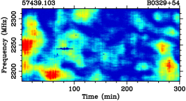
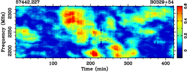
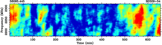
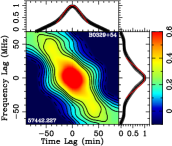
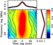
Figure 1: The dynamic spectra $S_{1}(t,\nu)$ from three observations of PSR B0329+54 (upper three panels) and their auto-correlation functions $A(\Delta t,\Delta\nu)$ (panels in the lowest rank). Some dummy points caused by the interference are set as $S_{1}(t,\nu)=0$. Observation time (in MJD) and pulsar name are indicated above each plot. The auto-correlation functions are plotted against time lag $\Delta t$ in minutes and frequency lag $\Delta\nu$ in MHz. The two-dimensional Gaussian functions are fitted to the main peaks of auto-correlation functions to derive the scintillation parameters. In the side-panels only data for the cross-sections are shown by “x” (too many for this pulsar as if a thick line, but not so many for other pulsars shown in other figures) and the fitted lines at $\Delta t=0$ and $\Delta\nu=0$ are drawn. The color schemes are indicated by the wedges for both the dynamic spectra and auto-correlation functions, which are saturated at $-10$% and 60% of the peak values (with exceptions for other pulsars but especially marked).

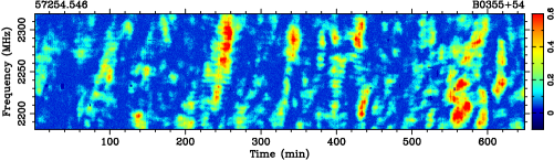
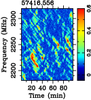
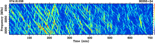
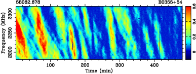
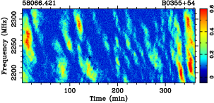
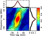
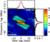
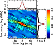
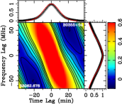
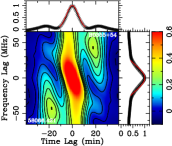
Figure 2: Dynamic spectra from five observations of PSR B0355+54 (upper five panels) and their autocorrelation functions (panels in the last rank). See keys in Fig. 1.

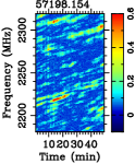
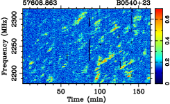
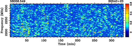
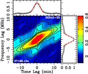
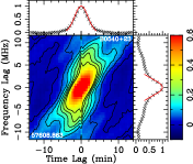
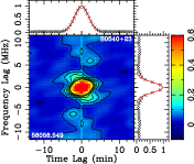
Figure 3: Dynamic spectra from three observations of PSR B0540+23 (upper panels) and their autocorrelation functions (lower panels) See keys in Fig. 1.

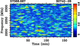
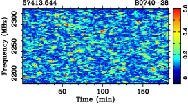
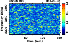
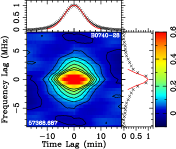
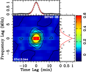
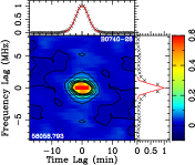
Figure 4: Dynamic spectra from three observations of PSR B0740-28 (upper panels) and their autocorrelation functions (lower panels). See keys in Fig. 1.

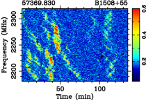
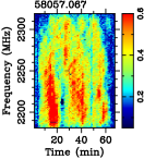
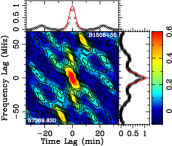
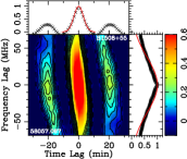
Figure 5: Dynamic spectra from two observations of PSR B1508+55 (upper two panels) and their autocorrelation functions (lower two panels). See keys in Fig. 1.

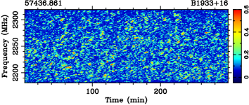
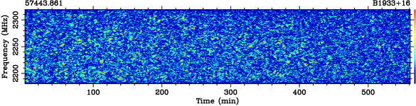
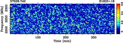
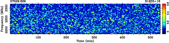
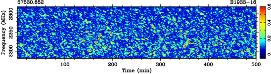
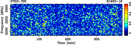
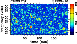
Figure 6: Dynamic spectra from eight observations of PSR B1933+16. See keys in Fig. 1.

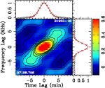
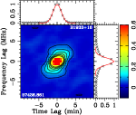
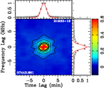
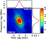
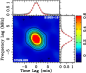
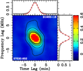
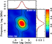
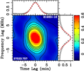
Figure 7: The autocorrelation functions of dynamic spectra for eight observations of PSR B1933+16. See keys in Fig. 1.

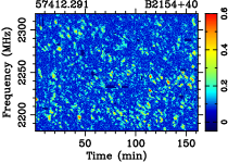
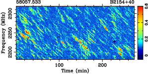
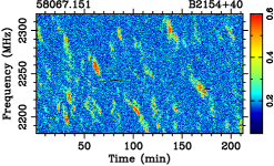
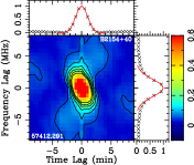
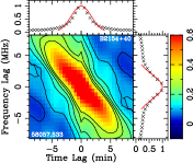
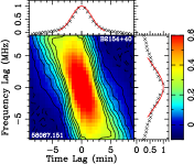
Figure 8: Dynamic spectra (upper three panels) and autocorrelation functions (bottom three panels) for three observations of PSR B2154+40. See keys in Fig. 1.

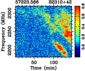
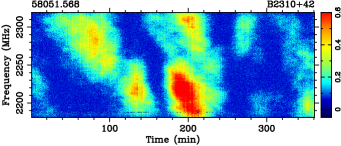
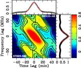
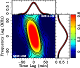
Figure 9: Dynamic spectra from two observations of PSR B2310+42 (upper two panels) and the autocorrelation functions (lower two panels). See keys in Fig. 1.

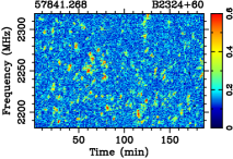
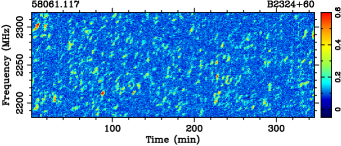
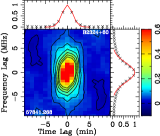
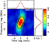
Figure 10: Dynamic spectra from two observations of PSR B2324+60 (upper two panels) and the autocorrelation functions (lower two panels). See keys in Fig. 1.

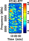
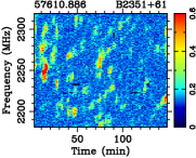
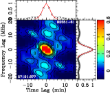
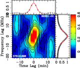
Figure 11: Dynamic spectra from two observations of PSR B2351+61 (upper panels) and the autocorrelation functions (lower panels). See keys in Fig. 1.

3 Dynamic spectra and derived scintillation parameters

In the following, we discuss scintillation observations for each pulsar.

3.1 PSR B0329+54

PSR B0329+54 is a bright pulsar in the northern sky. Its scintillation has been observed by many authors (see Table 2) in a range of frequencies from 327 MHz to more than 10 GHz. Though the decorrelation bandwidths and scintillation time scales have somehow different values from many observations even at one given band (e.g. Stinebring et al. 1996; Wang et al. 2008), the scintillation parameters clearly follow a power-law with observational frequencies (Cordes et al. 1985; Lewandowski et al. 2011), which will be discussed in Sect. 4.1.

We made three long observations at the S-band for 306, 426 and 655 minutes, respectively, and obtained their dynamic spectra (see Fig. 1) which were at the highest frequency currently available. Obviously, the scintles are of various scales in different sessions. We carefully inspected the intensity variations of individual pulses, and realized that the pulses were modulated and not so stable within a subintegration time of less than 30 s. The normalization for the subintegration by its own total power could reduce the modulation, but might distort the dynamic spectra. Hence, we got the mean pulse intensity for each channel with a subintegration time of $\rm\delta t=30$ s (or 60 s or 90 s for other pulsars, see Table 3) without normalization. The scintillation parameters are then derived from the auto-correlation functions. The scintillation time scale ranged from 19 to 30 minutes at the S-band (see Table 3). Long observations are thus necessary to get enough independent scintles in the dynamic spectra.

3.2 PSR B0355+54

PSR B0355+54 was previously observed for interstellar scintillation in the frequency range from 325 MHz to more than 10 GHz (see Table 2), and dynamic spectra were published by Wolszczan et al. (1974), Stinebring (2007) and recently by Xu et al. (2018).

We made five observations for this pulsar, one of which lasted for as long as 720 minutes. The new observations showed quite different dynamic spectra (see Fig. 2). The first observation at 57254 exhibited a wide-scintillation band and long time scale (see Table 3), so did the last two observations at 58062 and 58066. However, the two observations in the middle session at 57416 gave not only a much narrower scintillation band and finer time scale, but also fringes periodic in both frequency and time, and even with crossed fringes with different drifting rates in the dynamic spectra. These features were well-shown in the secondary spectra and would be further discussed in Sect.4.5.

The scintillation parameters (see Table 3) were also estimated from the newly observed dynamic spectra. The decorrelation bandwidth was at the highest frequency (see Table 2), which could be used to check the power-law behavior of fluctuations of the interstellar medium, see Sect.4.1. The substantial decrease in the decorrelation bandwidth at the epoch of 57416 indicated a great increase in the scintillation strength $u$, similar as the extreme scattering event reported in Kerr et al. (2018).

3.3 PSR B0540+23

PSR B0540+23 was previously observed for interstellar scintillation from 430 MHz to more than 10 GHz (see Table 2), and only the decorrelation bandwidth or only scintillation time scale was obtained at a given frequency (Cordes et al. 1985; Malofeev et al. 1996). Our observations provided the first dynamic spectra (see Fig. 3), which gave the decorrelation bandwidth at the highest frequency and the scintillation time-scale at the lowest frequency. These new measurements in the three sessions also showed significant variations of the scintle sizes. Well-organized fringes can be marginally recognized, which is reflected in the secondary spectrum as discussed in Sect.4.5.

3.4 PSR B0740$-$28

PSR B0740$-$28 was previously observed for interstellar scintillation by Malofeev et al. (1996); Johnston et al. (1998) at 660 MHz, 4.75, 4.8, 8.4 and 10.55 GHz, and for the scattering at lower frequencies by Slee et al. (1980). We made three observations for this pulsar, one with a channel width of 1.17 MHz and other two with 0.58 MHz. The dynamic spectra (see Fig. 4) showed that the decorrelation bandwidths were small and comparable to the channel width for the last two observations (see Table 3). The decorrelation bandwidths obtained by our S-band observations were at the lowest frequency ever published, and the scintillation time-scale varied from 3.0 to 5.2 minutes.

3.5 PSR B1508+55

PSR B1508+55 was previously observed for scintillation at frequencies only below 1.0 GHz. Our S-band observations were carried out at the highest frequency up to now. Dynamic spectra for two observations were shown in Fig. 5. The decorrelation bandwidths and scintillation time scales varied a lot even during observations. The derived parameters are given in Table 3.

3.6 PSR B1933+16

PSR B1933+16 was previously observed for interstellar scintillations at frequencies from 1410 to 1670 MHz (see Table 2). The decorrelation bandwidths were estimated at all the frequencies, but only one scintillation time scale was available at 1670 MHz.

We made eight observations, the longest of which lasted for 564 minutes. These observations were at the highest frequency available and exhibited clearly resolved dynamic spectra shown as numerous small scintles (see Fig. 6). The scintles did not change much in each session, but did vary among observations as demonstrated by auto-correlation functions in Fig. 7. The observation at the epoch of 57443 showed the smallest scintles with decorrelation bandwidth and scintillation time scale of 0.77 MHz and 1.37 min. The relatively small decorrelation bandwidth was a bit larger than the channel width (see Table 3). The observation at the epoch of 57533 showed the largest scintles with scintillation parameters of 2.58 MHz and 2.61 min. The thin screen model clearly predicted the variations of the scintillation parameters within the schemes of diffractive and refractive scintillations, which will be discussed in detail in Sect. 4.4.

3.7 PSR B2154+40

PSR B2154+40 was previously observed by Cordes (1986) for interstellar scintillation, whose decorrelation bandwidths and scintillation time-scales were scaled to 1 GHz for the investigation of velocities for an ensemble of pulsars. The recent observations by Safutdinov et al. (2017) gave not only the dynamic spectra at 1420 MHz but also the parabolic arcs of the secondary spectrum. They found that the scattering screen was close to the pulsar at that time, and about 2.67 kpc away from the observer (cf. the distance to the pulsar was taken to be 2.90 kpc).

Our three observations gave the dynamic spectra (see Fig. 8). The scintillation parameters were derived (see Table 3). Apparently scintillation features varied a lot among the observations. The three observations exhibited small scintles, periodic fringes and sparsely separated scintles respectively. The secondary spectrum of observation at the epoch of 58057 is shown in Sect.4.5.

3.8 PSR B2310+42

PSR B2310+42 was previously observed for interstellar scintillation by Bhat et al. (1999b) at 327 MHz. Our S-band observations only detected several scintles in the dynamic spectra (see Fig. 9) and gave very large decorrelation bandwidths and time scales (see Table 3).

3.9 PSR B2324+60

No previous observations have ever been made for scintillation of PSR B2324+60, and ours are the first. The dynamic spectra are shown in Fig. 10. Apparently the scintles are very small, similar to those of PSR B1933+16. Nevertheless the decorrelation bandwidths and scintillation time-scales (see Table 3) derived from the dynamic spectra are just a few times of the resolutions of the frequency channel and subintegration time.

3.10 PSR B2351+61

PSR B2351+61 was previously observed for interstellar scintillation by Malofeev et al. (1996) at 10.55 GHz, and they got the scintillation time scale. No dynamic spectra have ever been obtained for this pulsar. Our two observations provided the dynamic spectra (see Fig. 11) for the first time. Scintillation patterns vary a lot among the observations with the later one exhibiting sparsely distributed scintles, so that the derived decorrelation bandwidths and scintillation time scales (see Table 3) were quite different in two sessions.

4 Discussion

The interstellar scintillation that we observed at S-band belongs to the category of strong scattering, which is supported by the large values of the derived scintillation strength $u$, much larger than the critical value of 1.0 as listed in Table 3. For $u>1$, the scintillation breaks into two branches, refractive and diffractive schemes. The average level of turbulence $C_{n}^{2}$ are estimated by using Equation 4, which are generally consistent with previous measurements (e.g. Cordes et al. 1985; Wang et al. 2005) though they vary among different sessions.

In this section, the Kolmogorov feature of the interstellar turbulence will be investigated by analyzing the frequency dependencies of the scintillation parameters by combing our new observations with previous observations of the ten pulsars. Moreover, pulsar velocities will also be estimated from scintillation patterns and compared with those from VLBI measurements. By using several long observations, we discuss the diffractive and refractive scintillation of PSR B1933+16. The clear fringes in the dynamic spectra will be investigated for three pulsars, PSRs B0355+54, B0540+23 and B2154+40 through the secondary spectra.

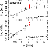
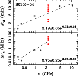
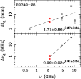
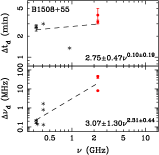
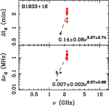
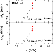
Figure 12: Frequency dependencies of decorrelation bandwidths and scintillation time-scales for eight pulsars. Asterisks represent previous measurements listed in Table 2, and dots are our new measurements as listed in Table 3. The dashed lines represent the best power-law fitting as given in the lower-right corner of each panel.

4.1 Frequency dependence of scintillation parameters

Observations with a wide frequency range are important to investigate the frequency dependencies of scintillation parameters and then the turbulent feature of the interstellar medium. For the widely accepted Kolmogorov turbulence, it was predicted that $\Delta t_{d}\propto\nu^{\alpha_{t}=6/5}$, $\Delta\nu_{d}\propto\nu^{\alpha_{\nu}=22/5}$, as shown by Equation 1. Combining previous measurements at various frequencies in Table 2 with our newly determined decorrelation bandwidths and scintillation time scales at 2250 MHz in Table 3, we can investigate the frequency dependence of scintillation parameters. Data are shown in Fig. 12, except for PSRs B2324+60 and B2351+61 because merely our measurements at S-band are available and there are no data at other frequencies. For seven pulsars our new data of decorrelation bandwidths are at the highest frequencies, and for PSR B0740-28 ours are at the lowest one. For four pulsars, PSRs B1508+55, B1933+16, B2154+40 and B2310+42, only few measurements are available and our measurements are crucial in determining the frequency dependencies of their scintillation parameters. For PSRs B0329+54, B0355+54, B0540+23 and B0740$-$28, the scintillation parameters roughly agree with the previous measurements by following a power-law. In general for these 8 pulsars, the power-indices for the decorrelation bandwidth vary greatly from 2.91 to 4.23, and only that of PSR B0540+23 is close to 4.4 for the Kolmogorov turbulence. Therefore, power-indices for the decorrelation bandwidth are generally smaller than the predictions by the Kolmogorov turbulence. The power-indices for the scintillation time scale vary greatly in the range from 0.71 to 0.87, also smaller than the predictions by the Kolmogorov turbulence, which has previously been noticed by Johnston et al. (1998); Bhat et al. (2004); Wang et al. (2005); Lewandowski et al. (2011). Moreover, by investigating the characteristic time of scattering, Geyer et al. (2017) also noticed that the frequency dependence is more complex than simple power law. Therefore the intervening medium between a pulsar and us can rarely be ideally turbulent with a Kolmogorov spectrum.

It should be noted, however, that the interstellar turbulence should be examined by using the scintillation parameters at different frequencies observed at the same epoch for the same medium, because pulsars move fast and the interstellar medium that they shine through is different at different epochs. Ideal observations should be done with a wide-band receiver to determine the instantaneous turbulence feature of the interstellar medium.

4.2 Scintillation velocity

The scintillation velocity $V_{\rm s}$ is effectively the combination of the transverse velocities of the pulsar, the intervening medium and the Earth, which can be derived from scintillation observations according to Equation 2. The dominant contribution in scintillation velocity is the transverse velocity of a pulsar, so that the pulsar velocities measured by other means are well-correlated with scintillation velocity (Lyne & Smith 1982; Cordes 1986; Gupta 1995; Bhat et al. 1999b).

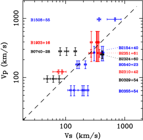
Figure 13: Comparison of proper motion velocities $V_{\rm p}$ (see Table 1) of pulsars with scintillation velocities $V_{\rm s}$ (see Table 3). The dashed line indicates the equality.

For ten pulsars that we observed (see Fig. 13), we estimated $V_{\rm s}$ from our observations by using Equation 2, as listed in Table 3, slightly different for different sessions for a given pulsar. We find that scintillation velocities are roughly consistent with proper motion velocities within two times the uncertainties except for PSRs B0355+54, B0740-28 and B2324+60.

It is understandable for the velocity estimated by Equation 2 for a thin screen model to slightly deviate from real velocities. Gupta (1995) attributed the differences for PSR B0355+54 to the enhanced scattering at low heights above the Galactic plane. As derived from its secondary spectrum analysis (see below and Table 4), the scattering screen of PSR B0355+54 locates closely to the pulsar, while the velocity estimation based on Equation 2 assumes that the screen lies at the midway between the pulsar and us, which therefore is a significantly over-estimate. So is that of PSR B2154+40. Moreover, the intervening medium rarely follows the Kolmogorov turbulence, as discussed above.

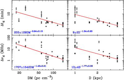
Figure 14: Scintillation parameters at 2250 MHz versus distance and dispersion measures for ten pulsars. The lines represent the best power-law fitting with the results given in the lower-left corner of each panel.

4.3 Scintillation parameters versus distance

For the Kolmogorov turbulence, scintillation parameters are related to pulsar distance theoretically by $\Delta t_{d}\propto D^{-3/5}$, $\Delta\nu_{d}\propto D^{-11/5}$, as shown by Equation 1. The distances are closely related to dispersion measures of these pulsars. By analyzing a series of measurements at 430 MHz, Cordes et al. (1985) found that $\Delta\nu_{d}\propto\rm DM^{-\gamma}$ with power index $\gamma=3-4$, much steeper than the theoretical prediction of $11/5$. This confirmed the previous analysis by multi-frequency observations scaled to 408 MHz (Rickett 1970, 1977), and it was attributed to variations of the level of turbulence $C_{n}^{2}$ over a wide range of length scales.

The pulsars we observed cover a wider range of DMs (see Table 1) than those in literature. As clearly seen from Figs. 1 to 11, pulsars with larger DMs tend to have smaller scintles in the dynamic spectra. Fig. 14 shows the change of scintillation parameters with pulsar DM and distance. Both $\Delta\nu_{d}$ and $\Delta t_{d}$ measured at S-band decrease with DM and distance by following a power-law, with indices of $-0.94\pm 0.15$ and $-1.34\pm 0.20$ for $\Delta t_{d}$ and $-1.43\pm 0.21$ and $-1.77\pm 0.33$ for $\Delta\nu_{d}$. The distance dependence for $\Delta\nu_{d}$ is roughly consistent with the prediction by the Kolmogorov turbulence with a large scatter of data, but the index for $\Delta t_{d}$ is steeper than that of the Kolmogorov turbulence. This contrasts to results at low frequencies (e.g. Rickett 1970, 1977; Cordes et al. 1985).

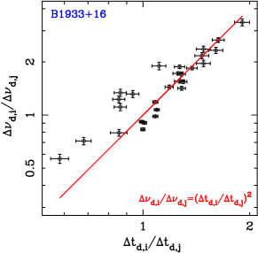
Figure 15: The ratio data of PSR B1933+16 for 28 paired epochs are consistent with the thin screen model which suggests that the ratio of decorrelation bandwidths of a paired epochs should have a quadratic relation with the ratio of scintillation time scales. A log-log plot is shown here with a linear fitting indicated by the solid line.

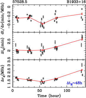
Figure 16: The scintillation parameters (open circles) calculated from every 1-hour block in 5 observational sessions of PSR B1933+16 since the epoch at 57528.5. They vary from those (dots) derived from data of an entire session listed in Table 2. The refractive scintillation is indicated by the long term variations of these parameters at different sessions.

4.4 Diffractive and refractive scintillation of PSR B1933+16

In the diffractive scintillation scheme, the scatter broadened image of a pulsar extends to an angular radius of $\theta_{d}$. In the thin screen model (e.g. Cordes 1986; Rickett 1990), it was predicted that $\Delta\nu_{d}=C_{1}c/(2\pi D\theta_{d}^{2})$ and $\Delta t_{d}=c/(2\pi\nu V_{\rm s}\theta_{d})$. For a given pulsar, although scintillation parameters vary among different observation sessions, both the ratio of $\Delta\nu_{d}$ and the radio of $\Delta t_{d}$ from a paired sessions should be related to $\theta_{d}^{2}$ or $\theta_{d}$, and therefore we get

$$\Delta\nu_{d,i}/\Delta\nu_{d,j}=(\Delta t_{d,i}/\Delta t_{d,j})^{2}.$$ (12)

By using the scintillation parameters ($\Delta\nu_{d}$, $\Delta t_{d}$) obtained for the 8 observational sessions of PSR B1933+16 as listed in Table 3, we verified the above scaling relations, as shown in Fig. 15. For any pair of observations, $i$ and $j$, we get $\Delta\nu_{d,i}/\Delta\nu_{d,j}$ and $\Delta t_{d,i}/\Delta t_{d,j}$, and they follow the relation very well. We therefore conclude that the thin screen model works well at S-band for the pulsar scintillation.

Refractive scintillation accounts for focusing of rays within the scattering disk with a scale $D\theta_{d}$. The time scale of refractive scintillation is related to diffractive scintillation parameters by (Stinebring & Condon 1990)

$$\Delta t_{R}\simeq(4/\pi)(\nu/\Delta\nu_{d})\Delta t_{d}.$$ (13)

The scintillation parameters of PSR B1933+16 in Table 3 give $\Delta t_{R}\sim 48$ hours, which is shorter than but comparable with our quasi continuous observations of 130 hours since the epoch of 57528.5. To investigate their variations in detail, we obtained the decorrelation bandwidth, scintillation time scale and the drift rate for every 1-hour block of data, as shown in Fig. 16. The variations at shorter time scales of hours might be caused by diffractive scintillation, and obvious long-term variations should come from the refraction from irregularities of interstellar medium. However, it is hard to get $\Delta t_{R}$ directly from the pulsar intensity fluctuations of our limited data.

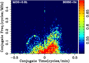
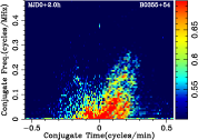
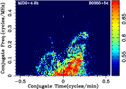
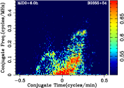
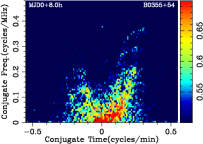
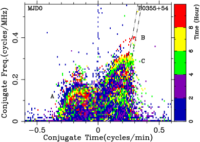
Figure 17: Upper five panels: Secondary spectra of PSR B0355+54 for five 2-hour blocks of data started at MJD0 = 57416.036 + 105 minutes, extracted from the 12 hour observation session of 57416.036 (see Fig. 2). The bottom panel: Evolving secondary spectra plotted only for the maximum power among the five 2-hour blocks of data for each pixel. Different color scales are used to mark which block of data for the maximum power. Three special inverted arclets are labeled by A, B and C, and the main parabola is indicated by the dashed lines.

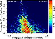
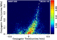
Figure 18: Secondary spectra of PSR B0540+23 (left) and PSR B2154+40 (right).

Figure 19: Variation of conjugate-time, $f_{t}$, of the vertexes of arclets A and C over a 12-hour session for PSR B0355+54. Their corresponding angular positions, $\theta_{x}$, can be found according to the scales in the right side of each panel.

4.5 Secondary Spectra of PSRs B0355+54, B0540+23 and B2154+40

Well defined parabolic arcs have been detected in the secondary spectra of dynamic spectra for some of our observational sessions of PSRs B0355+54, B0540+23 and B2154+40, as shown in Fig. 17 and Fig. 18. They are very asymmetric about the conjugate frequency axis. Previous detections of the arcs in the secondary spectra were made by Stinebring (2007) and Xu et al. (2018) for PSRs B0355+54 and by Safutdinov et al. (2017) for PSR B2154+40. For PSR B0540+23, this is the first time to report the detection of the arc, and its left branch is much more significantly shown. For PSRs B0355+54 and B2154+40, the right branches are much more significant. Refraction and the corresponding relatively large phase gradients of the interstellar medium are the main cause of the observed asymmetry. An-extreme-scattering like event happened along the sight line of PSR B0355+54 around MJD 57416, as indicated by the significant decrease in the scintillation parameters and the sharply peaked arcs of the secondary spectrum.

Table 4: The curvatures of parabolic arc, $\Omega$, of secondary spectra are used to estimate locations $d$ of scattering screens by assuming that pulsar velocity dominates and that any linear structure in the scattered image is aligned along the effective velocity vector.

PSRs	MJD	$\Omega$	$d$	$D_{\rm scr}$	$r_{v}$	$d_{\rm iss}$
		($s^{3}$)		(kpc)
B0355+54	57416.036	0.0216	0.081	0.92	0.256	0.062
B0540+23	57198.154	0.0648	0.556	0.69	0.982	0.491
B2154+40	58057.533	0.0252	0.398	1.75	0.868	0.430

The curvatures of the parabolic arcs, $\Omega$, can be estimated from the fittings to secondary spectra, which are closely related to the locations of the scattering screens $d$ (Hill et al. 2003), see the derived parameters listed in Table 4 for three pulsars. For PSR B0355+54, the curvature of the right part of the main parabola in the secondary spectrum as indicated by the dashed lines in Fig. 17 has been used to estimate $d=0.081$. Based on the known distances of pulsars in Table 1, the real distances of the screens $D_{\rm scr}$ are then determined. It should be noted that Equation 6 holds true only when the transverse velocities for the observer ${\@vec{V}}_{\rm obs}$ and the screen ${\@vec{V}}_{\rm scr}$ are negligible in the effective velocity of ${\@vec{V}}_{\rm eff}=(1-d){\@vec{V}}_{\rm p}+d{\@vec{V}}_{\rm obs}-{\@vec{V}}_{\rm scr}$ and when the angle between the orientation of the scattered image and ${\@vec{V}}_{\rm eff}$ is small. In the thin screen model, the location of the scattering screen can also be derived by using $r_{v}=V_{\rm p}/V_{\rm s}$ as introduced by Gupta (1995), and the location of a screen is (Stinebring et al. 2001) $d_{\rm iss}=r_{v}^{2}/(1+r_{v}^{2})$. For PSR B0355+54, $d_{\rm iss}=0.062$ that is consistent with $d$. We noticed that the screen we observed was closer to the pulsar PSR B2154+40, very different from that observed by Safutdinov et al. (2017). The screen we observed for PSR B0540+23 was somehow located halfway to the pulsar.

PSR B0355+54 also exhibits numerous isolated inverted parabolas in Fig. 17, and their vertices vaguely presented near the primary arc. The isolated arclets are probably caused by interference of the fine substructures in the scattered images of the pulsar (Cordes et al. 2006). These inverted arclets are also not distributed symmetrically, and are located at different positions in the secondary spectrum at different epochs. The arclet “A” in the left branch gradually shifts downwards along the main parabola, and the arclet “C” in the right branch moves to right upwards, and the arclet “B” is detected only once at the latest epoch in the top right part of the main parabola. This is only the second case to our knowledge that such an evolution behavior of inverted arclets has been reported, and the previous report was made for PSR B0834+06 by Hill et al. (2005) observed over 26 days at 321 MHz.

The evolution of the arclets is more clearly shown in the bottom panel of Fig. 17 by plotting the maximum of each pixels of 5 blocks with different color scales. In order to quantitatively describe their evolution, we determined the positions of the arclets from each block of data by following Hill et al. (2005). An inverted arclet model was first constructed, which has similar curvature as those in the secondary spectrum. The apex of the model was then fixed to a given position in the secondary spectrum, and the power was integrated along the arclet model. The two dimensional distribution of arclet power across apex positions was calculated by sliding the model across the secondary-spectrum plan. Through the plot, accurate positions for arclets A and C were determined, which evolved with time as shown in Fig. 19. Because the arclets are generally caused by separated deflecting interstellar medium structures at various angles $\theta$, the conjugate time $f_{t}$ (i.e. the abscissa of Fig. 17) can be related to the angular position $\theta$ by $f_{t}=-\theta_{x}V_{\rm eff}/(\lambda d)$, here, $\lambda$ is the observing wavelength, and $\theta_{x}$ is the angular position of the scattering structure along the effective velocity direction. By measuring the moving rate of the arclets across the main parabola, i.e., $\delta f_{t}/\delta t$, the angular velocity for the detected scattering structures can be estimated as

$$\delta\theta_{x}/\delta t=-(\lambda d/V_{\rm eff})\delta f_{t}/\delta t.$$ (14)

The linear fitting to data in Fig. 19 gives the arclet A moving across the conjugate time axis at a rate of 0.0027(9) per hour, and arclet B at a rate of 0.0034(13) per hour, again here the numbers in brackets are uncertainties for the last digit. Both the rates agree with each other and correspond to the angular velocities of $\delta\theta_{x}/\delta t\simeq$ 14(5) and 18(7) mas yr^-1. They are consistent with pulsar proper motions obtained by VLBI measurement of (9.2, 8.2) mas yr^-1 in the right ascension and declination (Chatterjee et al. 2004). The change of the angular position over the entire 12 hours of observations implies that the dense medium structure responsible for the scattering is much larger than 0.02 AU.

5 Conclusions

We have carried out long observation sessions to observe the scintillations of ten pulsars at S-band by using the Jiamusi 66-m telescope. The newly observed dynamic spectra were mostly at the highest frequencies for these pulsars, and some of them are the first dynamic spectra ever published. The decorrelation bandwidths and time scales of diffractive scintillation are derived from fitting to the main peak of autocorrelation functions of dynamic spectra. Well-defined parabolic arcs have been detected in the secondary spectra of some sessions of PSRs B0355+54, B0540+23 and B2154+40, which were used to determine the locations of the scattering screens. The evolution of inverted arclets in the secondary spectrum of PSR B0355+54 was observed, the angular velocity estimated from which was consistent with VLBI measurement.

Our measurements show that scintillation parameters vary from session to session. The frequency dependencies of both $\Delta t_{d}$ and $\Delta\nu_{d}$ imply that the turbulence feature of the interstellar medium deviates from the Kolmogorov turbulence. It is natural that the intervening medium cannot be so ideally turbulent. However, the thin screen model still holds well for PSR B1933+16. The scintillation velocities are only a rough indication of the pulsar velocities.

Data for dynamic spectra of all pulsars presented in this paper are available at http://zmtt.bao.ac.cn/psr-jms/.