Iteration-Complexity of the Subgradient Method on Riemannian Manifolds with Lower Bounded Curvature

Abstract

The subgradient method for convex optimization problems on complete Riemannian manifolds with lower bounded sectional curvature is analyzed in this paper. Iteration-complexity bounds of the subgradient method with exogenous step-size and Polyak’s step-size are stablished, completing and improving recent results on the subject.
Keywords: Subgradient method, Riemannian manifold, complexity, convex programming, lower bounded curvature.

1 Introduction

In this paper we consider the subgradient method to solve the optimization problem defined by:

$$\min\{f(p)~{}:~{}p\in\mathcal{M}\},$$ (1)

where the constraint set $\mathcal{M}$ is endowed with a structure of a complete Riemannian manifold with lower bounded curvature and $f:\mathcal{M}\to\overline{\mathbb{R}}$ is a convex function, where $\overline{\mathbb{R}}=\mathbb{R}\cup\{+\infty\}$ denotes the extended real set numbers.

It is well known that non-convex problems can be transformed into convex by introducing a suitable metric. As a consequence, this technique can be exploited in order to find global minimizers [4, 3, 7, 23] and to reduce the iteration-complexity of finding such solutions [2, 31]. Furthermore, many optimization problems are naturally posed on Riemannian manifolds which have a specific underlying geometric and algebraic structure that can be exploited to greatly reduce the cost of obtaining solutions. For instance, in order to take advantage of the Riemannian geometric structure, it is preferable to treat certain constrained optimization problems as problems for finding singularities of gradient vector fields on Riemannian manifolds rather than using Lagrange multipliers or projection methods; see [19, 25, 26]. Accordingly, constrained optimization problems are viewed as unconstrained ones from a Riemannian geometry point of view. Besides, Riemannian geometry also opens up new research directions that aid in developing competitive algorithms; see [9, 21, 25]. For this purpose, extensions of concepts and techniques of optimization from Euclidean space to Riemannian context have been quite frequent in recent years. Papers dealing with this subject include, but are not limited to [11, 17, 18, 27, 29, 20].

The subgradient method is a very simple algorithm for solving convex optimization problems and, besides it is the departure point for many other more sophisticated and efficient algorithms, including $\epsilon$-subgradient methods, bundle methods and cutting-plane algorithm; see [6] for a comprehensive study on this subject. The subgradient method was originally developed by Shor and others in the 1960s and 1970s and since of then, it and its variants have been applied to a far wider variety of problems in optimization theory; see[22, 13]. In order to deal with non-smooth convex optimization problems on complete Riemanian manifolds with non-negative sectional curvature, [12] extended and analyzed the subgradient method which, as in the Euclidean context, is quite simple and possess nice convergence properties. After this pioneering work, the subgradient method in the Riemannian setting has been studied in different contexts; see, for instance, [4, 27, 29, 14, 1]. In [4] the subgradient method was introduced to solve convex feasibility problems on complete Riemannian manifolds with non-negative sectional curvatures, and recently in [27, 29] this method has been analyzed in manifolds with lower bounded sectional curvatures and significant improvements were introduced. More recently, an asymptotic analysis of the subgradient method with exogenous step-size and dynamic step-size for convex optimization was considered in the context of manifolds with lower bounded sectional curvatures, see [28].

In this paper we establish an iteration-complexity bound of the subgradient method with exogenous step-size and Polyak’s step-size, for convex optimization problems on complete Riemannian manifolds with lower bounded sectional curvatures. Our results increase the range of applicability of the method compared to the respective results obtained in [2, 31, 32]. Moreover, in the asymptotic analysis with exogenous step-size, we do not assume that the solution set is nonempty, completing the result of [28, Theorem 3.1]. It should be noted that our analysis use a recently inequality stablished in [27, 29].

This paper is organized as follows. Section 2 presents some definitions and preliminary results related to the Riemannian geometry that are important to our study. In Section 3, we obtain iteration-complexity bounds and other convergence results of the subgradient method with exogenous step-size and Polyak’s step-size. In the Section 4 we use the convex feasibility problem for numerically illustrate the results on complexity-iteration bounds of Section 3. The last section contains a conclusion.

2 Notations and basic concepts

In this section, we introduce some fundamental properties and notations about Riemannian geometry. These basics facts can be found in any introductory book on Riemannian geometry; see for example, [8, 24]. We also recall the definitions of convexity of function and Lipschitz continuity in the Riemannian setting and present some basic properties related to these concepts that will be essential for the analyses of the subgradient method in the next section.

In this paper $\mathcal{M}$ is endowed with a structure of a complete Riemannian manifold with lower bounded curvature. Throughout the paper we also assume that the sectional curvature of $\mathcal{M}$ is bounded below by $\kappa<0$. We denote by $T_{p}\mathcal{M}$ the tangent space of a Riemannian manifold $\mathcal{M}$ at $p$. The corresponding norm associated to the Riemannian metric $\langle\cdot,\cdot\rangle$ is denoted by $\|\cdot\|$. We use $\ell(\alpha)$ to denote the length of a piecewise smooth curve $\alpha:[a,b]\rightarrow\mathcal{M}$. The Riemannian distance between $p$ and $q$ in a finite dimensional Riemannian manifold $\mathcal{M}$ is denoted by $d(p,q)$, which induces the original topology on $\mathcal{M}$, namely, $(\mathcal{M},d)$ is a complete metric space where bounded and closed subsets are compact. Let $\nabla$ be the Levi-Civita connection associated to $(\mathcal{M},\langle\cdot~{},~{}\cdot\rangle)$. A vector field $V$ along $\gamma$ is said to be parallel iff $\nabla_{\gamma^{\prime}}V=0$. If $\gamma^{\prime}$ itself is parallel we say that $\gamma$ is a geodesic. Since the geodesic equation $\nabla_{\ \gamma^{\prime}}\gamma^{\prime}=0$ is a second order nonlinear ordinary differential equation, then the geodesic $\gamma=\gamma_{v}(\cdot,p)$ is determined by its position $p$ and velocity $v$ at $p$. It is easy to check that $\|\gamma^{\prime}\|$ is constant. The restriction of a geodesic to a closed bounded interval is called a geodesic segment. A geodesic segment joining $p$ to $q$ in $\mathcal{M}$ is said to be minimal if its length is equal to $d(p,q)$. Hopf-Rinow’s theorem asserts that any pair of points in a complete Riemannian manifold $\mathcal{M}$ can be joined by a (not necessarily unique) minimal geodesic segment. Due to the completeness of the Riemannian manifold $\mathcal{M}$, the exponential map $\exp_{p}:T_{p}\mathcal{M}\to\mathcal{M}$ can be given by $\exp_{p}v\,=\,\gamma_{v}(1,p)$, for each $p\in\mathcal{M}$. We proceed by recalling some concepts and basic properties about convexity in the Riemannin context. For more details see, for example, [26, 23]. For any two points $p,q\in\mathcal{M}$, $\Gamma_{pq}$ denotes the set of all geodesic segments $\gamma:[0,1]\rightarrow\mathcal{M}$ with $\gamma(0)=p$ and $\gamma(1)=q$. The closed metric ball in $\mathcal{M}$ centered at the point $p\in\mathcal{M}$ with radius $r>0$ is denoted by $B[p,r]$. Let $\Omega$ be a subset of $\mathcal{M}$. We use $\emph{int}~{}\Omega$ to denote the interior of $\Omega$. A function $f:\mathcal{M}\rightarrow\overline{\mathbb{R}}$ is said to be proper if its domain $\emph{dom}f=\{p\in\mathcal{M}:f(p)\neq+\infty\}$ is nonempty, where $\overline{\mathbb{R}}=\mathbb{R}\cup\{+\infty\}$ denotes the extended real set numbers. We use $\Gamma^{f}_{pq}$ to denote the set of all $\gamma\in\Gamma_{pq}$ such that $\gamma\subseteq\emph{dom}f$. A nonempty subset $\Omega\subset\mathcal{M}$ is said to be weakly convex if, for any $p,q\in\Omega$, there is a minimal geodesic segment joining $p$ to $q$ and it is in $\Omega$. A proper function $f:\mathcal{M}\to\overline{\mathbb{R}}$ is said to be convex on $\mathcal{M}$ if $\emph{dom}f$ is weakly convex and for any $p,q\in\emph{dom}f$ and $\gamma\in\Gamma^{f}_{pq}$ the composition $f\circ\gamma:[0,1]\to\overline{\mathbb{R}}$ is a convex function on $[0,1]$ i.e.,

$$f\circ\gamma(t)\leq(1-t)f(p)+tf(q),\qquad\forall~{}t\in[0,1],$$

see [27]. The subdifferential of a convex function $f:\mathcal{M}\rightarrow\overline{\mathbb{R}}$ at $p\in\emph{dom}f$ is defined by

$$\partial f(p):=\left\{s\in T_{p}\mathcal{M}:f(q)\geq f(p)+\left\langle s,\gamma^{\prime}(0)\right\rangle,\quad\forall~{}y\in\emph{dom}f,~{}\gamma\in\Gamma^{f}_{pq}\right\}.$$ (2)

We remark that the subdiffential set $\partial f(p)$ is nonempty in all at $p\in\emph{int}\,\emph{dom}f$; see [27, Proposition 2.5]. In this paper all functions $f:\mathcal{M}\to\overline{\mathbb{R}}$ is assumed to be convex and lower semicontinuous on $\mathcal{M}$. The following result is also proved in [27, Proposition 2.5].

Proposition 1.

Let $\{p_{k}\}\subset\mathcal{M}$ a bounded sequence. If the sequence $\{s_{k}\}$ is such that $s_{k}\in\partial f(p_{k})$, for each $k\in\mathbb{N}$, then $\{s_{k}\}$ is also bounded.

The following lemma plays an important role in the next sections. Its proof will be omitted here, but it can be obtained, with some minor technical adjustments, by using the Toponogov’s theorem [24, p.161, Theorem 4.2] and following the ideas of [27, Lemma 3.2]; see also [29].

Lemma 1.

Let $p\in\emph{int}\,\emph{dom}f$, $0\neq s\in\partial f(p)$, and let $\gamma:[0,+\infty)\rightarrow\mathcal{M}$ be the geodesic defined by ${\gamma}(t)=\mbox{exp}_{p}\left(-ts/\left\|s\right\|\right).$ Then, for any $t\in[0,\infty)$ and $q\in\emph{dom}f$ there holds

$$\cosh(\sqrt{|\kappa|}d(\gamma(t),q))\leq\cosh(\sqrt{|\kappa|}d(p,q))+\\ \sqrt{|\kappa|}\cosh(\sqrt{|\kappa|}d(p,q))\sinh(t\sqrt{|\kappa|})\left[\frac{t}{2}-\frac{\tanh(\sqrt{|\kappa|}d(p,q))}{\sqrt{|\kappa|}d(p,q)}\frac{f(p)-f(q)}{\left\|s\right\|}\right]$$

and, consequently, the following inequality holds

$$d^{2}({\gamma}(t),q)\leq d^{2}(p,q)+\frac{\sinh\left(\sqrt{|\kappa|}t\right)}{\sqrt{|\kappa|}}\left[\frac{\sqrt{|\kappa|}d(p,q)}{\tanh\left(\sqrt{|\kappa|}d(p,q)\right)}t-\frac{2}{\left\|s\right\|}\left(f(p)-f(q)\right)\right].$$

The next concept will be useful in the analysis of the sequence generated by the subgradient method.

Definition 1.

A sequence $\{y_{k}\}$ in the complete metric space $(\mathcal{M},d)$ is quasi-Fejér convergent to a set $W\subset\mathcal{M}$ if, for every $w\in W$, there exists a sequence $\{\epsilon_{k}\}\subset\mathbb{R}$ such that $\epsilon_{k}\geq 0$, $\sum_{k=1}^{\infty}\epsilon_{k}<+\infty$, and

$$d^{2}(y_{k+1},w)\leq d^{2}(y_{k},w)+\epsilon_{k},\qquad\forall~{}k.$$

The main property of the quasi-Fejér convergent sequence is stated in the next result, and its proof is similar to the one proved in [5] by replacing the Euclidean by the Riemannian distance.

Theorem 1.

Let $\{y_{k}\}$ be a sequence in the complete metric space $(\mathcal{M},d)$. If $\{y_{k}\}$ is quasi-Fejér convergent to a nomempty set $W\subset\mathcal{M}$, then $\{y_{k}\}$ is bounded. If furthermore, a cluster point $y$ of $\{y_{k}\}$ belongs to $W$, then $\lim_{k\rightarrow\infty}y_{k}=y$.

We end this section by recalling the concept of Lipschitz continuity of a function. A proper function $f:\mathcal{M}\to\overline{\mathbb{R}}$ is said to be Lipschitz continuous with constant $\tau\geq 0$ in $\Omega\subset\mathcal{M}$ if $\left|f(p)-f(q)\right|\leq\tau\,d(p,q)$, for any $p,q\in\Omega$.

3 Iteration-Complexity of the Subgradient Method

In this section, we state the Riemannian subgradient method to solve (1) and the strategies for choosing the step-size that will be used in our analysis. Let $f:\mathcal{M}\to\overline{\mathbb{R}}$ be convex function, $\Omega^{*}$ be the solution set of the problem (1) and $f^{*}\coloneqq\inf_{x\in\mathcal{M}}f(x)$ be the optimum value of $f$. In our analysis we do not assume that $\Omega^{*}$ is nonempty, except when explicitly stated. The statement of Riemannian subgradient algorithm to solve the problem (1) is as follows.

Step 0.

Let $p_{0}\in\emph{int}\,\emph{dom}f$. Set $k=0$.

Step 1.

If $s_{k}=0$, then stop; otherwise, choose a step-size $t_{k}>0$, $s_{k}\in\partial f(p_{k})$ and compute

$$p_{k+1}:=\exp_{p_{k}}\left(-t_{k}\frac{s_{k}}{\|s_{k}\|}\right);$$ (3)

Step 2.

Set $k\leftarrow k+1$ and proceed to Step 1.

Algorithm 1 Subgradient algorithm in a Riemanian manifold $\mathcal{M}$

In the following we present two different strategies for choosing the step-size $t_{k}>0$ in Algorithm 1.

Strategy 1 (Exogenous step-size).

$$t_{k}>0,\qquad\qquad\sum_{k=0}^{\infty}t_{k}=+\infty,\qquad\qquad\sigma:=\sum_{k=0}^{\infty}t_{k}^{2}<+\infty.$$ (4)

The step-size in Strategy 1 have been used in several paper for analyzing subgradient method; see, for example, [12, 6, 28].

Strategy 2 (Polyak’s step-size).

Assume that $p_{0}\in\emph{int}\,\emph{dom}f$, $\Omega^{*}\neq\varnothing$ an set

$$t_{k}=\alpha\frac{f(p_{k})-f^{*}}{\left\|s_{k}\right\|},\qquad 0<\alpha<2\frac{\tanh\left(\sqrt{|\kappa|}d_{0}\right)}{\sqrt{|\kappa|}d_{0}},\qquad d_{0}:=d(p_{0},\Omega^{*}),$$ (5)

where $d(p_{0},\Omega^{*}):=\inf\{d(p_{0},q);~{}q\in\Omega^{*}\}>0$.

This step-size in Strategy 2 was introduced in [22] and has been used in [2, 4, 27].

Remark 1.

Since the function $(0,+\infty)\mapsto\tanh(t)/t$ is decreasing, then given an estimate $\hat{d}>d_{0}$ we can chose $0<\alpha<2\tanh(\sqrt{|\kappa|}\hat{d})/(\sqrt{|\kappa|}\hat{d}))$ in Strategy 2. For Riemannian manifold with non-negative curvature, the second inequality in (5) holds for all $\kappa<0$. Due to $\lim_{t\to 0}\tanh(t)/t=1$, letting $\kappa$ goes to $0$, we can chose $0<\alpha<2$.

From now on we assume that the sequence $\{p_{k}\}$ generated by Algorithm 1 with the two above strategies for choosing the step-size is well defined and is infinite.

Remark 2.

Note that if $\emph{dom}f=\mathcal{M}$ then $\partial f(p)\neq\varnothing$, for all $p\in\mathcal{M}$ and, consequently, the sequence $\{p_{k}\}$ is well defined. In [28, Theorem 3.1] an asymptotic convergence analysis was established, under the assumption that suitable sets are contained in $\emph{int}\,\emph{dom}f$ and that the set $\Omega^{*}$ is nonempty. The author proves that the sequence generated by the Algorithm 1 is well defined and converges to an element of $\Omega^{*}$. It is worth to pointed out that our asymptotic convergence analysis of Algorithm 1, with Strategy 1 for choosing the step-size, we do not assume that $\Omega^{*}$ is nonempty. In this sense, our results improve the ones of [28, Theorem 3.1].

3.1 Subgradient Method with Exogenous Stepsize

In this section we assume that the sequence $\{p_{k}\}$ is generated by Algorithm 1 with Strategy 1 for choosing the step-size. To proceed with the analysis of the Algorithm 1 we need some preliminaries. Firstly we define

$$\Omega:=\left\{q\in\mathcal{M}:~{}f(q)\leq\inf_{k}f(p_{k})\right\}.$$ (6)

Note that $\Omega\subset\emph{dom}f$. It is worth mentioning that, in principle, the set $\Omega$ can be empty. Our first task is to prove that the sequence $\{p_{k}\}$ is bounded.

Lemma 2.

If $\Omega\neq\varnothing$ then, for each $q\in\Omega$ there holds

$$d(p_{k+1},q)\leq\frac{1}{\sqrt{|\kappa|}}\cosh^{-1}\left(\cosh\left(\sqrt{|\kappa|}d(p_{0},q)\right)e^{\frac{1}{2}\sqrt{\sigma|\kappa|}\sinh\left(\sqrt{\sigma|\kappa|}\right)}\right),$$ (7)

for all $k=0,1,\ldots.$.

Proof.

Applying first inequality of Lemma 1 with $t=t_{k}$, $p=p_{k}$ and $p_{k+1}=\gamma(t_{k})$ and taking into account that $q\in\Omega$ we conclude that

$$\cosh\left(\sqrt{|\kappa|}d(p_{k+1},q)\right)\leq\cosh\left(\sqrt{|\kappa|}d(p_{k},q)\right)\left[1+|\kappa|t_{k}^{2}\frac{\sinh\left(\sqrt{|\kappa|}t_{k}\right)}{2\sqrt{|\kappa|}t_{k}}\right],\qquad k=0,1,\ldots.$$

Using definition of $\sigma$ in (4) we have $t_{k}\leq\sqrt{\sigma}$, for all $k=0,1,\ldots$. Since the map $(0,+\infty)\ni t\mapsto\sinh(t)/t$ is increasing, it follows from the last inequality that

$$\cosh\left(\sqrt{|\kappa|}d(p_{k+1},q)\right)\leq\cosh\left(\sqrt{|\kappa|}d(p_{k},q)\right)\left[1+at_{k}^{2}\right],\qquad k=0,1,\ldots,$$

where $a:=\sqrt{|\kappa|}(\sinh(\sqrt{\sigma|\kappa|}))/(2\sqrt{\sigma})$. Note that the last inequality implies that

$$\cosh\left(\sqrt{|\kappa|}d(p_{k+1},q)\right)\leq\cosh\left(\sqrt{|\kappa|}d(p_{k},q)\right)e^{at_{k}^{2}},\qquad k=0,1,\ldots.$$

Therefore, we have $\cosh(\sqrt{|\kappa|}d(p_{k+1},q))\leq\cosh(\sqrt{|\kappa|}d(p_{0},q))e^{a\sigma}$, which is equivalent to (7) and the proof is concluded. ∎

In the next result we apply Lemmas 1 and 2 to derive an inequality that plays an important role in our analysis, which is a generalization of the one obtained in [12, Lemma 4.1]. In the linear setting, this inequality is of fundamental importance to analyze the subgradient method; see, for example, [6]. It is worth noting that it was obtained in [30] for an specific function, namely, the mean function. For stating the next result, for each $q\in\Omega$, we define

$$C_{q,\kappa}:=\frac{\sinh\left(\sqrt{\sigma\left|\kappa\right|}\right)}{\sqrt{\sigma\left|\kappa\right|}}\left[1+\cosh^{-1}\left(\cosh(\sqrt{\left|\kappa\right|}d(p_{0},q))e^{\frac{1}{2}\sqrt{\sigma\left|\kappa\right|}\sinh\left(\sqrt{\sigma\left|\kappa\right|}\right)}\right)\right].$$ (8)

It is important to note that $C_{q,\kappa}$ is well defined only under the assumption $\Omega\neq\varnothing$.

Lemma 3.

If $\Omega\neq\varnothing$ then, for each $q\in\Omega$ there holds

$$d^{2}(p_{k+1},q)\leq d^{2}(p_{k},q)+C_{q,\kappa}t_{k}^{2}+2\,\frac{t_{k}}{\left\|s_{k}\right\|}[f(q)-f(p_{k})],\qquad s_{k}\in\partial f(p_{k}),\qquad k=0,1,\ldots.$$

Proof.

Applying first inequality of Lemma 1 with $t=t_{k}$, $p=p_{k}$ and $p_{k+1}=\gamma(t_{k})$, and taking into account that $q\in\Omega$, we conclude that

$$d^{2}(p_{k+1},q)\leq d^{2}(p_{k},q)+\frac{\sinh\left(\sqrt{|\kappa|}t_{k}\right)}{\sqrt{|\kappa|}t_{k}}\left[\frac{\sqrt{|\kappa|}d(p_{k},q)}{\tanh\left(\sqrt{|\kappa|}d(p_{k},q)\right)}t_{k}^{2}+\frac{2t_{k}}{\|s_{k}\|}\left[f(q)-f(p_{k})\right]\right],$$

for all $k=0,1,\ldots$. On the other hand, $t/\tanh(t)\leq 1+t$, for all $t\geq 0$ and the map $(0,+\infty)\ni t\mapsto\sinh(t)/t$ is increasing and bounded below by $1$. Thus, taking into account that $t_{k}\leq\sqrt{\sigma}$ and $f(q)-f(p_{k})\leq 0$, for all $k=0,1,\ldots$, we conclude that

$$d^{2}(p_{k+1},q)\leq d^{2}(p_{k},q)+\frac{\sinh\left(\sqrt{\sigma|\kappa|}\right)}{\sqrt{\sigma|\kappa|}}\left[1+\sqrt{|\kappa|}d(p_{k},q)\right]t^{2}_{k}+\frac{2t_{k}}{\|s_{k}\|}\left[f(q)-f(p_{k})\right],$$

for all $k=0,1,\ldots$. Therefore, combining Lemma 2 with (8) the desired inequality follows and the proof is concluded. ∎

Remark 3.

For Riemannian manifold with non-negative curvature, the inequality in Lemma 3 holds for all $\kappa<0$. Since $\lim_{\kappa\to 0}C_{q,\kappa}=1$, the inequality of the Lemma 3 merges into the inequality [12, Lemma 4.1].

y Now we ready to prove the main result of this section.

Theorem 2.

Assume that $\Omega^{*}\neq\varnothing$ and $f:\mathcal{M}\to\overline{\mathbb{R}}$ is Lipschitz continuous with constant $\tau\geq 0$. Then, for all $p_{*}\in\Omega^{*}$ and every $N\in\mathbb{N}$, the following inequality holds

$$\min\left\{f(p_{k})-f^{*}~{}:~{}k=0,1,\ldots,N\right\}\leq\tau\frac{d^{2}(p_{0},p_{*})+C_{p_{*},\kappa}\sum_{k=0}^{N}t_{k}^{2}}{2\sum_{k=0}^{N}t_{k}}.$$ (9)

Proof.

Let $p_{*}\in\Omega^{*}$. Since $\Omega^{*}\subset\Omega$, applying Lemma 3 with $q=p_{*}$, we obtain

$$d^{2}(p_{k+1},p_{*})\leqslant d^{2}(p_{k},p_{*})+C_{p_{*},\kappa}t_{k}^{2}+2\frac{t_{k}}{\|s_{k}\|}[f^{*}-f(p_{k})],\qquad s_{k}\in\partial f(p_{k}),$$

for all $k=0,1,\ldots$. Hence, performing the sum of the above inequality for $k=0,1,\ldots,N$, after some algebraic manipulations, we have

$$2\sum_{k=0}^{N}\frac{t_{k}}{\|s_{k}\|}[f(p_{k})-f^{*}]\leq d^{2}(p_{0},p_{*})-d^{2}(p_{N+1},p_{*})+C_{p_{*},\kappa}\sum_{k=0}^{N}t_{k}^{2}.$$

Since $f$ is Lipschitz continuous with constant $\tau\geq 0$, we have $\|s_{k}\|\leq\tau$, for all $k=0,1,\ldots$. Therefore,

$$\frac{2}{\tau}\min\left\{f(p_{k})-f^{*}:~{}k=0,1,\ldots,N\right\}\sum_{k=0}^{N}t_{k}\leq d^{2}(p_{0},p_{*})+C_{p_{*},\kappa}\sum_{k=0}^{N}t_{k}^{2},$$

which is equivalent to the desired inequality. ∎

Remark 4.

Note that, for Riemannian manifold with non-negative curvature the inequality in (9) holds for all $\kappa<0$. Since $\lim_{\kappa\to 0}C_{q,\kappa}=1$, Theorem 2 is reduced to [2, Theorem 3.3].

We remark that in the first part of the next theorem we do not assume that $\Omega^{*}\neq\varnothing$. Additionally, It is worth to point out that the second part was first obtained in [28]. Since it is an immediate consequence of the first part and Lemma 3, we decide to include its proof here.

Theorem 3.

The following equality holds

$$\liminf_{k}f(p_{k})=f^{*}.$$ (10)

In addition, if $\Omega^{*}\neq\varnothing$ then the sequence $\{p_{k}\}$ converges to a point $p_{*}\in\Omega^{*}$.

Proof.

Assume by contradiction that $\liminf_{k}f(p_{k})>f^{*}.$ In this case, we have $\Omega\neq\varnothing$. Thus, from Lemma 2, we conclude that $\{p_{k}\}$ is bounded and, consequently, by using Proposition 1, the sequence $\{s_{k}\}$ is also bounded. Let $C_{1}>0$ such that $\left\|s_{k}\right\|<C_{1}$, for $k=0,1,\ldots$. On the other hand, letting $q\in\Omega$, there exist $C_{2}>0$ and $k_{0}\in\mathbb{N}$ such that $f(q)<f(p_{k})-C_{2},$ for all $k\geq k_{0}$. Hence, using Lemma 3 and considering that $\left\|s_{k}\right\|<C_{1}$, for $k=0,1,\ldots$, we have

$$d^{2}(p_{k+1},q)\leq d^{2}(p_{k},q)+C_{q,\kappa}t^{2}_{k}-2\frac{C_{2}}{C_{1}}t_{k},\qquad k=k_{0},k_{0}+1,\dots.$$

Consider $\ell\in\mathbb{N}$. Thus, from the last inequality, after some calculations, we conclude that

$$\frac{2\,C_{2}}{C_{1}}\sum_{j=k_{0}}^{\ell+k_{0}}t_{j}\leq d^{2}(p_{k_{0}},q)-d^{2}(p_{k_{0}+\ell},q)+C_{q,\kappa}\sum_{j=k_{0}}^{\ell+k_{0}}t^{2}_{j}\leq d^{2}(p_{k_{0}},q)+C_{q,\kappa}\sum_{j=k_{0}}^{\ell+k_{0}}t^{2}_{j}.$$

Since the last inequality holds for all $\ell\in\mathbb{N}$, then using the inequality in (4) we have a contraction. Therefore, (10) holds.

For proving the last statement, let us assume that $\Omega^{*}\neq\varnothing$. In this case, we have $\Omega\neq\varnothing$ and, from Lemma 2, the sequence $\{p_{k}\}$ is bounded. Moreover, Lemma 3 implies, in particular, that $\{p_{k}\}$ is quasi-Féjer convergent to $\Omega$. The equality (10) implies that $\{f(p_{k})\}$ possesses a decreasing monotonous subsequence $\{f(p_{k_{j}})\}$ such that $\lim_{j\rightarrow\infty}f(p_{k_{j}})=f^{*}.$ We can assume that $\{f(p_{k})\}$ is decreasing, monotonous and converges to $f^{*}$. Being bounded, the sequence $\{p_{k}\}$ possesses a convergent subsequence $\{p_{k_{\ell}}\}$. Let us say that $\lim_{\ell\rightarrow\infty}p_{k_{\ell}}=p_{*},$ which by the continuity of $f$ implies $f(p_{*})=\lim_{\ell\rightarrow\infty}f(p_{k_{\ell}})=f^{*},$ and then $p_{*}\in\Omega$. Hence, $\{p_{k}\}$ has an cluster point $p_{*}\in\Omega$, and due to $\{p_{k}\}$ be quasi-Féjer convergent to $\Omega$, it follows from Theorem 1 that the sequence $\{p_{k}\}$ converges to $p_{*}$. ∎

3.2 Subgradient Method with Polyak Stepsize

In this section, we assume that $\Omega^{*}\neq\varnothing$ and $\{p_{k}\}$ is generated by Algorithm 1 with Strategy 2 for choosing the step-size. Let us define

$$C_{\kappa,d_{0}}:=\frac{2}{\alpha}-\frac{\sqrt{|\kappa|}d_{0}}{\tanh\left(\sqrt{|\kappa|}d_{0}\right)}>0,$$ (11)

where $\alpha$ and $d_{0}$ are defined in (5).

Remark 5.

Since $\lim_{t\to 0}\tanh(t)/t=1$, we conclude that for Riemannian manifolds with nonnegative curvature, namely, for $\kappa=0$, (11) become $C_{\kappa,d_{0}}\equiv 2/\alpha-1>0$.

In the next result, we apply Lemma 1 to obtain an inequality that plays an important role in our analysis. Before state this result, we set

$${\bar{q}}\in\Omega^{*}\quad\mbox{such that}\quad d_{0}=d(p_{0},{\bar{q}}).$$ (12)

Lemma 4.

Let ${\bar{q}}\in\Omega^{*}$ satisfying (12). Then the following inequality holds

$$d^{2}(p_{k+1},{\bar{q}})\leq d^{2}(p_{k},{\bar{q}})-C_{\kappa,d_{0}}\alpha^{2}\frac{\left[f(p_{k})-f^{*}\right]^{2}}{\left\|s_{k}\right\|^{2}},\qquad k=0,1,\ldots.$$

Proof.

First we are going to prove that $d(p_{k},{\bar{q}})\leq d_{0}$, for all $k=0,1,\ldots$. The proof will be made by induction. For $k=0$ is immediate. Assume that $d(p_{k},{\bar{q}})\leq d_{0}$. Using the second inequality of Lemma 1 with $q={\bar{q}}$, $t=t_{k}$, $p=p_{k}$, $s=s_{k}$, $p_{k+1}=\gamma(t_{k})$ and considering that $f^{*}=f({\bar{q}})$, we obtain

$$d^{2}(p_{k+1},{\bar{q}})\leq d^{2}(p_{k},{\bar{q}})+\frac{\sinh\left(\sqrt{|\kappa|}t_{k}\right)}{\sqrt{|\kappa|}t_{k}}\left[\frac{\sqrt{|\kappa|}d(p_{k},{\bar{q}})}{\tanh\left(\sqrt{|\kappa|}d(p_{k},{\bar{q}})\right)}t_{k}^{2}+\frac{2t_{k}}{\|s_{k}\|}\left[f^{*}-f(p_{k})\right]\right].$$

Since the map $(0,+\infty)\ni t\mapsto t/\tanh(t)$ is increasing, using the assumption $d(p_{k},{\bar{q}})\leq d_{0}$ and definition of $t_{k}$ in (5), the last inequality becomes

$$d^{2}(p_{k+1},{\bar{q}})\leq d^{2}(p_{k},{\bar{q}})+\frac{\sinh\left(\sqrt{|\kappa|}t_{k}\right)}{\sqrt{|\kappa|}t_{k}}\left[\,\frac{\sqrt{|\kappa|}d_{0}}{\tanh\left(\sqrt{|\kappa|}d_{0}\right)}-\frac{2}{\alpha}\right]\alpha^{2}\frac{\left[f(p_{k})-f^{*}\right]^{2}}{\left\|s_{k}\right\|^{2}}.$$ (13)

Thus, the inequalities in (5) imply that $d(p_{k+1},{\bar{q}})\leq d(p_{k},{\bar{q}})\leq d_{0}$ and the induction is concluded. Hence, $d(p_{k},{\bar{q}})\leq d_{0}$, for all $k=0,1,\ldots$. Therefore, we can also prove that (13) hods, for all $k=0,1,\ldots$. Taking into account that $\sinh(\sqrt{|\kappa|}t_{k})/(\sqrt{|\kappa|}t_{k})\geq 1$, the combination of second inequality in (5), (11) and (13) yield the desired inequality. ∎

Remark 6.

Since $\lim_{t\to 0}\tanh(t)/t=1$ and $\lim_{t\to 0}\sinh(t)/t=1$, then by using similar idea considered in the proof of Lemma 4, we can show that, for Riemannian manifolds with nonnegative curvature, holds $d^{2}(p_{k+1},q)\leq d^{2}(p_{k},q)-(2/\alpha-1)t^{2}_{k}$, for all $k=0,1,\ldots$ and all $q\in\Omega^{*}$.

The next result presents an iteration-complexity bound for the subgradient method with the Polyak’s step-size rule.

Theorem 4.

Assume that $f:\mathcal{M}\to\overline{\mathbb{R}}$ is Lipschitz continuous with constant $\tau\geq 0$. Let ${\bar{q}}\in\Omega^{*}$ satisfying (12). Then, for every $N\in\mathbb{N}$, there holds

$$\sum_{k=0}^{N}[f(p_{k})-f^{*}]^{2}\leq\frac{\tau^{2}d^{2}(p_{0},{\bar{q}})}{{C_{\kappa,d_{0}}}}.$$ (14)

As a consequence,

$$\min\left\{f(p_{k})-f^{*}~{}:~{}k=0,1,\ldots,N\right\}\leq[\tau d(p_{0},{\bar{q}})]/\sqrt{{C_{\kappa,d_{0}}}(N+1)}.$$ (15)

Proof.

Since $f$ is Lipschitz continuous with constant $\tau\geq 0$, we have $\|s_{k}\|\leq\tau$, for all $k=0,1,\ldots$. Thus, it follows from Lemma 4 that

$$[f(p_{k})-f^{*}]^{2}\leq\frac{\tau^{2}}{C_{\kappa,d_{0}}\alpha^{2}}[d^{2}(p_{k},{\bar{q}})-d^{2}(p_{k+1},{\bar{q}})],\qquad k=0,1,\ldots.$$

Performing the sum of the above inequality for $k=0,1,\ldots,N$, we obtain (14). The second statement of the theorem is an immediate consequence of the first one. ∎

Remark 7.

It is worth noting that if $\kappa=0$ we have $C_{q,\kappa}=1$ and then Theorem 4 merges into the inequality [2, Theorem 3.4].

Theorem 5.

The following equality holds $\lim_{k\rightarrow\infty}f(p_{k})=f^{*}$. Consequently, all cluster point of $\{p_{k}\}$ is a solution of (1).

Proof.

Letting $N$ goes to $+\infty$ in (14), we conclude that $\lim_{k\rightarrow\infty}f(p_{k})=f^{*}$. It follows from Lemma 4 that $\{p_{k}\}$ is bound. For concluding the proof, let ${\bar{p}}$ accumulation point of $\{p_{k}\}$ and $\{p_{k_{i}}\}$ a subsequence of $\{p_{k}\}$ such that $\lim_{k_{i}\to+\infty}p_{k_{i}}={\bar{p}}$. Therefore, $f({\bar{p}})=\lim_{k_{i}\rightarrow\infty}f(p_{k_{i}})=f^{*}$ and then ${\bar{p}}\in\Omega^{*}$. ∎

Corollary 1.

For $\kappa=0$ the sequence $\{p_{k}\}$ converges to a point $q\in\Omega^{*}$.

Proof.

Lemma 4 implies that $\{p_{k}\}$ is bounded. As a consequence, $\{p_{k}\}$ has at least one cluster point. Thus, by Theorem 5, it follows that there exists a subsequence $\{p_{k_{i}}\}$ of $\{p_{k}\}$ converging to a $q\in\Omega^{*}$. Hence, $\lim_{k_{i}\rightarrow\infty}d(p_{k_{i}},q)=0$. Since the inequality of Remark 6 implies that $\{d(p_{k},q)\}$ is monotonic decreasing, it holds that $\lim_{k\rightarrow\infty}d(p_{k},q)=0$, completing the proof. ∎

4 Numerical examples

In this section, we numerically illustrate the results on complexity-iteration bounds of Section 3. For this aim, we consider the convex feasibility problem in Riemannian setting which consists of finding a point $p\in\mathcal{M}$ such that

$$p\in C:=\bigcap_{i=1}^{m}C_{i},\qquad\qquad C_{i}:=\{p\in\mathcal{M}:\,f_{i}(p)\leq 0\},$$ (16)

where $f_{i}:\mathcal{M}\rightarrow\mathbb{R}$ is convex, for all $i=1,...,m$. This problem can be equivalently rewritten as an optimization problem (1) where $f:\mathcal{M}\rightarrow\mathbb{R}$ is given by

$$f(p):=\max\left\{f_{1}(p),\ldots,f_{m}(p),0\right\}.$$

Note that $f(x)\geq 0$ for all $x\in\mathcal{M}$. If $C\neq\varnothing$, then $C=\{p\in\mathcal{M}:~{}f(p)=0\}$. Thus, $C$ is the solution set of the problem (1) and $f^{*}=0$. Now, if the interior of $C$ is nonempty, i.e, $\mbox{int}C\neq\varnothing$, then there exist $\epsilon>0$ and $\hat{x}\in\mathcal{M}$ such that $f_{i}(\hat{x})\leq-\epsilon$, for all $i=1,\ldots,m$. In this case, defining

$$f(p):=\max\left\{f_{1}(p),\ldots,f_{m}(p),-\epsilon\right\},$$ (17)

the solution set of the problem (1) is contained in $\mbox{int}C$ and $f^{*}=-\epsilon$.

Our examples consist of convex feasibility problems (16) where $C$ has nonempty interior. Let us explain how the examples were generated. Let $\mathcal{M}$ be a Riemannian Manifold with sectional curvature bounded from above by $K$ and set

$$\rho_{K}:=\frac{1}{2}\min\left\{\mbox{inj}\,\mathcal{M},~{}\frac{\pi}{2\sqrt{K}}\right\},$$

where $\mbox{inj}\,\mathcal{M}$ is the injectivity radius of $\mathcal{M}$, with the convention that $1/\sqrt{K}=+\infty$ for $K\leq 0$; see [24, pag. 110]. Let $d$ be the associated Riemannian distance. Set $q\in\mathcal{M}$, and choose $r>0$ and $v_{1},...,v_{m}\in T_{q}\mathcal{M}$ in such a way that

$$a_{i}:=\exp_{q}\left(r\frac{v_{i}}{\left\|v_{i}\right\|}\right)\in B(q,\rho),$$ (18)

for all $i=1,\ldots,m$, and some $\rho<\rho_{K}$. Since $d(a_{i},q)=r$, we conclude that $a_{i}\in\partial B[q,r]$, where $\partial B[q,r]$ denotes the boundary of $B[q,r]$, for all $i=1,\ldots,m$. Let $\epsilon>0$ and define $f_{i}:\mathcal{M}\to\mathbb{R}$ by

$$f_{i}(p):=d(p,a_{i})-r-\epsilon,$$

for each $i=1,\ldots,m$, and consider $f$ given by (17). In this case, we have $B[q,\epsilon]\subset C$, $f^{*}=-\epsilon$, and $d_{0}\leq d(p_{0},q)$ where $d_{0}$ is defined in (5). Moreover, $f$ is Lipschitz continuous with constant $\tau=1$. Given $p\in\mathcal{M}$, it follows that

$$-\sum_{j\in I_{p}}\alpha_{j}\frac{\exp^{-1}_{p}a_{j}}{d(a_{j},p)}\in\partial f(p),$$

where $I_{p}:=\left\{j:p\neq a_{j},\,\,j=1,\ldots,m\right\}$ and $\sum_{j\in I_{p}}\alpha_{j}=1$, see [3, 30]. We generated two examples with different types of Riemannian manifolds $\mathcal{M}$ as described below.

Example 1 (Positive definite symmetric matrices).

Let $\mathbb{P}^{n}$ and ${\mathbb{P}}^{n}_{++}$ be the set of symmetric matrices and the set of positive definite symmetric matrices, respectively. Let $\mathcal{M}\coloneqq({\mathbb{P}}^{n}_{++},\langle\cdot,\cdot\rangle)$ be the Riemannian manifold endowed with the Riemannian metric given by

$$\langle U,V\rangle\coloneqq\mbox{tr}(VX^{-1}UX^{-1}),\qquad X\in\mathcal{M},\qquad U,V\in T_{X}\mathcal{M}\approx\mathbb{P}^{n},$$

where $\mbox{tr}(X)$ denotes the trace of $X$. We remark that $\mathcal{M}$ is a Hadamard manifold; see, for example, [15, Theorem 1.2. p. 325] and its curvature is bound below; see [16]. The exponential mapping $\exp_{X}:T_{X}\mathcal{M}\to\mathcal{M}$ and its inverse $\exp^{-1}_{X}:\mathcal{M}\to T_{x}\mathcal{M}$ in ${\mathcal{M}}$ are given, respectively, by

$$\exp_{X}V:=X^{1/2}e^{X^{-1/2}VX^{-1/2}}X^{1/2},\qquad\exp^{-1}_{X}Y:=X^{1/2}\ln(X^{-1/2}YX^{-1/2})X^{1/2}.$$

Denotes by $\left\|\cdot\right\|_{F}$ the Frobenius norm associated to the inner product $\langle U,V\rangle_{F}\coloneqq\emph{tr}(VU)$, for all $U,V\in{\mathbb{P}}^{n}_{++}$. Let $d$ be the Riemannian distance defined in $\mathcal{M}\coloneqq({\mathbb{P}}^{n}_{++},\langle\cdot,\cdot\rangle)$, i.e.,

$$d(A,X)=\left\|\ln\left(X^{-1/2}AX^{-1/2}\right)\right\|_{F},\qquad A,X\in{\mathbb{P}}^{n}_{++},$$

see [21].

We set $n=10$, $m=10$, $r=1$, and $\epsilon=0.1$. We random generated matrix $q\in{\mathbb{P}}^{n}_{++}$ and the starting point $p_{0}\in{\mathbb{P}}^{n}_{++}$ with eigenvalues belonging to $(0,100)$, and matrices $v_{1},...,v_{m}\in\mathbb{P}^{n}$ with eigenvalues belonging to $(-100,100)$. Then, matrices $a_{1},...,a_{m}\in{\mathbb{P}}^{n}_{++}$ were generated according to (18).

Example 2 (Sphere).

Let $\mathbb{S}:=\{x\in\mathbb{R}^{n}:~{}\|x\|=1\}$ be the $(n-1)$-dimensional unit sphere. Endowing the sphere $\mathbb{S}$ with the Euclidean metric $\left\langle\cdot,\cdot\right\rangle$ we obtain a complete Riemannian manifold with curvature equal to $1$, which will be also denoted by $\mathbb{S}$. The tangent plane at $x\in\mathbb{S}$ is given by $T_{x}\mathbb{S}:=\{v\in\mathbb{R}^{n}:~{}\langle v,x\rangle=0\}$ and the exponential mapping $\exp_{x}:T_{x}\mathcal{M}\to\mathcal{M}$ in assigned by

$$\exp_{x}v:=\begin{cases}\cos(\left\|v\right\|)x+\sin(\left\|v\right\|)\frac{v}{\left\|v\right\|},\qquad v\neq 0,\\ x,\qquad\qquad\qquad\qquad\qquad\qquad v=0.\end{cases}$$

The inverse of the exponential mapping $\exp^{-1}_{x}:\mathcal{M}\to T_{x}\mathcal{M}$ is given by

$$\exp_{x}^{-1}y:=\frac{\arccos\left\langle x,y\right\rangle}{\sqrt{1-\left\langle x,y\right\rangle^{2}}}(I-xx^{T})y,$$

The Riemannian distance between $x,y\in\mathbb{S}$ is given by $d(x,y)=\arccos\left\langle x,y\right\rangle$, for more details; see, for example, [10].

We set $n=200$, $m=50$, $r=\pi/16$, and $\epsilon=0.001$. We defined $q=(1,\ldots,1)/\sqrt{n}$ and random generated vectors $v_{1},...,v_{m}\in T_{q}\mathbb{S}$. Then, vectors $a_{1},...,a_{m}\in\mathbb{S}$ were generated according to (18). The starting point $p_{0}\in\mathbb{S}$ was generated by taking a random vector $v\in T_{q}\mathbb{S}$ and setting $p_{0}=\exp_{q}\left(\lambda\frac{\pi}{8}\frac{v}{\left\|v\right\|}\right)$, where $\lambda\in(0,1)$.

We coded Algorithm 1 in Matlab and run it on the above examples. For Example 1 we used the exogenous step-size give by $t_{k}=1/(k+1)$ for all $k=0,1,\ldots$, while for Example 2 we adopted the Polyak’s step-size with $\alpha=1.9999\times\tanh(d(p_{0},q))/d(p_{0},q)$. For each example, since $f^{*}=-\epsilon$, by Theorems 3 and 5 respectively, there exists $k_{0}$ such that $p_{k}\in C$ for all $k\geq k_{0}$. Therefore, these convex feasibility problems are solved by Algorithm 1 in a finite number of iterations. Indeed, Algorithm 1 found a feasible point with 55 and 41 iterations for Examples 1 and 2, respectively. Figure 1 (a) corresponds to Example 1 and reports the function values of the left and right hand sides of inequality (9) for each iteration of Algorithm 1. In its turn, Figure 1 (b) is related to Example 2 and illustrates the iteration-complexity bound given by (15).

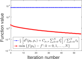
(a)

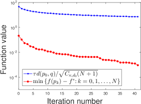
(b)

Figure 1: Iteration-complexity bound for the Riemannian subgradient method with: (a) exogenous step-size applied to Example 1 – Theorem 2; (b) Polyak’s step-size applied to Example 2 – Theorem 4.

As can be seen in Figure 1, inequalities (9) and (15) in Theorems 3 and 5 are met for all iterations of Algorithm 1, illustrating the practical reliability of our iteration-complexity results.

5 Conclusion

In this paper, we analyzed the iteration-complexity of subgradient method with exogenous step-size and Polyak’s step-size. In general, the Polyak’s step-size has a better performance than the exogenous step-size, but the choice of exogenous step-size is also interesting because it does not depend on any data computed during the algorithm, being important in large scale optimization problems. Since the feasibility and optimization problems are closed related, this paper complements the understanding of the subgradient algorithm in this settings. Finally, we remark that for Riemannian manifolds with curvature unbounded below, perhaps another strategy for the step will be need since is not possible to control the distance between the geodesics. Indeed, if the curvature is positive the geodesics emanating from the same point tend to approximate one each other, the contrary occurs if the curvature is negative.

References

- [1] G. C. Bento and J. X. Cruz Neto. A subgradient method for multiobjective optimization on Riemannian manifolds. J. Optim. Theory Appl., 159(1):125–137, 2013.
- [2] G. C. Bento, O. P. Ferreira, and J. G. Melo. Iteration-Complexity of Gradient, Subgradient and Proximal Point Methods on Riemannian Manifolds. J. Optim. Theory Appl., 173(2):548–562, 2017.
- [3] G. C. Bento, O. P. Ferreira, and P. R. Oliveira. Proximal point method for a special class of nonconvex functions on Hadamard manifolds. Optimization, 64(2):289–319, 2015.
- [4] G. C. Bento and J. G. Melo. Subgradient method for convex feasibility on Riemannian manifolds. J. Optim. Theory Appl., 152(3):773–785, 2012.
- [5] R. Burachik, L. M. G. Drummond, A. N. Iusem, and B. F. Svaiter. Full convergence of the steepest descent method with inexact line searches. Optimization, 32(2):137–146, 1995.
- [6] R. Correa and C. Lemaréchal. Convergence of some algorithms for convex minimization. Math. Programming, 62(2, Ser. B):261–275, 1993.
- [7] J. X. Da Cruz Neto, O. P. Ferreira, L. R. L. Pérez, and S. Z. Németh. Convex- and monotone-transformable mathematical programming problems and a proximal-like point method. J. Global Optim., 35(1):53–69, 2006.
- [8] M. P. do Carmo. Riemannian geometry. Mathematics: Theory & Applications. Birkhäuser Boston, Inc., Boston, MA, 1992. Translated from the second Portuguese edition by Francis Flaherty.
- [9] A. Edelman, T. A. Arias, and S. T. Smith. The geometry of algorithms with orthogonality constraints. SIAM J. Matrix Anal. Appl., 20(2):303–353, 1999.
- [10] O. P. Ferreira, A. N. Iusem, and S. Z. Németh. Concepts and techniques of optimization on the sphere. TOP, 22(3):1148–1170, 2014.
- [11] O. P. Ferreira, M. S. Louzeiro, and L. F. Prudente. Gradient Method for Optimization on Riemannian Manifolds with Lower Bounded Curvature. ArXiv e-prints, June 2018.
- [12] O. P. Ferreira and P. R. Oliveira. Subgradient algorithm on Riemannian manifolds. J. Optim. Theory Appl., 97(1):93–104, 1998.
- [13] J.-L. Goffin. Subgradient optimization in nonsmooth optimization (including the Soviet revolution). Doc. Math., (Extra vol.: Optimization stories):277–290, 2012.
- [14] P. Grohs and S. Hosseini. -subgradient algorithms for locally lipschitz functions on Riemannian manifolds. Adv. Comput. Math., 42(2):333–360, 2016.
- [15] S. Lang. Fundamentals of differential geometry, volume 191 of Graduate Texts in Mathematics. Springer-Verlag, New York, 1999.
- [16] C. Lenglet, M. Rousson, R. Deriche, and O. Faugeras. Statistics on the manifold of multivariate normal distributions: theory and application to diffusion tensor MRI processing. J. Math. Imaging Vision, 25(3):423–444, 2006.
- [17] C. Li, B. S. Mordukhovich, J. Wang, and J.-C. Yao. Weak sharp minima on Riemannian manifolds. SIAM J. Optim., 21(4):1523–1560, 2011.
- [18] C. Li and J.-C. Yao. Variational inequalities for set-valued vector fields on Riemannian manifolds: convexity of the solution set and the proximal point algorithm. SIAM J. Control Optim., 50(4):2486–2514, 2012.
- [19] D. G. Luenberger. The gradient projection method along geodesics. Management Sci., 18:620–631, 1972.
- [20] J. H. Manton. A framework for generalising the Newton method and other iterative methods from Euclidean space to manifolds. Numer. Math., 129(1):91–125, 2015.
- [21] Y. E. Nesterov and M. J. Todd. On the Riemannian geometry defined by self-concordant barriers and interior-point methods. Found. Comput. Math., 2(4):333–361, 2002.
- [22] B. T. Poljak. Subgradient methods: a survey of Soviet research. In Nonsmooth optimization (Proc. IIASA Workshop, Laxenburg, 1977), volume 3 of IIASA Proc. Ser., pages 5–29. Pergamon, Oxford-New York, 1978.
- [23] T. Rapcsák. Smooth nonlinear optimization in , volume 19 of Nonconvex Optimization and its Applications. Kluwer Academic Publishers, Dordrecht, 1997.
- [24] T. Sakai. Riemannian geometry, volume 149 of Translations of Mathematical Monographs. American Mathematical Society, Providence, RI, 1996. Translated from the 1992 Japanese original by the author.
- [25] S. T. Smith. Optimization techniques on Riemannian manifolds. In Hamiltonian and gradient flows, algorithms and control, volume 3 of Fields Inst. Commun., pages 113–136. Amer. Math. Soc., Providence, RI, 1994.
- [26] C. Udrişte. Convex functions and optimization methods on Riemannian manifolds, volume 297 of Mathematics and its Applications. Kluwer Academic Publishers Group, Dordrecht, 1994.
- [27] X. Wang, C. Li, J. Wang, and J.-C. Yao. Linear convergence of subgradient algorithm for convex feasibility on Riemannian manifolds. SIAM J. Optim., 25(4):2334–2358, 2015.
- [28] X. M. Wang. Subgradient algorithms on riemannian manifolds of lower bounded curvatures. Optimization, 67(1):179–194, 2018.
- [29] X. M. Wang, C. Li, and J. C. Yao. Subgradient projection algorithms for convex feasibility on Riemannian manifolds with lower bounded curvatures. J. Optim. Theory Appl., 164(1):202–217, 2015.
- [30] L. Yang. Riemannian median and its estimation. LMS J. Comput. Math., 13:461–479, 2010.
- [31] H. Zhang, S. J. Reddi, and S. Sra. Fast stochastic optimization on Riemannian manifolds. ArXiv e-prints, pages 1–17, 2016.
- [32] H. Zhang and S. Sra. First-order methods for geodesically convex optimization. JMLR: Workshop and Conference Proceedings, 49(1):1–21, 2016.