Study of $B_{s}\to\ell^{+}\ell^{-}\gamma$ decays in covariant quark model

Abstract

We study the rare radiative leptonic decays $B_{s}\to\ell^{+}\ell^{-}\gamma$ ($\ell=e,\mu,\tau$) within the Standard Model, considering both the structure-dependent amplitude and bremsstrahlung. In the framework of the covariant confined quark model developed by us, we calculate the form factors characterizing the $B_{s}\to\gamma$ transition in the full kinematical region of the dilepton momentum squared and discuss their behavior. We provide the analytic formula for the differential decay distribution and give predictions for the branching fractions in both cases: with and without long-distance contributions. Finally, we compare our results with those obtained in other approaches.

I   Introduction

The rare radiative decays $B_{q}\to\ell^{+}\ell^{-}\gamma$ with $\ell=e,\mu,\tau$ and $q=d,s$ are of great interest for several reasons. First, they are complementary to the well-known decays $B\to K^{(\ast)}\ell^{+}\ell^{-}$ and therefore provide us with extra tests of the Standard Model (SM) predictions for processes which proceed at loop level. Second, this process is not helicity suppressed as compared with the pure leptonic decays $B_{q}\to\ell^{+}\ell^{-}$ due to the appearance of a photon in the final state. Theoretical estimates of the decay branching fractions have shown that ${\cal B}\left(B_{s}\to\mu^{+}\mu^{-}\gamma\right)$ may be an order of magnitude larger than ${\cal B}\left(B_{s}\to\mu^{+}\mu^{-}\right)$.

There are a number of theoretical calculations of the branching fractions ${\cal B}(B_{q}\to\ell^{+}\ell^{-}\gamma)$ performed in different approaches. Among them one can mention the early studies in the framework of a constituent quark model Eilam:1996vg , light-cone QCD sum rules Aliev:1996ud ; Aliev:1997sd , and the light-front model Geng:2000fs . The structure-dependent amplitude of the decays $B_{s}\to\ell^{+}\ell^{-}\gamma$ was analyzed in Ref. Dincer:2001hu by taking a universal form for the form factors, which is motivated by QCD and related to the light-cone wave function of the $B_{s}$ meson. In Ref. Kruger:2002gf it was shown that efficient constraints on the behavior of the form factors can be obtained from the gauge-invariance requirement of the $B_{q}\to\ell^{+}\ell^{-}\gamma$ amplitude, as well as from the resonance structure of the form factors and their relations at large photon energies. Universality of nonperturbative QCD effects in radiative B decays was studied in Ref. DescotesGenon:2002ja . In Ref. Melikhov:2004mk long-distance QCD effects in the $B_{d/s}\to\ell^{+}\ell^{-}\gamma$ decays were analyzed. It was shown that the contribution of light vector-meson resonances related to the virtual photon emission from valence quarks of the $B$ meson gives a sizable impact on the dilepton differential distribution. In Ref. Kozachuk:2017mdk the $B_{d/s}\to\gamma$ transition form factors were calculated within the relativistic dispersion approach based on the constituent quark picture. A detailed analysis of the charm-loop contributions to the radiative leptonic decays was also performed. Very recently, a novel strategy to search for the decays $B_{s}\to\mu^{+}\mu^{-}\gamma$ in the event sample selected for $B_{s}\to\mu^{+}\mu^{-}$ searches was presented Dettori:2016zff .

It is worth noting that the predictions for the branching fractions $\mathcal{B}(B_{s}\to\ell^{+}\ell^{-}\gamma)$ given in the literature are still largely different from each other, ranging from $2.4\times 10^{-9}$ to $2.5\times 10^{-8}$ for the electron mode, and from $1.9\times 10^{-9}$ to $1.9\times 10^{-8}$ for the muon one Aliev:1996ud ; Melikhov:2004mk . Moreover, in some early calculations, the long-distance contributions from the $c\bar{c}$ resonances were neglected Eilam:1996vg ; Dincer:2001hu . Note that in Refs. Eilam:1996vg ; Aliev:1996ud ; Geng:2000fs the authors concluded that the contributions from diagrams with the virtual photon emitted from the valence quarks of the $B_{s}$ meson are small and therefore, neglected them. However, as we will show later on, the diagram with the virtual photon emission from the light $s$ quark gives a very sizable contribution.

Putting aside the total branching fraction, the shape of the hadronic form factors are important. In particular, it directly affects the decay distribution, and therefore the partial branching fraction integrated in different $q^{2}$ bins, which is more important for experimental studies than the total branching fraction. Regarding the form factor shape, the authors of Refs. Dincer:2001hu ; Kruger:2002gf have pointed out that the form factors $F_{TV}$ and $F_{TA}$ in Ref. Aliev:1996ud may be unreliable since they strongly violate the relation $F_{TV}\approx F_{TA}$ at large photon energies. Also, the form factors $F_{TV}$ and $F_{TA}$ obtained in Ref. Geng:2000fs vanish at maximum transferred momentum $q^{2}=m_{B_{s}}^{2}$, which seems unrealistic Kruger:2002gf . Among the model-based approaches, the most reliable form factors in the whole $q^{2}$ range are provided in Refs. Dincer:2001hu ; Kozachuk:2017mdk . However, in Ref. Dincer:2001hu , the resonances were not taken into account. Note that the light resonance $\phi$ is important since it significantly enhances the partial branching fraction in the low $q^{2}$ region, which is the main source of the signal for these decays at the LHC Melikhov:2004mk .

In the literature there exist also model-independent studies of the $B_{s}\to\ell^{+}\ell^{-}\gamma$ and related decays $B_{s}\to\ell^{+}\ell^{-}$ and $B_{s}\to\ell^{+}\nu_{\ell}\gamma$ DescotesGenon:2002ja ; Korchemsky:1999qb ; Lunghi:2002ju ; Bosch:2003fc ; Burdman:1994ip . However, most of them focus mainly on the form factors $F_{V}$ and $F_{A}$. Also, the form factors were given with high accuracy only in a limited kinematical range, usually the range where the photon energy $E_{\gamma}$ is much higher than the QCD scale. In Ref. Aditya:2012im , model-independent predictions for $\mathcal{B}(B_{s}\to\mu^{+}\mu^{-}\gamma)$ were provided, but only for the low-$E_{\gamma}$ region.

In this paper we calculate the matrix elements and the differential decay rates of the decays $B_{s}\to\ell^{+}\ell^{-}\gamma$ in the framework of the covariant confined quark model previously developed by us (see, e.g., Ref. Branz:2009cd ). This is a quantum-field theoretical model based on relativistic Lagrangians which effectively describe the interaction of hadrons with their constituent quarks. The quark confinement is realized by cutting the integration variable, which is called the proper time, at the upper limit. The interaction with the electromagnetic field is introduced by gauging the interaction Lagrangian in such a way as to keep the gauge invariance of the matrix elements at all calculation steps. This model has been successfully applied for the description of the matrix elements and form factors in the full kinematical region in semileptonic and rare decays of heavy mesons as well as baryons (see, e.g., Refs. Ivanov:2011aa ; Faessler:2002ut ; Dubnicka:2015iwg ; Gutsche:2015mxa ; Gutsche:2013pp ).

The rest of the paper is organized as follows. In Sec. II we give a necessary brief sketch of our approach. The introduction of electromagnetic interactions in the model is described in Sec. III. Section IV is devoted to the calculation of the decay matrix elements. We also briefly discuss their gauge invariance. In Sec. V we recalculate the formula for the twofold decay distribution in terms of the Mandelstam variables $(t,s)$. Then we integrate out the $t$ variable analytically and present the expression for the dilepton differential distribution. In Sec. VI we provide numerical results for the form factors, the differential decay widths, and the branching fractions. A comparison with existing results in the literature is included. Finally, we conclude in Sec. VII.

II   Brief sketch of the covariant confined quark model

The covariant confined quark model (CCQM) has been developed by our group in a series of papers. In this section, we mention several key elements of the model only for completeness. For a more detailed description of the model, as well as the calculation techniques used for the quark-loop evaluation, we refer to Refs. Branz:2009cd ; Ivanov:2011aa ; Faessler:2002ut ; Gutsche:2018nks ; Dubnicka:2015iwg ; Gutsche:2015mxa ; Gutsche:2013pp ; Ivanov:2015woa and references therein.

In the CCQM, the interaction Lagrangian of the $B_{s}$ meson with its constituent quarks is constructed from the hadron field $B_{s}(x)$ and the interpolating quark current $J_{B_{s}}(x)$:

$${\mathcal{L}_{\rm int}=g_{B_{s}}B_{s}(x)J_{B_{s}}(x)+H.c.},$$ (1)

where the latter is given by

$$J_{B_{s}}(x)=\int\!\!dx_{1}\!\!\int\!\!dx_{2}\>F_{B_{s}}(x;x_{1},x_{2})\bar{b}^{a}(x_{1})i\gamma_{5}s^{a}(x_{2}).$$ (2)

The hadron-quark coupling $g_{B_{s}}$ is obtained with the help of the compositeness condition, which requires the wave function renormalization constant of the hadron to be equal to zero $Z_{H}=0$. Here, $F_{B_{s}}(x;x_{1},x_{2})$ is the vertex function whose form is chosen so as to reflect the intuitive expectations about the relative quark-hadron positions

$$F_{B_{s}}(x;x_{1},x_{2})=\delta^{(4)}\left(x-w_{1}x_{1}-w_{2}x_{2}\right)\>\Phi_{B_{s}}\left[\left(x_{1}-x_{2}\right)^{2}\right],$$ (3)

where we require $w_{1}+w_{2}=1$. We actually adopt the most natural choice

$$w_{1}=\frac{m_{b}}{m_{b}+m_{s}},\qquad w_{2}=\frac{m_{s}}{m_{b}+m_{s}},$$ (4)

in which the barycenter of the hadron is identified with that of the quark system. The interaction strength $\Phi_{B_{s}}\left[\left(x_{1}-x_{2}\right)^{2}\right]$ is assumed to have a Gaussian form which is, in the momentum representation, written as

$$\widetilde{\Phi}_{B_{s}}\left(-p^{2}\right)=\exp\left(p^{2}/\Lambda_{B_{s}}^{2}\right).$$ (5)

Here, $\Lambda_{B_{s}}$ is a hadron-related size parameter, regarded as an adjustable parameter of the model. For the quark propagators $S_{q}$ we use the Fock-Schwinger representation

$$S_{q}(k)=(m_{q}+\not\!k)\int\limits_{0}^{\infty}\!d\alpha\exp[-\alpha(m_{q}^{2}-k^{2})].$$ (6)

Using various techniques described in our previous papers, a form factor $F$ can be finally written in the form of a threefold integral

$$F=\int\limits_{0}^{1/\lambda^{2}}\!\!dt\,t\!\!\int\limits_{0}^{1}\!\!d\alpha_{1}\!\!\int\limits_{0}^{1}\!\!d\alpha_{2}\,\delta\Big{(}1-\alpha_{1}-\alpha_{2}\Big{)}f(t\alpha_{1},t\alpha_{2}),$$ (7)

where $f(t\alpha_{1},t\alpha_{2})$ is the resulting integrand corresponding to the form factor $F$, and $\lambda$ is the so-called infrared cutoff parameter, which is introduced to avoid the appearance of the branching point corresponding to the creation of free quarks, and taken to be universal for all physical processes. The threefold integral in Eq. (7) is calculated by using fortran code with the NAG library.

The model parameters are determined from a least-squares fit to available experimental data and some lattice calculations. We have observed that the errors of the fitted parameters are within 10$\%$. We calculated the propagation of these errors on the form factors and found the uncertainties for the form factors to be of order 20$\%$ at small $q^{2}$ and 30$\%$ at high $q^{2}$ Soni:2018adu .

In this paper we use the results of the updated fit performed in Refs. Gutsche:2015mxa ; Ganbold:2014pua ; Issadykov:2015iba . The central values of the model parameters involved in this paper are given by (in GeV)

 0.241 0.428 1.67 5.04 0.181 2.05.fragments  0.241 0.428 1.67 5.04 0.181 2.05\begin{tabular}[]{ c c c c c c }\quad$m_{u/d}$&\quad$m_{s}$&\quad$m_{c}$&\quad$m_{b}$&\quad$\lambda$&\quad$\Lambda_{B_{s}}$\\ \hline\cr\quad 0.241&\quad 0.428&\quad 1.67&\quad 5.04&\quad 0.181&\quad 2.05\end{tabular}.

 m/ud  ms  mc  mb  λ  ΛBs  m/ud  ms  mc  mb  λ  ΛBs (8)

III   Electromagnetic interactions

Within the CCQM framework, interactions with electromagnetic fields are introduced as follows. First, one gauges the free-quark Lagrangian in the standard manner by using minimal substitution

$$\partial^{\mu}q_{i}\to(\partial^{\mu}-ie_{q_{i}}A^{\mu})q_{i}$$ (9)

that gives the quark-photon interaction Lagrangian

$${\cal L}^{\rm em-min}_{\rm int}(x)=\sum\limits_{q}e_{q}\bar{q}(x)\!\not\!\!A(x)q(x).$$ (10)

In order to guarantee local invariance of the strong interaction Lagrangian, one multiplies each quark field $q(x_{i})$ in ${\cal L}_{\rm int}^{\rm str}$ with a gauge field exponential. One then has

$$q_{i}(x_{i})\to e^{-ie_{q_{i}}I(x_{i},x,P)}q_{i}(x_{i}),$$ (11)

where

$$I(x_{i},x,P)=\int\limits_{x}^{x_{i}}dz_{\mu}A^{\mu}(z).$$ (12)

The path $P$ connects the end points of the path integral.

It is readily seen that the full Lagrangian is invariant under the transformations

$$q_{i}(x) \to e^{ie_{q_{i}}f(x)}q_{i}(x),$$

$$\bar{q}_{i}(x) \to \bar{q}_{i}(x)e^{-ie_{q_{i}}f(x)},$$ (13)

$$A^{\mu}(x) \to A^{\mu}(x)+\partial^{\mu}f(x).$$

One then expands the gauge exponential up to the required power of $e_{q}A_{\mu}$ needed in the perturbative series. This will give rise to a second term in the nonlocal electromagnetic interaction Lagrangian ${\cal L}^{\rm em-nonloc}_{\rm int}$. At first glance, it seems that the results will depend on the path $P$ taken to connect the end points of the path integral in Eq. (12). However, one needs to know only the derivatives of the path integral expressions when calculating the perturbative series. Therefore, we use the formalism suggested in Refs. Mandelstam:1962mi ; Terning:1991yt , which is based on the path-independent definition of the derivative of $I(x,y,P)$:

$$\frac{\partial}{\partial x^{\mu}}I(x,y,P)=A_{\mu}(x).$$ (14)

As a result of this rule, the Lagrangian describing the nonlocal interaction of the $B_{s}$ meson, the quarks, and electromagnetic fields reads (to the first order in the electromagnetic charge)

$${\cal L}^{\rm em-nonloc}_{\rm int}(x) = ig_{B_{s}}B_{s}(x)\int dx_{1}\int dx_{2}\int dz\left(\bar{b}(x_{1})\gamma_{5}s(x_{2})\right)A_{\mu}(z)E^{\mu}(x;x_{1},x_{2},z),$$ (15)

$$E^{\mu}(x;x_{1},x_{2},z) = \int\frac{d^{4}p_{1}}{(2\pi)^{4}}\int\frac{d^{4}p_{2}}{(2\pi)^{4}}\int\frac{d^{4}q}{(2\pi)^{4}}\exp[-ip_{1}(x_{1}-x)+ip_{2}(x_{2}-x)+iq(z-x)]$$ (16)

$$\times\Big{\{}e_{b}(q^{\mu}w_{2}-2p^{\mu})w_{2}\int\limits_{0}^{1}d\tau\tilde{\Phi}_{B_{s}}^{\prime}\left[-(p-w_{2}q)^{2}\tau-p^{2}(1-\tau)\right]$$

$$-e_{s}(q^{\mu}w_{1}+2p^{\mu})w_{1}\int\limits_{0}^{1}d\tau\tilde{\Phi}_{B_{s}}^{\prime}\left[-(p+w_{1}q)^{2}\tau-p^{2}(1-\tau)\right]\Big{\}},$$

where $p=w_{2}p_{1}+w_{1}p_{2}$.

IV   Matrix elements of the decays $B_{s}\to\ell^{+}\ell^{-}\gamma$

The decays $B_{s}\to\ell^{+}\ell^{-}\gamma$ are described by three sets of diagrams shown in Figs. 1–3. Diagrams from the first set (Fig. 1) correspond to the case when the real photon is emitted from the quarks or the meson-quark vertex.

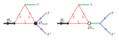
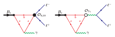
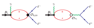
Figure 1: Diagrams which contribute to the decays $B_{s}\to\ell^{+}\ell^{-}\gamma$ with the real photon emitted from the quarks or the meson-quark vertex.

The effective Hamiltonian describing the $b\to s\ell^{+}\ell^{-}$ weak transition is written as

$${\mathcal{H}}_{\rm eff}^{b\to s\ell^{+}\ell^{-}} = \frac{G_{F}}{\sqrt{2}}\frac{\alpha_{\rm em}}{2\pi}\lambda_{t}\Big{[}C_{9}^{\rm eff}\left(\bar{s}\gamma^{\mu}(1-\gamma_{5})b\right)\left(\bar{\ell}\gamma_{\mu}\ell\right)$$ (17)

$$- \frac{2\tilde{m}_{b}}{q^{2}}C_{7}^{\rm eff}\left(\bar{s}i\sigma^{\mu\nu}q_{\nu}(1+\gamma_{5})b\right)\left(\bar{\ell}\gamma_{\mu}\ell\right)$$

$$+ C_{10}\left(\bar{s}\gamma^{\mu}(1-\gamma_{5})b\right)\left(\bar{\ell}\gamma_{\mu}\gamma_{5}\ell\right)\Big{]},$$

where $\lambda_{t}=V_{tb}V^{\ast}_{ts}$, and $\tilde{m}_{b}$ is the QCD quark mass which is different from the constituent quark mass $m_{b}$ used in our model. Here and in the following we denote the QCD quark masses with a tilde to distinguish them from the constituent quark masses used in the model [see Eq. (8)]. The Wilson coefficients $C_{7}^{\rm eff}=C_{7}-C_{5}/3-C_{6}$ and $C_{10}$ depend on the scale parameter $\mu$. The Wilson coefficient $C_{9}^{\rm eff}$ effectively takes into account, first, the contributions from the four-quark operators $\mathcal{O}_{i}$ ($i=1,...,6$) and, second, nonperturbative effects coming from the $c\bar{c}$-resonance contributions which are as usual parametrized by the Breit-Wigner ansatz Ali:1991is :

$$C_{9}^{\rm eff} = C_{9}+C_{0}\left\{h(\hat{m}_{c},s)+\frac{3\pi}{\alpha^{2}}\kappa\sum\limits_{V_{i}=\psi(1s),\psi(2s)}\frac{\Gamma(V_{i}\rightarrow\ell^{+}\ell^{-})m_{V_{i}}}{{m_{V_{i}}}^{2}-q^{2}-im_{V_{i}}\Gamma_{V_{i}}}\right\}$$ (18)

$$-\frac{1}{2}h(1,s)\left(4C_{3}+4C_{4}+3C_{5}+C_{6}\right)$$

$$-\frac{1}{2}h(0,s)\left(C_{3}+3C_{4}\right)+\frac{2}{9}\left(3C_{3}+C_{4}+3C_{5}+C_{6}\right),$$

where $C_{0}\equiv 3C_{1}+C_{2}+3C_{3}+C_{4}+3C_{5}+C_{6}$, $\hat{m}_{c}=\tilde{m}_{c}/M_{B_{s}}$, $s=q^{2}/M_{B_{s}}^{2}$, and $\kappa=1/C_{0}$. Here,

$$h(\hat{m}_{c},s) = -\frac{8}{9}\ln\frac{\tilde{m}_{b}}{\mu}-\frac{8}{9}\ln\hat{m}_{c}+\frac{8}{27}+\frac{4}{9}x$$ (21)

$$-\frac{2}{9}(2+x)|1-x|^{1/2}\left\{\begin{array}[]{ll}\left(\ln\left|\frac{\sqrt{1-x}+1}{\sqrt{1-x}-1}\right|-i\pi\right),&\mbox{for }x\equiv\frac{4\hat{m}_{c}^{2}}{s}<1,\\ &\\ 2\arctan\frac{1}{\sqrt{x-1}},&\mbox{for }x\equiv\frac{4\hat{m}_{c}^{2}}{s}>1,\end{array}\right.$$

$$h(0,s) = \frac{8}{27}-\frac{8}{9}\ln\frac{\tilde{m}_{b}}{\mu}-\frac{4}{9}\ln s+\frac{4}{9}i\pi.$$

The SM Wilson coefficients are taken from Ref. Descotes-Genon:2013vna . They were computed at the matching scale $\mu_{0}=2M_{W}$ and run down to the hadronic scale $\mu_{b}=4.8$ GeV. Their numerical values are given in Table 1.

Table 1: NNLO Wilson coefficients at the scale $\mu_{b}=4.8$ GeV obtained in Ref. Descotes-Genon:2013vna .

$C_{1}$	$C_{2}$	$C_{3}$	$C_{4}$	$C_{5}$	$C_{6}$	$C^{\rm eff}_{7}$	$C_{9}$	$C_{10}$
$-0.2632$	$1.0111$	$-0.0055$	$-0.0806$	0.0004	0.0009	$-0.2923$	4.0749	$-4.3085$

We use the bare $c$-quark mass corresponding to the “running” mass $\tilde{m}_{c}=\bar{m}_{c}(\mu~{}=\bar{m}_{c})=1.27\pm 0.03$ GeV in the $\overline{MS}$ scheme (for a review, see “Quark masses” in PDG Tanabashi:2018oca ). Note that the $\tilde{m}_{c}$ appears only in the charm-loop function $h(\hat{m}_{c},s)$ via the logarithm. Therefore, uncertainties related to the choice of the scale parameter $\mu$ are small. For the bare $b$-quark mass we use the central value of $\tilde{m}_{b}=m^{1S}_{b}=4.68\pm 0.03$ GeV obtained in the $1S$ mass scheme; see Ref. Bauer:2004ve . This value is close to the pole b-mass which was used in the Wilson coefficients $C_{i}(\mu_{b}).$ Finally, the values of $\alpha_{\rm em}(M_{Z})=1/128.94$ and $\lambda_{t}=|V_{tb}V^{\ast}_{ts}|=0.040$ are taken from PDG Tanabashi:2018oca .

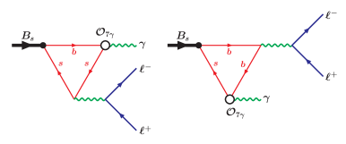
Figure 2: Diagrams which contribute to the decays $B_{s}\to\ell^{+}\ell^{-}\gamma$ with the real photon emitted from the penguin.

Diagrams from the second set (Fig. 2) represent the case when the real photon is emitted from the magnetic penguin operator. The effective Hamiltonian describing the $b\to s\gamma$ electroweak transition is written as

$${\mathcal{H}}_{\rm eff}^{b\to s\gamma}=-\frac{G_{F}}{\sqrt{2}}\lambda_{t}C_{7}^{\rm eff}\frac{e\tilde{m}_{b}}{8\pi^{2}}\left(\bar{s}\sigma_{\mu\nu}(1+\gamma_{5})b\right)F^{\mu\nu}.$$ (22)

Diagrams from the first two sets contribute to the structure-dependent (SD) part of the decay amplitude. They can be parametrized by a set of invariant form factors. In order to define the form factors, we specify our choice for the momenta in the decays as follows:

$$B_{s}(p_{1})\to\gamma(p_{2})+\ell^{+}(k_{+})+\ell^{-}(k_{-}),$$ (23)

where $p_{1}=p_{2}+k_{+}+k_{-}$ and $p_{1}-p_{2}=k_{+}+k_{-}\equiv q$, with $p_{1}^{2}=M^{2}_{B_{s}}$, $p_{2}^{2}=0$, $\epsilon^{\dagger}_{2}\cdot p_{2}=0$, and $k_{+}^{2}=k_{-}^{2}=m_{\ell}^{2}$.

We will use the definition of the $B_{s}\to\gamma$ transition form factors given, for instance, in Ref. Melikhov:2004mk :

$$\langle\gamma(p_{2},\epsilon_{2})|\bar{s}\gamma^{\mu}b|B_{s}(p_{1})\rangle = e\epsilon_{2\alpha}^{\dagger}\varepsilon^{\mu\alpha p_{1}p_{2}}\frac{F_{V}(q^{2})}{M_{B_{s}}},$$

$$\langle\gamma(p_{2},\epsilon_{2})|\bar{s}\gamma^{\mu}\gamma_{5}b|B_{s}(p_{1})\rangle = ie\epsilon_{2\alpha}^{\dagger}(g^{\mu\alpha}p_{1}p_{2}-p_{1}^{\alpha}p_{2}^{\mu})\frac{F_{A}(q^{2})}{M_{B_{s}}},$$

$$\langle\gamma(p_{2},\epsilon_{2})|\bar{s}\sigma^{\mu q}b|B_{s}(p_{1})\rangle = ie\epsilon_{2\alpha}^{\dagger}\varepsilon^{\mu\alpha p_{1}p_{2}}F_{TV}(q^{2}),$$

$$\langle\gamma(p_{2},\epsilon_{2})|\bar{s}\sigma^{\mu q}\gamma_{5}b|B_{s}(p_{1})\rangle = e\epsilon_{2\alpha}^{\dagger}(g^{\mu\alpha}p_{1}p_{2}-p_{1}^{\alpha}p_{2}^{\mu})F_{TA}(q^{2}).$$ (24)

Here we use the short notations $\sigma^{\mu q}\equiv\sigma^{\mu\beta}q_{\beta}$ and $\varepsilon^{\mu\alpha p_{1}p_{2}}\equiv\varepsilon^{\mu\alpha\beta\delta}p_{1\beta}p_{2\delta}$.

The form factors gain contributions from the diagrams in Figs. 1 and 2 in the following manner:

$$F_{V} = M_{B_{s}}\left[e_{b}\tilde{F}_{V}^{b\gamma b}+e_{s}\tilde{F}_{V}^{s\gamma s}\right],$$

$$F_{A} = M_{B_{s}}\left[e_{b}\tilde{F}_{A}^{b\gamma b}+e_{s}\tilde{F}_{A}^{s\gamma s}+e_{b}\tilde{F}_{A}^{{\rm bubble}-b}+e_{s}\tilde{F}_{A}^{{\rm bubble}-s}\right],$$

$$F_{TV} = e_{b}\tilde{F}_{TV}^{b\gamma b}+e_{s}\tilde{F}_{TV}^{s\gamma s}+e_{b}\tilde{F}_{TV}^{b(\bar{\ell}\ell)b}+e_{s}\tilde{F}_{TV}^{s(\bar{\ell}\ell)s},$$

$$F_{TA} = e_{b}\tilde{F}_{TA}^{b\gamma b}+e_{s}\tilde{F}_{TA}^{s\gamma s}+e_{b}\tilde{F}_{TA}^{{\rm bubble}-b}+e_{s}\tilde{F}_{TA}^{{\rm bubble}-s}+e_{b}\tilde{F}_{TA}^{b(\bar{\ell}\ell)b}+e_{s}\tilde{F}_{TA}^{s(\bar{\ell}\ell)s}.$$ (25)

The process with the virtual photon emitted from the light $s$ quark is described by the diagram in Fig. 2 (left panel). The physical region for $q^{2}$ in the decays $B_{s}\to\gamma\ell^{+}\ell^{-}$ is extended up to $q^{2}_{\rm max}=M^{2}_{B_{s}}$, which is much higher than the branch-point value $q^{2}=4m_{s}^{2}$. In this case, the form factor $\tilde{F}_{TV/TA}^{s(\bar{\ell}\ell)s}$ cannot be directly calculated in our model due to the appearance of hadronic singularities associated with the light vector meson resonances. In order to describe this amplitude, we follow the authors of Ref. Kozachuk:2017mdk in using the gauge-invariant version Melikhov:2003hs of the vector meson dominance Sakurai:1960ju ; GellMann:1961tg ; Gounaris:1968mw ,

$$\tilde{F}_{TV/TA}^{s(\bar{\ell}\ell)s}(q^{2})=\tilde{F}_{TV/TA}^{s(\bar{\ell}\ell)s}(0)-\sum\limits_{V}2f_{V}^{\rm e.m.}G^{T}_{1}(0)\frac{q^{2}/M_{V}}{q^{2}-M_{V}^{2}+iM_{V}\Gamma_{V}},$$ (26)

where $\Gamma_{V}$ and $M_{V}$ are the decay width and mass of the vector meson resonance, and $G^{T}_{1}(0)$ is one of the tensor form factors for the $B_{s}\to V$ transition, defined as follows Ivanov:2016qtw ; Ivanov:2017hun ; Tran:2018kuv :

$$\langle V(p_{2},\epsilon_{2})|\bar{s}\sigma^{\mu\nu}b|B_{s}(p_{1})\rangle=\epsilon^{\dagger}_{2\alpha}\Big{[}\varepsilon^{P\mu\nu\alpha}G_{1}^{T}(q^{2})+\varepsilon^{q\mu\nu\alpha}G_{2}^{T}(q^{2})+\varepsilon^{Pq\mu\nu}P^{\alpha}\frac{G_{0}^{T}(q^{2})}{(M_{B_{s}}+M_{V})^{2}}\Big{]}.$$ (27)

All parameters necessary for the form factor definition in Eq. (26) are calculated in our model and are given by

 0.120 0.227 0.266.fragments  0.120 0.227 0.266\begin{tabular}[]{ l c c }$\tilde{F}_{TV/TA}^{s(\bar{\ell}\ell)s}(0)$&\quad$f_{\phi}$ (GeV)&\quad$G_{1}^{T}(0)$\\ \hline\cr\quad 0.120&\quad 0.227&\quad 0.266\end{tabular}.

~F/TVTAs(¯ℓℓ)s(0) fϕ (GeV) G1T(0) ~F/TVTAs(¯ℓℓ)s(0) fϕ (GeV) G1T(0) (28)

Note that the electromagnetic decay constant is related to the leptonic decay constant by the relation $f_{\phi}^{\rm e.m.}=-\frac{1}{3}f_{\phi}$. Regarding the light resonances, here we consider only the main contribution from the ground-state $\phi$ meson. It is interesting to note that our result for $G_{1}^{T}(0)$ is equal to the value $0.27\pm 0.01$ obtained by the authors of Ref. Kozachuk:2017mdk .

Finally, the SD part of the amplitude is written in terms of the form factors as follows:

$$\mathcal{M}_{\rm SD} = \frac{G_{F}}{\sqrt{2}}\frac{\alpha_{\rm em}\lambda_{t}}{2\pi}e\epsilon^{\ast}_{2\alpha}\Big{\{}\Big{[}\varepsilon^{\mu\alpha p_{1}p_{2}}\frac{F_{V}(q^{2})}{M_{B_{s}}}-iT_{1}^{\mu\alpha}\frac{F_{A}(q^{2})}{M_{B_{s}}}\Big{]}\left(C_{9}^{\rm eff}\bar{\ell}\gamma_{\mu}\ell+C_{10}\bar{\ell}\gamma_{\mu}\gamma_{5}\ell\right)$$ (29)

$$\phantom{\frac{G_{F}}{\sqrt{2}}\frac{\alpha_{\rm em}\lambda_{t}}{2\pi}e\epsilon_{2\alpha}}+\Big{[}\varepsilon^{\mu\alpha p_{1}p_{2}}F_{TV}(q^{2})-iT_{1}^{\mu\alpha}F_{TA}(q^{2})\Big{]}\frac{2\tilde{m}_{b}}{q^{2}}C_{7}^{\rm eff}\bar{\ell}\gamma_{\mu}\ell\Big{\}},$$

where $T_{1}^{\mu\alpha}\equiv(g^{\mu\alpha}p_{1}p_{2}-p_{1}^{\alpha}p_{2}^{\mu})$.

The structure-independent part of the amplitude (bremsstrahlung) is described by the diagrams in Fig. 3.

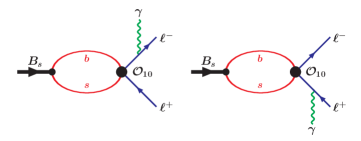
Figure 3: Bremsstrahlung diagrams.

Only the operator $\mathcal{O}_{10}$ contributes to this process, and it effectively gives the leptonic decay constant $f_{Bs}$. One has

$$\mathcal{M}_{\rm BR}=-i\frac{G_{F}}{\sqrt{2}}\frac{\alpha_{\rm em}\lambda_{t}}{2\pi}e\epsilon^{\ast}_{2\alpha}(2m_{\ell}f_{Bs}C_{10})\bar{u}({\boldmath{k_{-}}})\Big{[}\frac{\gamma^{\alpha}\not\!p_{1}}{t-m^{2}_{\ell}}-\frac{\not\!p_{1}\gamma^{\alpha}}{u-m^{2}_{\ell}}\Big{]}\gamma_{5}v({\boldmath{k_{+}}}).$$ (30)

Here, $t=(p_{2}+k_{-})^{2}=(p_{1}-k_{+})^{2}$, $u=(p_{2}+k_{+})^{2}=(p_{1}-k_{-})^{2}$, and $s=q^{2}$ so that $s+t+u=M_{B_{s}}^{2}+2m^{2}_{\ell}$. The variable $t$ varies in the interval $t_{-}\leq t\leq t_{+}$, where the bounds $t_{\pm}$ are given by

$$t_{\pm}=m^{2}_{\ell}+\frac{1}{2}(M_{B_{s}}^{2}-s)[1\pm\beta(s)],\qquad\beta(s)=\sqrt{1-\frac{4m^{2}_{\ell}}{s}}.$$ (31)

One can see that $t_{\pm}=m^{2}_{\ell}$ at minimum recoil $s=q^{2}=M_{B_{s}}^{2}$, which leads to the infrared pole in Eq. (30). A cut in the photon energy is required. In the $B_{s}$ center-of-mass system one has

$$E_{\gamma}=\frac{M_{B_{s}}}{2}\left(1-\frac{q^{2}}{M_{B_{s}}^{2}}\right)\geq E_{\gamma\,\rm min}.$$ (32)

Note that there are also weak annihilation diagrams with a $u(c)$ anomalous triangle in addition to the above diagrams. However, the contribution from these diagrams is much smaller than that from other diagrams as was shown in Ref. Melikhov:2004mk . Therefore, we will drop these types of diagrams in what follows.

A few remarks should be made with respect to the calculation of the Feynman diagrams in our approach. The SD part of the matrix element is described by the diagrams in Figs. 1 and 2. These diagrams do not include ultraviolet divergences because the hadron-quark vertex functions drop off exponentially in the Euclidean region. The loop integration is performed by using the Fock-Schwinger representation for the quark propagators, and the exponential form for the meson-quark vertex functions. The tensorial integrals are calculated by using the differential technique. The final expression for the SD part is represented as a sum of products of Lorentz structures and the corresponding invariant form factors. The form factors are described by threefold integrals in such a way that one integration is over a dimensional parameter $t$ (proper time), which proceeds from zero to infinity, and two others are over dimensionless Schwinger parameters. The possible branch points and cuts are regularized by introducing the cutoff at the upper limit of the integration over proper time. The final integrals are calculated numerically by using the fortran codes.

Then one can check that the final expression for the SD part of the amplitude is gauge invariant. Technically, it means that in addition to the gauge-invariant structures $\varepsilon^{\mu\alpha p_{1}p_{2}}$ and $T_{1}^{\mu\alpha}=(g^{\mu\alpha}p_{1}p_{2}-p_{1}^{\alpha}p_{2}^{\mu})$, the amplitude has also the non-gauge-invariant pieces $g^{\mu\alpha}$ and $p_{1}^{\mu}p_{1}^{\alpha}$. We have checked numerically that the form factors corresponding to the non-gauge-invariant part vanish for arbitrary momentum transfer squared $q^{2}$.

V   Differential decay rate

The twofold decay distribution is written as

$$\frac{d\Gamma}{dsdt}=\frac{1}{2^{8}\pi^{3}M_{B_{s}}^{3}}\sum_{\rm pol}|\mathcal{M}|^{2},\qquad\mathcal{M}=\mathcal{M}_{\rm SD}+\mathcal{M}_{\rm BR},$$ (33)

where $\sum_{\rm pol}$ denotes the summation over polarizations of both the photon and leptons. The physical region was discussed in the previous section, which reads $4m^{2}_{\ell}\leq s\equiv q^{2}\leq M_{B_{s}}^{2}$, and $t_{-}\leq t\leq t_{+}$. It is more convenient to write the final result for the twofold decay distribution in terms of dimensionless momenta and masses:

$$\hat{X}\equiv\frac{X}{M^{2}_{B_{s}}}\quad(X=s,t,u),\quad\hat{Y}\equiv\frac{Y}{M_{B_{s}}}\quad(Y=m_{\ell},\tilde{m}_{q},f_{B_{s}}),\quad\text{etc.}$$ (34)

The decay distribution is written as a sum of the SD part, the bremsstrahlung (BR), and the interference (IN) ones as follows:

$$\frac{d\Gamma}{d{\hat{s}}d{\hat{t}}}=N_{t}\Big{(}\frac{d\Gamma_{\rm SD}}{d{\hat{s}}d{\hat{t}}}+\frac{d\Gamma_{\rm BR}}{d{\hat{s}}d{\hat{t}}}+\frac{d\Gamma_{\rm IN}}{d{\hat{s}}d{\hat{t}}}\Big{)},\qquad N_{t}\equiv\frac{G_{F}^{2}\alpha_{\rm em}^{3}M_{B_{s}}^{5}|\lambda_{t}|^{2}}{2^{10}\pi^{4}}.$$ (35)

One has

$$\frac{d\Gamma_{\rm SD}}{d{\hat{s}}d{\hat{t}}} = {\hat{x}}^{2}B_{0}+{\hat{x}}({\hat{u}}-{\hat{t}})B_{1}+({\hat{u}}-{\hat{t}})^{2}B_{2},$$

$$B_{0}=({\hat{s}}+4{\hat{m}_{\ell}}^{2})\Delta F-8{\hat{m}_{\ell}}^{2}C_{10}^{2}(F_{V}^{2}+F_{A}^{2}),$$

$$B_{1}=8\big{[}{\hat{s}}C_{10}{\rm Re}(C^{\rm eff}_{9})F_{V}F_{A}+{\hat{m}_{b}}C_{7}^{\rm eff}C_{10}(F_{V}{\rm Re}(F_{TA})+F_{A}{\rm Re}(F_{TV}))\big{]},$$

$$B_{2}={\hat{s}}\Delta F,$$

$$\Delta F=(|C^{\rm eff}_{9}|^{2}+C_{10}^{2})(F_{V}^{2}+F_{A}^{2})+\Big{(}\frac{2{\hat{m}_{b}}}{{\hat{s}}}\Big{)}^{2}(C_{7}^{\rm eff})^{2}(|F_{TV}|^{2}+|F_{TA}|^{2})$$

$$\phantom{\Delta F=}+\Big{(}\frac{4{\hat{m}_{b}}}{{\hat{s}}}\Big{)}C_{7}^{\rm eff}[F_{V}{\rm Re}(C^{\rm eff}_{9}F_{TV})+F_{A}{\rm Re}(C^{\rm eff}_{9}F_{TA})],$$

$$\frac{d\Gamma_{\rm BR}}{d{\hat{s}}d{\hat{t}}} = (8{\hat{f}_{B_{s}}})^{2}{\hat{m}_{\ell}}^{2}C_{10}^{2}\Big{[}\frac{1}{2}(1+{\hat{s}}^{2})\hat{D}_{u}\hat{D}_{t}-({\hat{x}}{\hat{m}_{\ell}}\hat{D}_{u}\hat{D}_{t})^{2}\Big{]},$$ (37)

$$\frac{d\Gamma_{\rm IN}}{d{\hat{s}}d{\hat{t}}} = -16{\hat{f}_{B_{s}}}{\hat{m}_{\ell}}^{2}{\hat{x}}^{2}\hat{D}_{u}\hat{D}_{t}$$ (38)

$$\times\Big{[}\frac{2{\hat{x}}{\hat{m}_{b}}}{{\hat{s}}}C_{10}C_{7}^{\rm eff}{\rm Re}(F_{TV})+{\hat{x}}C_{10}{\rm Re}(C^{\rm eff}_{9})F_{V}+({\hat{u}}-{\hat{t}})C_{10}^{2}F_{A}\Big{]},$$

where ${\hat{x}}=1-{\hat{s}}$, $\hat{D}_{t}=1/({\hat{t}}-{\hat{m}_{\ell}}^{2})$, and $\hat{D}_{u}=1/({\hat{u}}-{\hat{m}_{\ell}}^{2})$. We have checked that all the expressions above are in agreement with those given in Ref. Kozachuk:2017mdk .

After integrating out the variable $\hat{t}$ we obtain the following analytic expressions for the differential decay rate:

$$\frac{d\Gamma_{\rm SD}}{d{\hat{s}}} = N_{t}{\hat{x}}^{3}\beta\big{[}B_{0}+\tfrac{1}{3}\beta^{2}B_{2}\big{]},$$ (39)

$$\frac{d\Gamma_{\rm BR}}{d{\hat{s}}} = N_{t}(8{\hat{f}_{B_{s}}})^{2}{\hat{m}_{\ell}}^{2}C^{2}_{10}\Big{[}\frac{1+{\hat{s}}^{2}}{{\hat{x}}}\ln\Big{(}\frac{1+\beta}{1-\beta}\Big{)}$$ (40)

$$\phantom{N_{t}(8{\hat{f}_{B_{s}}})^{2}{\hat{m}_{\ell}}^{2}C^{2}_{10}\Big{[}}-\frac{8{\hat{m}_{\ell}}^{2}}{{\hat{x}}}\Big{(}\frac{\beta}{1-\beta^{2}}+\tfrac{1}{2}\ln\Big{(}\frac{1+\beta}{1-\beta}\Big{)}\Big{)}\Big{]},$$

$$\frac{d\Gamma_{\rm IN}}{d{\hat{s}}} = -N_{t}32{\hat{f}_{B_{s}}}{\hat{m}_{\ell}}^{2}{\hat{x}}^{2}\ln\Big{(}\frac{1+\beta}{1-\beta}\Big{)}\Big{[}C_{10}{\rm Re}(C^{\rm eff}_{9})F_{V}+\frac{2{\hat{m}_{b}}}{{\hat{s}}}C_{7}^{\rm eff}C_{10}{\rm Re}(F_{TV})\Big{]},$$ (41)

where $\beta=\sqrt{1-4{\hat{m}_{\ell}}^{2}/{\hat{s}}}$.

VI   Numerical results

In Fig. 4 we present the $q^{2}$ dependence of the calculated form factors with the fixed values of the model parameters given in Eq. (8) in the full kinematical region $0\leq q^{2}\leq M^{2}_{B_{s}}$. Here, the form factors $\tilde{F}_{TV}$ and $\tilde{F}_{TA}$ are defined as follows:

$$\tilde{F}_{TV/TA}(q^{2})=F_{TV/TA}(q^{2})-e_{s}\tilde{F}_{TV/TA}^{s(\bar{l}l)s}.$$ (42)

One sees that $\tilde{F}_{TV}$ and $\tilde{F}_{TA}$ are real and are made of contributions from all diagrams except for the one with the virtual photon emitted from the $s$ quark. The total form factors $F_{TV}$ and $F_{TA}$ are complex due to the parametrization of $\tilde{F}_{TV/TA}^{s(\bar{l}l)s}$ in Eq. (26). In Fig. 4 (lower panels) we also plot the absolute values $|F_{TV}|$ and $|F_{TA}|$ together with $\tilde{F}_{TV}$ and $\tilde{F}_{TA}$ for comparison.

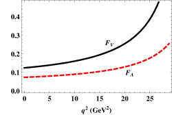
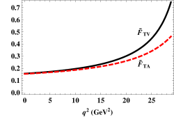
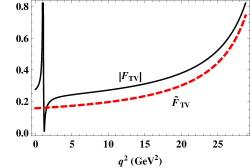
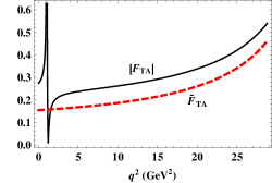
Figure 4: Form factors for the $B_{s}\to\gamma$ transition (see text for more details).

The results of our numerical calculations for the form factors $F_{V}$, $F_{A}$, $\tilde{F}_{TV}$, and $\tilde{F}_{TA}$ can be approximated with high accuracy by the double-pole parametrization

$$F(q^{2})=\frac{F(0)}{1-a\hat{s}+b\hat{s}^{2}},\qquad\hat{s}=\frac{q^{2}}{M_{B^{\ast}_{s}}^{2}},$$ (43)

with the relative error less than 1$\%$. The parameters $F(0)$, $a$, and $b$ are listed in Table 2. For completeness we also list here the values of the form factors at zero recoil $(q^{2}_{\rm max})$.

Table 2: Parameters of the approximated $B_{s}\rightarrow\gamma$ form factors and their values at zero recoil.

	$F_{V}$	$F_{A}$	$\tilde{F}_{TV}$	$\tilde{F}_{TA}$
$F(0)$	0.13	0.074	0.16	0.15
$a$	0.56	0.42	0.47	0.41
$b$	$-0.27$	$-0.31$	$-0.34$	$-0.27$
$F(q^{2}_{\rm max})$	0.67	0.26	0.74	0.46

In Figs. 5 we compare our form factors with the Kozachuk-Melikhov-Nikitin (KMN) form factors calculated in Ref. Kozachuk:2017mdk . Using the definitions in Eqs. (24) and (25) we can relate our form factors $F_{i}(q^{2})$ to the KMN form factors $F_{i}(q^{2},0)$ as follows (see Ref. Kozachuk:2017mdk for more detail):

$$F_{V/A}(q^{2},0)=F_{V/A}(q^{2}),\qquad F_{TV/TA}(q^{2},0)=F_{TV/TA}(q^{2})-e_{b}\tilde{F}_{TV/TA}^{b(\bar{l}l)b}-e_{s}\tilde{F}_{TV/TA}^{s(\bar{l}l)s}.$$ (44)

One can see that in the low-$q^{2}$ region ($q^{2}\lesssim 20$ GeV²) the corresponding form factors from the two sets are very close. In the high-$q^{2}$ region, the KMN form factors steeply increase and largely exceed our form factors.

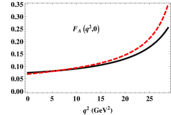
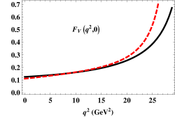
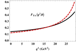
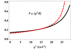
Figure 5: Comparison of the form factors $F_{i}(q^{2},0)$ calculated in our model (solid lines) with those from Ref. Kozachuk:2017mdk (dashed lines).

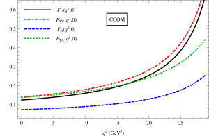
Figure 6: Behavior of the form factors $F_{i}(q^{2},0)$ in comparison with Ref. Kozachuk:2017mdk (KMN).

In order to have a better picture of the behavior of the form factors, in Fig. 6 we plot all of them together and compare with those from Ref. Kozachuk:2017mdk . It is very interesting to note that our form factors share with the corresponding KMN ones not only similar shapes (especially in the low-$q^{2}$ region) but also relative behaviors, i.e., similar relations between the form factors, in the whole $q^{2}$ region. Several comments should be made: (i) our form factors satisfy the constraint $F_{TA}(q^{2},0)=F_{TV}(q^{2},0)$ at $q^{2}=0$, with the common value equal to 0.135; (ii) in the small-$q^{2}$ region, $F_{V}(q^{2},0)\approx F_{TA}(q^{2},0)\approx F_{TV}(q^{2},0)$; (iii) $F_{V}(q^{2},0)$ and $F_{TV}(q^{2},0)$ are approximately equal in the full kinematical range and rise steeply in the high-$q^{2}$ region; and (iv) $F_{A}(q^{2},0)$ and $F_{TA}(q^{2},0)$ are rather flat when $q^{2}\to M_{B_{s}}^{2}$ as compared to $F_{V}(q^{2},0)$ and $F_{TV}(q^{2},0)$. These observations show that our form factors satisfy very well the constraints on their behavior proposed by the authors of Ref. Kruger:2002gf .

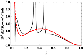
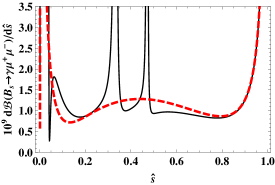
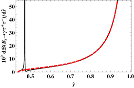
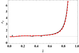
Figure 7: Differential branching fractions $10^{9}d\mathcal{B}\left(B_{s}\to\gamma\ell^{+}\ell^{-}\right)/d\hat{s}$ and ratio $r_{\gamma}$ as functions of the dimensionless variable $\hat{s}=q^{2}/M^{2}_{B_{s}}$ without long-distance contributions (dashed lines) and with contributions of the low lying charmonia $J/\psi$ and $\psi(2S)$, and the light $\phi$ meson (solid lines). The photon energy cut $E_{\gamma\,\rm min}=20$ MeV is used.

In Fig. 7 we plot the differential branching fractions $10^{9}d\mathcal{B}\left(B_{s}\to\gamma\ell^{+}\ell^{-}\right)/d\hat{s}$ as functions of the dimensionless variable $\hat{s}=q^{2}/M^{2}_{B_{s}}$. We also plot here the ratio

$$r_{\gamma}(\hat{s})\equiv\frac{d\mathcal{B}(B_{s}\to\gamma\mu^{+}\mu^{-})/d\hat{s}}{{d\mathcal{B}(B_{s}\to\gamma e^{+}e^{-})/d\hat{s}}},$$ (45)

which is a promising observable for testing lepton flavor universality (LFU) in these channels Guadagnoli:2017quo . The ratio $r_{\gamma}$ is very close to unity in the low-$q^{2}$ region but far above unity at large $q^{2}$ due to bremsstrahlung. As was pointed out in Ref. Kozachuk:2017mdk , in the high-$q^{2}$ region ($q^{2}\gtrsim 15$ GeV²), the ratio $r_{\gamma}$ is mainly described by the form factors $F_{A}(q^{2})$ and $F_{V}(q^{2})$. Therefore, knowledge of their behavior at large $q^{2}$ plays an important role in testing LFU. In Fig. 8 we plot the ratio $r_{\gamma}$ at large $q^{2}$ in comparison with Ref. Kozachuk:2017mdk . The ratios are very close in the range $16\lesssim q^{2}\lesssim 20$ GeV² (i.e., $0.55\lesssim\hat{s}\lesssim 0.69$), which is a result of the similarity between the form factors discussed above.

Figure 8: Ratio $r_{\gamma}(\hat{s})$ at large $\hat{s}$ obtained in our model (solid line) and from Ref. Kozachuk:2017mdk (dotted line).

The authors of Ref. Guadagnoli:2017quo suggested a useful observable

$$R_{\gamma}(\hat{s}_{1},\hat{s}_{2})\equiv\frac{\int_{\hat{s}_{1}}^{\hat{s}_{2}}d\hat{s}\,d\mathcal{B}(B_{s}\to\gamma\mu^{+}\mu^{-})/d\hat{s}}{{\int_{\hat{s}_{1}}^{\hat{s}_{2}}d\hat{s}\,d\mathcal{B}(B_{s}\to\gamma e^{+}e^{-})/d\hat{s}}},$$ (46)

with the optimal choice $\hat{s}_{1}=0.55$ and $\hat{s}_{2}=0.8$ (corresponding to $q^{2}_{1}=15.8$ GeV² and $q^{2}_{2}=23.0$ GeV², respectively). In this range, the ratio is dominated by the form factors $F_{A}(q^{2})$ and $F_{V}(q^{2})$. We provide our prediction for this ratio $R_{\gamma}(0.55,0.8)=1.54$, about $30\%$ larger than the prediction $R_{\gamma}(0.55,0.8)=1.115\pm 0.030$ given in Ref. Guadagnoli:2017quo . Note that from the results of Ref. Kozachuk:2017mdk , one obtains $R_{\gamma}(0.55,0.8)=1.32$.

In Table 3 we give the values of the branching fractions calculated without and with long-distance contributions. In the calculation with long-distance contributions, the region of two low lying charmonia is excluded by assuming $0.33\leq\hat{s}\leq 0.55$, as usually done in experimental data analysis. It is seen that the bremsstrahlung contribution to the electron mode is negligible, while for the tau mode it becomes the main part.

Table 3: Branching fractions with (in brackets) and without long-distance contributions. The used minimal photon energy is $E_{\gamma\,\rm min}=20$ MeV.

	SD	BR	IN	Sum
$10^{9}\mathcal{B}(B_{s}\to\gamma e^{+}e^{-})$	3.05 (15.9)	$3.2\times 10^{-5}$	$-4.8({\bf-9.5})\times 10^{-6}$	3.05 (15.9)
$10^{9}\mathcal{B}(B_{s}\to\gamma\mu^{+}\mu^{-})$	1.16 (10.0)	0.53	$-7.4({\bf-14.4})\times 10^{-3}$	1.7 (10.5)
$10^{9}\mathcal{B}(B_{s}\to\gamma\tau^{+}\tau^{-})$	0.10 (0.05)	13.4	0.30 (0.18)	13.8 (13.7)

In Table 4 we compare our results for the branching fractions with those obtained in other approaches. Our predictions for the electron and muon modes agree well with the results of Ref. Melikhov:2017pwu . In the case of the tau mode, the contribution from bremsstrahlung dominates the decay branching fractions and the SD amplitude becomes less important. As a result, our prediction for $\mathcal{B}(B_{s}\to\gamma\tau^{+}\tau^{-})$ agrees well with other studies.

Table 4: Comparison of the branching fractions $10^{9}\mathcal{B}(B_{s}\to\gamma\ell^{+}\ell^{-})$ ($\ell=e,\mu,\tau$) with other approaches. The used minimal photon energy is $E_{\gamma\,\rm min}=20$ MeV.

Reference	Electron	Muon	Tau
This work	15.9	10.5	13.7
Eilam:1996vg	6.2	4.6	$\dots$
Aliev:1996ud	2.35	1.9	$\dots$
Aliev:1997sd	$\dots$	$\dots$	15.2
Geng:2000fs	7.1	8.3	15.7
Dincer:2001hu	20.0	12.0	$\dots$
Melikhov:2004mk	24.6	18.9	11.6
Melikhov:2017pwu	18.4	11.6	$\dots$
Wang:2013rfa	17.4	17.4	$\dots$

Finally, in Tables 5 and 6 we provide our predictions for the branching fractions integrated over several $q^{2}$ bins, which are more practical for experimental studies than the total branching fractions. We show also the corresponding results obtained by KMN Kozachuk:2017mdk , and Guadagnoli-Reboud-Zwicky (GRZ) Guadagnoli:2017quo for comparison. It is seen that our predictions agree quite well with both the KMN and GRZ results.

Table 5: Branching fractions $10^{9}\Delta\mathcal{B}(B_{s}\to\gamma\ell^{+}\ell^{-})$ integrated in several $q^{2}$ bins. KMN results are given in brackets Kozachuk:2017mdk . Here, to obtain $q^{2}_{\rm max}$ we use $E_{\gamma\,{\rm min}}=80$ MeV [see Eq. (32)], which was also used in Ref. Kozachuk:2017mdk , in order to define the same bin.

	$\left[4m_{e}^{2},4m_{\mu}^{2}\right]$	$\left[4m_{\mu}^{2},1\,{\rm GeV}^{2}\right]$	$\left[1\,{\rm GeV}^{2},6\,{\rm GeV}^{2}\right]$	$\left[6\,{\rm GeV}^{2},0.33M_{B_{s}}^{2}\right]$	$\left[0.55M_{B_{s}}^{2},q^{2}_{\rm max}\right]$
$B_{s}\to\gamma e^{+}e^{-}$	5.76 (4.67)	2.24 (1.80)	7.50 (6.00)	0.28 (0.14)	0.17 (0.20)
$B_{s}\to\gamma\mu^{+}\mu^{-}$	$\dots$	2.05 (1.80)	7.50 (6.00)	0.29 (0.15)	0.47 (0.43)

Table 6: Branching fractions $10^{9}\Delta\mathcal{B}(B_{s}\to\gamma\mu^{+}\mu^{-})$ integrated in low and high $q^{2}$ regions. Here, we use $E_{\gamma\,{\rm min}}=50$ MeV as in Ref. Guadagnoli:2017quo , in order to define the same bin.

	$\left[4m_{\mu}^{2},\,0.30M_{B_{s}}^{2}\right]$	$\left[0.55M_{B_{s}}^{2},\,M_{B_{s}}^{2}-2E_{\gamma\,{\rm min}}M_{B_{s}}\right]$
This work	9.6	0.53
GRZ Guadagnoli:2017quo	$8.4\pm 1.3$	$0.89\pm 0.10$

Our predictions for the branching fractions in Tables 3–6 contain the uncertainties from the hadronic form factors and from other inputs, including the Wilson coefficients given in Table 1. However, the uncertainties from the latter are much smaller than those from the former. Therefore we estimate the errors of the branching fractions to be of order $30\%$ based on the uncertainty of the form factors.

It is also important to note that the light $\phi$ meson resonance significantly enhances the branching fractions of the electron and muon modes. In the calculation above we have integrated over the whole $q^{2}$ range corresponding to the $\phi$ meson resonance. If we consider a small $q^{2}$ cut $[(m_{\phi}-\Gamma_{\phi})^{2},(m_{\phi}+\Gamma_{\phi})^{2}]$ around the $\phi$ resonance, then we obtain $10^{9}\Delta\mathcal{B}(B_{s}\to\gamma\ell^{+}\ell^{-})=2.04$ for $q^{2}\in[1,6]\,{\rm GeV}^{2}$, where $\ell=e\,,\mu$.

VII   Summary and conclusions

We have studied the rare radiative leptonic decays $B_{s}\to\gamma\ell^{+}\ell^{-}$ ($\ell=e,\mu,\tau$) in the framework of the covariant confined quark model. The relevant transition form factors have been obtained in the full kinematical range of dilepton momentum transfer squared. We have found a very good agreement between our form factors and those from Ref. Kozachuk:2017mdk , especially in the region $q^{2}\lesssim 20$ GeV². We have provided predictions for the decay branching fractions and their ratio. The branching fractions for the light leptons agree well with the results of Ref. Melikhov:2017pwu . For the tau mode, our prediction agrees well with all existing values in the literature. The branching fractions in different $q^{2}$ bins have also been calculated, and show good agreement with the results of Refs. Kozachuk:2017mdk ; Guadagnoli:2017quo . In particular, we have predicted $10^{9}\Delta\mathcal{B}(B_{s}\to\gamma\ell^{+}\ell^{-})=7.50$ for $q^{2}\in[1,6]\,{\rm GeV}^{2}$, where $\ell=e\,,\mu$.

- (1) G. Eilam, C. D. Lu, and D. X. Zhang, Phys. Lett. B 391, 461 (1997) [hep-ph/9606444].
- (2) T. M. Aliev, A. Ozpineci, and M. Savci, Phys. Rev. D 55, 7059 (1997) [hep-ph/9611393].
- (3) T. M. Aliev, N. K. Pak, and M. Savci, Phys. Lett. B 424, 175 (1998) [hep-ph/9710304].
- (4) C. Q. Geng, C. C. Lih, and W. M. Zhang, Phys. Rev. D 62, 074017 (2000) [hep-ph/0007252].
- (5) Y. Dincer and L. M. Sehgal, Phys. Lett. B 521, 7 (2001) [hep-ph/0108144].
- (6) F. Krüger and D. Melikhov, Phys. Rev. D 67, 034002 (2003) [hep-ph/0208256].
- (7) S. Descotes-Genon and C. T. Sachrajda, Phys. Lett. B 557, 213 (2003) [hep-ph/0212162].
- (8) D. Melikhov and N. Nikitin, Phys. Rev. D 70, 114028 (2004) [hep-ph/0410146].
- (9) A. Kozachuk, D. Melikhov, and N. Nikitin, Phys. Rev. D 97, 053007 (2018) [arXiv:1712.07926].
- (10) F. Dettori, D. Guadagnoli, and M. Reboud, Phys. Lett. B 768, 163 (2017) [arXiv:1610.00629].
- (11) G. P. Korchemsky, D. Pirjol, and T. M. Yan, Phys. Rev. D 61, 114510 (2000) [hep-ph/9911427].
- (12) E. Lunghi, D. Pirjol, and D. Wyler, Nucl. Phys. B649, 349 (2003) [hep-ph/0210091].
- (13) S. W. Bosch, R. J. Hill, B. O. Lange, and M. Neubert, Phys. Rev. D 67, 094014 (2003) [hep-ph/0301123].
- (14) G. Burdman, J. T. Goldman, and D. Wyler, Phys. Rev. D 51, 111 (1995) [hep-ph/9405425].
- (15) Y. G. Aditya, K. J. Healey, and A. A. Petrov, Phys. Rev. D 87, 074028 (2013) [arXiv:1212.4166].
- (16) T. Branz, A. Faessler, T. Gutsche, M. A. Ivanov, J. G. Körner, and V. E. Lyubovitskij, Phys. Rev. D 81, 034010 (2010) [arXiv:0912.3710].
- (17) M. A. Ivanov, J. G. Körner, S. G. Kovalenko, P. Santorelli, and G. G. Saidullaeva, Phys. Rev. D 85, 034004 (2012) [arXiv:1112.3536].
- (18) A. Faessler, T. Gutsche, M. A. Ivanov, J. G. Körner, and V. E. Lyubovitskij, Eur. Phys. J. direct C 4, 18 (2002) [hep-ph/0205287].
- (19) S. Dubnička, A. Z. Dubničková, N. Habyl, M. A. Ivanov, A. Liptaj, and G. S. Nurbakova, Few-Body Syst. 57, 121 (2016) [arXiv:1511.04887].
- (20) T. Gutsche, M. A. Ivanov, J. G. Körner, V. E. Lyubovitskij, P. Santorelli, and N. Habyl, Phys. Rev. D 91, 074001 (2015); 91, 119907(E) (2015) [arXiv:1502.04864].
- (21) T. Gutsche, M. A. Ivanov, J. G. Körner, V. E. Lyubovitskij, and P. Santorelli, Phys. Rev. D 87, 074031 (2013) [arXiv:1301.3737].
- (22) M. A. Ivanov and C. T. Tran, Phys. Rev. D 92, 074030 (2015) [arXiv:1701.07377].
- (23) T. Gutsche, M. A. Ivanov, J. G. Körner, V. E. Lyubovitskij, P. Santorelli, and C. T. Tran, Phys. Rev. D 98, 053003 (2018) [arXiv:1807.11300].
- (24) G. Ganbold, T. Gutsche, M. A. Ivanov, and V. E. Lyubovitskij, J. Phys. G 42, 075002 (2015) [arXiv:1410.3741].
- (25) A. Issadykov, M. A. Ivanov, and S. K. Sakhiyev, Phys. Rev. D 91, 074007 (2015), [arXiv:1502.05280].
- (26) N. R. Soni, M. A. Ivanov, J. G. Körner, J. N. Pandya, P. Santorelli and C. T. Tran, Phys. Rev. D 98, no. 11, 114031 (2018) [arXiv:1810.11907 [hep-ph]].
- (27) S. Mandelstam, Ann. Phys. (Paris) 19, 1 (1962).
- (28) J. Terning, Phys. Rev. D 44, 887 (1991).
- (29) A. Ali, T. Mannel, and T. Morozumi, Phys. Lett. B 273, 505 (1991).
- (30) S. Descotes-Genon, T. Hurth, J. Matias, and J. Virto, J. High Energy Phys. 05 (2013) 137 [arXiv:1303.5794].
- (31) M. Tanabashi et al. (Particle Data Group), Phys. Rev. D 98, no. 3, 030001 (2018).
- (32) C. W. Bauer, Z. Ligeti, M. Luke, A. V. Manohar, and M. Trott, Phys. Rev. D 70, 094017 (2004) [hep-ph/0408002].
- (33) D. Melikhov, O. Nachtmann, V. Nikonov, and T. Paulus, Eur. Phys. J. C 34, 345 (2004) [hep-ph/0311213].
- (34) J. J. Sakurai, Ann. Phys. (N.Y.) 11, 1 (1960).
- (35) M. Gell-Mann and F. Zachariasen, Phys. Rev. 124, 953 (1961).
- (36) G. J. Gounaris and J. J. Sakurai, Phys. Rev. Lett. 21, 244 (1968).
- (37) M. A. Ivanov, J. G. Körner, and C. T. Tran, Phys. Rev. D 94, 094028 (2016) [arXiv:1607.02932].
- (38) M. A. Ivanov, J. G. Körner, and C. T. Tran, Phys. Part. Nucl. Lett. 14, 669 (2017).
- (39) C. T. Tran, M. A. Ivanov, J. G. Körner, and P. Santorelli, Phys. Rev. D 97, 054014 (2018) [arXiv:1801.06927].
- (40) D. Guadagnoli, M. Reboud, and R. Zwicky, J. High Energy Phys. 11 (2017) 184 [arXiv:1708.02649].
- (41) D. Melikhov, A. Kozachuk, and N. Nikitin, Proc. Sci., EPS-HEP2017 (2017) 228, [arXiv:1710.02719].
- (42) W. Y. Wang, Z. H. Xiong, and S. H. Zhou, Chin. Phys. Lett. 30, 111202 (2013) [arXiv:1303.0660].