Adaptive cubic regularization methods with dynamic inexact Hessian information and applications to finite-sum minimization

Abstract

We consider the Adaptive Regularization with Cubics approach for solving nonconvex optimization problems and propose a new variant based on inexact Hessian information chosen dynamically. The theoretical analysis of the proposed procedure is given. The key property of ARC framework, constituted by optimal worst-case function/derivative evaluation bounds for first- and second-order critical point, is guaranteed. Application to large-scale finite-sum minimization based on subsampled Hessian is discussed and analyzed in both a deterministic and probabilistic manner and equipped with numerical experiments on synthetic and real datasets.

1 Introduction

Numerical methods based on the Adaptive Regularization with Cubics (ARC) constitute an important class of Newton-type procedures for the solution of the unconstrained, possibly nonconvex, optimization problem

$$\min_{x\in\mathbb{R}^{n}}f(x),$$ (1.1)

where $f:\mathbb{R}^{n}\rightarrow\mathbb{R}$ is smooth and bounded below. Successively to the seminal works [12, 13], ARC methods have become a very active area of research due to their worst-case iteration and computational complexity bounds for achieving a desired level of accuracy in first-order and second-order optimality conditions. Under reasonable assumptions on $f$ and a suitable realization of the adaptive cubic regularization method with derivatives of $f$ up to order 2, Cartis et al. proved that an $(\epsilon,\epsilon_{H})$ approximate first- and second-order critical point is found in at most $O(\max(\epsilon^{-3/2},\epsilon_{H}^{-3}))$ iterations, where $\epsilon$ and $\epsilon_{H}$ are positive prefixed first-order and second-order optimality tolerances, respectively [7, 13, 14, 15]; this complexity result is known to be sharp and optimal with respect to steepest descent, Newton’s method and Newton’s method embedded into a linesearch or a trust-region strategy [11, 14].

Of particular practical interest is the ARC algorithm where exact second-derivatives of $f$ are not required [12]. Inexact Hessian information is used and suitable approximations of the Hessian make the algorithm convenient for problems where the evaluation of second-derivatives is expensive. Clearly, the agreement between the Hessian and its approximation characterizes complexity and convergence rate behaviour of the procedure; in [12, 13] the well-known Dennis-Moré condition [21] and slightly stronger agreements are considered.

Recently, Newton-type methods with inexact Hessian information, and possibly inexact function and gradient information, have received large attention see e.g., [2, 3, 4, 5, 8, 9, 16, 19, 24, 31, 32, 34, 35, 36]. The interest in such methods is motivated by problems where the derivative information about $f$ is computationally expensive, such as large-scale optimization problems arising in machine learning and data analysis modeled as

$$\min_{x\in\mathbb{R}^{n}}f(x)=\frac{1}{N}\sum_{i=1}^{N}{\phi_{i}(x)},$$ (1.2)

with $N$ being a positive scalar and $\phi_{i}:\mathbb{R}^{n}\rightarrow\mathbb{R}$. Experimental studies have shown that second-order methods can be more efficient on badly-scaled or ill-conditioned problems than first-order methods even though inexact Hessian information is built via random sampling methods, see e.g., [5, 8, 19, 24, 35, 36]. In addition, these methods can take advantage of second-order information to escape from saddle points [14, 35]. ARC methods with probabilistic models have been proposed and studied in [16, 19, 24, 34, 35, 36], while a cubic regularized method incorporating variance reduction techniques has been given in [37]; much effort has been devoted to weaken the request on the level of resemblance between the Hessian and its approximation though preserving optimal complexity bounds.

This work focuses on a variant of the ARC methods for problem (1.1) with inexact Hessian information and presents a strategy for choosing the Hessian approximation dynamically. We propose a rule for fixing the desired accuracy in the Hessian approximation and incorporate it into the ARC framework; the agreement between the Hessian of $f$ and its approximation can be loose at the beginning of the iterative process and increases progressively as the norm of stepsize drops below one and a stationary point for (1.1) is approached. The resulting ARC variant employs a potentially milder accuracy requirement on the Hessian approximation than the proposals in [19, 34], without impairing optimal complexity results. The new algorithm is analyzed theoretically and first- and second-order optimal complexity bounds are proved in a deterministic manner; in particular, we show that the complexity bounds and convergence properties of our scheme match those of the ARC methods mentioned above. Our proposal has been motivated by the pervasiveness of finite-sum minimization problems (1.2) and the significant interest in unconstrained optimization methods with inexact Hessian information. Therefore, we discuss the application of our method to this relevant class of problems and show that it is compatible with subsampled Hessian approximations adopted in literature; in this context, we give probabilistic and deterministic results as well as numerical results on a set of nonconvex binary classification problems.

The paper is organized as follows. In Section 2 we briefly review the ARC framework, then in Section 3 we introduce our variant based on a dynamic rule for building the inexact Hessian. The first-order iteration complexity bound of the resulting algorithm is studied in Section 4 along with the asymptotic behaviour of the generated sequence; complexity bounds and convergence to second-order points are analyzed in Section 5. The application of our algorithm to the finite-sum optimization problem is discussed in Section 6, while the relevant differences of our proposal from the closely related works in the literature are discussed in Section 7. Finally, in Section 8 we provide numerical results showing the effectiveness of our adaptive rule.

Notations. The Euclidean vector and matrix norm is denoted as $\|\cdot\|$. Given the scalar or vector or matrix $v$, and the non-negative scalar $\chi$, we write $v=O(\chi)$ if there is a constant $g$ such that $\|v\|\leq g\chi$. Given any set ${\cal{S}}$, $|{\cal{S}}|$ denotes its cardinality.

2 The adaptive regularization framework

The ARC approach for unconstrained optimization, firstly proposed in [23, 30, 33], is based on the use of a cubic model for $f$ and is a globally convergent second-order procedure. If $f$ is smooth and the Hessian matrix $\nabla^{2}f$ is globally Lipschitz continuous on $\mathbb{R}^{n}$ with $\ell_{2}$-norm Lipschitz constant $L$, i.e.,

$$\|\nabla^{2}f(x)-\nabla^{2}f(y)\|\leq L\|x-y\|,\quad\forall x,y\in\mathbb{R}^{n},\quad\exists L>0,$$

then the Taylor’s expansion of $f$ at $x_{k}\in\mathbb{R}^{n}$ with increment $s\in\mathbb{R}^{n}$ implies

$$\begin{split}f(x_{k}+s)&\leq f(x_{k})+\nabla f(x_{k})^{T}s+\frac{1}{2}s^{T}\nabla^{2}f(x_{k})s+\frac{L}{6}\|s\|^{3}\stackrel{{\scriptstyle\rm def}}{{=}}m^{C}(x_{k},s).\end{split}$$ (2.3)

Consequently, any step $s$ satisfying $m^{C}(x_{k},s)<m^{C}(x_{k},0)=f(x_{k})$ provides a reduction of $f$ at $x_{k}+s$ with respect to the current value $f(x_{k})$.

The ARC approach has received growing interest starting from the papers by Cartis et al. [12, 13] where it is not required the knowledge of either exact second-derivatives of $f$ or the Lipschitz constant $L$. Specifically, the cubic model used at iteration $k$ has the form

$$m(x_{k},s,\sigma_{k})=f(x_{k})+\nabla f(x_{k})^{T}s+\frac{1}{2}s^{T}B_{k}s+\frac{\sigma_{k}}{3}\|s\|^{3}\stackrel{{\scriptstyle\rm def}}{{=}}T_{2}(x_{k},s)+\frac{\sigma_{k}}{3}\|s\|^{3},$$ (2.4)

where $B_{k}\in\mathbb{R}^{n\times n}$ is a symmetric approximation of $\nabla^{2}f(x_{k})$ and $\sigma_{k}>0$ is the cubic regularization parameter chosen adaptively to ensure the overestimation property as in (2.3). The relevance of such procedure lies on its worst-case evaluation complexity for finding an $\epsilon$-approximate first-order critical point, i.e., a point $\widehat{x}$ such that

$$\|\nabla f(\widehat{x})\|\leq\epsilon.$$ (2.5)

In fact, in [13] worst-case iteration complexity of order $O(\epsilon^{-3/2})$ is proved, provided that: (a) the step $s_{k}$ is the global minimizer of $m(x_{k},s,\sigma_{k})$ over a subspace of $\mathbb{R}^{n}$ including $\nabla f(x_{k})$, see e.g. [6, 10, 12]; (b) the actual objective decrease $f(x_{k})-f(x_{k}+s_{k})$ is a prefixed fraction of the predicted model reduction $f(x_{k})-m(x_{k},s_{k},\sigma_{k})$, i.e.,

$$\pi_{k}=\frac{f(x_{k})-f(x_{k}+s_{k})}{f(x_{k})-m(x_{k},s_{k},\sigma_{k})}\geq\eta_{1},$$ (2.6)

for some $\eta_{1}\in(0,1)$; (c) the agreement between $\nabla^{2}f(x_{k})$ and $B_{k}$ along $s_{k}$ is such that

$$\|(\nabla^{2}f(x_{k})-B_{k})s_{k}\|\leq\chi\|s_{k}\|^{2},$$ (2.7)

for all $k\geq 0$ and some constant $\chi>0$.

The requirement (2.7) is stronger than the Dennis-Moré condition [21] and it is unknown whether it can be ensured theoretically [13]. Kohler and Lucchi [24] suggested to achieve (2.7) by imposing

$$\|\nabla^{2}f(x_{k})-B_{k}\|\leq\chi\|s_{k}\|.$$ (2.8)

It is evident that the agreement between $\nabla^{2}f(x_{k})$ and $B_{k}$ depends on the steplength which can be determined only after $B_{k}$ is formed. This issue is circumvented in practice employing the steplength at the previous iteration [24, §5].

Xu et al. [34, 36] analyzed ARC algorithm making a major modification on the level of resemblance between $\nabla^{2}f(x_{k})$ and $B_{k}$ over (2.7) requiring

$$\|(\nabla^{2}f(x_{k})-B_{k})s_{k}\|\leq\mu\|s_{k}\|,$$ (2.9)

with $\mu\in(0,1)$. In practice, (2.9) is achieved imposing $\|\nabla^{2}f(x_{k})-B_{k}\|\leq\mu$. In order to retain the optimal complexity of the classical ARC method, $\mu=O(\epsilon)$ is assumed.

We observe that, given a positive $\upsilon$, the requirement $\|\nabla^{2}f(x_{k})-B_{k}\|\leq\upsilon$ can be enforced approximating $\nabla^{2}f(x)$ by finite differences or interpolating functions [20]. Moreover, for the class of large-scale finite-sum minimization (1.2), the requirement $\|\nabla^{2}f(x_{k})-B_{k}\|\leq\upsilon$ can be satisfied in probability via subsampling in Hessian computation, see e.g., [2, 8, 24, 34].

A main advancement in ARC algorithm was obtained by Birgin et al. in the paper [7] where ARC is generalized to higher order regularized models and significant modifications in the step computation and acceptance criterion are introduced with respect to [12, 13]. The Algorithm 2 detailed below is proposed in [7] and here restricted to the version based on second order model and cubic regularization; as in [7] $B_{k}$ is supposed to be equal to $\nabla^{2}f(x_{k})$. Remarkably, global optimization of $m(x_{k},s,\sigma_{k})$ over a subspace of $\mathbb{R}^{n}$ is no longer required and conditions (2.10)–(2.11) on the step $s_{k}$ are quite standard in unconstrained optimization when a model is approximately minimized. A further distinguishing feature is that the denominator in (2.12) involves the second-order Taylor expansion of $f$ without the regularizing term, whereas the denominator in (2.6) involves the cubic model $m(x_{k},s,\sigma_{k})$ itself. Analogously to the algorithm in [13], Algorithm 2 finds an $\epsilon$-approximation first-order critical point in at most $O(\epsilon^{-3/2})$ evaluations of $f$ and its derivatives $\nabla f$, $\nabla^{2}f$ ([7]).

Algorithm 2.1: ARC algorithm [7]
Step $\mathrm{𝟎}$: Initialization. Given an initial point $x_{0}$, the initial regularizer $\sigma_{0}>0$, the accuracy level $\epsilon$. Given $\theta$, $\eta_{1}$, $\eta_{2}$, $\gamma_{1}$, $\gamma_{2}$, $\gamma_{3}$, $\sigma_{\textrm{min}}$ s.t. $$\theta>0,\quad\sigma_{\min}\in(0,\sigma_{0}],\quad 0<\eta_{1}\leq\eta_{2}<1,\quad 0<\gamma_{1}<1<\gamma_{2}<\gamma_{3}.$$ Compute $f(x_{0})$ and set $k=0$. Step $1$: Test for termination. Evaluate $\nabla f(x_{k})$. If $\|\nabla f(x_{k})\|\leq\epsilon$, terminate with the approximate solution $\widehat{x}=x_{k}$. Otherwise, compute $B_{k}=\nabla^{2}f(x_{k})$. Step $2$: Step computation. Compute the step $s_{k}$ by approximately minimizing the model $m(x_{k},s,\sigma_{k})$ w.r.t. $s$ so that $\displaystyle m(x_{k},s_{k},\sigma_{k})<m(x_{k},0,\sigma_{k}),$ (2.10) $\displaystyle\|\nabla_{s}m(x_{k},s_{k},\sigma_{k})\|\leq\theta\|s_{k}\|^{2}.$ (2.11) Step $3$: Acceptance of the trial step. Compute $f(x_{k}+s_{k})$ and define $$\rho_{k}=\frac{f(x_{k})-f(x_{k}+s_{k})}{T_{2}(x_{k},0)-T_{2}(x_{k},s_{k})}.$$ (2.12) If $\rho_{k}\geq\eta_{1}$, then define $x_{k+1}=x_{k}+s_{k}$; otherwise define $x_{k+1}=x_{k}$. Step $4$: Regularization parameters update. Set $$\sigma_{k+1}\in\left\{\begin{array}[]{ll}\left[\mbox{max}(\sigma_{\textrm{min}},\gamma_{1}\sigma_{k}),\sigma_{k}\right],&\mbox{if }\rho_{k}\geq\eta_{2},\\ \left[\sigma_{k},\gamma_{2}\sigma_{k}\right],&\mbox{if }\rho_{k}\in\left[\eta_{1},\eta_{2}\right),\\ \left[\gamma_{2}\sigma_{k},\gamma_{3}\sigma_{k}\right],&\mbox{if }\rho_{k}<\eta_{1}.\end{array}\right.$$ (2.13) Set $k=k+1$ and go to Step $1$ if $\rho_{k}\geq\eta_{1}$, or to Step 2 otherwise.

In this work, we propose a variant of Algorithm 2 employing a model of the form (2.4) and a matrix $B_{k}$ such that

$$\|\nabla^{2}f(x_{k})-B_{k}\|\leq C_{k},$$ (2.14)

for all $k\geq 0$ and positive scalars $C_{k}$. The accuracy $C_{k}$ on the inexact Hessian information is dynamically chosen and when the norm of the step is smaller than one it depends on the current gradient’s norm. We will show that for properly chosen scalars $C_{k}$, condition (2.14) is an implementable rule to achieve (2.7). In addition, in the first phase of the procedure the accuracy imposed on $B_{k}$ can be less stringent with respect to the proposal made in [19, 34, 36], though preserving the complexity bound $O(\epsilon^{-3/2})$. In the subsequent sections we present and study our variant of the ARC algorithm. We refer to Sections 6 and 7 for a discussion on the application to the finite-sum optimization problem and the comparison with the above mentioned related works in the literature.

3 An adaptive choice of the inexact Hessian

In this section, we propose and study a variant of Algorithm 2 which maintains the complexity bound $O(\epsilon^{-3/2})$. Our algorithm is based on the use of an approximation $B_{k}$ of $\nabla^{2}f(x_{k})$ in the construction of the cubic model and a rule for choosing the level of agreement between $B_{k}$ and $\nabla^{2}f(x_{k})$. The accuracy requirements in the approximate minimization of $m(x_{k},s,\sigma_{k})$ consist of (2.10) and a condition on $\|\nabla_{s}m(x_{k},s_{k},\sigma_{k})\|$ which includes condition (2.11) but it is not limited to it.

Our analysis is carried out under the following Assumptions on the function $f$ and the matrix $B_{k}$ used in the model (2.4).

Assumption 3.1.

The objective function $f$ is twice continuously differentiable on $\mathbb{R}^{n}$ and its Hessian is Lipschitz continuous on the path of iterates with Lipschitz constant $L$,

$$\|\nabla^{2}f(x_{k}+\beta s_{k})-\nabla^{2}f(x_{k})\|\leq L\beta\|s_{k}\|,\quad\forall k\geq 0,\quad\beta\in[0,1].$$

Assumption 3.2.

For all $k\geq 0$ and some $\kappa_{B}\geq 0$, it holds

$$\|B_{k}\|\leq\kappa_{B}.$$

Further, we suppose that the step $s_{k}$ computed has the following properties.

Assumption 3.3.

For all $k\geq 0$ and some $0\leq\theta_{k}\leq\theta$, $\theta\in[0,1)$, $s_{k}$ satisfies

$$m(x_{k},s_{k},\sigma_{k})<m(x_{k},0,\sigma_{k}),$$ (3.15)

$$\|\nabla_{s}m(x_{k},s_{k},\sigma_{k})\|\leq\theta_{k}\|\nabla f(x_{k})\|.$$ (3.16)

By (2.3) and (2.4) it easily follows

$$m^{C}(x_{k},s)=T_{2}(x_{k},s)+\frac{1}{2}s^{T}(\nabla^{2}f(x_{k})-B_{k})s+\frac{L}{6}\|s\|^{3}.$$ (3.17)

Then, (2.3) yields

$$f(x_{k}+s)\leq T_{2}(x_{k},s)+E_{k}(s),$$ (3.18)

where

$$E_{k}(s)=\frac{1}{2}\|\nabla^{2}f(x_{k})-B_{k}\|\|s\|^{2}+\frac{L}{6}\|s\|^{3}.$$ (3.19)

Now, we make our key requirement on the agreement between $B_{k}$ and $\nabla^{2}f(x_{k})$ and analyze its effects on ARC algorithm.

Assumption 3.4.

Let $B_{k}\in\mathbb{R}^{n\times n}$ satisfy

$$\Delta_{k} = \nabla^{2}f(x_{k})-B_{k},\quad\|\Delta_{k}\|\leq C_{k},$$ (3.20)

$$C_{k} = C,\hskip 82.0pt\mbox{if }\ \ \|s_{k}\|\geq 1,\hskip 86.0pt$$ (3.21)

$$C_{k} \leq \alpha(1-\theta)\|\nabla f(x_{k})\|,\quad\mbox{if }\ \ \|s_{k}\|<1,$$ (3.22)

for all $k\geq 0$, with $\alpha,\,C_{k}$ and $C$ positive scalars, $s_{k}\in\mathbb{R}^{n}$ and $\theta\in[0,1)$ as in Assumption 3.3.

Bounds on $\|\Delta_{k}\|$ and on $E_{k}(s_{k})$ involving $\|s_{k}\|$ are derived below and give $E_{k}(s_{k})=O(\|s_{k}\|^{3})$.

Lemma 1.

Let Assumptions 3.1–3.4 hold, and let $E_{k}(s)$ and $\Delta_{k}$ as in (3.19), (3.20). Then

$$\|\Delta_{k}\|\leq\left\{\begin{array}[]{ll}C\|s_{k}\|,&\mbox{ if }\,\|s_{k}\|\geq 1,\\ \alpha(\kappa_{B}+\sigma_{k})\|s_{k}\|,&\mbox{ if }\,\|s_{k}\|<1,\end{array}\right.$$ (3.23)

and

$$E_{k}(s_{k})\leq\left\{\begin{array}[]{ll}\displaystyle\frac{1}{2}\left(C+\frac{L}{3}\right)\|s_{k}\|^{3},&\mbox{ if }\,\|s_{k}\|\geq 1,\\ \displaystyle\frac{1}{2}\left(\alpha(\kappa_{B}+\sigma_{k})+\frac{L}{3}\right)\|s_{k}\|^{3},&\mbox{ if }\,\|s_{k}\|<1.\end{array}\right.$$ (3.24)

Proof.

First consider the case $\|s_{k}\|\geq 1$. Trivially, the inequality in (3.20) gives (3.23) and

$$E_{k}(s_{k})\leq\frac{1}{2}C\|s_{k}\|^{3}+\frac{L}{6}\|s_{k}\|^{3},$$

i.e., the first bound in (3.24).

Suppose now that $\|s_{k}\|<1$. Using (3.16), Assumptions 3.2 and 3.3, we obtain

$$\theta\|\nabla f(x_{k})\| \geq \|\nabla_{s}m(x_{k},s_{k},\sigma_{k})\|$$

$$= \left\|\,\nabla f(x_{k})+B_{k}s_{k}+\sigma_{k}s_{k}\|s_{k}\|\,\right\|$$

$$\geq \|\nabla f(x_{k})\|-\|B_{k}\|\,\|s_{k}\|-\sigma_{k}\|s_{k}\|^{2}$$

$$\geq \|\nabla f(x_{k})\|-\kappa_{B}\|s_{k}\|-\sigma_{k}\|s_{k}\|,$$

which gives

$$\|s_{k}\|\geq\frac{(1-\theta)\|\nabla f(x_{k})\|}{\kappa_{B}+\sigma_{k}}.$$ (3.26)

Thus, (3.20) and (3.22) yield

$$\|\Delta_{k}\|\leq C_{k}=\frac{C_{k}}{\|s_{k}\|}\|s_{k}\|\leq\frac{C_{k}(\kappa_{B}+\sigma_{k})}{(1-\theta)\|\nabla f(x_{k})\|}\|s_{k}\|.$$

Finally, (3.22) implies (3.23) and this along with (3.19) gives (3.24). ∎

Taking into account the previous result and assuming $\alpha\in[0,2/3)$, we can establish when the overestimation property $f(x_{k}+s_{k})\leq m(x_{k},s_{k},\sigma_{k})$ is verified. Using (2.4), (3.17), (3.18) we see that if $E_{k}(s_{k})\leq\sigma_{k}\|s_{k}\|^{3}/3$, then $m^{C}(x_{k},s_{k})\leq m(x_{k},s_{k},\sigma_{k})$ which implies that $m(x_{k},s_{k},\sigma_{k})$ overestimates $f(x_{k}+s)$.

If $\|s_{k}\|\geq 1$ and

$$\frac{1}{2}\left(C+\frac{L}{3}\right)\leq\frac{\sigma_{k}}{3},\quad\mbox{ i.e., }\quad\sigma_{k}\geq\frac{3C+L}{2},$$

then (3.24) implies $m^{C}(x_{k},s_{k})\leq m(x_{k},s_{k},\sigma_{k})$. Analogously, if $\|s_{k}\|<1$

$$\frac{1}{2}\left(\alpha(\kappa_{B}+\sigma_{k})+\frac{L}{3}\right)\leq\frac{\sigma_{k}}{3}\quad\mbox{ i.e., }\quad\sigma_{k}\geq\frac{3\alpha\kappa_{B}+L}{2-3\alpha},$$

then (3.24) implies $m^{C}(x_{k},s_{k})\leq m(x_{k},s_{k},\sigma_{k})$.

We can now deduce an important upper bound on the regularization parameter $\sigma_{k}$.

Lemma 2.

Let Assumptions 3.1–3.4 hold. Suppose that the scalar $\alpha$ in Assumption 3.4 is such that $\alpha\in\left[0,\displaystyle\frac{2}{3}\right)$ and that the constant $\eta_{2}$ in Algorithm 2 is such that $\eta_{2}\in\displaystyle\left(0,\frac{2-3\alpha}{2}\right)$. Then it holds

$$\sigma_{k}\leq\sigma_{\max}\stackrel{{\scriptstyle\rm def}}{{=}}\max\left\{\sigma_{0},\,\gamma_{3}\frac{3C+L}{2(1-\eta_{2})},\,\gamma_{3}\frac{3\alpha\kappa_{B}+L}{2-3\alpha-2\eta_{2}}\right\}\quad\forall k\geq 0,$$ (3.27)

where $\gamma_{3}$ is the constant used in (2.13).

Proof.

Let us derive conditions on $\sigma_{k}$ ensuring $\rho_{k}\geq\eta_{2}$. By (2.4) and (3.15) it follows $\|s_{k}\|\neq 0$ and

$$0<m(x_{k},0,\sigma_{k})-m(x_{k},s_{k},\sigma_{k})=T_{2}(x_{k},0)-T_{2}(x_{k},s_{k})-\frac{\sigma_{k}}{3}\|s_{k}\|^{3}.$$ (3.28)

Thus

$$T_{2}(x_{k},0)-T_{2}(x_{k},s_{k})>\frac{\sigma_{k}}{3}\|s_{k}\|^{3}>0,$$ (3.29)

and by (3.18) and the fact that $E_{k}(s_{k})>0$

$$1-\rho_{k}=\frac{f(x_{k}+s_{k})-T_{2}(x_{k},s_{k})}{T_{2}(x_{k},0)-T_{2}(x_{k},s_{k})}\leq\frac{E_{k}(s_{k})}{T_{2}(x_{k},0)-T_{2}(x_{k},s_{k})}<\frac{3E_{k}(s_{k})}{\sigma_{k}\|s_{k}\|^{3}}.$$ (3.30)

If $\|s_{k}\|\geq 1$, using (3.24) we obtain

$$1-\rho_{k}{<}\frac{3}{2\sigma_{k}}\left(C+\frac{L}{3}\right),$$

and $\rho_{k}\geq\eta_{2}$ is guaranteed when

$$\sigma_{k}\geq\frac{3C+L}{2(1-\eta_{2})}.$$

On the other hand, if $\|s_{k}\|<1$ then (3.24) and (3.30) give

$$1-\rho_{k}{<}\frac{3}{2\sigma_{k}}\left(\alpha(\kappa_{B}+\sigma_{k})+\frac{L}{3}\right),$$

and $\rho_{k}\geq\eta_{2}$ is guaranteed when

$$\sigma_{k}\geq\frac{3\alpha\kappa_{B}+L}{2-3\alpha-2\eta_{2}},$$

noting that the denominator is strictly positive by assumption. Then, the updating rule (2.13) implies $\sigma_{k+1}\leq\sigma_{k}$ in case $\rho_{k}\geq\eta_{2}$ and, more generally, inequality (3.27). ∎

An important consequence of Lemma 1 and Lemma 2 is that (2.14) implies

$$\|\nabla^{2}f(x_{k})-B_{k}\|\leq\max(C,\,\alpha(\kappa_{B}+\sigma_{\max}))\|s_{k}\|,$$ (3.31)

for all $k\geq 0$, and consequently condition (2.7) is satisfied.

In Lemma 2, the value of $\alpha$ in (3.22) determines the accuracy of $B_{k}$ as an approximation to $\nabla^{2}f(x_{k})$ and the admitted maximum value of $\eta_{2}$. For decreasing values of $\alpha$, the accuracy of the Hessian approximation increases and $\eta_{2}$ reaches one. On the other hand, if $\alpha$ tends to $\displaystyle\frac{2}{3}$ then the accuracy of the Hessian approximation reduces, $\eta_{2}$ tends to zero and $\sigma_{\max}$ tends to infinity.

On the base of the previous analysis we sketch our version of Algorithm 2 denoted as Algorithm 3. The main feature is the adaptive rule for adjusting the agreement between $B_{k}$ and $\nabla^{2}f(x_{k})$ as specified in Assumption 3.4. At the beginning of $k$th iteration, the variable ${\rm flag}$ is equal to either 1 or 0 and determines the value of $C_{k}$; specifically $C_{k}=C$ if ${\rm flag}=1$, $C_{k}=\alpha(1-\theta)\|\nabla f(x_{k})\|$ otherwise with $\nabla f(x_{k})$ being available (at iteration $k=0$, flag is set equal to $1$). Scalars $C$ and $\alpha$ are initialized at Step 0; the choice of $\alpha$ and $\eta_{2}$ is made in accordance to the results presented above. Then, $B_{k}$ is computed at Step 2 and the trial step $s_{k}$ is computed at Step 3.

Step 4 is devoted to a check on the accordance between $C_{k}$ and $\|s_{k}\|$ since (3.22) is required to hold if $\|s_{k}\|<1$ whereas $\|s_{k}\|$ can be determined only after $B_{k}$ is formed. Therefore, at the end of a successful iteration the value of ${\rm flag}$ is fixed accordingly to the steplength of the last step. Successively, once $B_{k}$ and $s_{k}$ have been computed, if $\|s_{k}\|<1$, ${\rm flag}=1$ and $C>\alpha(1-\theta)\|\nabla f(x_{k})\|$ hold, then the step is rejected and the iteration is unsuccessful; variable ${\rm flag}$ is set equal to $0$ and $B_{k}$ is recomputed at the successive iteration. This unsuccessful iteration is ascribed to the choice of matrix $B_{k}$, hence the regularization parameter is left unchanged. On the other hand, if the level of accuracy in matrix $B_{k}$ with respect to $\nabla^{2}f(x_{k})$ fulfills the requests (3.21)–(3.22), in Step 5 we proceed for acceptance of the trial steps and update of the regularizing parameter as in Algorithm 2. Summarizing, by construction, Assumption 3.4 is satisfied at every successful iteration and at any unsuccessful iteration detected in Step 5.

Algorithm 3.1: ARC algorithm with dynamic Hessian accuracy
Step $\mathrm{𝟎}$: Initialization. Given an initial point $x_{0}$, the initial regularizer $\sigma_{0}>0$, the accuracy level $\epsilon$. Given $\theta$, $\alpha$, $\eta_{1}$, $\eta_{2}$, $\gamma_{1}$, $\gamma_{2}$, $\gamma_{3}$, $\sigma_{\textrm{min}}$, $C$ s.t. $$0<\theta<1,\;\alpha\in\left[0,\displaystyle\frac{2}{3}\right),\;\sigma_{\min}\in(0,\sigma_{0}],\;0<\eta_{1}\leq\eta_{2}<\frac{2-3\alpha}{2},\;0<\gamma_{1}<1<\gamma_{2}<\gamma_{3},\;C>0$$ Compute $f(x_{0})$ and set $k=0$, $C_{0}=C$, ${\rm flag}=1$. Step $1$: Test for termination. If $\|\nabla f(x_{k})\|\leq\epsilon$, terminate with the current solution $\widehat{x}=x_{k}$. Step $2$: Hessian approximation. Compute $B_{k}$ satisfying (3.20).Step $3$: Step computation. Choose $\theta_{k}\leq\theta$. Compute the step $s_{k}$ satisfying (3.15) and (3.16). Step $4$: Check on $\|s_{k}\|$.
If $\|s_{k}\|<1$ and ${\rm flag}=1$ and $C>\alpha(1-\theta)\|\nabla f(x_{k})\|$ set $x_{k+1}=x_{k}$, $\sigma_{k+1}=\sigma_{k}$, (unsuccessful iteration) set $C_{k+1}=\alpha(1-\theta)\|\nabla f(x_{k})\|$, ${\rm flag}=0$, set $k=k+1$ and go to Step $2$. Step $5$: Acceptance of the trial step and parameters update. Compute $f(x_{k}+s_{k})$ and $\rho_{k}$ in (2.12). If $\rho_{k}\geq\eta_{1}$ define $x_{k+1}=x_{k}+s_{k}$, set $$\sigma_{k+1}\in\left\{\begin{array}[]{ll}\left[\mbox{max}(\sigma_{\textrm{min}},\gamma_{1}\sigma_{k}),\sigma_{k}\right],&\mbox{if }\rho_{k}\geq\eta_{2},\quad\leavevmode\nobreak\ \leavevmode\nobreak\ \leavevmode\nobreak\ \leavevmode\nobreak\ \leavevmode\nobreak\ \leavevmode\nobreak\ \textit{(very successful iteration)}\\ \left[\sigma_{k},\gamma_{2}\sigma_{k}\right],&\mbox{if }\rho_{k}\in\left[\eta_{1},\eta_{2}\right),\quad\textit{(successful iteration)}\\ \end{array}\right.$$ If $\|s_{k}\|\geq 1$ set $C_{k+1}=C$, ${\rm flag}=1$.
   Otherwise set $C_{k+1}=\alpha(1-\theta)\|\nabla f(x_{k+1})\|$, ${\rm flag}=0$. Set $k=k+1$ and go to Step $1$. else define $x_{k+1}=x_{k}$, $\sigma_{k+1}\in\left[\gamma_{2}\sigma_{k},\gamma_{3}\sigma_{k}\right],\quad$ (unsuccessful iteration) $C_{k+1}=C_{k}$, $B_{k+1}=B_{k}$, set $k=k+1$ and go to Step $3$.

Finally, both ${\rm flag}$ and $C_{k}$ are updated in Step 5 as follows. If the iteration is successful, we update ${\rm flag}$ and $C_{k}$ following (3.21)–(3.22) and using the norm of the accepted trial step; clearly, this is a prediction as the step $s_{k+1}$ is not available at this stage and such a setting may be rejected at Step 4 of the successive iteration. If the iteration is unsuccessful, then we do not change either $C_{k}$ or $B_{k}$.

The classification of successful and unsuccessful iterations of the Algorithm 3 between 0 and $k$ can be made introducing the sets

$$\mathcal{S}_{k} = \Set{0\leq j\leq k}{j\mbox{ successful in the sense of Step 5}},$$ (3.32)

$$\mathcal{U}_{k,1} = \Set{0\leq j\leq k}{j\mbox{ unsuccessful in the sense of Step 5}},$$ (3.33)

$$\mathcal{U}_{k,2} = \Set{0\leq j\leq k}{j\mbox{ unsuccessful in the sense of Step 4}}.$$ (3.34)

More insight into the settings of $C_{k}$ and $\sigma_{k}$ in our algorithm, first we note that $C_{k}$ satisfies

$$C_{k}=\alpha\omega(s_{k})(1-\theta)\|\nabla f(x_{k})\|+(1-\omega(s_{k}))C,$$

where $\omega:W\rightarrow\Set{0,1}$ denotes the characteristic function of $W=\{s_{k}:\|s_{k}\|<1\}$. It follows that if

$$\|\nabla f(x)\|\leq\kappa_{g},$$

for all $x$ in an open convex set $X$ containing $\{x_{k}\}$ and some positive $\kappa_{g}$, then $C_{k}\leq\max\{C,\,\alpha(1-\theta)\kappa_{g}\}$.

Second, we observe that the update of $\sigma_{k}$ is not affected by unsuccessful iterations in the sense of Step 4. In fact, we have $\sigma_{k+1}=\sigma_{k}$ whenever an unsuccessful iteration occurs at Step 4 and the rule for adapting $\sigma_{j}$, $j\leq k$, has the form

$$\sigma_{j+1} \geq \gamma_{1}\sigma_{j},\ \quad j\in{\cal{S}}_{k},$$ (3.35)

$$\sigma_{j+1} \geq \gamma_{2}\sigma_{j},\ \quad j\in{\cal{U}}_{k,1},$$ (3.36)

$$\sigma_{j+1} = \sigma_{j},\ \qquad j\in{\cal{U}}_{k,2}.$$ (3.37)

As a consequence, the upper bound on the scalars $\sigma_{k}$ established in Lemma 2 is still valid.

4 Complexity analysis

In this section we study the iteration complexity of Algorithm 3 assuming that $f$ is bounded below, i.e., there exists $f_{low}$ such that

$$f(x)\geq f_{low},\leavevmode\nobreak\ \forall x\in\mathbb{R}^{n}.$$

We consider two possible stopping criteria for the approximate minimization of model $m_{k}$ at Step 3. Given $\theta\in(0,1)$, the first criterion has the form

$$\|\nabla_{s}m(x_{k},s_{k},\sigma_{k})\|\leq\theta\min\left(\|s_{k}\|^{2},\|\nabla f(x_{k})\|\right),$$ (4.38)

which amounts to (3.16) with $\theta_{k}=\theta\min\left(1,\frac{\|s_{k}\|^{2}}{\|\nabla f(x_{k})\|}\right)$. The second criterion is considered in [12, Eqn. (3.28)] and takes the form

$$\|\nabla_{s}m(x_{k},s_{k},\sigma_{k})\|\leq\theta\min(1,\|s_{k}\|)\|\nabla f(x_{k})\|.$$ (4.39)

It corresponds to the choice $\theta_{k}=\theta\min(1,\|s_{k}\|)$ in (3.16).

Lemma 3.

Let Assumptions 3.1 and 3.2 hold. Suppose that $\alpha\in\left[0,\displaystyle\frac{2}{3}\right)$ and $\eta_{2}\in\displaystyle\left(0,\frac{2-3\alpha}{2}\right)$ in Algorithm 3. Then, at iteration $k\in\mathcal{S}_{k}\cup\mathcal{U}_{k,1}$

$$\|s_{k}\|\geq\sqrt{\zeta\|\nabla f(x_{k}+s_{k})\|},$$

for some positive $\zeta$, both when $s_{k}$ satisfies (4.38) and when = $s_{k}$ satisfies (4.39) and the norm of the Hessian is bounded above by a constant $\kappa_{H}$ on the path of iterates,

$$\|\nabla^{2}f(x_{k}+\beta s_{k})\|\leq\kappa_{H},\quad\forall k\geq 0,\quad\beta\in[0,1].$$ (4.40)

Proof.

Taylor expansions of $f$ and $\nabla f$ give

$$f (x_{k}+s)=f(x_{k})+s^{T}\nabla f(x_{k})+\frac{1}{2}s^{T}\nabla^{2}f(x_{k})s+\int_{0}^{1}(1-\tau)s^{T}(\nabla^{2}f(x_{k}+\tau s)-\nabla^{2}f(x_{k}))s\,d\tau,$$ (4.41)

$$\nabla f(x_{k}+s_{k})=\nabla f(x_{k})+\int_{0}^{1}\nabla^{2}f(x_{k}+ts_{k})s_{k}dt.$$

Then, noting that the assumptions of Lemma 2 hold at iterations $k\in\mathcal{S}_{k}\cup\mathcal{U}_{k,1}$, using the Lipschitz continuity of $\nabla^{2}f$, (3.21), (3.23) (valid at $k\in\mathcal{S}_{k}\cup\mathcal{U}_{k,1}$) and (3.27), we derive

$$\|\nabla f(x_{k}+s_{k})-\nabla_{s}T_{2}(x_{k},s_{k})\| = \|\nabla f(x_{k}+s_{k})-\nabla f(x_{k})-B_{k}s_{k}\|$$ (4.42)

$$\leq \|\Delta_{k}s_{k}\|+\int_{0}^{1}\|(\nabla^{2}f(x_{k}+\tau s_{k})-\nabla^{2}f(x_{k}))s_{k}\|\,d\tau$$

$$\leq \|\Delta_{k}\|\|s_{k}\|+\frac{L}{2}\|s_{k}\|^{2}$$

$$\leq \left(\max\left(C,\alpha(\kappa_{B}+\sigma_{\max})\right)+\frac{L}{2}\right)\|s_{k}\|^{2}.$$

Moreover, by (3)

$$\nabla f(x_{k}+s_{k}) = \nabla f(x_{k}+s_{k})-\nabla_{s}T_{2}(x_{k},s_{k})+\nabla_{s}T_{2}(x_{k},s_{k})+\sigma_{k}\|s_{k}\|s_{k}-\sigma_{k}\|s_{k}\|s_{k}$$ (4.43)

$$= \nabla f(x_{k}+s_{k})-\nabla_{s}T_{2}(x_{k},s_{k})+\nabla_{s}m(x_{k},s_{k},\sigma_{k})-\sigma_{k}\|s_{k}\|s_{k}.$$

Now consider the case $s_{k}$ satisfying (4.38). Condition (4.38) along with (4.43) and (4.42) yield

$$\|\nabla f(x_{k}+s_{k})\| \leq \left(\max\left(C,\alpha(\kappa_{B}+\sigma_{\max})\right)+\frac{L}{2}+\theta+\sigma_{\max}\right)\|s_{k}\|^{2},$$

which gives the claim with $\zeta=1/\left(\max\ \left(C,\alpha(\kappa_{B}+\sigma_{\max})\right)+L/2+\theta+\sigma_{\max}\right)$.

We turn now the attention to the case $s_{k}$ satisfying (4.39). Combining (4.41) and the boundness of the Hessian we have

$$\|\nabla f(x_{k})\|\leq\|\nabla f(x_{k}+s_{k})\|+\kappa_{H}\|s_{k}\|,$$

and by (4.39)

$$\|\nabla_{s}m(x_{k},s_{k},\sigma_{k})\| \leq \theta\min(1,\|s_{k}\|)\|\nabla f(x_{k}+s_{k})\|+\theta\min(1,\|s_{k}\|)\kappa_{H}\|s_{k}\|$$

$$\leq \theta\|\nabla f(x_{k}+s_{k})\|+\theta\kappa_{H}\|s_{k}\|^{2}.$$

Thus, (4.42) and (4.43) give

$$(1-\theta)\|\nabla f(x_{k}+s_{k})\|\leq\left(\max\left(C,\alpha(\kappa_{B}+\sigma_{\max})\right)+L/2+\theta\kappa_{H}+\sigma_{\max}\right)\|s_{k}\|^{2},$$

and the claim follows with $\zeta=(1-\theta)/(\max\left(C,\alpha(\kappa_{B}+\sigma_{\max})\right)+L/2+\theta\kappa_{H}+\sigma_{\max})$. ∎

Theorem 4.

Suppose that $f$ in (1.1) is lower bounded by $f_{\mbox{\scriptsize low}}$ and the assumptions of Lemma 3 hold. Then Algorithm 3 requires at most

$${\cal{I}}_{S}=\left\lfloor\kappa_{s}\frac{f(x_{0})-f_{\mbox{\scriptsize low}}}{\epsilon^{3/2}}\right\rfloor,$$ (4.44)

successful iterations and at most

$${\cal{I}}_{T} = \left\lfloor\kappa_{s}\frac{f(x_{0})-f_{\mbox{\scriptsize low}}}{\epsilon^{3/2}}\right\rfloor\left(1+\frac{\lvert\rm{log}\gamma_{1}\rvert}{\rm{log}\gamma_{2}}\right)+\frac{1}{\rm{log}\gamma_{2}}{\rm{log}}\left(\frac{\sigma_{\max}}{\sigma_{0}}\right)+\left\lfloor\kappa_{u}(f(x_{0})-f_{\mbox{\scriptsize low}})\right\rfloor,$$

iterations to produce an iterate $x_{\widehat{k}}$ satisfying (2.5), with $\kappa_{s}=\frac{3}{\eta_{1}\sigma_{\min}\zeta^{3/2}}$ and $\zeta$ as in Lemma 3, and $\kappa_{u}=\frac{3}{\eta_{1}\sigma_{\min}}$.

Proof.

The mechanism of Algorithm 3 for updating $\sigma_{k}$ has the form (3.35)–(3.37). An unsuccessful iteration in $\mathcal{U}_{k,2}$ does not affect the value of the regularization parameter as $\sigma_{k+1}=\sigma_{k}$. Moreover, the assumptions of Lemma 2 hold at iterations $k\in\mathcal{S}_{k}$. Hence, $\sigma_{k}\leq\sigma_{\max},\,\mbox{ for all }k\geq 0$, due to Lemma 2.

The upper bound on the cardinality $|\mathcal{S}_{k}|$ of $\mathcal{S}_{k}$ follows from [7, Theorem 2.5]. Then, by using (3.29) and Lemma 3, at each successful iteration before termination it holds

$$f(x_{k})-f(x_{k}+s_{k}) \geq \eta_{1}(T_{2}(x_{k},0)-T_{2}(x_{k},s_{k}))$$

$${\geq} \eta_{1}\frac{\sigma_{k}}{3}\|s_{k}\|^{3}$$

$$\geq \eta_{1}\frac{\sigma_{\min}}{3}\zeta^{3/2}\|\nabla f(x_{k}+s_{k})\|^{3/2}$$

$$\stackrel{{\scriptstyle\rm def}}{{=}} \kappa_{s}^{-1}\|\nabla f(x_{k}+s_{k})\|^{3/2}.$$ (4.46)

Consequently, before termination (2.5) it holds $f(x_{k})-f(x_{k}+s_{k})\geq\kappa_{s}^{-1}\epsilon^{3/2}$ which implies

$$f(x_{0})-f(x_{k+1})=\sum_{j\in\mathcal{S}_{k}}(f(x_{j})-f(x_{j}+s_{j}))\geq|\mathcal{S}_{k}|\kappa_{s}^{-1}\epsilon^{3/2},$$

and (4.44).

The upper bound on $|\mathcal{U}_{k,1}|$ follows from [7, Lemma 2.4]. In particular, by (3.35)–(3.37) it holds $\sigma_{0}\gamma_{1}^{|\mathcal{S}_{k}|}\gamma_{2}^{|\mathcal{U}_{k,1}|}\leq\sigma_{k}$ and (3.27) implies

$$\begin{split}|\mathcal{U}_{k,1}|&\leq|\mathcal{S}_{k}|\frac{|\mbox{log}\gamma_{1}|}{\mbox{log}\gamma_{2}}+\frac{1}{\mbox{log}\gamma_{2}}\mbox{log}\left(\frac{\sigma_{\max}}{\sigma_{0}}\right).\end{split}$$

As for $|\mathcal{U}_{k,2}|$, it is less or equal than the number of successful iterations with $\|s_{k}\|\geq 1$. By construction, an unsuccessful iteration in $\mathcal{U}_{k,2}$ occurs at most once between two successful iterations with the first one such that ${\rm flag}=1$, and it can not occur between two successful iterations if ${\rm flag}$ is null at the first of such iterations. In fact, ${\rm flag}$ is reassigned only at the end of a successful iteration and can be set to one only in case of successful iteration with $\|s_{k}\|\geq 1$, see Step 5 of Algorithm 3, except for the first iteration. If the case ${\rm flag}=1$ and $\|s_{k}\|<1$ occurs then flag is set to zero and is not further changed until the subsequent successful iteration. Moreover, as ${\rm flag}$ is initialized to one, at most one additional unsuccessful iteration in $\mathcal{U}_{k,2}$ may occur before the first successful iteration.

Noting that, by (4),

$$f(x_{0})-f(x_{k+1}) = \sum_{j\in\mathcal{S}_{k}}\left(f(x_{j})-f(x_{j}+s_{j})\right)$$

$$\geq \sum_{\small\begin{array}[]{c}j\in\mathcal{S}_{k}\\ \|s_{k}\|\geq 1\end{array}}(f(x_{j})-f(x_{j}+s_{j}))$$

$$\geq \eta_{1}\frac{\sigma_{\min}}{3}\sum_{\small\begin{array}[]{c}j\in\mathcal{S}_{k}\\ \|s_{k}\|\geq 1\end{array}}\|s_{k}\|^{3},$$

we have

$$f(x_{0})-f_{low} \geq \eta_{1}\frac{\sigma_{\min}}{3}|\mathcal{U}_{k,2}|\stackrel{{\scriptstyle\rm def}}{{=}}\kappa_{u}^{-1}|\mathcal{U}_{k,2}|$$

Then, we obtain $|\mathcal{U}_{k,2}|\leq\left\lfloor\kappa_{u}(f(x_{0})-f_{\mbox{\scriptsize low}})\right\rfloor$ and the proof is concluded. ∎

The complexity analysis presented above implies

$$\liminf_{k\rightarrow\infty}||\nabla f(x_{k})\|=0.$$

Further characterizations of the asymptotic behaviour of $\|\nabla f(x_{k})\|$ and $\|s_{k}\|$ are given below where the sets ${\cal{S}}$, $\mathcal{U}_{1}$, $\mathcal{U}_{2}$ are defined as

$${\cal{S}} = \{k\geq 0:\,k\,\mbox{ successful or very successful in the sense of Step 5}\},$$

$$\mathcal{U}_{1} = \{k\geq 0:\,k\,\mbox{ unsuccessful in the sense of Step 5}\},$$

$$\mathcal{U}_{2} = \{k\geq 0:\,k\,\mbox{ unsuccessful in the sense of Step 4}\}.$$

Theorem 5.

Suppose that $f$ in (1.1) is lower bounded by $f_{\mbox{\scriptsize low}}$, and that the assumptions of Theorem 4 hold. Then, the steps $s_{k}$ and the iterates $x_{k}$ generated by Algorithm 3 satisfy

$$\|s_{k}\|\rightarrow 0,\quad\mbox{ as }k\rightarrow\infty,\quad k\in{\cal{S}},$$ (4.49)

and

$$\|\nabla f(x_{k})\|\rightarrow 0,\quad\mbox{ as }k\rightarrow\infty.$$ (4.50)

Moreover, unsuccessful iterations in $\mathcal{U}_{2}$ do not occur eventually.

Proof.

The first claim is proved paralleling [12, Lemma $5.1$]. In particular, by (3.28)

$$\begin{split}f(x_{k})-f(x_{k+1})&\geq\eta_{1}(T_{2}(x_{k},0)-T_{2}(x_{k},s_{k}))\geq\eta_{1}\frac{\sigma_{\min}}{3}\|s_{k}\|^{3},\,\,k\in{\cal{S}}.\end{split}$$

Since $f$ is lower bounded by $f_{low}$, one has

$$f(x_{0})-f_{low}\geq f(x_{0})-f(x_{k+1})=\sum_{j=0,\,j\in S}^{k}(f(x_{j})-f(x_{j+1}))\geq\eta_{1}\frac{\sigma_{\min}}{3}\sum_{j=0,\,j\in{\cal{S}}}^{k}\|s_{j}\|^{3},\quad k\geq 0,$$

which implies convergence of the series $\sum_{k=0,\leavevmode\nobreak\ k\in\mathcal{S}}^{\infty}\|s_{k}\|^{3}$ and the first claim as a consequence.

As for $\|\nabla f(x_{k})\|$, Lemma 3 provides

$$\zeta\|\nabla f(x_{k+1})\|\leq\|s_{k}\|^{2}\rightarrow 0,\quad\textrm{as}\leavevmode\nobreak\ k\rightarrow\infty,\leavevmode\nobreak\ k\in\mathcal{S}.$$

This fact along with $\nabla f(x_{k+1})=\nabla f(x_{k})$ at unsuccessful iterations provides the convergence of $\{\|\nabla f(x_{k})\|\}$ to zero.

Finally, the behaviour of $\{\|s_{k}\|\}_{k\in{\cal{S}}}$ implies that eventually all successful iterations are such that $\|s_{k}\|<1$. Thus, the mechanism of Algorithm 3 gives ${\rm flag}=0$ for all $k$ sufficiently large and unsuccessful iterations in the sense of Step 4 can not occur. ∎

5 Convergence to second order critical point

In this section we focus on the convergence of the sequence generated by our procedure to second-order critical points $x^{*}$:

$$\nabla f(x^{*})=0\quad\textrm{and}\quad\lambda_{\min}(\nabla^{2}f(x^{*}))\geq 0.$$

First, we analyze the asymptotic behaviour of $\{x_{k}\}$ in the case where the approximate Hessian $B_{k}$ becomes positive definite along a converging subsequence of $\{x_{k}\}$. In such a context, we show $q$-quadratic convergence of $\{x_{k}\}$ under an additional mild requirement on the step, namely the Cauchy condition. Second, we consider the case where the model $B_{k}$ is not convex and obtain a second order complexity bound in accordance with the study of Cartis et al. [14].

Theorem 6.

Suppose that $f$ in (1.1) is lower bounded by $f_{\mbox{\scriptsize low}}$, and that the assumptions of Theorem 4 hold. Suppose that $\{x_{k_{i}}\}$ is a subsequence of successful iterates converging to some $x^{*}$ and that $B_{k_{i}}$ are positive definite whenever $x_{k_{i}}$ is sufficiently close to $x^{*}$. Then

i) $x_{k}\rightarrow x^{*}$ as $k\rightarrow\infty$ and $x^{*}$ is second-order critical.

ii) If $s_{k}$ satisfies

$$m(x_{k},s_{k},\sigma_{k})\leq m(x_{k},s_{k}^{C},\sigma_{k}),\,\,\forall k\geq 0,$$ (5.51)

where $s_{k}^{C}$ is the Cauchy step, i.e.

$$s_{k}^{C}=-\alpha_{k}^{C}\nabla f(x_{k})\quad\mbox{and}\quad\alpha_{k}^{C}=\mathop{\rm argmin}_{\alpha\geq 0}m_{k}(x_{k},-\alpha\nabla f(x_{k}),\sigma_{k}),$$

then all the iterations are eventually successful and $x_{k}\rightarrow x^{*}$ $q$-quadratically.

Proof.

$i)$ From (3.31) and (4.49), it follows

$$\|\nabla^{2}f(x_{k})-B_{k}\|\leq\max(C,\alpha(\kappa_{B}+\sigma_{\max}))\|s_{k}\|\rightarrow 0,\quad k\rightarrow\infty,\leavevmode\nobreak\ k\in\mathcal{S}.$$ (5.52)

As a consequence, standard perturbation results on the eigenvalues of symmetric matrices and the convergence of $\{x_{k_{i}}\}$ to $x^{*}$ give that $\nabla^{2}f(x^{*})$ is positive definite. Thus, $x^{*}$ is an isolated limit point and the claim $i)$ is completed by using (4.49) and [28, Lemma 4.10].

$ii)$ From the convergence of $\{x_{k}\}$ to $x^{*}$, (5.52) and the positive definiteness of $\nabla^{2}f(x^{*})$ it follows that

$$\lambda_{\min}(B_{k})\geq\underline{\lambda}>0,\quad\forall k\in\mathcal{S}\leavevmode\nobreak\ \textrm{sufficiently large}.$$

Moreover, we know that unsuccessful iterations in $\mathcal{U}_{2}$ do not occur eventually. Then, taking into account that $B_{k}$ is not modified along the unsuccessful iterations in $\mathcal{U}_{1}$, we conclude that

$$\lambda_{\min}(B_{k})\geq\underline{\lambda},\quad\forall k\,\,\textrm{sufficiently large}.$$

In order to show that all the iterations are eventually successful, we start using (3.16), (3) and obtain

$$\frac{\|s_{k}\|}{\|(B_{k}+\sigma_{k}\|s_{k}\|I)^{-1}\|}-\|\nabla f(x_{k})\|\leq\theta\|\nabla f(x_{k})\|.$$

Since

$$\|(B_{k}+\sigma_{k}\|s_{k}\|I)^{-1}\|=\frac{1}{\lambda_{\min}(B_{k})+\sigma_{k}\|s_{k}\|}\leq\frac{1}{\underline{\lambda}},$$

we get

$$\|s_{k}\|\leq\frac{1+\theta}{\underline{\lambda}}\,\|\nabla f(x_{k})\|,\quad\forall k\leavevmode\nobreak\ \textrm{sufficiently large},$$ (5.53)

and $\|s_{k}\|\rightarrow 0$ due to (4.50). Moreover, by (3.28), (5.51) and [12, Lemma 2.1]

$$T_{2}(x_{k},0)-T_{2}(x_{k},s_{k}) \geq m(x_{k},0,\sigma_{k})-m(x_{k},s_{k},\sigma_{k})$$ (5.54)

$$\geq \frac{\|\nabla f(x_{k})\|}{6\sqrt{2}}\min\left(\frac{\|\nabla f(x_{k})\|}{1+\|B_{k}\|},\frac{1}{2}\sqrt{\frac{\|\nabla f(x_{k})\|}{\sigma_{k}}}\right),$$

and Assumption 3.2 and Lemma 2 yield

$$T_{2}(x_{k},0)-T_{2}(x_{k},s_{k})\geq\frac{\|\nabla f(x_{k})\|}{6\sqrt{2}}\min\left(\frac{\|\nabla f(x_{k})\|}{1+\kappa_{B}},\frac{1}{2}\sqrt{\frac{\|\nabla f(x_{k})\|}{\sigma_{\max}}}\right).$$

Thus, eventually (4.50) and (5.53) give

$$T_{2}(x_{k},0)-T_{2}(x_{k},s_{k}) \geq \frac{\|\nabla f(x_{k})\|^{2}}{6\sqrt{2}(1+\kappa_{B})}\geq\frac{\underline{\lambda}^{2}}{6\sqrt{2}(1+\kappa_{B})(1+\theta)^{2}}\|s_{k}\|^{2}\stackrel{{\scriptstyle\rm def}}{{=}}\kappa_{c}\|s_{k}\|^{2},$$

and by (3.24) and (3.18)

$$1-\rho_{k}=\frac{f(x_{k}+s_{k})-T_{2}(x_{k},s_{k})}{T_{2}(x_{k},0)-T_{2}(x_{k},s_{k})}\leq\frac{E_{k}(s_{k})}{\kappa_{c}\|s_{k}\|^{2}}<\frac{(\alpha(\kappa_{B}+\sigma_{\max})+L/3)\|s_{k}\|^{3}}{2\kappa_{c}\|s_{k}\|^{2}},$$

i.e., $\rho_{k}\rightarrow 1$ and the iterations are very successful eventually.

Finally, (5.53) and Lemma 3 provide

$$\|\nabla f(x_{k+1})\|\leq\frac{\|s_{k}\|^{2}}{\zeta}\leq\frac{(1+\theta)^{2}}{\zeta\underline{\lambda}^{2}}\|\nabla f(x_{k})\|^{2},\quad\forall k\leavevmode\nobreak\ \textrm{sufficiently large},$$

and the $q$-quadratic convergence of the sequence $\{x_{k}\}$ follows in a standard way by means of the Taylor’s expansion. ∎

Dropping the assumption that $B_{k}$ is positive definite, convergence to second order critical points can be studied. Following [14] where a modification of the ARC algorithm in [12] is proposed, we equip Algorithm 3 with a further stopping criterion and impose an additional condition on the step. First, Algorithm 3 is stopped when

$$\|\nabla f(x_{k})\|\leq\epsilon\quad\textrm{and}\quad\lambda_{\min}(B_{k})\geq-\epsilon_{H},\quad\epsilon,\leavevmode\nobreak\ \epsilon_{H}>0,$$ (5.55)

which represents the approximate counterpart of the second-order optimality conditions with the Hessian matrix approximated by $B_{k}$. The above criterion does not imply, in general, vicinity to local minima, as well as it does not guarantee the iterates to be distant from saddle points. Then, the possibility of referring to the strict-saddle property [26] may play a significant role; indeed (5.55) implies closeness to a local minimum for sufficiently small values of the tolerances $\epsilon$ and $\epsilon_{H}$.

Second, the trial step $s_{k}$ computed in Step $2.2$ of Algorithm 3 is required to satisfy the following additional condition: if $B_{k}$ is not positive semidefinite, then

$$m(x_{k},s_{k},\sigma_{k})\leq m(x_{k},s_{k}^{E},\sigma_{k}),$$ (5.56)

where $s_{k}^{E}$ is defined as

$$s_{k}^{E}=\alpha_{k}^{E}u_{k}\quad\mbox{and}\quad\alpha_{k}^{E}=\mathop{\rm argmin}_{\alpha\geq 0}m_{k}(\alpha u_{k}),$$ (5.57)

and $u_{k}$ is an approximation of the eigenvector of $B_{k}$ associated with its smallest eigenvalue $\lambda_{\min}(B_{k})$, in the sense that

$$\nabla f(x_{k})^{T}u_{k}\leq 0\quad\textrm{and}\quad u_{k}^{T}B_{k}u_{k}\leq\kappa_{\footnotesize\mbox{snc}}\lambda_{\min}(B_{k})\|u_{k}\|^{2},$$ (5.58)

for some constant $k_{\footnotesize\mbox{snc}}\in(0,1]$. Note that the minimization in (5.57) is global which implies

$$\nabla f(x_{k})^{T}s_{k}^{E}+(s_{k}^{E})^{T}B_{k}s_{k}^{E}+\sigma_{k}\|s_{k}^{E}\|^{3}=0,$$ (5.59)

$$(s_{k}^{E})^{T}B_{k}s_{k}^{E}+\sigma_{k}\|s_{k}^{E}\|^{3}\geq 0.$$ (5.60)

We refer to the resulting algorithm as ARC Second Order critical point (ARC_SO). The termination criterion adopted here does not affect the mechanism for updating $\sigma_{k}$, then the upper bound $\sigma_{\max}$ on $\sigma_{k}$ given in Lemma 2 is still valid.

Let $\widetilde{\cal{S}}_{k}$ denote the set of indices of successful iterations of ARC_SO whenever $\|\nabla f(x_{k})\|>\epsilon$ and/or $\lambda_{\min}(B_{k})<-\epsilon_{H}$, i.e., the indices of successful iterations before (5.55) is met. Following [14] we also let $\widetilde{\cal{S}}_{k}^{(1)}$ be the set of indices of successful iterations where $\|\nabla f(x_{k})\|>\epsilon$ and $\widetilde{\cal{S}}_{k}^{(2)}$ be the set of indices of successful iterations where $\lambda_{\min}(B_{k})<-\epsilon_{H}$. Let $\widetilde{{\cal{U}}}_{k,1}$ and $\widetilde{{\cal{U}}}_{k,2}$ denote the set of unsuccessful iterations of ARC_SO analogously to (3.33) and (3.34). Remarkably, the cardinality of both $\widetilde{\cal{S}}_{k}^{(1)}$ and $\widetilde{{\cal{U}}}_{k,2}$ is the same as in Algorithm 3, see Theorem 4, while proceeding as in Theorem 4 the cardinality of $\widetilde{{\cal{U}}}_{k,1}$ is bounded in terms of the number of successful iterations $\widetilde{\cal{S}}_{k}$, see also [14, Lemma 2.6]. Hence, it remains to derive the cardinality of $\widetilde{\cal{S}}_{k}^{(2)}$.

Lemma 7.

Suppose that $f$ in (1.1) is lower bounded by $f_{low}$ and the assumptions of Theorem 4 hold. Suppose that $s_{k}$ satisfies (5.56). Then, the number of successful iterations of Algorithm ARC_SO with $\lambda_{\min}(B_{k})<-\epsilon_{H}$ is bounded above by

$$\left\lfloor\kappa_{e}\frac{f(x_{0})-f_{\mbox{\scriptsize low}}}{\epsilon_{H}^{3}}\right\rfloor,$$

where $\kappa_{e}=\frac{6\sigma_{\max}^{2}}{\eta_{1}\kappa_{\footnotesize\rm{snc}}^{3}}.$

Proof.

The proof parallels that of [14, Lemma 2.8]. We have

$$f(x_{k})-f(x_{k}+s_{k}) \geq \eta_{1}(T_{2}(x_{k},0)-T_{2}(x_{k},s_{k}))$$

$$= \eta_{1}(m(x_{k},0,\sigma_{k})-m(x_{k},s_{k},\sigma_{k})+\frac{\sigma_{k}}{3}\|s_{k}\|^{3})$$

$$\geq \eta_{1}(m(x_{k},0,\sigma_{k})-m(x_{k},s_{k}^{E},\sigma_{k}))$$

$$\geq \eta_{1}\frac{\sigma_{k}}{6}\|s_{k}^{E}\|^{3}$$

$$\geq \eta_{1}\frac{-\kappa_{\footnotesize\mbox{snc}}^{3}\lambda_{\min}(B_{k})^{3}}{6\sigma_{\max}^{2}}$$

$$\geq \eta_{1}\frac{\kappa_{\footnotesize\mbox{snc}}^{3}\epsilon_{H}^{3}}{6\sigma_{\max}^{2}}$$

in which we have used (3.28), (5.56), (5.59), (5.60) and (5.58). As a consequence, letting $\kappa_{e}$ as in the statement of the theorem, before termination it holds

$$f(x_{0})-f_{low}\geq f(x_{0})-f(x_{k+1})\geq\sum_{j\in\widetilde{\cal{S}}_{k}^{(2)}}(f(x_{j})-f(x_{j}+s_{j}))\geq|\widetilde{\cal{S}}_{k}^{(2)}|\kappa_{e}^{-1}\epsilon_{H}^{3},$$

and the claim follows. ∎

We thus conclude that Algorithm ARC_SO produces an iterate $x_{\widehat{k}}$ satisfying (5.55) within at most

$$O\left(\mbox{max}(\epsilon^{-3/2},\epsilon_{H}^{-3})\right),$$

iterations, in accordance with the complexity result in [14].

6 Finite sum minimization

Large-scale instances of the finite-sum problem (1.2) can be conveniently solved by subsampled procedures where $\nabla f^{2}(x_{k})$ is approximated by randomly sampling component functions $\phi_{i}$ [8]. The resulting approximation of $\nabla f^{2}(x_{k})$ takes the form

$$\nabla^{2}f_{{\cal D}_{k}}(x_{k})=\frac{1}{|{\cal D}_{k}|}\sum_{i\in{\cal D}_{k}}\nabla^{2}\phi_{i}(x_{k}),$$ (6.62)

with ${\cal D}_{k}\subset\{1,2,\ldots,N\}$ and $|{\cal D}_{k}|$ being the so-called sample size.

We discuss the application of Algorithm 3 to problem (1.2) with

$$B_{k}=\nabla^{2}f_{{\cal D}_{k}}(x_{k}),$$ (6.63)

giving both deterministic and probabilistic results. The application of Algorithm 3 to problem (1.2) with such Hessian approximation is supported by results in the literature which give the sample size required to obtain $B_{k}$ satisfying condition (3.20) in probability and will be addressed below.

Let us make the following assumption on the objective function.

Assumption 6.1.

Suppose that, for any $x\in\mathbb{R}^{n}$, there exist non-negative upper bounds $\kappa_{\phi}(x)$ such that

$$\max_{i\in\{1,...,N\}}\|\nabla^{2}\phi_{i}(x)\|\leq\kappa_{\phi}(x).$$

Uniform and non-uniform sampling strategies have been proposed [8, 19, 24, 34, 35]; for instance, the following Lemma provides the size of uniform sampling which probabilistically satisfies (3.20).

Lemma 8.

Assume that Assumption 6.1 holds, $C_{k}>0$ is given, the subsample ${\cal D}_{k}$ is chosen randomly and uniformly from $\{1,2,\ldots,N\}$ and $B_{k}$ is as in (6.63). Then, given $\bar{\delta}\in(0,1)$,

$$Pr(\lvert\lvert\nabla^{2}f(x_{k})-B_{k}\rvert\rvert\leq C_{k})\geq 1-\bar{\delta},$$ (6.64)

whenever the cardinality $|{\cal D}_{k}|$ of ${\cal D}_{k}$ satisfies

$$|{\cal D}_{k}|\geq\min\left\{N,\left\lceil\frac{4\kappa_{\phi}(x_{k})}{C_{k}}\left(\frac{2\kappa_{\phi}(x_{k})}{C_{k}}+\frac{1}{3}\right)\,\log\left(\frac{2n}{\overline{\delta}}\right)\right\rceil\right\}$$ (6.65)

Proof.

See [2, Theorem 7.2]. ∎

We hereafter assume the existence of $\overline{\kappa}_{\phi}\geq 0$ such that

$$\sup_{x\in\mathbb{R}^{n}}\kappa_{\phi}(x)\leq\overline{\kappa}_{\phi},$$ (6.66)

yielding $\sup_{x\in\mathbb{R}^{n}}\|\nabla^{2}f(x)\|\leq\overline{\kappa}_{\phi}$ and Assumption 3.2 with $\kappa_{B}=\overline{\kappa}_{\phi}$.

We first give deterministic results, namely properties which are valid independently from Assumption 3.4 on $B_{k}$, now guaranteed with probability $1-\bar{\delta}$ by Lemma 8. In the following theorem the only requirement on $B_{k}$ is the boundness of its norm, i.e. Assumption 3.2; concerning the trial step $s_{k}$, the Cauchy condition (5.51) is assumed.

Theorem 9.

Let $f\in C^{2}(\mathbb{R}^{n})$. Suppose that $f$ in (1.1) is lower bounded by $f_{\mbox{\scriptsize low}}$, Assumption 6.1, conditions (5.51) and (6.66) hold. Then,

• Given $\epsilon>0$, Algorithm 3 takes at most $O(\epsilon^{-2})$ successful iterations to satisfy $\|\nabla f(x_{k})\|<\epsilon$.

• $\|\nabla f(x_{k})\|\rightarrow 0$, as $k\rightarrow\infty$ and therefore all the accumulation points of the sequence $\{x_{k}\}$, if any, are first-order stationary points.

• If $\{x_{k_{i}}\}$ is a subsequence of iterates converging to some $x^{*}$ such that $\nabla f^{2}(x^{*})$ is definite positive, then $x_{k}\rightarrow x^{*}$ as $k\rightarrow\infty$.

Proof.

$i)$. The claim follows from Lemma 3.1–3.3 and Corollary 3.4 in [13]. In fact, despite the acceptance criterion in [13] is (2.6) instead of (2.12), we can rely on the proof of [13, Lemma 3.2] thanks to (5.54) and considering that

$$f(x_{k}+s_{k})-T_{2}(x_{k},s_{k})\leq 2\overline{\kappa}_{\phi}\|s_{k}\|^{2},\quad k\geq 0.$$

$ii)$ The sub-optimal complexity result in Item $i)$ guarantees that $\liminf_{k\rightarrow\infty}\|\nabla f(x_{k})\|=0$ and that the number of successful iterations is not finite. Moreover, $\lim_{k\rightarrow\infty}\|\nabla f(x_{k})\|=0$ follows by Assumption 6.1 , (6.66) and [12, Corollary $2.6$].

$iii)$ Proceeding as in Theorem 5 we obtain (4.49). Since $\nabla^{2}f(x^{*})$ in positive definite, $x^{*}$ is an isolated limit point; consequently, (4.49) and Lemma [28, Lemma 4.10] yield the claim. ∎

Focusing on the optimal complexity result, we observe that Algorithm 3 requires at most $O(\epsilon^{-3/2})$ iterations to satisfy $\|\nabla f(x_{k})\|\leq\epsilon$ with probability $1-\delta$, $\delta\in(0,1)$, provided that the sample size is chosen accordingly to (6.65) and $\bar{\delta}$ is suitable chosen. In fact, let $\mathcal{E}_{i}$ be the event: “the relation $\|\nabla^{2}f(x_{i})-B_{i}\|\leq C_{i}$ holds at iteration $i$, $1\leq i\leq k$”, and $\mathcal{E}(k)$ be the event: “the relation $\|\nabla^{2}f(x_{i})-B_{i}\|\leq C_{i}$ holds for the entire $k$ iterations”. If the events $\mathcal{E}_{i}$ are independent, then due to (6.64)

$$Pr(\mathcal{E}(k))\equiv Pr\left(\bigcap_{i=1}^{k}\mathcal{E}_{i}\right)=(1-\bar{\delta})^{k}.$$

Thus, requiring that the event $\mathcal{E}(k)$ occurs with probability $1-\delta$, we obtain

$$Pr(\mathcal{E}(k))=(1-\bar{\delta})^{k}=1-\delta,\quad\mbox{i.e.,}\quad\bar{\delta}=1-\sqrt[k]{1-\delta}=O\left(\frac{\delta}{k}\right).$$

Taking into account the iteration complexity, we set $k=O\bigl{(}\epsilon^{-3/2}\bigr{)}$ and deduce the following choice of $\bar{\delta}$:

$$\bar{\delta}=O(\delta\epsilon^{3/2}).$$ (6.67)

Summarizing, choosing, at each iteration, $\bar{\delta}$ according to (6.67) and the sample size according to (6.65), the complexity result in Theorem 4 holds with probability of success $1-\delta$. We underline that the resulting per-iteration failure probability $\bar{\delta}$ is not too demanding in what concerns the sample size, because it influences only the logarithmic factor in (6.65), see [34].

Observe that (6.65) and $C_{k}=\alpha(1-\theta)\|\nabla f(x_{k})\|$ yield $|{{\cal D}_{k}}|=O(\|\nabla f(x_{k})\|^{-2})$ as long as $N$ is large enough so that full sample size is not reached. Hence, in the general case, $|{\cal D}_{k}|$ is expected to grow along the iteration and reach values of order $\epsilon^{-2}$ at termination.

In the specific case where $k\in{\cal S}\cup{\cal U}_{1}$, $C_{k}=\alpha(1-\theta)\|\nabla f(x_{k})\|$ and $\lambda_{\min}(B_{k})\geq\underline{\lambda}$ for some positive $\underline{\lambda}$, using (5.53) and Lemma 3 we obtain

$$\|\nabla f(x_{k})\|\geq\frac{\underline{\lambda}}{1+\theta}\|s_{k}\|\geq\frac{\sqrt{\zeta}\underline{\lambda}}{1+\theta}\sqrt{\|\nabla f(x_{k+1})\|}.$$

Then $\|\nabla f(x_{k})\|\geq\frac{\sqrt{\zeta\epsilon}\underline{\lambda}}{1+\theta}$, provided that the algorithm does not terminate at iteration $k+1$; consequently, $|{\cal D}_{k}|$ is expected to grow along such iterations and reach values of order $\epsilon^{-1}$ eventually. On the other hand, the sample size for Hessian approximation is expected to be small with respect to $O(\epsilon^{-1})$ when $C_{k}$ is set equal to the arbitrar constant accuracy $C$, hence the iterations at which $C_{k}=C$ can be neglected within this analysis. Taking into account that ${\cal U}_{2}$ does not depend on $\epsilon$ we can claim that, with probability $1-\delta$, at most $O(\epsilon^{-5/2})$ $\nabla^{2}\phi_{i}$-evaluations are required to compute an $\epsilon$-approximate first order point, provided that $\lambda_{\min}(B_{k})\geq\underline{\lambda}$ at all iterations where $C_{k}=\alpha(1-\theta)\|\nabla f(x_{k})\|$. This is ensured for the subclass of problems where functions $\phi_{i}$ are strongly convex. Problems of this type arise, for instance, in classification procedures. For this subclass of problems, Theorem 6, Item $ii)$ also ensures that, for $k$ sufficiently large, say $k\geq\bar{k}$, with probability $(1-\bar{\delta})^{k_{o}}$ there exists $M>0$ such that

$$\|x_{k+1}-x^{*}\|\leq M\|x_{k}-x^{*}\|^{2},\quad k=\bar{k},\ldots,\bar{k}+k_{o}-1,$$

where $x^{*}$ the unique minimizer. Specifically, proceeding as in [32, Theorem 2] and denoting with $\mathcal{E}_{i}$ the event: “the relation $\|\nabla^{2}f(x_{i})-B_{i}\|\leq C_{i}$ holds at iteration $i$, $i\geq\bar{k}$”, we have that the overall success probability in consecutive $k_{o}$ iterations is

$$Pr\left(\bigcap_{i=\bar{k}}^{\bar{k}+k_{o}-1}\mathcal{E}_{i}\right)=(1-\bar{\delta})^{k_{o}},$$

which concludes our argument.

7 Related work

Variants of ARC based on suitable approximations of the gradient and/or the Hessian of $f$ have been discussed in a few recent lines of work reviewed in this section. Besides the algorithm in [12, 13, 14], which employs approximations for the Hessian and is suited for a generic nonconvex function $f$, works [19, 16, 24, 34, 36] propose variants of the algorithm given in [12] where the gradient and/or the Hessian approximations can be performed via subsampling techniques [5, 8] and are applicable to the relevant class of large-scale finite-sum minimization (1.2) arising in machine learning; probabilistic/stochastic complexity and convergence analysis is carried out.

Cartis et al. [12, 13, 14] analyze ARC framework under varying assumptions on the Hessian approximation $B_{k}$ and establish optimal and sub-optimal worst-case iteration bounds for first- and second-order optimality. First-order complexity was shown to be of $O(\epsilon^{-2})$ iterations under Assumption 3.2 and, as mentioned in Section 2, of $O(\epsilon^{-3/2})$ iterations when, in addition, $B_{k}$ resembles the true Hessian and condition (2.7) is satisfied.

Kohler et al. [24] propose and study a variant of ARC algorithm suited for finite-sum minimization not necessarily convex. A subsampling scheme for the gradient and the Hessian of $f$ is applied while maintaining first-order complexity of $O(\epsilon^{-3/2})$ iterations. The sampling scheme provided guarantees that the subsampled gradient $g(x_{k})$ satisfies

$$\|\nabla f(x_{k})-g(x_{k})\|\leq M\|s_{k}\|^{2},\quad\forall k\geq 0,\,M>0,$$ (7.68)

with prefixed probability, and thesubsampled Hessian $B_{k}$ satisfies condition (2.7) with prefixed probability. As specified in Section 2, condition (2.7) is enforced via (2.8) and since the steplength can be determined only after $g(x_{k})$ and $B_{k}$ are formed, the steplength at the previous iteration is taken

Cartis and Scheinberg [16] analyze a probabilistic cubic regularization variant where conditions (7.68) and (2.7) are satisfied with sufficiently high probability. Enforcing such conditions in a practical setting calls for an (inner) iterative process which requires a step computation at each repetition; in the worst-case derivatives accuracy may reach order $O(\epsilon)$ at each iteration (see also [2]).

As mentioned in Section 2, Xu et al. [34] develop and study a version of ARC algorithm where a major modification on the level of resemblance between $\nabla^{2}f(x_{k})$ and $B_{k}$ is made over (2.7). Matrix $B_{k}$ is supposed to satisfy Assumption 3.2 and

$$\|(\nabla^{2}f(x_{k})-B_{k})s_{k}\|\leq\mu\|s_{k}\|,\quad\mu\in(0,1),$$ (7.69)

and the latter condition can be enforced building $B_{k}$ such that $\|\nabla^{2}f(x_{k})-B_{k}\|\leq\mu$. Non convex finite-sum minimization is the motivating application for the proposal, and uniform and non-uniform sampling strategies are provided to construct matrices $B_{k}$ satisfying $\|\nabla^{2}f(x_{k})-B_{k}\|\leq\mu$ with prefixed probability. In particular, unlike the rule in [24], the rule for choosing the sample size at iteration $k$ does not depend on the step $s_{k}$ which is not available when $B_{k}$ has to be built. Worst-case iteration count of order $\epsilon^{-3/2}$ is shown when $\mu=O(\epsilon)$, while sub-optimal worst-case iteration count of order $\epsilon^{-2}$ is achieved if $\mu=O(\sqrt{\epsilon})$. Note that the accuracy requirement on $B_{k}$ is fixed along the iterations and depends on the accuracy requirement on the gradient’s norm, that is on the gradient’s norm at the final iteration. Then, when the Hessian of problem (1.2) is approximated via subsampling with accuracy $\epsilon$, $O(\epsilon^{-2})$ evaluations of matrices $\nabla^{2}\phi_{i}$ are needed at each iteration, assuming $N$ sufficiently large. Additionally, the use of approximate gradient via subsampling is addressed in [36].

Chen et al. [19] propose an ARC procedure for convex optimization via random sampling. Function $f$ is convex and defined as finite-sum (1.2) of possibly nonconvex functions. Semidefinite positive subsampled approximations $B_{k}$ satisfying $\|\nabla^{2}f(x_{k})-B_{k}\|\leq\mu_{k}$ , $\mu_{k}\in(0,1)$, are built with a prefixed probability. Iteration complexity of order $O(\epsilon^{-1/3})$ is proved with respect to the fulfillment of condition $f(x_{k})-f(x^{*})\leq\epsilon$, $x^{*}$ being the global minimum of (1.2); the scalar $\mu_{k}$ is updated as $\mu_{k+1}=O(\min(\mu_{k},\|\nabla f(x_{k})\|))$, and the model $m(x_{k},s,\sigma_{k})$ is minimized on a subspace of $\mathbb{R}^{n}$ imposing the strict condition $\|\nabla_{s}m(x_{k},s_{k},\sigma_{k})\|\leq\theta\min(\|\nabla f(x_{k})\|,\|\nabla f(x_{k})\|^{3},\|s_{k}\|^{2})$, $\theta\in(0,1)$.

Summarizing, our proposal differs from the above works in the following respects. In [24] the upper bound in (2.8) is replaced by a bound computed using information from the previous iteration and no check on the fulfillment of (2.8) is made, while in [16] the error in Hessian approximation is dynamically reduced to fulfill (2.8); on the contrary our accuracy requirement $C_{k}$ is computable and condition (2.7) is satisfied at every successful iteration and at any unsuccessful iteration detected in Step 5 without deteriorating computational complexity. Our proposal improves upon [34, 36] in the construction of $B_{k}$ as the level of resemblance between $\nabla^{2}f(x_{k})$ and $B_{k}$ is not maintained fixed along iterations but adaptively chosen, remaining less stringent than the first-order $\epsilon$ tolerance when the constant accuracy $C$ is selected by the adaptive procedure or, otherwise, whether the current gradient’s norm is sufficiently high (see, e.g., (3.20)–(3.22)); it improves upon [19] as the prescribed accuracy on $B_{k}$ (and the sample size) may reduce at some iteration, the ultimate accuracy on $\|\nabla_{s}m(x_{k},s_{k},\sigma_{k})\|$ is milder, and our complexity results are optimal for nonconvex problems while the analysis in [19] is limited to convex problems.

8 Numerical results

In this section we present the performance of our ARC Algorithm 3 and show that it can be computationally more convenient than ARC variants in the literature. Our numerical validation is based on inexact Hessians built via uniform subsampling and rule (6.65) for choosing the sample size. The results obtained indicate that suitable levels of accuracy in Hessian approximation and careful adaptations of rule (6.65) improve efficiency of existing procedures exploiting subsampled Hessians. Experiments are performed on nonconvex finite-sum problems arising within the framework of binary classification.

Given the training data $\{a_{i},y_{i}\}_{i=1}^{N}$ where $a_{i}\in\mathbb{R}^{d}$ and $y_{i}\in\{0,1\}$ represent the $i$-th feature vector and label respectively, we minimize the empirical risk using a least-squares loss $f$ with sigmoid function. The minimization problems then takes the form:

$$\min_{x\in\mathbb{R}^{d}}f(x)=\min_{x\in\mathbb{R}^{d}}\frac{1}{N}\sum_{i=1}^{N}{\phi_{i}(x)}=\min_{x\in\mathbb{R}^{d}}\frac{1}{N}\sum_{i=1}^{N}\left(y_{i}-\sigma\left(a_{i}^{T}x\right)\right)^{2},$$ (8.70)

with the sigmoid function

$$\sigma(z)=\frac{1}{1+e^{-z}},\qquad z\in\mathbb{R},$$

used as a model for predicting the values of the labels. The gradient and the Hessian of the component functions $\phi_{i}(x)$, $i\in\{1,...,N\}$, in (8.70) take the form:

$$\nabla\phi_{i}(x)=-2e^{-a_{i}^{T}x}\left(1+e^{-a_{i}^{T}x}\right)^{-2}\left(y_{i}-\left(1+e^{-a_{i}^{T}x}\right)^{-1}\right)a_{i},$$ (8.71)

$$\nabla^{2}\phi_{i}(x)=-2e^{-a_{i}^{T}x}\left(1+e^{-a_{i}^{T}x}\right)^{-4}\left(y_{i}\left(\left(e^{-a_{i}^{T}x}\right)^{2}-1\right)+1-2e^{-a_{i}^{T}x}\right)a_{i}a_{i}^{T}.$$ (8.72)

Problem (8.70) can be seen as a neural network without hidden layers and zero bias and we refer to $f$ as the training loss. Trivially it has form (1.2) with $n=d$

For each dataset, a number $N_{T}$ of testing data $\{\bar{a}_{i},\bar{y}_{i}\}_{i=1}^{N_{T}}$ is used to validate the computed model and the testing loss measured as $\displaystyle\frac{1}{N_{T}}\sum_{i=1}^{N_{T}}\left(\bar{y}_{i}-\sigma\left(\bar{a}_{i}^{T}x\right)\right)^{2}.$

Implementation issues concerning the considered procedures are introduced in Section 8.1. In Sections 8.2 -8.3 we give statistics of our runs. We test different ARC variants and rules for choosing the sample size of Inexact Hessians and we perform two sets of experiments. First, in Section 8.2 we compare ARC variants with optimal complexity on a set of synthetic datasets from [5]. Algorithm 3 is compared with versions of ARC employing: (i) exact Hessians; (ii) inexact Hessians $B_{k}$ with accuracy requirement (2.14) and $C_{k}=\epsilon$, $\forall k\geq 0$ [34, 35]; (iii) inexact Hessians $B_{k}$ with accuracy requirement (2.8) implemented as suggested in [24], i.e., the unavailable information $\|s_{k}\|$ on the right-hand side is replaced with $\|s_{k-1}\|$, for $k>0$. Second, in Section 8.3 we compare a suboptimal variant of our adaptive strategy with ARC procedure where inexact Hessians are built using a fixed small sample size. This experiments are motivated by pervasiveness of prefixed small sample sizes in practical implementations. In fact, inequality (6.65) yields to full sample when high accuracy is imposed, i.e. when $C_{k}$ is sufficiently small, and sample sizes $|{\cal D}_{k}|$ equal to a prefixed fraction of $N$ are often employed in literature even though first-order complexity becomes $O(\epsilon^{-2})$ [3, 4, 5, 35].

8.1 Implementation issues

The implementation of the main phases of ARC variants is given in this section.

The cubic regularization parameter is initialized as $\sigma_{0}=10^{-1}$ and its minimum value is $\sigma_{\min}=10^{-5}$. The parameters $\eta_{1}$, $\eta_{2}$, $\gamma_{1}$, $\gamma_{2}$, $\gamma_{3}$ and $\alpha$ are fixed as

$$\eta_{1}=0.1,\quad\eta_{2}=0.8,\quad\gamma_{1}=0.5,\quad\gamma_{2}=1.5,\quad\gamma_{3}=2,\quad\alpha=0.1,$$

while the failure probability $\overline{\delta}$ in (6.64) is set equal to $0.2$. The initial guess is the zero vector $x_{0}=(0,...,0)^{T}\in\mathbb{R}^{d}$ in all runs.

The minimization of the cubic model in Step $3$ of Algorithm 3 is performed by the Barzilai-Borwein gradient method [1] combined with a nonmonotone linesearch following the proposal in [6]. The major per iteration cost of such Barzilai-Borwein process is one Hessian-vector product, needed to compute the gradient of the cubic model. The threshold used in the termination criterion (3.16) is $\theta_{k}=0.5,\,k\geq 0$.

As for the termination criteria for ARC methods, we imposed a maximum of $500$ iterations and we declared a successful termination when one of the two following conditions is met:

$$\|\nabla f(x_{k})\|\leq\epsilon,\quad|f(x_{k})-f(x_{k-1})|\leq 10^{-6}|f(x_{k})|,\quad\epsilon=10^{-3}.$$

In order to measure the computational cost, as in [5] we use the number of Effective Gradient Evaluations (EGE), that is the sum of function and Hessian-vector product evaluations. This is a pertinent measure since the major cost in the evaluation of each component function $\phi_{i}$, $1\leq i\leq N$, at $x\in\mathbb{R}^{d}$ consists in the computation of the scalar product $a_{i}^{T}x$. Once evaluated, this scalar product can be reused for obtaining $\nabla\phi_{i}(x)$, while the computation of $\nabla^{2}\phi_{i}(x)$ times a vector $v\in\mathbb{R}^{d}$ requires the scalar product $a_{i}^{T}v$ and it is as expensive as one $\phi_{i}(x)$ evaluation (see (8.71)–(8.72)). Consequently, each full Hessian-vector product costs as one function or gradient evaluation. When $|\mathcal{D}_{k}|$ samples are used for the Hessian approximation $B_{k}$, the cost of one matrix-vector product of the form $B_{k}v$ is counted as $|\mathcal{D}_{k}|/N$ EGE.

The algorithms were implemented in Fortran language and run on an Intel Core i5, $1.8$ GHz $\times\leavevmode\nobreak\ 1$ CPU, $8$ GB RAM.

8.2 Synthetic datasets

The first class of databases we consider is a set of synthetic datasets from [5], firstly proposed in [29]. These datasets have been constructed so that Hessians have condition numbers of order up to $10^{7}$ and a wide spectrum of the eigeinvalues and allow testing on moderately ill-conditioned problems. We scaled them, in order to have entries in the interval $[0,1]$, as follows. Let $D\in\hbox{I\hskip-2.0ptR}^{(N+N_{T})\times d}$ be the matrix containing the training and testing features of the original dataset, that is

$$e_{i}^{T}D=a_{i}^{T}\ \mbox{ for }i\in\{1,...,N\},\quad e_{N+i}^{T}D=\bar{a}_{i}^{T}\ \mbox{ for }i\in\{1,...,N_{T}\},$$

and let $m_{j}=\min_{i\in\{1,...,N+N_{T}\}}D_{ij}$ and $M_{j}=\max_{i\in\{1,...,N+N_{T}\}}D_{ij}$, for $j=1,\ldots,d$. Then, matrix $D$ is scaled as

$${D}_{ij}\stackrel{{\scriptstyle\rm def}}{{=}}\frac{D_{ij}-m_{j}}{M_{j}-m_{j}},\ \mbox{ for }i\in\{1,...,N+N_{T}\},\,\,j\in\{1,\ldots,d\}.$$

The computation of the matrix $B_{k}$ accordingly to (6.65) involves the constant

$$\kappa_{\phi}(x_{k})=\max_{i\in\{1,...,N\}}\left\{2e^{-a_{i}^{T}x_{k}}\left(1+e^{-a_{i}^{T}x_{k}}\right)^{-4}\left|y_{i}\left(\left(e^{-a_{i}^{T}x_{k}}\right)^{2}-1\right)+1-2e^{-a_{i}^{T}x_{k}}\right|\|a_{i}\|^{2}\right\}.$$

Since the values $a_{i}^{T}x_{k}$, $1\leq i\leq N$, are available from the exact computation of $f(x_{k})$, we evaluated $\kappa_{\phi}(x_{k})$ at the (offline) extra cost of computing $\|a_{i}\|^{2}$, $1\leq i\leq N$.

In our implementation of Algorithm 3 the value of $C$ used in (3.21) whenever $\|s_{k}\|\geq 1$ is such that $|\mathcal{D}_{0}|$ computed via (6.65) with $C_{0}=C$ satisfies $|\mathcal{D}_{0}|/N=0.1$. We shall hereafter refer to the implementation of Algorithm 3 as ARC-Dynamic. The numerical tests in this section compare ARC-Dynamic, with the following variants.

• ARC-Full: Algorithm 3 employing exact Hessians;

• ARC-Sub: Algorithm 3 employing inexact Hessian $B_{k}$ and accuracy $C_{k}=\epsilon$, for all $k\geq 0$, i.e.

  $$\|\nabla^{2}f(x_{k})-B_{k}\|\leq\epsilon,\quad\forall k\geq 0,$$ (8.73)

  as suggested in [34, 35];

• ARC-KL: Algorithm 3 employing inexact Hessian $B_{k}$ and accuracy $C_{k}=\chi\|s_{k-1}\|$, for all $k\geq 1$. In other words, we use the accuracy requirement (2.8) replacing, as suggested in [24], the unavailable information $\|s_{k}\|$ in the righthand side of (2.8) with the norm of the step $s_{k-1}$, i.e.,

  $$\|\nabla^{2}f(x_{k})-B_{k}\|\leq\chi\|s_{k-1}\|,\quad\forall k\geq 1.$$ (8.74)

  To make a fair comparison with ARC-Dynamic, the sample size $|\mathcal{D}_{0}|$ is set equal to $10\%$ of the number of samples, since the first step has not been computed yet. Moreover, $\chi$ is chosen so that the sample size $|\mathcal{D}_{1}|$ resulting from (6.65) with $C_{1}=\chi\|s_{0}\|$ is $10\%$ of the total number of samples.

The synthetic datasets are listed in Table 1. For each dataset, the number $N$ of training samples, the feature dimension $d$ and the testing size $N_{T}$ are reported. We also display the $2$-norm condition number $cond$ of the Hessian matrix at the approximate first-order optimal point (computed with ARC method, exact Hessian and stopping tolerance $\epsilon=10^{-3}$) and the value of the scalar $C$ selected.

Dataset	Training $N$	$d$	Testing $N_{T}$	$cond$	$C$
Synthetic1	9000	100	1000	$2.5\cdot 10^{4}$	$1.0101$
Synthetic2	9000	100	1000	$1.4\cdot 10^{5}$	$1.0343$
Synthetic3	9000	100	1000	$4.2\cdot 10^{7}$	$1.0406$
Synthetic4	90000	100	10000	$4.1\cdot 10^{4}$	$0.2982$
Synthetic6	90000	100	10000	$5.0\cdot 10^{6}$	$0.3184$

Table 1: Synthetic datasets. Number of training samples ($N$), feature dimension ($d$), number of testing samples ($N_{T}$), $2$-norm condition number of the Hessian matrix at computed solution ($cond$), scalar $C$ used in forming Hessian estimates ($C$).

In Table 2 we report the results on all the synthetic datasets obtained with ARC-Dynamic and values $C$ as in Table 1. Since the selection of the subsets $\mathcal{D}_{k}$ is made randomly (and uniformly) at each iteration, statistics in the forthcoming tables are averaged over $20$ runs. We display: the total number of iterations (n-iter), the value of EGE at termination (EGE), the worst (Save-W), best (Save-B) and mean (Save-M) percentages of savings obtained by ARC-Dynamic with respect to ARC-Sub and ARC-KL in terms of EGE. To give more insights, in what follows we focus on Synthetic1 and Synthetic6 as they are representative of what we have observed in our experimentation.

In Tables 3 and 4 we report statistics for these problems solved with our algorithm and constant $C$ different from the value in Table 1; we refer to such runs as ARC-Dynamic($C$). We duplicate the results given in Table 2 for sake of readibility.

In Figure 1 we additionally show the decrease of the training loss and the testing loss versus the number of EGE and in Figure 2 we plot the gradient norm versus EGE. In all the Figures we consider ARC-Dynamic, ARC-Dynamic(C), ARC-Sub and ARC-KL. A representative run is considered for each method; in Figure 1 we do not plot ARC-Dynamic$(1.00)$ as it overlaps with ARC-Dynamic.

Dataset	ARC-Dynamic		ARC-Sub			ARC-KL
	n-iter	EGE	Save-W	Save-B	Save-M	Save-W	Save-B	Save-M
Synthetic1	17.2	103.7	38%	53%	44%	-5%	43%	20%
Synthetic2	16.7	89.5	47%	63%	55%	-33%	50%	18%
Synthetic3	17.1	94.6	46%	61%	51%	-11%	47%	20%
Synthetic4	15.6	85.3	58%	62%	60%	-21%	22%	5%
Synthetic6	15.2	67.4	60%	66%	63%	-5%	36%	16%

Table 2: The columns are divided in three different groups. ARC-Dynamic: average number of iterations (n-iter) and EGE at termination. ARC-Sub: worst (Save-W), best (Save-B) and mean (Save-M) percentages of saving obtained by ARC-Dynamic over ARC-Sub on the synthetic datasets. ARC-KL: worst (Save-W), best (Save-B) and mean (Save-M) percentages of saving obtained by ARC-Dynamic over ARC-KL on the synthetic datasets.

Method	n-iter	EGE	Save-W	Save-B	Save-M
ARC-Dynamic	17.2	103.7	38%	53%	44%
ARC-Dynamic$(0.50)$	15.4	145.4	9%	29%	21%
ARC-Dynamic$(0.75)$	16.5	112.6	27%	46%	39%
ARC-Dynamic$(1.00)$	16.8	104.0	36%	53%	43%
ARC-Dynamic$(1.25)$	18.7	115.1	26%	54%	37%

Table 3: Synthetic1 dataset. Average number of iterations (n-iter), EGE, and worst (Save-W), best (Save-B) and mean (Save-M) percentages of saving obtained by ARC-Dynamic over ARC-Sub.

Method	n-iter	EGE	Save-W	Save-B	Save-M
ARC-Dynamic	15.2	67.4	60%	66%	63%
ARC-Dynamic$(0.25)$	15.1	78.9	53%	59%	57%
ARC-Dynamic$(0.50)$	15.9	58.5	57%	70%	68%
ARC-Dynamic$(0.75)$	16.6	61.5	54%	73%	66%
ARC-Dynamic$(1.00)$	16.8	64.1	46%	74%	65%

Table 4: Synthetic6 dataset. Average number of iterations (n-iter), EGE, and worst (Save-W), best (Save-B) and mean (Save-M) percentages of saving obtained by ARC-Dynamic over ARC-Sub.

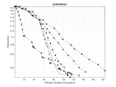
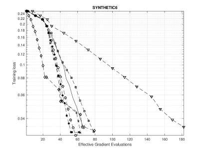
Figure 1: Comparison of ARC-Dynamic (continuous line), ARC-Dynamic C with $C=0.25$ (dashed line with squares), $C=0.5$ (dashed line with circles), $C=0.75$ (dashed line with asterisks), $C=1$ (dashed line with crosses), $C=1.25$ (dashed line with plus symbols), ARC-KL (dashed line with diamonds) and ARC-Sub (dashed line with triangles) against EGE. Each row corresponds to a different synthetic dataset. training loss (left) and testing loss (right) against EGE, logarithmic scale is on the $y$ axis.

Some comments are in order:

• Condition (8.73) in ARC-Sub yields a too high sample size at each iteration. The adaptive strategies ARC-Dynamic and ARC-KL outperform ARC-Sub as in the latter algorithm the cost for computing the Hessians is not compensated by the gain in convergence rate.

• Focusing on the two adaptive strategies ARC-Dynamic and ARC-KL, Table 2 shows that on average the former is less expensive than the latter. Figure 1 shows that ARC-KL is fast in the first stage of the convergence history, becoming progressively slower as the norm of the step starts changing significantly from an iteration to the other (see Figure 3). In fact, the implementation of ARC-KL relies on the assumption that $\|s_{k}\|$ is well approximated by $\|s_{k-1}\|$ and this is not always true. In particular, Figure 3 shows that the norm of the step changes slowly initially while in the remaining iterations it oscillates and successive values differ by some orders of magnitude. This behaviour affects the euclidean norm of the gradient as shown in Figure 2. We observe that such norm, depicted against EGE, oscillates in ARC-KL, while this is not the case in ARC-Dynamic and ARC-Dynamic(C).

• Focusing on our proposed adaptive strategy, Figure 4 shows that ARC-Dynamic uses sets $\mathcal{D}_{k}$ whose cardinality varies adaptively through iterations and it is considerably smaller than $N$ in most iterations. Moreover, the performance of ARC-Dynamic appears to be quite insensitive to the choice of scalar $C$. In fact, computational savings of ARC-Dynamic over ARC-Sub are achieved with various values of $C$, including those reported in Table 1.

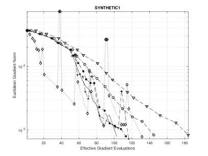
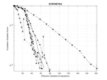
Figure 2: Synthetic datasets, euclidean norm of the gradient against EGE (training set), logarithmic scale is on the $y$ axis. ARC-Dynamic (continuous line), ARC-Dynamic C with $C=0.25$ (dashed line with squares), $C=0.5$ (dashed line with circles), $C=0.75$ (dashed line with asterisks), $C=1$ (dashed line with crosses), $C=1.25$ (dashed line with plus symbols), ARC-KL (dot line with diamonds) and ARC-Sub (dashed line with triangles).

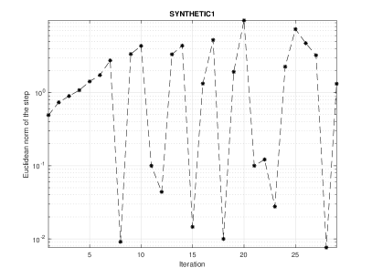
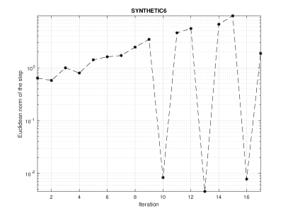
Figure 3: Synthetic datasets, 2-norm of the step against iterations via ARC-KL. Logarithmic scale on the $y$-axis.

Method	Synthetic1	Synthetic2	Synthetic3	Synthetic4	Synthetic6
ARC-Dynamic	98.00%	96.80%	97.10%	97.85%	97.98%
ARC-Dynamic(0.25)	—	—	—	98.09%	98.08%
ARC-Dynamic(0.50)	97.60%	96.40%	96.90%	98.19%	98.23%
ARC-Dynamic(0.75)	98.10%	96.60%	97.20%	98.02%	98.11%
ARC-Dynamic(1.00)	97.20%	96.60%	96.10%	98.15%	97.96%
ARC-Dynamic(1.25)	98.00%	96.60%	96.90%	—	—
ARC-Sub	97.50%	96.60%	97.00%	98.13%	97.87%
ARC-KL	97.80%	96.60%	96.70%	98.13%	97.98%

Table 5: Synthetic datasets. Binary classification rate on the testing set employed by ARC-Dynamic, ARC-Dynamic(C), $C\in\{0.25,0.5,0.75,1,1.25\}$, ARC-KL and ARC-Sub, mean values over $20$ runs.

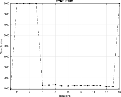
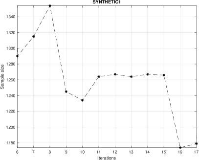
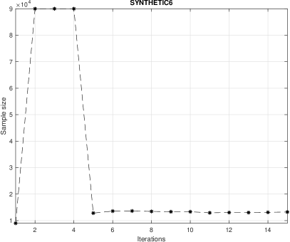
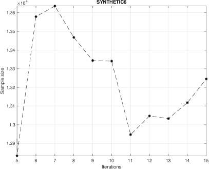
Figure 4: Synthetic datasets. Sample size for Hessian approximations against iterations (left). Portions of figures showing low sample sizes (right).

The synthetic datasets used provide moderately ill-conditioned problems and motivate the use of second order methods. Indeed, second order methods show their strength since all the tested procedures manage to reduce the norm of the gradient and provide a small classification error. This is shown in Table 5 where the average accuracy achieved by methods under comparison is reported. We outline that, the difference between the percentages reported in each column and their mean value ranges from $0.20\%$ (best case) to $0,74\%$ (worst case), with an average of $0,38\%$. Thus, all the ARC variants reach a high accuracy in the testing phase and the preferable one is the variant requiring the lowest number of EGE at termination.

As a final comment, our experiments show that, despite ill-conditioning, an accurate approximation of the Hessian is not required and accuracy dynamically chosen along iterations works well in practice. Adaptive thresholds for the Hessian approximations yield to procedures computationally more convenient than those using constant and tiny thresholds and do not lack ability in solving the problems.

8.3 Real datasets

In this section we present our second set of numerical results, performed on the machine learning datasets using subsampled ARC variants with deterministic suboptimal complexity of $O(\epsilon^{-2})$. More in depth, we compare our adaptive strategy with the version of ARC considered in [35] where, at each iteration, the Hessian is approximated via subsampling on a set with prefixed and small cardinality.

Our adaptive choice of $|{\mathcal{D}_{k}}|$ is implemented by introducing safeguards in (6.65). Whenever $\|s_{k}\|<1$ we choose the cardinality of $\mathcal{D}_{k}$ according the following rule:

$$|\mathcal{D}_{k}|=\max\left\{0.05N,\min\left\{0.1N,\left\lceil\frac{4\rho}{C_{k}}\left(\frac{2\rho}{C_{k}}+\frac{1}{3}\right)\,\log\left(\frac{2n}{\overline{\delta}}\right)\right\rceil\right\}\right\},\quad k\geq 0,$$ (8.75)

with $\rho>0$. Clearly, $|\mathcal{D}_{k}|/N$ varies in the range $[0.05,0.1]$ for all $k\geq 0$, allowing us to compare our adaptive strategy with strategies employing fixed small sample sizes. The scalar $\rho$ is chosen so that $|\mathcal{D}_{k}|=0.1N$ when $C_{k}=\alpha(1-\theta)\epsilon^{2/3}$, i.e., the value of $C_{k}$ corresponding to $\|\nabla f(x_{k})\|=\epsilon^{2/3}$ and $\|s_{k}\|<1$. Whenever $\|s_{k}\|\geq 1$, the scalar $C$ used in (3.21) is fixed so that $|\mathcal{D}_{k}|=0.05N$.

Guidelines for our rule are: sample size $0.05N$ is used when $\|s_{k}\|\geq 1$, larger sample size, up to $0.1N$, is used eventually. Clearly, under this rule the Hessian sample size depends on the ratio $\rho/C_{k}$.

We compare ARC-Dynamic with the above choice of $|\mathcal{D}_{k}|$ against its variant using Hessian approximations obtained by subsampling on a small constant fraction of examples. We will refer to the latter algorithm as ARC-Fix(p) where $p\in(0,1)$ is the prefixed constant fraction of the $N$ examples used for building the Hessian approximations.

In Table 6 we list the datasets used and for sake of completeness, the value of the ratio $\rho/C$ determining the Hessian sample size whenever $\|s_{k}\|\geq 1$ is used. The MNIST dataset is here used for binary classification, labelling even digits with $1$ and odd digits with $0$. In the same table, in the column with header $\epsilon$ we report the used stopping tolerance. All test problems have been solved with $\epsilon=10^{-3}$ except for Cina0 and HTRU2, where the tolerance has been increased to $10^{-2}$, since for lower values of $\epsilon$ we had no longer improvements on the decrease of the training and the testing loss, regardless of the method used. By contrast, Mushroom was solved also using the tighter tolerance $\epsilon=10^{-5}$ as below threshold $\epsilon=10^{-3}$ further reduction in training and testing loss was observed and the percentage of failures in classification on the testing set dropped from 1% to zero. This can be observed in Table 7 where we report the average percentage of testing set data correctly classified. We also underline that, the gap between the percentages reported in each column and their mean value varies from $0\%$ (best case) to $0,89\%$ (worst case), for an average of $0,20\%$. Therefore, the different ARC methods considered achieve a high level of accuracy in the testing phase.

Dataset	Training $N$	$d$	Testing $N_{T}$	$\epsilon$	$\rho/C$
Mushroom [27]	6503	112	1621	$10^{-3}$	2.3241
				$10^{-5}$	2.3241
HTRU2 [27]	10000	8	7898	$10^{-2}$	3.6942
Cina0 [17]	10000	132	6033	$10^{-2}$	2.8671
Gisette [27]	5000	5000	1000	$10^{-3}$	1.6182
MNIST [25]	60000	784	10000	$10^{-3}$	6.3841
A9A [27]	22793	123	9768	$10^{-3}$	4.3922
Ijcnn1 [18]	49990	22	91701	$10^{-3}$	7.5283
Reged0 [18]	400	999	100	$10^{-3}$	0.4443

Table 6: Real datasets. Size of the training set (Training $N$), problem dimension ($d$), size of the testing set (Testing $N_{T}$), tolerance $\epsilon$ for approximate optimality ($\epsilon$) and the ratio $\rho/C$ used for computing sample sizes.

Method	Mushroom		HTRU2	Cina0	Gisette	MNIST	A9A	Ijcnn1	Reged0
	$\epsilon=10^{-3}$	$\epsilon=10^{-5}$
ARC-Dynamic	99.38%	100%	98.20%	91.88%	97.40%	89.92%	84.81%	91.76%	96.00%
ARC-Fix(0.01)	99.07%	100%	98.21%	91.80%	97.60%	89.84%	84.83%	91.95%	96.00%
ARC-Fix(0.05)	98.83%	100%	98.19%	91.84%	97.50%	89.83%	84.76%	91.75%	96.00%
ARC-Fix(0.1)	99.32%	100%	98.20%	91.88%	97.50%	89.77%	84.78%	91.69%	96.00%
ARC-Fix(0.2)	99.20%	100%	98.24%	92.76%	97.30%	89.82%	84.83%	91.70%	96.00%
ARC-Full	98.77%	100%	98.27%	93.10%	97.50%	89.82%	84.87%	91.67%	96.00%

Table 7: Real datasets. Binary classification rate on the testing set employed by ARC-Dynamic, ARC-Fix(p), $p\in\{0.01,0.05,0.1,2\}$ and ARC-Full, mean values over $20$ runs.

In Table 8 we report, for each considered test problem and for each method under comparison, the average number of EGE performed on 20 runs. We compare the performance of ARC-Dynamic with that of ARC-Full and ARC-Fix(p), $p\in\{0.01,0.05,0.1,0.2\}$.

Method	Mushroom		HTRU2	Cina0	Gisette	MNIST	A9A	Ijcnn1	Reged0
	$\epsilon=10^{-3}$	$\epsilon=10^{-5}$
ARC-Dynamic	29.8	75.3	52.2	260.5	195.9	53.4	24.1	26.6	395.6
ARC-Fix(0.01)	41.5	140.1	87.0	405.2	397.3	136.1	37.0	28.4	600.3
ARC-Fix(0.05)	35.5	88.7	86.2	335.6	221.0	101.5	26.2	28.7	503.2
ARC-Fix(0.1)	39.6	92.1	76.1	340.7	231.0	72.8	28.2	31.3	796.3
ARC-Fix(0.2)	38.1	110.7	69.1	453.4	268.8	73.5	34.5	36.1	1353.5
ARC-Full	92.0	264.0	158.0	2300.0	836.0	173.0	87.0	78.0	6932.0

Table 8: Real datasets. Number of EGE employed by ARC-Dynamic, ARC-Fix(p), $p\in\{0.01,0.05,0.1,2\}$ and ARC-Full, mean values over $20$ runs.

Focusing on the strategies employing a prefixed sample size, Table 8 shows that there is not a clear winner, as their performance depend on the specific dataset. However, all of them are clearly preferable to ARC with full Hessian, confirming that uniformly sampling the Hessian on a low number of example is enough and there is no point to compute the full Hessian in these applications. On the other hand, ARC-Dynamic always terminates with the lowest number of EGE and gains over the most effective runs with ARC-Fix(p) range from 11% to 27% in 7 out of 9 test problems and are larger than 20% in the solution of HTRU2, Cina0, MNIST, Reged0. This is confirmed by the performance profile displayed in Figure 5. Denoting by $T$ the set of test problems in Table 6, by $S=\{$ARC-Dynamic, $\{$ARC-Fix(p)$\}$${}_{p\in\{0.01,0.05,0.1,0.2\}}\}$ the set of the considered methods and by $E_{t,s}$ the number of EGE (at termination) to solve the problem $t\in T$ by the solver $s\in S$, the performance profile [22] for each $s\in S$ is defined as the fraction

$$\rho_{s}(\tau)=\frac{1}{|T|}\left|\Set{t\in T:r_{t,s}=\frac{E_{t,s}}{\min\{E_{t,s}:s\in S\}}\leq\tau}\right|,\qquad\tau\geq 1,$$

of problems in $T$ solved by the method $s$ with a performance ratio $r_{t,s}$ within a fraction $\tau$ of the best solver. Comparing the values of $\rho_{s}(1)$, $s\in S$, it can be seen that ARC-Dynamic outperforms the other solvers in the solution of all test problems. As already commented, the performances of the ARC-Fix(p) methods are instead more controversial. More specifically, ARC-Fix(0.01) and ARC-Fix(0.2) seem to be overall less efficient, even if ARC-Fix(0.01) is within a fraction $\tau=1.08$ from the best solver on about $11\%$ of the problems. ARC-Fix(0.05) solved all the problems within $\tau=1.9$ while, within such a value of $\tau$, ARC-Fix(0.1) and ARC-Fix(0.2) solved $89\%$ of the problems and ARC-Fix(0.01) solved $78\%$ of the problems. Moreover, ARC-Fix(0.2) method requires a number of EGE which is within $\tau=3.4$ from the best one to solve all the problems. Finally, in all runs we observed that the decreases of the training and testing loss with ARC-Dynamic is either comparable or faster than with ARC-Fix(p). This features is displayed in Figures 6 where the training and testing loss is plotted versus the number of EGE; representative runs reported concern datasets MNIST and Gisette.

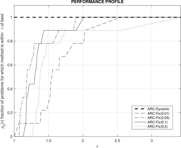
Figure 5: Performance profile (EGE count) on $[1,\leavevmode\nobreak\ 3.4]$ for real datasets.

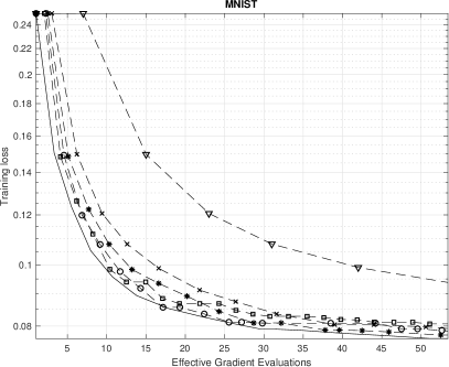
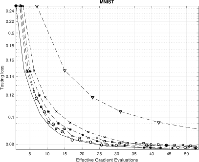
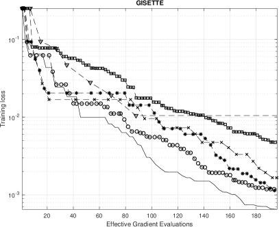
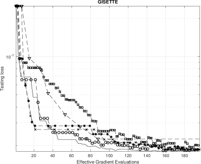
Figure 6: MNIST dataset (top), Gisette dataset (bottom), training loss (left) and testing loss (right) against EGE, logarithmic scale is on the $y$ axis. ARC-Dynamic (continuous line), ARC-Fix(p) with $p=0.2$ (dashed line with crosses), $p=0.1$ (dashed line with asterisks), $p=0.05$ (dashed line with circles), $p=0.01$ (dashed line with squares) and ARC-Full (dashed line with triangles),

9 Conclusions and perspectives

We proposed an ARC algorithm for solving nonconvex optimization problems based on a dynamic rule for building inexact Hessian information. The new algorithm maintains the distinguishing features of ARC framework, i.e., the optimal worst-case iteration bound for first- and second-order critical points. Application to large-scale finite-sum minimization is sketched and analyzed.

In case of sums of strictly convex functions the adaptivity allows to improve complexity results in terms of component Hessian evaluations over approaches that do not employ adaptive rules.

We tested the new algorithm on a large number of problems and compared its performance with the performance of ARC variants with optimal complexity and the performance of ARC variants employing a prefixed small Hessian sample size and showing suboptimal complexity. The former comparison was carried out on synthetic moderately ill-conditioned datasets while the latter comparison was carried out on machine learning datasets from the literature. Numerical results highlight that adaptiveness allows to reduce the overall computational effort and that the performance of the proposed method is quite problem independent while strategies taking a prefixed fraction of samples require a trial and error procedure to set the most efficient sample size.

Convergence properties are analyzed both under deterministic and probabilistic conditions, in the latter case properties of the deterministic algorithm are preserved in high probability. However, this analysis does not give indication on the properties of the method when the adaptive accuracy requirement is not satisfied. A stochastic analysis, in the spirit of [16], would be of interest and it is the topic of future research. Moreover, we here assume that the objective function and the gradient are exact. Extensions of this approach to the case where both function and gradient are evaluated with adaptive accuracy is desirable as well as the employment of variance reduction techniques.

10 Acknowledgements

The authors wish to thank Raghu Bollapragada for gently providing the synthetic datasets and the referees for their insightful comments.

References

- [1] J. Barzilai, J. M. Borwein (1988), Two-Point Step Size Gradient Methods, IMA Journal of Numerical Analysis, 8, pp. 14–148.
- [2] S. Bellavia, G. Gurioli, B. Morini, Ph. L. Toint (2019) Adaptive Regularization Algorithms with Inexact Evaluations for Nonconvex Optimization. arXiv:1811.03831.
- [3] S. Bellavia, N. Krejic, N. Krklec Jerinkic (2018) Subsampled Inexact Newton methods for minimizing large sums of convex functions. http://www.optimization-online.org/DB_HTML/2018/01/6432.html.
- [4] S. Bellavia, N. Krejic, B. Morini, Inexact restoration with subsampled trust-region methods for finite-sum minimization. arXiv:1902.01710.
- [5] A.S. Berahas, R. Bollapragada, J. Nocedal (2017) An investigation of Newton-sketch and subsampled Newton methods. arXiv:1705.06211.
- [6] T. Bianconcini, G. Liuzzi, B. Morini, M. Sciandrone (2015) On the use of iterative methods in cubic regularization for unconstrained optimization. Comp. Optim. Appl., 60, 35–57.
- [7] E.G. Birgin, J.L. Gardenghi, J.M. Martínez, S.A. Santos and Ph.L. Toint (2017) Worst-case evaluation complexity for unconstrained nonlinear optimization using high-order regularized models. Math. Progr., Ser. A 163, 359-368.
- [8] L. Bottou, F.E. Curtis, J. Nocedal (2018) Optimization Methods for Large-Scale Machine Learning, SIAM Review, 60, 223-311.
- [9] R.H. Byrd, G.M. Chin, W. Neveitt, J. Nocedal (2018) On the Use of Stochastic Hessian Information in Optimization Methods for Machine Learning. SIAM J. Optim., 21, 977–995.
- [10] Y. Carmon, J.C. Duchi (2016) Gradient descent efficiently finds the cubic-regularized non-convex Newton step, arXiv:1612.00547.
- [11] C. Cartis, N.I.M. Gould and Ph.L. Toint (2010) On the complexity of steepest descent, Newton’s and regularized Newton’s method for nonconvex unconstrained optimization. SIAM J. Optim., 20, 2833–2852.
- [12] C. Cartis, N.I.M. Gould, Ph.L. Toint (2011) Adaptive cubic regularisation methods for unconstrained optimization. Part I: motivation, convergence and numerical results. Math. Progr., Ser. A, 127, 245-295.
- [13] C. Cartis, N.I.M. Gould, Ph.L. Toint (2011) Adaptive cubic overestimation methods for unconstrained optimization. Part II: worst-case function and derivative-evaluation complexity. Math. Progr., Ser. A, 130, 295–319
- [14] C. Cartis, N.I.M. Gould, Ph.L. Toint (2012) Complexity bounds for second-order optimality in unconstrained optimization. J. Complex., 28, 93–108.
- [15] C. Cartis, N.I.M. Gould and Ph.L. Toint (2012) An adaptive cubic regularisation algorithm for nonconvex optimization with convex constraints and its function-evaluation complexity. IMA J. Numer. Anal., 32, 1662–1695.
- [16] C. Cartis, K. Scheinberg (2018) Global convergence rate analysis of unconstrained optimization methods based on probabilistic models Math. Progr., Ser. A, 169, 337–375.
- [17] (2008) Causality workbench team, A marketing dataset, http://www.causality.inf.ethz.ch/data/CINA.html.
- [18] C.C. Chang, C.J. Lin (2011) LIBSVM : a library for support vector machines. ACM Transactions on Intelligent Systems and Technology, 2(3):27 http://www.csie.ntu.edu.tw/ cjlin/libsvm.
- [19] X. Chen, B. Jiang, T. Lin, S. Zhang (2018) On Adaptive Cubic Regularized Newton’s Methods for Convex Optimization via Random Sampling. arXiv:1802.05426.
- [20] A.R. Conn, N.I.M. Gould, and Ph.L. Toint. (2000)Trust-Region Methods. No. 1 in the ’MPS–SIAM series on optimization’, Philadelphia, USA: SIAM.
- [21] J.E. Dennis, J.J. Moré (1974) A characterization of superlinear convergence and its application to quasi-Newton methods. Math. Comput., 28, 549–560.
- [22] E. D. Dolan, J. J. Moré (2002). Benchmarking optimization software with performance profiles. Math. Program., 91(2), 201–213.
- [23] A. Griewank (1981) The modification of Newton’s method for unconstrained optimization by bounding cubic terms. Technical Report NA/12, Department of Applied Mathematics and Theoretical Physics, University of Cambridge, United Kingdom
- [24] J.M. Kohler, A. Lucchi (2017) Subsampled cubic regularization for non-convex optimization 34th International Conference on Machine Learning, ICML 2017. 4, 2988-3011.
- [25] Y. LeCun, L. Bottou, Y. Bengio, P. Haffner (1998) Gradient-based learning applied to document recognition. Proceedings of the IEEE, 86 2278-2324. MNIST database available at http://yann.lecun.com/exdb/mnist/.
- [26] J.D. Lee, M. Simchowitz, M.I. Jordan, B. Recht (2016) Gradient Descent Only Converges to Minimizers. JMRL: Workshop and Conference Proceedings, 49, 1–12.
- [27] M. Lichman(2013) UCI machine learning repository, https://archive.ics.uci.edu/ml/index.php.
- [28] J.J. Moré, D.C. Sorensen. (1983) Computing a trust region step. SIAM J. Sci. Statist. Comput., 4, 553–572.
- [29] I. Mukherjee, K. Canini, R. Frongillo, Y. Singer (2013). Joint European Conference on Machine Learning and Knowledge Discovery in Databases, Springer Berlin Heidelberg, 17–32.
- [30] Y. Nesterov and B.T. Polyak (2006) Cubic regularization of Newton’s method and its global performance. Math. Progr., Ser. A, 108, 177–205.
- [31] M. Pilanci and M. J. Wainwright. (2017) Newton sketch: A near linear-time optimization algorithm with linear-quadratic convergence. SIAM J. Optim., 27, 205–245.
- [32] F. Roosta-Khorasani, M.W. Mahoney. (2019) Sub-Sampled Newton Methods, Math. Prog, 174, 293–326.
- [33] M. Weiser, P. Deuflhard, B. Erdmann (2007) Affine conjugate adaptive Newton methods for nonlinear elastomechanics. Optim. Methods Softw., 22, 413–431.
- [34] P. Xu, F. Roosta-Khorasani, M.W. Mahoney (2019) Newton-Type Methods for Non-Convex Optimization Under Inexact Hessian Information, Math. Prog, https://doi.org/10.1007/s10107-019-01405-z.
- [35] P. Xu, F. Roosta-Khorasani, M.W. Mahoney (2017) Second-order optimization for non-convex machine learning: an empirical study. arXiv:1708.07827.
- [36] Z. Yao, P. Xu, F.Roosta-Khorasani, M.W. Mahoney (2018) Inexact non-convex Newton-type methods. arXiv:1802.06925.
- [37] D. Zhou, P. Xu, Q. Gu, (2019) Stochastic Variance-Reduced Cubic Regularization Methods. Journal of Machine Learning Research, 20, pp.1–47.