Improved Decision Rule Approximations for Multi-Stage Robust Optimization via Copositive Programming

Guanglin Xu       Grani A. Hanasusanto Institute for Mathematics and its Applications, University of Minnesota, Minneapolis, MN, 55455, USA. Email: gxu@umn.edu.Graduate Program in Operations Research and Industrial Engineering, The University of Texas at Austin, Austin, TX, 78712-1591, USA. Email: grani.hanasusanto@utexas.edu.
Abstract

We study decision rule approximations for generic multi-stage robust linear optimization problems. We examine linear decision rules for the case when the objective coefficients, the recourse matrices, and the right-hand sides are uncertain, and examine quadratic decision rules for the case when only the right-hand sides are uncertain. The resulting optimization problems are NP-hard but amenable to copositive programming reformulations that give rise to tight, tractable semidefinite programming solution approaches. We further enhance these approximations through new piecewise decision rule schemes. Finally, we prove that our proposed approximations are tighter than the state-of-the-art schemes and demonstrate their superiority through numerical experiments.

Keywords: Multi-stage robust optimization; decision rules; piecewise decision rules; conservative approximation; copositive programming; semidefinite programming

1 Introduction

Decision-making under uncertainty arises in a wide spectrum of applications in operations management, engineering, finance, and process control. A prominent modeling approach for decision-making under uncertainty is robust optimization (RO), whereby one seeks for a decision that hedges against the worst-case realization of uncertain parameters; see [8, 14, 15]. RO paradigm is appealing because it leads to computationally tractable solution schemes for many static decision-making problems under uncertainty. However, real-life problems are often dynamic in nature, where the uncertain parameters are revealed sequentially and the decisions must be adapted to the current realizations. The adaptive decisions are fundamentally infinite-dimensional as they constitute mappings from the space of uncertain parameters to the space of actions. This setting gives rise to the multi-stage robust optimization (MSRO) problems which in general are computationally challenging to solve. Only in a few cases and under very stringent conditions are the problems efficiently solvable; see for instance [13, 21, 50]. Consequently, the design of solution schemes for MSRO necessitates to reconcile the conflicting objectives of optimality and scalability.

Conservative approximations for MSRO can be derived in linear decision rules, where we restrict the adaptive decisions to affine functions in the uncertain parameters. Popularized by Ben-Tal et al. [11], linear decision rules have found successful applications in various areas of decision-making problems under uncertainty [5, 10, 32, 34, 35, 49, 65] as they are simple yet reasonable to implement in practice. Moreover, linear decision rules are optimal for some instances of MSRO [20, 55], linear quadratic optimal control [2], and robust vehicle routing [49] problems. The resulting optimization problems, however, are tractable only under the restrictive setting of fixed recourse, i.e., when the adaptive decisions are not multiplied with the uncertain parameters in the problem’s formulation. Many decision-making problems under uncertainty such as portfolio optimization [12, 37, 65], energy systems operation planning [46, 60], inventory planning [19], etc. do not satisfy the fixed recourse assumption. For these problem instances, the linear decision rule approximation is NP-hard already in a two-stage setting [11, 50].

The basic linear decision rules have been extended to truncated linear [66], segregated linear [35, 36, 47], and piecewise linear [9, 45] functions in the uncertain parameters. If the MSRO problem has fixed recourse then one can formally prove that the optimal adaptive decisions are piecewise linear [7], which justifies the use of these enhanced approximations. Unfortunately, optimizing for the best piecewise linear decision rule entails solving globally a non-convex optimization problem which is inherently difficult [9, 18]. If in addition some basic descriptions about the piecewise linear structure are prescribed, then one can derive tractable linear programming approximations for problem instances with fixed recourse by Georghiou et al. [45]. Their piecewise linear decision rule scheme is a generalization of the aforementioned methods, including the truncated linear decision rule [66] and the segregated linear decision rule [35, 36, 47].

If tighter approximation is desired or when the problem has non-fixed recourse, then one can in principle develop a hierarchy of increasingly tight semidefinite approximations using polynomial decision rules [23]. While optimizing for the best polynomial decision rule of fixed degree is difficult, tractable conservative approximations can be obtained by employing the Lasserre hierarchy [58, 63]. Such approximations are attractive because they do not require prior structural knowledge about the optimal adaptive decisions. However, the resulting semidefinite programs scale poorly with the degree of the polynomial decision rules. A decent tradeoff between suboptimality and scalability is attained in quadratic decision rules, where one merely optimizes over polynomial functions of degree $2$. Their semidefinite approximations, based on the well-known approximate S-lemma [8], have been applied successfully to instances of inventory planning [23, 53] and electricity capacity expansion [6] problems. A posteriori lower bounds to the MSRO problem can be derived by applying decision rules to the problem’s dual formulation [6, 45, 57]. Alternative schemes that similarly provide aggressive bounds for MSRO are proposed in [51] and [16]. All the methods mentioned above can be applied to different paradigms in optimization under uncertainty, such as stochastic programming, robust optimization, and distributionally robust optimization. Our paper focuses on the robust optimization setting because it requires minimal assumptions about the uncertainty, which allows us to present the main idea cleanly. If distributional information is available, then the proposed method can be directly applied to the other settings in a relatively straightforward fashion.

Global optimization approaches have also been designed to derive exact solutions of MSRO problems. In the two-stage robust optimization setting, these methods include Benders’ decomposition [24, 39], column and constraint generation [68], extreme point enumeration combined with decision rules [44], and Fourier-Motzkin elimination [69]. The Benders’ decomposition scheme has been extended to the multi-stage setting for MSRO problems where the uncertain parameters exhibit a stagewise rectangular structure [43]. The papers [17] and [64] develop adaptive uncertainty set partitioning schemes that generate a sequence of increasingly accurate conservative approximations for MSRO. Global optimization scheme has also been conceived through the lens of conic reformulations. Hanasusanto and Kuhn [52] and Xu and Burer [67] propose independently equivalent copositive programming reformulations for two-stage robust optimization problems and develop conservative semidefinite approximations for the reformulations.

Using copositive programming techniques, this paper takes a first step towards addressing a generic linear MSRO problem where the objective coefficients, the recourse matrix, and the right-hand sides are uncertain. A copositive program is a convex program that optimizes a linear function over the cone of copositive matrices subject to linear constraints [26, 29, 40]. Bomze et al. [27] are the first to reformulate an NP-hard problem, namely the standard quadratic problem, to an equivalent copositive program. The seminal work of Burer [28] shows that a generic quadratic program can be reformulated to an equivalent copositive program. In another work, Burer and Dong [31] establish the equivalence between a non-convex quadratically constrained quadratic program (QCQP) and a generalized copositive program under certain conditions. We refer the reader to [31, 33, 56, 61, 62] for more works on using copositive techniques to reformulate non-convex quadratic programs arising in different applications.

Our key contribution is to utilize copositive programming techniques to develop stronger decision rule approximations for generic MSRO problems. In the generic settings, the direct use of decision rules leads to computationally intractable semi-infinite programs, with finitely many decision variables but infinitely many constraints. The standard dualization procedure in robust optimization does not apply because these constraints involve non-convex QCQPs. We leverage the copositive reformulation techniques to convexify the QCQPs, which enables the dualization of the constraints to arrive at finite-dimensional convex optimization problems. The copositive techniques further allow us to handle complex uncertainty sets (e.g., integrating complementary constraints), which lead to exact convex reformulations for a class of piecewise decision rule approximations. All these new reformulations enjoy tractable semidefinite approximations that are provably superior to the state-of-the-art schemes. We summarize the contributions of the paper as follows.

  1. 1.

    For the generic MSRO problems we derive new copositive programming reformulations in view of the popular linear decision rules. For MSRO problems with fixed recourse we derive new copositive programming reformulations in view of the more powerful quadratic decision rules. The exactness results are general: They hold for MSRO problems without relatively complete recourse, and under very minimal assumption about the compactness of the uncertainty set, without requiring it to exhibit stage-wise rectangularity.

  2. 2.

    The emerging copositive programs are amenable to a hierarchy of increasingly tight conservative semidefinite programming approximations. We formulate the simplest of these approximations and prove that it is tighter than the state-of-the-art scheme by Ben-Tal et al. [11], and also the polynomial decision rule scheme by Bertsimas et al. [23] when the degree of the polynomial is set to the degree of our decision rules (degree $1$ for problems with non-fixed recourse and degree $2$ for problems with fixed recourse). We demonstrate empirically that our proposed approximation is competitive to polynomial decision rules of higher degrees while displaying more favorable scalability.

  3. 3.

    We propose piecewise linear decision rules for MSRO problems with non-fixed recourse and piecewise quadratic decision rules for MSRO problems with fixed recourse. To our best knowledge, these decision rules are new for their respective problem classes. By leveraging recent techniques in copositive programming, we derive equivalent copositive programs for the piecewise decision rule approximations. For MSRO problems with fixed recourse, we show that the state-of-the-art scheme by Georghiou et al. [45] can be futile even on trivial two-stage problem instances, while our semidefinite approximation produces high-quality solutions. We formally prove that our proposed approximation is indeed tighter than that of [45], and further identify the simplest set of semidefinite constraints that retains the outperformance while maintaining scalability.

The remainder of the paper is organized as follows. We derive the copositive programming reformulations for two-stage robust optimization problems in Section 2. In Section 3, we develop the conservative semidefinite programming approximations. We extend all results to the multi-stage setting in Section 4 and present the numerical results in Section 5.

1.1 Notation and terminology

For any $M\in\mathbb{N}$, we define $[M]$ as the set of running indices $\{1,\ldots,M\}$. We let $[M]\backslash\{1\}$ be the set of running indices $\{2,\ldots,M\}$. We denote by $\mathbf{e}$ the vector of all ones and by $\mathbf{e}_{i}$ the $i$-th standard basis vector. For notational convenience, we use both $v_{i}$ and $[\boldsymbol{v}]_{i}$ to denote the $i$-th component of the vector $\boldsymbol{v}$. The $p$-norm of a vector $\boldsymbol{v}\in{\mathbb{R}}^{N}$ is defined as $\|\boldsymbol{v}\|_{p}$. We will drop the subscript for the Euclidean norm, i.e., $\|\boldsymbol{v}\|:=\|\boldsymbol{v}\|_{2}$. For $\boldsymbol{a}\in{\mathbb{R}}^{N}$ and $\boldsymbol{b}\in{\mathbb{R}}^{N}$, the Hadamard product of $\boldsymbol{a}$ and $\boldsymbol{b}$ is denoted by $\boldsymbol{a}\circ\boldsymbol{b}:=(a_{1}b_{1},\ldots,a_{N}b_{N})^{\top}$. The trace of a square matrix $\boldsymbol{X}$ is denoted as $\text{trace}(\boldsymbol{X})$. We use $[\boldsymbol{A}]_{ij}$ to denote the entry in the $i$-th row and the $j$-th column of the matrix $\boldsymbol{A}$. We define $\operatorname{diag}(\boldsymbol{X})$ as the vector comprising the diagonal entries of $\boldsymbol{X}$, and $\operatorname{Diag}(\boldsymbol{v})$ as the diagonal matrix with the vector $\boldsymbol{v}$ along its main diagonal. We use $\boldsymbol{X}\geq\boldsymbol{0}$ to denote that $\boldsymbol{X}$ is a component-wise nonnegative matrix. For any matrix $\boldsymbol{A}\in{\mathbb{R}}^{M\times N}$, the inclusion $\text{Rows}(\boldsymbol{A})\in{\mathcal{K}}$ indicates that the column vectors corresponding to the rows of $\boldsymbol{A}$ are members of ${\mathcal{K}}$. We denote by ${\mathscr{F}}_{K+1,\,N}$ the space of all measurable mappings ${\mathscr{\boldsymbol{y}}}(\cdot)$ from ${\mathbb{R}}^{K+1}$ to ${\mathbb{R}}^{N}$.

For any closed and convex cone ${\cal K}$, we denote its dual cone as ${\cal K}^{*}$. We define by ${\mathcal{SOC}}\subseteq{\mathbb{R}}^{K+1}$ the standard second-order cone, i.e., $\boldsymbol{v}\in{\mathcal{SOC}}\Longleftrightarrow\|(v_{1},\ldots,v_{K})^{\top}\|\leq v_{K+1}$. We denote the space of symmetric matrices in $\mathbb{R}^{N\times N}$ as ${\mathcal{S}}^{N}$. For any $\boldsymbol{X}\in{\mathcal{S}}^{N}$, we set $\boldsymbol{X}\succeq\boldsymbol{0}$ to denote that $\boldsymbol{X}$ is positive semidefinite. For convenience, we call the cone of positive semidefinite matrices as the semidefinite cone and the cone of symmetric nonnegative matrices as the the nonnegative cone. The copositive cone is defined as $\mathcal{COP}({\mathbb{R}}_{+}^{N}):=\{\boldsymbol{M}\in{\mathcal{S}}^{N}:{\boldsymbol{x}}^{\top}\boldsymbol{M}{\boldsymbol{x}}\geq 0\ \forall{\boldsymbol{x}}\in{\mathbb{R}}_{+}^{N}\}$. Its dual cone, the completely positive cone, is defined as $\mathcal{CP}({\mathbb{R}}_{+}^{N}):=\{\boldsymbol{X}\in{\mathcal{S}}^{N}:\boldsymbol{X}=\textstyle{\sum_{i}}{\boldsymbol{x}}^{i}({\boldsymbol{x}}^{i})^{\top},\ {\boldsymbol{x}}^{i}\in{\mathbb{R}}_{+}^{N}\}$, where the summation over $i$ is finite but its cardinality is unspecified. For a general closed and convex cone ${\cal K}\subseteq{\mathbb{R}}^{N}$, we define the generalized copositive cone as $\mathcal{COP}({\cal K})$ and the generalized completely positive cone as $\mathcal{CP}({\cal K})$, respectively, in analogy with $\mathcal{COP}({\mathbb{R}}_{+}^{N})$ and $\mathcal{CP}({\mathbb{R}}_{+}^{N})$. Note that $\mathcal{COP}({\cal K})$ and $\mathcal{CP}({\cal K})$ are dual cones to each other. The term copositive programming refers to linear optimization over $\mathcal{COP}({\cal K})$ or, via duality, linear optimization over $\mathcal{CP}({\cal K})$. To distinguish from the standard case where ${\cal K}={\mathbb{R}}_{+}^{N}$, they are sometimes called generalized copositive programming or set-semidefinite optimization [31, 41]. In this paper, we work with generalized copositive programming, although we use the shorter phrase for simplicity.

2 Copositive reformulations for two-stage decision rule problems

In this section, we first state the generic setting of a two-stage robust optimization problem. We then consider various decision rules for the two-stage problem and propose copositive programming reformulations for the decision rule problems.

2.1 Two-stage robust optimization problem

We study adaptive linear optimization problems of the following general structure. A decision maker first takes a here-and-now decision $\boldsymbol{x}\in{\mathcal{X}}$, which incurs an immediate linear cost $\boldsymbol{c}^{\top}\boldsymbol{x}$. Nature then reacts with a worst-case parameter realization $\boldsymbol{u}\in{\mathcal{U}}$. In response, the decision maker takes a recourse action $\boldsymbol{y}(\boldsymbol{u})\in{\mathbb{R}}^{N}$, which incurs a second-stage linear cost ${\boldsymbol{d}}({\boldsymbol{u}})^{\top}{\mathscr{\boldsymbol{y}}}({\boldsymbol{u}})$. In this game against nature, the decision maker endeavors to optimally select a feasible solution $(\boldsymbol{x},{\mathscr{\boldsymbol{y}}}(\cdot))$ that minimizes the total cost ${\boldsymbol{c}}^{\top}{\boldsymbol{x}}+\sup_{{\boldsymbol{u}}\in{\mathcal{U}}}{\boldsymbol{d}}({\boldsymbol{u}})^{\top}{\mathscr{\boldsymbol{y}}}({\boldsymbol{u}})$. We note that the second-stage decision vector constitutes a mapping ${\mathscr{\boldsymbol{y}}}:{\mathcal{U}}\rightarrow{\mathbb{R}}^{N}$ and is thus infinite dimensional.

The emerging sequential decision problem can be formulated as a two-stage robust optimization problem given by

$$\begin{array}[]{rcl}Z=&\inf&{\boldsymbol{c}}^{\top}{\boldsymbol{x}}+\sup\limits_{{\boldsymbol{u}}\in{\mathcal{U}}}{\boldsymbol{d}}({\boldsymbol{u}})^{\top}{\mathscr{\boldsymbol{y}}}({\boldsymbol{u}})\\ &\operatorname{s.t.}&{\boldsymbol{\mathcal{A}}}({\boldsymbol{u}}){\boldsymbol{x}}+{\boldsymbol{\mathcal{B}}}({\boldsymbol{u}}){\mathscr{\boldsymbol{y}}}({\boldsymbol{u}})\geq{\boldsymbol{h}}({\boldsymbol{u}})\ \ \ \forall\,{\boldsymbol{u}}\in{\mathcal{U}}\\ &&{\boldsymbol{x}}\in{\mathcal{X}},\ {\mathscr{\boldsymbol{y}}}\in{\mathscr{F}}_{K+1,\,N}.\end{array}$$ (1)

Here, the feasible set of the first-stage decision ${\boldsymbol{x}}$ is captured by a generic set ${\mathcal{X}}\subseteq{\mathbb{R}}^{M}$, while that of the second-stage decision $\boldsymbol{y}(\boldsymbol{u})$ is defined through a linear constraint system ${\boldsymbol{\mathcal{A}}}({\boldsymbol{u}}){\boldsymbol{x}}+{\boldsymbol{\mathcal{B}}}({\boldsymbol{u}}){\mathscr{\boldsymbol{y}}}({\boldsymbol{u}})\geq{\boldsymbol{h}}({\boldsymbol{u}})$. The uncertain parameter vector ${\boldsymbol{u}}$ is assumed to belong to a prescribed uncertainty set ${\mathcal{U}}$, which we model as the intersection of a slice of a closed and convex cone ${\mathcal{K}}\subseteq{\mathbb{R}}^{K}\times{\mathbb{R}}_{+}$, and the level sets of $I$ quadratic functions. Specifically, we set

$${\mathcal{U}}:=\left\{{\boldsymbol{u}}\in{\mathcal{K}}:\begin{array}[]{l}\mathbf{e}_{K+1}^{\top}{\boldsymbol{u}}=1\\[5.69054pt] {\boldsymbol{u}}^{\top}\boldsymbol{\widehat{C}}_{i}{\boldsymbol{u}}=0\ \ \ \forall\,i\in[I]\end{array}\right\},$$ (2)

where $\boldsymbol{\widehat{C}}_{i}\in{\mathcal{S}}^{K+1}$ for all $i\in[I]$. The problem parameters ${\boldsymbol{\mathcal{A}}}({\boldsymbol{u}})\in{\mathbb{R}}^{J\times M}$, ${\boldsymbol{\mathcal{B}}}({\boldsymbol{u}})\in{\mathbb{R}}^{J\times N}$, ${\boldsymbol{d}}({\boldsymbol{u}})\in{\mathbb{R}}^{N}$ and ${\boldsymbol{h}}({\boldsymbol{u}})\in{\mathbb{R}}^{J}$ in (1) are assumed to be linear in ${\boldsymbol{u}}$, given by

$$\begin{array}[]{l}{\boldsymbol{\mathcal{A}}}({\boldsymbol{u}})=\sum\limits_{k=1}^{K+1}u_{k}\,\boldsymbol{\widehat{A}}_{k},\ \ \ {\boldsymbol{\mathcal{B}}}({\boldsymbol{u}})=\sum\limits_{k=1}^{K+1}u_{k}\,\boldsymbol{\widehat{B}}_{k},\ \ \ {\boldsymbol{d}}({\boldsymbol{u}})=\boldsymbol{\widehat{D}}{\boldsymbol{u}},\ \ \ {\boldsymbol{h}}({\boldsymbol{u}})=\boldsymbol{\widehat{H}}{\boldsymbol{u}},\end{array}$$

where $\boldsymbol{\widehat{A}}_{k}\in{\mathbb{R}}^{J\times M}$, $\boldsymbol{\widehat{B}}_{k}\in{\mathbb{R}}^{J\times N}$, $\boldsymbol{\widehat{D}}:=(\boldsymbol{\widehat{d}}_{1},\ldots,\boldsymbol{\widehat{d}}_{N})^{\top}\in{\mathbb{R}}^{N\times(K+1)}$, and $\boldsymbol{\widehat{H}}:=(\boldsymbol{\widehat{h}}_{1},\ldots,\boldsymbol{\widehat{h}}_{J})^{\top}\in{\mathbb{R}}^{J\times(K+1)}$ are deterministic data. The nonrestrictive assumption that $u_{K+1}=1$ in (2) will simplify notation as it allows us to represent affine functions in the primitive uncertain parameters $(u_{1},\ldots,u_{K})^{\top}$ in a compact way as linear functions of $\boldsymbol{u}$, e.g., the problem parameters ${\boldsymbol{\mathcal{A}}}({\boldsymbol{u}})$, ${\boldsymbol{\mathcal{B}}}({\boldsymbol{u}})$, ${\boldsymbol{d}}({\boldsymbol{u}})$, and ${\boldsymbol{h}}({\boldsymbol{u}})$, and the linear decision rule $\boldsymbol{Y}{\boldsymbol{u}}$ (Section 2.2); and as it also allows us to represent quadratic functions in the primitive uncertain parameters in a homogenized manner, e.g., the quadratic decision rule ${\boldsymbol{u}}^{\top}\boldsymbol{Q}{\boldsymbol{u}}$ (Section 2.2).

The cone ${\mathcal{K}}$ in the description of ${\mathcal{U}}$ has a generic form and can model many common uncertainty sets in the literature. We highlight three pertinent examples as follows.

Example 1 (Polytope).

If the uncertainty set of the primitive vector $(u_{1},\dots,u_{K})^{\top}$ is given by a polytope $\{\boldsymbol{\xi}\in{\mathbb{R}}^{K}:\boldsymbol{P}\boldsymbol{\xi}\geq\boldsymbol{q}\}$, then the corresponding cone is defined as

$${\mathcal{K}}:=\left\{(\boldsymbol{\xi},\tau)\in{\mathbb{R}}^{K}\times{\mathbb{R}}_{+}:\boldsymbol{P}\boldsymbol{\xi}\geq\boldsymbol{q}\tau\right\}.$$
Example 2 (Polytope and 2-Norm Ball).

If the uncertainty set of the primitive vector is given by the intersection of a polytope and a transformed $2$-norm ball: $\{\boldsymbol{\xi}\in{\mathbb{R}}^{K}:\boldsymbol{P}\boldsymbol{\xi}\geq\boldsymbol{q},\;\|\boldsymbol{R}\boldsymbol{\xi}-\boldsymbol{s}\|_{2}\leq t\}$, then the corresponding cone is defined as

$${\mathcal{K}}:=\left\{(\boldsymbol{\xi},\tau)\in{\mathbb{R}}^{K}\times{\mathbb{R}}_{+}:\boldsymbol{P}\boldsymbol{\xi}\geq\boldsymbol{q}\tau,\,\|\boldsymbol{R}\boldsymbol{\xi}-\boldsymbol{s}\tau\|\leq t\tau\right\}.$$
Example 3 (Ellipsoids).

Consider the setting where the uncertainty set of the primitive vector is described by an intersection of $L$ ellipsoids: $\{\boldsymbol{\xi}\in{\mathbb{R}}^{K}:\boldsymbol{\xi}^{\top}\boldsymbol{F}_{\ell}\boldsymbol{\xi}+2\boldsymbol{g}_{\ell}^{\top}\boldsymbol{\xi}\leq h_{\ell},\;\forall\ell\in[L]\}$. Here, $\boldsymbol{F}_{\ell}\in{\mathcal{S}}^{K}$, $\boldsymbol{F}_{\ell}\succeq\boldsymbol{0}$, $\boldsymbol{g}_{\ell}\in{\mathbb{R}}^{K}$, and $h_{\ell}\in{\mathbb{R}}$ for all $\ell\in[L]$. Since $\boldsymbol{F}_{\ell}$ is positive semidefinite, we have $\boldsymbol{F}_{\ell}=\boldsymbol{P}_{\ell}^{\top}\boldsymbol{P}_{\ell}$ for some matrix $\boldsymbol{P}_{\ell}\in{\mathbb{R}}^{I_{\ell}\times K}$ whose rank is $I_{\ell}$. In [1], it is shown that

$$\boldsymbol{\xi}^{\top}\boldsymbol{F}_{\ell}\boldsymbol{\xi}+2\boldsymbol{g}_{\ell}^{\top}\boldsymbol{\xi}\leq h_{\ell}\ \ \Longleftrightarrow\ \ \begin{pmatrix}\boldsymbol{P}_{\ell}\boldsymbol{\xi}\\ \frac{1}{2}(1-h_{\ell})+\boldsymbol{g}_{\ell}^{\top}\boldsymbol{\xi}\\ \frac{1}{2}(1+h_{\ell})-\boldsymbol{g}_{\ell}^{\top}\boldsymbol{\xi}\end{pmatrix}\in\mathcal{SOC}(I_{\ell}+2),$$

where $\mathcal{SOC}(I_{\ell}+2)$ denotes the second-order cone of dimension $I_{\ell}+2$. In this case, the corresponding cone is given by

$${\mathcal{K}}:=\left\{(\boldsymbol{\xi},\tau)\in{\mathbb{R}}^{K}\times{\mathbb{R}}_{+}:\begin{pmatrix}\boldsymbol{P}_{\ell}\boldsymbol{\xi}\\ \frac{1}{2}(1-h_{\ell})\tau+\boldsymbol{g}_{\ell}^{\top}\boldsymbol{\xi}\\ \frac{1}{2}(1+h_{\ell})\tau-\boldsymbol{g}_{\ell}^{\top}\boldsymbol{\xi}\end{pmatrix}\in\mathcal{SOC}(I_{\ell}+2)\ \ \forall\,\ell\in[L]\right\}.$$

In the following, to simplify our exposition, we define the convex set

$${{\mathcal{U}^{0}}}:=\left\{{\boldsymbol{u}}\in{\mathcal{K}}:\mathbf{e}_{K+1}^{\top}{\boldsymbol{u}}=1\right\},$$ (3)

which corresponds to the uncertainty set $\mathcal{U}$ in the absence of the non-convex constraints ${\boldsymbol{u}}^{\top}\boldsymbol{\widehat{C}}_{i}{\boldsymbol{u}}=0$, $i\in[I]$. We further assume that the uncertainty set satisfies the following regularity conditions.

Assumption ​​ 1.

The set ${{\mathcal{U}^{0}}}$ defined in (3) is nonempty and compact.

Assumption ​​ 2.

The minimum value of the quadratic function ${\boldsymbol{u}}^{\top}\boldsymbol{\widehat{C}}_{i}{\boldsymbol{u}}$ over the set ${{\mathcal{U}^{0}}}$ is 0 for all $i\in[I]$, i.e., $0=\min_{{\boldsymbol{u}}\,\in\,{{\mathcal{U}^{0}}}}{\boldsymbol{u}}^{\top}\boldsymbol{\widehat{C}}_{i}{\boldsymbol{u}}$, $i\in[I]$.

The quadratic constraints in the description of ${\mathcal{U}}$ are motivated by both practical and modeling requirements. Numerous applications in robust optimization, including inventory planning and project crashing problems, involve binary uncertain parameters; see [48]. In this case, we can incorporate binary variables in ${\mathcal{U}}$ via quadratic constraints of the form in (2). Specifically, we have that $u_{k}\in\{0,1\}$ is equivalent to $u_{k}^{2}=u_{k}$. If the relation $0\leq u_{k}\leq 1$ is implied by ${\mathcal{U}^{0}}$ (note that we can explicitly introduce these constraints into ${\mathcal{U}^{0}}$ if necessary), then we have $0=\min_{{\boldsymbol{u}}\in{\mathcal{U}^{0}}}\left\{-u_{k}^{2}+u_{k}\right\}$, which shows that the quadratic constraint $-u_{k}^{2}+u_{k}=0$ satisfies the condition in Assumption 2. Furthermore, these constraints will be crucial for deriving our improved decision rules as they enable us to model complementary constraints, e.g., $u_{k}u_{k^{\prime}}=0$; see Section 2.4 for detail. If ${\mathcal{U}^{0}}$ implies that both $u_{k}$ and $u_{k^{\prime}}$ are nonnegative and bounded, then we have $0=\min_{{\boldsymbol{u}}\in{\mathcal{U}^{0}}}\left\{u_{k}u_{k^{\prime}}\right\}$. Thus, the quadratic constraint $u_{k}u_{k^{\prime}}=0$ satisfies the condition in Assumption 2.

Two-stage robust optimization problems of the form (1) are generically NP-hard [11]. A popular conservative approximation scheme is obtained in linear decision rules, where we restrict the recourse action $\boldsymbol{y}(\cdot)$ to be a linear function of $\boldsymbol{u}$. If the problem has fixed recourse (i.e., ${\boldsymbol{\mathcal{B}}}({\boldsymbol{u}})$ and $\boldsymbol{d}({\boldsymbol{u}})$ are constant), then the linear decision rule approximation leads to tractable linear programs. On the other hand, if the problem has non-fixed recourse (i.e., ${\boldsymbol{\mathcal{B}}}({\boldsymbol{u}})$ or $\boldsymbol{d}({\boldsymbol{u}})$ depends linearly in $\boldsymbol{u}$), then the approximation itself is intractable. In the following, we show that the linear decision rule problems are amenable to exact copositive programming reformulations. Furthermore, in the specific case where the problem has fixed recourse, we develop an improved approximation in quadratic decision rules, and show that the resulting optimization problems can also be reformulated as equivalent copositive programs.

2.2 Linear decision rule for problems with non-fixed recourse

In this section, we derive an exact copositive program by applying linear decision rules to problem (1). Instead of considering all possible choices of functions ${\mathscr{\boldsymbol{y}}}:\mathcal{U}\rightarrow{\mathbb{R}}^{N}$ from ${\mathscr{F}}_{K+1,\,N}$, we restrict ourselves to linear functions of the form

$$\boldsymbol{y}({\boldsymbol{u}})=\boldsymbol{Y}{\boldsymbol{u}},$$

for some coefficient matrix $\boldsymbol{Y}\in{\mathbb{R}}^{N\times(K+1)}$. This setting gives rise to the following conservative approximation of problem (1):

$$\begin{array}[]{rcll}Z^{{\mathcal{L}}}=&\inf&{\boldsymbol{c}}^{\top}{\boldsymbol{x}}+\sup\limits_{{\boldsymbol{u}}\in{\mathcal{U}}}{\boldsymbol{d}}({\boldsymbol{u}})^{\top}\left(\boldsymbol{Y}{\boldsymbol{u}}\right)\\ &\operatorname{s.t.}&{\boldsymbol{\mathcal{A}}}({\boldsymbol{u}}){\boldsymbol{x}}+{\boldsymbol{\mathcal{B}}}({\boldsymbol{u}})\boldsymbol{Y}{\boldsymbol{u}}\geq{\boldsymbol{h}}({\boldsymbol{u}})\ \ \ \forall\,{\boldsymbol{u}}\in{\mathcal{U}}\\ &&{\boldsymbol{x}}\in{\mathcal{X}},\,\boldsymbol{Y}\in{\mathbb{R}}^{N\times(K+1)}.\end{array}$$ (${\mathcal{L}}$)

Problem (${\mathcal{L}}$) is finite-dimensional but remains difficult to solve as there are infinitely many constraints parametrized by ${\boldsymbol{u}}\in{\mathcal{U}}$. In particular, it is shown in [11] that the problem is NP-hard via a reduction from the problem of checking matrix copositivity.

We now show that an equivalent copositive programming reformulation can principally be derived for problem (${\mathcal{L}}$). We first introduce the following technical lemmas, which are fundamental for our derivations. The first technical lemma establishes the equivalence between a nonconvex quadratic program

$$\begin{array}[]{ll}\sup&{\boldsymbol{u}}^{\top}\boldsymbol{\widehat{C}}_{0}{\boldsymbol{u}}\\ \operatorname{s.t.}&\mathbf{e}_{K+1}^{\top}{\boldsymbol{u}}=1\\ &{\boldsymbol{u}}^{\top}\boldsymbol{\widehat{C}}_{i}{\boldsymbol{u}}=0\ \ \ \forall\,i\in[I]\\ &{\boldsymbol{u}}\in{\mathcal{K}}\end{array}$$ (4)

and its copositive relaxation

$$\begin{array}[]{ll}\sup&\boldsymbol{\widehat{C}}_{0}\bullet\boldsymbol{U}\\ \operatorname{s.t.}&\mathbf{e}_{K+1}\mathbf{e}_{K+1}^{\top}\bullet\boldsymbol{U}=1\\ &\boldsymbol{\widehat{C}}_{i}\bullet\boldsymbol{U}=0\ \ \ \forall\,i\in[I]\\ &\boldsymbol{U}\in\mathcal{CP}({\mathcal{K}}),\end{array}$$ (5)

where $\boldsymbol{\widehat{C}}_{0}\in{\mathcal{S}}^{K+1},{\mathcal{K}}\subseteq{\mathbb{R}}^{K+1}$ is a closed and convex cone, and $\mathcal{CP}({\mathcal{K}})$ is the cone of completely positive matrices with respect to ${\mathcal{K}}$.

Lemma 1 ([29], Corollary 8.4, Theorem 8.3).

Suppose that Assumptions 1 and 2 hold. Then, problem (5) is equivalent to (4), i.e., i) the optimal value of (5) is equal to that of (4); ii) if $\boldsymbol{U}^{\star}$ is an optimal solution for (5), then $\boldsymbol{U}^{\star}\mathbf{e}_{1}$ is in the convex hull of optimal solutions for (4).

Lemma 2.

Suppose Assumption 1 holds. Then, for any $(\boldsymbol{z},\tau)\in{\mathcal{K}}$, we have $\tau=0$ implies $\boldsymbol{z}=\boldsymbol{0}$.

Proof.

See the Appendix. ∎

The dual of problem (5) is given by the following linear program over the cone of copositive matrices with respect to ${\mathcal{K}}$:

$$\begin{array}[]{ll}\inf&\lambda\\ \operatorname{s.t.}&\lambda\,\mathbf{e}_{K+1}\mathbf{e}_{K+1}^{\top}+\sum\limits_{i=1}^{I}\alpha_{i}\boldsymbol{\widehat{C}}_{i}-\boldsymbol{\widehat{C}}_{0}\in\mathcal{COP}({\mathcal{K}})\\ &\lambda\in{\mathbb{R}},\ \boldsymbol{\alpha}\in{\mathbb{R}}^{I}.\end{array}$$ (6)

Our next technical lemma establishes strong duality for the primal and dual pair.

Lemma 3.

Suppose Assumption 1 holds. Then, strong duality holds between problems (5) and (6).

Proof.

See the Appendix. ∎

In the following, we define the auxiliary matrices:

$$\boldsymbol{\widehat{\Theta}}_{j}:=\begin{pmatrix}\mathbf{e}_{j}^{\top}\boldsymbol{\widehat{A}}_{1}\\ \vdots\\ \mathbf{e}_{j}^{\top}\boldsymbol{\widehat{A}}_{K+1}\end{pmatrix}\in{\mathbb{R}}^{(K+1)\times M},\ \ \ \boldsymbol{\widehat{\Lambda}}_{j}:=\begin{pmatrix}\mathbf{e}_{j}^{\top}\boldsymbol{\widehat{B}}_{1}\\ \vdots\\ \mathbf{e}_{j}^{\top}\boldsymbol{\widehat{B}}_{K+1}\end{pmatrix}\in{\mathbb{R}}^{(K+1)\times N},\;\;\textup{ and }$$ (7)
$$\boldsymbol{\Omega}_{j}\left(\boldsymbol{x},\,\boldsymbol{Y}\right):=\frac{1}{2}\left(\boldsymbol{\widehat{\Theta}}_{j}{\boldsymbol{x}}\mathbf{e}_{K+1}^{\top}+\mathbf{e}_{K+1}{\boldsymbol{x}}^{\top}\boldsymbol{\widehat{\Theta}}_{j}^{\top}+\boldsymbol{\widehat{\Lambda}}_{j}\boldsymbol{Y}+\boldsymbol{Y}^{\top}\boldsymbol{\widehat{\Lambda}}_{j}^{\top}-\boldsymbol{\widehat{h}}_{j}\mathbf{e}_{K+1}^{\top}-\mathbf{e}_{K+1}\boldsymbol{\widehat{h}}_{j}^{\top}\right)\ \ \forall\,j\in[J],$$ (8)

where $\mathbf{e}_{j}$ represents the $j$th standard basis vector in ${\mathbb{R}}^{J}$. We are now ready to state our main result.

Theorem 1.

Problem (${\mathcal{L}}$) is equivalent to the copositive program

$$\begin{array}[]{rcll}Z^{{\mathcal{L}}}=&\inf&{\boldsymbol{c}}^{\top}{\boldsymbol{x}}+\lambda\\ &\operatorname{s.t.}&\lambda\,\mathbf{e}_{K+1}\mathbf{e}_{K+1}^{\top}-\dfrac{1}{2}\left(\mathbf{\widehat{D}}^{\top}\boldsymbol{Y}+\boldsymbol{Y}^{\top}\mathbf{\widehat{D}}\right)+\sum\limits_{i=1}^{I}\alpha_{i}\boldsymbol{\widehat{C}}_{i}\in\mathcal{COP}({\mathcal{K}})\\ &&\boldsymbol{\Omega}_{j}\left(\boldsymbol{x},\,\boldsymbol{Y}\right)-\pi_{j}\,\mathbf{e}_{K+1}\mathbf{e}_{K+1}^{\top}-\sum\limits_{i=1}^{I}[\boldsymbol{\beta}_{j}]_{i}\,\boldsymbol{\widehat{C}}_{i}\in\mathcal{COP}({\mathcal{K}})\ \ \ \forall\,j\in[J]\\ &&{\boldsymbol{x}}\in\mathcal{X},\,\ \lambda\in{\mathbb{R}},\,\ \boldsymbol{Y}\in{\mathbb{R}}^{N\times(K+1)},\ \boldsymbol{\pi}\in{\mathbb{R}}_{+}^{J},\ \boldsymbol{\alpha}\in{\mathbb{R}}^{I},\ \boldsymbol{\beta}_{j}\in{\mathbb{R}}^{I}\quad\forall\,j\in[J],\end{array}$$ (9)

where the affine functions $\boldsymbol{\Omega}_{j}(\boldsymbol{x},\boldsymbol{Y})$, $j\in[J]$, are defined as in (8).

Proof.

See the Appendix. ∎

2.3 Quadratic decision rules for problems with fixed recourse

We now study two-stage robust optimization problems with fixed recourse. In this simpler setting, the second-stage cost coefficients and the recourse matrix are deterministic, i.e.,

$$\begin{array}[]{l}{\boldsymbol{d}}({\boldsymbol{u}})=\boldsymbol{\widehat{d}}\in{\mathbb{R}}^{N}\quad\textup{ and }\quad{\boldsymbol{\mathcal{B}}}({\boldsymbol{u}})=\boldsymbol{\widehat{B}}\in{\mathbb{R}}^{J\times N}\qquad\forall\,{\boldsymbol{u}}\in{\mathbb{R}}^{K+1}.\end{array}$$

Using techniques developed in the previous section, we will derive a copositive programming reformulation by applying decision rules to the recourse action $\boldsymbol{y}:\mathcal{U}\rightarrow{\mathbb{R}}^{N}$. Since ${\boldsymbol{d}}({\boldsymbol{u}})$ and ${\boldsymbol{\mathcal{B}}}({\boldsymbol{u}})$ are constant, we may utilize the more powerful quadratic decision rules defined as

$$[\boldsymbol{y}({\boldsymbol{u}})]_{n}={\boldsymbol{u}}^{\top}\boldsymbol{Q}_{n}{\boldsymbol{u}}\qquad\forall\,n\in[N],$$

for some coefficient matrices $\boldsymbol{Q}_{n}\in{\mathcal{S}}^{K+1}$, $n\in[N]$. This yields the following conservative approximation of problem (1):

$$\begin{array}[]{rcll}Z^{{\mathcal{Q}}}=&\inf&{\boldsymbol{c}}^{\top}{\boldsymbol{x}}+\sup\limits_{{\boldsymbol{u}}\in{\mathcal{U}}}\sum\limits_{n=1}^{N}\widehat{d}_{n}{\boldsymbol{u}}^{\top}\boldsymbol{Q}_{n}{\boldsymbol{u}}\\ &\operatorname{s.t.}&{\boldsymbol{u}}^{\top}\boldsymbol{\widehat{\Theta}}_{j}{\boldsymbol{x}}+\sum\limits_{n=1}^{N}\widehat{b}_{jn}{\boldsymbol{u}}^{\top}\boldsymbol{Q}_{n}{\boldsymbol{u}}\geq\boldsymbol{\widehat{h}}_{j}^{\top}{\boldsymbol{u}}\ \ \ \forall\,{\boldsymbol{u}}\in{\mathcal{U}}\ \forall\,j\in[J]\\ &&{\boldsymbol{x}}\in{\mathcal{X}},\;\boldsymbol{Q}_{n}\in{\mathcal{S}}^{K+1}\ \ \ \forall\,n\in[N].\end{array}$$ (${\mathcal{Q}}$)

In view of the restriction $u_{K+1}=1$ in the description of ${\mathcal{U}}$, the decision rule $[{\mathscr{\boldsymbol{y}}}({\boldsymbol{u}})]_{n}={\boldsymbol{u}}^{\top}\boldsymbol{Q}_{n}{\boldsymbol{u}}$ constitutes a homogenized version of a non-homogenized quadratic function in the primitive vector $(u_{1},\ldots,u_{K})^{\top}$. We remark that optimizing for the best quadratic decision rule is generically NP-hard [8, Section 14.3.2]. This strongly justifies our proposed copositive programming reformulation, which we derive in the following theorem. To that end, we define the affine functions

$$\boldsymbol{\Gamma}_{j}\left(\boldsymbol{x},\boldsymbol{Q}_{1},\ldots,\boldsymbol{Q}_{N}\right):=\dfrac{1}{2}\left(\boldsymbol{\widehat{\Theta}}_{j}{\boldsymbol{x}}\mathbf{e}_{K+1}^{\top}+\mathbf{e}_{K+1}{\boldsymbol{x}}^{\top}\boldsymbol{\widehat{\Theta}}_{j}^{\top}-\mathbf{e}_{K+1}\boldsymbol{\widehat{h}}_{j}^{\top}-\boldsymbol{\widehat{h}}_{j}\mathbf{e}_{K+1}^{\top}\right)+\sum\limits_{n=1}^{N}\,\widehat{b}_{jn}\boldsymbol{Q}_{n}\qquad\forall j\in[J].$$ (10)
Theorem 2.

Problem (${\mathcal{Q}}$) is equivalent to the copositive program

$$\begin{array}[]{rcl}Z^{{\mathcal{Q}}}&=\min&{\boldsymbol{c}}^{\top}{\boldsymbol{x}}+\lambda\\ &\operatorname{s.t.}&\lambda\,\mathbf{e}_{K+1}\mathbf{e}_{K+1}^{\top}-\sum\limits_{n=1}^{N}\,\widehat{d}_{n}\boldsymbol{Q}_{n}+\sum\limits_{i=1}^{I}\alpha_{i}\boldsymbol{\widehat{C}}_{i}\in\mathcal{COP}({\mathcal{K}})\\ &&\boldsymbol{\Gamma}_{j}\left(\boldsymbol{x},\boldsymbol{Q}_{1},\ldots,\boldsymbol{Q}_{N}\right)-\pi_{j}\,\mathbf{e}_{K+1}\mathbf{e}_{K+1}^{\top}-\sum\limits_{i=1}^{I}[\boldsymbol{\beta}_{j}]_{i}\,\boldsymbol{\widehat{C}}_{i}\in\mathcal{COP}({\mathcal{K}})\ \ \ \forall\,j\in[J]\\ &&{\boldsymbol{x}}\in{\mathcal{X}},\ \lambda\in{\mathbb{R}},\ \boldsymbol{\alpha}\in{\mathbb{R}}^{I},\ \boldsymbol{\pi}\in{\mathbb{R}}_{+}^{J},\ \boldsymbol{Q}_{n}\in{\mathcal{S}}^{K+1}\ \ \forall\,n\in[N],\ \boldsymbol{\beta}_{j}\in{\mathbb{R}}^{I}\ \ \forall\,j\in[J],\end{array}$$ (11)

where the affine functions $\boldsymbol{\Gamma}_{j}\left(\boldsymbol{x},\boldsymbol{Q}_{1},\ldots,\boldsymbol{Q}_{N}\right)$, $j\in[J]$, are defined as in (10).

Proof.

See the Appendix. ∎

2.4 Enhanced decision rules

In this section, we tighten the basic decision rule approximations by employing piecewise linear and piecewise quadratic decision rules. While piecewise quadratic decision rules are new concept, piecewise linear decision rules have been studied extensively in the literature [36, 45]. Their utilization is supported by a strong theoretical justification: For problems with fixed recourse, the optimal recourse action $\boldsymbol{y}(\cdot)$ can be described by a piecewise linear continuous function [7]. However, optimizing for the best piecewise linear decision rule is NP-hard even if the folding directions and their respective breakpoints are prescribed a priori [45, Theorem 4.2]. As such, one has to rely on another layer of tractable conservative approximation. Unfortunately, the state-of-the-art approaches are futile even in the simplest robust optimization settings (see Example 6 below). Here, we endeavor to derive tighter approximations using copositive programming.

To this end, for a prescribed number of pieces $L$, we define the mappings

$$F_{\ell}(\boldsymbol{u})=\max\{0,\boldsymbol{f}_{\ell}^{\top}{\boldsymbol{u}}\}\qquad\forall\,\boldsymbol{u}\in{\mathbb{R}}^{K+1}\ \forall\,\ell\in[L].$$ (12)

Here, $\boldsymbol{f}_{\ell}:=(\boldsymbol{g}_{\ell},-h_{\ell})\in{\mathbb{R}}^{K+1}$, where $\boldsymbol{g}_{\ell}\in{\mathbb{R}}^{K}$ denotes the folding direction of the $\ell$-th mapping, while $h_{\ell}$ defines its breakpoint. These mappings constitute the building blocks of our improved decision rules. Specifically, by applying the basic linear and quadratic decision rules on the lifted uncertain parameter vector $\boldsymbol{v}:=(F_{1}(\boldsymbol{u}),\ldots,F_{L}(\boldsymbol{u}),\boldsymbol{u})\in{\mathbb{R}}^{L+K+1}$, we arrive at the desired piecewise linear and piecewise quadratic decision rules, respectively.

Example 4 (Integer Programming Feasibility Problem).

Consider a norm maximization problem given by $\max_{\boldsymbol{u}\in{\mathcal{U}}}\|\boldsymbol{u}\|_{1}$, where ${\mathcal{U}}=\{\boldsymbol{u}\in{\mathbb{R}}^{K}:\boldsymbol{P}\boldsymbol{u}\leq\boldsymbol{q}\}\subseteq[-1,1]^{K}$ is a prescribed polytope. An elementary analysis shows that the optimal value of this problem is equal to $K$ if and only if there exists a binary vector $\boldsymbol{u}\in\{-1,1\}^{K}$ within the polytope ${\mathcal{U}}$. Thus, it solves the NP-hard Integer Programming (IP) feasibility problem [42]. We can reformulate the norm maximization problem as a two-stage robust optimization problem, without a first-stage decision $\boldsymbol{x}$, given by

$$\begin{array}[]{cl}\inf&\sup\limits_{{\boldsymbol{u}}\in{\mathcal{U}}}\displaystyle\mathbf{e}^{\top}{\mathscr{\boldsymbol{y}}}({\boldsymbol{u}})\\ \operatorname{s.t.}&{\mathscr{\boldsymbol{y}}}({\boldsymbol{u}})\geq\boldsymbol{u},\;{\mathscr{\boldsymbol{y}}}({\boldsymbol{u}})\geq-\boldsymbol{u}\ \ \ \forall\,{\boldsymbol{u}}\in{\mathcal{U}}\\ &{\mathscr{\boldsymbol{y}}}\in{\mathscr{F}}_{K,\,K}.\end{array}$$

Indeed, at optimality we have $[\boldsymbol{y}(\boldsymbol{u})]_{k}=|u_{k}|$, which implies that $\mathbf{e}^{\top}{\mathscr{\boldsymbol{y}}}({\boldsymbol{u}})=\|\boldsymbol{u}\|_{1}$. Consider now the mappings

$$F_{\ell}(\boldsymbol{u})=\max\{0,\,u_{\ell}\}\qquad\forall\,\boldsymbol{u}\in{\mathbb{R}}^{K}\ \forall\,\ell\in[K].$$

Our previous argument shows that the piecewise linear decision rule given by

$$[\boldsymbol{y}(\boldsymbol{u})]_{\ell}=-u_{\ell}+2F_{\ell}(\boldsymbol{u})=-u_{\ell}+\max\{0,\,2u_{\ell}\}=|u_{\ell}|\qquad\forall\ell\in[K]$$

is optimal. This decision rule is linear in the lifted parameter vector $(F_{1}(\boldsymbol{u}),\dots,F_{K}(\boldsymbol{u}),\boldsymbol{u})$.

To formalize the idea into our setting, we define the lifted set

$${\mathcal{U}}^{\prime}:=\left\{\boldsymbol{v}:=(\boldsymbol{w},{\boldsymbol{u}})\in{\mathbb{R}}^{L}\times{\mathcal{U}}:~{}w_{\ell}=F_{\ell}({\boldsymbol{u}})\quad\forall\,\ell\in[L]\right\},$$ (13)

and the lifted parameters

$$\begin{array}[]{c}{\boldsymbol{\mathcal{A}}}^{\prime}\left(\boldsymbol{v}\right)={\boldsymbol{\mathcal{A}}}\left(\boldsymbol{u}\right),\ \ \ {\boldsymbol{\mathcal{B}}}^{\prime}\left(\boldsymbol{v}\right)={\boldsymbol{\mathcal{B}}}\left(\boldsymbol{u}\right),\ \ \ {\boldsymbol{d}}^{\prime}\left(\boldsymbol{v}\right)={\boldsymbol{d}}\left(\boldsymbol{u}\right),\ \ \ {\boldsymbol{h}}^{\prime}\left(\boldsymbol{v}\right)={\boldsymbol{h}}\left(\boldsymbol{u}\right),\\[11.38109pt] \boldsymbol{\widehat{\Theta}}^{\prime}_{j}=\begin{pmatrix}\boldsymbol{0}^{\top},\boldsymbol{\widehat{\Theta}}_{j}^{\top}\end{pmatrix}^{\top}\in{\mathbb{R}}^{(L+K+1)\times M}\qquad\forall j\in[J].\end{array}$$

Then, by replacing the set ${\mathcal{U}}$ with ${\mathcal{U}}^{\prime}$ and employing the above lifted parameters in (${\mathcal{L}}$) and (${\mathcal{Q}}$), we obtain the corresponding piecewise decision rule problems. These are given by

$$\begin{array}[]{rcll}Z^{{\mathcal{PL}}}=&\inf&{\boldsymbol{c}}^{\top}{\boldsymbol{x}}+\sup\limits_{\boldsymbol{v}\in{\mathcal{U}}^{\prime}}{\boldsymbol{d}}^{\prime}({{\boldsymbol{v}}})^{\top}\boldsymbol{Y}{\boldsymbol{v}}\\ &\operatorname{s.t.}&{\boldsymbol{\mathcal{A}}}^{\prime}\left({\boldsymbol{v}}\right){\boldsymbol{x}}+{\boldsymbol{\mathcal{B}}}^{\prime}\left({\boldsymbol{v}}\right)\boldsymbol{Y}{\boldsymbol{v}}\geq{\boldsymbol{h}}^{\prime}\left({\boldsymbol{v}}\right)\ \ \ \forall\,\boldsymbol{v}\in{\mathcal{U}}^{\prime}\\ &&{\boldsymbol{x}}\in{\mathcal{X}},\,\boldsymbol{Y}\in{\mathbb{R}}^{N\times(L+K+1)}\end{array}$$ (${\mathcal{PL}}$)

and

$$\begin{array}[]{rcll}Z^{{\mathcal{PQ}}}=&\inf&{\boldsymbol{c}}^{\top}{\boldsymbol{x}}+\sup\limits_{{\boldsymbol{u}}^{\prime}\in{\mathcal{U}}^{\prime}}\sum\limits_{n=1}^{N}\widehat{d}_{n}{{\boldsymbol{v}}}^{\top}\boldsymbol{Q}_{n}{\boldsymbol{v}}\\ &\operatorname{s.t.}&{\boldsymbol{v}}^{\top}\boldsymbol{\widehat{\Theta}}^{\prime}_{j}{\boldsymbol{x}}+\sum\limits_{n=1}^{N}\widehat{b}_{jn}{{\boldsymbol{v}}}^{\top}\boldsymbol{Q}_{n}{\boldsymbol{v}}\geq\left[{\boldsymbol{h}}^{\prime}\left({\boldsymbol{v}}\right)\right]_{n}\ \ \ \forall\,{\boldsymbol{v}}\in{\mathcal{U}}^{\prime}\ \forall\,j\in[J]\\ &&{\boldsymbol{x}}\in{\mathcal{X}},\;\boldsymbol{Q}_{n}\in{\mathcal{S}}^{L+K+1}\ \ \ \forall\,n\in[N],\end{array}$$ (${\mathcal{PQ}}$)

respectively.

We now establish that the piecewise decision rule problems can be equivalently reformulated as polynomial size copositive programs. The reformulations leverage our capability to incorporate complementary constraints in the uncertainty set ${\mathcal{U}}$. We remark that the problems (${\mathcal{PL}}$) and (${\mathcal{PQ}}$) share the same structure as their plain vanilla counterparts (${\mathcal{L}}$) and (${\mathcal{Q}}$). To establish that equivalent copositive programs can also be derived for these problems, we need to show that the set ${\mathcal{U}}^{\prime}$ can be brought into the standard form (2). First, we prove that the non-convex set ${\mathcal{U}}^{\prime}$ is equivalent to a concise set involving $\mathcal{O}(L)$ linear and complementary constraints.

Theorem 3.

The lifted uncertainty set in (13) can be represented as the set

$${\mathcal{U}}^{\prime}=\left\{(\boldsymbol{w},{\boldsymbol{u}})\in{\mathbb{R}}^{L}\times{\mathcal{U}}:\begin{array}[]{l}\boldsymbol{0}\leq\boldsymbol{w}\leq\overline{\boldsymbol{w}}\\ w_{\ell}\geq\boldsymbol{f}_{\ell}^{\top}\boldsymbol{u}\quad\forall\,\ell\in[L]\\ w_{\ell}(w_{\ell}-\boldsymbol{f}_{\ell}^{\top}\boldsymbol{u})=0\quad\forall\,\ell\in[L]\end{array}\right\},$$ (14)

where $\overline{\boldsymbol{w}}\in{\mathbb{R}}^{L}$ is a vector whose components are upper bounds on the auxiliary parameters $w_{1},\ldots,w_{L}$. These upper bounds can be computed by solving $L$ convex conic optimization problems given by

$$\overline{w}_{\ell}:=\max\limits_{{\boldsymbol{u}}\in{\mathcal{U}^{0}}}\;\;\boldsymbol{f}_{\ell}^{\top}{\boldsymbol{u}}\qquad\forall\ell\in[L],$$

where ${\mathcal{U}^{0}}$ is defined as in (3).

Proof.

For any fixed $\boldsymbol{u}\in\mathcal{U}$ and $\ell\in[L]$, the complementary constraint $w_{\ell}(w_{\ell}-\boldsymbol{f}_{\ell}^{\top}\boldsymbol{u})=0$ implies that either $w_{\ell}=0$ or $w_{\ell}=\boldsymbol{f}_{\ell}^{\top}\boldsymbol{u}$. Thus, the constraints $w_{\ell}\geq 0$ and $w_{\ell}\geq\boldsymbol{f}_{\ell}^{\top}\boldsymbol{u}$ yield $w_{\ell}=\max\{0,\boldsymbol{f}_{\ell}^{\top}\boldsymbol{u}\}$. This completes the proof. ∎

Remark 1.

The inclusion of the upper bound $\overline{\boldsymbol{w}}$ on the lifted parameters $\boldsymbol{w}$ ensures the boundedness of the uncertainty set ${\mathcal{U}}^{\prime}$, which is required by Assumption 1. We also note that ${\mathcal{U}}^{\prime}$ is closed since $w_{\ell}(w_{\ell}-\boldsymbol{f}_{\ell}^{\top}\boldsymbol{u})=0\Leftrightarrow w_{\ell}=0$ or $w_{\ell}-\boldsymbol{f}_{\ell}^{\top}\boldsymbol{u}=0$ for all $\ell\in[L]$. Therefore, ${\mathcal{U}}^{\prime}$ is a compact set.

Next, in view of the equivalent set in (14), we define the lifted cone

$${\mathcal{K}}^{\prime}:=\left\{(\boldsymbol{w},{\boldsymbol{u}})\in{\mathbb{R}}^{L}\times{\mathcal{U}}:\begin{array}[]{l}\boldsymbol{0}\leq\boldsymbol{w}\leq\overline{\boldsymbol{w}}u_{K+1}\\ w_{\ell}\geq\boldsymbol{f}_{\ell}^{\top}\boldsymbol{u}\quad\forall\,\ell\in[L]\end{array}\right\}.$$

Letting the matrices $\boldsymbol{\widehat{C}}_{\ell}$, $\ell\in[L]$, be defined as

$$\boldsymbol{\widehat{C}}_{\ell}=(\mathbf{e}_{\ell}^{\top},\boldsymbol{0}^{\top})^{\top}(\mathbf{e}_{\ell}^{\top},\boldsymbol{0}^{\top})-\frac{1}{2}(\mathbf{e}_{\ell}^{\top},\boldsymbol{0}^{\top})^{\top}(\boldsymbol{0}^{\top},\boldsymbol{f}_{\ell}^{\top})-\frac{1}{2}(\boldsymbol{0}^{\top},\boldsymbol{f}_{\ell}^{\top})^{\top}(\mathbf{e}_{\ell}^{\top},\boldsymbol{0}^{\top})\qquad\forall\ell\in[L],$$

we can capture the complementarity constraints in ${\mathcal{U}}^{\prime}$ via the quadratic equalities ${\boldsymbol{v}}^{\top}\boldsymbol{\widehat{C}}_{\ell}{\boldsymbol{v}}=0$, $\ell\in[L]$. Thus, the lifted set coincides with the set

$${\mathcal{U}}^{\prime}:=\left\{{\boldsymbol{v}}:=(\boldsymbol{w},{\boldsymbol{u}})\in{\mathcal{K}}^{\prime}:\begin{array}[]{l}u_{K+1}=1,\ {\boldsymbol{v}}^{\top}\boldsymbol{\widehat{C}}_{\ell}{\boldsymbol{v}}=0\ \ \forall\,\ell\in[L]\end{array}\right\},$$

which indeed assumes the standard form in (2). In summary, we have established that equivalent copositive programs can be derived for the proposed piecewise linear and piecewise quadratic decision rule problems. As described in Section 3, tractable semidefinite programming approximations can then be obtained by replacing the cone $\mathcal{COP}({\mathcal{K}}^{\prime})$ in the respective copositive programs with the inner approximation ${\mathcal{IA}}({\mathcal{K}}^{\prime})$.

3 Semidefinite programming solution schemes

Our equivalence results indicate that the decision rule problems are amenable to semidefinite programming solution schemes. Specifically, there exists a hierarchy of increasingly tight semidefinite-representable inner approximations that converge to $\mathcal{COP}({\mathcal{K}})$ [25, 38, 58, 63]. Replacing the cone $\mathcal{COP}({\mathcal{K}})$ with these inner approximations gives rise to conservative semidefinite programs that can be solved using standard off-the-shelf solvers. In this section, we develop new tractable approximations and exact semidefinite reformulations for the copositive programs derived in Section 2. To this end, we primarily consider polyhedral- and second-order cone-representable uncertainty sets defined via closed and convex cones of the following generic form:

$${\mathcal{K}}:=\left\{{\boldsymbol{u}}\in{\mathbb{R}}^{K}\times{\mathbb{R}}_{+}:\boldsymbol{\widehat{P}}{\boldsymbol{u}}\geq 0,\ \boldsymbol{\widehat{R}}{\boldsymbol{u}}\in\mathcal{SOC}(K_{r})\right\},$$ (15)

with $\boldsymbol{\widehat{P}}\in{\mathbb{R}}^{K_{p}\times(K+1)}$ and $\boldsymbol{\widehat{R}}\in{\mathbb{R}}^{K_{r}\times(K+1)}$. As illustrated in the examples of Section 2, the above generic structure for the cone ${\mathcal{K}}$ can encompass many commonly used uncertainty sets in practice.

3.1 Conservative approximations

We consider a semidefinite-representable approximation to the cone $\mathcal{COP}({\mathcal{K}})$ given by

$${\mathcal{IA}}({\mathcal{K}}):=\left\{\boldsymbol{V}\in{\mathcal{S}}^{K+1}:\begin{array}[]{l}\boldsymbol{W}\in{\mathcal{S}}^{K+1},\ \boldsymbol{W}\succeq\boldsymbol{0},\ \boldsymbol{\Sigma}\in{\mathcal{S}}^{K_{p}}\\ \boldsymbol{\Psi}\in{\mathcal{S}}^{K+1},\ \boldsymbol{\Phi}\in{\mathbb{R}}^{K_{p}\times K_{r}},\ \tau\in{\mathbb{R}}\\ \boldsymbol{V}=\boldsymbol{W}+\tau\boldsymbol{\widehat{S}}+\boldsymbol{\widehat{P}}^{\top}\boldsymbol{\Sigma}\boldsymbol{\widehat{P}}+\boldsymbol{\Psi},\ \boldsymbol{\Sigma}\geq\boldsymbol{0},\ \tau\geq 0\\ \boldsymbol{\Psi}=\frac{1}{2}(\boldsymbol{\widehat{P}}^{\top}\boldsymbol{\Phi}\boldsymbol{\widehat{R}}+\boldsymbol{\widehat{R}}^{\top}\boldsymbol{\Phi}^{\top}\boldsymbol{\widehat{P}}),\ \text{Rows}(\boldsymbol{\Phi})\in\mathcal{SOC}(K_{r})\end{array}\right\},$$ (16)

where the matrix $\boldsymbol{\widehat{S}}$ is defined as

$$\boldsymbol{\widehat{S}}:=\boldsymbol{\widehat{R}}^{\top}\mathbf{e}_{K_{r}}\mathbf{e}_{K_{r}}^{\top}\boldsymbol{\widehat{R}}-\sum\limits_{\ell=1}^{K_{r}-1}\boldsymbol{\widehat{R}}^{\top}\mathbf{e}_{\ell}\mathbf{e}_{\ell}^{\top}\boldsymbol{\widehat{R}}.$$ (17)

We now establish that ${\mathcal{IA}}({\mathcal{K}})$ is a subset of $\mathcal{COP}({\mathcal{K}})$.111Hence, we use the abbreviation “${\mathcal{IA}}$” which stands for “Inner Approximation.” To this end, we make the following observation.

Lemma 4.

We have ${\boldsymbol{u}}^{\top}\boldsymbol{\widehat{S}}{\boldsymbol{u}}\geq 0$ for all ${\boldsymbol{u}}\in{\mathcal{K}}$.

Proof.

See the Appendix. ∎

Using Lemma 4, we are now ready to prove the containment result.

Proposition 1.

We have ${\mathcal{IA}}(\widehat{\mathcal{U}})\subseteq\mathcal{COP}(\widehat{\mathcal{U}})$.

Proof.

See the Appendix. ∎

Replacing the cone $\mathcal{COP}({\mathcal{K}})$ in (9) and (11) with the inner approximation ${\mathcal{IA}}({\mathcal{K}})$ gives rise to conservative semidefinite programs. We denote their optimal values as $Z^{{\mathcal{L}}}_{\textup{IA}}$ and $Z^{{\mathcal{Q}}}_{\textup{IA}}$, respectively. The following proposition summarizes our current findings.

Proposition 2.

We have $Z^{{\mathcal{L}}}\leq Z^{{\mathcal{L}}}_{\textup{IA}}$ and $Z^{{\mathcal{Q}}}\leq Z^{{\mathcal{Q}}}_{\textup{IA}}$.

An alternative conservative approximation scheme is proposed by Ben-Tal et al. in view of the approximate $S$-lemma [8, Theorem B.3.1]. In this case, the corresponding inner approximation for the cone $\mathcal{COP}({\mathcal{K}})$ is given by

$${{\mathcal{AS}}}({\mathcal{K}}):=\left\{\boldsymbol{V}\in{\mathcal{S}}^{K+1}:\begin{array}[]{l}\tau\geq 0,\ \boldsymbol{\theta}\in{\mathbb{R}}_{+}^{K_{p}},\ \boldsymbol{W}\in{\mathcal{S}}^{K+1},\ \boldsymbol{W}\succeq\boldsymbol{0}\\ \boldsymbol{V}=\boldsymbol{W}+\tau\boldsymbol{\widehat{S}}+\dfrac{1}{2}\left(\boldsymbol{\widehat{P}}^{\top}\boldsymbol{\theta}\mathbf{e}_{K+1}^{\top}+\mathbf{e}_{K+1}\boldsymbol{\theta}^{\top}\boldsymbol{\widehat{P}}\right)\end{array}\right\},$$ (18)

where $\boldsymbol{\widehat{S}}$ is defined as in (17). Replacing the cone $\mathcal{COP}({\mathcal{K}})$ in (9) and (11) with ${\mathcal{AS}}({\mathcal{K}})$ yields conservative semidefinite programs whose optimal values are denoted as $Z^{{\mathcal{L}}}_{\textup{AS}}$ and $Z^{{\mathcal{Q}}}_{\textup{AS}}$, respectively. We now show that ${\mathcal{AS}}({\mathcal{K}})$ is inferior to ${\mathcal{IA}}({\mathcal{K}})$ for approximating $\mathcal{COP}({\mathcal{K}})$.

Proposition 3.

We have ${{\mathcal{AS}}}({\mathcal{K}})\subseteq{\mathcal{IA}}({\mathcal{K}})$.

Proof.

The inclusion follows by simply setting $\boldsymbol{\Sigma}=\frac{1}{2}(\boldsymbol{\theta}\mathbf{e}_{K+1}^{\top}+\mathbf{e}_{K+1}\boldsymbol{\theta}^{\top})$ and $\boldsymbol{\Psi}=\boldsymbol{0}$ in ${\mathcal{IA}}({\mathcal{K}})$. ∎

Lastly, another conservative approximation scheme naturally arises in polynomial decision rules [22]. Here, one first imposes the restriction that the recourse function $\boldsymbol{y}(\cdot)$ in (1) is a polynomial of fixed degree $d$. Since optimizing for the best polynomial decision rule is generically NP-hard, one resorts to another layer of approximation in semidefinite programming. To this end, consider a degree $d$ polynomial decision rule. For problems with non-fixed recourse we find that each semi-infinite constraint in (1) reduces to the problem of checking the non-negativity of a polynomial of degree $\hat{d}=d+1$ over the set ${\mathcal{U}}$, while for problems with fixed recourse it reduces to the problem of checking the non-negativity a polynomial of degree $\hat{d}=d$ over the set ${\mathcal{U}}$. A sufficient condition would be if the polynomial admits a sum-of-squares (SOS) decomposition relative to ${\mathcal{U}}$, which is equivalent to checking the feasibility of a semidefinite-representable constraint system whose size grows exponentially in $d$. We refer the reader to [22] for a more detailed discussion about the SOS decomposition and its parametrization. When the corresponding polynomial in the semi-infinite constraint is of degree $\hat{d}=2$, then one can show the resulting constraint system coincides with that from the approximate S-lemma. To this end, let $Z^{\mathcal{P}_{d}}_{\textup{SOS}}$ be the optimal value of the approximation when polynomial decision rules of degree $d$ are employed. Then, we have $Z^{\mathcal{P}_{1}}_{\textup{SOS}}=Z^{{\mathcal{L}}}_{\textup{AS}}$ and $Z^{\mathcal{P}_{2}}_{\textup{SOS}}=Z^{{\mathcal{Q}}}_{\textup{AS}}$. Increasing the degree of the polynomial decision rules helps improve approximation quality at the expense of significant computational burden and numerical instability, even if we merely raise the degree by $1$ (that is, when we employ quadratic decision rules for problems with non-fixed recourse or cubic decision rules for problems with fixed recourse).

The findings of this section culminate in the following theorem.

Theorem 4.

The following chains of inequalities hold:

$$Z^{{\mathcal{L}}}\leq Z^{{\mathcal{L}}}_{\textup{IA}}\leq Z^{{\mathcal{L}}}_{\textup{AS}}=Z^{\mathcal{P}_{1}}_{\textup{SOS}}\quad\textup{ and }\quad Z^{{\mathcal{Q}}}\leq Z^{{\mathcal{Q}}}_{\textup{IA}}\leq Z^{{\mathcal{Q}}}_{\textup{AS}}=Z^{\mathcal{P}_{2}}_{\textup{SOS}}.$$

3.2 Exact reformulations

We identify two cases where the semidefinite-based approximations are equivalent to the respective copositive programs. Firstly, in view the exact $S$-lemma, one can show that the inner approximation ${\mathcal{IA}}({\mathcal{K}})$ coincides with $\mathcal{COP}({\mathcal{K}})$ whenever the cone ${\mathcal{K}}$ in (15) is described by only a second-order cone constraint $\boldsymbol{\widehat{R}}{\boldsymbol{u}}\in\mathcal{SOC}(K_{p})$.

Proposition 4 ($S$-Lemma).

If ${\mathcal{K}}=\{{\boldsymbol{u}}\in{\mathbb{R}}^{K+1}:\boldsymbol{\widehat{R}}{\boldsymbol{u}}\in\mathcal{SOC}(K_{p})\}$ then

$$\mathcal{COP}({\mathcal{K}})={\mathcal{IA}}({\mathcal{K}})={\mathcal{AS}}({\mathcal{K}}):=\left\{\boldsymbol{V}\in{\mathcal{S}}^{K+1}:\boldsymbol{V}\succeq\tau\boldsymbol{\widehat{S}},\ \tau\geq 0\right\},$$

where $\boldsymbol{\widehat{S}}\in{\mathcal{S}}^{K+1}$ is defined as in (17).

Another exactness result arises when linear constraints are present in ${\mathcal{K}}$ and they satisfy the following condition:

Assumption ​​ 3.

If ${\boldsymbol{u}}\in{\mathbb{R}}^{K+1}$ satisfies $\boldsymbol{\widehat{R}}{\boldsymbol{u}}\in\mathcal{SOC}(K_{p})$ and $\boldsymbol{\widehat{p}}_{\ell}^{\top}{\boldsymbol{u}}=0$ for some $\ell\in[K_{p}]$, then $\boldsymbol{u}\in{\mathcal{K}}$.

The condition stipulates that the cone $\{\boldsymbol{u}\in{\mathbb{R}}^{K+1}:\boldsymbol{\widehat{R}}{\boldsymbol{u}}\in\mathcal{SOC}(K_{p})\}$ must not contain points in the hyperplane $\boldsymbol{\widehat{p}}_{\ell}^{\top}{\boldsymbol{u}}=0$ that do not not belong to ${\mathcal{K}}$. Applying the restriction $u_{K+1}=1$, we find that the implied uncertainty set for the primitive vector $(u_{1},\ldots,u_{K})^{\top}$ is given by an intersection of a ball and a polytope whose facets do not intersect within the ball.

Example 5.

Consider the set

$${\mathcal{U}}:=\left\{{\boldsymbol{u}}\in{\mathbb{R}}^{2}\times\{1\}:u_{1}^{2}+u_{2}^{2}\leq 1,\ u_{1}\geq-\frac{1}{2},\ u_{1}\leq\frac{1}{2}\right\}.$$

The two lines $u_{1}=-\frac{1}{2}$ and $u_{1}=\frac{1}{2}$ do not intersect as they are parallel. Thus, Assumption 3 holds for this uncertainty set.

We state the second exactness result in the following proposition.

Proposition 5 (Theorem 5 in [30]).

If Assumption 3 holds then $\mathcal{COP}({\mathcal{K}})={\mathcal{IA}}({\mathcal{K}})$.

We remark that this positive result holds only for the proposed inner approximation ${\mathcal{IA}}({\mathcal{K}})$, and not for the cone ${\mathcal{AS}}(\mathcal{K})$ which is obtained from applying the approximate S-lemma. Thus, in general we may still have ${\mathcal{AS}}({\mathcal{K}})\subseteq\mathcal{COP}({\mathcal{K}})$.

We conclude the section with the following theorem regarding the exactness of the semidefinite programs.

Theorem 5.

If the cone ${\mathcal{K}}$ is given by $\{{\boldsymbol{u}}\in{\mathbb{R}}^{K+1}:\boldsymbol{\widehat{R}}{\boldsymbol{u}}\in\mathcal{SOC}(K_{p})\}$ or if it satisfies Assumption 3 then $Z^{{\mathcal{L}}}_{\textup{IA}}=Z^{{\mathcal{L}}}$ and $Z^{{\mathcal{Q}}}_{\textup{IA}}=Z^{{\mathcal{Q}}}$.

3.3 Approximation quality of the enhanced decision rules

We now restrict our study to the case of two-stage robust optimization problems with fixed recourse and with piecewise linear decision rules. In this setting, linear programming approximations have been proposed for the decision rule problems [36, 45]. If in addition the uncertainty set $\mathcal{U}$ is given by a hyperrectangle and each folding direction $\boldsymbol{g}_{\ell}$ is aligned with a coordinate axis, then these linear programs become exact [45]. Unfortunately, for generic uncertainty sets the resulting approximation can sometimes be of poor quality.

Example 6 (Partition Problem).

Consider the following instance of IP feasibility problem (Example 4), which corresponds to the NP-hard partition problem. Given an input vector $\boldsymbol{c}\in\mathbb{N}^{K}$, the problem asks if one can partition the components of $\boldsymbol{c}$ into two sets so that both sets have an equal sum. We can reduce this problem to the instance of IP Feasibility problem that seeks for a binary vector $\boldsymbol{u}\in\{-1,1\}^{K}$ within the polytope $\mathcal{U}=\{\boldsymbol{u}\in[-1,1]^{K}:\boldsymbol{c}^{\top}\boldsymbol{u}=0\}$. If a partition exists then the components of $\boldsymbol{u}$ will denote the indicator function of the two sets. For example, if $\boldsymbol{c}=(1,2,3)^{\top}$ then the possible solutions are $\boldsymbol{u}=(1,1,-1)^{\top}$ or $\boldsymbol{u}=(-1,-1,1)^{\top}$. On the other hand, if $\boldsymbol{c}=(2,2,3)^{\top}$, then no such solution exists and necessarily the optimal value of the corresponding norm maximization problem is strictly less than $K=3$. In particular, one can show that the optimal value is $2.5$, which is attained by the solution $\boldsymbol{u}=(0.5,1,1)^{\top}$.

For the input $\boldsymbol{c}=(2,2,3)^{\top}$, the best piecewise linear decision rule approximation in the literature yields a conservative upper bound of $3$, which fails to certify the non-existence of binary solutions. On the other hand, the semidefinite programming approximation of the equivalent copositive program yields a tighter upper bound of $2.54$, and thus provides a correct certificate. As the corresponding two-stage problem has fixed recourse, our scheme allows to utilize quadratic decision rules. In this case, the resulting semidefinite program yields the best optimal value of $2.5$.

The above example highlights the surprising fact that, even for seemingly trivial low-dimensional problem instances, one necessarily has to go through the copositive programming route in order to obtain a satisfactory approximation for the piecewise decision rule problem.

We now formally establish that the semidefinite programming approximation obtained from applying piecewise linear decision rules is never inferior to the state-of-the-art scheme by Georghiou et al. [45]. In the following, we briefly discuss their setting and formulate the corresponding lifted uncertainty set ${\mathcal{U}}^{\prime}$. For a cleaner exposition, we primarily consider the setting of piecewise linear decision rules with axial segmentation where each folding direction is aligned with a coordinate axis. We remark that all results extend to the case with general segmentation, albeit at the expense of more cumbersome notation (see Section 4.2 of [45]). To this end, let the interval $[\underline{u}_{k},\overline{u}_{k}]$ be the marginal support of the $k$-th uncertain parameter. For each coordinate axis $u_{k}$, we generate $L$ piecewise linear mappings in view of prescribed breakpoints $h_{k,1}=\underline{u}_{k}<h_{k,2}<\ldots<h_{k,L}<\overline{u}_{k}$, as follows:

$$\tilde{F}_{k,l}(\boldsymbol{u})=\max\{0,u_{k}-h_{k,\ell}\}-\max\{0,u_{k}-h_{k,\ell+1}\}\qquad\forall\ell\in[L].$$ (19)

To simplify the notation, we assume that there are exactly $L$ mappings for each coordinate axis. Such a construction gives rise to the lifted uncertainty set

$${\mathcal{U}}^{\prime}:=\left\{(\boldsymbol{w},{\boldsymbol{u}})\in{\mathbb{R}}^{KL}\times{\mathcal{U}}:w_{k,\ell}=\tilde{F}_{k,\ell}({\boldsymbol{u}})\quad\forall\,k\in[K]\ \ell\in[L]\right\}.$$ (20)

Note that each mapping in (19) can be defined through the difference $\tilde{F}_{k,l}(\boldsymbol{u})=F_{k,l}(\boldsymbol{u})-F_{k,{l+1}}(\boldsymbol{u})$, where the functions $F_{k,l}(\boldsymbol{u})=\max\{0,\boldsymbol{f}_{k,\ell}^{\top}\boldsymbol{u}\}$, $\ell\in[L]$, assume the standard form described in (12), with $\boldsymbol{f}_{k,\ell}=(\mathbf{e}_{k},-h_{k,\ell})$, $\ell\in[L]$. By our construction of ${\mathcal{U}}^{\prime}$, we can further impose that $F_{k,1}(\boldsymbol{u})=u_{k}-\underline{u}_{k}$ and $F_{k,L+1}(\boldsymbol{u})=0$.

Using Theorem 3, the lifted set in (20) can be reformulated as

$${\mathcal{U}}^{\prime}=\left\{(\boldsymbol{w},{\boldsymbol{u}})\in{\mathbb{R}}^{KL}\times\mathcal{U}:\begin{array}[]{ll}\boldsymbol{z}\in{\mathbb{R}}_{+}^{K(L+1)}\\ w_{k,\ell}=z_{k,\ell}-z_{k,\ell+1}&\forall k\in[K]\ \ell\in[L]\\ z_{k,1}=u_{k}-\underline{u}_{k},\;z_{k,L+1}=0&\forall\,k\in[K]\\ \ z_{k,\ell}\geq u_{k}-h_{k,\ell},\ \overline{u}_{k}\geq z_{k,\ell}&\forall\,k\in[K]\ \ell\in[L+1]\\ z_{k,\ell}(z_{k,\ell}-u_{k}+h_{k,\ell})=0&\forall\,k\in[K]\ \ell\in[L+1]\end{array}\right\}.$$ (21)

In view of our discussion in Section 2.4, an equivalent copositive program can thus be derived for the piecewise linear decision rule problem (${\mathcal{PL}}$). We denote by $Z^{\mathcal{PL}}_{\textup{IA}}$ the optimal value of the corresponding semidefinite programming approximation. Alternatively, in [45], a tractable outer approximation of ${\mathcal{U}}^{\prime}$ is derived as follows:

$${{\mathcal{U}}}^{**}=\left\{(\boldsymbol{w},{\boldsymbol{u}})\in{\mathbb{R}}^{KL}\times{\mathcal{U}}:\begin{array}[]{ll}\displaystyle u_{k}-\underline{u}_{k}=\sum_{\ell\in[L]}w_{k,\ell}&\forall k\in[K]\\ h_{k,2}-\underline{u}_{k}\geq w_{k,1}&\forall k\in[K]\\ (h_{k,\ell+1}-h_{k,\ell})w_{k,\ell-1}\geq(h_{k,\ell}-h_{k,\ell-1})w_{k,\ell}&\forall\,k\in[K]\ \ell\in[L]\setminus\{1\}\end{array}\right\}.$$ (22)

By replacing the set ${\mathcal{U}}^{\prime}$ with ${{\mathcal{U}}}^{**}$ in (${\mathcal{PL}}$), one can obtain a linear decision rule approximation problem with a polyhedral uncertainty set, which can be reformulated to a tractable linear program if the recourse matrix ${\boldsymbol{\mathcal{B}}}^{\prime}\left({\boldsymbol{v}}\right)$ is fixed. We denote by $Z^{\mathcal{PL}}_{\textup{GWK}}$ its optimal value. We now examine the relation between $Z^{\mathcal{PL}}_{\textup{IA}}$ and $Z^{\mathcal{PL}}_{\textup{GWK}}$. To this end, by using the copositive programming techniques, we first propose a looser outer approximation ${\mathcal{U}}^{*}$ of the lifted set ${\mathcal{U}}^{\prime}$ and establish that the set is still tighter than ${\mathcal{U}}^{**}$. We define this outer approximation as

$${\mathcal{U}}^{*}=\left\{(\boldsymbol{w},{\boldsymbol{u}})\in{\mathbb{R}}^{KL}\times\mathcal{U}:\begin{array}[]{ll}\boldsymbol{z}\in{\mathbb{R}}_{+}^{K(L+1)}\\ \boldsymbol{Z}^{k,\ell}\in\mathcal{S}^{3},\;\boldsymbol{Z}^{k,\ell}\succeq\boldsymbol{0}&\forall\,k\in[K]\ \ell\in[L]\\ w_{k,\ell}=z_{k,\ell}-z_{k,\ell+1}&\forall\,k\in[K]\ \ell\in[L]\\ z_{k,1}=u_{k}-\underline{u}_{k},\;z_{k,L+1}=0&\forall\,k\in[K]\\ z_{k,\ell}\geq u_{k}-h_{k,\ell},\ \overline{u}_{k}\geq z_{k,\ell}&\forall\,k\in[K]\ \ell\in[L+1]\\ Z^{k}_{1,3}-Z^{k}_{3,3}+z_{k,\ell+1}(h_{k,\ell-1}-h_{k,\ell+1})\geq 0&\forall\,k\in[K]\ \ell\in[L]\\[2.84526pt] Z^{k}_{2,3}-Z^{k}_{3,3}+z_{k,\ell+1}(h_{k,\ell}-h_{k,\ell+1})\geq 0&\forall\,k\in[K]\ \ell\in[L]\\[2.84526pt] Z^{k}_{1,3}-Z^{k}_{1,1}+z_{k,\ell-1}(h_{k,\ell+1}-h_{k,\ell-1})\\ \qquad+Z^{k}_{2,2}-Z^{k}_{2,3}+z_{k,\ell}(h_{k,\ell}-h_{k,\ell+1})\geq 0&\forall\,k\in[K]\ \ell\in[L]\\[2.84526pt] Z^{k}_{3,3}-Z^{k}_{1,3}+z_{k,\ell+1}(h_{k,\ell+1}-h_{k,\ell-1})\\ \qquad+Z^{k}_{1,2}-Z^{k}_{2,2}+z_{k,\ell}(h_{k,\ell-1}-h_{k,\ell})\geq 0&\forall\,k\in[K]\ \ell\in[L]\\[2.84526pt] Z^{k}_{2,3}-Z^{k}_{2,2}+z_{k,\ell}(h_{k,\ell+1}-h_{k,\ell})\geq 0&\forall\,k\in[K]\ \ell\in[L]\\[2.84526pt] \end{array}\right\},$$

which is a concise set involving $\mathcal{O}(KL)$ semidefinite constraints of size $3\times 3$. The following proposition shows the chain relation of ${\mathcal{U}}^{\prime},\,{\mathcal{U}}^{*}$, and ${\mathcal{U}}^{**}$.

Proposition 6.

We have ${\mathcal{U}}^{\prime}\subseteq{\mathcal{U}}^{*}\subseteq{\mathcal{U}}^{**}$.

Proof.

See the Appendix. ∎

Finally, we are ready to state our main result of this section in the following theorem.

Theorem 6.

We have $Z^{\mathcal{PL}}_{\textup{IA}}\leq Z^{\mathcal{PL}}_{\textup{GWK}}$.

Proof.

See the Appendix. ∎

The proof of Theorem 6 imparts the favorable insight that a tighter approximation can already be obtained by considering a concise set involving $\mathcal{O}(KL)$ semidefinite constraints of size $3\times 3$.

4 Copositive reformulation for multi-stage decision rule problems

We now extend the proposed copositive programming approach to multi-stage robust optimization problems of the following generic form:

$$\begin{array}[]{cl}\inf&{\boldsymbol{c}}^{\top}\boldsymbol{x}+\sup\limits_{\boldsymbol{u}\in{\mathcal{U}}}\ \sum\limits_{t=1}^{T}\boldsymbol{d}_{t}({\boldsymbol{u}}^{t})^{\top}\boldsymbol{y}_{t}({\boldsymbol{u}}^{t})\\ \operatorname{s.t.}&{\boldsymbol{\mathcal{A}}}({\boldsymbol{u}}^{1})\boldsymbol{x}+\sum\limits_{t=1}^{T}{\boldsymbol{\mathcal{B}}}_{t}({\boldsymbol{u}}^{t})\boldsymbol{y}_{t}({\boldsymbol{u}}^{t})\geq\boldsymbol{h}({\boldsymbol{u}})\ \ \ \forall\,{\boldsymbol{u}}\in{\mathcal{U}}\\ &\boldsymbol{x}\in{\mathcal{X}},\ \boldsymbol{y}_{t}\in{\mathscr{F}}_{K^{t}+1,\,N_{t}}\ \forall\,t\in[T].\end{array}$$ (23)

The vector $\boldsymbol{u}^{t}$ in (23) collects the history of observations up to time $t$, and is defined as

$$\boldsymbol{u}^{t}=({\boldsymbol{u}}_{1},\ldots,{\boldsymbol{u}}_{t},1)\in{\mathbb{R}}^{K^{t}+1},$$

where $\boldsymbol{u}_{t}\in{\mathbb{R}}^{K_{t}}$ contains uncertain parameters observed at time $t\in[T]$, and $K^{t}:=\sum_{s=1}^{t}K_{s}$. Here, we have appended the constant scalar $1$ at the end of the vector so that affine functions in $(\boldsymbol{u}_{1},\ldots,\boldsymbol{u}_{t})$ can be represented as linear functions in $\boldsymbol{u}^{t}$, while quadratic functions in $(\boldsymbol{u}_{1},\ldots,\boldsymbol{u}_{t})$ can be formulated compactly in a homogenized manner. We set the vector of all uncertain parameters in (23) to $\boldsymbol{u}:=\boldsymbol{u}^{T}\in{\mathbb{R}}^{K+1}$, with $K=K^{T}$. As in the two-stage setting, the problem parameters ${\boldsymbol{\mathcal{A}}}({\boldsymbol{u}}^{1}),{\boldsymbol{\mathcal{B}}}_{t}({\boldsymbol{u}}^{t})$, $\boldsymbol{d}_{t}({\boldsymbol{u}}^{t})$ and $\boldsymbol{h}({\boldsymbol{u}})$ are described by linear functions in their respective arguments, as follows,

$${\boldsymbol{\mathcal{A}}}({\boldsymbol{u}}^{1}):=\sum\limits_{k=1}^{K^{1}+1}[{\boldsymbol{u}}^{1}]_{k}\boldsymbol{\widehat{A}}_{k},\ \ {\boldsymbol{\mathcal{B}}}_{t}({\boldsymbol{u}}^{t}):=\sum\limits_{k=1}^{K^{t}+1}[{\boldsymbol{u}}^{t}]_{k}\,\boldsymbol{\widehat{B}}_{k,t},\ \ \boldsymbol{d}_{t}({\boldsymbol{u}}^{t}):=\boldsymbol{\widehat{D}}_{t}{\boldsymbol{u}}^{t},\ \ \boldsymbol{h}({\boldsymbol{u}}):=\boldsymbol{\widehat{H}}{\boldsymbol{u}},$$

where $\boldsymbol{\widehat{A}}_{k}\in{\mathbb{R}}^{J\times M},\ \boldsymbol{\widehat{B}}_{k,t}\in{\mathbb{R}}^{J\times N_{t}}$, $\boldsymbol{\widehat{D}}_{t}:=(\boldsymbol{\widehat{d}}_{1,t},\ldots,\boldsymbol{\widehat{d}}_{N_{t},t})^{\top}\in{\mathbb{R}}^{N_{t}\times(K^{t}+1)}$, and $\boldsymbol{\widehat{H}}:=(\boldsymbol{\widehat{h}}_{1},\ldots,\boldsymbol{\widehat{h}}_{J})^{\top}\in{\mathbb{R}}^{J\times(K+1)}$ are deterministic data.

The decision vector $\boldsymbol{y}_{t}(\boldsymbol{u}^{t})\in{\mathbb{R}}^{N_{t}}$ in (23) is chosen after the realization of uncertain parameters up to time $t$ but before the revelation of future outcomes $\{{\boldsymbol{u}}_{s}\}_{s\in[t+1,T]}$. The objective of problem (23) is to find a here-and-now decision $\boldsymbol{x}\in{\mathcal{X}}$ and a sequence of nonanticipative decision rules $\{\boldsymbol{y}_{t}(\cdot)\}_{t\in[T]}$ that are feasible to the semi-infinite constraint in (23) and minimize the total cost $\boldsymbol{c}^{\top}\boldsymbol{x}+\sup_{{\boldsymbol{u}}\in{\mathcal{U}}}\,\sum_{t=1}^{T}\boldsymbol{d}_{t}({\boldsymbol{u}}^{t})^{\top}\boldsymbol{y}_{t}({\boldsymbol{u}}^{t})$. Problem (23) constitutes an extension of the two-stage problem (1) to the multi-stage setting, and as such is computationally challenging to solve. To this end, we endeavor to derive copositive programming reformulations in view of linear and quadratic decision rules. Tractable semidefinite programming approximations can then be derived using the techniques discussed in Section 3. One can further enhance these approximations by utilizing piecewise linear and piecewise quadratic decision rules discussed in Section 2.4.

As in the two-stage setting, we assume that the uncertainty set ${\mathcal{U}}$ is defined as in (2) and satisfies both Assumptions 1 and 2. In the following, we use the linear truncation operator $\boldsymbol{\Pi}_{t}:{\mathbb{R}}^{K+1}\mapsto{\mathbb{R}}^{K^{t}+1}$ that satisfies

$$\boldsymbol{\Pi}_{t}{\boldsymbol{u}}={\boldsymbol{u}}^{t}\ \ \ \forall\,{\boldsymbol{u}}\in{\mathbb{R}}^{K+1}.$$

We first examine the case when the multi-stage robust optimization problem has non-fixed recourse. Here, we apply the linear decision rules

$$\boldsymbol{y}_{t}({\boldsymbol{u}}^{t})=\boldsymbol{Y}_{t}{\boldsymbol{u}}^{t}=\boldsymbol{Y}_{t}\boldsymbol{\Pi}_{t}{\boldsymbol{u}},$$

for some coefficient matrix $\boldsymbol{Y}_{t}\in{\mathbb{R}}^{N_{t}\times(K^{t}+1)}$. This gives rise to the following conservative approximation of problem (23):

$$\begin{array}[]{rcl}Z^{\mathcal{ML}}=&\inf&{\boldsymbol{c}}^{\top}\boldsymbol{x}+\sup\limits_{\boldsymbol{u}\in{\mathcal{U}}}\ \sum\limits_{t=1}^{T}\boldsymbol{d}_{t}({\boldsymbol{u}}^{t})^{\top}\boldsymbol{Y}_{t}\boldsymbol{\Pi}_{t}{\boldsymbol{u}}\\ &\operatorname{s.t.}&{\boldsymbol{\mathcal{A}}}({\boldsymbol{u}}^{1})\boldsymbol{x}+\sum\limits_{t=1}^{T}{\boldsymbol{\mathcal{B}}}_{t}({\boldsymbol{u}}^{t})\boldsymbol{Y}_{t}\boldsymbol{\Pi}_{t}{\boldsymbol{u}}\geq\boldsymbol{h}({\boldsymbol{u}})\ \ \ \forall\,{\boldsymbol{u}}\in{\mathcal{U}}\\ &&\boldsymbol{x}\in{\mathcal{X}},\ \boldsymbol{Y}_{t}\in{\mathbb{R}}^{N_{t}\times(K^{t}+1)}\ \forall\,t\in[T].\end{array}$$ ($\mathcal{ML}$)

Problem ($\mathcal{ML}$) shares the same structure as its two stage counterpart (${\mathcal{L}}$). Hence, by employing the same reformulation techniques described in Section 2.2, we can derive a polynomial size copositive program for the problem. For notational convenience, in the following we define the matrices

$$\begin{array}[]{l}\boldsymbol{\widehat{\Theta}}_{j}:=\begin{pmatrix}\mathbf{e}_{j}^{\top}\boldsymbol{\widehat{A}}_{1}\\ \vdots\\ \mathbf{e}_{j}^{\top}\boldsymbol{\widehat{A}}_{K^{1}+1}\end{pmatrix}\in{\mathbb{R}}^{(K^{1}+1)\times M},\quad\boldsymbol{\widehat{\Lambda}}_{j,t}:=\begin{pmatrix}\mathbf{e}_{j}^{\top}\boldsymbol{\widehat{B}}_{1,t}\\ \vdots\\ \mathbf{e}_{j}^{\top}\boldsymbol{\widehat{B}}_{K^{t}+1,t}\end{pmatrix}\in{\mathbb{R}}^{(K^{t}+1)\times N_{t}}\qquad\forall\,t\in[T]\ \forall\,j\in[J],\end{array}$$

and the affine functions

$$\begin{array}[]{l}\boldsymbol{\Omega}_{j}\left(\boldsymbol{x},\,\boldsymbol{Y}_{1},\ldots,\boldsymbol{Y}_{T}\right):=\dfrac{1}{2}\boldsymbol{\Pi}_{1}^{\top}(\boldsymbol{\widehat{\Theta}}_{j}{\boldsymbol{x}}\mathbf{e}_{K^{1}+1}^{\top}+\mathbf{e}_{K^{1}+1}{\boldsymbol{x}}^{\top}\boldsymbol{\widehat{\Theta}}_{j}^{\top})\boldsymbol{\Pi}_{1}\\ \qquad\qquad+\dfrac{1}{2}\sum\limits_{t=1}^{T}\boldsymbol{\Pi}_{t}^{\top}(\boldsymbol{\widehat{\Lambda}}_{j,t}\boldsymbol{Y}_{t}+\boldsymbol{Y}_{t}^{\top}\boldsymbol{\widehat{\Lambda}}_{j,t})\boldsymbol{\Pi}_{t}-\dfrac{1}{2}(\boldsymbol{\widehat{h}}_{j}\mathbf{e}_{K+1}^{\top}+\mathbf{e}_{K+1}\boldsymbol{\widehat{h}}_{j}^{\top})\quad\forall j\in[J].\end{array}$$

The equivalent reformulation is provided in the following theorem. We omit the proof as it closely follows that of Theorem 1.

Theorem 7.

Problem ($\mathcal{ML}$) is equivalent to the following copositive program:

$$\begin{array}[]{rcll}Z^{\mathcal{ML}}=&\inf&{\boldsymbol{c}}^{\top}{\boldsymbol{x}}+\lambda\\ &\operatorname{s.t.}&\lambda\,\mathbf{e}_{K+1}\mathbf{e}_{K+1}^{\top}-\dfrac{1}{2}\sum\limits_{t=1}^{T}\boldsymbol{\Pi}_{t}^{\top}\left(\mathbf{\widehat{D}}_{t}^{\top}\boldsymbol{Y}_{t}+\boldsymbol{Y}_{t}^{\top}\mathbf{\widehat{D}}_{t}\right)\boldsymbol{\Pi}_{t}+\sum\limits_{i=1}^{I}\alpha_{i}\boldsymbol{\widehat{C}}_{i}\in\mathcal{COP}({\mathcal{K}})\\ &&\boldsymbol{\Omega}_{j}\left(\boldsymbol{x},\,\boldsymbol{Y}_{1},\ldots,\boldsymbol{Y}_{T}\right)-\pi_{j}\,\mathbf{e}_{K+1}\mathbf{e}_{K+1}^{\top}-\sum\limits_{i=1}^{I}\mathbf{e}_{i}^{\top}\boldsymbol{\beta}_{j}\boldsymbol{\widehat{C}}_{i}\in\mathcal{COP}({\mathcal{K}})\ \ \ \forall\,j\in[J]\\ &&\lambda\in{\mathbb{R}},\ {\boldsymbol{x}}\in\mathcal{X},\ \boldsymbol{\alpha}\in{\mathbb{R}}^{I},\ \boldsymbol{\pi}\in{\mathbb{R}}_{+}^{J},\ \boldsymbol{\beta}_{j}\in{\mathbb{R}}^{I}\ \ \forall\,j\in[J],\ \boldsymbol{Y}_{t}\in{\mathbb{R}}^{N_{t}\times(K^{t}+1)}\ \ \forall\,t\in[T].\end{array}$$ (24)

Next, we consider the case when the multi-stage problem has fixed recourse, i.e.,

$$\begin{array}[]{l}{\boldsymbol{d}}_{t}({\boldsymbol{u}}^{t})=\boldsymbol{\widehat{d}}_{t}\ \ \ \text{and}\ \ \ {\boldsymbol{\mathcal{B}}}_{t}({\boldsymbol{u}}^{t})=\boldsymbol{\widehat{B}}_{t}\qquad\forall\,{\boldsymbol{u}}^{t}\in{\mathbb{R}}^{K^{t}+1}\ \forall\,t\in[T],\end{array}$$

where $\boldsymbol{\widehat{d}}_{t}\in{\mathbb{R}}^{N_{t}}$ and $\boldsymbol{\widehat{B}}\in{\mathbb{R}}^{J\times N_{t}}$ are deterministic vector and matrix, respectively. Here, we can apply the quadratic decision rules

$$[\boldsymbol{y}({\boldsymbol{u}}^{t})]_{n_{t}}=({\boldsymbol{u}}^{t})^{\top}\boldsymbol{Q}_{n_{t},t}{\boldsymbol{u}}^{t}=(\boldsymbol{\Pi}^{t}{\boldsymbol{u}})^{\top}\boldsymbol{Q}_{n_{t},t}\boldsymbol{\Pi}^{t}{\boldsymbol{u}}\qquad\forall\,n_{t}\in[N_{t}],$$

for some coefficient matrices $\boldsymbol{Q}_{n_{t},t}\in{\mathcal{S}}^{K^{t}+1}$,$n_{t}\in[N_{t}]$, $t\in[T]$. This yields the following conservative approximation of problem (23):

$$\begin{array}[]{rcll}Z^{\mathcal{MQ}}=&\inf&\displaystyle{\boldsymbol{c}}^{\top}{\boldsymbol{x}}+\sup\limits_{{\boldsymbol{u}}\in{\mathcal{U}}}\sum\limits_{t=1}^{T}\sum\limits_{n_{t}=1}^{N_{t}}\widehat{d}_{n_{t},t}(\boldsymbol{\Pi}^{t}{\boldsymbol{u}})^{\top}\boldsymbol{Q}_{n_{t},t}\boldsymbol{\Pi}_{t}{\boldsymbol{u}}\\ &\operatorname{s.t.}&\displaystyle(\boldsymbol{\Pi}_{1}{\boldsymbol{u}})^{\top}\boldsymbol{\widehat{\Theta}}_{j}\boldsymbol{x}+\sum\limits_{t=1}^{T}\sum\limits_{n_{t}=1}^{N_{t}}\left(b_{j,n_{t}}(\boldsymbol{\Pi}_{t}{\boldsymbol{u}})^{\top}\boldsymbol{Q}_{n_{t},t}\boldsymbol{\Pi}_{t}{\boldsymbol{u}}\right)\geq\boldsymbol{h}({\boldsymbol{u}})\ \ \ \forall\,{\boldsymbol{u}}\in{\mathcal{U}}\\ &&{\boldsymbol{x}}\in{\mathcal{X}},\;\boldsymbol{Q}_{n_{t},t}\in{\mathcal{S}}^{K^{t}+1}\ \ \ \forall\,t\in[T]\ \forall\,n_{t}\in[N_{t}].\end{array}$$ ($\mathcal{MQ}$)

Problem ($\mathcal{MQ}$) shares the same structure as its two-stage counterpart (${\mathcal{Q}}$), which indicates that it is also amenable to an equivalent copositive programming reformulation. To this end, we define the affine functions

$$\begin{array}[]{l}\boldsymbol{\Gamma}_{j}\left(\boldsymbol{x},\boldsymbol{Q}_{1,1}\ldots,\boldsymbol{Q}_{N_{T},T}\right):=\dfrac{1}{2}\boldsymbol{\Pi}_{1}^{\top}(\boldsymbol{\widehat{\Theta}}_{j}{\boldsymbol{x}}\mathbf{e}_{K^{1}+1}^{\top}+\mathbf{e}_{K^{1}+1}{\boldsymbol{x}}^{\top}\boldsymbol{\widehat{\Theta}}_{j}^{\top})\boldsymbol{\Pi}_{1}\\ \qquad\qquad\qquad-\dfrac{1}{2}(\mathbf{e}_{K+1}\boldsymbol{\widehat{h}}_{j}^{\top}-\boldsymbol{\widehat{h}}_{j}\mathbf{e}_{K+1}^{\top})+\sum\limits_{t=1}^{T}\sum\limits_{n_{t}=1}^{N_{t}}\,\widehat{b}_{j,n_{t}}\boldsymbol{\Pi}_{t}^{\top}\boldsymbol{Q}_{n_{t},t}\boldsymbol{\Pi}_{t}\qquad\forall j\in[J].\end{array}$$

The equivalent reformulation is provided in the following theorem whose proof is omitted as it closely follows that of Theorem 2.

Theorem 8.

Problem ($\mathcal{MQ}$) is equivalent to the following copositive program:

$$\begin{array}[]{rll}Z^{\mathcal{MQ}}=&\min&{\boldsymbol{c}}^{\top}{\boldsymbol{x}}+\lambda\\ &\operatorname{s.t.}&\lambda\,\mathbf{e}_{K+1}\mathbf{e}_{K+1}^{\top}-\sum\limits_{t=1}^{T}\sum\limits_{n_{t}=1}^{N_{t}}\,\left[\widehat{d}_{n_{t},t}\boldsymbol{\Pi}_{t}^{\top}\boldsymbol{Q}_{n_{t},t}\boldsymbol{\Pi}_{t}\right]+\sum\limits_{i=1}^{I}\alpha_{i}\boldsymbol{\widehat{C}}_{i}\in\mathcal{COP}({\mathcal{K}})\\ &&\boldsymbol{\Gamma}_{j}\left(\boldsymbol{x},\boldsymbol{Q}_{1,1}\ldots,\boldsymbol{Q}_{N_{T},T}\right)-\pi_{j}\mathbf{e}_{K+1}\mathbf{e}_{K+1}^{\top}-\sum\limits_{i=1}^{I}[\mathbf{e}_{i}^{\top}\boldsymbol{\beta}_{j}]\,\boldsymbol{\widehat{C}}_{i}\in\mathcal{COP}({\mathcal{K}})\ \ \ \forall\,j\in[J]\\ &&\lambda\in{\mathbb{R}},\ {\boldsymbol{x}}\in{\mathcal{X}},\ \boldsymbol{\alpha}\in{\mathbb{R}}^{I},\ \boldsymbol{\pi}\in{\mathbb{R}}_{+}^{J},\ \boldsymbol{\beta}_{j}\in{\mathbb{R}}^{I}\ \ \ \forall\,j\in[J]\\ &&\boldsymbol{Q}_{n_{t},t}\in{\mathcal{S}}^{K^{t}+1}\ \ \ \forall\,t\in[T]\,\ \forall\,n_{t}\in[N_{t}]\end{array}$$ (25)
Remark 2.

In some multi-stage robust optimization problems, we may observe that some of the recourse decision variables are multiplied with uncertain parameters, while the remaining recourse decisions are multiplied with deterministic terms. In such situations, we can apply quadratic decision rules to the latter, which gives rise to stronger decision rule approximations. With minimum modification we can reformulate the decision rule problem into an equivalent copositive program similar to (25). We omit the detailed reformulation here.

5 Numerical experiments

In this section, we assess the effectiveness of our copositive programming approach over three applications in operations management. The first example is a multi-item newsvendor problem, which can be reformulated to a two-stage robust optimization problem with fixed recourse. The following two examples are inventory control and index tracking problems, which correspond to multi-stage robust optimization problems with non-fixed recourse. All optimization problems are solved using MOSEK 8.1.0.56 [3] via the YALMIP interface [59] on a 16-core 3.4 GHz Linux PC with 32 GB RAM.

5.1 Multi-item newsvendor

We consider the following robust multi-item newsvendor problem studied in [4]:

$$\max\limits_{\boldsymbol{x}\geq\boldsymbol{0}}\min\limits_{\boldsymbol{\xi}\in\Xi}\sum_{n=1}^{N}\big{(}r_{n}\min(x_{n},\xi_{n})-c_{n}x_{n}-s_{n}\max(\xi_{n}-x_{n},0)\big{)}.$$ (26)

Here, $N$ represents the number of products; $\boldsymbol{x}$ is the vector of order quantities; $\boldsymbol{\xi}$ is the vector of uncertain demands; $\boldsymbol{r}$, $\boldsymbol{c}$, and $\boldsymbol{s}$ are the vector of sales prices, order costs, and shortage costs, respectively. We assume that the products do not have a salvage value, and the salvage value is set to 00. Problem (26) can be reformulated as the two-stage robust optimization problem given by

$$\begin{array}[]{lll}\max\limits_{\boldsymbol{x},\boldsymbol{y}(\cdot)}&\min\limits_{\boldsymbol{\xi}\in\Xi}\sum\limits_{n=1}^{N}y_{n}(\boldsymbol{\xi})&\\ \operatorname{s.t.}&y_{n}(\boldsymbol{\xi})\leq(r_{n}-c_{n})x_{n}-r_{n}(x_{n}-\xi_{n})&\boldsymbol{\xi}\in\Xi,\,\forall\,n\in[N]\\ &y_{n}(\boldsymbol{\xi})\leq(r_{n}-c_{n})x_{n}-s_{n}(\xi_{n}-x_{n})&\boldsymbol{\xi}\in\Xi,\,\forall\,n\in[N]\\ &\boldsymbol{x}\geq\boldsymbol{0}.\end{array}$$ (27)

In this problem, the uncertainty set is specified through a factor model defined as

$$\Xi:=\left\{\boldsymbol{\xi}\in{\mathbb{R}}^{N}:\begin{array}[]{l}\boldsymbol{\xi}=\boldsymbol{\bar{\xi}}+\operatorname{Diag}(\boldsymbol{\hat{\xi}})\boldsymbol{F}\boldsymbol{\zeta},\\ \boldsymbol{\zeta}\in{\mathbb{R}}^{N},\;\|\boldsymbol{\zeta}\|_{\infty}\leq 1,\,\|\boldsymbol{\zeta}\|_{1}\leq\rho\end{array}\right\},$$

where $\boldsymbol{\zeta}$ is a vector comprising all factors, $\boldsymbol{F}\in{\mathbb{R}}^{N\times N}$ is the factor loading matrix, and $\rho<N$ is a scalar that controls the level of conservativeness. The associated cone ${\mathcal{K}}$ related to this uncertainty set is written as

$${\mathcal{K}}:=\left\{(\boldsymbol{\xi},\tau)\in{\mathbb{R}}^{N}\times{\mathbb{R}}_{+}:\begin{array}[]{l}\boldsymbol{\xi}=\boldsymbol{\bar{\xi}}\tau+\operatorname{Diag}(\boldsymbol{\hat{\xi}})\boldsymbol{F}\boldsymbol{\zeta},\\ \boldsymbol{\zeta}\in{\mathbb{R}}^{N},\;\|\boldsymbol{\zeta}\|_{\infty}\leq\tau,\,\|\boldsymbol{\zeta}\|_{1}\leq\rho\tau\end{array}\right\}.$$

As the problem has fixed recourse, we can apply the quadratic decision rule scheme (QDR) proposed in Section 2.3 and solve the semidefinite approximation which results from replacing the copositive cone $\mathcal{COP}({\mathcal{K}})$ with the inner approximation ${\mathcal{IA}}({\mathcal{K}})$ defined in (16). We compare our QDR scheme with the one proposed by Ben-Tal et al. (BGGN) where we replace the cone $\mathcal{COP}({\mathcal{K}})$ with the inner approximation ${\mathcal{AS}}({\mathcal{K}})$ defined in (18), with the polynomial decision rule scheme of degree $3$ (PDR3), and with the piecewise linear decision rule scheme proposed by Georghiou et al. (GWK) [45]. In addition, we also compare our method with state-of-the-art schemes for two-stage robust optimization problems with fixed recourse: the method (COP) described in [67] and the method (AJD) described in [4]. We note that these two methods generate the same solutions with comparable computational times.

All experimental results are averaged over $100$ random instances. We utilize the mechanism in [4] to set up the parameters and to generate the random instances. For each instance, we consider $N=5$ items, and set $\boldsymbol{r}=80\mathbf{e}$ and $\boldsymbol{p}=60\mathbf{e}$. We further sample the vector $\boldsymbol{c}$ uniformly at random from the hypercube $[40,60]^{5}$. For the uncertainty set, we set $\rho=4$ and $\boldsymbol{\bar{\xi}}=60\mathbf{e}$, while the vector $\boldsymbol{\hat{\xi}}$ is generated uniformly at random from $[50,60]^{5}$. We sample each entry of the matrix $\boldsymbol{F}$ uniformly from $[-1,1]$, and normalize each row so that its sum is equal to $1$. Table 1 reports several statistics of relative gaps between the optimal value of QDR and those of the other alternative methods. We find that QDR provides a substantial average improvement of $52\%$ over BGGN and an average improvement of $22.3\%$ over GWK. Rather surprisingly, we also find that QDR outperforms the state-of the-art COP and AJD schemes by 6%. Table 1 indicates that QDR generates the same performance as the less tractable PDR3. Table 2 reports the average computation times of the four methods. We observe that QDR can be solved as fast as BGGN, GWK, COP, and AJD, while it takes 40 times as long to solve PDR3. In summary, we may thus conclude that QDR provides high-quality solutions in a very efficient manner.

Approximation method
Statistic BGGN GWK COP AJD PDR3
$10$th percentile 26.5 26.5 2.3 2.3 0
Mean 52.0 52.0 6.0 6.0 0
$90$th percentile 87.3 87.3 9.7 9.7 0
Table 1: Relative gaps (in percent) between the alternative approximation schemes and QDR
BGGN GWK COP AJD QDR PDR3
Time 1.68 1.75 1.61 1.59 1.62 62.17
Table 2: The average computation times (in seconds) of the different approximation schemes
Remark 3.

Since COP corresponds to a semidefinite programming approximation of the exact copositive reformulation of the newsvendor problem, it is indeed very surprising that QDR can outperform COP. For the temporal network example described in [67] where the uncertainty set is given by a $1$-norm ball, one can formally prove that QDR performs better than COP. In general, however, we cannot prove that one approximation is tighter than the other, or vice versa.

We also assess the quality of the first-stage decisions (order quantities) obtained from the different approximation methods by evaluating their true worst-case profits. Since the profit function in (26) is concave, the worst-case profit of any fixed decision occurs at a demand scenario from an extreme point of the uncertainty set $\Xi$. Thus, we can enumerate all extreme points of the uncertainty set222In general, it is computationally prohibitive to enumerate the extreme points of a polyhedral set. However, it is manageable for our case since there are only a few variables and constraints involved. and find the one that minimizes the profit to determine the worst-case scenario profit of each first-stage decision. Table 3 reports the statistics of relative gaps between the worst-case-scenario profit of our method and those of other methods. We find that the proposed QDR scheme provides substantial average improvements of 36.3%, 36.3%, 4.7%, and 4.7% over BGGN, GWK, COP, and AJD, respectively.

Approximation method
Statistic BGGN GWK COP AJD PDR3
$10$th percentile 14.5 14.5 2.1 2.1 0
Mean 36.3 36.3 4.7 4.7 0
$90$th percentile 76.2 76.2 9.3 9.3 0
Table 3: Relative gaps (in percent) of the worst-case-scenario profits between the alternative approximation schemes and QDR

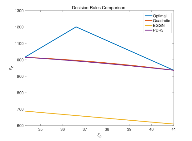
Finally, we analyze the optimal decision rules from the different approximation methods by considering an instance of robust two-item newsvendor problems. Figure 1 visualizes the decision rules from the different methods as a function of the demand $\xi_{2}$ of the second item. We observe that the quadratic function from QDR and the polynomial function from PDR3 coincide with the optimal decision rules (Optimal) at the extreme points of the uncertainty set. This implies that QDR and PDR3 can generate optimal order quantities as they anticipate for the worst-case demand scenarios. On the other hand, BGGN generates suboptimal order quantities as its decision rule function does not coincide with the extremes of the optimal decision rules. We note that the COP method does not generate any decision rules. We further remark that GWK and BGGN return the same decision rule, and thus we only plot the one from BGGN.

Refer to caption
Figure 1: Comparison of the decision rule functions from QDR, BGGN, PDR3, and GWK.

5.2 Inventory control

We next consider a multi-stage robust inventory control problem with multiple products and backlogging. A stochastic programming version of the problem is described in [45]. In this problem, we must determine sales and order policies that maximize the worst-case profit over a planning horizon of $T$ time stages. At the beginning of each time stage $t$, we observe a vector of risk factors $\boldsymbol{\xi}_{t}$ that explains the uncertainty in the current demand $D_{t,p}(\boldsymbol{\xi}_{t})$ and the unit sales price $R_{t,p}(\boldsymbol{\xi}_{t})$ of each product $p\in[P]$. After $\boldsymbol{\xi}_{t}$ is revealed at time stage $t$, we must determine the quantity $s_{t,p}$ of product $p$ to sell at the current price, the amount $o_{t,p}$ of product $p$ to replenish the inventory, and the amount $b_{t,p}$ of product $p$ to backlog to the next time stage at the unit cost $C_{b}$. The sales $s_{t,p}$ of product $p$ at time stage $t$ can only be provided by orders placed at time stage $t-1$ or earlier. We denote the inventory level at the beginning of each time stage $t$ by $I_{t}$. For simplicity, we assume that one unit of each product occupies the same amount of space and incurs periodically the same inventory holding costs $C_{h}$. The inventory level is required to remain nonnegative and is not allowed to exceed the capacity limit $\bar{I}$ throughout the planning time horizon. The inventory control problem can be stated as the MSRO problem

$$\begin{array}[]{ll}\max&\min\limits_{\boldsymbol{\xi}\in\Xi}\,\sum\limits_{t=1}^{T}\sum\limits_{p=1}^{P}\left[R_{t,p}(\boldsymbol{\xi}_{t})s_{t,p}(\boldsymbol{\xi}^{t})-C_{b}b_{t,p}(\boldsymbol{\xi}^{t})-C_{h}I_{t,p}(\boldsymbol{\xi}^{t})\right]\\ \operatorname{s.t.}&I_{1,p}(\boldsymbol{\xi}^{1})=I_{0,p}-s_{1,p}(\boldsymbol{\xi}^{1}),\ b_{1,p}(\boldsymbol{\xi}^{1})=D_{1,p}(\boldsymbol{\xi}_{1})-s_{1,p}(\boldsymbol{\xi}^{1})\ \ \ \forall\,\boldsymbol{\xi}\in\Xi,\ \forall\,p\in[P]\\ &I_{t,p}(\boldsymbol{\xi}^{t})=I_{t-1,p}(\boldsymbol{\xi}^{t-1})+o_{t,p}(\boldsymbol{\xi}^{t-1})-s_{t,p}(\boldsymbol{\xi}^{t})\ \ \ \forall\,\boldsymbol{\xi}\in\Xi,\,\forall\,p\in[P],\,\forall\,t\in[T]\backslash\{1\}\\ &b_{t,p}(\boldsymbol{\xi}^{t})=b_{t-1,p}(\boldsymbol{\xi}^{t-1})+D_{t,p}(\boldsymbol{\xi}_{t})-s_{t,p}(\boldsymbol{\xi}^{t})\ \ \ \forall\,\boldsymbol{\xi}\in\Xi,\,\forall\,p\in[P],\,\forall\,t\in[T]\backslash\{1\}\\ &o_{t,p}(\boldsymbol{\xi}^{t}),s_{t,p}(\boldsymbol{\xi}^{t}),b_{t,p}(\boldsymbol{\xi}^{t}),I_{t,p}(\boldsymbol{\xi}^{t})\geq 0,I_{t,p}(\boldsymbol{\xi}^{t})\leq\bar{I}\ \ \ \forall\,\boldsymbol{\xi}\in\Xi,\,\forall\,p\in[P],\,\forall\,t\in[T],\end{array}$$ (28)

where $I_{0,p}$ are fixed to pre-specified quantities for all $p\in[P]$. The product prices are defined as

$$R_{t,p}(\boldsymbol{\xi}_{t})=4+\alpha_{1,p}\xi_{t,1}+\alpha_{2,p}\xi_{t,2}+\alpha_{3,p}\xi_{t,3}+\alpha_{4,p}\xi_{t,4}$$

with factor loadings $\alpha_{1,p},\alpha_{2,p},\alpha_{3,p},\alpha_{4,p}\in[-1,1]$. Similarly, we set the demands to

$$D_{t,p}(\boldsymbol{\xi}_{t})=2+\sin(\frac{2\pi(t-1)}{12})+\frac{1}{2}[\beta_{1,p}\xi_{t,1}+\beta_{2,p}\xi_{t,2}+\beta_{3,p}\xi_{t,3}+\beta_{4,p}\xi_{t,4}]$$

for $p=1,\ldots,P/2$ and

$$D_{t,p}(\boldsymbol{\xi}_{t})=2+\cos(\frac{2\pi(t-1)}{12})+\frac{1}{2}[\beta_{1,p}\xi_{t,1}+\beta_{2,p}\xi_{t,2}+\beta_{3,p}\xi_{t,3}+\beta_{4,p}\xi_{t,4}]$$

for $p=1/P+1,\ldots,P$ with factor loadings $\beta_{1,p},\beta_{2,p},\beta_{3,p},\beta_{4,p}\in[-1,1]$. The sine (cosine) terms in the above expression correspond to the stylized fact that the expected demands of the first (last) P/2 products are high in spring (winter) and low in fall (summer). We assume that the vectors of risk factors $\boldsymbol{\xi}_{t}\in{\mathbb{R}}^{4}$ for all $t=1,\ldots,T$, are serially independent and uniformly distributed on $[-1,1]^{4}$. Formally, the uncertainty set is defined as

$$\Xi:=\left\{(\boldsymbol{\xi}:=\boldsymbol{\xi}_{1},\ldots,\boldsymbol{\xi}_{t}):\|\boldsymbol{\xi}_{t}\|_{\infty}\leq 1\ \forall\,t\in[T]\right\}.$$

The associated cone ${\mathcal{K}}$ is written as follows:

$${\mathcal{K}}:=\left\{(\boldsymbol{\xi},\tau)\in{\mathbb{R}}^{4T}\times{\mathbb{R}}_{+}:\|\boldsymbol{\xi}_{t}\|_{\infty}\leq\tau\ \forall\,t\in[T]\right\}.$$

In all numerical experiments, we generate $25$ random instances of the inventory control problem with $P=4$ products. We utilize the mechanism in [45] to set up the parameters and to generate the random instances. We set backlogging and inventory holding costs identically to $C_{b}=C_{h}=0.2$. We further set the initial inventory level to $I_{0,p}=0$ and the inventory capacity to $\bar{I}=24$. We sample the factor loadings $\alpha_{1,p},\alpha_{2,p},\alpha_{3,p},\alpha_{4,p}$ and $\beta_{1,p},\beta_{2,p},\beta_{3,p},\beta_{4,p}$ uniformly from the interval $[-1,1]$. As problem (28) has non-fixed recourse, we employ linear decision rules, and further enhance them by applying the piecewise scheme discussed in Section 2.4, where the folding directions are described by the standard basis vectors $\mathbf{e}_{\ell}$, $\ell\in[4]$. This gives rise to a semidefinite approximation which results from replacing the copositive cone $\mathcal{COP}({\mathcal{K}})$ in the equivalent copositive program with the inner approximation ${\mathcal{IA}}({\mathcal{K}})$ defined in (16). We compare our scheme (PLDR) with the one proposed by Ben-Tal et al. (BGGN) where we replace the cone $\mathcal{COP}({\mathcal{K}})$ with the inner approximation ${\mathcal{AS}}({\mathcal{K}})$ defined in (18), and with polynomial decision rule scheme of degree $3$ (PDR3).

We test the different schemes on problem instances with planning horizons $T=1$, $3$, $6$, $9$, $12$, $15$, $18$, $21$, and $24$. Table 4 reports the relative gaps between the optimal values of PLDR and those of the other two schemes, while Table 5 shows the average computation times for the three approximation schemes. Note that PDR3 can only solve instances up to $T=3$ before it starts experiencing numerical issues. As illustrated in Table 4, the relative gap between PLDR and BGGN increases dramatically with the planning horizon, where the largest average improvement of $191.2\%$ is observed for $T=24$. Meanwhile, PLDR can generate the same results as PDR3 in the case of $T=1$, and remain very close to PDR3 for $T=3$. As illustrated in these tables, our proposed copositive scheme can return solutions that are of very high quality without sacrificing much computational effort.

Number of time stages
Method Statistic 1 3 6 9 12 15 18 21 24
BGGN $10$th prct. 3.5 9.8 1.7 18.8 8.5 4.6 24.8 23.5 6.6
Mean 17.3 21.0 20.8 42.7 47.9 43.7 99.2 129.3 191.2
$90$th prct. 39.2 38.3 36.8 70.6 100.5 94.6 154.9 225.4 762.7
PDR3 $10$th prct. 0 0 - - - - - - -
Mean 0 -0.1 - - - - - - -
$90$th prct. 0 -0.2 - - - - - - -
Table 4: Relative gaps (in percent) between the alternative approximation schemes and PLDR
Number of time stages
Method 1 3 6 9 12 15 18 21 24
PLDR 0.02 0.29 2.31 9.66 34.60 99.29 248.40 541.75 1050.91
BGGN 0.01 0.04 0.33 1.23 4.76 14.48 36.85 94.49 191.30
PDR3 0.13 28.17 - - - - - - -
Table 5: The average computation times (in seconds) of the different approximation schemes

We also assess the quality of the decision rules obtained from the different approximation methods by evaluating their true worst-case profits. Since the inventory control problem has non-fixed recourse, the worst-case profit of a fixed decision does not necessarily correspond to an extreme point scenario of the uncertainty set $\Xi$. As a result, we design a simulation procedure to estimate the worst-case profit. Specifically, we randomly generate 10,000 samples from the uncertainty set, where each sample point corresponds to a trajectory realization of the demands and prices over the $T$ periods. The approximate worst-case profit is then given by the sample point that generates the smallest profit. Table 6 reports the statistics of relative gaps between the worst-case-scenario profit of our method and BGGN and PDR3. We find that the proposed PLDR scheme still provides substantial average improvements over BGGN method.

Number of time stages
Method Statistic 1 3 6 9 12 15 18 21 24
BGGN $10$th prct. 1.7 6.9 1.5 12.8 6.9 3.7 22.3 19.4 6.1
Mean 15.3 19.6 17.9 35.9 42.8 41.6 79.2 119.9 181.7
$90$th prct. 34.7 36.1 34.5 61.7 89.1 90.3 132.8 187.8 692.4
PDR3 $10$th prct. 0 0 - - - - - - -
Mean 0 -0.1 - - - - - - -
$90$th prct. 0 -0.1 - - - - - - -
Table 6: Relative gaps (in percent) of the worst-case-scenario profits between the alternative approximation schemes and PLDR

5.3 Index tracking

For the last example, we study a dynamic index tracking problem, which aims at matching the performance of a stock index as closely as possible with a portfolio of other financial instruments over a finite discrete planning horizon $T$. A stochastic programming version of the problem is described in [54]. To this end, we consider five stock indices, where the first four constitute the tracking instruments while the last one corresponds to the target index. Let $\boldsymbol{\xi}\in{\mathbb{R}}^{5}_{+}$ be the vector of total returns (price relatives) of these indices from time stage $t-1$ to time stage $t$. Here, $\xi_{t,1}$, $\xi_{t,2}$, $\xi_{t,3}$, and $\xi_{t,4}$ are returns of the four tracking instruments, while $\xi_{t,5}$ is return of the target index at time stage $t$. The robust dynamic index tracking problem is stated as follows:

$$\begin{array}[]{ll}\min&\max\limits_{\boldsymbol{\xi}\in\Xi}\,\sum\limits_{t=1}^{T}|\xi_{t,5}-s_{t}(\boldsymbol{\xi}^{t})|\\ \operatorname{s.t.}&\boldsymbol{x}_{0}\geq 0,\ \boldsymbol{e}^{\top}\boldsymbol{x}_{0}\leq 1,\ s_{1}(\boldsymbol{\xi}^{1})=\boldsymbol{\xi}_{1}^{\top}\boldsymbol{x}_{0}\\ &s_{t}(\boldsymbol{\xi}^{t})=\boldsymbol{\xi}_{t}^{\top}\boldsymbol{x}_{t-1}(\boldsymbol{\xi}^{t-1})\ \ \ \forall\,t\in[T]\backslash\{1\}\\ &\boldsymbol{e}^{\top}\boldsymbol{x}_{t}(\boldsymbol{\xi}^{t})\leq s_{t}(\boldsymbol{\xi}^{t}),\ \boldsymbol{x}_{t}(\boldsymbol{\xi}^{t})\geq 0\ \ \ \forall\,t\in[T],\end{array}$$ (29)

The decision variable $s_{t}(\boldsymbol{\xi}^{t})\in{\mathbb{R}}_{+}$ determines the value of the tracking portfolio at time stage $t$. Here, we aim to rebalance the portfolio allocation vector $\boldsymbol{x}(\boldsymbol{\xi}^{t})\in{\mathbb{R}}^{4}$ of the four tracking instruments such that $s_{t}(\boldsymbol{\xi}^{t})$ is as close to $\xi_{t,5}$ as possible throughout the planning time horizon. The uncertainty set $\Xi$ in (29) is specified through a factor model as follows:

$$\Xi:=\left\{\boldsymbol{\xi}:=(\boldsymbol{\xi}_{1},\ldots,\boldsymbol{\xi}_{T}):\begin{array}[]{l}\boldsymbol{\xi}_{t}=\boldsymbol{f}+\boldsymbol{F}\boldsymbol{\zeta}_{t},\ \boldsymbol{\zeta}_{t}\in{\mathbb{R}}^{3}\ \ \ \forall\,t\in[T]\\ \|\boldsymbol{\zeta}_{t}\|_{\infty}\leq 1,\ \|\boldsymbol{\zeta}_{t}\|_{1}\leq\rho\ \ \ \forall\,t\in[T]\end{array}\right\}$$

The associated cone ${\mathcal{K}}$ is accordingly written as

$${\mathcal{K}}:=\left\{\boldsymbol{\xi},\tau)\in{\mathbb{R}}^{4T}\times{\mathbb{R}}_{+}:\begin{array}[]{l}\boldsymbol{\xi}_{t}=\boldsymbol{f}\tau+\boldsymbol{F}\boldsymbol{\zeta}_{t},\ \boldsymbol{\zeta}_{t}\in{\mathbb{R}}^{3}\ \ \ \forall\,t\in[T]\\ \|\boldsymbol{\zeta}_{t}\|_{\infty}\leq\tau,\ \|\boldsymbol{\zeta}_{t}\|_{1}\leq\rho\tau\ \ \ \forall\,t\in[T]\end{array}\right\}.$$

Since the objective function of (29) is not linear, we introduce auxiliary variables $w_{t}(\cdot)$ to linearize each absolute term. This yields the multi-stage robust linear optimization problem

$$\begin{array}[]{ll}\min&\max\limits_{\boldsymbol{\xi}\in\Xi}\,\sum\limits_{t=1}^{T}w_{t}(\boldsymbol{\xi}^{t})\\ \operatorname{s.t.}&\boldsymbol{x}_{0}\geq 0,\ \boldsymbol{e}^{\top}\boldsymbol{x}_{0}\leq 1,\ s_{1}(\boldsymbol{\xi}^{1})=\boldsymbol{\xi}_{1}^{\top}\boldsymbol{x}_{0}\\ &s_{t}(\boldsymbol{\xi}^{t})=\boldsymbol{\xi}_{t}^{\top}\boldsymbol{x}_{t-1}(\boldsymbol{\xi}^{t-1})\ \ \ \forall\,t\in[T]\backslash\{1\}\\ &\boldsymbol{e}^{\top}\boldsymbol{x}_{t}(\boldsymbol{\xi}^{t})\leq s_{t}(\boldsymbol{\xi}^{t}),\ \boldsymbol{x}_{t}(\boldsymbol{\xi}^{t})\geq 0\ \ \ \forall\,t\in[T]\\ &w_{t}(\boldsymbol{\xi}^{t})\geq\xi_{t,5}-s_{t}(\boldsymbol{\xi}^{t}),\ w_{t}(\boldsymbol{\xi}^{t})\geq s_{t}(\boldsymbol{\xi}^{t})-\xi_{t,5}\ \ \ \forall\,t\in[T].\end{array}$$ (30)

As problem (30) has non-fixed recourse, we apply linear decision rules to the decision variables $\boldsymbol{x}_{t}(\cdot)$, $t\in[T]$, which are multiplied with some uncertain parameters. On the other hand, we may utilize quadratic decision rules on $s_{t}(\cdot)$ and $w_{t}(\cdot)$, $t\in[T]$, as they are not multipled with any uncertain parameters. With minimum modification, the copositive approach introduced in Section 4 can be applied and, accordingly, we can solve the semidefinite approximation which results from replacing the copositive cone $\mathcal{COP}({\mathcal{K}})$ with the inner approximation ${\mathcal{IA}}({\mathcal{K}})$ defined in (16). We denote our approach by LQDR. We compare LQDR with the scheme proposed by Ben-Tal et al. (BGGN) where we replace the cone $\mathcal{COP}({\mathcal{K}})$ with the inner approximation ${\mathcal{AS}}({\mathcal{K}})$ defined in (18), and with polynomial decision rule scheme of degree $3$ (PDR3).

All experimental results are averaged over 25 randomly generated instances. We utilize the mechanism in [54] to set up the parameters and to generate the random instances. For each instance, $\boldsymbol{f}$ is set to the vector of all ones, while each entry of $\boldsymbol{F}$ is sampled uniformly from the interval $[-1,1]$. We further normalize each row of $\boldsymbol{F}$ such that the sum of the absolute values in each row equals to 1. We test the different schemes on problem instances with planning horizons $T=1$, $3$, $6$, $9$, $12$, $15$, and $18$. Note that PDR3 can only solve instances up to $T=3$. Table 7 reports the statistics of relative gaps between the optimal values obtained from LQDR and those from the two alternative approximation schemes, while Table 8 shows the average computation times for all three approximation schemes. As indicated in Table 7, the relative gap between LQDR and BGGN increases with the planning horizon, where the largest average improvement of $18.2\%$ is observed for $T=18$. On the other hand, LQDR generates similar performance to PLDR3 but with significantly less computational effort.

Number of time stages
Method Statistic 1 3 6 9 12 15 18
BGGN $10$th prct. 0.0 1.0 1.9 2.2 4.7 1.8 2.5
Mean 0.0 7.1 12.5 11.8 14.2 17.0 18.2
$90$th prct. 0.0 21.7 29.4 29.0 33.8 30.1 34.2
PDR3 $10$th prct. 0.0 0.0 - - - - -
Mean 0.0 -0.1 - - - - -
$90$th prct. 0.0 -0.4 - - - - -
Table 7: Relative gaps (in percent) between the alternative approximation schemes and LQDR
Number of time stages
Method 1 3 6 9 12 15 18
LQDR 0.03 0.40 5.01 32.95 127.34 601.57 1703.32
BGGN 0.02 0.08 0.69 5.47 24.70 75.48 226.18
PDR3 0.09 8.50 - - - - -
Table 8: The average computation times (in seconds) of the different approximation schemes

We also assess the quality of the decision rules obtained from the different approximation methods by evaluating their worst-case risks. As in the inventory control problem, the index tracking problem has a non-fixed recourse. We adopt the same simulation procedure by using 10,000 sample trajectories from the uncertainty set to estimate the worst-case risks. Table 9 reports the statistics of relative gaps between the worst-case-scenario risk of our method and BGGN and PDR3. We find that the proposed PLDR scheme provides substantial average improvements over BGGN method.

Number of time stages
Method Statistic 1 3 6 9 12 15 18
BGGN $10$th prct. 0.0 0.1 1.2 1.6 4.2 1.4 1.9
Mean 0.0 5.2 10.4 9.7 12.1 13.7 14.1
$90$th prct. 0.0 18.5 24.2 25.2 31.0 27.4 29.2
PDR3 $10$th prct. 0.0 0.0 - - - - -
Mean 0.0 -0.0 - - - - -
$90$th prct. 0.0 -0.3 - - - - -
Table 9: Relative gaps (in percent) of the simulated worst-case-scenario risks between the alternative approximation schemes and LQDR

6 Concluding remarks

Generic MSRO problems (with non-fixed recourse) have so far resisted strong decision rule approximations. In this paper, we leveraged modern conic programming techniques to derive an exact convex copositive program for the linear decision rule approximation of these difficult optimization problems. We further derived an equivalent copositive program for the more powerful quadratic decision rule approximation of instances with fixed recourse. These reformulations enabled us to obtain a new semidefinite approximation that is provably tighter than an existing scheme of similar complexity by Ben-Tal et al. The copositive approach further inspired us to develop a new piecewise decision rule scheme for the generic problems. For MSRO problems with non-fixed recourse, we proved that the resulting approximation is tighter than the state-of-the-art scheme by Georghiou et al. Extensive numerical results demonstrate that our scheme can substantially outperform existing schemes in terms of optimality, while maintaining scalability when solving large problem instances. We conclude that our proposed copositive approach provides an excellent balance between optimality and scalability.

We mention two promising directions for further research. First, it would be interesting to derive a copositive programming reformulation for the piecewise decision rule scheme where we simultaneously optimize for the best folding directions and breakpoints. Second, it is imperative to design a global solution approach for MSRO problems with non-fixed recourse that leverages the proposed decision rule schemes.

Acknowledgements.

Grani A. Hanasusanto is supported by the National Science Foundation grant no. 1752125. The work presented in this paper was carried out while Guanglin Xu was a postdoctoral fellow at the Institute for Mathematics and its Applications during the IMA’s annual program on Modeling, Stochastic Control, Optimization, and Related Applications.

Appendix

Proof of Lemma 2

Proof.

Fix $(\boldsymbol{z},\tau)\in{\mathcal{K}}$. For the sake of contradiction, suppose that $\tau=0$ but $\boldsymbol{z}\neq 0$. By Assumption 1, the set ${\mathcal{U}^{0}}$ is nonempty. Choose any ${\boldsymbol{u}}\in{\mathcal{U}^{0}}$, so that ${\boldsymbol{u}}\in{\mathcal{K}}$ and $u_{K+1}=1$. Then, for any non-negative scalar $\rho\geq 0$, we have $\boldsymbol{w}(\rho):={\boldsymbol{u}}+\rho(\boldsymbol{z}^{\top},0)^{\top}\in{\mathcal{K}}$. Furthermore, $\boldsymbol{w}(\rho)\in{\mathcal{U}^{0}}$ as $[\boldsymbol{w}(\rho)]_{K+1}=1$. Since $\rho$ can be arbitrarily large while $\boldsymbol{z}\neq 0$, we conclude that ${\mathcal{U}^{0}}$ is unbounded, contradicting the compactness condition of Assumption 1. Thus, the claim follows. ∎

Proof of Lemma 3

Proof.

We prove the statement by showing that the dual problem (6) admits a Slater point. To this end, we set $\alpha_{i}=0$, $i\in[I]$. We then seek for a scalar $\lambda$ that ensures

$$(\boldsymbol{z}^{\top},\tau)\left(\lambda\mathbf{e}_{K+1}\mathbf{e}_{K+1}^{\top}-\boldsymbol{\widehat{C}}_{0}\right)(\boldsymbol{z}^{\top},\tau)^{\top}=\lambda\tau^{2}-(\boldsymbol{z}^{\top},\tau)\boldsymbol{\widehat{C}}_{0}(\boldsymbol{z}^{\top},\tau)^{\top}>0$$

for all non-zero vector $(\boldsymbol{z},\tau)$ in ${\mathcal{K}}$. By Lemma 2, it suffices to consider the case where $\tau>0$, in which case we may divide the expression by $\tau^{2}$. We thus require that $\lambda-((\boldsymbol{z}/\tau)^{\top},1)\boldsymbol{\widehat{C}}_{0}((\boldsymbol{z}/\tau)^{\top},1)^{\top}$ is strictly positive for all $(\boldsymbol{z},\tau)\in{\mathcal{K}}$, $\tau>0$. Since $(\boldsymbol{z},\tau)\in{\mathcal{K}}$, we have that $(\boldsymbol{z}/\tau,1)\in{\mathcal{K}}$, and, by construction, $(\boldsymbol{z}/\tau,1)\in{\mathcal{U}^{0}}$. In this case, the boundedness of ${\mathcal{U}^{0}}$ implies that there exists a constant $\lambda^{\star}$ such that $\lambda^{\star}>((\boldsymbol{z}/\tau)^{\top},1)\boldsymbol{\widehat{C}}_{0}((\boldsymbol{z}/\tau)^{\top},1)^{\top}$ for all $(\boldsymbol{z}/\tau,1)\in{\mathcal{U}^{0}}$. The claim thus follows since the point $(\lambda,\boldsymbol{\alpha})=(\lambda^{\star},\boldsymbol{0})$ constitutes a Slater point for the problem (6). ∎

Proof of Theorem 1

Proof.

Using Lemmas 1 and 3, we can reformulate the maximization problem in the objective function of (${\mathcal{L}}$) as a copositive minimization problem. To this end, for any fixed decision rule coefficients $\boldsymbol{Y}\in{\mathbb{R}}^{N\times(K+1)}$, we consider the maximization problem given by

$$\sup\limits_{{\boldsymbol{u}}\in{\mathcal{U}}}\,(\boldsymbol{\widehat{D}}{\boldsymbol{u}})^{\top}\boldsymbol{Y}{\boldsymbol{u}}.$$ (31)

By Lemma 1, the problem can be reformulated as a linear program over the cone of completely positive matrices with respect to ${\mathcal{K}}$, as follows:

$$\begin{array}[]{ll}\sup&\dfrac{1}{2}\left(\boldsymbol{\widehat{D}}^{\top}\boldsymbol{Y}+\boldsymbol{Y}^{\top}\boldsymbol{\widehat{D}}\right)\bullet\boldsymbol{U}\\ \operatorname{s.t.}&\mathbf{e}_{K+1}\mathbf{e}_{K+1}^{\top}\bullet\boldsymbol{U}=1\\ &\boldsymbol{\widehat{C}}_{i}\bullet\boldsymbol{U}=0\ \ \ \forall\,i\in[I]\\ &\boldsymbol{U}\in{\mathcal{S}}^{K+1},\ \boldsymbol{U}\in\mathcal{CP}({\mathcal{K}})\end{array}$$ (32)

Letting $\lambda$ and $\boldsymbol{\alpha}$ be the dual variables corresponding to the constraints $\mathbf{e}_{K+1}\mathbf{e}_{K+1}^{\top}\bullet\boldsymbol{U}=1$ and $\boldsymbol{\widehat{C}}_{i}\bullet\boldsymbol{U}=0$, $i\in[I]$, respectively, the dual problem is written as:

$$\begin{array}[]{ll}\inf&\lambda\\ \operatorname{s.t.}&\lambda\,\mathbf{e}_{K+1}\mathbf{e}_{K+1}^{\top}-\dfrac{1}{2}\left(\boldsymbol{\widehat{D}}^{\top}\boldsymbol{Y}+\boldsymbol{Y}^{\top}\boldsymbol{\widehat{D}}\right)+\sum\limits_{i=1}^{I}\alpha_{i}\boldsymbol{\widehat{C}}_{i}\in\mathcal{COP}({\mathcal{K}})\\ &\lambda\in{\mathbb{R}},\ \boldsymbol{\alpha}\in{\mathbb{R}}^{I}.\end{array}$$ (33)

In view of Lemma 3, strong duality holds for the primal and dual pair, i.e., the optimal value of problem (31) coincides with that of problem (33). Replacing the maximization problem in (${\mathcal{L}}$) with the minimization problem in (33) yields the objective function and the first constraint in (9).

Next, using standard techniques from robust optimization, we reformulate the semi-infinite constraints in (${\mathcal{L}}$) into a finite constraint system. By substituting the definition of problem parameters ${\boldsymbol{\mathcal{A}}}({\boldsymbol{u}})$, ${\boldsymbol{\mathcal{B}}}({\boldsymbol{u}})$, and ${\boldsymbol{h}}({\boldsymbol{u}})$, and using the definitions in (7), we can simplify the semi-infinite constraints in (${\mathcal{L}}$) to the constraints

$${\boldsymbol{u}}^{\top}\boldsymbol{\widehat{\Theta}}_{j}{\boldsymbol{x}}+{\boldsymbol{u}}^{\top}\boldsymbol{\widehat{\Lambda}}_{j}\boldsymbol{Y}{\boldsymbol{u}}\geq\boldsymbol{\widehat{h}}_{j}^{\top}{\boldsymbol{u}}\ \ \ \forall\,{\boldsymbol{u}}\in{\mathcal{U}}\ \ \forall\,j\in[J],$$

where $\boldsymbol{\widehat{\Theta}}_{j}$ and $\boldsymbol{\widehat{\Lambda}}_{j}$ are defined as in (7). For any fixed $({\boldsymbol{x}},\boldsymbol{Y})\in{\mathbb{R}}^{M}\times{\mathbb{R}}^{N\times(K+1)}$, we consider the $j$-th constraint separately, which can equivalently be stated as

$$\inf\limits_{{\boldsymbol{u}}\in{\mathcal{U}}}\,\left({\boldsymbol{u}}^{\top}\boldsymbol{\widehat{\Theta}}_{j}{\boldsymbol{x}}+{\boldsymbol{u}}^{\top}\boldsymbol{\widehat{\Lambda}}_{j}\boldsymbol{Y}{\boldsymbol{u}}-\boldsymbol{\widehat{h}}_{j}^{\top}{\boldsymbol{u}}\right)\geq 0.$$ (34)

By Lemma 1, the minimization problem on the left-hand side of (34) can be reformulated as the following linear program over the cone of completely positive matrices:

$$\begin{array}[]{ll}\inf&\boldsymbol{\Omega}_{j}(\boldsymbol{x},\,\boldsymbol{Y})\bullet\boldsymbol{U}_{j}\\ \operatorname{s.t.}&\mathbf{e}_{K+1}\mathbf{e}_{K+1}^{\top}\bullet\boldsymbol{U}_{j}=1\\ &\boldsymbol{\widehat{C}}_{i}\bullet\boldsymbol{U}_{j}=0\ \ \ \forall\,i\in[I]\\ &\boldsymbol{U}_{j}\in{\mathcal{S}}^{K+1},\ \boldsymbol{U}_{j}\in\mathcal{CP}({\mathcal{K}}).\end{array}$$ (35)

Letting $\pi_{j}\in{\mathbb{R}}$ and $\boldsymbol{\beta}_{j}\in{\mathbb{R}}^{I}$ be the dual variables corresponding to the constraints $\mathbf{e}_{K+1}\mathbf{e}_{K+1}^{\top}\bullet\boldsymbol{U}_{j}=1$ and $\boldsymbol{\widehat{C}}_{i}\bullet\boldsymbol{U}_{j}=0$, $i\in[I]$, respectively, the dual problem is given by

$$\begin{array}[]{ll}\sup&\pi_{j}\\ \operatorname{s.t.}&\boldsymbol{\Omega}_{j}(\boldsymbol{x},\,\boldsymbol{Y})-\pi_{j}\,\mathbf{e}_{K+1}\mathbf{e}_{K+1}^{\top}-\sum\limits_{i=1}^{I}[\boldsymbol{\beta}_{j}]_{i}\,\boldsymbol{\widehat{C}}_{i}\in\mathcal{COP}({\mathcal{K}})\\ &\pi_{j}\in{\mathbb{R}},\ \boldsymbol{\beta}_{j}\in{\mathbb{R}}^{I}.\end{array}$$ (36)

If the conditions in Assumption 1 hold, then by Lemmas 1 and 3, the optimal value of the left-hand side problem in (34) coincides with that of problem (36). The emerging constraint is satisfied if and only if there exists $\pi_{j}\geq 0$ and $\boldsymbol{\beta}_{j}\in{\mathbb{R}}^{I}$ such that

$$\begin{array}[]{l}\boldsymbol{\Omega}_{j}\left(\boldsymbol{x},\,\boldsymbol{Y}\right)-\pi_{j}\,\mathbf{e}_{K+1}\mathbf{e}_{K+1}^{\top}-\sum\limits_{i=1}^{I}[\boldsymbol{\beta}_{j}]_{i}\,\boldsymbol{\widehat{C}}_{i}\in\mathcal{COP}({\mathcal{K}}).\end{array}$$

Combining the result for all $J$ constraints yields the finite constraint system

$$\boldsymbol{\Omega}_{j}\left(\boldsymbol{x},\,\boldsymbol{Y}\right)-\pi_{j}\,\mathbf{e}_{K+1}\mathbf{e}_{K+1}^{\top}-\sum\limits_{i=1}^{I}[\boldsymbol{\beta}_{j}]_{i}\,\boldsymbol{\widehat{C}}_{i}\in\mathcal{COP}({\mathcal{K}}),\ \pi_{j}\geq 0\ \ \ \forall\,j\in[J],$$

which completes the proof. ∎

Proof of Theorem 2

Proof.

The proof parallels that of Theorem 1. Using Lemma 1, we reformulate the maximization problem $\sup_{{\boldsymbol{u}}\in{\mathcal{U}}}\sum_{n=1}^{N}\widehat{d}_{n}{\boldsymbol{u}}^{\top}\boldsymbol{Q}_{n}{\boldsymbol{u}}$ in the objective function of (${\mathcal{Q}}$) into a copositive minimization problem given by

$$\begin{array}[]{ll}\inf&\lambda\\ \operatorname{s.t.}&\lambda\,\mathbf{e}_{K+1}\mathbf{e}_{K+1}^{\top}-\sum\limits_{n=1}^{N}\widehat{d}_{n}\boldsymbol{Q}_{n}-\sum\limits_{i=1}^{I}\alpha_{i}\boldsymbol{\widehat{C}}_{i}\in\mathcal{COP}({\mathcal{K}})\\ &\lambda\in{\mathbb{R}},\ \boldsymbol{\alpha}\in{\mathbb{R}}^{I}.\end{array}$$

Then, replacing the maximization problem in (${\mathcal{Q}}$) with the above minimization problem yields the objective function and the first constraint in (11).

Next, we can reformulate the constraint

$${\boldsymbol{u}}^{\top}\boldsymbol{\widehat{\Theta}}_{j}{\boldsymbol{x}}+\sum\limits_{n=1}^{N}\widehat{b}_{jn}{\boldsymbol{u}}^{\top}\boldsymbol{Q}_{n}{\boldsymbol{u}}\geq\boldsymbol{\widehat{h}}_{j}^{\top}{\boldsymbol{u}}\ \ \ \forall\,{\boldsymbol{u}}\in{\mathcal{U}}$$

corresponding to the $j$-th semi-infinite constraint in (${\mathcal{Q}}$) into the equivalent constraints

$$\begin{array}[]{l}\boldsymbol{\Gamma}_{j}\left(\boldsymbol{x},\boldsymbol{Q}_{1},\ldots,\boldsymbol{Q}_{N}\right)-\pi_{j}\,\mathbf{e}_{K+1}\mathbf{e}_{K+1}^{\top}-\sum\limits_{i=1}^{I}[\boldsymbol{\beta}_{j}]_{i}\,\boldsymbol{\widehat{C}}_{i}\in\mathcal{COP}({\mathcal{K}}),\ \pi_{j}\geq 0.\end{array}$$

Combining this result for all $J$ semi-infinite constraints yields the second constraint system in (11). This completes the proof. ∎

Proof of Lemma 4

Proof.

For any ${\boldsymbol{u}}\in{\mathcal{K}}$, the second-order cone constraint $\boldsymbol{\widehat{R}}{\boldsymbol{u}}\in\mathcal{SOC}(K_{r})$ in the description of ${\mathcal{K}}$ stipulates that

$$\mathbf{e}_{K_{r}}^{\top}\boldsymbol{\widehat{R}}{\boldsymbol{u}}\geq\sqrt{(\mathbf{e}_{1}^{\top}\boldsymbol{\widehat{R}}{\boldsymbol{u}})^{2}+\cdots+(\mathbf{e}_{K_{r}-1}^{\top}\boldsymbol{\widehat{R}}{\boldsymbol{u}})^{2}}.$$ (37)

Squaring both sides of the inequality yields

$\displaystyle{\boldsymbol{u}}^{\top}\boldsymbol{\widehat{R}}^{\top}\mathbf{e}_{K_{r}}\mathbf{e}_{K_{r}}^{\top}\boldsymbol{\widehat{R}}{\boldsymbol{u}}\geq{\boldsymbol{u}}^{\top}\boldsymbol{\widehat{R}}^{\top}\mathbf{e}_{1}\mathbf{e}_{1}^{\top}\boldsymbol{\widehat{R}}{\boldsymbol{u}}+\cdots+{\boldsymbol{u}}^{\top}\boldsymbol{\widehat{R}}^{\top}\mathbf{e}_{K_{r}-1}\mathbf{e}_{K_{r}-1}^{\top}\boldsymbol{\widehat{R}}{\boldsymbol{u}}$ $\displaystyle\ \ \ \Longleftrightarrow$
$\displaystyle{\boldsymbol{u}}^{\top}\left(\boldsymbol{\widehat{R}}^{\top}\mathbf{e}_{K_{r}}\mathbf{e}_{K_{r}}^{\top}\boldsymbol{\widehat{R}}-\sum\limits_{\ell=1}^{K_{r}-1}\boldsymbol{\widehat{R}}^{\top}\mathbf{e}_{\ell}\mathbf{e}_{\ell}^{\top}\boldsymbol{\widehat{R}}\right){\boldsymbol{u}}\geq 0$ $\displaystyle\ \ \ \Longleftrightarrow$
$\displaystyle{\boldsymbol{u}}^{\top}\boldsymbol{\widehat{S}}{\boldsymbol{u}}\geq 0$

Thus, the claim follows. ∎

Proof of Proposition 1

Proof.

For any $\boldsymbol{V}\in{\mathcal{IA}}({\mathcal{K}})$, we need to show that ${\boldsymbol{u}}^{\top}\boldsymbol{V}{\boldsymbol{u}}\geq 0$ for all ${\boldsymbol{u}}\in{\mathcal{K}}$. To this end, fix any $\boldsymbol{V}\in{\mathcal{IA}}({\mathcal{K}})$ and ${\boldsymbol{u}}\in{\mathcal{K}}$. By construction, we have

$\displaystyle\ {\boldsymbol{u}}^{\top}\left(\boldsymbol{W}+\tau\boldsymbol{\widehat{S}}+\boldsymbol{\widehat{P}}^{\top}\boldsymbol{\Sigma}\boldsymbol{\widehat{P}}+\boldsymbol{\Psi}\right){\boldsymbol{u}}$
$\displaystyle=$ $\displaystyle\ {\boldsymbol{u}}^{\top}\boldsymbol{W}{\boldsymbol{u}}+\tau{\boldsymbol{u}}^{\top}\boldsymbol{\widehat{S}}{\boldsymbol{u}}+{\boldsymbol{u}}^{\top}\boldsymbol{\widehat{P}}^{\top}\boldsymbol{\Sigma}\boldsymbol{\widehat{P}}{\boldsymbol{u}}+{\boldsymbol{u}}^{\top}\left(\frac{1}{2}\boldsymbol{\widehat{P}}^{\top}\boldsymbol{\Phi}\boldsymbol{\widehat{R}}+\frac{1}{2}\boldsymbol{\widehat{R}}^{\top}\boldsymbol{\Phi}^{\top}\boldsymbol{\widehat{P}}\right){\boldsymbol{u}}$
$\displaystyle=$ $\displaystyle\ {\boldsymbol{u}}^{\top}\boldsymbol{W}{\boldsymbol{u}}+\tau{\boldsymbol{u}}^{\top}\boldsymbol{\widehat{S}}{\boldsymbol{u}}+{\boldsymbol{u}}^{\top}\boldsymbol{\widehat{P}}^{\top}\boldsymbol{\Sigma}\boldsymbol{\widehat{P}}{\boldsymbol{u}}+{\boldsymbol{u}}^{\top}\boldsymbol{\widehat{P}}^{\top}\boldsymbol{\Phi}\boldsymbol{\widehat{R}}{\boldsymbol{u}}.$

We next analyze each of the four summands separately:

  1. 1.

    Since $\boldsymbol{W}\succeq\boldsymbol{0}$, we have ${\boldsymbol{u}}^{\top}\boldsymbol{W}{\boldsymbol{u}}\geq 0$.

  2. 2.

    Since $\tau\geq 0$ and by Lemma 4, we have $\tau{\boldsymbol{u}}^{\top}\boldsymbol{\widehat{S}}{\boldsymbol{u}}\geq 0$.

  3. 3.

    Since $\boldsymbol{\widehat{P}}{\boldsymbol{u}}\geq\boldsymbol{0}$ and $\boldsymbol{\Sigma}\geq\boldsymbol{0}$, we have $(\boldsymbol{\widehat{P}}{\boldsymbol{u}})^{\top}\boldsymbol{\Sigma}(\boldsymbol{\widehat{P}}{\boldsymbol{u}})\geq 0$.

  4. 4.

    Since $\boldsymbol{\widehat{R}}{\boldsymbol{u}}$ and the vectors $\textup{Rows}(\boldsymbol{\Phi})$ belong to $\mathcal{SOC}(K_{r})$, we have $\boldsymbol{\Phi}\boldsymbol{\widehat{R}}{\boldsymbol{u}}\geq\boldsymbol{0}$ (as a second-order cone is self-dual). This further implies that ${\boldsymbol{u}}^{\top}\boldsymbol{\widehat{P}}^{\top}\boldsymbol{\Phi}\boldsymbol{\widehat{R}}{\boldsymbol{u}}=(\boldsymbol{\widehat{P}}{\boldsymbol{u}})^{\top}(\boldsymbol{\Phi}\boldsymbol{\widehat{R}}{\boldsymbol{u}})\geq 0$ as $\boldsymbol{\widehat{P}}{\boldsymbol{u}}\geq\boldsymbol{0}$.

This completes the proof. ∎

Proof of Proposition 6

Proof.

For a clear proof, we begin with the case when the piecewise linear lifting is only applied to the first coordinate axis $u_{1}$, where the breakpoints are given by $h_{1}=\underline{u}_{1}<h_{2}<\ldots<h_{L}<\overline{u}_{1}$. In this case the lifted set ${\mathcal{U}}^{\prime}$ and the set ${\mathcal{U}}^{*}$ respectively simplify to

$${\mathcal{U}}^{\prime}=\left\{(\boldsymbol{w},{\boldsymbol{u}})\in{\mathbb{R}}^{L}\times\mathcal{U}:\begin{array}[]{ll}\boldsymbol{z}\in{\mathbb{R}}_{+}^{L+1}\\ w_{\ell}=z_{\ell}-z_{\ell+1}&\ell\in[L]\\ z_{1}=u_{1}-\underline{u}_{1},\;z_{L+1}=0&\\ z_{\ell}\geq u_{1}-h_{\ell},\ \overline{u}_{1}\geq z_{\ell}&\ell\in[L+1]\\ z_{\ell}(z_{\ell}-u_{1}+h_{\ell})=0&\ell\in[L+1]\end{array}\right\},$$ (38)
$${\mathcal{U}}^{*}:=\left\{(\boldsymbol{w},{\boldsymbol{u}})\in{\mathbb{R}}^{L}\times{\mathcal{U}}:\begin{array}[]{l}\boldsymbol{z}\in{\mathbb{R}}_{+}^{L+1},\;\boldsymbol{p}\in{\mathbb{R}}_{+}^{L+1},\;\boldsymbol{r}\in{\mathbb{R}}_{+}^{L},\;U\in{\mathbb{R}}_{+}\\ \boldsymbol{Z}\in{\mathcal{S}}^{L+1},\boldsymbol{W}\in{\mathcal{S}}^{L},\ \boldsymbol{Q}\in{\mathbb{R}}^{L\times(L+1)}\\ \boldsymbol{B}\boldsymbol{z}=\boldsymbol{w},\;z_{1}=u_{1}-\underline{u}_{1},\;z_{L+1}=0\\ \boldsymbol{z}\geq u_{1}\mathbf{e}-\boldsymbol{h},\ \overline{u}_{1}\mathbf{e}\geq\boldsymbol{z}\\ \operatorname{diag}(\boldsymbol{Z})-\boldsymbol{p}+\boldsymbol{h}\circ\boldsymbol{z}=\boldsymbol{0}\\ \boldsymbol{H}\begin{pmatrix}\boldsymbol{W}&\boldsymbol{Q}&\boldsymbol{r}&\boldsymbol{w}\\ \boldsymbol{Q}^{\top}&\boldsymbol{Z}&\boldsymbol{p}&\boldsymbol{z}\\ \boldsymbol{r}^{\top}&\boldsymbol{p}^{\top}&U&u_{1}\\ \boldsymbol{w}^{\top}&\boldsymbol{z}^{\top}&u_{1}&1\end{pmatrix}\boldsymbol{H}^{\top}\geq\boldsymbol{0},\;\;\begin{pmatrix}\boldsymbol{W}&\boldsymbol{Q}&\boldsymbol{r}&\boldsymbol{w}\\ \boldsymbol{Q}^{\top}&\boldsymbol{Z}&\boldsymbol{p}&\boldsymbol{z}\\ \boldsymbol{r}^{\top}&\boldsymbol{p}^{\top}&U&u_{1}\\ \boldsymbol{w}^{\top}&\boldsymbol{z}^{\top}&u_{1}&1\end{pmatrix}\succeq\boldsymbol{0}\end{array}\right\},$$ (39)

where the matrices $\boldsymbol{B}\in{\mathbb{R}}^{L\times(L+1)}$ and $\boldsymbol{H}\in{\mathbb{R}}^{(4L+2)\times(2L+3)}$ are defined as

$$\boldsymbol{B}=\begin{pmatrix}1&-1&0&\cdots&0&0&0\\ 0&1&-1&\cdots&0&0&0\\ \vdots&\ddots&\ddots&\ddots&\ddots&\vdots&\vdots\\ 0&\cdots&\cdots&\cdots&1&-1&0\\ 0&\cdots&\cdots&\cdots&\cdots&1&-1\end{pmatrix}\qquad\textup{and}\qquad\boldsymbol{H}=\begin{pmatrix}\boldsymbol{0}&\mathbb{I}&\boldsymbol{0}&\boldsymbol{0}\\ \boldsymbol{0}&\mathbb{I}&-\mathbf{e}&\boldsymbol{h}\\ -\mathbb{I}&\boldsymbol{B}&\boldsymbol{0}&\boldsymbol{0}\\ \mathbb{I}&-\boldsymbol{B}&\boldsymbol{0}&\boldsymbol{0}\\ \end{pmatrix},$$

respectively. One can verify that a point from ${\mathcal{U}}^{\prime}$ is also a member of ${\mathcal{U}}^{*}$ since the constraints in the definition of ${\mathcal{U}}^{*}$ consist of a SDP relxation of those from ${\mathcal{U}}^{\prime}$; Ssee e.g., [29]. Furthermore, the outer approximation ${\mathcal{U}}^{**}$ simplies to:

$${{\mathcal{U}}}^{**}=\left\{(\boldsymbol{w},{\boldsymbol{u}})\in{\mathbb{R}}^{L}\times{\mathcal{U}}:\begin{array}[]{ll}\displaystyle u_{1}-\underline{u}_{1}=\sum_{\ell\in[L]}w_{\ell}&\\ h_{2}-\underline{u}_{1}\geq w_{1}&\\ (h_{\ell+1}-h_{\ell})w_{\ell-1}\geq(h_{\ell}-h_{\ell-1})w_{\ell}&\forall\ell\in[L]\setminus\{1\}\end{array}\right\}.$$ (40)

We now establish that ${\mathcal{U}}^{*}\subseteq{\mathcal{U}}^{**}$. First, the constraints $\boldsymbol{B}\boldsymbol{z}=\boldsymbol{w}$, $z_{1}=u_{1}-\underline{u}_{1}$, and $z_{L+1}=0$ in ${\mathcal{U}}^{*}$ imply that

$$\sum_{\ell\in[L]}w_{\ell}=z_{1}-z_{2}+\left[\sum_{\ell\in\{2,\dots,L\}}z_{\ell}-z_{\ell+1}\right]=u_{1}-\underline{u}_{1}.$$

Next, since $z_{2}\geq u_{1}-h_{2}$, we have that $w_{1}=z_{1}-z_{2}\leq u_{1}-\underline{u}_{1}-u_{1}+h_{2}=h_{2}-\underline{u}_{1}$. Thus, the first two constraints in ${\mathcal{U}}^{**}$ are implied by ${\mathcal{U}}^{*}$. It remains to show that the final system of inequalities in ${\mathcal{U}}^{**}$ are also implied by the constraints in ${\mathcal{U}}^{*}$. By expanding the matrix product in the penultimate constraint of ${\mathcal{U}}^{*}$, we find that $\boldsymbol{Q}=\boldsymbol{B}\boldsymbol{Z}$, and the following constraints hold:

$$\begin{array}[]{c}-\boldsymbol{r}+\boldsymbol{w}\circ\boldsymbol{h}=-\boldsymbol{B}\boldsymbol{p}+(\boldsymbol{B}\boldsymbol{z})\circ\boldsymbol{h},\ \ -\boldsymbol{p}\mathbf{e}^{\top}+\boldsymbol{Z}+\boldsymbol{z}\boldsymbol{h}^{\top}\geq\boldsymbol{0},\ \ -\boldsymbol{r}\mathbf{e}^{\top}+\boldsymbol{B}\boldsymbol{Z}+\boldsymbol{w}\boldsymbol{h}^{\top}\geq\boldsymbol{0}.\end{array}$$

Next, we perform the substitutions $\boldsymbol{p}=\operatorname{diag}(\boldsymbol{Z})+\boldsymbol{h}\circ\boldsymbol{z}$, $\boldsymbol{w}=\boldsymbol{B}\boldsymbol{z}$ and $\boldsymbol{Q}=\boldsymbol{B}\boldsymbol{Z}$ to all occurrences of $\boldsymbol{p}$, $\boldsymbol{w}$, and $\boldsymbol{Q}$, respectively, in the above constraint system. We then get $\boldsymbol{r}=\boldsymbol{B}(\operatorname{diag}(\boldsymbol{Z})+\boldsymbol{h}\circ\boldsymbol{z})$, and by further substituting this value, we arrive at the equivalent constraint system

$$\begin{array}[]{c}-(\operatorname{diag}(\boldsymbol{Z})+\boldsymbol{h}\circ\boldsymbol{z})\mathbf{e}^{\top}+\boldsymbol{Z}+\boldsymbol{z}\boldsymbol{h}^{\top}\geq\boldsymbol{0},\ -\boldsymbol{B}(\operatorname{diag}(\boldsymbol{Z})+\boldsymbol{h}\circ\boldsymbol{z})\mathbf{e}^{\top}+\boldsymbol{B}\boldsymbol{Z}+\boldsymbol{B}\boldsymbol{z}\boldsymbol{h}^{\top}\geq\boldsymbol{0}.\end{array}$$

For $\ell\in\{2,\dots,L\}$, one can show that these constraints further imply the following system of linear inequalities:

$$\begin{array}[]{rl}\mathbf{e}_{\ell-1}\mathbf{e}_{\ell+1}^{\top}\bullet\boldsymbol{Z}-\mathbf{e}_{\ell+1}\mathbf{e}_{\ell+1}^{\top}\bullet\boldsymbol{Z}+z_{\ell+1}(h_{\ell-1}-h_{\ell+1})\geq 0\\[2.84526pt] \mathbf{e}_{\ell}\mathbf{e}_{\ell+1}^{\top}\bullet\boldsymbol{Z}-\mathbf{e}_{\ell+1}\mathbf{e}_{\ell+1}^{\top}\bullet\boldsymbol{Z}+z_{\ell+1}(h_{\ell}-h_{\ell+1})\geq 0\\[2.84526pt] \mathbf{e}_{\ell-1}\mathbf{e}_{\ell+1}^{\top}\bullet\boldsymbol{Z}+\mathbf{e}_{\ell}\mathbf{e}_{\ell}^{\top}\bullet\boldsymbol{Z}-\mathbf{e}_{\ell-1}\mathbf{e}_{\ell-1}^{\top}\bullet\boldsymbol{Z}-\mathbf{e}_{\ell}\mathbf{e}_{\ell+1}^{\top}\bullet\boldsymbol{Z}+z_{\ell-1}(h_{\ell+1}-h_{\ell-1})+z_{\ell}(h_{\ell}-h_{\ell+1})\geq 0\\[2.84526pt] \mathbf{e}_{\ell-1}\mathbf{e}_{\ell}^{\top}\bullet\boldsymbol{Z}+\mathbf{e}_{\ell+1}\mathbf{e}_{\ell+1}^{\top}\bullet\boldsymbol{Z}-\mathbf{e}_{\ell}\mathbf{e}_{\ell}^{\top}\bullet\boldsymbol{Z}-\mathbf{e}_{\ell-1}\mathbf{e}_{\ell+1}^{\top}\bullet\boldsymbol{Z}+z_{\ell+1}(h_{\ell+1}-h_{\ell-1})+z_{\ell}(h_{\ell-1}-h_{\ell})\geq 0\\[2.84526pt] \mathbf{e}_{\ell}\mathbf{e}_{\ell+1}^{\top}\bullet\boldsymbol{Z}-\mathbf{e}_{\ell}\mathbf{e}_{\ell}^{\top}\bullet\boldsymbol{Z}+z_{\ell}(h_{\ell+1}-h_{\ell})\geq 0.\\[2.84526pt] \end{array}$$ (41)

We further relax the large semidefinite constraint in ${\mathcal{U}}^{*}$ into $\mathcal{O}(L)$ semidefinite constraints involving $3\times 3$ matrices, as follows:

$$\boldsymbol{M}_{\ell}:=\begin{pmatrix}\mathbf{e}_{\ell-1}\mathbf{e}_{\ell-1}^{\top}\bullet\boldsymbol{Z}&\mathbf{e}_{\ell-1}\mathbf{e}_{\ell}^{\top}\bullet\boldsymbol{Z}&\mathbf{e}_{\ell-1}\mathbf{e}_{\ell+1}^{\top}\bullet\boldsymbol{Z}\\ \mathbf{e}_{\ell-1}\mathbf{e}_{\ell}^{\top}\bullet\boldsymbol{Z}&\mathbf{e}_{\ell}\mathbf{e}_{\ell}^{\top}\bullet\boldsymbol{Z}&\mathbf{e}_{\ell}\mathbf{e}_{\ell+1}^{\top}\bullet\boldsymbol{Z}\\ \mathbf{e}_{\ell-1}\mathbf{e}_{\ell+1}^{\top}\bullet\boldsymbol{Z}&\mathbf{e}_{\ell}\mathbf{e}_{\ell+1}^{\top}\bullet\boldsymbol{Z}&\mathbf{e}_{\ell+1}\mathbf{e}_{\ell+1}^{\top}\bullet\boldsymbol{Z}\\ \end{pmatrix}\succeq\boldsymbol{0}\qquad\forall\ell\in[L+1].$$ (42)

We now show that the relaxations (41) and (42) are sufficient to imply that

$$\begin{array}[]{l}(h_{\ell+1}-h_{\ell})w_{\ell-1}\geq(h_{\ell}-h_{\ell-1})w_{\ell}\Longleftrightarrow(h_{\ell+1}-h_{\ell})z_{\ell-1}+(h_{\ell}-h_{\ell-1})z_{\ell+1}\geq(h_{\ell+1}-h_{\ell-1})w_{\ell},\end{array}$$ (43)

where the equivalence follows from the substitutions $w_{\ell-1}=z_{\ell-1}-z_{\ell}$ and $w_{\ell}=z_{\ell}-z_{\ell+1}$. In order to arrive the desired implication, we require that the optimal value of the following optimization problem is greater than or equal to 00:

inf(h+1h)z1+(hh1)z+1(h+1h1)ws.t.𝑴,z1,z, and z+1 satisfy (41) and (42).\begin{array}[]{cl}\inf&(h_{\ell+1}-h_{\ell})z_{\ell-1}+(h_{\ell}-h_{\ell-1})z_{\ell+1}-(h_{\ell+1}-h_{\ell-1})w_{\ell}\\ \operatorname{s.t.}&\boldsymbol{M}_{\ell},z_{\ell-1},z_{\ell},\text{ and }z_{\ell+1}\text{ satisfy }\eqref{eq:main_inequalities}\text{ and }\eqref{eq:relaxed_k_semidefinite}.\end{array} (44)

By weak duality, the optimal value of this problem is lower bounded by the maximization problem

$$\begin{array}[]{cl}\sup&0\\ \operatorname{s.t.}&(h_{\ell+1}-h_{\ell-1})c=(h_{\ell+1}-h_{\ell})\\ &(h_{\ell}-h_{\ell-1})d+(h_{\ell+1}-h_{\ell})c=(h_{\ell+1}-h_{\ell-1})+(h_{\ell+1}-h_{\ell})e\\ &(h_{\ell}-h_{\ell-1})+(h_{\ell+1}-h_{\ell-1})a+(h_{\ell+1}-h_{\ell})b=(h_{\ell+1}-h_{\ell-1})d\\ &\displaystyle\begin{pmatrix}c&-\frac{d}{2}&\frac{d-a-c}{2}\\ -\frac{d}{2}&{-c+d+e}&\frac{-b+c-e}{2}\\ \frac{d-a-c}{2}&\frac{-b+c-e}{2}&a+b-d\end{pmatrix}\succeq 0\\ &(a,b,c,d,e)\in{\mathbb{R}}_{+}^{5}.\end{array}$$

One can verify that the solution $(a,b,c,d,e)\in{\mathbb{R}}_{+}^{5}$ satisfying $a=c=\tfrac{h_{\ell+1}-h_{\ell}}{h_{\ell+1}-h_{\ell-1}}$, $b=\tfrac{h_{\ell+1}-h_{\ell-1}}{h_{\ell+1}-h_{\ell}}$, $d=2$, and $e=\tfrac{(h_{\ell}-h_{\ell-1})^{2}}{(h_{\ell+1}-h_{\ell-1})(h_{\ell+1}-h_{\ell})}$ is feasible to the dual problem. Thus, the optimal value of the primal problem (44) is bounded below by 00, which verifies that the constraints (41) and (42) imply (43).

The above analysis also holds to the general case when the piecewise linear lifting is applied to all coordinate axis ${\boldsymbol{u}}$. In summary, we have shown that the containment ${\mathcal{U}}^{*}\subseteq{\mathcal{U}}^{**}$ holds.

Proof of Theorem 6

Proof.

For a clear proof, we begin with the case when the piecewise linear lifting is only applied to the first coordinate axis $u_{1}$, where the breakpoints are given by $h_{1}=\underline{u}_{1}<h_{2}<\ldots<h_{L}<\overline{u}_{1}$. In this case the lifted set ${\mathcal{U}}^{\prime}$ simplifies to the one shown in (38).

We apply linear decision rules on the lifted uncertain parameters, which gives rise to the following semi-infinite linear program:

$$\begin{array}[]{rcll}&\inf&{\boldsymbol{c}}^{\top}{\boldsymbol{x}}+\sup\limits_{(\boldsymbol{w},{\boldsymbol{u}})\in{\mathcal{U}}^{\prime}}\boldsymbol{\widehat{d}}^{\top}\boldsymbol{Y}(\boldsymbol{w}^{\top},\boldsymbol{u}^{\top})^{\top}\\ &\operatorname{s.t.}&{\boldsymbol{\mathcal{A}}}^{\prime}({\boldsymbol{v}}){\boldsymbol{x}}+\boldsymbol{\widehat{B}}\boldsymbol{Y}(\boldsymbol{w}^{\top},\boldsymbol{u}^{\top})^{\top}\geq{\boldsymbol{h}}^{\prime}({\boldsymbol{v}})\ \ \ \forall\,\boldsymbol{v}:=(\boldsymbol{w},{\boldsymbol{u}})\in{\mathcal{U}}^{\prime}\\ &&{\boldsymbol{x}}\in{\mathcal{X}},\,\boldsymbol{Y}\in{\mathbb{R}}^{N\times(L+K+1)}.\end{array}$$ (45)

Consider the worst-case maximization problem in the objective function of (45). For a fixed decision rule coefficient matrix $\boldsymbol{Y}$, let us denote its optimal value by $v(\boldsymbol{Y})$. That is,

$$v(\boldsymbol{Y})=\sup\limits_{(\boldsymbol{w},{\boldsymbol{u}})\in{\mathcal{U}}^{\prime}}\,\boldsymbol{\widehat{d}}^{\top}\boldsymbol{Y}(\boldsymbol{w}^{\top},\boldsymbol{u}^{\top})^{\top}.$$ (46)

Replacing the set ${\mathcal{U}}^{\prime}$ with the outer approximation given by (40) yields the upper bound $v^{**}(\boldsymbol{Y})\geq v(\boldsymbol{Y})$. A tractable finite reformulation can then be derived by virtue of standard dualization technique in robust optimization.

Alternatively, by applying Proposition 3 to the lifted set ${\mathcal{U}}^{\prime}$ in (38) and using Lemma 1, we arrive at the equivalent completely positive program

$$\begin{array}[]{rrl}v(\boldsymbol{Y})=&\sup&\boldsymbol{\widehat{d}}^{\top}\boldsymbol{Y}(\boldsymbol{w}^{\top},\boldsymbol{u}^{\top})^{\top}\\ &\operatorname{s.t.}&\mathbf{e}_{K+1}\mathbf{e}_{K+1}^{\top}\bullet\boldsymbol{U}^{\prime}=1\\ &&\mathbf{e}_{\ell}\mathbf{e}_{\ell}^{\top}\bullet\boldsymbol{Z}^{\prime}-\mathbf{e}_{\ell}\mathbf{e}_{1}^{\top}\boldsymbol{\bullet}\boldsymbol{P}^{\prime}+h_{\ell}\mathbf{e}_{\ell}\mathbf{e}_{K+1}^{\top}\bullet\boldsymbol{P}^{\prime}=0\ \ \ \forall\,\ell\in[L+1]\\ &&\begin{pmatrix}\boldsymbol{W}^{\prime}&\boldsymbol{Q}^{\prime}&\boldsymbol{R}^{\prime}\\ (\boldsymbol{Q}^{\prime})^{\top}&\boldsymbol{Z}^{\prime}&\boldsymbol{P}^{\prime}\\ (\boldsymbol{R}^{\prime})^{\top}&(\boldsymbol{P}^{\prime})^{\top}&\boldsymbol{U}^{\prime}\end{pmatrix}\in\mathcal{CP}({\mathcal{K}}^{\prime}),\ \boldsymbol{u}=\boldsymbol{U}^{\prime}\mathbf{e}_{K+1},\ \boldsymbol{w}=\boldsymbol{R}^{\prime}\mathbf{e}_{K+1}\\ &&\boldsymbol{U}^{\prime}\in{\mathcal{S}}^{K+1},\;\boldsymbol{Z}^{\prime}\in{\mathcal{S}}^{L+1},\;\boldsymbol{W}^{\prime}\in{\mathcal{S}}^{L}\\ &&\boldsymbol{P}^{\prime}\in\mathbb{R}^{(L+1)\times(K+1)},\;\boldsymbol{R}^{\prime}\in\mathbb{R}^{L\times(K+1)},\;\boldsymbol{Q}^{\prime}\in\mathbb{R}^{L\times L+1},\end{array}$$ (47)

where the cone $\mathcal{K}^{\prime}$ is defined as

$${\mathcal{K}}^{\prime}:=\left\{\begin{array}[]{l}(\boldsymbol{w},\boldsymbol{z},{\boldsymbol{u}})\in{\mathbb{R}}^{L}\times{\mathbb{R}}_{+}^{L+1}\times{\mathcal{K}}:\begin{array}[]{ll}\quad w_{\ell}=z_{\ell}-z_{\ell+1}&\ell\in[L]\\ \quad z_{1}=u_{1}-\underline{u}_{1},\;z_{L+1}=0\\ \quad z_{\ell}\geq u_{1}-h_{\ell}u_{K+1},\;\overline{u}_{1}u_{K+1}\geq z_{\ell}&\ell\in[L+1]\end{array}\end{array}\right\}.$$

An upper bound to $v(\boldsymbol{Y})$ is then obtained by replacing the completely positive cone $\mathcal{CP}({\mathcal{K}}^{\prime})$ in (47) with a valid semidefinite-representable outer approximation. To this end, we further loosen the relaxation by considering only those constraints that are independent across dimensions. We then obtain an outer approximation defined by  (39) to the feasible set of decision variables $\boldsymbol{u}$ and $\boldsymbol{w}$ in (47). Using ${\mathcal{U}}^{*}$ to replace ${\mathcal{U}}$ in (46), we arrive at another upper bound ${v}^{*}(\boldsymbol{Y})\geq v(\boldsymbol{Y})$. As the resulting maximization problem admits a Slater point, a tractable finite reformulation can then be obtained by applying standard conic duality. By Proposition 6, we establish that ${\mathcal{U}}^{*}\subseteq{\mathcal{U}}^{**}$, which, in turn, establises that $v^{*}(\boldsymbol{Y})\leq v^{**}(\boldsymbol{Y})$.

The above analysis also holds to the general case when the piecewise linear lifting is applied to all coordinate axis ${\boldsymbol{u}}$. Thus, the claim follows. ∎

References

  • [1] Farid Alizadeh and Donald Goldfarb. Second-order cone programming. Mathematical programming, 95(1):3–51, 2003.
  • [2] Brian DO Anderson and John B Moore. Optimal Control: Linear Quadratic Methods. Courier Corporation, 2007.
  • [3] MOSEK ApS. The MOSEK optimization toolbox for MATLAB manual. Version 8.0., 2016.
  • [4] Amir Ardestani-Jaafari and Erick Delage. Linearized robust counterparts of two-stage robust optimization problems with applications in operations management. INFORMS Journal on Computing, 2020.
  • [5] Alper Atamtürk and Muhong Zhang. Two-stage robust network flow and design under demand uncertainty. Operations Research, 55(4):662–673, 2007.
  • [6] Dimitra Bampou and Daniel Kuhn. Scenario-free stochastic programming with polynomial decision rules. In Decision and Control and European Control Conference (CDC-ECC), 2011 50th IEEE Conference on, pages 7806–7812. IEEE, 2011.
  • [7] Alberto Bemporad, Francesco Borrelli, and Manfred Morari. Min-max control of constrained uncertain discrete-time linear systems. IEEE Transactions on automatic control, 48(9):1600–1606, 2003.
  • [8] Aharon Ben-Tal, Laurent El Ghaoui, and Arkadi Nemirovski. Robust optimization. Princeton University Press, 2009.
  • [9] Aharon Ben-Tal, Omar El Housni, and Vineet Goyal. A tractable approach for designing piecewise affine policies in two-stage adjustable robust optimization. Mathematical Programming, 182(1):57–102, 2020.
  • [10] Aharon Ben-Tal, Boaz Golany, Arkadi Nemirovski, and Jean-Philippe Vial. Retailer-supplier flexible commitments contracts: A robust optimization approach. Manufacturing & Service Operations Management, 7(3):248–271, 2005.
  • [11] Aharon Ben-Tal, Alexander Goryashko, Elana Guslitzer, and Arkadi Nemirovski. Adjustable robust solutions of uncertain linear programs. Mathematical Programming, 99(2):351–376, 2004.
  • [12] Aharon Ben-Tal, Tamar Margalit, and Arkadi Nemirovski. Robust modeling of multi-stage portfolio problems. In High performance optimization, pages 303–328. Springer, 2000.
  • [13] Aharon Ben-Tal and Arkadi Nemirovski. Robust solutions of uncertain linear programs. Operations research letters, 25(1):1–13, 1999.
  • [14] Aharon Ben-Tal and Arkadi Nemirovski. Robust optimization–methodology and applications. Mathematical Programming, 92(3):453–480, 2002.
  • [15] Dimitris Bertsimas, David B Brown, and Constantine Caramanis. Theory and applications of robust optimization. SIAM review, 53(3):464–501, 2011.
  • [16] Dimitris Bertsimas and Frans JCT de Ruiter. Duality in two-stage adaptive linear optimization: Faster computation and stronger bounds. INFORMS Journal on Computing, 28(3):500–511, 2016.
  • [17] Dimitris Bertsimas and Iain Dunning. Multistage robust mixed-integer optimization with adaptive partitions. Operations Research, 64(4):980–998, 2016.
  • [18] Dimitris Bertsimas and Angelos Georghiou. Design of near optimal decision rules in multistage adaptive mixed-integer optimization. Operations Research, 63(3):610–627, 2015.
  • [19] Dimitris Bertsimas and Angelos Georghiou. Binary decision rules for multistage adaptive mixed-integer optimization. Mathematical Programming, 167(2):395–433, 2018.
  • [20] Dimitris Bertsimas and Vineet Goyal. On the power and limitations of affine policies in two-stage adaptive optimization. Mathematical programming, 134(2):491–531, 2012.
  • [21] Dimitris Bertsimas, Vineet Goyal, and Brian Y Lu. A tight characterization of the performance of static solutions in two-stage adjustable robust linear optimization. Mathematical Programming, 150(2):281–319, 2015.
  • [22] Dimitris Bertsimas, Dan A Iancu, and Pablo A Parrilo. Optimality of affine policies in multistage robust optimization. Mathematics of Operations Research, 35(2):363–394, 2010.
  • [23] Dimitris Bertsimas, Dan Andrei Iancu, and Pablo A Parrilo. A hierarchy of near-optimal policies for multistage adaptive optimization. IEEE Transactions on Automatic Control, 56(12):2809–2824, 2011.
  • [24] Dimitris Bertsimas, Eugene Litvinov, Xu Andy Sun, Jinye Zhao, and Tongxin Zheng. Adaptive robust optimization for the security constrained unit commitment problem. IEEE Transactions on Power Systems, 28(1):52–63, 2013.
  • [25] I. M. Bomze and E. de Klerk. Solving standard quadratic optimization problems via linear, semidefinite and copositive programming. Journal of Global Optimization, 24(2):163–185, 2002.
  • [26] Immanuel M Bomze. Copositive optimization–recent developments and applications. European Journal of Operational Research, 216(3):509–520, 2012.
  • [27] Immanuel M Bomze, Mirjam Dür, Etienne De Klerk, Cornelis Roos, Arie J Quist, and Tamás Terlaky. On copositive programming and standard quadratic optimization problems. Journal of Global Optimization, 18(4):301–320, 2000.
  • [28] Samuel Burer. On the copositive representation of binary and continuous nonconvex quadratic programs. Mathematical Programming, 120(2):479–495, 2009.
  • [29] Samuel Burer. Copositive programming. In Handbook on semidefinite, conic and polynomial optimization, pages 201–218. Springer, 2012.
  • [30] Samuel Burer. A gentle, geometric introduction to copositive optimization. Mathematical Programming, 151(1):89–116, 2015.
  • [31] Samuel Burer and Hongbo Dong. Representing quadratically constrained quadratic programs as generalized copositive programs. Operations Research Letters, 40:203–206, 2012.
  • [32] Giuseppe Carlo Calafiore. Multi-period portfolio optimization with linear control policies. Automatica, 44(10):2463–2473, 2008.
  • [33] Jieqiu Chen and Samuel Burer. Globally solving nonconvex quadratic programming problems via completely positive programming. Mathematical Programming Computation, 4(1):33–52, 2012.
  • [34] Xin Chen, Melvyn Sim, and Peng Sun. A robust optimization perspective on stochastic programming. Operations Research, 55(6):1058–1071, 2007.
  • [35] Xin Chen, Melvyn Sim, Peng Sun, and Jiawei Zhang. A linear decision-based approximation approach to stochastic programming. Operations Research, 56(2):344–357, 2008.
  • [36] Xin Chen and Yuhan Zhang. Uncertain linear programs: Extended affinely adjustable robust counterparts. Operations Research, 57(6):1469–1482, 2009.
  • [37] George B Dantzig and Gerd Infanger. Multi-stage stochastic linear programs for portfolio optimization. Annals of Operations Research, 45(1):59–76, 1993.
  • [38] E. de Klerk and D. V. Pasechnik. Approximation of the stability number of a graph via copositive programming. SIAM Journal on Optimization, 12(4):875–892, 2002.
  • [39] Seyed Hossein Hashemi Doulabi, Patrick Jaillet, Gilles Pesant, and Louis-Martin Rousseau. Exploiting the structure of two-stage robust optimization models with integer adversarial variables. Manuscript, MIT, 2016.
  • [40] Mirjam Dür. Copositive programming—a survey. Recent advances in optimization and its applications in engineering, 320, 2010.
  • [41] G. Eichfelder and J. Jahn. Set-semidefinite optimization. Journal of Convex Analysis, 15:767–801, 2008.
  • [42] Michael R Garey and David S Johnson. Computers and intractability, volume 29. W. H. Freeman and Company San Francisco, 1979.
  • [43] Angelos Georghiou, Angelos Tsoukalas, and Wolfram Wiesemann. Robust dual dynamic programming.
  • [44] Angelos Georghiou, Angelos Tsoukalas, and Wolfram Wiesemann. A primal-dual lifting scheme for two-stage robust optimization. 2017.
  • [45] Angelos Georghiou, Wolfram Wiesemann, and Daniel Kuhn. Generalized decision rule approximations for stochastic programming via liftings. Mathematical Programming, 152(1-2):301–338, 2015.
  • [46] Angelos Georghiou, Wolfram Wiesemann, and Daniel Kuhn. Wind of change: Meeting the uk’s renewable energy targets. 2015.
  • [47] Joel Goh and Melvyn Sim. Distributionally robust optimization and its tractable approximations. Operations research, 58(4-part-1):902–917, 2010.
  • [48] Can Gokalp, Areesh Mittal, and Grani Hanasusanto. Robust quadratic programming with mixed-integer uncertainty. Optimization Online, 2018.
  • [49] Chrysanthos E Gounaris, Wolfram Wiesemann, and Christodoulos A Floudas. The robust capacitated vehicle routing problem under demand uncertainty. Operations Research, 61(3):677–693, 2013.
  • [50] Elana Guslitser. Uncertainty-immunized solutions in linear programming. PhD thesis, Citeseer, 2002.
  • [51] M. J. Hadjiyiannis, P. J. Goulart, and D. Kuhn. A scenario approach for estimating the suboptimality of linear decision rules in two-stage robust optimization. In 50th IEEE conference on decision and control and European control conference (CDC-ECC), Orlando, FL, USA, December 12-15 2011.
  • [52] Grani A Hanasusanto and Daniel Kuhn. Conic programming reformulations of two-stage distributionally robust linear programs over wasserstein balls. Operations Research, 66(3):849–869, 2018.
  • [53] Grani A Hanasusanto, Daniel Kuhn, Stein W Wallace, and Steve Zymler. Distributionally robust multi-item newsvendor problems with multimodal demand distributions. Mathematical Programming, 152(1-2):1–32, 2015.
  • [54] Grani Adiwena Hanasusanto and Daniel Kuhn. Robust data-driven dynamic programming. In Advances in Neural Information Processing Systems, pages 827–835, 2013.
  • [55] Dan A Iancu, Mayank Sharma, and Maxim Sviridenko. Supermodularity and affine policies in dynamic robust optimization. Operations Research, 61(4):941–956, 2013.
  • [56] Qingxia Kong, Chung-Yee Lee, Chung-Piaw Teo, and Zhichao Zheng. Scheduling arrivals to a stochastic service delivery system using copositive cones. Operations research, 61(3):711–726, 2013.
  • [57] Daniel Kuhn, Wolfram Wiesemann, and Angelos Georghiou. Primal and dual linear decision rules in stochastic and robust optimization. Mathematical Programming, 130(1):177–209, 2011.
  • [58] J. B. Lasserre. Convexity in semialgebraic geometry and polynomial optimization. SIAM Journal on Optimization, 19(4):1995–2014, 2009.
  • [59] Johan Lofberg. Yalmip: A toolbox for modeling and optimization in matlab. In Computer Aided Control Systems Design, 2004 IEEE International Symposium on, pages 284–289. IEEE, 2004.
  • [60] Paula Cristina Martins da Silva Rocha. Medium-Term Planning in Deregulated Energy Markets with Decision Rules. PhD thesis.
  • [61] Karthik Natarajan and Chung-Piaw Teo. On reduced semidefinite programs for second order moment bounds with applications. Mathematical Programming, 161(1-2):487–518, 2017.
  • [62] Karthik Natarajan, Chung Piaw Teo, and Zhichao Zheng. Mixed 0-1 linear programs under objective uncertainty: A completely positive representation. Operations research, 59(3):713–728, 2011.
  • [63] P. A. Parrilo. Structured semidefinite programs and semialgebraic geometry methods in robustness and optimization. PhD thesis, California Institute of Technology, 2000.
  • [64] Krzysztof Postek and Dick den Hertog. Multistage adjustable robust mixed-integer optimization via iterative splitting of the uncertainty set. INFORMS Journal on Computing, 28(3):553–574, 2016.
  • [65] Paula Rocha and Daniel Kuhn. Multistage stochastic portfolio optimisation in deregulated electricity markets using linear decision rules. European Journal of Operational Research, 216(2):397–408, 2012.
  • [66] Chuen-Teck See and Melvyn Sim. Robust approximation to multiperiod inventory management. Operations research, 58(3):583–594, 2010.
  • [67] Guanglin Xu and Samuel Burer. A copositive approach for two-stage adjustable robust optimization with uncertain right-hand sides. Computational Optimization and Applications, 70(1):33–59, 2018.
  • [68] Bo Zeng and Long Zhao. Solving two-stage robust optimization problems using a column-and-constraint generation method. Operations Research Letters, 41(5):457–461, 2013.
  • [69] Jianzhe Zhen, Dick Den Hertog, and Melvyn Sim. Adjustable robust optimization via fourier–motzkin elimination. Operations Research, 66(4):1086–1100, 2018.