Active modes and dynamical balances in MRI-turbulence of Keplerian disks with a net vertical magnetic field

Abstract

We studied dynamical balances in magnetorotational instability (MRI) turbulence with net vertical field in the shearing box model of disks. Analyzing the turbulence dynamics in Fourier (${\bf k}$-)space, we identified three types of active modes that define turbulence characteristics. These modes have lengths similar to the box size, i.e., lie in the small wavenumber region in Fourier space labeled the vital area and are: (i) the channel mode – uniform in the disk plane with the smallest vertical wavenumber, (ii) the zonal flow mode – azimuthally and vertically uniform with the smallest radial wavenumber and (iii) the rest modes. The rest modes comprise those harmonics in the vital area whose energies reach more than $50\%$ of the maximum spectral energy. The rest modes individually are not so significant compared to the channel and zonal flow modes, however, the combined action of their multitude is dominant over these two modes. These three mode types are governed by interplay of the linear and nonlinear processes, leading to their interdependent dynamics. The linear processes consist in disk flow nonmodality-modified classical MRI with a net vertical field. The main nonlinear process is transfer of modes over wavevector angles in Fourier space – the transverse cascade. The channel mode exhibits episodic bursts supplied by linear MRI growth, while the nonlinear processes mostly oppose this, draining the channel energy and redistributing it to the rest modes. As for the zonal flow, it does not have a linear source and is fed by nonlinear interactions of the rest modes.

1 Introduction

Anisotropic turbulence offers a means of enhanced transport of angular momentum in astrophysical disks (Shakura & Sunyaev, 1973; Lynden-Bell & Pringle, 1974), whereas isotropic turbulence is unable to ensure such a transport. It is not surprising that from the 1980s, research in astrophysical disks focused on identifying sources of turbulence and understanding its statistical characteristics. The turning point was the beginning of the 1990s, when a linear instability mediated by a weak vertical magnetic field in differentially rotating conducting fluids (Velikhov, 1959; Chandrasekhar, 1960) – subsequently named as the magnetorotational instability (MRI) – was rediscovered for sufficiently ionized astrophysical disks by Balbus & Hawley (1991). MRI is a robust dynamical instability that leads to the exponential growth of axisymmetric perturbations, gives rise to and steadily supplies with energy magnetohydrodynamic (MHD) turbulence, as was demonstrated in earlier numerical simulations shortly after the significance of linear MRI in disks had been realized (e.g., Hawley & Balbus, 1991, 1992; Hawley et al., 1995; Brandenburg et al., 1995; Balbus & Hawley, 1998).

The generic nonnormality (non-self-adjointness) of a strongly sheared Keplerian flow of astrophysical disks provides an additional important linear mechanism of energy supply to the turbulence - transient, or nonmodal growth of perturbations (Lominadze et al., 1988; Chagelishvili et al., 2003; Yecko, 2004; Afshordi et al., 2005; Tevzadze et al., 2008; Shtemler et al., 2011; Salhi et al., 2012; Pessah & Chan, 2012; Mamatsashvili et al., 2013; Zhuravlev & Razdoburdin, 2014; Squire & Bhattacharjee, 2014; Razdoburdin & Zhuravlev, 2017). Although the nonmodal growth is generally less powerful than the classical (exponentially growing) MRI, it is nevertheless capable of driving quite robust MHD turbulence when the latter is absent, for instance, in disks threaded by a purely azimuthal/toroidal magnetic field (e.g., Hawley et al., 1995; Fromang & Nelson, 2006; Simon & Hawley, 2009; Guan et al., 2009; Guan & Gammie, 2011; Flock et al., 2012; Nauman & Blackman, 2014; Meheut et al., 2015; Gogichaishvili et al., 2017). In such spectrally, or modally stable magnetized disk flows lacking exponentially growing MRI modes, nonlinear processes are vital for turbulence sustenance. In this situation, the canonical – direct and inverse – cascade processes in classical Kolmogorov or Iroshnikov-Kraichnan phenomenologies are not capable of sustaining the turbulence – this role is taken over by a new kind of the cascade process, so-called the nonlinear transverse cascade (Horton et al., 2010; Mamatsashvili et al., 2014). What is the physical reason for the emergence of the transverse cascade in shear flows and its specific nature? The thing is that the anisotropy of the nonnormality/shear-induced linear nonmodal dynamics entails the anisotropy of the nonlinear processes – transverse, or angular redistribution of perturbation harmonics in Fourier (wavenumber) space. In spectrally stable shear flows, in which the only mechanism for the energy supply to perturbations is the linear transient growth process, the nonlinear transverse cascade, by transferring the harmonics over wavevector angles (i.e., changing the orientation of their wavevectors), continually replenishes those areas in Fourier space where they can experience transient amplification (Mamatsashvili et al., 2014, 2016). In this way, the transverse cascade guarantees a long-time sustenance of the turbulence. In the absence of such a feedback, non-axisymmetric modes that undergo in this case the most effective nonmodal transient growth, get eventually sheared away and decay. In the context of disks, this process was studied in detail in our recent paper Gogichaishvili et al. (2017) (Paper I) for the above-mentioned case of the Keplerian shear flow with a net azimuthal magnetic field by combining direct simulations of the turbulence and, based on them, the subsequent analysis of the dynamical processes in Fourier space.

In this paper, we consider a Keplerian disk threaded by a net vertical/poloidal magnetic field, where there exists classical MRI with an exponential growth of axisymmetric modes (Balbus & Hawley, 1991, 1998; Wardle, 1999; Pessah et al., 2006; Lesur & Longaretti, 2007; Pessah & Chan, 2008; Longaretti & Lesur, 2010; Latter et al., 2015; Shakura & Postnov, 2015). Because of this, there is no deficit in energy supply and the role of nonlinearity in the sustenance of perturbations is not as vital as in the case of azimuthal field. However, at the same time, MRI also owes its existence to the shear of disk flow and therefore is inevitably subject to nonmodal effects (Mamatsashvili et al., 2013; Squire & Bhattacharjee, 2014). As demonstrated in this paper, this has two important consequences. First, the nonmodally-modified, or for short nonmodal MRI growth of both axisymmetric and non-axisymmetric modes during finite times are in fact more important in the energy supply process of turbulence, because the main time scales involved are of the order of dynamical/orbital time (Walker et al., 2016), than the modal (exponential) growth of axisymmetric modes prevalent at large times (see also Squire & Bhattacharjee, 2014). Second, underlying nonlinear processes are necessarily anisotropic in Fourier space as a result of the inherent anisotropy of linear nonmodal dynamics due to the shear. This anisotropy first of all gives rise to the nonlinear transverse cascade and one of the main goals of the present paper is to vividly demonstrate its importance in forming the overall dynamical picture of net vertical field MRI-turbulence.

Recently, Murphy & Pessah (2015) investigated the saturation of MRI in disks with a net vertical field and the properties of the ensuing MHD turbulence both in physical and Fourier space. Their study was mainly devoted to characterizing the anisotropic nature of this turbulence. They also pointed out a general lack of analysis of the anisotropy in the existing literature on MRI-turbulence: “Although there have been many studies of the linear phase of the MRI and its nonlinear evolution, only a fraction have explored the mechanism responsible for its saturation in detail, and none have focused explicitly on the evolution of the degree of anisotropy exhibited by the magnetized flow as it evolves from the linear regime of the instability to the ensuing turbulent state”. The main reason for overlooking the anisotropic nature of MRI-driven turbulence in most of previous works that focused on its spectral dynamics (e.g., Fromang & Papaloizou, 2007; Simon et al., 2009; Davis et al., 2010; Lesur & Longaretti, 2011) was a somewhat misleading mathematical treatment, specifically, spherical shell-averaging procedure in Fourier space (borrowed from forced MHD turbulence studies without shear flow, see e.g., Verma, 2004; Alexakis et al., 2007), which had been employed to extract statistical information about the properties of MRI-turbulence. Obviously, the use of the shell-averaging technique, which in fact smears out the transverse cascade, is, strictly speaking, justified for isotropic turbulence, but by no means for shear flow turbulence and therefore for, its special case, MRI-turbulence “nourished” in a sheared environment of disk flow. Thus, the shell-averaging is not an optimal tool for analyzing spectra as well as dynamical processes in Fourier space that underlie MRI-driven turbulence and are far from isotropic due to the shear (see also Hawley et al., 1995; Nauman & Blackman, 2014; Lesur & Longaretti, 2011; Murphy & Pessah, 2015, Paper I). This fact also calls into question those investigations based on the shell-averaging that aim to identify a power-law character and associated slopes of turbulent energy spectrum, because the anisotropy of the energy spectrum itself, a direct consequence of the transverse cascade, is wiped out in these cases. This is perhaps the reason why the kinetic and magnetic energy spectra do not generally exhibit a well-defined power-law behavior in MRI-turbulence in disk flows with a net vertical field (Simon et al., 2009; Lesur & Longaretti, 2011; Meheut et al., 2015; Walker et al., 2016).

In view of the above, in this work we focus on the dynamics and balances in MRI-turbulence with a net vertical field. We adopt the local shearing box model of the disk with constant vertical thermal stratification. The analysis is performed in three-dimensional (3D) Fourier space in full, i.e., without doing the averaging of spectral quantities over spherical shells of given wavenumber magnitude $k=|{\bf k}|$. This allows us to capture the spectral anisotropy of the MRI-turbulence due to the shear and the resulting nonlinear angular redistribution of perturbation modes in Fourier space, i.e., transverse cascade, thereby getting a deeper understanding of spectral and statistical properties of the turbulence. In previous relevant studies on a net vertical field MRI (e.g., Goodman & Xu, 1994; Hawley et al., 1995; Sano & Inutsuka, 2001; Lesur & Longaretti, 2007; Bodo et al., 2008; Latter et al., 2009, 2010; Simon et al., 2009; Pessah & Goodman, 2009; Longaretti & Lesur, 2010; Pessah, 2010; Bai & Stone, 2014; Murphy & Pessah, 2015), this redistribution (scatter) of modes over wavevector orientations (angles) in Fourier space was attributed to secondary, or parasitic instabilities. Specifically, the most unstable, exponentially growing axisymmetric MRI modes (channels) are subject to secondary instabilities of non-axisymmetric modes with growth rates proportional to the amplitude of these channel solutions. In this way, the parasitic instabilities redistribute the energy from the primary axisymmetric channel modes to non-axisymmetric parasitic ones, halting the exponential growth of the former and leading to the saturation of MRI. Several approximations are made in this description: 1. the large amplitude channel mode is a time-independent background on which the small-amplitude parasitic modes feed and 2. the effects of the imposed vertical field, the Coriolis force, and the basic Keplerian shear are all usually neglected. These assumptions clearly simplify the analysis of the excitation and dynamics of the non-axisymmetric parasitic modes, but, more importantly, because of neglecting the basic flow shear, omit independent from the primary MRI modes source of their support - the nonmodal growth of non-axisymmetric modes, which, as discussed above, is an inevitable linear process in shear (disk) flows.

To keep an analysis general and self-consistent, together with the nonmodal growth process, we employ the concept of the nonlinear transverse cascade in the present problem of MRI with a net vertical magnetic field that naturally encompasses the secondary instabilities too. This unifying framework enables us to correctly describe the interaction between the channel and non-axisymmetric “parasitic” modes when the above assumptions break down – the amplitudes of these two mode types become comparable, so that it is no longer possible to clearly distinguish between the channel as a primary background and parasites as small perturbations on top of that. This is the case in the developed turbulent state of vertical field MRI, where channels undergo recurrent amplifications (bursts) and decays (e.g., Sano & Inutsuka, 2001; Lesur & Longaretti, 2007; Bodo et al., 2008; Simon et al., 2009; Murphy & Pessah, 2015). This decay phase is usually attributed to the linear non-axisymmetric parasitic instabilities, however, in the fully developed turbulent state it is more likely governed by nonlinearity. As is shown in this paper, the transverse cascade accounts for the transfer of energy from the axisymmetric channel modes to a broad spectrum of non-axisymmetric ones (referred to as the rest modes here) as well as to the axisymmetric zonal flow mode, which appears to commonly accompany MRI-turbulence (Johansen et al., 2009; Simon et al., 2012; Bai & Stone, 2014). The nonlinear transverse cascade may not be the vital source of the energy supply to turbulence in the presence of purely exponentially growing MRI, but still it shapes the dynamics, sets the saturation level and determines the overall “design” of the turbulence the “building blocks” of which are these three types of perturbation modes analyzed in this paper.

In the spirit of our recent works (Horton et al., 2010; Mamatsashvili et al., 2014, 2016, Paper I), here we investigate in detail the roles of underlying different anisotropic linear and nonlinear dynamical processes shaping the net vertical field MRI-turbulence. Namely, we first perform numerical simulations of the turbulence and then, using the simulation data, explicitly calculate individual linear and nonlinear terms and explore their action in Fourier space. The underlying physics, active modes and dynamical balances of the net vertical field MRI-turbulence in disks are, however, entirely different from those of the net azimuthal field one studied in Paper I, primarily because energy sources for the turbulence in these two field configurations differ in essence: in the first case, the turbulence is mostly supplied by the (nonmodally-modified) exponentially growing MRI, while in the second case just by transient growth of non-axisymmetric modes.

The present study can be regarded as a generalization of the related works by Simon et al. (2009); Lesur & Longaretti (2011), where the dynamics of vertical field MRI-turbulence – the spectra of energy, injection and nonlinear transfers – were analyzed in Fourier space, however, using a restrictive approach of shell-averaging, which misses out the shear-induced anisotropy of the turbulence and hence the interaction of axisymmetric channel and non-axisymmetric modes. It also extends the study of Murphy & Pessah (2015), who focused on the anisotropy of vertical field MRI-turbulence in both physical and Fourier space and examined, in particular, anisotropic spectra of the magnetic energy and Maxwell stress during the linear growth stage of the channel solutions and after saturation, but not the action of the various linear and nonlinear terms governing their evolution.

The paper is organized as follows. The physical model and main equations in Fourier space is given in Section 2. The linear nonmodal growth of MRI is analyzed in Section 3. Simulations of the ensuing MRI-turbulence and its general characteristics, such as time-development, energy spectra and the classification of dynamically active modes are given in Section 4. In this section we also give the main analysis of the individual dynamics of the active modes and their interdependence in Fourier space that underlie the dynamics of the turbulence. Summary and discussions are given in Section 5.

2 Physical model and basic equations

We investigate the essence of MHD turbulence driven by the classical MRI in Keplerian disks using a shearing box model, which is located at a fiducial radius and corotates with the disk at orbital frequency $\Omega$ (Hawley et al., 1995). In this model, the basic equations of incompressible non-ideal MHD are written in a Cartesian coordinate frame $(x,y,z)$ with the unit vectors ${\bf e}_{x},{\bf e}_{y},{\bf e}_{z}$, respectively, in the radial, azimuthal and vertical directions. The fluid is assumed to be thermally stratified in the vertical direction. Using the Boussinesq approximation for the stratification, these equations have the form,

$$\frac{\partial{\bf U}}{\partial t}+({\bf U}\cdot\nabla){\bf U}=-\frac{1}{\rho}\nabla P+\frac{\left({\bf B}\cdot\nabla\right){\bf B}}{4\pi\rho}-2{\bf\Omega}\times{\bf U}\\ +2q{\Omega}^{2}x{\bf e}_{x}-g\theta{\bf e}_{z}+\nu\nabla^{2}{\bf U},$$ (1)

$$\frac{\partial\theta}{\partial t}+{\bf U}\cdot\nabla\theta=u_{z}\frac{N^{2}}{g}+\chi\nabla^{2}\theta,$$ (2)

$$\frac{\partial{\bf B}}{\partial t}=\nabla\times\left({\bf U}\times{\bf B}\right)+\eta\nabla^{2}{\bf B},$$ (3)

$$\nabla\cdot{\bf U}=0,$$ (4)

$$\nabla\cdot{\bf B}=0,$$ (5)

where $\rho$ is the density, ${\bf U}$ is the velocity, ${\bf B}$ is the magnetic field, $P$ is the sum of the thermal and magnetic pressures, $\theta\equiv{\delta\rho}/\rho$ is the perturbation of density logarithm, or entropy. The fluid has constant kinematic viscosity $\nu$, thermal diffusivity $\chi$ and Ohmic resistivity $\eta$. The shear parameter $q=-d\ln\Omega/d\ln r=3/2$ for Keplerian rotation considered here. $N^{2}$ is the standard Brunt-V$\ddot{\rm a}$is$\ddot{\rm a}$l$\ddot{\rm a}$ frequency squared characterizing vertical stratification in the Boussinesq approach. $g$ is the vertical component of the central object’s gravity, which drops out from the main equations after using rescaling $g\theta\rightarrow\theta$. In the adopted local disk model, the thermal stratification is incorporated in a simple manner, that is, $N^{2}$ is taken to be positive (i.e., convectively stable) and constant, with value $0.25\Omega^{2}$ (see also Lesur & Ogilvie, 2010).

An equilibrium represents a stationary azimuthal flow with linear shear in the radial $x$-direction, ${\bf U}_{0}=-q\Omega x{\bf e}_{y}$, pressure $P_{0}$, density $\rho_{0}$ and threaded by a constant vertical magnetic field, ${\bf B}_{0}=B_{0z}{\bf e}_{z},B_{0z}=const>0$. Perturbations of the velocity, ${\bf u}={\bf U}-{\bf U}_{0}$, total pressure, $p=P-P_{0}$, and magnetic field, ${\bf b}={\bf B}-{\bf B}_{0}$, of arbitrary amplitude are imposed on top of this equilibrium. Inserting them into Equations (1)-(5), we obtain a nonlinear system (A1)-(A9) governing the dynamics of perturbations, which is explicitly given in Appendix. These equations form the basis for our simulations below to get a complete data set of the perturbation evolution in the turbulent state.

For further use, we also introduce the perturbation kinetic, magnetic and thermal energy densities, respectively, as

$$E_{K}=\frac{1}{2}\rho_{0}{\bf u}^{2},~{}~{}~{}E_{M}=\frac{{\bf b}^{2}}{8\pi},~{}~{}~{}E_{th}=\frac{\rho_{0}\theta^{2}}{2N^{2}}.$$

We normalize time by $\Omega^{-1}$, length by the disk thickness $H$, velocities by $\Omega H$, magnetic field by $\Omega H\sqrt{4\pi\rho_{0}}$ and the pressure and energies by $\rho_{0}\Omega^{2}H^{2}$. Viscosity, thermal diffusivity and resistivity are characterized, respectively, by the Reynolds number, ${\rm Re}$, Péclet number, ${\rm Pe}$, and magnetic Reynolds number, ${\rm Rm}$, given by

$${\rm Re}=\frac{\Omega H^{2}}{\nu},~{}~{}~{}{\rm Pe}=\frac{\Omega H^{2}}{\chi},~{}~{}~{}{\rm Rm}=\frac{\Omega H^{2}}{\eta},$$

which are taken to be equal ${\rm Re}={\rm Pe}={\rm Rm}=3000$ (i.e., the magnetic Prandtl number ${\rm Pm}={\rm Rm}/{\rm Re}=1$). The background field is defined by the parameter $\beta=2\Omega^{2}H^{2}/v_{A}^{2}$, which is fixed to $\beta=10^{3}$, where $v_{A}=B_{0z}/(4\pi\rho_{0})^{1/2}$ is the associated Alfvén speed. In this non-dimensional units, $B_{0z}=\sqrt{2/\beta}=0.0447.$

We carry out numerical integration of the main Equations (A1)-(A9) using the publicly available pseudo-spectral code SNOOPY (Lesur & Longaretti, 2007). The code is based on the spectral implementation of the shearing box model for both HD and MHD with the corresponding boundary conditions: periodic in the $y$- and $z$-directions, but shear-periodic in the $x$-direction. The fiducial box has sizes $(L_{x},L_{y},L_{z})=(4,4,1)$ (in units of $H$) and resolutions $(N_{x},N_{y},N_{z})=(256,256,128)$, respectively, in the $x,y,z$-directions. The chosen box aspect ratio is most preferable, as it is itself isotropic in the $(x,y)$-plane and avoids “numerical deformation” of the generic, shear-induced anisotropic dynamics of MRI-turbulence. (Such a deformation at different aspect ratios, $L_{y}/L_{x}$, is analyzed in detail in Paper I for disk flows with a net azimuthal field). Boxes with a similar aspect ratio was adopted also in a number of other related studies of net vertical field MRI-turbulence (Bodo et al., 2008; Longaretti & Lesur, 2010; Lesur & Longaretti, 2011; Bai & Stone, 2014; Meheut et al., 2015) in order to diminish the recurrent bursts of the channel mode, however, as we show below, they still play an important role in the turbulence dynamics even in this extended box. This box also satisfies the requirement of Pessah & Goodman (2009), that is, its vertical size is large enough to include the wavelength of the exponentially/modally fastest growing MRI channel mode (see Figure 2 below) as well as has the aspect ratios $L_{x},L_{y}>2L_{z}$, thereby accommodating at the same time the most unstable parasitic modes. Preference for this aspect ratio in this study is further explained in Section 3 based on the nonmodal stability analysis, where we show that this box actually comprises transiently/nonmodally most amplified modes over finite dynamical times and hence is able to fully represent the turbulence dynamics. Small amplitude random perturbations of velocity are imposed initially on the Keplerian flow and subsequent evolution was run up to $t_{f}=700$ (about 111 orbits). The data accumulated from the simulations, in fact, represents complete information about the MRI-turbulence in the considered flow system. Following our previous works Horton et al. (2010); Mamatsashvili et al. (2014, 2016); Paper I, we analyze this data in Fourier (${\bf k}$-) space in order to grasp the interplay of various linear and nonlinear processes underlying the turbulence dynamics. Obtaining the simulation data is the first, preparatory stage for the main part of our study that focuses on the dynamics in Fourier space. This second stage involves derivation of evolution equations for physical quantities (for the amplitudes of velocity and magnetic field) in Fourier space and subsequent analysis of the right hand side terms of these spectral dynamical equations.

2.1 Equations in Fourier space

To analyze spectral dynamics, we decompose the perturbations $f\equiv({\bf u},p,\theta,{\bf b})$ into Fourier harmonics/modes

$$f({\bf r},t)=\int\bar{f}({\bf k},t)\exp\left({\rm i}{\bf k}\cdot{\bf r}\right)d^{3}{\bf k}$$ (6)

where $\bar{f}\equiv(\bar{\bf u},\bar{p},\bar{\theta},\bar{\bf b})$ are the corresponding Fourier transforms. The derivation of spectral equations of perturbations is a technical task and presented in Appendix: substituting decomposition (6) into perturbation Equations (A1)-(A9), we obtain the equations for the spectral velocity (Equations A25-A27), logarithmic density (Equation A13) and magnetic field (Equations A14-A16). Below we give the final set of the equations for the quadratic forms of these quantities in Fourier space.

Multiplying Equations (A25)-(A27), respectively, by $\bar{u}_{x}^{\ast}$, $\bar{u}_{y}^{\ast}$, $\bar{u}_{z}^{\ast}$, and adding up with their complex conjugates, we obtain

$$\frac{\partial}{\partial t}\frac{|\bar{u}_{x}|^{2}}{2}=-qk_{y}\frac{\partial}{\partial k_{x}}\frac{|\bar{u}_{x}|^{2}}{2}+{\cal H}_{x}+{\cal I}_{x}^{(u\theta)}+{\cal I}_{x}^{(ub)}+{\cal D}_{x}^{(u)}+{\cal N}_{x}^{(u)},$$ (7)

$$\frac{\partial}{\partial t}\frac{|\bar{u}_{y}|^{2}}{2}=-qk_{y}\frac{\partial}{\partial k_{x}}\frac{|\bar{u}_{y}|^{2}}{2}+{\cal H}_{y}+{\cal I}_{y}^{(u\theta)}+{\cal I}_{y}^{(ub)}+{\cal D}_{y}^{(u)}+{\cal N}_{y}^{(u)},$$ (8)

$$\frac{\partial}{\partial t}\frac{|\bar{u}_{z}|^{2}}{2}=-qk_{y}\frac{\partial}{\partial k_{x}}\frac{|\bar{u}_{z}|^{2}}{2}+{\cal H}_{z}+{\cal I}_{z}^{(u\theta)}+{\cal I}_{z}^{(ub)}+{\cal D}_{z}^{(u)}+{\cal N}_{z}^{(u)},$$ (9)

where the terms of linear origin are

$${\cal H}_{x}=\left(1-\frac{k_{x}^{2}}{k^{2}}\right)(\bar{u}_{x}\bar{u}_{y}^{\ast}+\bar{u}_{x}^{\ast}\bar{u}_{y})+2(1-q)\frac{k_{x}k_{y}}{k^{2}}|\bar{u}_{x}|^{2},$$ (10)

$${\cal H}_{y}=\frac{1}{2}\left[q-2-2(q-1)\frac{k_{y}^{2}}{k^{2}}\right](\bar{u}_{x}\bar{u}_{y}^{\ast}+\bar{u}_{x}^{\ast}\bar{u}_{y})-2\frac{k_{x}k_{y}}{k^{2}}|\bar{u}_{y}|^{2}$$ (11)

$${\cal H}_{z}=(1-q)\frac{k_{y}k_{z}}{k^{2}}(\bar{u}_{x}\bar{u}_{z}^{\ast}+\bar{u}_{x}^{\ast}\bar{u}_{z})-\frac{k_{x}k_{z}}{k^{2}}(\bar{u}_{y}\bar{u}_{z}^{\ast}+\bar{u}_{y}^{\ast}\bar{u}_{z}),$$ (12)

$${\cal I}_{i}^{(u\theta)}=\left(\frac{k_{i}k_{z}}{k^{2}}-\delta_{iz}\right)\frac{\bar{\theta}\bar{u}_{i}^{\ast}+\bar{\theta}^{\ast}\bar{u}_{i}}{2},$$ (13)

$${\cal I}_{i}^{(ub)}=\frac{\rm i}{2}k_{z}B_{0z}(\bar{u}_{i}^{\ast}\bar{b}_{i}-\bar{u}_{i}\bar{b}_{i}^{\ast}),$$ (14)

$${\cal D}_{i}^{(u)}=-\frac{k^{2}}{\rm Re}|\bar{u}_{i}|^{2},$$ (15)

and the modified nonlinear transfer functions for the quadratic forms of the velocity components are

$${\cal N}^{(u)}_{i}=\frac{1}{2}(\bar{u}_{i}Q^{\ast}_{i}+\bar{u}_{i}^{\ast}Q_{i}).$$ (16)

Here the index $i=x,y,z$ henceforth, $\delta_{iz}$ is the Kronecker delta and $Q_{i}$ (given by Equation A28) describes the nonlinear transfers via triad interactions for the spectral velocities $\bar{u}_{i}$ in Equations (A25)-(A27). It is readily shown that the sum of ${\cal H}_{i}$ is equal to the spectrum of the Reynolds stress multiplied by the shear parameter $q$, ${\cal H}={\cal H}_{x}+{\cal H}_{y}+{\cal H}_{z}=q(\bar{u}_{x}\bar{u}_{y}^{\ast}+\bar{u}_{x}^{\ast}\bar{u}_{y})/2$.

Next, multiplying Equation (A13) by $\bar{\theta}^{\ast}$ and adding up with its complex conjugate, we get

$$\frac{\partial}{\partial t}\frac{|\bar{\theta}|^{2}}{2}=-qk_{y}\frac{\partial}{\partial k_{x}}\frac{|\bar{\theta}|^{2}}{2}+{\cal I}^{(\theta u)}+{\cal D}^{(\theta)}+{\cal N}^{(\theta)},$$ (17)

where the terms of linear origin are

$${\cal I}^{(\theta u)}=\frac{N^{2}}{2}(\bar{u}_{z}\bar{\theta}^{\ast}+\bar{u}_{z}^{\ast}\bar{\theta}),$$ (18)

$${\cal D}^{(\theta)}=-\frac{k^{2}}{\rm Pe}|\bar{\theta}|^{2}$$ (19)

and the modified nonlinear transfer function for the quadratic form of the entropy is

$${\cal N}^{(\theta)}=\frac{\rm i}{2}\bar{\theta}^{\ast}(k_{x}N^{(\theta)}_{x}+k_{y}N^{(\theta)}_{y}+k_{z}N^{(\theta)}_{z})+c.c.,$$ (20)

where $N^{(\theta)}_{i}$ (given by Equation A20) describes the nonlinear transfers for the entropy $\bar{\theta}$ in Equation (A13).

Finally, multiplying Equations (A14)-(A16), respectively, by $\bar{b}_{x}^{\ast}$, $\bar{b}_{y}^{\ast}$, $\bar{b}_{z}^{\ast}$, and adding up with their complex conjugates, we obtain

$$\frac{\partial}{\partial t}\frac{|\bar{b}_{x}|^{2}}{2}=-qk_{y}\frac{\partial}{\partial k_{x}}\frac{|\bar{b}_{x}|^{2}}{2}+{\cal I}_{x}^{(bu)}+{\cal D}_{x}^{(b)}+{\cal N}^{(b)}_{x}$$ (21)

$$\frac{\partial}{\partial t}\frac{|\bar{b}_{y}|^{2}}{2}=-qk_{y}\frac{\partial}{\partial k_{x}}\frac{|\bar{b}_{y}|^{2}}{2}+{\cal M}+{\cal I}_{y}^{(bu)}+{\cal D}_{y}^{(b)}+{\cal N}^{(b)}_{y}$$ (22)

$$\frac{\partial}{\partial t}\frac{|\bar{b}_{z}|^{2}}{2}=-qk_{y}\frac{\partial}{\partial k_{x}}\frac{|\bar{b}_{z}|^{2}}{2}+{\cal I}_{z}^{(bu)}+{\cal D}_{z}^{(b)}+{\cal N}^{(b)}_{z},$$ (23)

where ${\cal M}$ is the spectrum of Maxwell stress multiplied by $q$,

$${\cal M}=-\frac{q}{2}(\bar{b}_{x}\bar{b}_{y}^{\ast}+\bar{b}_{x}^{\ast}\bar{b}_{y}),$$ (24)

$${\cal I}_{i}^{(bu)}=-{\cal I}_{i}^{(ub)}=\frac{\rm i}{2}k_{z}B_{0z}(\bar{u}_{i}\bar{b}_{i}^{\ast}-\bar{u}_{i}^{\ast}\bar{b}_{i})$$ (25)

$${\cal D}_{i}^{(b)}=-\frac{k^{2}}{\rm Rm}|\bar{b}_{i}|^{2}$$ (26)

and the modified nonlinear terms for the quadratic forms of the magnetic field components are

$${\cal N}^{(b)}_{x}=\frac{\rm i}{2}\bar{b}_{x}^{\ast}[k_{y}\bar{F}_{z}-k_{z}\bar{F}_{y}]+c.c.,$$ (27)

$${\cal N}^{(b)}_{y}=\frac{\rm i}{2}\bar{b}_{y}^{\ast}[k_{z}\bar{F}_{x}-k_{x}\bar{F}_{z}]+c.c.,$$ (28)

$${\cal N}^{(b)}_{z}=\frac{\rm i}{2}\bar{b}_{z}^{\ast}[k_{x}\bar{F}_{y}-k_{y}\bar{F}_{x}]+c.c.,$$ (29)

where $\bar{F}_{x},\bar{F}_{y},\bar{F}_{z}$ (given by Equations A21-A23) are the fourier transforms of the respective components of the perturbed electromotive force and describe nonlinear transfers for the spectral magnetic field components in Equations (A14)-(A16).

Our analysis is based on Equations (7)-(9), (17) and (21)-(23), which describe the processes of linear [${\cal H}_{i}({\bf k},t)$, ${\cal I}_{i}^{(u\theta)}({\bf k},t)$, ${\cal I}^{(\theta u)}({\bf k},t)$, ${\cal I}_{i}^{(ub)}({\bf k},t)$, ${\cal I}_{i}^{(bu)}({\bf k},t)$, ${\cal M}({\bf k},t)$] and nonlinear [${\cal N}_{i}^{(u)}({\bf k},t)$, ${\cal N}^{(\theta)}({\bf k},t)$, ${\cal N}_{i}^{(b)}({\bf k},t)$) origin. The terms ${\cal D}_{i}^{(u)}({\bf k},t)$, ${\cal D}^{(\theta)}({\bf k},t)$, ${\cal D}_{i}^{(b)}({\bf k},t)$ describe, respectively, the effects of viscous, thermal and resistive dissipation as a function of wavenumber and are negative definite. Except for the orientation of the background field, these basic dynamical equations in Fourier space and, hence the above terms, are formally analogous to the corresponding ones in the case of a net azimuthal magnetic field derived in Paper I (Equations 11-17 there), which also gives the description/meaning of each dynamical term in these spectral equations. The only, though principal, difference lies in the kinetic-magnetic cross terms ${\cal I}_{i}^{(ub)}({\bf k},t)=-{\cal I}_{i}^{(bu)}({\bf k},t)$, however, this difference drastically changes the dynamical processes, resulting in entirely different physics of the turbulence for azimuthal and vertical orientations of the background field. These cross terms describe, respectively, the influence of the $i$-component of the magnetic field ($\bar{b}_{i}$) on the same component of the velocity ($\bar{u}_{i}$) and vice versa for each mode. They are of linear origin and in the present case with vertical magnetic field, ${\cal I}_{i}^{(ub)}({\bf k},t)\propto k_{z}B_{0z}$, while in the case with azimuthal magnetic field, ${\cal I}_{i}^{(ub)}({\bf k},t)\propto k_{y}B_{0y}$. Consequently, in the presence of net vertical field, this mutual influence is nonzero for axisymmetric (channel) modes with $k_{y}=0$, which are not sheared by the flow, leading to their continual exponential growth, i.e., to the classical MRI in the linear regime. As discussed in Introduction, in the given magnetized disk shear flow, in addition to this exponential growth, which dominates in fact at larger times, there exists shear-induced linear nonmodal growth of non-axisymmetric (with $k_{y}\neq 0$) as well as axisymmetric modes themselves, which dominates instead at finite (dynamical) times (Mamatsashvili et al., 2013; Squire & Bhattacharjee, 2014). Assessment of relative roles of the axisymmetric and non-axisymmetric modes in the vertical field MRI problem is one of key questions of our study. We note that despite the transient nature of the nonmodal growth, it is not of secondary importance in forming spectral characteristics of the turbulence.

The course of events in the presence of a net azimuthal magnetic field, studied in Paper I, is essentially different: the cross terms for axisymmetric modes vanish that leads to the absence of the classical MRI and therefore of the exponential growth of the channel mode – a key ingredient in the dynamics of a net vertical field MRI-turbulence. In this case, the only source of energy for the turbulence remains linear transient growth of non-axisymmetric modes (see also Balbus & Hawley, 1992; Hawley et al., 1995; Papaloizou & Terquem, 1997; Brandenburg & Dintrans, 2006; Simon & Hawley, 2009). and its sustenance relies on the interplay between this linear nonmodal transient growth and nonlinear transverse cascade. As a result, as we will see below, the active modes and the dynamical balances in the azimuthal and vertical field cases are also fundamentally different – it is the channel mode that mainly provides energy for the rest modes via the transverse cascade in the latter case.

Although our analysis is based on the above dynamical equations for quadratic forms of physical quantities in Fourier space, for completeness, we also present equation for the normalized spectral kinetic energy of modes/harmonics, ${\cal E}_{K}=(|\bar{u}_{x}|^{2}+|\bar{u}_{y}|^{2}+|\bar{u}_{z}|^{2})/2$:

$$\frac{\partial{\cal E}_{K}}{\partial t}=-qk_{y}\frac{\partial{\cal E}_{K}}{\partial k_{x}}+{\cal H}_{E}+{\cal I}_{E}^{(u\theta)}+{\cal I}_{E}^{(ub)}+{\cal D}_{E}^{(u)}+{\cal N}_{E}^{(u)},$$ (30)

which is obtained by summing Equations (7)-(9). Right hand side terms are the sum of the following terms:

$${\cal H}_{E}=\sum_{i}{\cal H}_{i}=q(\bar{u}_{x}\bar{u}_{y}^{\ast}+\bar{u}_{x}^{\ast}\bar{u}_{y})/2,$$

$${\cal I}_{E}^{(u\theta)}=\sum_{i}{\cal I}_{i}^{(u\theta)},~{}~{}~{}~{}{\cal I}_{E}^{(ub)}=\sum_{i}{\cal I}_{i}^{(ub)},$$

$${\cal D}_{E}^{(u)}=\sum_{i}{\cal D}_{i}^{(u)}=-\frac{2k^{2}}{\rm Re}{\cal E}_{K},~{}~{}~{}{\cal N}_{E}^{(u)}=\sum_{i}{\cal N}^{(u)}_{i}.$$

Similarly, we can get equation for the normalized spectral magnetic energy of modes, ${\cal E}_{M}=(|\bar{b}_{x}|^{2}+|\bar{b}_{y}|^{2}+|\bar{b}_{z}|^{2})/2$, by summing Equations (21)-(23),

$$\frac{\partial{\cal E}_{M}}{\partial t}=-qk_{y}\frac{\partial{\cal E}_{M}}{\partial k_{x}}+{\cal M}+{\cal I}_{E}^{(bu)}+{\cal D}_{E}^{(b)}+{\cal N}_{E}^{(b)},$$ (31)

where

$${\cal M}=-q(\bar{b}_{x}\bar{b}_{y}^{\ast}+\bar{b}_{x}^{\ast}\bar{b}_{y})/2,~{}~{}~{}~{}{\cal I}_{E}^{(bu)}=\sum_{i}{\cal I}_{i}^{(bu)}=-{\cal I}_{E}^{(ub)},$$

$${\cal D}_{E}^{(b)}=\sum_{i}{\cal D}_{i}^{(b)}=-\frac{2k^{2}}{\rm Rm}{\cal E}_{M},~{}~{}~{}{\cal N}_{E}^{(b)}=\sum_{i}{\cal N}^{(b)}_{i}.$$

The equation of the normalized thermal energy of modes, ${\cal E}_{th}=|\theta|^{2}/2N^{2}$, is readily derived by dividing Equation (17) just by $N^{2}$. We do not give it here, because the thermal energy is always small compared to the kinetic and magnetic energies (see below).

One can easily write also the equation for the total normalized spectral energy of modes, ${\cal E}={\cal E}_{K}+{\cal E}_{th}+{\cal E}_{M}$,

$$\frac{\partial{\cal E}}{\partial t}=-qk_{y}\frac{\partial{\cal E}}{\partial k_{x}}+{\cal H}_{E}+{\cal M}+{\cal D}_{E}^{(u)}+N^{2}{\cal D}^{(th)}\\ +{\cal D}_{E}^{(b)}+{\cal N}_{E}^{(u)}+N^{2}{\cal N}^{(\theta)}+{\cal N}_{E}^{(b)}.$$ (32)

In the simulation box, wavenumbers are discrete and determined by the box sizes $L_{i}$, $k_{i}=2\pi n_{i}/L_{i}$ where $n_{i}=0,\pm 1,\pm 2...$ and the index $i=x,y,z$. For convenience, we normalize these wavenumbers by the grid cell sizes of Fourier space, $\Delta k_{i}=2\pi/L_{i}$, that is, $k_{i}/\Delta k_{i}\rightarrow k_{i}$ after which all the wavenumbers become integers.

3 Linear dynamics – optimal nonmodal growth

Before embarking on the nonlinear study, we first outline the characteristic features of the linear dynamics of nonzero vertical field MRI based on the linearized set of spectral Equations (A10-A18). As distinct from the related linear studies using classical modal treatment (e.g., Balbus & Hawley, 1991; Lesur & Longaretti, 2007; Pessah & Chan, 2008; Longaretti & Lesur, 2010), the main goal of this preliminary linear analysis is to quantify the nonmodal growth of axisymmetric and non-axisymmetric modes during dynamical (characteristic nonlinear, of the order of orbital) time and thereby to identify dynamically active modes which can have the highest influence on the nonlinear dynamics – on the dynamical balances in the turbulence. These energy-carrying active modes naturally form the vital area in Fourier space, i.e., the region of wavenumbers where most of the energy supply from the basic flow to perturbation modes occurs. It is this nonmodal physics of the MRI, taking place at finite times, that is in fact more relevant for turbulence dynamics and its energy supply process, because these have characteristic timescales of the order of orbital time (see also Squire & Bhattacharjee, 2014).

Following Paper I, where we did an analogous nonmodal analysis for the azimuthal field MRI, here for this purpose we also use the nonmodal approach combined with the formalism of optimal perturbations (Farrell & Ioannou, 1996; Schmid & Henningson, 2001; Zhuravlev & Razdoburdin, 2014). This approach is more comprehensive/general than the modal one, since it captures the evolution of perturbation modes at all times, from intermediate (dynamical) times, when nonnormality/shear-induced nonmodal effects (growth) dominate, to large times when modal (exponential) MRI growth of axisymmetric modes prevails. The optimal perturbations exhibit maximum nonmodal amplification during finite times and therefore are able to draw most of the energy from the disk flow among other modes.

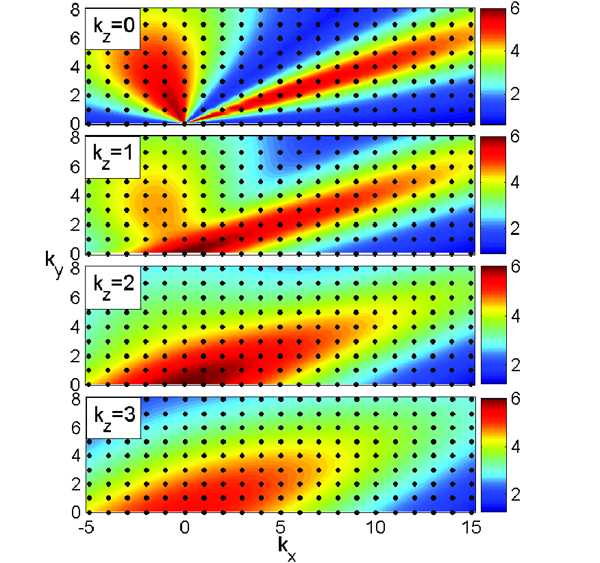
Figure 1: Map of $G$ in $(k_{x},k_{y})$-plane at $t_{d}=1.33$ and various $k_{z}=0,1,2,3$ calculated with the linearized version of the main Equations (A1)-(A9). The black dots represent discrete modes in the box. It is seen that the vital area (red and yellow), where the largest nonmodal growth occurs, is sufficiently densely populated with these modes.

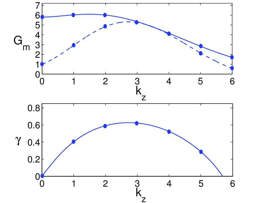
Figure 2: The upper panel shows the nonmodal growth factor, $G_{m}$ (solid line), of the axisymmetric and radially uniform ($k_{x}=k_{y}=0$) modes vs. $k_{z}$ at $t_{d}=1.33$ together with the modal growth factor of the energy, $\exp(2\gamma t_{d})$ (dashed line), of these modes for the same time. Here $\gamma$ is the corresponding modal (exponential) growth rate at $k_{x}=k_{y}=0$ and the same values of $\beta,{\rm Re},{\rm Rm}$, which is plotted in the lower panel vs. $k_{z}$. In both panels, $k_{z}$ is in units of $2\pi$ and dots indicate the growth factors and growth rate at discrete $k_{z}=1,2,3,...$ present in the box.

We quantify the nonmodal growth of individual modes in terms of the maximum possible, or optimal growth factor, $G$, of the total spectral energy, ${\cal E}$, by a specific time $t_{d}$, which was used in Squire & Bhattacharjee (2014) and Paper I. The reference time, $t_{d}$, is usually of the order of the orbital time. For definiteness, here we take it as the $e$-folding time of the most unstable MRI channel mode in the ideal case, $t_{d}=1/\gamma_{max}=1.33$ (in units of $\Omega^{-1}$), where $\gamma_{max}=0.75\Omega$ is its growth rate (Balbus & Hawley, 1991), because this time is also of the order of the dynamical time.

Figure 1 presents the growth factor $G$ at different vertical wavenumbers $k_{z}=0,1,2,3$. It is plotted as a function of the wavenumber $k_{x}(t_{d})=k_{x}(0)+qk_{y}t_{d}$, which an optimal mode with initial radial $k_{x}(0)$ and azimuthal $k_{y}$ wavenumbers has at time $t_{d}$ as a result of drift due to the shear. Although the maximum of the nonmodal amplification in $(k_{x},k_{y})$-plane, $G_{m}$, at fixed $k_{z}$, comes at axisymmetric modes with $k_{x}=k_{y}=0$, there is a broad range of non-axisymmetric modes achieving comparable growth (red and yellow areas). At $k_{z}=0$, the linear magnetic and velocity perturbations are decoupled: there are two separate amplification regions, the right corresponding to magnetic perturbations and the left to kinetic ones, both with growth factors smaller than that at $k_{z}=1$. The maximum nonmodal growth $G_{m}$ vs $k_{z}$ is shown in Figure 2. For the sake of comparison, this figure also shows the modal (exponential) growth rate, $\gamma$, of these horizontally uniform $k_{z}=k_{y}=0$ modes, which are known to exhibit the fastest growth also in the modal theory of MRI (e.g., Pessah & Chan, 2008), and the corresponding modal growth factor at $t_{d}$, $\exp(2\gamma t_{d})$, as a function of $k_{z}$ for the same values of $\beta,{\rm Re},{\rm Rm}$. It is evident that the nonmodal and modal growths exhibit different dependencies on $k_{z}$: $G_{m}$ achieves a maximum at around $k_{z}=1$ and decreases with increasing $k_{z}$, whereas $\gamma$ and the associated modal growth factor reaches a maximum near $k_{z}=3$ and decrease at small and large $k_{z}$. Note also in the upper panel of Figure 2 that the nonmodal growth is larger than or equal to the modal one at all $k_{z}$, especially at the dynamically active small $k_{z}=0,1$. We will see below that the axisymmetric mode $k_{x}=k_{y}=0,k_{z}=1$, which undergoes higher nonmodal amplification and is referred to as the channel mode, is in fact the most active participant in the nonlinear (turbulence) dynamics as well. Of course, in the turbulent state, the nonlinear terms qualitatively modify the dynamical picture, resulting in somewhat different behavior with $k_{z}$ (see e.g., Figure 4), still the linear analysis presented here gives a preliminary feeling/insight into energy exchange process with the basic flow and, most importantly, vividly shows substantial influence of the disk flow nonnormality on the growth factors of spectrally/modally unstable modes.

We stress that the nonmodal growth phenomenon – mathematically the nonnormality (non-self-adjointness) of linear evolution operators – is inherently caused by shear and, according to the above calculations, is significant for both non-axisymmetric and axisymmetric (channel) modes in MRI-active disks with a net vertical field. Specifically, the channel modes, which are stronger in this case, grow purely exponentially only at large times, whereas their growth during finite/dynamical time is governed by nonmodal physics and can have growth factors larger than the modal one during these times (Figure 2). In the case of (net vertical field) MRI-turbulence, the characteristic timescales of dynamical processes are evidently of the order of orbital/shear time (Walker et al., 2016). Therefore, it is necessary to take into account nonmodal effects on the channel mode dynamics and not rely solely on its modal growth in order to properly understand saturation and energy balance processes of the turbulence. (This point regarding the importance of nonmodal physics in the dynamics of (axisymmetric) modes in MRI-turbulence was also emphasized by Squire & Bhattacharjee (2014)). Thus, for a full representation of the dynamical picture, it is important that a simulation box sufficiently well encompasses these nonmodally most amplified modes. The discrete modes contained in the adopted box $(4,4,1)$ are shown as black dots on the map of $G$ in Figure 1. It is seen that they indeed sufficiently densely cover the yellow and red regions of the largest nonmodal amplification, which, in turn, justifies its choice in the present study.

Table 1: Simulation parameters: box size, number of grid points, stratification and the Reynolds number. In all the runs, ${\rm Rm}={\rm Pe}={\rm Re}$ and $N^{2}=0.25$, except for the unstratified run, where $N^{2}=0$ and accordingly ${\rm Pe}$ is absent.

$(L_{x},L_{y},L_{z})$	$(N_{x},N_{y},N_{z})$	stratification	${\rm Re}$
$(4,4,1)$	$(256,256,128)$	yes	3000
$(4,4,1)$	$(256,256,128)$	no	3000
$(4,4,1)$	$(256,256,128)$	yes	6000

Thus, the above-presented linear nonmodal stability analysis allows us to optimize the simulation parameters for the nonlinear (turbulent) regime, especially, the domain size such as to include as fully as possible the dynamics of essential active modes defining MRI-turbulence dynamics. In addition to the fiducial run described above, we performed two other simulations with the same box aspect ratio (Table I), the first of which is carried out in the unstratified case in order to compare with the fiducial stratified case and the second one is to confirm that increasing Reynolds number does not change a qualitative picture of the dynamical processes. The analysis presented in the following sections is based on the fiducial model and it is stated explicitly wherever the results from other runs appear.

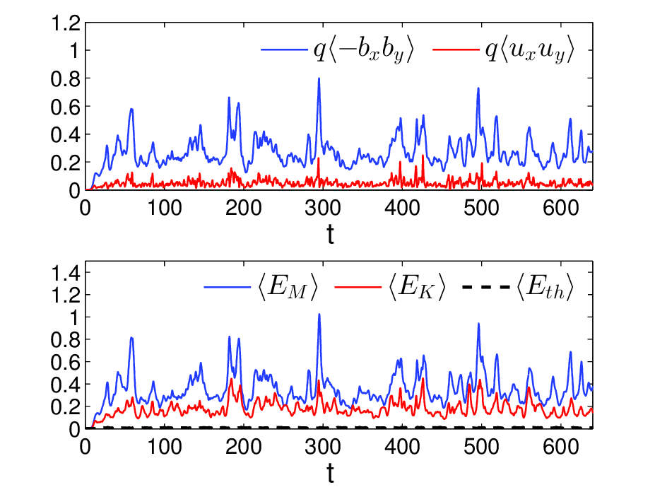
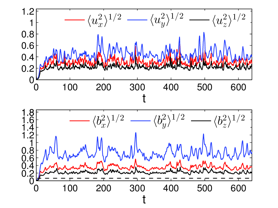
Figure 3: Volume-averaged stresses (top row), energy densities (second row) and the rms of velocity (third row) and magnetic field (bottom row) components as a function of time. These quantities are characterized by recurrent bursts all along the evolution, as is characteristic for vertical field MRI-turbulence. Magnetic energy is on average about twice larger than the kinetic one, while the thermal energy is relatively small. The Maxwell stress is larger than the Reynolds one on average by a factor of 5.5. The azimuthal components of the turbulent velocity and magnetic field exhibit more pronounced bursts with higher peaks than those for the respective other two components. For reference, dashed line in the bottom panel corresponds to the background vertical field $B_{0z}=0.0447$.

4 Numerical simulations and characteristic features of the turbulence

Initial perturbations grow mainly due to the nonmodal mechanism, which later continues into exponential growth for axisymmetric modes. After a few orbits, the flow breaks down into a fully developed MHD turbulence. Figure 3 shows the evolution of the volume-averaged perturbed kinetic and magnetic quantities in the turbulent state. The magnetic energy is on average larger than the kinetic one by a factor of about 2 and both dominate the thermal energy. The Maxwell stress exceeds the Reynolds one on average by a factor of about 5.5. The azimuthal components of the velocity and magnetic field are always larger than the other two respective ones due to the shear; the imposed vertical field is dominated by the turbulent magnetic field with the time-averaged rms values $\langle b_{x}^{2}\rangle^{1/2}=8B_{0z}$, $\langle b_{y}^{2}\rangle^{1/2}=16B_{0z}$, $\langle b_{z}^{2}\rangle^{1/2}=4.9B_{0z}$. As seen in Figure 3, the main characteristic feature of the temporal evolution of all these quantities, which distinguishes the vertical field case from the azimuthal one analyzed in Paper I, is a burst-like behavior with intermittent peaks and quiescent intervals, as also observed in other related studies on net vertical field MRI-turbulence (e.g., Sano & Inutsuka, 2001; Lesur & Longaretti, 2007; Bodo et al., 2008; Longaretti & Lesur, 2010; Murphy & Pessah, 2015). The peaks are most pronounced/intensive in the azimuthal velocity and magnetic field, inducing corresponding peaks in the magnetic energy and Maxwell stress. As a result, these bursts yield enhanced rates of angular momentum transport. On a closer examination, one can notice that the peaks in the rms of $u_{z}$ and $b_{z}$ follow just after the respective stronger peaks in the rms of $u_{y}$ and $b_{y}$ (see also Murphy & Pessah, 2015). We show below that these bursts are in fact closely related to the manifestations of the dynamics of two modes:
– the channel mode with wavenumber ${\bf k}_{c}=(0,0,\pm 1)$, which is horizontally uniform varying only on the largest $z$-vertical scale in the box, and
– the zonal flow mode with wavenumber ${\bf k}_{zf}=(\pm 1,0,0)$ varying only on the largest $x$-radial scale in the box.
Namely, the burst-like growth of the channel mode due to MRI amplifies $x$- and, especially, $y$-components of velocity and magnetic field (the channel mode itself does not possess the $z$-components of these quantities). In turn, its nonlinear interaction with other dynamically active non-axisymmetric modes (referred to as parasitic modes in the literature) shortly afterwards gives rise to the peaks of the $z$-components of these quantities. Below we show that this nonlinear interaction is mainly manifested as the transverse cascade in ${\bf k}$-space.

The role of the channel mode and hence the intensity of bursts depend on the box aspect ratio $L_{x}/L_{z}$, being more pronounced when this aspect ratio is around unity, but becoming weaker as it increases (Bodo et al., 2008). However, as we demonstrate in this paper, the channel mode is a key participant in the dynamics of a net vertical field MRI-turbulence. In particular, the adopted here box $(4,4,1)$ would exhibit only relatively weak bursts according to Bodo et al. (2008), while as we found here, the amplification of the channel mode can nevertheless influence the behavior of other active modes and ultimately the total stress and energy.

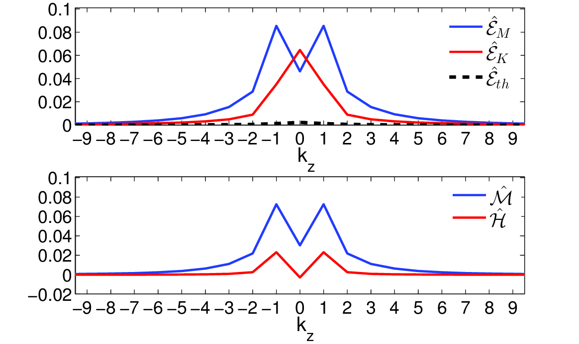
Figure 4: Integrated in $(k_{x},k_{y})$-plane time-averaged 1D spectral energies and stresses as a function of $k_{z}$.

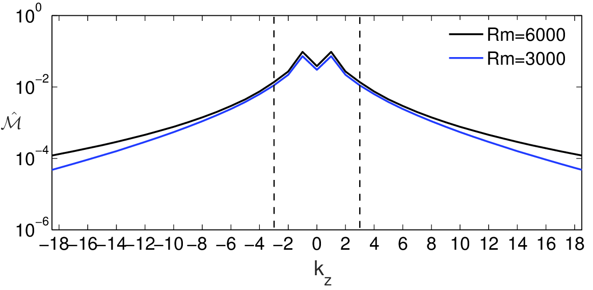
Figure 5: $\hat{\cal M}$ vs. $k_{z}$ at ${\rm Re}={\rm Rm}=3000$ (blue) for the fiducial model (from Figure 4) and at ${\rm Re}={\rm Rm}=6000$ (black). The vital area along $k_{z}$-axis lies within the vertical dashed lines. It is seen that the difference between the lower and higher ${\rm Rm}$ cases are noticeable only at larger $|k_{z}|$ outside the vital area, leaving the main dynamical processes within the vital area at small $|k_{z}|$ nearly unaffected.

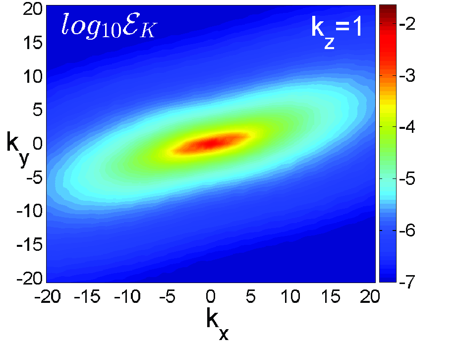
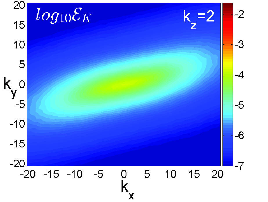
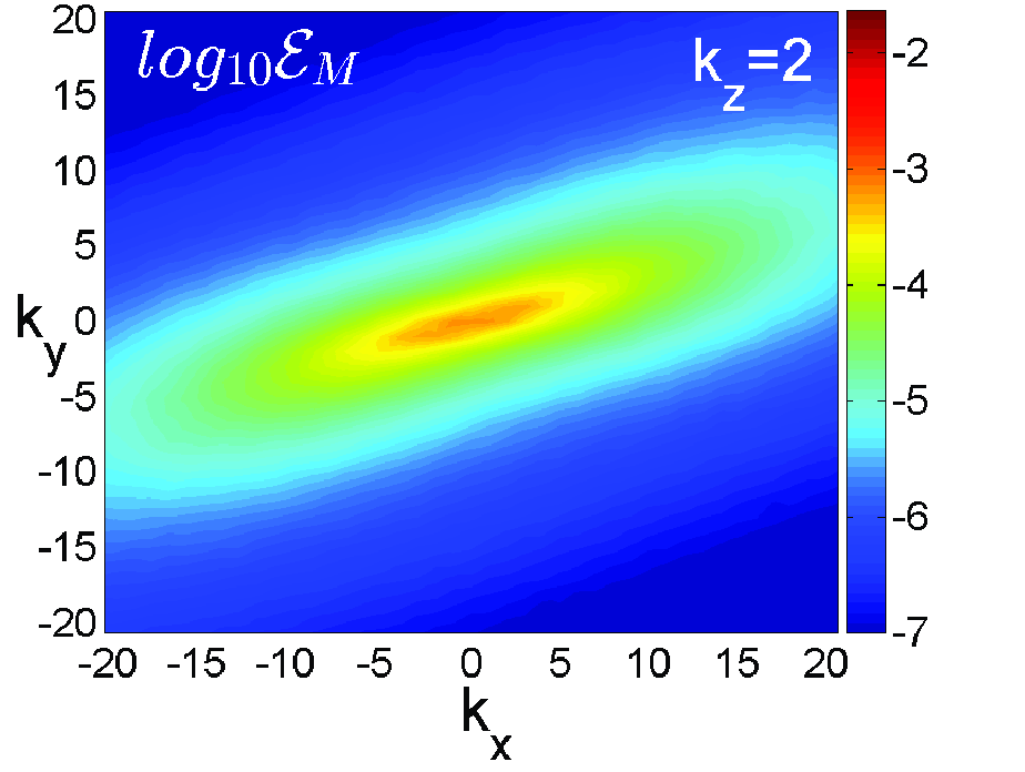
Figure 6: Slices of the time-averaged logarithmic 3D spectra of the kinetic, $log_{10}{\cal E}_{K}$ (upper row), and magnetic, $log_{10}{\cal E}_{M}$ (lower row), energies in $(k_{x},k_{y})$-plane at $k_{z}=0,1,2$. Both spectra are strongly anisotropic with similar overall shape and inclination towards $k_{x}$-axis. The maximum of the kinetic energy spectrum comes at the zonal flow mode ${\bf k}_{zf}=(\pm 1,0,0)$, while that of the magnetic energy spectrum at the channel mode ${\bf k}_{c}=(0,0,\pm 1)$.

4.1 Energy spectra

We start the analysis of the 3D spectra of the energies by examining first their dependence on the vertical wavenumber. For this purpose, we integrate the spectra of the energies and the stresses in $(k_{x},k_{y})$-plane, $\hat{\cal E}_{K,M,th}(k_{z})=\int{\cal E}_{K,M,th}dk_{x}dk_{y}$, $(\hat{\cal H}(k_{z}),\hat{\cal M}(k_{z}))=\int({\cal H},{\cal M})dk_{x}dk_{y}$, then average over time from $t=100$ till $t=650$ and represent as a function of $k_{z}$ in Figure 4. The spectral magnetic energy is larger than the kinetic one except at $k_{z}=0$, where they are comparable, and both dominate the spectral thermal energy; the spectral Maxwell stress, in turn, is higher than the Reynolds one. The maximum of the magnetic energy as well as both stresses comes at $|k_{z}|=1$, corresponding to the channel mode ${\bf k}_{c}=(0,0,\rm 1)$. Thus, most of energy supply by the stresses occurs in fact at $|k_{z}|=0,1,2$ rather than at $|k_{z}|=3$ that corresponds to the most unstable axisymmetric mode of MRI in the modal approach for our parameters (lower panel of Figure 2). This is in agreement with the above linear nonmodal analysis, which have demonstrated how the nonnormality eliminates the dominance of the $|k_{z}|=3$ mode in preference to lower $k_{z}$ modes during finite times (Figures 1 and 2). This result supports again the statement made above that the nonmodal growth over short, dynamical/orbital timescale is more relevant in the turbulent state. A maximum of the kinetic energy spectrum is instead at $k_{z}=0$ and is a bit higher than the magnetic energy at this $k_{z}$. It corresponds to the axisymmetric zonal flow mode with ${\bf k}_{zf}=(\pm 1,0,0)$.

The main energy-carrying dynamical processes concentrated mostly at small $|k_{z}|=0,1,2$ in the vital area are nearly unaffected by dissipation, as demonstrated in Figure 5 showing the 1D spectra of the Maxwell stress, $\hat{\cal M}$, for the fiducial run and at twice higher Reynolds numbers. The difference between these two spectra is only appreciable outside the vital area, where the stress as well as the energies fall off by about three orders of magnitude and therefore these wavenumbers are not anyway dynamically important.

Having examined the dependence of the spectra on the vertical wavenumber, we now present in Figure 6 slices of the 3D spectra of the kinetic, ${\cal E}_{K}$, and magnetic, ${\cal E}_{M}$, energies in $(k_{x},k_{y})$-plane. Both spectra are fairly anisotropic due to the shear with a similar overall elliptical form. We checked that this spectral anisotropy in fact extends to larger wavenumbers, up to the dissipation scale. The maximum of the kinetic energy spectrum comes at the wavenumber ${\bf k}_{zf}=(\pm 1,0,0)$ of the zonal flow mode, while the maximum of the magnetic energy spectrum comes at the channel mode wavenumber ${\bf k}_{c}=(0,0,\pm 1)$. These spectra also indicate that there is a broad range of trailing non-axisymmetric modes (red areas) with energies, on average, comparable to that of the channel mode and hence taking an active part in the turbulence dynamics (see also Longaretti & Lesur, 2010). By contrast, in the case with azimuthal field in Paper I, although the maximum of the magnetic energy spectrum comes again at $k_{z}=1$, in the $(k_{x},k_{y})$-plane, this maximum comes instead at nearby non-axisymmetric modes with $|k_{y}|=1$, while the channel mode is not dynamically as significant. A more detailed analysis of the relative roles and dynamics of the channel, zonal flow and other (non-axisymmetric) modes is presented below. Although not shown here, the slices of the 3D spectrum of the Maxwell stress in $(k_{x},k_{y})$-plane share a similar shape and type of anisotropy as the magnetic energy spectrum in Figure 6. Finally, we note that analogous anisotropic energy spectra were also observed in other local studies of MRI-turbulence with a nonzero net vertical field (Hawley et al., 1995; Lesur & Longaretti, 2011; Murphy & Pessah, 2015).

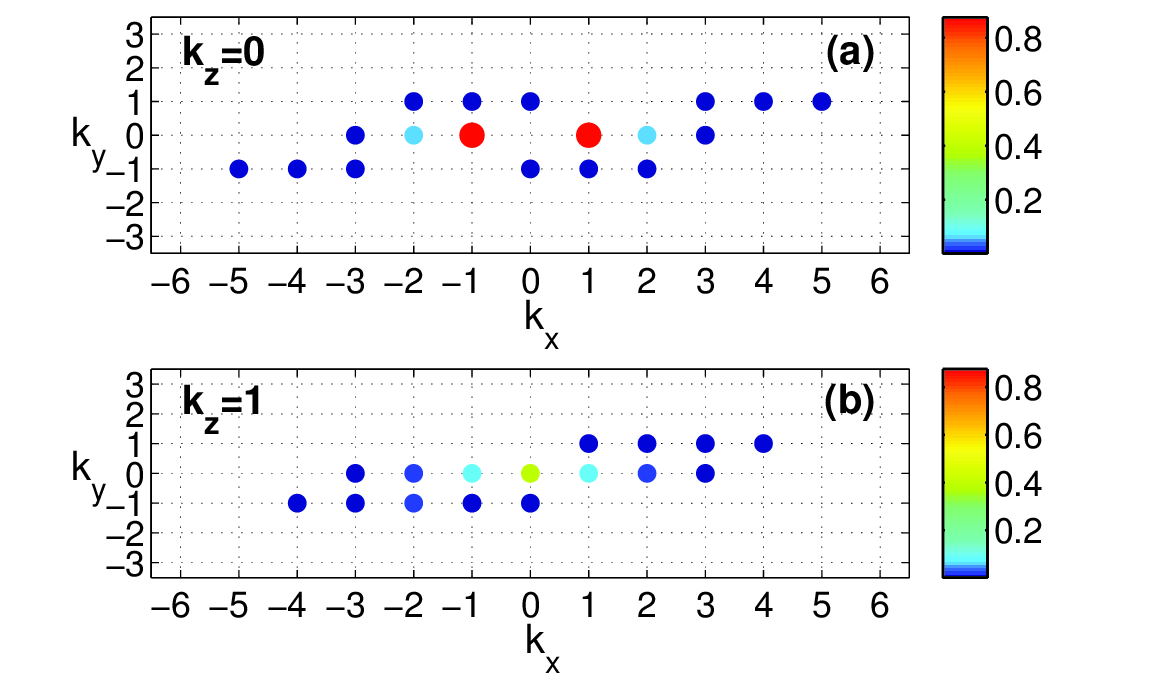
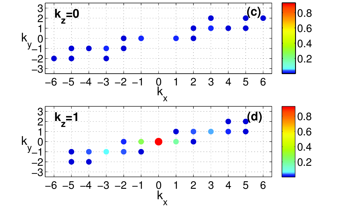
Figure 7: Active modes (color dots) in k-space at $k_{z}=0,1$, as defined in the text, computed separately for the kinetic [panels (a) and (b)] and magnetic [panels (c) and (d)] components. The mode colors denote the time, relative to the entire duration of the run, during which each of these modes retains energy higher than 50 % of the maximum spectral energy. The zonal flow mode ${\bf k}_{zf}=(\pm 1,0,0)$ and the channel mode ${\bf k}_{c}=(0,0,\pm 1)$ [denoted by bigger red dots, respectively, in panels (a) and (d)] clearly stand out against other modes, as they retain, respectively, higher kinetic and magnetic energies most of the time.

4.2 Active modes in ${\bf k}$-space

The dynamically important modes with most effective amplification have been identified above based on the optimal nonmodal growth calculations (Figure 1), i.e., on the analysis of the linear dynamics. However, the overall dynamical picture of the turbulence is formed as a result of the interplay of linear and nonlinear processes. So, it is reasonable to introduce the notion of active modes in k-space – the energy-carrying modes playing a major role in the dynamics – separately for the kinetic and magnetic components. The active kinetic (magnetic) modes are labeled those modes whose spectral kinetic (magnetic) energy is higher than $50\%$ of the maximum spectral kinetic energy ${\cal E}_{K,max}$ (magnetic energy ${\cal E}_{M,max}$) at the same time. Both types of active modes in Fourier space at $k_{z}=0,1$ are shown in Figure 7 with color dots. The color of each mode indicates the fraction of the total evolution time during which this mode retains the higher energy. These dynamically active modes are located anisotropically in $(k_{x},k_{y})$-plane in the region of wavenumbers, $|k_{x}|\leq 6,|k_{y}|\leq 2$, forming the so-called vital area of the turbulence in k-space. In this area, the most energetic dynamical processes are concentrated that set the strength and statistical properties of the turbulence. There are two – the channel ${\bf k}_{c}$ and the zonal flow ${\bf k}_{zf}$ – modes (bigger red dots, respectively, in panels (a) and (d) of Figure 7) that clearly stand out against other modes, as they retain, respectively, higher magnetic (the channel mode) and kinetic (the zonal flow mode) energies most of the time. As a result, these two modes play a key role in shaping the turbulence dynamics and deserve a more detailed analysis, which is given in the following subsections.

Apart from the channel and zonal flow modes, there are a sufficient number of other active modes (blue dots in Figure 7) that individually are not so significant compared to these two modes, since they retain the higher kinetic or magnetic energies for much less a time. However, the combined action of the multitude of these modes is competitive to the channel and zonal flow modes. We label them as the rest modes and describe in a devoted subsection 4.5 below. By contrast, in the case of a purely azimuthal field (Paper I), these rest non-axisymmetric modes (mainly those with $|k_{y}|=1$ and $k_{z}=0,1$) prevail not only collectively but also individually – they carry energies higher or comparable to that of the channel mode for longer times than those in the present case with net vertical field. This results in different properties of the turbulence defined instead by dominant individual non-axisymmetric rest modes. The other modes (including those with $|k_{z}|\geq 2$ not shown in Figure 7) lie outside the vital area, playing only a minor role in the dynamics

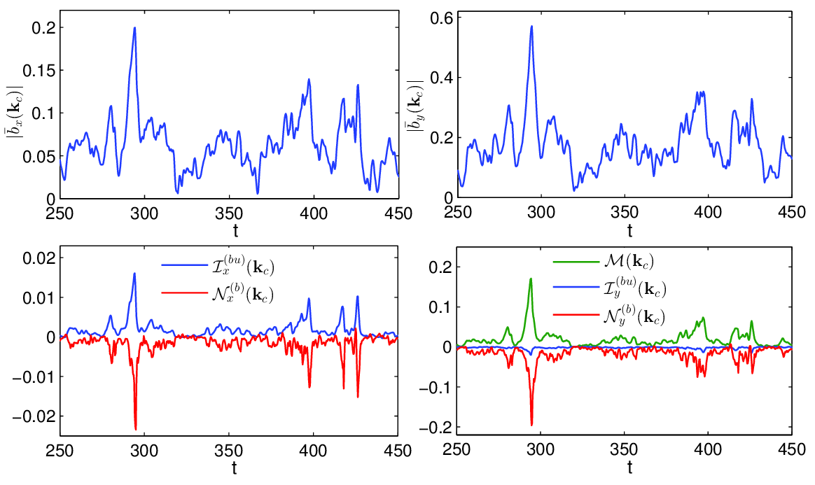
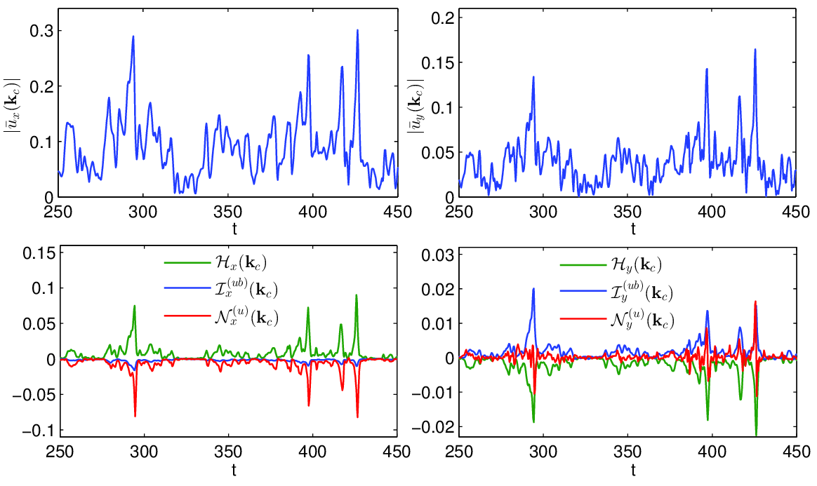
Figure 8: Evolution of the main spectral amplitudes of the magnetic field, $|\bar{b}_{x}({\bf k}_{c})|,|\bar{b}_{y}({\bf k}_{c})|$, and velocity, $|\bar{u}_{x}({\bf k}_{c})|,~{}|\bar{u}_{y}({\bf k}_{c})|$, of the channel mode with ${\bf k}_{c}=(0,0,\pm 1)$ as well as the corresponding time-histories of the linear – stresses, ${\cal M}({\bf k}_{c})$, ${\cal H}({\bf k}_{c})$, and exchange, ${\cal I}^{(ub)}({\bf k}_{c})$, ${\cal I}^{(bu)}({\bf k}_{c})$ – and nonlinear, ${\cal N}^{(u)}({\bf k}_{c})$, ${\cal N}^{(b)}({\bf k}_{c})$, terms, which govern the dynamics of this mode. The channel mode is supported by the linear processes – the action of the stresses and the linear exchange terms describe its amplification due to MRI, while the nonlinear terms mostly oppose this growth, resulting in the recurrent bursts in the evolution of the magnetic field and velocity. $|\bar{b}_{x}|$ and $|\bar{b}_{y}|$ are amplified, respectively, by ${\cal I}_{x}^{(bu)}$ and ${\cal M}$, as they are always positive, and then drained, respectively, by the nonlinear terms ${\cal N}_{x}^{(b)}$ and ${\cal N}_{y}^{(b)}$, which are always negative, transferring energy to other wavenumbers and components (see Figures 12 and 14). Consequently, the negative peaks of these terms a bit lag the corresponding peaks of the linear terms. This azimuthal field component is also drained to a lesser degree by ${\cal I}_{y}^{(bu)}$, giving its energy to $|\bar{u}_{y}|$. $|\bar{u}_{x}|$ is amplified by positive ${\cal H}_{x}$ and drained by negative ${\cal N}_{x}^{(u)}$ and, to a lesser degree, by ${\cal I}_{x}^{(ub)}$ – the peaks of the latter two sink terms lag those of the linear source term ${\cal H}_{x}$. $|\bar{u}_{y}|$ is amplified by ${\cal I}_{y}^{(ub)}$ and drained by always negative ${\cal H}_{y}$. ${\cal N}_{y}^{(u)}$ alternates sign, as distinct from the other nonlinear terms, providing for $|\bar{u}_{y}|$ either source, when positive, or sink, when negative. The influence of the nonlinear terms is maximal at the peaks of $|\bar{b}_{x}({\bf k}_{c})|$ and $|\bar{b}_{y}({\bf k}_{c})|$ – they halt the MRI-growth and lead to a fast drain of the channel mode over a few orbital periods.

4.3 The channel mode

We have seen above that the channel mode – the harmonic with wavenumber ${\bf k}_{c}=(0,0,\pm 1)$ that is uniform in the horizontal $(x,y)$-plane and has the largest vertical wavelength (correspondingly, the smallest wavenumber, $k_{z}=\pm 1$) in the domain – is a key participant in the turbulence dynamics. It carries higher energy most of the time in the turbulent state among other active modes in the vital area and corresponds to the maximum of the spectral magnetic energy and stresses in Fourier space at any moment (see Figure 10 below). So, first we analyze the dynamics of this mode and then move to the zonal flow and the rest modes.

Figure 8 shows the evolution of the main spectral amplitudes of the magnetic field, $|\bar{b}_{x}({\bf k}_{c})|,|\bar{b}_{y}({\bf k}_{c})|$, and velocity, $|\bar{u}_{x}({\bf k}_{c})|,~{}|\bar{u}_{y}({\bf k}_{c})|$ of the channel mode. Also plotted are the time-histories of the corresponding linear – stresses, ${\cal M}({\bf k}_{c})$, ${\cal H}({\bf k}_{c})$ and exchange ${\cal I}^{(ub)}({\bf k}_{c})$, ${\cal I}^{(bu)}({\bf k}_{c})$ – and nonlinear, ${\cal N}^{(u)}({\bf k}_{c})$, ${\cal N}^{(b)}({\bf k}_{c})$, terms in the above spectral Equations (7)-(8) and (21)-(22), which govern the dynamics of this mode. The action of the stresses and exchange terms describes together the (nonmodal) effect of MRI on the channel mode and are mainly responsible for its amplification. The action of the nonlinear terms describes, in turn, interaction of the channel mode with other active modes with different wavenumbers and components (this process is covered in detail in subsection 4.6, see also Figures 12 and 14 below). These linear and nonlinear terms jointly determine the temporal evolution of the channel mode’s velocity and magnetic field with characteristic recurrent bursts seen in Figure 8. It is clear from this figure that the typical variation, or dynamical time of the nonlinear terms is indeed of the order of the orbital time, indicating again that the nonmodal physics of MRI is more relevant in the state of developed turbulence. Analysis of these terms allows us to understand nuances of the channel mode dynamics and ultimately the behavior of the total stress and the energy (Figure 3), because, as we will see below (subsection 4.5), the channel mode bursts manifest themselves in the time-development of the volume-averaged magnetic energy and the Maxwell stress. These terms operate differently for velocity and magnetic fields.

Let us first consider the magnetic field components in Figure 8. $|\bar{b}_{x}|$ and $|\bar{b}_{y}|$ are amplified, respectively, by ${\cal I}_{x}^{(bu)}$ and ${\cal M}$, as they are always positive, and then drained, respectively, by the nonlinear terms ${\cal N}_{x}^{(b)}$ and ${\cal N}_{y}^{(b)}$, which are always negative, transferring energy to other wavenumbers and components. Consequently, the negative peaks of these nonlinear terms a bit lag the corresponding peaks of the linear terms. The azimuthal field, which is a dominant field component in the channel mode, is also drained to a lesser degree by the negative exchange term ${\cal I}_{y}^{(bu)}$, transferring its energy to $|\bar{u}_{y}|$. As for the velocity components, $|\bar{u}_{x}|$ is amplified by positive ${\cal H}_{x}$, then drained mostly by ${\cal N}_{x}^{(u)}$, which is always negative and, to a lesser degree, by also negative ${\cal I}_{x}^{(ub)}$ – the peaks of the latter two sink terms lag corresponding peaks of the linear source term ${\cal H}_{x}$. Finally, $|\bar{u}_{y}|$ is mostly amplified by ${\cal I}_{y}^{(ub)}$, taking energy from $|\bar{b}_{y}|$, and is drained by always negative ${\cal H}_{y}$. ${\cal N}_{y}^{(u)}$ acts differently from the above nonlinear terms – it alternates sign, providing for $|\bar{u}_{y}|$ either source, when positive, or sink, when negative. So, other modes via nonlinear interaction occasionally reinforce the growth of the channel mode’s azimuthal velocity, which is primarily due to MRI and is represented by the exchange term ${\cal I}_{y}^{(ub)}$ which is always positive.

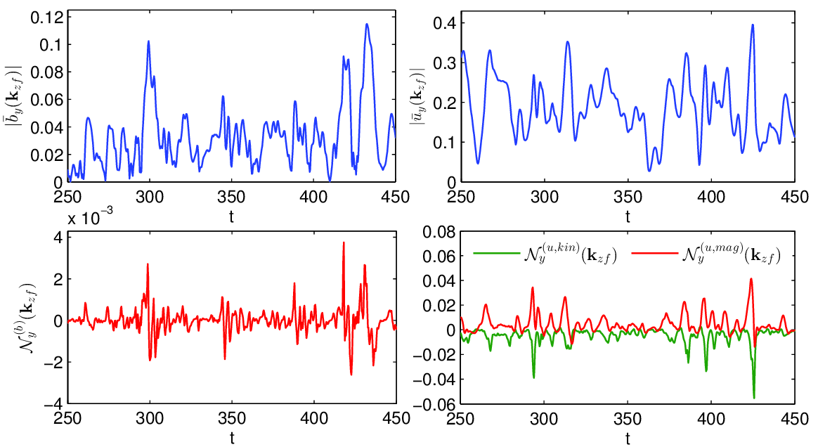
Figure 9: Evolution of the azimuthal magnetic field, $\bar{b}_{y}({\bf k}_{zf})$, and velocity, $\bar{u}_{y}({\bf k}_{zf})$, components of the zonal flow mode with ${\bf k}_{zf}=(\pm 1,0,0)$ as well as the corresponding nonlinear terms ${\cal N}_{y}^{(b)}({\bf k}_{zf})$, ${\cal N}_{y}^{(u,kin)}({\bf k}_{zf})$, ${\cal N}_{y}^{(u,mag)}({\bf k}_{zf})$, which drive this mode. The azimuthal velocity $\bar{u}_{y}$ is dominant in this mode. It is produced by the magnetic part ${\cal N}_{y}^{(u,mag)}$, as it is mostly positive, and drained by the hydrodynamic part ${\cal N}_{y}^{(u,kin)}$, which is always negative.

In conclusion, the channel mode is supported by the linear – nonmodal MRI growth – processes, while nonlinear processes mostly oppose this growth. The effect of the nonlinear terms is maximal during the peaks of $|\bar{b}_{x}({\bf k}_{c})|$ and $|\bar{b}_{y}({\bf k}_{c})|$ – they halt the growth and lead to a fast drain of the channel mode energy, redistributing this energy to other modes. Thus, in a strict self-consistent approach of the net vertical field MRI-turbulence, this redistribution of the channel mode energy to other modes is actually due to the nonlinear processes (in the form of the transverse cascade, Figures 12 and 14). However, in previous studies, the channel mode has been considered, for simplicity, not as a variable/perturbation mode itself, but as a part of the basic/stationary dynamics (see e.g., Goodman & Xu, 1994; Pessah & Goodman, 2009; Latter et al., 2009; Pessah, 2010). In those analysis, the redistribution of the channel mode energy to other modes is classified as a linear process – called parasitic instability – and these modes (parasites, in our terms “the rest modes”), which feed on the channel mode, are assumed to have smaller amplitudes than that of the latter. This simplified approach definitely gives a good feeling of the broadening of perturbation spectrum at the expense of the channel mode. At the same time, this simplification might somewhat suffer from inaccuracy when used for the turbulent case, since the channel mode in fact is not stationary and consists of a chaotically repeated processes of bursts and subsequent drains – chaotic are both the values of the peaks as well as time intervals between them.

4.4 The zonal flow mode

The second mode that also plays an important role in the turbulence dynamics is the zonal flow mode – the harmonic with wavenumber ${\bf k}_{zf}=(\pm 1,0,0)$ that is independent of the azimuthal and vertical coordinates (i.e., is axisymmetric and vertically uniform) and has the largest radial wavelength (correspondingly, the smallest wavenumber, $k_{x}=\pm 1$) in the domain. Zonal flow in MRI-turbulence with zero and nonzero net vertical field was found in several studies Johansen et al. (2009); Bai & Stone (2014); Simon & Armitage (2014), however, its dynamics was usually analyzed based on the simplified models. Here we trace the zonal flow evolution in Fourier space self-consistently (without invoking the simplified models) by examining its governing dynamical terms in the main spectral equations directly from the simulation data.

We have seen in Figure 7 that in the turbulent state, the zonal flow mode carries higher kinetic energy among other active modes and corresponds to the maximum of the spectral kinetic energy in Fourier space most of the evolution time (see Figure 10 below). However, this mode does not contribute to the spectral Reynolds and Maxwell stresses, because its radial velocity and magnetic field components are identically zero, $\bar{u}_{x}({\bf k}_{zf})=\bar{b}_{x}({\bf k}_{zf})=0$, due to incompressibility (A17) and divergence-free (A18) conditions. Besides, we checked that the vertical velocity, $\bar{u}_{z}({\bf k}_{zf})$, and magnetic field, $\bar{b}_{z}({\bf k}_{zf})$, components are also much smaller than the respective azimuthal ones. So, in Figure 9 we present only the evolution of the dominant spectral amplitudes of the azimuthal magnetic field, $|\bar{b}_{y}({\bf k}_{zf})|$, and velocity, $|\bar{u}_{y}({\bf k}_{zf})|$, in this mode. $|u_{y}({\bf k}_{zf})|$ changes on longer timescale corresponding to axisymmetric zonal flow in physical space, while $|b_{y}({\bf k}_{zf})|$ together with longer also exhibits shorter timescale variations. It is readily seen that the linear – stresses and exchange – terms are identically zero for the zonal flow mode in Equations (8) and (22), ${\cal H}_{y}({\bf k}_{zf})={\cal M}({\bf k}_{zf})=0$, ${\cal I}_{y}^{(ub)}({\bf k}_{zf})={\cal I}_{y}^{(u\theta)}({\bf k}_{zf})=0$. Thus, the linear processes (i.e., MRI) do not affect this mode. Therefore, it can be supported only by the nonlinear terms ${\cal N}_{y}^{(u)},{\cal N}_{y}^{(b)}$. Since $\bar{u}_{y}$ is the dominant component in this mode, we look more into its nonlinear term in order to pin down a mechanism of zonal flow generation. This term consists of the magnetic, ${\cal N}^{(u,mag)}_{y}$, and hydrodynamic, ${\cal N}^{(u,kin)}_{y}$, contributions,

$${\cal N}^{(u)}_{y}={\cal N}^{(u,mag)}_{y}+{\cal N}^{(u,kin)}_{y},$$ (33)

which for ${\bf k}_{zf}=(\pm 1,0,0)$, have the following forms:

$${\cal N}^{(u,mag)}_{y}({\bf k}_{zf})\\ =\frac{\rm i}{2}\bar{u}^{\ast}_{y}({\bf k}_{zf})\int d^{3}{\bf k^{\prime}}\bar{b}_{y}({\bf k^{\prime}})\bar{b}_{x}({\bf k}_{zf}-{\bf k^{\prime}})+c.c.,$$ (34)

with the integrand composed of the turbulent magnetic stresses and

$${\cal N}^{(u,kin)}_{y}({\bf k}_{zf})\\ =-\frac{\rm i}{2}\bar{u}^{\ast}_{y}({\bf k}_{zf})\int d^{3}{\bf k^{\prime}}\bar{u}_{y}({\bf k^{\prime}})\bar{u}_{x}({\bf k}_{zf}-{\bf k^{\prime}})+c.c.,$$ (35)

with the integrand composed of the turbulent hydrodynamic stresses. The time-histories of these hydrodynamic and magnetic nonlinear parts as well as ${\cal N}_{y}^{(b)}$ for the zonal flow mode are also shown in Figure 9. It is seen that ${\cal N}_{y}^{(b)}({\bf k}_{zf})$ changes sign, acting as a source for $|\bar{b}_{y}({\bf k}_{zf})|$, when positive, and as a sink, when negative. On the other hand, the magnetic part is positive most of the time, producing and amplifying $|\bar{u}_{y}({\bf k}_{zf})|$. Thus, the zonal flow mode is supported by ${\cal N}^{(u,mag)}_{y}$, which describes the action of the total azimuthal magnetic tension exerted by all the rest modes on this mode. By contrast, the hydrodynamic part ${\cal N}^{(u,kin)}_{y}({\bf k}_{zf})$, which describes the total azimuthal hydrodynamic tension exerted by all other modes, is always negative and drains $|\bar{u}_{y}({\bf k}_{zf})|$. As a result, the peaks of the hydrodynamic part ${\cal N}^{(u,kin)}_{y}$ a bit lag the peaks of the magnetic part ${\cal N}^{(u,mag)}_{y}$, which initiates the growth of the azimuthal velocity.

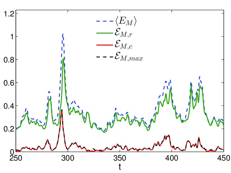
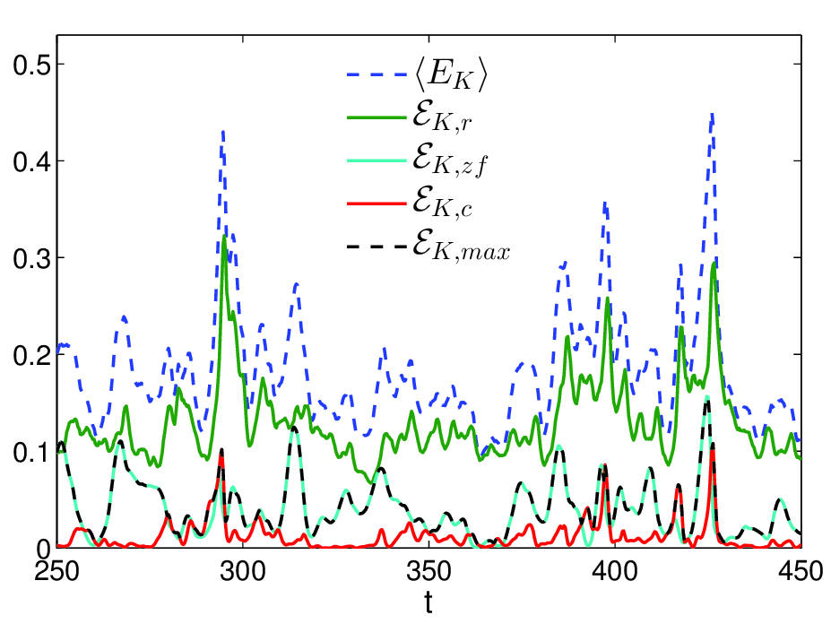
Figure 10: The left panel shows the evolution of the total magnetic energy, $\langle E_{M}\rangle$ (dashed blue), the magnetic energy of the channel mode, ${\cal E}_{M,c}$ (red), the total magnetic energy of the rest modes, ${\cal E}_{M,r}\approx\langle E_{M}\rangle-{\cal E}_{M,c}$ (green) and the maximum value of the spectral magnetic energy, ${\cal E}_{M,max}$ (dashed black), which always coincides with the energy of the channel mode. The right panel shows the evolution of the total kinetic energy, $\langle E_{K}\rangle$ (dashed blue), the kinetic energy of the channel mode, ${\cal E}_{K,c}$ (red), and of the zonal flow mode, ${\cal E}_{K,zf}$ (cyan) the total kinetic energy of the rest modes, ${\cal E}_{K,r}\approx\langle E_{K}\rangle-{\cal E}_{K,c}-{\cal E}_{K,zf}$ (green) and the maximum value of the spectral kinetic energy, ${\cal E}_{K,max}$ (dashed black), which always coincides with either the kinetic energy of the channel mode or the zonal flow mode, whichever is larger at a given time. It is also seen that the peaks of the magnetic (kinetic) energy of the rest modes tend to mainly follow the respective peaks of the magnetic (kinetic) energy of the channel mode, because, this mode nonlinearly transfers energy to the rest modes (Figure 12), causing their subsequent amplification (peak). Note also that often the zonal flow energy increases when the channel mode energy decreases and vice versa.

4.5 The rest modes

So far we have described two – the channel and zonal flow – modes that are the main participants of the dynamical processes. In addition to these modes, as classified in subsection 4.2, there are a sufficient number of active modes in the system (blue dots in Figure 7), which are not individually significant, but collectively have sufficiently large kinetic and magnetic energies - more than channel or/and zonal flow modes. Consequently, the combined influence of these modes on the overall dynamics of the turbulence becomes important. This set of active modes has been labeled as the rest modes, which, as mentioned above, are also called parasitic modes in the studies of net vertical field MRI-turbulence. As we checked, the contribution of other larger wavenumber modes, whose kinetic (magnetic) energy always remains less than 50% of the maximum spectral kinetic (magnetic) energy, in the energy balances is small compared to that of these three main types of modes and therefore is neglected below.

Figure 10 allows us to compare the total magnetic, ${\cal E}_{M,r}$ (left panel), and kinetic, ${\cal E}_{K,r}$ (right panel), energies of the rest modes with the corresponding energies of the channel and zonal flow modes at different stages of the evolution. The magnetic energy of the zonal flow mode, ${\cal E}_{M,zf}={\cal E}_{M}(-{\bf k}_{zf})+{\cal E}_{M}({\bf k}_{zf})\approx 0$, is small compared to that of the channel and the rest modes and is not shown in the left plot. In this case, the total volume-averaged magnetic energy is approximately the sum of the magnetic energies of the channel mode, ${\cal E}_{M,c}={\cal E}_{M}(-{\bf k}_{c})+{\cal E}_{M}({\bf k}_{c})$, and the rest modes, $\langle E_{M}\rangle\approx{\cal E}_{M,c}+{\cal E}_{M,r}$ (neglecting the very small contribution from the zonal flow mode), whereas in the total kinetic energy, all the three types of modes contribute: $\langle E_{K}\rangle\approx{\cal E}_{K,c}+{\cal E}_{K,zf}+{\cal E}_{K,r}$ with ${\cal E}_{K,c}={\cal E}_{K}(-{\bf k}_{c})+{\cal E}_{K}({\bf k}_{c})$ and ${\cal E}_{K,zf}={\cal E}_{K}(-{\bf k}_{zf})+{\cal E}_{K}({\bf k}_{zf})$ being the kinetic energies of the channel and zonal flow modes, respectively. In Figure 10, ${\cal E}_{M,max}$ and ${\cal E}_{K,max}$ are, respectively, the maximum values of the spectral magnetic and kinetic energies. The left panel shows that this maximum value of the magnetic energy falls on the channel mode, i.e., ${\cal E}_{M,max}={\cal E}_{M,c}$, during an entire course of the evolution. In other words, the channel mode is always magnetically the strongest among all the individual active rest modes (see also Longaretti & Lesur, 2010), although the total magnetic energy of the rest modes dominates the magnetic energy of the channel mode, ${\cal E}_{M,r}>{\cal E}_{M,c}$, especially in the quiescent intervals between the bursts, when the magnetic energy of the channel mode is relatively low. This trend is also seen in the transport due to these modes (see Figure 11 below) and points to the importance of the rest modes in the turbulence dynamics. Despite this dominance, however, it is seen in the left panel of Figure 10 that the peaks of the rest modes’ magnetic energy always occur shortly after the corresponding peaks of the channel mode’s magnetic energy, indicating that the former increases, or is driven by the latter (see subsection 4.6). Thus, the typical burst-like behavior of the nonzero the net vertical field MRI-turbulence is closely related to the manifestation of the channel mode dynamics.

The role of the rest modes is also seen in the evolution of the kinetic energies in the right panel of Figure 10. As is in the case of the magnetic energy, the contribution of the total kinetic energy of the rest modes, ${\cal E}_{K,r}$, in the volume-averaged total kinetic energy is always dominant. The kinetic energy of the zonal flow mode, ${\cal E}_{K,zf}$, is comparable to the kinetic energy of the rest modes only occasionally, while the contribution of the kinetic energy of the channel mode, ${\cal E}_{K,c}$, in the overall balance of the total kinetic energy is even less. However, also in this case, the maximum value of the spectral kinetic energy, ${\cal E}_{K,max}$, always coincides with either the kinetic energy of the channel mode or the zonal flow mode, whichever is larger at a given moment. Moreover, on a closer inspection of the kinetic energy curves, it appears that the peaks of the total kinetic energy of the rest modes in fact tends to mainly follow the corresponding peaks of the channel mode. Note also that often the zonal flow energy increases and has a peak when the channel mode energy decreases and has a minimum, that is, the zonal flow tends to grow when the channel mode is at its minimum and vice versa. This anti-correlation between the zonal flow and magnetic activity, which was also reported in Johansen et al. (2009), is further explored in Fourier space in the next subsection.

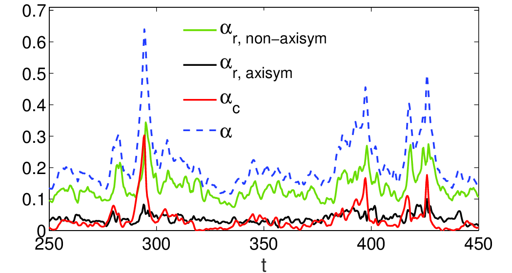
Figure 11: The transport parameter for the non-axisymmetric rest modes, $\alpha_{r,non-axisym}$ (green), for the axisymmetric rest modes, $\alpha_{r,axisym}$ (black), for the channel mode, $\alpha_{c}$ (red) and the total value $\alpha\approx\alpha_{r,non-axisym}+\alpha_{r,axisym}+\alpha_{c}$ (dashed blue). Note that the peaks in $\alpha_{r,non-axisym}$ occur shortly after the peaks of the channel mode $\alpha_{c}$, although the former dominates the latter.

Finally, we characterize the angular momentum transport due to the rest modes and compare it to that of the channel mode. The transport is measured by the normalized sum of the Maxwell and Reynolds stresses, i.e., by the usual $\alpha$ parameter which in our non-dimensional units is defined for each harmonic as,

$$\bar{\alpha}=\frac{1}{2}(\bar{u}_{x}\bar{u}_{y}^{\ast}-\bar{b}_{x}\bar{b}_{y}^{\ast})+c.c.$$

Figure 11 shows the time-histories of the transport parameter for the rest modes, separately for non-axisymmetric ones, $\alpha_{r,non-axisym}=\sum_{k_{y}\neq 0}\bar{\alpha}$ and axisymmetric ones, $\alpha_{r,axisym}=\sum_{k_{y}=0}\bar{\alpha}$, as well as for the channel mode $\alpha_{c}=\bar{\alpha}({\bf k}_{c})$ and the total transport due to all the active modes in the box, $\alpha=\sum_{\bf k}\bar{\alpha}\approx\alpha_{r,non-axisym}+\alpha_{r,axisym}+\alpha_{c}$. (The zonal flow mode does not contribute to the transport, since $\bar{u}_{x}({\bf k}_{zf})=\bar{b}_{x}({\bf k}_{zf})=0$.) Like that for the energies above, the transport due to the non-axisymmetric rest modes always dominates the transport due to the channel and axisymmetric rest modes, $\alpha_{r,non-axisym}>\alpha_{c},\alpha_{r,axisym}$. This is consistent with the results of Longaretti & Lesur (2010), who also found the prevalence of non-axisiymmetric modes over the channel mode in the transport, although they arrived on the same conclusion by calculating 1D Fourier transform of both the Maxwell and Reynolds stress as a function of $k_{y}$ at the minimum and maximum of the transport, whereas we calculate the cumulative transport of the non-axisymmetric rest modes. Note, however, that the peaks in $\alpha_{r,non-axisym}$ follow shortly after the peaks of the channel mode $\alpha_{c}$, despite the dominance of the former over the latter. At these moments, the channel mode typically exhibits more dramatic changes in the transport than the non-axiymmetric modes. This again indicates that the channel mode, nonlinearly interacting with the rest modes, acts as a trigger for the bursts in the total transport which, in turn, are primarily due to the collective activity of non-axisymmetric modes.

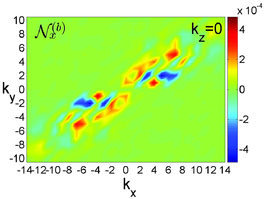
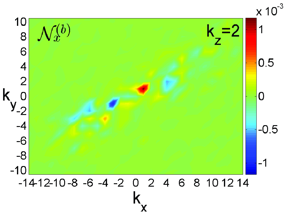
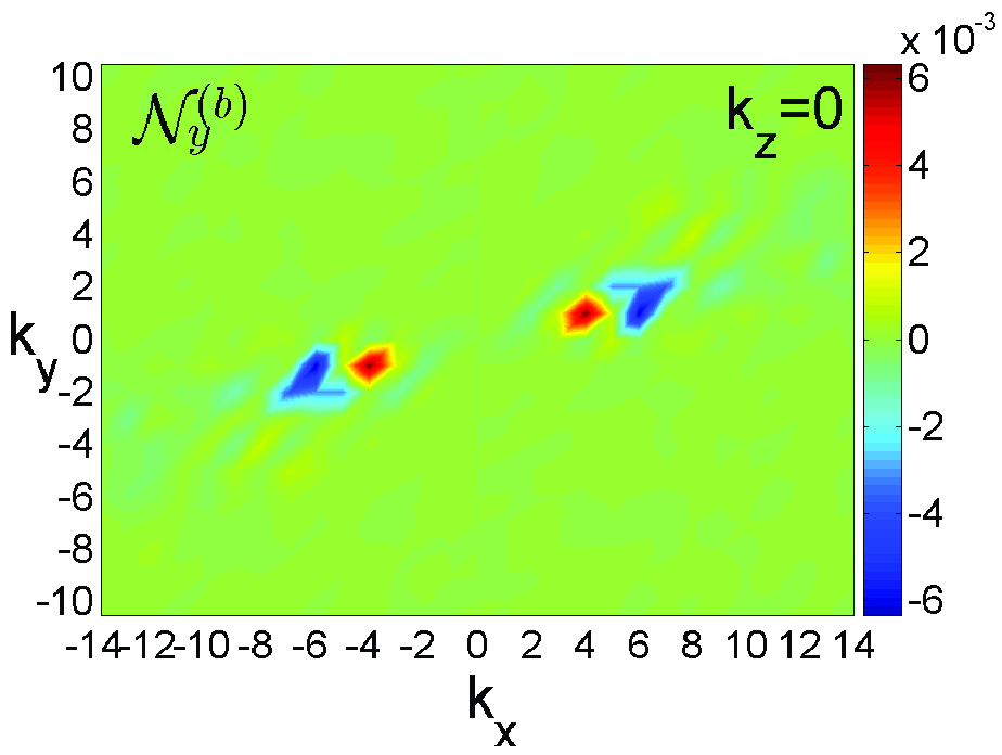
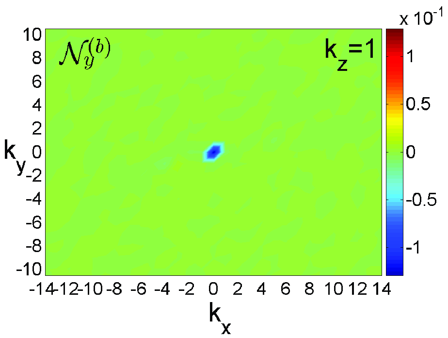
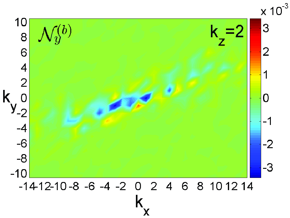
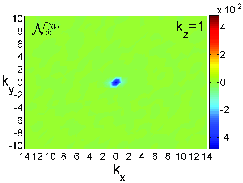
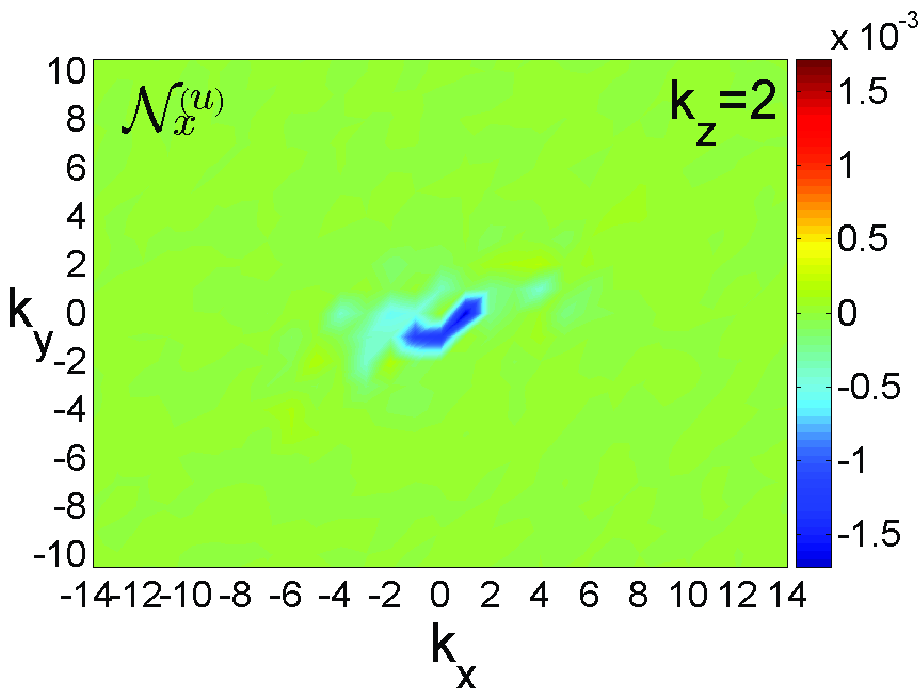
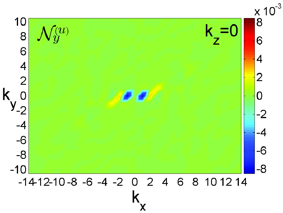
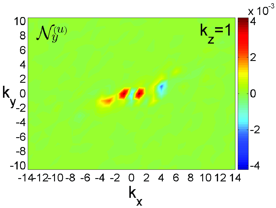
Figure 12: Spectra of the nonlinear transfer terms in $(k_{x},k_{y})$-plane at $k_{z}=0(left),1(middle),2(right)$ at around $t=294$, when the channel mode energy has a peak. At $k_{z}=1$ the nonlinear transfer terms ${\cal N}_{x}^{(b)}$, ${\cal N}_{y}^{(b)}$, ${\cal N}_{x}^{(u)}$ strongly peak near $k_{x}=k_{y}=0$ and are negative, while ${\cal N}_{y}^{(u)}$ has a positive peak at $k_{x}=\pm 1,k_{y}=0$, but is negative for the channel mode. So, all these nonlinear terms act as a sink for the channel mode at its highest point, transferring its energy to a wide spectrum of the rest modes at $k_{z}=0$ and higher $|k_{z}|>1$; however, the zonal flow does not receive energy in this process. The yellow and red areas in each plot show exactly which modes receive energy and hence are being excited at this time due to the nonlinear transfers as a result of the decline of the channel mode. This set of modes belong to the class of the rest modes, as discussed in the text. For $k_{z}=0,2$ shown here, these transfers are notably anisotropic due to shear, i.e., depend on the polar angle of wavevector, being mainly concentrated in the first and third quadrants of $(k_{x},k_{y})$-plane and are a consequence of the transverse cascade process.

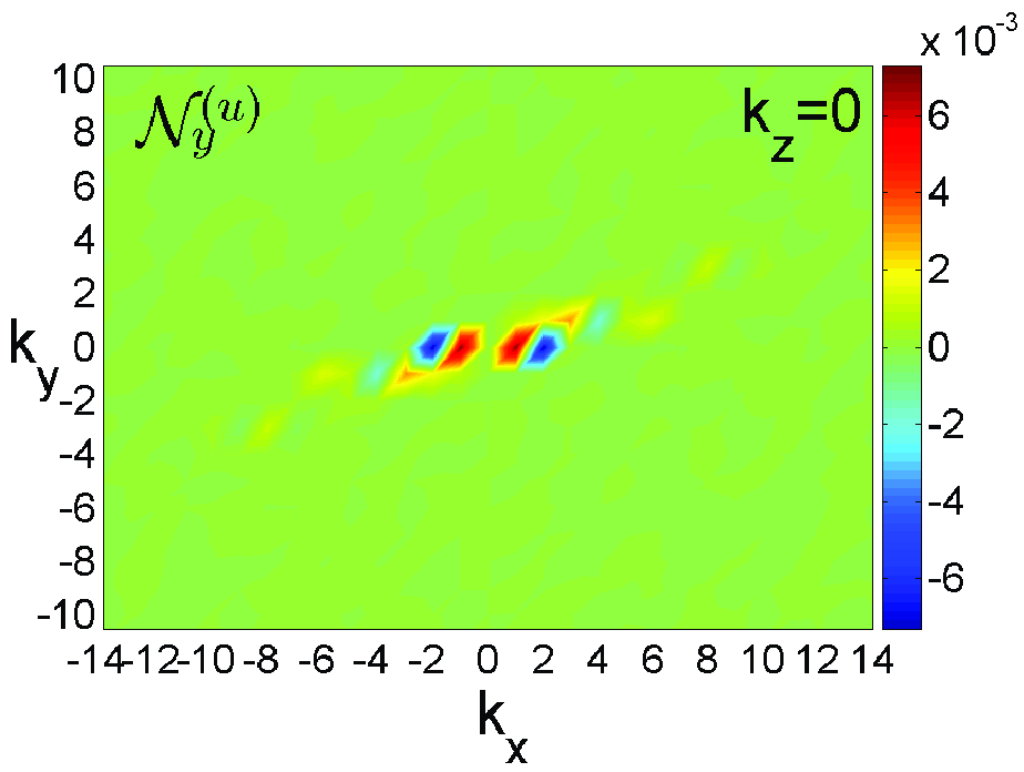
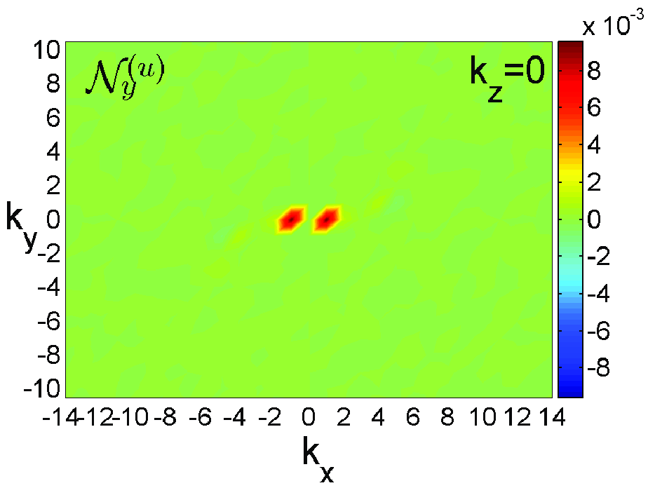
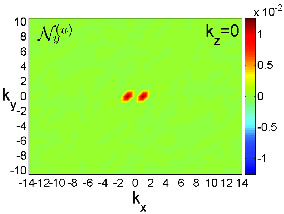
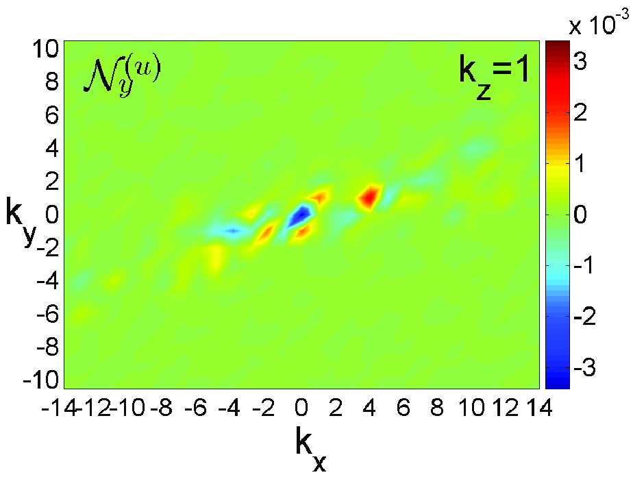
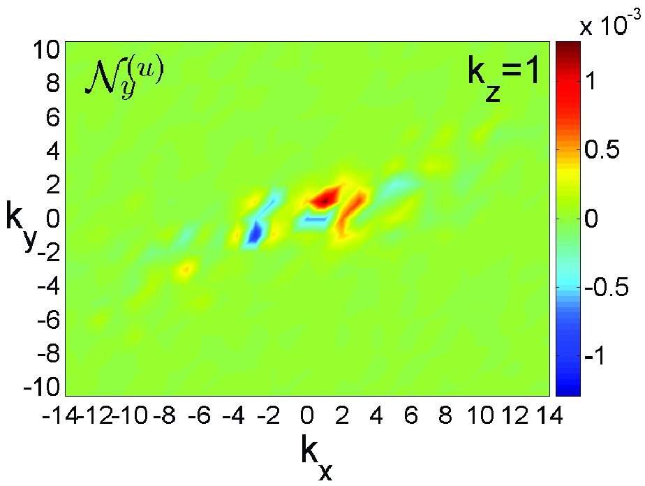
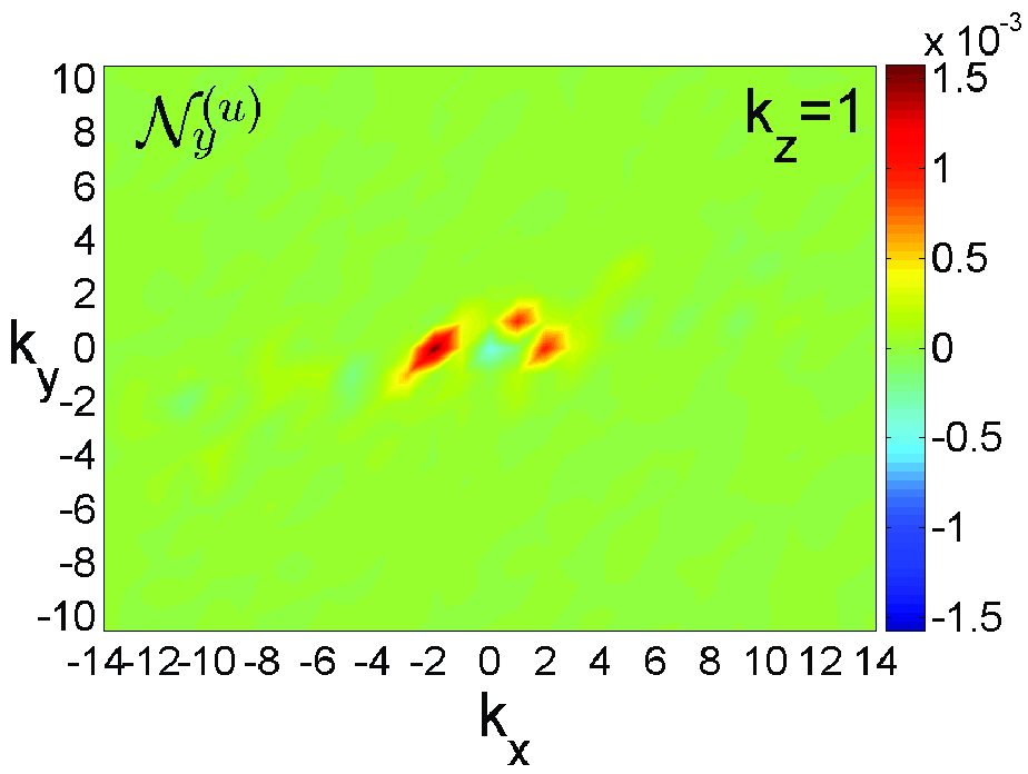
Figure 13: The nonlinear transfer term ${\cal N}_{y}^{(u)}$ in $(k_{x},k_{y})$-plane at $k_{z}=0,1$, when the channel mode energy is at the minimum, i.e., at the end (“bottom”) of the burst at there different moments, $t=296,311,383$. This term is positive at the wavenumber of the zonal flow mode, ${\bf k}_{zf}$, but negative at the wavenumber of the channel mode, ${\bf k}_{c}$, at all these moments. Hence, ${\cal N}_{y}^{(u)}$ at the end of the channel mode burst acts as the source for the zonal flow mode. In other words, the formation of the zonal flow mode starts after the end of the channel mode burst.

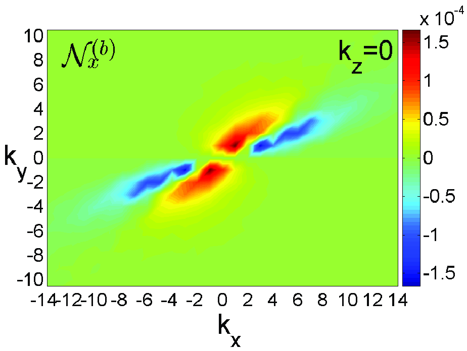
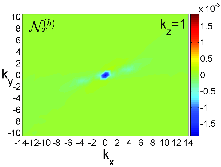
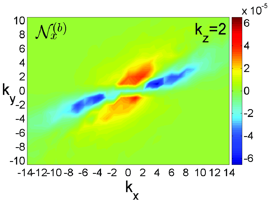
Figure 14: Time-averaged nonlinear term ${\cal N}_{x}^{(b)}$ in $(k_{x},k_{y})$-plane at $k_{z}=0(left),1(middle),2(right)$. As in a single instant shown in Figure 12, the action of this term is highly anisotropic due to the shear, i.e., strongly depend on the wavevector polar angle. However, this time-averaged distribution is much smoother than its instantaneous counterpart and clearly shows transfer of modes over wavevector angles, that is, the transverse cascade of $|\bar{b}_{x}|^{2}$ from the blue regions, where ${\cal N}_{x}^{(b)}<0$ and acts as a sink for it, to the red and yellow regions, where ${\cal N}_{x}^{(b)}>0$ and acts as a source/production. In light green regions, these terms are small, although, as we checked, preserve the same anisotropic shape. As in Figure 12, at $k_{z}=1$, ${\cal N}_{x}^{(b)}$ peaks again at $k_{x}=k_{y}=0$, implying that also in the time-averaged sense, the dominant nonlinear process at $k_{z}=1$ is draining of the channel mode energy and transferring it to the rest modes with other $k_{z}$ (mainly $k_{z}=0,1$).

4.6 Interdependence of the channel, zonal flow and rest modes

So far we have separately described the dynamics of the main – the channel, the zonal flow and the rest modes. Now we move to the analysis of their interlaced dynamics in Fourier space, which determines the properties and balances of MRI-turbulence with net vertical magnetic field. First of all it is a characteristic burst-like behavior of the volume-averaged energies and stresses (Figures 3), which is related to the manifestations of these modes’ activity and nonlinear interaction. As was discussed in subsection 4.3, the short bursts of the channel mode arise as a result of the competition between the linear nonmodal MRI-amplification and nonlinear redistribution of the channel mode’s energy in ${\bf k}$-space. Each such burst event starts with the linear amplification, which initially overwhelms the nonlinear redistribution to other modes and therefore the energy of the channel mode increases. At the same time, the effect of the nonlinear terms on the channel mode, described by ${\cal N}^{(b)}({\bf k}_{c}),{\cal N}^{(u)}({\bf k}_{c})$, increases as well, as it gradually loses its energy to the rest modes due to nonlinear transfers. At a certain amplitude of the channel mode, these nonlinear terms become comparable to the linear ones that are responsible for MRI, halt the further growth of the channel mode and start its fast drain (Figure 8). This moment, corresponding to the peak of the channel mode energy and stress, is a critical stage in its evolution and therefore it is important to examine in more detail how nonlinear processes redistribute/transfer the energy of the channel mode in Fourier space at this time. For this purpose, we present the map of the nonlinear transfer terms in $(k_{x},k_{y})$-plane at $k_{z}=0,1,2$ at two key stages of the burst dynamics – first when the channel mode energy has a peak (Figure 12) and when its energy is at a minimum (Figure 13). The nonlinear redistribution quite differ from each other at these “top” and “bottom” points of the channel mode bursts. In both moments they are notably anisotropic due to the shear, i.e., depend on a wavenumber polar angle, being preferably concentrated in the first and third quadrants, and thus realize the transverse cascade of the modes in Fourier space. Figure 12, corresponding to the “top” in the vicinity of the moment $t=294$ of the highest magnetic energy peak of the channel mode, shows strong negative peaks of the nonlinear transfer terms ${\cal N}_{x}^{(b)}$, ${\cal N}_{y}^{(b)}$, ${\cal N}_{x}^{(u)}$ for the channel mode (i.e., at $k_{x}=k_{y}=0,k_{z}=1$), as the nonlinearity leads its fast drain at this moment. The red and yellow areas in this figure represent the subset of the rest modes, mostly with $k_{z}=0,2$, which receive energy via nonlinear transfers at this moment of the channel mode’s peak activity. Note that at this time, the nonlinearity transfers the channel mode energy not to the zonal flow mode (since ${\cal N}_{y}^{(u)}({\bf k}_{zf})<0$ at this moment), but to the rest modes. In other words, the rest modes can be considered as the main “culprits/parasites” in the decline of the channel mode in the developed turbulent state. The action of the above nonlinear terms in Fourier space during other peaks of the channel mode are qualitatively similar to that given in Figure 12 at around $t=294$, however, concretely which modes, from the total set of the rest modes, receive energy is, of course, different for each burst.

Thus, this unifying approach – the analysis of the dynamics and the nonlinear transfer functions in Fourier space – enables us to self-consistently describe the interaction between the channel and the rest (parasitic) modes when the standard assumptions in the usual treatment of these modes (Goodman & Xu, 1994; Pessah & Goodman, 2009) break down: the amplitudes of these two mode types become comparable, so that one can no longer separate the channel as a primary background and parasites as small perturbations on top of that. Overall, the rest (parasitic) modes play a major role in the channel mode decline. After each its burst, the transverse cascade determines a specific spectrum of the parasitic modes in the turbulent state, which mostly gain energy as a result of draining the channel mode.

Quite differently acts the nonlinearity at the “bottom” point when the channel mode is at its minimum. In this case, the main effect is the production of the zonal flow mode, so that in Figure 13 we show only the nonlinear transfer term for the azimuthal velocity, ${\cal N}_{y}^{(u)}$, at the end (“bottom”) of the channel burst at there different moments. It is seen that this term is positive at the wavenumber of the zonal flow mode, ${\bf k}_{zf}$, at all there moments (red dots at $k_{x}=\pm 1,k_{y}=0$ on the plots with $k_{z}=0$), acting as the source for the zonal flow mode. As a result, the formation of the zonal flow mode starts after the end of the channel mode burst. For the channel mode wavenumber ${\bf k}_{c}$, ${\cal N}_{y}^{(u)}$ is negative at these moments, acting as a sink. As for the other nonlinear terms at the “bottom” points (not shown here), they look qualitatively similar to those in Figure 12, except that they no longer have a prominent negative peak at ${\bf k}_{c}$, since the rest and the zonal flow modes dominate instead in the dynamics at these times.

We have seen from Figures 12 and 13 that the shear-induced anisotropy of nonlinear transfers in Fourier space lie at the basis of the balances of dynamical processes in vertical field MRI-turbulence. In particular, they determine the drain of the channel mode and the resulting anisotropic spectrum of the rest modes which gain energy after each peak of the channel mode. However, the snapshots of the spectral dynamics of the modes shown in these figures, being at separate moments, are still irregular, somewhat obscuring this generic spectral anisotropy of the MRI-turbulence due to the shear. They convey only a short-time behavior of the turbulence. The spectral anisotropy of MRI-turbulence with a net vertical field was demonstrated by Hawley et al. (1995); Lesur & Longaretti (2011) and recently in more detail by Murphy & Pessah (2015), who, however, characterized only the anisotropic spectra of the magnetic energy and Maxwell stress in ${\bf k}$-space, but not the nonlinear processes. This inherent anisotropic character of the dynamical process of shear flows in Fourier space is best identified and described by considering a long-term evolution of the turbulence, i.e., by averaging the spectral quantities over time, as was done in the above studies. Such an averaging in the present case with a net vertical field indeed shows the dominance of the nonlinear transverse cascade, i.e., the angular (i.e., over wavevector angles) redistribution of the power in Fourier space in the overall dynamical balances (nonlinear interactions) between the channel and the rest modes, which is a main process underlying the turbulence. Previously, Lesur & Longaretti (2011) also investigated the nonlinear transfers in a net vertical field MRI-turbulence, however, they applied, together with time-averaging, also shell-averaging of the linear and nonlinear dynamical terms in ${\bf k}$-space that naturally smears out the spectral anisotropy and hence the transverse cascade.

We demonstrate the anisotropic nature of the nonlinear transfers on longer time-scale on the example of the radial component of the magnetic field, for which it is most apparent. Figure 14 shows the corresponding nonlinear term ${\cal N}_{x}^{(b)}$ in $(k_{x},k_{y})$-plane at different $k_{z}=0,1,2$ averaged in time from $t=100$ till $t=650$. Like in a single instant shown in Figure 12, the action of this term is highly anisotropic, that is, depends strongly on the azimuthal angle in $(k_{x},k_{y})$-plane due to the shear. However, this time-averaged distribution is much smoother than its instantaneous counterpart and clearly shows transfer of modes over wavevector angles, i.e., the transverse cascade of $|\bar{b}_{x}|^{2}$ from the blue regions, where ${\cal N}_{x}^{(b)}<0$ and acts as a sink for it, to the red and yellow regions, where ${\cal N}_{x}^{(b)}>0$ and acts as a source/production. In light green regions (outside the vital area) these terms are small, although preserve the same anisotropic shape. As in Figure 12, at $k_{z}=1$, ${\cal N}_{x}^{(b)}$ has a pronounced negative peak again at $k_{x}=k_{y}=0$ in Figure 14, implying that in this time-averaged sense too the dominant nonlinear process at $k_{z}=1$ is draining of the channel mode energy. This energy is transferred transversely to the rest modes with other $k_{z}$ (mainly $k_{z}=0,1$) and a range of $k_{x},k_{y}$ indicated by the red and yellow areas in Figure 14 where ${\cal N}_{x}^{(b)}>0$. Since time-averaging procedure spans the whole duration of the turbulence in the simulations, these smooth regions in fact enclose all the rest modes ever excited during the entire evolution.

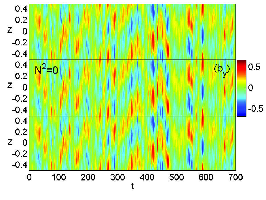
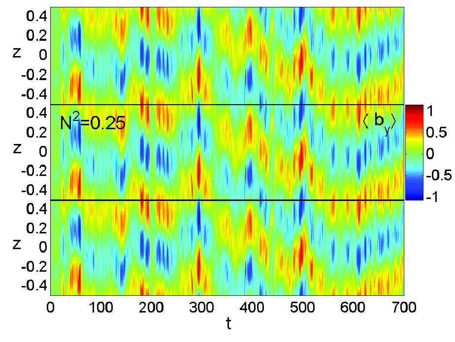
Figure 15: Space-time diagram of the azimuthal field averaged in the horizontal $(x,y)$-plane, $\langle b_{y}\rangle$, in the unstratified $N^{2}=0$ (top) and stratified $N^{2}=0.25$ (bottom) boxes. In contrast to the unstratified case, the stratification results in a remarkable organization of the average azimuthal field, which is dominated by the $k_{z}=\pm 1$ modes, into a relatively coherent pattern in the $(t,z)$-plane with a regular phase variation. Each box has been stacked with identical boxes from top and bottom to ease perception of this pattern.

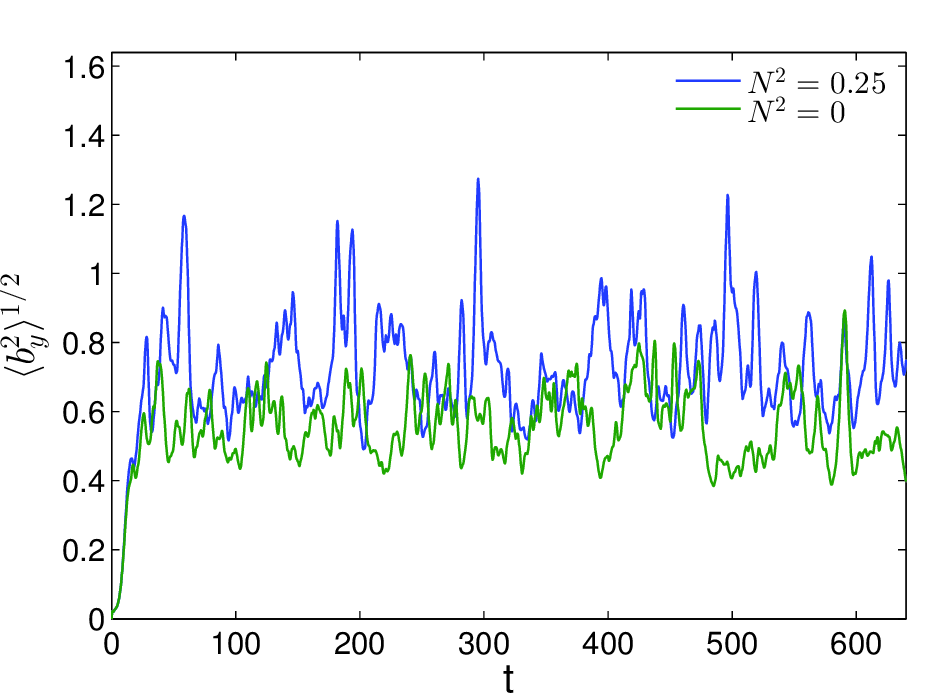
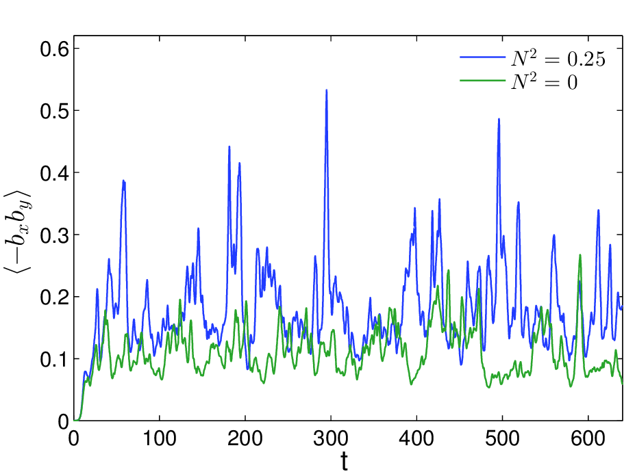
Figure 16: Evolution of the volume-averaged rms of $b_{y}$ (upper panel) and Maxwell stress $\langle-b_{x}b_{y}\rangle$ (lower panel) in the stratified fiducial run at $N^{2}=0.25$ (blue) and unstratified $N^{2}=0$ run (green). In the presence of stratification, both these quantities are larger and exhibit more pronounced burst-like behavior compared to those in the unstratified case.

4.7 On the effect of stratification

It is well-known from simulations of zero net flux MRI-turbulence that vertical stratification favors notable dynamo action in magnetized disks, whereby a large-scale azimuthal magnetic field is generated and exhibits a “butterfly” diagram – regular quasi-periodic spatio-temporal oscillations (reversals) (e.g., Brandenburg et al., 1995; Johansen et al., 2009; Davis et al., 2010; Gressel, 2010; Shi et al., 2010; Simon et al., 2011; Bodo et al., 2012, 2014; Gressel & Pessah, 2015). By contrast, although large-scale azimuthal field generation can still take place in unstratified zero net flux MRI-turbulence in vertically sufficiently extended boxes, the spatio-temporal variation of this field is still more incoherent/irregular in the form of wandering patches (Lesur & Ogilvie, 2008; Shi et al., 2016). A detailed physical mechanism of how stratification brings about such an organization of the magnetic field is not fully understood and requires further studies. This is an important topical question, as it closely bears on the convergence problem in zero net flux MRI-turbulence simulations in stratified and unstratified shearing boxes, which is currently under debate (see e.g., Bodo et al., 2014; Shi et al., 2016; Ryan et al., 2017, and references therein). Despite the fact that the present problem, containing a nonzero net vertical flux, differs from the case of zero net flux usually considered in the context of MRI-dynamo, here we also observe a notable spatio-temporal organization of the large-scale azimuthal field in the turbulent state (see below).

An ordered cyclic behavior of characteristic quantities in MRI-turbulence with a net vertical magnetic flux in the shearing box model, but with more complex isothermal vertical stratification and outflow boundary conditions in the vertical direction, was also found. In particular, Suzuki & Inutsuka (2009) analyzed quasi-periodic variations of the horizontally averaged vertical mass flux (wind) in MRI-turbulent disks and Bai & Stone (2013); Fromang et al. (2013); Simon et al. (2013); Salvesen et al. (2016) showed a similar oscillatory behavior for mean azimuthal magnetic field, which is somewhat analogous to that found in our setup.

The considered here disk flow configuration is based on the Boussinesq approximation, where vertical stratification enters the governing perturbation Equations (A25)-(A27) in a simpler manner than in the above studies – through buoyancy-induced terms, proportional to the vertically uniform Brunt-V$\ddot{\rm a}$is$\ddot{\rm a}$l$\ddot{\rm a}$ frequency squared, $N^{2}$. Still, this simplification has an advantage in that one could simply put only $N^{2}$ to zero in these dynamical equations without altering other parameters and equilibrium configuration of the system. This allows us to directly compare to the unstratified case and more conveniently isolate the basic role of stratification in the dynamo action. In the linear regime, stratification has only a little influence on the dynamics of vertical field MRI (Mamatsashvili et al., 2013). Moreover, it is easily seen that the effect of stratification identically vanishes for the most effectively amplified channel mode with $k_{x}=k_{y}=0$, whose azimuthal field, equal to the averaged in the horizontal $(x,y)$-plane total azimuthal field, in fact constitutes the large-scale dynamo field. So, the effect of stratification on the dynamo action is solely attributable to nonlinearity, which modifies the electromotive force.

Figure 15 shows the space-time diagrams of the horizontally averaged azimuthal magnetic field, $\langle b_{y}\rangle$, in the stratified fiducial case with $N^{2}=0.25$ as used in the paper and unstratified, $N^{2}=0$, case for the same other parameters. It is clearly seen that stratification causes a remarkable organization of the azimuthal field into a coherent wave-like pattern in contrast to the unstratified case. In both cases, however, this horizontally averaged field is dominated by the $k_{z}=\pm 1$ harmonics, i.e., it is associated with the dominant channel mode analyzed above, but its phase variation with $t$ and $z$ in the stratified case is much more regular than that in the unstratified one. The amplitude of this averaged azimuthal field is about an order of magnitude larger than that of the background vertical field $B_{0z}$. Figure 16 shows that the rms of the azimuthal field and the volume-averaged Maxwell stress in the stratified case are larger, with stronger/higher and more frequent bursts, than those in the unstratified case. Clearly, the space-time diagram shown in Figure 15 in the stratified case with periodic vertical boundary conditions differs from a typical “butterfly” observed in the case of isothermal stratification in the above mentioned studies. This difference can be attributable to the different nature of the buoyancy term and vertical boundary conditions used, which jointly cause elevation of the azimuthal flux from the midplane. Nevertheless, this comparison clearly demonstrates the capability of stratification to order/regularize the spatio-temporal variation of the mean azimuthal field – the main field component in accretion disk dynamo. Here, we have presented only a primary manifestation of the effect of stratification in the net vertical field MRI-turbulence. In its own right, it is a subject of a detailed and refined investigation.

5 Summary and discussions

In this paper, we investigated the dynamical balances underlying MRI-driven turbulence in Keplerian disks with a nonzero net vertical magnetic field and vertically uniform thermal stratification using shearing box simulations. Focusing on the analysis of the turbulence dynamics in Fourier (${\bf k}$-) space, we identified three key types of modes – the channel, the zonal flow mode and the rest modes – that are the main “players” in the turbulence dynamics. We described the dynamics of these modes separately and then their interdependence, which sets the properties of the nonzero net vertical field MRI-turbulence. The processes of linear origin are defined primarily by nonmodal, rather than modal, growth of MRI due to disk flow nonnormality/shear. This is because the dynamical time of the turbulence is of the order of the orbital/shear time during which the nonmodal effects are important. In the turbulent state, higher values of the stresses and magnetic energy fall just on those active modes that exhibit high nonmodal MRI growth and not on the modally (exponentially) most unstable modes. In other words, the properties of the turbulence are determined mostly by nonmodal physics of MRI rather than by the modal one. From all the active modes, the one that exhibits the maximum nonmodal growth is the channel mode, which is horizontally uniform with the largest vertical scale in the domain. As for the nonlinear processes, it can be confidently stated that the decisive agent in forming and maintaining the statistical characteristics of the net vertical field MRI-turbulence is the transverse cascade – nonlinear redistribution of modes in Fourier space that changes the orientation (angle) of their wavevectors – arising from the presence of the shear and hence being a generic phenomenon in shear flows. Specifically, the nonlinear transverse cascade redistributes the energy of the channel mode to the rest modes and, subsequently, the energy of the rest modes to the zonal flow mode. (One has to note that the rest modes receive energy not only due to the nonlinear transfers, but they themselves also undergo nonmodal transient growth, however, less than the channel mode does). The combined action of these linear and nonlinear processes leads to the channel mode exhibiting recurrent bursts of the energy and stresses. The nonlinear transfer of its energy to the rest modes causes the decline of the channel mode after each burst and subsequent abrupt increase of the energy of the rest modes. This, in turn, induces similar, burst-like evolution of the integral characteristics of the turbulence – the total volume-averaged energies, stresses and transport.

The rest modes here, playing the main role in draining the channel mode, were referred to as parasitic modes in previous studies of net vertical field MRI. However, there is an important distinction. These parasitic modes are often assumed to be small compared with the channel mode and are treated as linear perturbations imposed on the latter (Goodman & Xu, 1994; Pessah & Goodman, 2009; Latter et al., 2009, 2010; Pessah, 2010). Besides, the effect of shear and hence the nonmodal (transient) physics are neglected with respect to parasitic modes. In the turbulent state, however, the rest modes can reach energies comparable to the channel mode, as has been demonstrated in this paper, so one can no longer separate the channel as a primary background and parasites as small perturbations on top of that. As a result, the complex interaction between these two mode types belongs to the domain of nonlinearity. Our general/unifying approach – the analysis of the dynamics in 3D Fourier space – allows us to self-consistently characterize this interaction of the modes. In this case, the transverse cascade defines the spectrum of the rest modes, which contribute to the decline of the channel mode after each burst and subsequently acquire energy in this process.

As we found in this study, the net vertical field MRI-turbulence is robust and, in addition, multifarious – determined by the interdependent/interlaced dynamics of three qualitatively different modes. Consequently, in order to properly quantify the relative contribution of each of these modes in the turbulence characteristics, one has to capture the main aspects of their dynamics in numerical simulations. First of all, this concerns the selection of relevant sizes (aspect ratio) of the simulation box (which is actually arbitrary in the shearing box framework) and resolutions, so that the discrete modes in the selected box densely enough cover the vital area in $(k_{x},k_{y})$-plane and maximally comprise effectively growing (optimal) modes (see Figure 1). Besides, one should also avoid artificial/numerical anisotropyzation of nonlinear processes. As was shown in Paper I, the anisotropy of the simulation box in $(k_{x},k_{y})$-plane introduces artificial anisotropy of nonlinear processes and somewhat “deforms” the overall dynamical picture of MRI-turbulence in Fourier space. In the present case, this artificial deformation could result in a change of the relative importance of the above-classified modes in the overall dynamics, for instance, could reduce the effectiveness of the channel mode compared to other modes and hence weaken its manifestation in the turbulence dynamics (see e.g., Bodo et al., 2008). In particular, changing the role of the large-scale channel mode likely affects the generation of the mean azimuthal magnetic field, or the dynamo action, since this field is directly associated with this mode. Susceptibility of the latter to specific factors of the dynamics is clearly shown in Figure 15: although the vertical stratification makes only negligible contribution to the turbulence energy, it remarkably enhances the generation of the mean azimuthal magnetic field and regularizes its spatio-temporal variation. The latter process is significant and represents the subject of a special detailed investigation.

5.1 On types of anisotropy

Apart from the analyzed in our paper shear-induced anisotropy of the nonlinear processes, a net nonzero background magnetic field itself, by definition, gives rise to anisotropy of the nonlinear dynamics to its parallel and perpendicular directions. However, these two types of anisotropy, having different origin, essentially differ from each other.

Anisotropy of nonlinear cascade processes due to magnetic field (directed along $z$-axis) in plasmas with static equilibrium is analyzed in Goldreich & Sridhar (1995). The source of energy is assumed to be isotropic in both physical and Fourier spaces with some outer scale of turbulence, $L$, corresponding to the smallest wavenumber, $k_{0}\sim 1/L$. Nonlinear cascade processes take place in the inertial range, at perpendicular and parallel to the field wavenumbers $k_{\perp},k_{z}\gtrsim k_{0}$, which is in fact the region of activity of these processes only. Overall, the regions of the energy supply and nonlinear cascade in Fourier space are separated from each other. As a result, the nonlinear processes do not affect the turbulence energy supply – they only transfer energy mainly to small perpendicular (to the magnetic field) wavelength, i.e., to large $k_{\perp}$ rather than along $k_{z}$, thereby forming anisotropic spectrum of the turbulence in $(k_{\perp},k_{z})$-plane. This nonlinear cascade mostly to large $k_{\perp}$, besides increasing the magnitude $k=\sqrt{k_{\perp}^{2}+k_{z}^{2}}$ of the total wavevector, ${\bf k}=(k_{\perp},k_{z})$ (direct cascade), by definition, implies also a change of its orientation that results in some angular redistribution of harmonics (i.e., transverse cascade). At $k_{\perp}/k_{z}\sim 1$, the direct and transverse cascades are comparable. As the cascade proceeds, the ratio $k_{\perp}/k_{z}$ increases, leading ${\bf k}$ to change primarily in magnitude rather than in orientation and hence the direct cascade becomes dominant. In any case, the angular redistribution (transverse cascade) in this case is of secondary importance – does not affect the turbulence energy supply.

A completely different situation arises in the presence of the disk flow shear. Linear (nonmodal) energy supply processes of perturbations/turbulence in shear flows are strongly anisotropic in Fourier space and generally occur over a broad range of wave numbers without leaving a free room (i.e., inertial range) for the action of nonlinear processes only. Due to the inherent anisotropy of the linear dynamics due to the shear, the nonlinear processes in this range of wavenumbers become strongly anisotropic, i.e., the transverse cascade is the dominant nonlinear process. Overall, dynamical picture of the turbulence is formed as a result of the interplay of the linear and nonlinear (transverse cascade) processes. The area of the most intensive interplay of the linear and nonlinear processes we call the vital area of the turbulence. Of course, the nonlinear processes leads to energy exchange between different modes, redistributing perturbation energy in Fourier space while leaving the total energy unchanged. However, the nonlinear transverse cascade in shear flows repopulates the (transiently) growing harmonics and, in this way, indirectly contributes to the energy supply to turbulence. As we have shown above, in the present problem of net vertical field MRI-turbulence in Keplerian shear flow, it significantly affects the dynamical “design” of the turbulence and determines the interplay of its “building blocks” – channel, zonal flow and the rest modes. This is clearly illustrated by Figures 12-14, showing resulting anisotropic dynamics (transfers) in $(k_{x},k_{y})$-plane perpendicular to the field. By contrast, in the absence of basic flow velocity shear, nonlinear cascades in this plane are isotropic in Goldreich & Sridhar theory.

Appendix A Perturbation equations in physical and Fourier space

From the main Equations (1)-(5) one can derive equations for the perturbations, ${\bf u},p,{\bf b}$, of arbitrary amplitude about the Keplerian shear flow ${\bf U}_{0}=-q\Omega x{\bf e}_{y}$ with a net vertical field ${\bf B}_{0}=B_{0z}{\bf e}_{z}$:

$$\frac{Du_{x}}{Dt}=2\Omega u_{y}-\frac{1}{\rho_{0}}\frac{\partial p}{\partial x}+\frac{B_{0z}}{4\pi\rho_{0}}\frac{\partial b_{x}}{\partial z}+\frac{\partial}{\partial x}\left(\frac{b_{x}^{2}}{4\pi\rho_{0}}-u_{x}^{2}\right)+\frac{\partial}{\partial y}\left(\frac{b_{x}b_{y}}{4\pi\rho_{0}}-u_{x}u_{y}\right)+\frac{\partial}{\partial z}\left(\frac{b_{x}b_{z}}{4\pi\rho_{0}}-u_{x}u_{z}\right)+\nu\nabla^{2}u_{x},$$ (A1)

$$\frac{Du_{y}}{Dt}=(q-2)\Omega u_{x}-\frac{1}{\rho_{0}}\frac{\partial p}{\partial y}+\frac{B_{0z}}{4\pi\rho_{0}}\frac{\partial b_{y}}{\partial z}+\frac{\partial}{\partial x}\left(\frac{b_{x}b_{y}}{4\pi\rho_{0}}-u_{x}u_{y}\right)+\frac{\partial}{\partial y}\left(\frac{b_{y}^{2}}{4\pi\rho_{0}}-u_{y}^{2}\right)+\frac{\partial}{\partial z}\left(\frac{b_{z}b_{y}}{4\pi\rho_{0}}-u_{z}u_{y}\right)+\nu\nabla^{2}u_{y}$$ (A2)

$$\frac{Du_{z}}{Dt}=-\frac{1}{\rho_{0}}\frac{\partial p}{\partial z}-\theta+\frac{B_{0z}}{4\pi\rho_{0}}\frac{\partial b_{z}}{\partial z}+\frac{\partial}{\partial x}\left(\frac{b_{x}b_{z}}{4\pi\rho_{0}}-u_{x}u_{z}\right)+\frac{\partial}{\partial y}\left(\frac{b_{y}b_{z}}{4\pi\rho_{0}}-u_{y}u_{z}\right)+\frac{\partial}{\partial z}\left(\frac{b_{z}^{2}}{4\pi\rho_{0}}-u_{z}^{2}\right)+\nu\nabla^{2}u_{z}$$ (A3)

$$\frac{D\theta}{Dt}=N^{2}u_{z}-\frac{\partial}{\partial x}(u_{x}\theta)-\frac{\partial}{\partial y}(u_{y}\theta)-\frac{\partial}{\partial z}(u_{z}\theta)+\chi\nabla^{2}\theta$$ (A4)

$$\frac{Db_{x}}{Dt}=B_{0z}\frac{\partial u_{x}}{\partial z}+\frac{\partial}{\partial y}\left(u_{x}b_{y}-u_{y}b_{x}\right)-\frac{\partial}{\partial z}(u_{z}b_{x}-u_{x}b_{z})+\eta\nabla^{2}b_{x},$$ (A5)

$$\frac{Db_{y}}{Dt}=-q\Omega b_{x}+B_{0z}\frac{\partial u_{y}}{\partial z}-\frac{\partial}{\partial x}\left(u_{x}b_{y}-u_{y}b_{x}\right)+\frac{\partial}{\partial z}(u_{y}b_{z}-u_{z}b_{y})+\eta\nabla^{2}b_{y},$$ (A6)

$$\frac{Db_{z}}{Dt}=B_{0z}\frac{\partial u_{z}}{\partial z}+\frac{\partial}{\partial x}\left(u_{z}b_{x}-u_{x}b_{z}\right)-\frac{\partial}{\partial y}(u_{y}b_{z}-u_{z}b_{y})+\eta\nabla^{2}b_{z},$$ (A7)

$$\frac{\partial u_{x}}{\partial x}+\frac{\partial u_{y}}{\partial y}+\frac{\partial u_{z}}{\partial z}=0,$$ (A8)

$$\frac{\partial b_{x}}{\partial x}+\frac{\partial b_{y}}{\partial y}+\frac{\partial b_{z}}{\partial z}=0,$$ (A9)

where $D/Dt=\partial/\partial t-q\Omega x\partial/\partial y$ is the total derivative along the background flow.

Substituting decomposition (6) into Equations (A1)-(A9) and taking into account the normalization, we obtain the evolution equations for the Fourier modes:

$$\left(\frac{\partial}{\partial t}+qk_{y}\frac{\partial}{\partial k_{x}}\right)\bar{u}_{x}=2\bar{u}_{y}-{\rm i}k_{x}\bar{p}+{\rm i}k_{z}B_{0z}\bar{b}_{x}-\frac{k^{2}}{\rm Re}\bar{u}_{x}+{\rm i}k_{x}N^{(u)}_{xx}+{\rm i}k_{y}N^{(u)}_{xy}+{\rm i}k_{z}N^{(u)}_{xz},$$ (A10)

$$\left(\frac{\partial}{\partial t}+qk_{y}\frac{\partial}{\partial k_{x}}\right)\bar{u}_{y}=(q-2)\bar{u}_{x}-{\rm i}k_{y}\bar{p}+{\rm i}k_{z}B_{0z}\bar{b}_{y}-\frac{k^{2}}{\rm Re}\bar{u}_{y}+{\rm i}k_{x}N^{(u)}_{xy}+{\rm i}k_{y}N^{(u)}_{yy}+{\rm i}k_{z}N^{(u)}_{yz},$$ (A11)

$$\left(\frac{\partial}{\partial t}+qk_{y}\frac{\partial}{\partial k_{x}}\right)\bar{u}_{z}=-{\rm i}k_{z}\bar{p}-\bar{\theta}+{\rm i}k_{z}B_{0z}\bar{b}_{z}-\frac{k^{2}}{\rm Re}\bar{u}_{z}+{\rm i}k_{x}N^{(u)}_{xz}+{\rm i}k_{y}N^{(u)}_{yz}+{\rm i}k_{z}N^{(u)}_{zz},$$ (A12)

$$\left(\frac{\partial}{\partial t}+qk_{y}\frac{\partial}{\partial k_{x}}\right)\bar{\theta}=N^{2}\bar{u}_{z}-\frac{k^{2}}{\rm Pe}\bar{\theta}+{\rm i}k_{x}N^{(\theta)}_{x}+{\rm i}k_{y}N^{(\theta)}_{y}+{\rm i}k_{z}N^{(\theta)}_{z},$$ (A13)

$$\left(\frac{\partial}{\partial t}+qk_{y}\frac{\partial}{\partial k_{x}}\right)\bar{b}_{x}={\rm i}k_{z}B_{0z}\bar{u}_{x}-\frac{k^{2}}{\rm Rm}\bar{b}_{x}+{\rm i}k_{y}\bar{F}_{z}-{\rm i}k_{z}\bar{F}_{y},$$ (A14)

$$\left(\frac{\partial}{\partial t}+qk_{y}\frac{\partial}{\partial k_{x}}\right)\bar{b}_{y}=-q\bar{b}_{x}+{\rm i}k_{z}B_{0z}\bar{u}_{y}-\frac{k^{2}}{\rm Rm}\bar{b}_{y}+{\rm i}k_{z}\bar{F}_{x}-{\rm i}k_{x}\bar{F}_{z}$$ (A15)

$$\left(\frac{\partial}{\partial t}+qk_{y}\frac{\partial}{\partial k_{x}}\right)\bar{b}_{z}={\rm i}k_{z}B_{0z}\bar{u}_{z}-\frac{k^{2}}{\rm Rm}\bar{b}_{z}+{\rm i}k_{x}\bar{F}_{y}-{\rm i}k_{y}\bar{F}_{x}$$ (A16)

$$k_{x}\bar{u}_{x}+k_{y}\bar{u}_{y}+k_{z}\bar{u}_{z}=0,$$ (A17)

$$k_{x}\bar{b}_{x}+k_{y}\bar{b}_{y}+k_{z}\bar{b}_{z}=0,$$ (A18)

where $k^{2}=k_{x}^{2}+k_{y}^{2}+k_{z}^{2}$ and $B_{0z}=\sqrt{2/\beta}$ is the normalized constant background field. These spectral equations involve the linear and nonlinear ($N^{(u)}_{ij}({\bf k},t),N^{(\theta)}_{i}({\bf k},t),\bar{F}_{i}({\bf k},t)$, where $i,j=x,y,z$) terms that are the Fourier transforms of the corresponding linear and nonlinear terms of Equations (A1)-(A9) in physical space. These nonlinear terms are given by convolutions

$$N^{(u)}_{ij}({\bf k},t)=\int d^{3}{\bf k^{\prime}}\left[\bar{b}_{i}({\bf k^{\prime}},t)\bar{b}_{j}({\bf k}-{\bf k^{\prime}},t)-\bar{u}_{i}({\bf k^{\prime}},t)\bar{u}_{j}({\bf k}-{\bf k^{\prime}},t)\right],$$ (A19)

$$N^{(\theta)}_{i}({\bf k},t)=-\int d^{3}{\bf k^{\prime}}\bar{u}_{i}({\bf k^{\prime}},t)\bar{\theta}({\bf k}-{\bf k^{\prime}},t)$$ (A20)

and $\bar{F}_{x},\bar{F}_{y},\bar{F}_{z}$, which are the Fourier transforms of the respective components of the perturbed electromotive force ${\bf F}={\bf u}\times{\bf b}$,

$$\bar{F}_{x}({\bf k},t)=\int d^{3}{\bf k^{\prime}}\left[\bar{u}_{y}({\bf k^{\prime}},t)\bar{b}_{z}({\bf k}-{\bf k^{\prime}},t)-\bar{u}_{z}({\bf k^{\prime}},t)\bar{b}_{y}({\bf k}-{\bf k^{\prime}},t)\right]$$ (A21)

$$\bar{F}_{y}({\bf k},t)=\int d^{3}{\bf k^{\prime}}\left[\bar{u}_{z}({\bf k^{\prime}},t)\bar{b}_{x}({\bf k}-{\bf k^{\prime}},t)-\bar{u}_{x}({\bf k^{\prime}},t)\bar{b}_{z}({\bf k}-{\bf k^{\prime}},t)\right]$$ (A22)

$$\bar{F}_{z}({\bf k},t)=\int d^{3}{\bf k^{\prime}}\left[\bar{u}_{x}({\bf k^{\prime}},t)\bar{b}_{y}({\bf k}-{\bf k^{\prime}},t)-\bar{u}_{y}({\bf k^{\prime}},t)\bar{b}_{x}({\bf k}-{\bf k^{\prime}},t)\right]$$ (A23)

describe the effect of nonlinearity on the magnetic field perturbations. From Equations (A10)-(A12) and the divergence-free conditions (A17) and (A18) we can express pressure

$$\bar{p}=2{\rm i}(1-q)\frac{k_{y}}{k^{2}}\bar{u}_{x}-2{\rm i}\frac{k_{x}}{k^{2}}\bar{u}_{y}+{\rm i}\frac{k_{z}}{k^{2}}\bar{\theta}+\sum_{(i,j)=(x,y,z)}\frac{k_{i}k_{j}}{k^{2}}N^{(u)}_{ij}$$ (A24)

Inserting it back into Equations (A10)-(A12) we have

$$\left(\frac{\partial}{\partial t}+qk_{y}\frac{\partial}{\partial k_{x}}\right)\bar{u}_{x}=2\left(1-\frac{k_{x}^{2}}{k^{2}}\right)\bar{u}_{y}+2(1-q)\frac{k_{x}k_{y}}{k^{2}}\bar{u}_{x}+\frac{k_{x}k_{z}}{k^{2}}\bar{\theta}+{\rm i}k_{z}B_{0z}\bar{b}_{x}-\frac{k^{2}}{\rm Re}\bar{u}_{x}+Q_{x},$$ (A25)

$$\left(\frac{\partial}{\partial t}+qk_{y}\frac{\partial}{\partial k_{x}}\right)\bar{u}_{y}=\left[q-2-2(q-1)\frac{k_{y}^{2}}{k^{2}}\right]\bar{u}_{x}-2\frac{k_{x}k_{y}}{k^{2}}\bar{u}_{y}+\frac{k_{y}k_{z}}{k^{2}}\bar{\theta}+{\rm i}k_{z}B_{0z}\bar{b}_{y}-\frac{k^{2}}{\rm Re}\bar{u}_{y}+Q_{y},$$ (A26)

$$\left(\frac{\partial}{\partial t}+qk_{y}\frac{\partial}{\partial k_{x}}\right)\bar{u}_{z}=2(1-q)\frac{k_{y}k_{z}}{k^{2}}\bar{u}_{x}-2\frac{k_{x}k_{z}}{k^{2}}\bar{u}_{y}-\left(1-\frac{k_{z}^{2}}{k^{2}}\right)\bar{\theta}+{\rm i}k_{z}B_{0z}\bar{b}_{z}-\frac{k^{2}}{\rm Re}\bar{u}_{z}+Q_{z},$$ (A27)

where

$$Q_{i}={\rm i}\sum_{j}k_{j}N^{(u)}_{ij}-{\rm i}k_{i}\sum_{m,n}\frac{k_{m}k_{n}}{k^{2}}N^{(u)}_{mn},~{}~{}~{}~{}~{}i,j,m,n=x,y,z.$$ (A28)

References

- Afshordi et al. (2005) Afshordi, N., Mukhopadhyay, B., & Narayan, R. 2005, ApJ, 629, 373
- Alexakis et al. (2007) Alexakis, A., Mininni, P. D., & Pouquet, A. 2007, New J. Phys., 9, 298
- Bai & Stone (2013) Bai, X.-N., & Stone, J. M. 2013, ApJ, 767, 30
- Bai & Stone (2014) —. 2014, ApJ, 796, 31
- Balbus & Hawley (1991) Balbus, S. A., & Hawley, J. F. 1991, ApJ, 376, 214
- Balbus & Hawley (1992) —. 1992, ApJ, 400, 610
- Balbus & Hawley (1998) —. 1998, Rev. Mod. Phys., 70, 1
- Bodo et al. (2012) Bodo, G., Cattaneo, F., Mignone, A., & Rossi, P. 2012, ApJ, 761, 116
- Bodo et al. (2014) —. 2014, ApJ, 787, L13
- Bodo et al. (2008) Bodo, G., Mignone, A., Cattaneo, F., Rossi, P., & Ferrari, A. 2008, A&A, 487, 1
- Brandenburg & Dintrans (2006) Brandenburg, A., & Dintrans, B. 2006, A&A, 450, 437
- Brandenburg et al. (1995) Brandenburg, A., Nordlund, A., Stein, R. F., & Torkelsson, U. 1995, ApJ, 446, 741
- Chagelishvili et al. (2003) Chagelishvili, G. D., Zahn, J.-P., Tevzadze, A. G., & Lominadze, J. G. 2003, A&A, 402, 401
- Chandrasekhar (1960) Chandrasekhar, S. 1960, Proceedings of the National Academy of Science, 46, 253
- Davis et al. (2010) Davis, S. W., Stone, J. M., & Pessah, M. E. 2010, ApJ, 713, 52
- Farrell & Ioannou (1996) Farrell, B. F., & Ioannou, P. J. 1996, Journal of Atmospheric Sciences, 53, 2025
- Flock et al. (2012) Flock, M., Henning, T., & Klahr, H. 2012, ApJ, 761, 95
- Fromang et al. (2013) Fromang, S., Latter, H., Lesur, G., & Ogilvie, G. I. 2013, A&A, 552, A71
- Fromang & Nelson (2006) Fromang, S., & Nelson, R. P. 2006, A&A, 457, 343
- Fromang & Papaloizou (2007) Fromang, S., & Papaloizou, J. 2007, A&A, 476, 1113
- Gogichaishvili et al. (2017) Gogichaishvili, D., Mamatsashvili, G., Horton, W., Chagelishvili, G., & Bodo, G. 2017, ApJ, 845, 70 (Paper I)
- Goldreich & Sridhar (1995) Goldreich, P., & Sridhar, S. 1995, ApJ, 438, 763
- Goodman & Xu (1994) Goodman, J., & Xu, G. 1994, ApJ, 432, 213
- Gressel (2010) Gressel, O. 2010, MNRAS, 405, 41
- Gressel & Pessah (2015) Gressel, O., & Pessah, M. E. 2015, ApJ, 810, 59
- Guan & Gammie (2011) Guan, X., & Gammie, C. F. 2011, ApJ, 728, 130
- Guan et al. (2009) Guan, X., Gammie, C. F., Simon, J. B., & Johnson, B. M. 2009, ApJ, 694, 1010
- Hawley et al. (1995) Hawley, J., Gammie, C., & Balbus, S. 1995, ApJ, 440, 742
- Hawley & Balbus (1991) Hawley, J. F., & Balbus, S. A. 1991, ApJ, 376, 223
- Hawley & Balbus (1992) —. 1992, ApJ, 400, 595
- Herault et al. (2011) Herault, J., Rincon, F., Cossu, C., et al. 2011, Phys. Rev. E, 84, 036321
- Horton et al. (2010) Horton, W., Kim, J.-H., Chagelishvili, G. D., Bowman, J. C., & Lominadze, J. G. 2010, Phys. Rev. E, 81, 066304
- Johansen et al. (2009) Johansen, A., Youdin, A., & Klahr, H. 2009, ApJ, 697, 1269
- Latter et al. (2015) Latter, H. N., Fromang, S., & Faure, J. 2015, MNRAS, 453, 3257
- Latter et al. (2010) Latter, H. N., Fromang, S., & Gressel, O. 2010, MNRAS, 406, 848
- Latter et al. (2009) Latter, H. N., Lesaffre, P., & Balbus, S. A. 2009, MNRAS, 394, 715
- Lesur & Longaretti (2007) Lesur, G., & Longaretti, P.-Y. 2007, MNRAS, 378, 1471
- Lesur & Longaretti (2011) —. 2011, A&A, 528, A17
- Lesur & Ogilvie (2008) Lesur, G., & Ogilvie, G. I. 2008, A&A, 488, 451
- Lesur & Ogilvie (2010) —. 2010, MNRAS, 404, L64
- Lominadze et al. (1988) Lominadze, D. G., Chagelishvili, G. D., & Chanishvili, R. G. 1988, Sov. Astron. Lett., 14, 364
- Longaretti & Lesur (2010) Longaretti, P.-Y., & Lesur, G. 2010, A&A, 516, A51
- Lynden-Bell & Pringle (1974) Lynden-Bell, D., & Pringle, J. E. 1974, MNRAS, 168, 603
- Mamatsashvili et al. (2016) Mamatsashvili, G., Khujadze, G., Chagelishvili, G., et al. 2016, Phys. Rev. E, 94, 023111
- Mamatsashvili et al. (2013) Mamatsashvili, G. R., Chagelishvili, G. D., Bodo, G., & Rossi, P. 2013, MNRAS, 435, 2552
- Mamatsashvili et al. (2014) Mamatsashvili, G. R., Gogichaishvili, D. Z., Chagelishvili, G. D., & Horton, W. 2014, Phys. Rev. E, 89, 043101
- Meheut et al. (2015) Meheut, H., Fromang, S., Lesur, G., Joos, M., & Longaretti, P.-Y. 2015, A&A, 579, A117
- Murphy & Pessah (2015) Murphy, G. C., & Pessah, M. E. 2015, ApJ, 802, 139
- Nauman & Blackman (2014) Nauman, F., & Blackman, E. G. 2014, MNRAS, 441, 1855
- Papaloizou & Terquem (1997) Papaloizou, J. C. B., & Terquem, C. 1997, MNRAS, 287, 771
- Pessah (2010) Pessah, M. E. 2010, ApJ, 716, 1012
- Pessah & Chan (2008) Pessah, M. E., & Chan, C.-K. 2008, ApJ, 684, 498
- Pessah & Chan (2012) —. 2012, ApJ, 751, 48
- Pessah et al. (2006) Pessah, M. E., Chan, C.-K., & Psaltis, D. 2006, MNRAS, 372, 183
- Pessah & Goodman (2009) Pessah, M. E., & Goodman, J. 2009, ApJ, 698, L72
- Razdoburdin & Zhuravlev (2017) Razdoburdin, D. N., & Zhuravlev, V. V. 2017, MNRAS, 467, 849
- Riols et al. (2017) Riols, A., Rincon, F., Cossu, C., et al. 2017, A&A, 598, A87
- Ryan et al. (2017) Ryan, B. R., Gammie, C. F., Fromang, S., & Kestener, P. 2017, ApJ, 840, 6
- Salhi et al. (2012) Salhi, A., Lehner, T., Godeferd, F., & Cambon, C. 2012, Phys. Rev. E, 85, 026301
- Salvesen et al. (2016) Salvesen, G., Simon, J. B., Armitage, P. J., & Begelman, M. C. 2016, MNRAS, 457, 857
- Sano & Inutsuka (2001) Sano, T., & Inutsuka, S.-I. 2001, ApJ, 561, L179
- Schmid & Henningson (2001) Schmid, P. J., & Henningson, D. S. 2001, Stability and Transition in Shear Flows (Springer)
- Shakura & Postnov (2015) Shakura, N., & Postnov, K. 2015, MNRAS, 448, 3697
- Shakura & Sunyaev (1973) Shakura, N. I., & Sunyaev, R. A. 1973, A&A, 24, 337
- Shi et al. (2010) Shi, J.-M., Krolik, J. H., & Hirose, S. 2010, ApJ, 708, 1716
- Shi et al. (2016) Shi, J.-M., Stone, J. M., & Huang, C. X. 2016, MNRAS, 456, 2273
- Shtemler et al. (2011) Shtemler, Y. M., Mond, M., & Liverts, E. 2011, MNRAS, 413, 2957
- Simon & Armitage (2014) Simon, J. B., & Armitage, P. J. 2014, ApJ, 784, 15
- Simon et al. (2013) Simon, J. B., Bai, X.-N., Armitage, P. J., Stone, J. M., & Beckwith, K. 2013, ApJ, 775, 73
- Simon et al. (2012) Simon, J. B., Beckwith, K., & Armitage, P. J. 2012, MNRAS, 422, 2685
- Simon & Hawley (2009) Simon, J. B., & Hawley, J. F. 2009, ApJ, 707, 833
- Simon et al. (2009) Simon, J. B., Hawley, J. F., & Beckwith, K. 2009, ApJ, 690, 974
- Simon et al. (2011) —. 2011, ApJ, 730, 94
- Squire & Bhattacharjee (2014) Squire, J., & Bhattacharjee, A. 2014, ApJ, 797, 67
- Suzuki & Inutsuka (2009) Suzuki, T. K., & Inutsuka, S.-I. 2009, ApJ, 691, L49
- Tevzadze et al. (2008) Tevzadze, A. G., Chagelishvili, G. D., & Zahn, J.-P. 2008, A&A, 478, 9
- Velikhov (1959) Velikhov, E. 1959, Zh. Eksp. Teor. Fiz., 36, 1398
- Verma (2004) Verma, M. K. 2004, Phys. Rep., 401, 229
- Walker et al. (2016) Walker, J., Lesur, G., & Boldyrev, S. 2016, MNRAS, 457, L39
- Wardle (1999) Wardle, M. 1999, MNRAS, 307, 849
- Yecko (2004) Yecko, P. A. 2004, A&A, 425, 385
- Zhuravlev & Razdoburdin (2014) Zhuravlev, V. V., & Razdoburdin, D. N. 2014, MNRAS, 442, 870