The eruption of a prominence carrying coronal flux rope: forward synthesis of the magnetic field strength measurement by the COronal Solar Magnetism Observatory Large Coronagraph

Abstract

From a magnetohydrodynamic (MHD) simulation of the eruption of a prominence hosting coronal flux rope, we carry out forward synthesis of the circular polarization signal (Stokes V signal) of the FeXIII emission line at 1074.7 nm produced by the MHD model as measured by the proposed COronal Solar Magnetism Observatory (COSMO) Large Coronagraph (LC) and infer the line-of-sight magnetic field $B_{\rm LOS}$ above the limb. With an aperture of 150 cm, integration time of 12 min, and a resolution of 12 arcsec, the LC can measure a significant $B_{\rm LOS}$ with sufficient signal to noise level, from the simulated flux rope viewed nearly along its axis with a peak axial field strength of about 10 G. The measured $B_{\rm LOS}$ is found to relate well with the axial field strength of the flux rope for the height range of the prominence, and can discern the increase with height of the magnetic field strength in that height range that is a definitive signature of the concave upturning dipped field supporting the prominence. The measurement can also detect an outward moving $B_{\rm LOS}$ due to the slow rise of the flux rope as it develops the kink instability, during the phase when its rise speed is still below about 41 km/s and up to a height of about 1.3 solar radii. These results suggest that the COSMO LC has great potential in providing quantitative information about the magnetic field structure of CME precursors (e.g. the prominence cavities) and their early evolution for the onset of eruption.

1 Introduction

Coronal mass ejections (CMEs) often originate from regions in the solar corona where there are prominences or filaments, which are elongated large-scale structures of cool and dense plasma suspended in the much hotter and rarefied solar corona supported by the magnetic fields (e.g. Webb & Hundhausen, 1987; Gibson, 2018). Features observed surrounding the prominences such as cavities (e.g. Gibson, 2015) and hot shrouds (e.g. Hudson et al., 1999; Habbal et al., 2010) represent the coronal environment of the magnetic field structures hosting the prominence. A quantitative measurement of the magnetic field strength and spatial properties of such magnetic structures in the corona would significantly advance our understanding of the physical conditions and mechanisms for the development of CMEs. Direct measurement of the coronal magnetic field strength has been rare (e.g. Lin et al., 2000) and extremely difficult because of the weakness of the coronal magnetic fields and the extremely faint solar corona emission. The optically thin nature of the plasma is also one of the principal reasons for a difficult magnetic field measurement in the corona.

The COronal Solar Magnetism Observatory (COSMO), is a proposed synoptic facility designed to measure magnetic fields and plasma properties in the large-scale solar atmosphere (Tomczyk et al., 2016). Among the suite of three instruments proposed for COSMO is the Large Coronagraph (LC) with a 1.5m aperture to measure the magnetic field, temperature, density, and dynamics of the corona above the solar limb. The COSMO LC measures the line-of-sight (LOS) strength of coronal magnetic fields directly through the Zeeman effect observed in the circular polarization (Stokes V profile) of coronal forbidden emission lines, including the FeXIII emission line at 1074.7 nm. The theoretical formalism for calculating the Stokes profiles of forbidden emission lines such as the FeXIII 1074.7 nm line under coronal conditions has been developed in Casini & Judge (1999). A Fortran-77 program, the Coronal Line Emission (CLE) code, that implements the formalism and synthesize the Stokes profiles given the coronal plasma and magnetic field conditions along the observed line-of-sight is described in Judge & Casini (2001). Using this code, Judge et al. (2006) carried out the first forward calculations of the Stokes signals of several coronal emission lines produced by a global, axisymmetric current-carrying magnetic structure embedded in a background isothermal corona to study the signatures of non-potential coronal magnetic fields. Gibson et al. (2016) has incorporated the CLE code into the SolarSoft FORWARD package and presented forward synthesis of the Stokes signals based on several coronal MHD models.

In this paper, we carry out forward synthesis of the Stokes V signal of the FeXIII 1074.7 nm emission line produced by an MHD simulation of a prominence carrying coronal flux rope (Fan, 2017), as would be observed by the COSMO LC. We study the feasibility of measuring the LOS magnetic field of the prominence flux rope above the limb, viewed nearly along its length, from the Stokes V signal measured by the COSMO LC given the error estimation (Tomczyk, 2015). Although the MHD simulation is still highly simplified in its treatment of the thermodynamics, using an empirical coronal heating that depends on height, it does form a prominence condensation supported by the flux rope due to the radiative instability during the quasi-static phase and later develops a prominence eruption as the flux rope erupts due to development of the kink instability (Fan, 2017). Thus we use this MHD model to carry out the forward calculation to get an initial examination of the capability of COSMO LC for quantitatively inferring the magnetic field strength of the observed longitudinally extended prominence-cavity systems (e.g. Gibson, 2015), during both the stable phase as well as the initiation of eruption.

2 The MHD Model and the Forward Synthesis

The MHD model we use for the forward modeling of the COSMO/LC observables is the simulation of a longitudinally extended prominence carrying coronal flux rope described in the “WS-L” case in Fan (2017, here after F17). The MHD numerical model, the simulation setup, and the resulting evolution of the prominence hosting coronal flux rope are described in detail in F17. In this case, a twisted magnetic flux rope is driven quasi-statically into a pre-existing coronal streamer by an imposed magnetic flux emergence at the lower boundary. The total field line twist in the emerged flux rope reaches about 1.83 winds when the emergence is stopped, exceeding the critical limit for the onset of the kink instability. Subsequently the flux rope becomes kinked but remains confined, undergoing a slow, quasi-static rise phase, until it reaches a certain height where it can no longer be confined and develops an ejective eruption. During the quasi-static rise phase, cool prominence condensations are found to form in the dips of the twisted field lines due to the radiative instability driven by the optically thin radiative cooling, and as the flux rope erupts, a prominence eruption is produced. Figure 1 shows a few snapshots of the evolution of the 3D magnetic field lines (upper panels) and the prominence the flux rope carries as visualized by synthetic SDO/AIA 304 channel emission images (lower panels) viewed from the broad side of the flux rope.

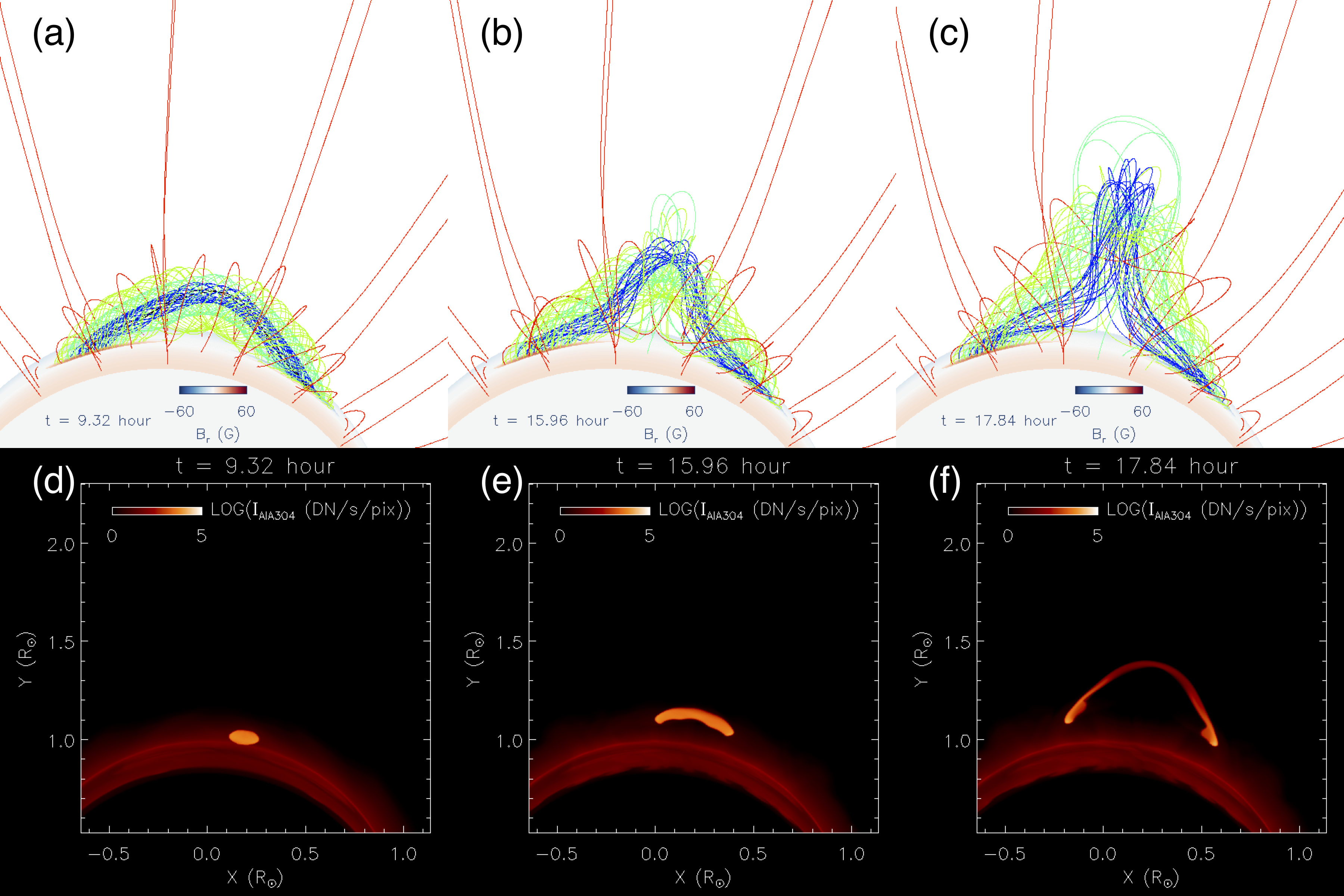
Figure 1: Snapshots of the 3D magnetic field lines viewed from the broad side of the flux rope (upper panels) and the corresponding synthetic SDO/AIA 304 channel emission images (lower panels) showing the prominence condensation carried by the flux rope, produced by the simulation “WS-L” case described in F17. A movie of the evolution is available in the online version of the paper.

The way the SDO/AIA 304 channel emission images are computed is described in F17 (see eq. (23) in that paper). As can be seen from the Figure, the prominence condensation forms in the middle dipped portions of the flux rope field lines. As described in F17, the prominence carrying flux rope undergoes a quasi-static slow rise phase as it develops the kink instability, until roughly $t=17.5$ hr, when it develops a “hernia-like” ejective eruption.

Given the simulation data of the magnetic field, plasma density, temperature, and line of sight velocity, we synthesize the observed Stokes I and V profiles of the forbidden emission line of FeXIII (1074.7nm) by computing and integrating the emission coefficients along individual lines of sight (LOS) through the simulation domain with the CLE code. A line-of-sight (LOS) magnetic field $B_{\rm LOS}$ can be inferred from the observed Stokes V circular polarization profile $V_{\lambda}$ of the emission line assuming the magnetograph formula (e.g. Tomczyk, 2015):

$$V_{\lambda}=-kB_{\rm LOS}\frac{\partial I_{\lambda}}{\partial\lambda},$$ (1)

where $\lambda$ denotes the wavelength, $k=8.1\times 10^{-6}{\rm nm}/{\rm G}$ denotes the Zeeman sensitivity for the FeXIII line at 1074.7 nm, and $I_{\lambda}$ denotes the line intensity profile. Assuming the emission line profile is approximately Gaussian:

$$I_{\lambda}=I_{0}\exp\left(-\frac{(\lambda-\lambda_{0})^{2}}{{\Gamma}^{2}}\right),$$ (2)

where $\lambda_{0}$ is the line-center wavelength (where $I_{\lambda}$ peaks) and $\Gamma$ is the e-folding line width, it can be shown that:

$$B_{\rm LOS}=\frac{\sqrt{\pi}}{2}\frac{\Gamma}{k}\frac{V}{I},$$ (3)

where

$$V=\int V_{\lambda}\,{\rm sgn}(\lambda-\lambda_{0})\,d\lambda$$ (4)

and

$$I=\int I_{\lambda}\,d\lambda$$ (5)

are the wave-length integrated Stokes $V$ and $I$ signals observed. One can estimate an error or uncertainty of the $B_{\rm LOS}$ inferred from the observed $V/I$ signals of the Fe XIII line due to photon noise (Tomczyk, 2015; Lin, 2017):

$$\sigma_{B}=\frac{\sqrt{\pi}}{2}\frac{\Gamma}{k}\frac{1}{\epsilon_{V}\sqrt{\Phi_{I}}}\left(1+2\frac{\Phi_{sc}}{\Phi_{I}}\right)^{1/2}\;({\rm G}),$$ (6)

where $\sigma_{B}$ is the error of $B_{\rm LOS}$, $\Phi_{I}$ denotes the total number of detected photons in the line:

$$\Phi_{I}=1.01\times 10^{6}I_{0}\,\sqrt{\pi}\,\Gamma\,\Delta t\,\epsilon\,(\Delta x)^{2}\,D^{2}\;({\rm photons}),$$ (7)

and $\Phi_{sc}$ is the background scattered light photons over the same wavelength range. In the above $I_{0}$ is the line center intensity in units of parts per million (ppm) of the solar disk center intensity, $\Gamma$ is the observed line width in units of nm, $\Delta t$ is the integration time in seconds, $\epsilon$ is the system efficiency, $\epsilon_{V}$ is the modulation efficiency for Stokes V, $\Delta x$ is the size of the spatial resolution element in arcsec, $D$ is the telescope diameter in meters. $\Phi_{sc}$ is computed the same way as $\Phi_{I}$ but with $I_{0}$ in equation (7) replaced with the background corona brightness in ppm, which we assume to be 5 ppm for the noise estimate. This level of the background coronal brightness is adopted because it is achieved with the COSMO K-Coronagraph (K-Cor) and the Coronal Multi-Channel Polarimeter (CoMP) instruments at the Mauna Loa Solar Observatory (MLSO). We have used $\Delta t=714$ sec (about 12 min), $\epsilon=0.05$, $\epsilon_{V}=1/\sqrt{3}$, $\Delta x=12$ arcsec, $D=1.5$ m for the observation with the COSMO LC. Although the LC has planned to have the capability to observe at a resolution of $\Delta x=2$ arcsec, we here use a larger measurement pixel size of 12 arcsec to gain signal to noise, and to accommodate a reasonably short integration time for detecting the early phase of the onset of eruption, where features begin to move across the pixels more quickly, limiting the allowed integration time. For synthesizing the $V_{\lambda}$ and $I_{\lambda}$ profiles, the LOS integrations are first carried out at the resolution of the simulation domain. The emergent line profiles for the individual plane-of-sky (POS) grid points (at about 2 arcsec resolution) are then averaged over the assumed observation reslution element ($\Delta x=12$ arcsec). These spatially averaged line profiles (at the observation resolution) obtained for the individual simulation snapshots (output at about 3 min intervals) are further averaged over the integration time of about 12 min to obtain the final line profiles $V_{\lambda}$ and $I_{\lambda}$ used to infer $B_{\rm LOS}$ via equations (3), (4), and (5), and $\sigma_{B}$ via equations (6) and (7). We further note that for the LOS integration, we have assumed that the prominence condensations are optically thick, such that when the LOS hits the cool plasma below temperature of $10^{5}$K, we stop the integration beyond that point, assuming the emission from the plasma behind is obscured by the prominence and does not contribute to the final emergent profile.

3 Forward Modeled Results

Figure 2(a) shows a snapshot of the inferred $B_{\rm LOS}$ from the synthesized V and I signals as described in the above section, assuming the simulation domain is centered above the west limb at the equator, with the LOS parallel to the axis of the emerging flux rope. Here the $x$-direction is the LOS direction pointing towards the observer and the y-z plane denotes the plane-of-sky (POS). Panel (b) is the same as (a) but only shows the inferred $B_{\rm LOS}$ for which the signal-to-noise ratio ($|B_{\rm LOS}|/\sigma_{B}$) is above 3. A $3\sigma$ detection is typically considered a significant detection with a 99.87 % confidence that the result is real. For the remainder of the paper, we call such inferred $B_{\rm LOS}$ as the measurable $B_{\rm LOS}$. For comparison, panel (c) shows the LOS component $B_{x}$ of the magnetic field in the plane-of-sky cross-section (which corresponds to the axial field in the mid cross-section of the flux rope), and panel (d) shows the 3D magnetic field lines of the flux rope as viewed from the observer’s perspective.

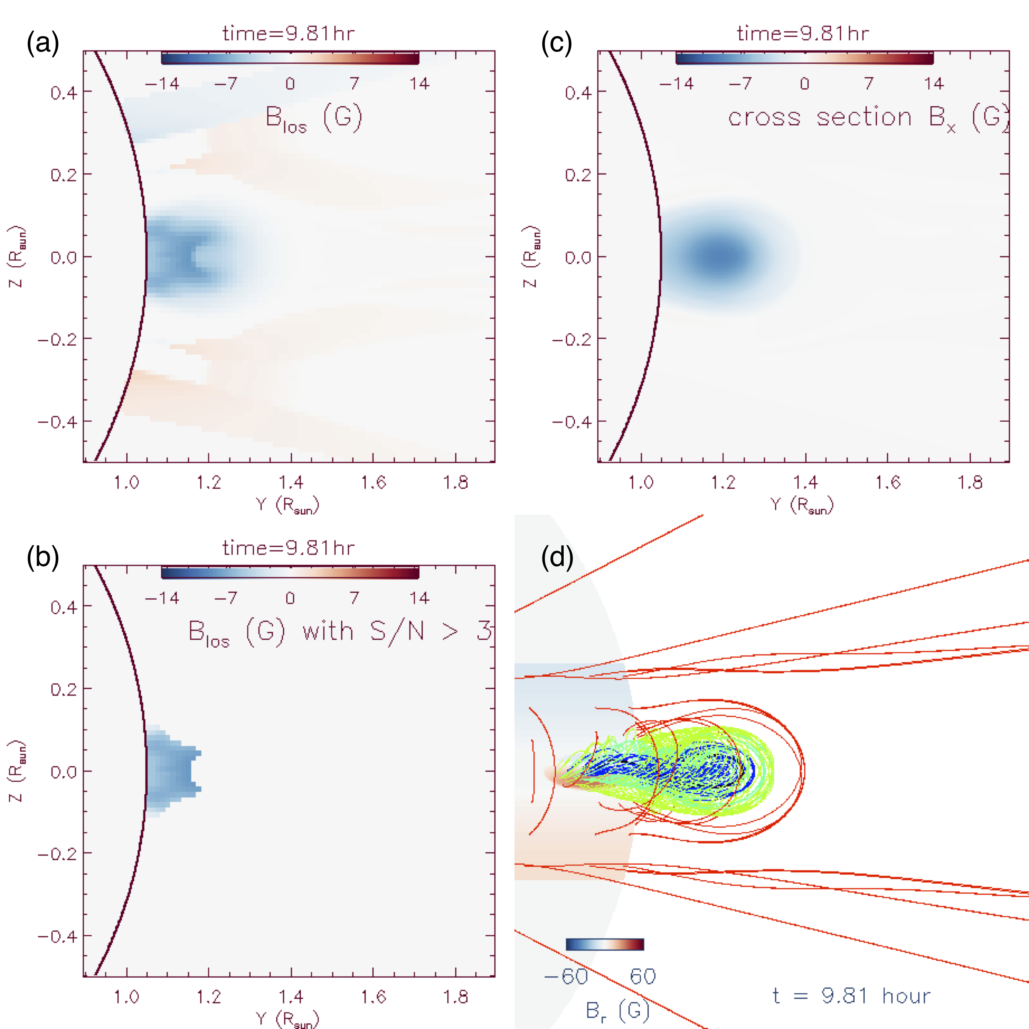
Figure 2: (a) The inferred $B_{\rm LOS}$ (where the $x$-direction is the LOS direction) obtained from the forward synthesis of the MHD model data (as described in Section 2) at a time during the quasi-static phase of the flux rope; (b) The same as (a) but only shows the pixels of the measurable $B_{\rm LOS}$ (see text); (c) The axial field strength in the mid cross-section of the flux rope; (d) The 3D field lines of the coronal magnetic field as viewed from the observer’s perspective, with the LOS parallel to the axis of the emerging flux rope. A corresponding movie showing the evolution of the field strength maps and the 3D flux rope view is available in the online version.

It can be seen from the figure that one can detect a measurable $B_{\rm LOS}$ that is of similar magnitude (peaked at 7.9 G) as the axial field of the flux rope in the mid cross section (peaked at 9.1 G), although the spatial profile of the inferred $B_{\rm LOS}$ in the POS shows significant differences from that of the axial field $B_{x}$ in the mid cross-section (at $x=0$) of the flux rope. To see this more quantitatively, Figure 3 shows the inferred $B_{\rm LOS}$ as a function of height $Y$ along the line near the center at $Z=0.0063R_{\rm sun}$ in the POS map shown in Figure 2(a)) compared with the axial field $B_{x}$ along the same line at $Z=0.0063R_{\rm sun}$ in the mid cross-section of the flux rope shown in Figure 2(c).

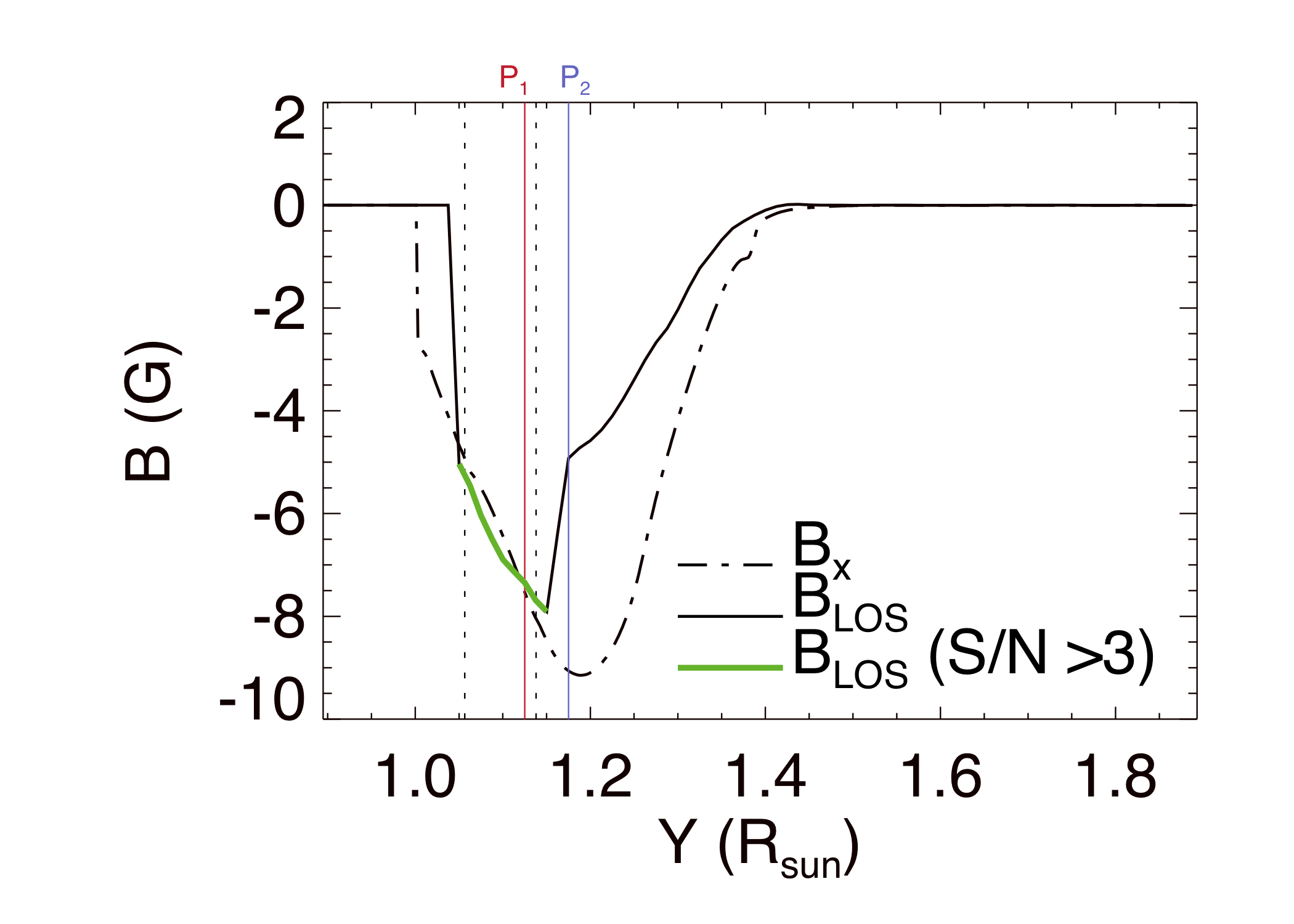
Figure 3: Inferred $B_{\rm LOS}$ (solid line) along the line of $Z=0.0063R_{\rm sun}$ in the POS map shown in Figure 2(a), compared with the axial field $B_{x}$ (dashed-dotted line) along the same $Z=0.0063R_{\rm sun}$ line in the mid cross-section (also the POS cross-section) of the flux rope shown in Figure 2(c).The green solid curve shows the portion of the measurable $B_{\rm LOS}$. The dotted lines bracket the height range of the prominence. The positions $P_{1}$ and $P_{2}$ indicated by the red and blue lines are referred to later when discussing Figure 9.

It can be seen that the two quantities are close for the range from $Y=1.05R_{\rm sun}$ (edge of the COSMO occulting disk) to about $Y=1.14R_{\rm sun}$, which is the height range of the prominence (see Figure 4), above which the magnitude of the inferred $B_{\rm LOS}$ becomes significantly smaller than that of $B_{x}$.

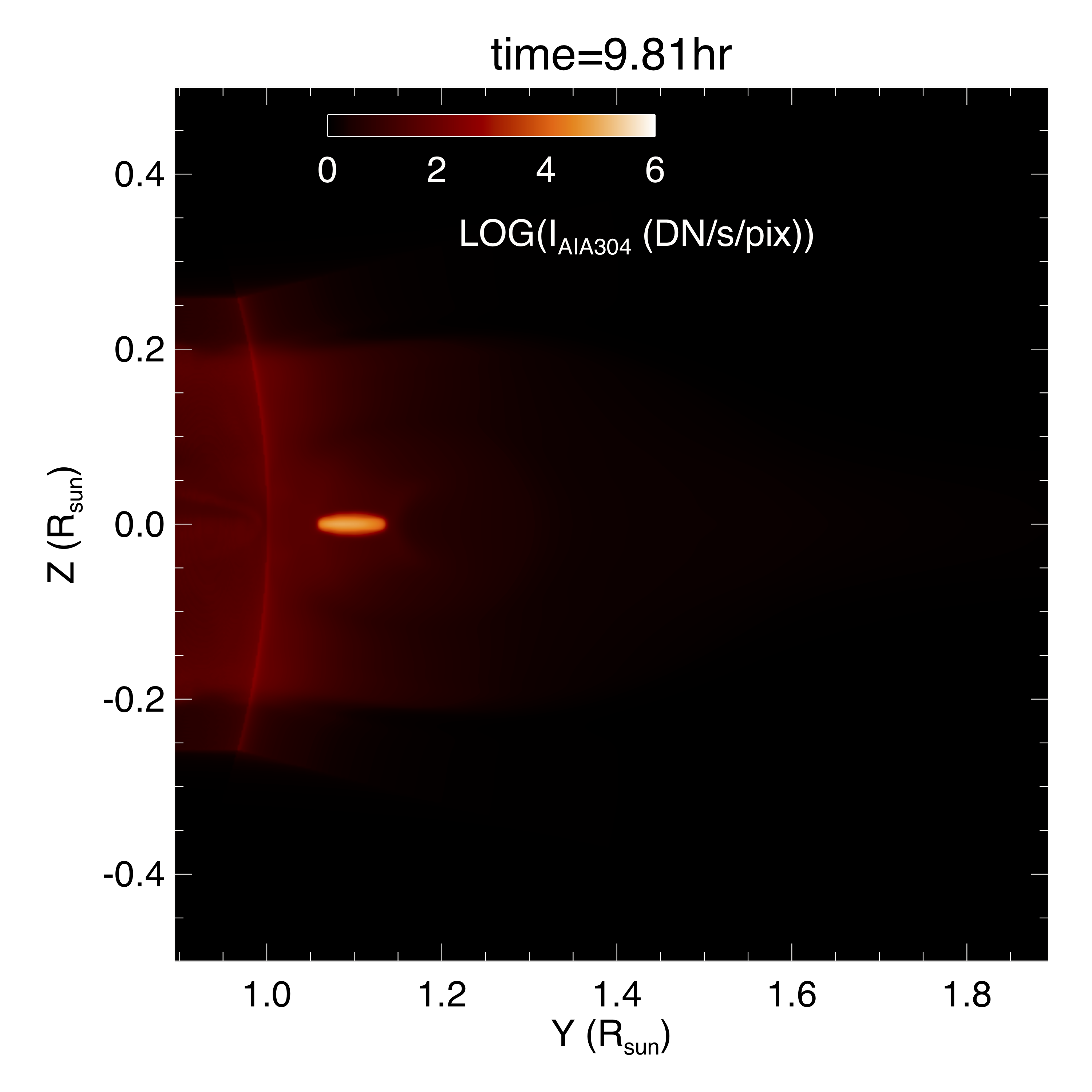
Figure 4: Synthetic SDO/AIA 304 Å channel emission from the same viewing direction as that for the flux rope shown in Figure 2(d) at the same time instant.

Figure 5 shows the relative difference between the measureable $B_{\rm LOS}$ in the POS (Figure 2(b)) and the axial field strength $B_{x}$ in the flux rope mid cross section (Figure 2(c)). It can be seen that the difference is small (less than 10%) over the region around the central prominence. There are two regions further away from the prominence (see the two blue blobs in the image), where the measured $B_{\rm LOS}$ is significantly higher in magnitude (by about 90%) than the $B_{x}$ because the LOSs in these regions intersect the strong fields in the legs of the flux rope in front of and behind the POS.

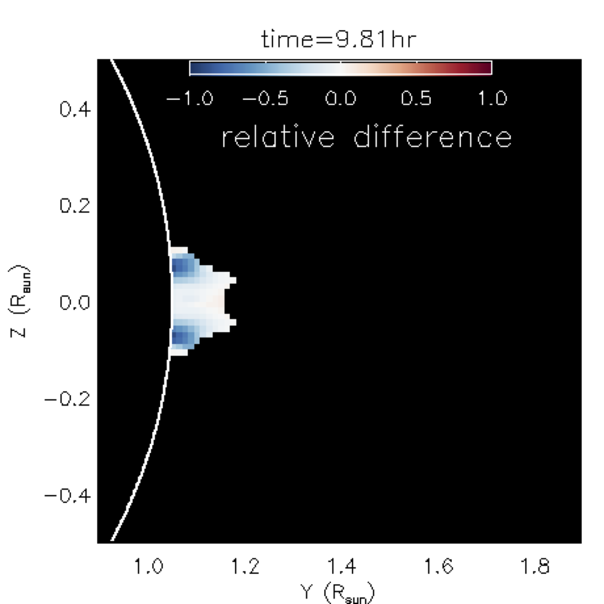
Figure 5: Relative difference, $(B_{\rm LOS}-B_{x})/|B_{x}|$, between the measurable $B_{\rm LOS}$ shown in Figure 2(b) and the $B_{x}$ in the flux rope mid cross section shown in Figure 2(c).

As given in equation (3), the inferred $B_{\rm LOS}$ is directly proportional to the synthetic V/I (shown in Figure 6),

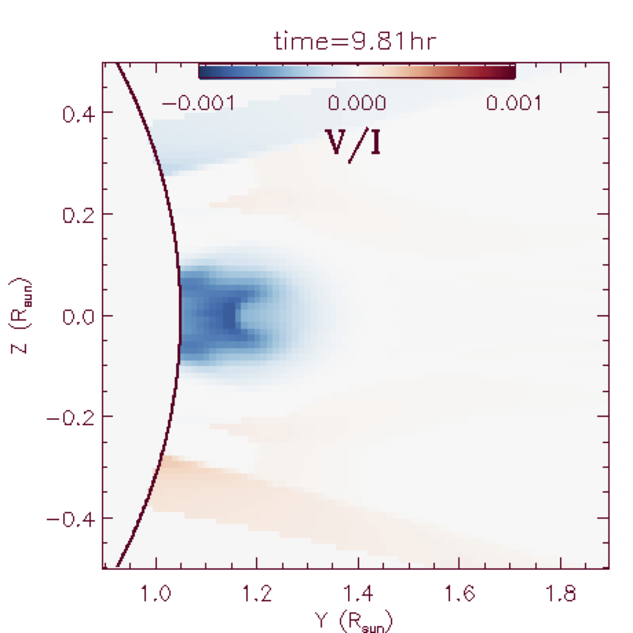
Figure 6: The synthetic V/I signal corresponding to the same time instance shown in Figure 2.

with the proportionality factor varying with the line width $\Gamma$. The synthetic V/I reaches a peak magnitude of about 0.001 here for our modeled flux rope with $\sim 10$ G peak axial field strength. As described in section 2, the V and I signals are given by the synthesized Stokes V and I profiles of the FeXIII emission line through LOS integrations with the CLE code. Thus the inferred $B_{\rm LOS}$ is approximately an FeXIII line intensity weighted mean of the LOS component $B_{x}$ of the magnetic field along the LOS that goes through different parts of the flux rope. To see the temperature sensitivity of the the FeXIII line, we show in Figure 7 the line center intensity ($f_{I_{0}}$) obtained from a LOS integration with the CLE code assuming constant plasma properties (temperature, electron density and magnetic field) along the LOS, as a function of the (constant) temperature (T) value used for the LOS while keeping the other plasma parameters fixed.

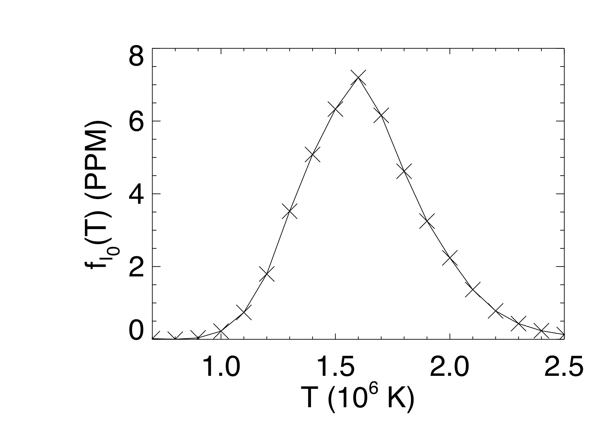
Figure 7: The line center intensity ($f_{I_{0}}$) obtained from a LOS integration with the CLE code assuming constant plasma properties (temperature, electron density and magnetic field) along the LOS, as a function of the temperature (T) value used for the LOS, while keeping the other plasma parameters fixed (assuming electron density of $10^{8}{\rm cm}^{-3}$, and a constant magnetic field of 1G along the line of sight).

It shows that the FeXIII line has a fairly narrow temperature sensitivity, which peaks at about $T=1.6$ MK, but reduces by an order of magnitude when $T$ rises to about $2.2$ MK or decreases to about $1.1$ MK. The CLE code models the line emission under the combined influence of resonance scattering and particle collisions. The line intensity shows a dependence on electron density $N_{e}$ that is between linear and quadratic (e.g. Gibson et al., 2016). Assuming that the FeXIII line intensity is approximately proportional to $f_{I_{0}}(T)\,N_{e}$, we have computed a weighted-mean $B_{\rm LOS}$ over each LOS: $\int B_{x}\,W(x)\,dx/\int W(x)\,dx$, where $W(x)\propto f_{I_{0}}(T(x))N_{e}(x)$ and x is the coordinate along the LOS direction. The resulting weighted-mean $B_{\rm LOS}$ in the POS is shown in Figure 8.

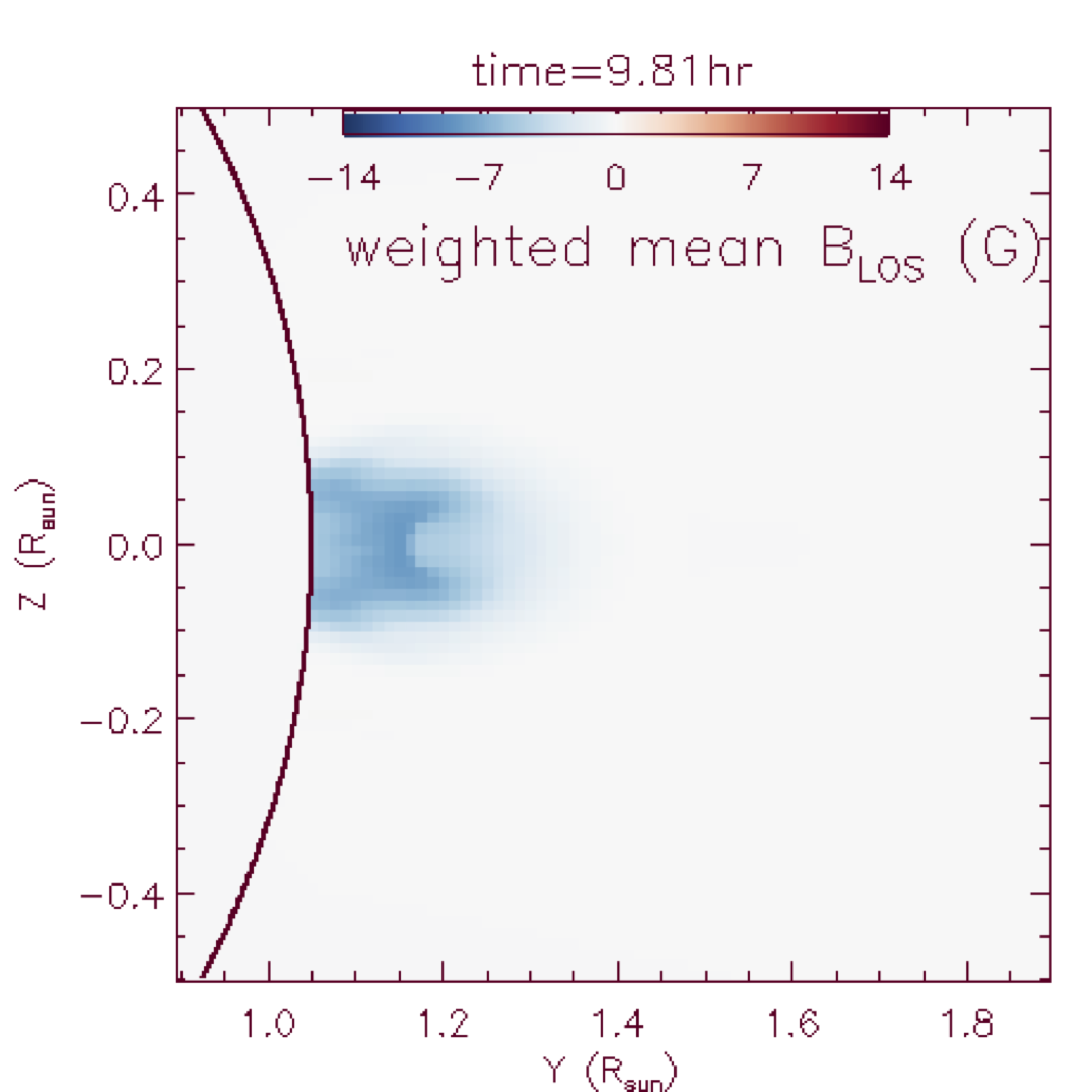
Figure 8: POS map of the weighted-mean $B_{\rm LOS}$ over each LOS (see text for how the weighted mean is computed).

It is in good agreement with the inferred $B_{\rm LOS}$ shown in Figure 2(a) obtained from the synthesized V and I profiles from the CLE code, in the region of the flux rope. Thus $W(x)$ gives a good approximation of the relative weight each part of the LOS contributes to the inferred $B_{\rm LOS}$. Figure 9 shows the profiles of various quantities along two example LOSs from which the $B_{\rm LOS}$ at the $P_{1}$ and $P_{2}$ positions (marked by the red and blue lines) in Figure 3 are obtained.

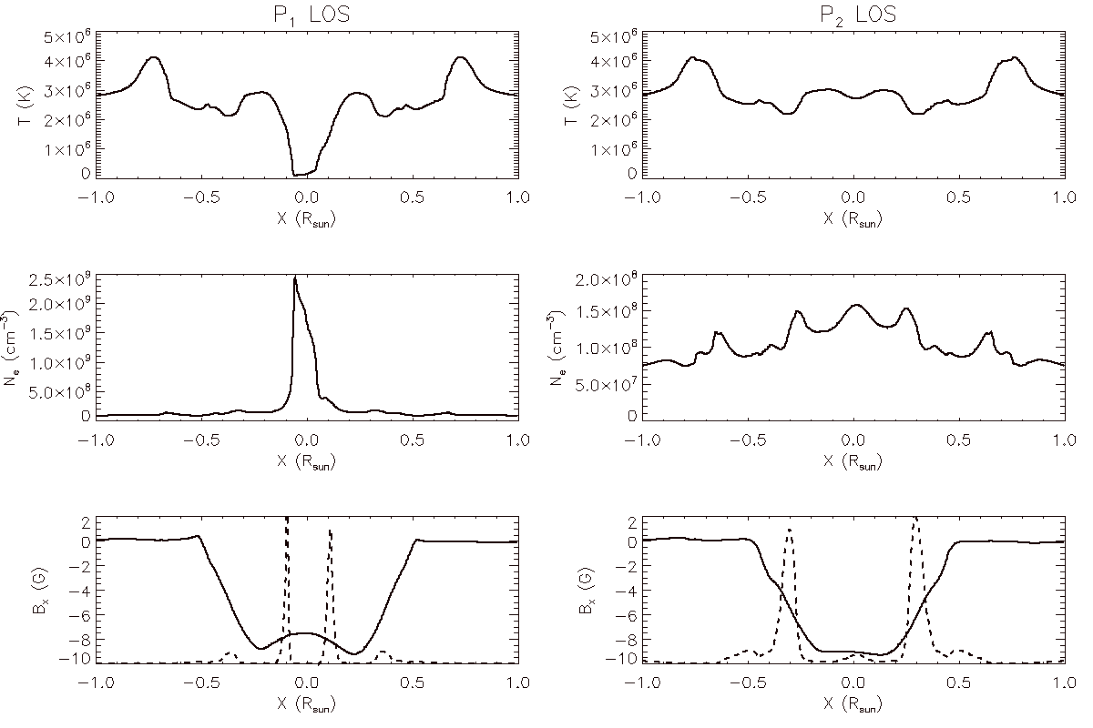
Figure 9: Profiles of temperature T, electron density $N_{e}$, LOS field strength $B_{x}$, along two example LOSs (left and right columns). The left (right) column shows the LOS that produces the inferred $B_{\rm LOS}$ at $P_{1}$ ($P_{2}$) marked by the red (blue) line position in Figure 3. The $P_{1}$ and $P_{2}$ LOSs correspond to the POS positions of ($Y=1.127R_{\rm sun}$, $Z=0.0063R_{\rm sun}$) and ($Y=1.177R_{\rm sun}$, $Z=0.0063R_{\rm sun}$) respectively in Figures 2(a)(b). The dashed line in the bottom panels shows the variation of the weight function $W(x)\propto f_{I_{0}}(T(x))N_{e}(x)$ along the LOS (x), in relation to the variation of $B_{x}$ along the LOS.

For the $P_{1}$ LOS profiles shown in the left column panels, the LOS approaches the prominence at the middle (x=0) of the LOS. The estimated weighting function $W(x)$ (dashed line) along the LOS has two narrow peaks just outside the prominence condensation, where T transitions steeply from below $10^{5}$ K to the hot “cavity” temperature of above 2 MK, going through the peak sensitivity temperature of 1.6 MK. Thus the inferred $B_{\rm LOS}$ is sampling the prominence carrying field lines at the positions of prominence-to-cavity transition (further illustration with Figure 12 below), and is fairly close to the axial field strength $B_{x}$ at $x=0$ for the $P_{1}$ LOS (see bottom left panel of Figure 9). Note for this LOS, because of the optically thick assumption for the prominence condensations, only the part along the LOS from $x=1$ to $x=-0.07$ contributes to the LOS integration for synthesizing the stokes profiles with the CLE code and also for evaluating the weighted mean $B_{\rm LOS}$ shown in Figure 8. We find that for all the LOSs that intersect the prominence vicinity, because of the sampling property described above, the inferred $B_{\rm LOS}$ is close to the axial field $B_{x}$ at the central prominence dip at that height (see the height range of $Y=1.05R_{\rm sun}$ to $1.14R_{\rm sun}$ in Figure 3). Thus over this height range, the inferred $B_{\rm LOS}$ can discern (with sufficient signal to noise ratio) the increase with height of the field strength of the prominence carrying field lines, which is an indication that field lines are dipped (e.g. F17, section 1.8 in Priest, 2014). On the other hand, for the higher LOS at $P_{2}$ (see right column panels of Figure 9), the LOS is intersecting the hot core of the flux rope above the prominence, with $T\approx 3$ MK around $x=0$ on the LOS, where $B_{x}$ is the strongest. The peak sampling represented by $W(x)$ (dashed line) is outside of the peak core field of the flux rope (bottom right panel of Figure 9), in the region where the temperature is relatively lower outside of the central hot core (top right panel of Figure 9). Thus the resulting inferred $B_{\rm LOS}$ is significantly lower than the mid cross-section axial field $B_{x}$ at the $P_{2}$ height as seen in Figure 3. Furthermore, because the temperature along the entire LOS for $P_{2}$ is high, out of the sensitive range of the FeXIII line, the line intensity obtained for this LOS is a factor of 10 smaller than that of the $P_{1}$ LOS. The resulting inferred $B_{\rm LOS}$ at $P_{2}$ is thus below the error estimated from the photon noise, and thus not in the measurable $B_{\rm LOS}$ map in Figure 2(b).

Figure 10 shows the measurable $B_{\rm LOS}$ (left panels) for two other viewing angles, where the flux rope centered above the limb (see the right panels for the 3D views in Figure 2) is rotated from the azimuthal direction by $7^{\circ}$ anti-clockwise (upper panels) and clockwise (lower panels) respectively.

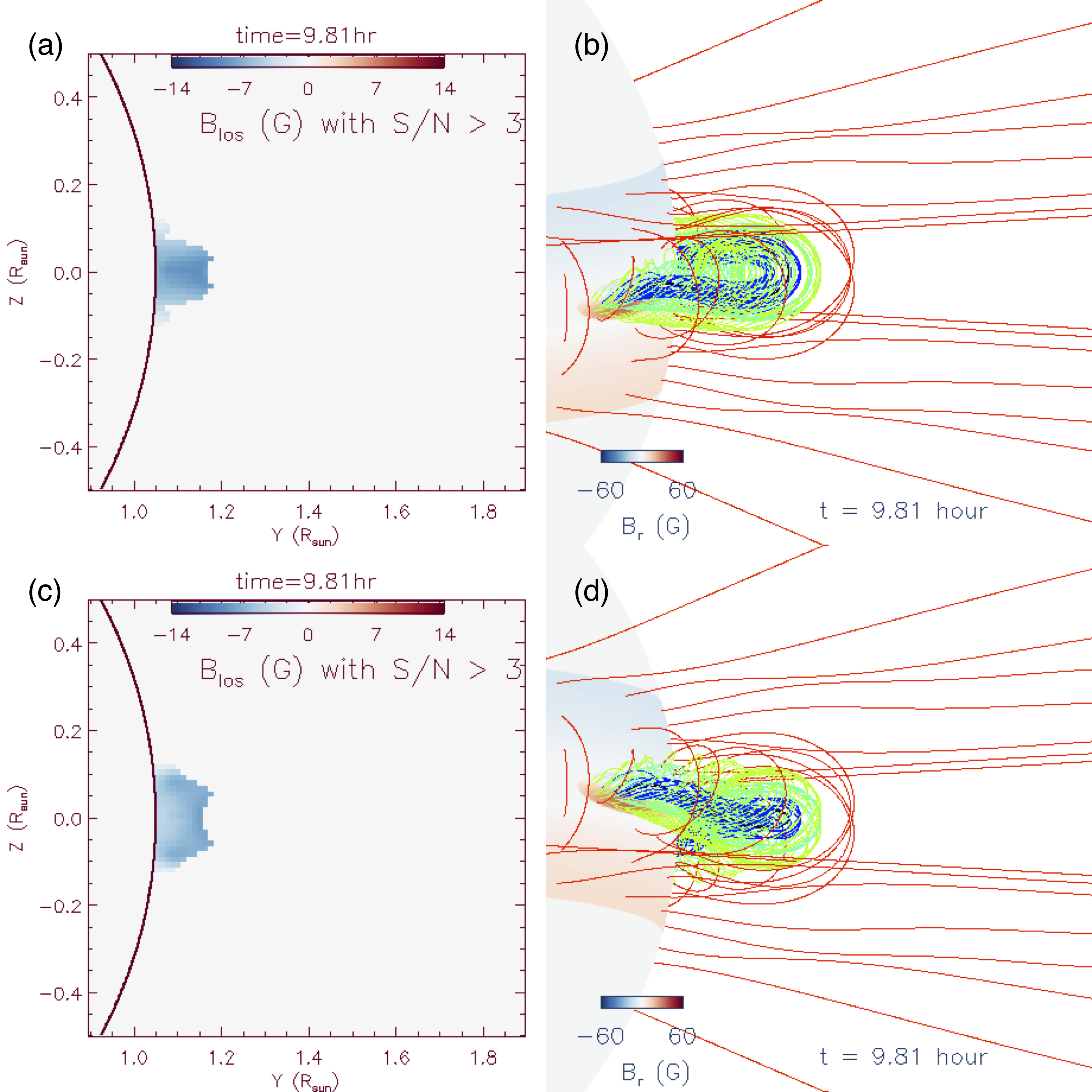
Figure 10: The measurable $B_{\rm LOS}$ (left panels) obtained from the forward synthesis of the MHD model data (as described in Section 2) for two different viewing angles as illustrated by the 3D field line plots (right panels), with the flux rope centered above the limb as in Figure 2 but rotated from the azimuthal direction by $7^{\circ}$ anti-clockwise (upper panels) and clockwise (lower panels) respectively at the same time instant during the quasi-static phase of the flux rope.

For both viewing angles, one can measure a significant $B_{\rm LOS}$ (with a peak value of 8.4 G and 7.4 G respectively) in the flux rope region in the POS over the height range of the prominence, similar to the results for the previous viewing angle shown in Figure 2(b)(d). In all three cases (see the POS maps in Figure 2(b) and Figures 10(a)(c)), the measurable $B_{\rm LOS}$ shows an increase with height (Y) in the central region near $Z=0$ (near the prominence). This is shown more quantitatively by the green solid curves in Figure 11 and Figure 3, which show the profiles of the measurable $B_{\rm LOS}$ along the line of $Z=0.0063R_{\rm sun}$ in the POS maps. The prominence height range is between the dotted lines.

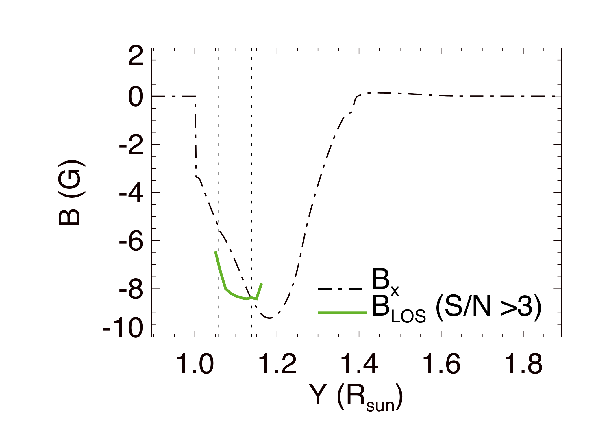
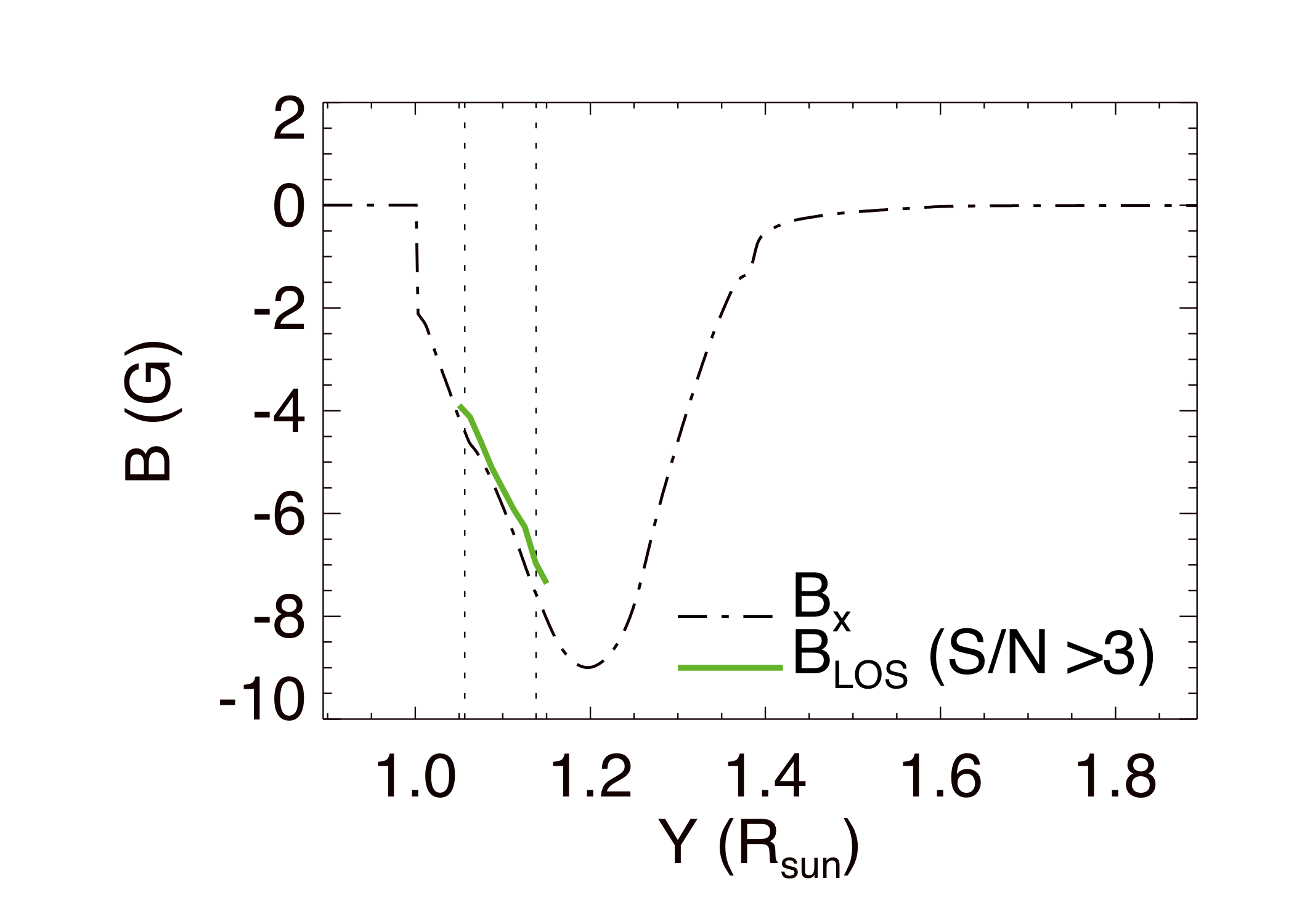
Figure 11: Profile of the measurable $B_{\rm LOS}$ (green curves) as a function of height $Y$ along the line of $Z=0.0063R_{\rm sun}$ in the POS map shown in Figure 10(a) (upper panel) and the POS map shown in Figure 10(c) (lower panel). For comparison the LOS field $B_{x}$ along the same line of $Z=0.0063R_{\rm sun}$ in the POS cross-section of the flux rope is shown as the dash-dotted lines.

The measurable $B_{\rm LOS}$ profiles all show increase with height over the prominence height range and their values are fairly close to the LOS field strengths of the flux rope in the mid cross-section.

The reason for this is further illustrated in Figure 12.

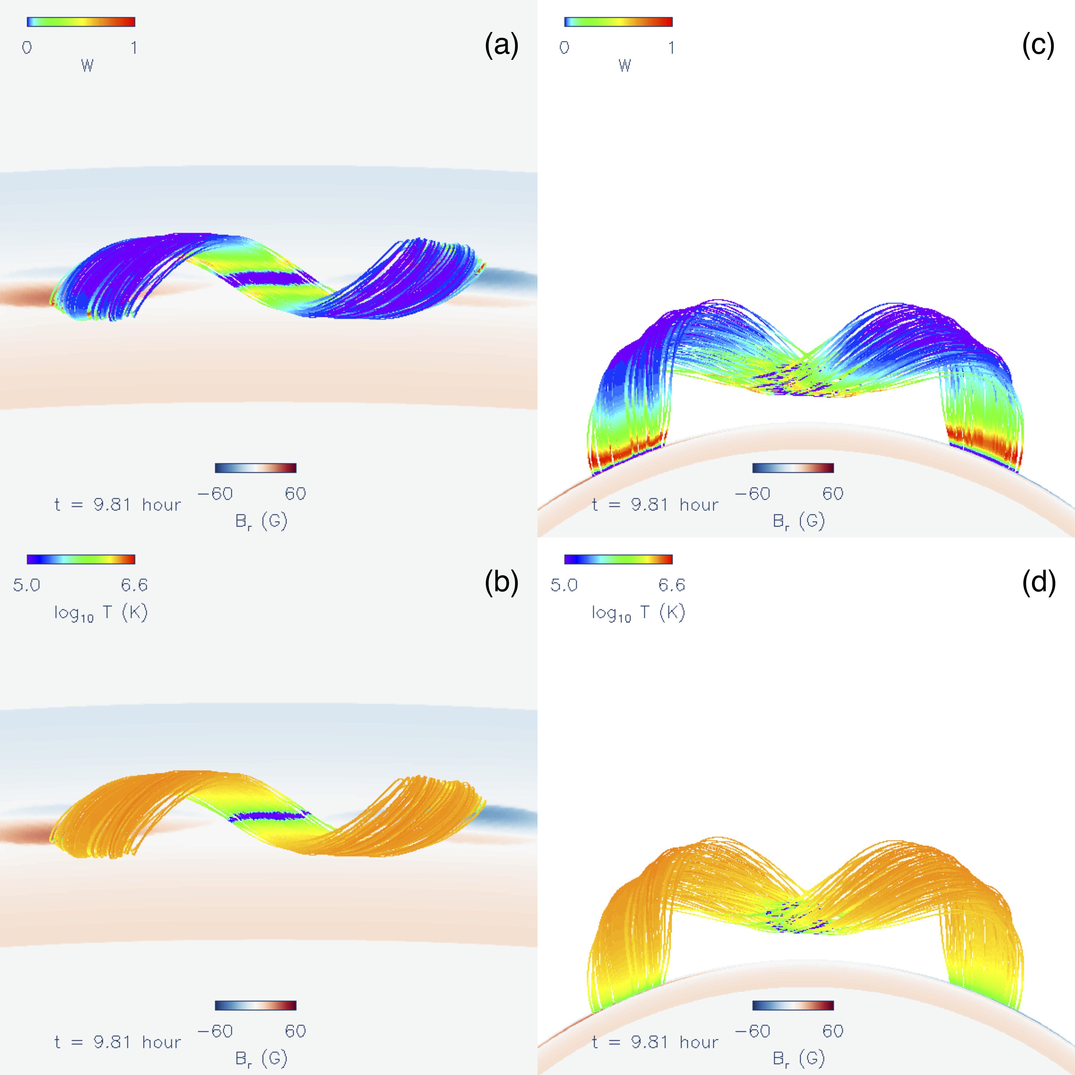
Figure 12: 3D views of the densely traced prominence carrying field lines colored based on the weighting function $W\propto f_{I_{0}}(T)N_{e}$ (top panels), and corresponding views of the field lines colored based on the temperature (bottom panels)

The top panels show 3D views of the densely traced prominence carrying field lines colored with the weighting function $W\propto f_{I_{0}}(T)N_{e}$, showing which parts of the field lines contribute strongly (with higher $W$) to the FeXIII emission and hence to the $B_{\rm LOS}$ measurement. For reference the temperature distribution along the prominence field lines are shown in the lower panels of Figure 12. It can be seen that the parts that the $B_{\rm LOS}$ measurement is sensitive to are just outside of the central prominence condensations, at the transition from prominence temperature to the hot cavity temperature along the prominence carrying field lines. This further illustrates that the measured $B_{\rm LOS}$ for the prominence height range tends to be fairly close to the field strength at the prominence dip and reflects its variation (increase) with height. We emphasize that this localization of the measured field strength is because of the specific temperature configuration in the simulation that the signal comes mostly from around the cold prominence. If the temperature distribution in the flux rope outside of the prominence is more uniformly close to the 1.6 MK formation temperature of the FeXIII line, then the measured field strength would not reflect so closely the field strength of the prominence dips, as we will show later in a different case at the end of this section.

Figure 13 shows the POS maps of the measurable $B_{\rm LOS}$ and the 3D flux rope viewed from the corresponding observation perspectives at a later time instance towards the end of the slow rise phase, just before the onset of eruption.

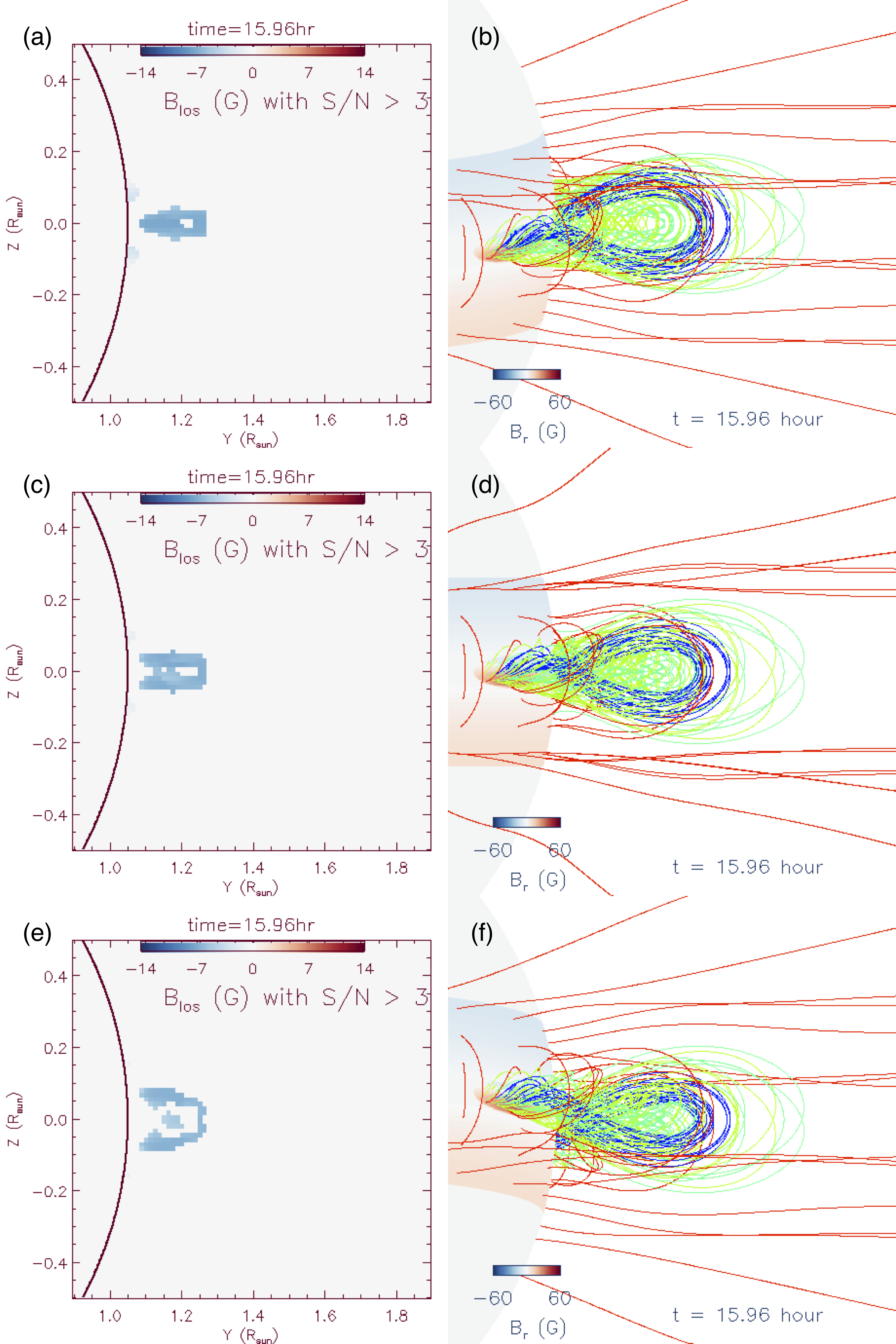
Figure 13: The top, middle, and bottom rows are the same as Figures 10(a)(b), Figures 2(b)(d), and Figures 10(c)(d) respectively, except at a later time instance towards the end of the slow rise phase. A corresponding movie of the evolution of the measurable $B_{\rm LOS}$ maps and the flux rope views is also available in the online version.

It corresponds to the time instance shown in Figure 1(b)(e), where the flux rope has become significantly kinked and the prominence is rising. A movie of the evolution of the $B_{\rm LOS}$ maps and the flux rope views corresponding to Figure 13 is also available in the online version. We can see from the Figure and the movie that we can detect a measurable out-moving $B_{\rm LOS}$ through the slow rise phase up to a height of about $y=1.3R_{\rm sun}$, and until a time when the flux rope has accelerated to a speed of about $41$ km/s. After that, we no longer detect a measurable outward moving field.

There are significant uncertainties in regard to the plasma thermodynamic properties obtained in the simulation, for which a highly simplified coronal heating is assumed. We therefore have considered an alternative extreme case where we replace the plasma properties (temperature, density, and velocity) in the simulation domain with a hydrostatic isothermal atmosphere with $T=1.6$ MK (at maximum sensitivity of the FeXIII line) and a base density of $5\times 10^{8}{\rm cm}^{-3}$, only keeping the simulated magnetic field evolution for the forward modeling to see how much the resulting inference of the $B_{\rm LOS}$ can differ. The results for the inferred and measurable $B_{\rm LOS}$ for the same observation view as that of Figure 2 are shown in Figure 14.

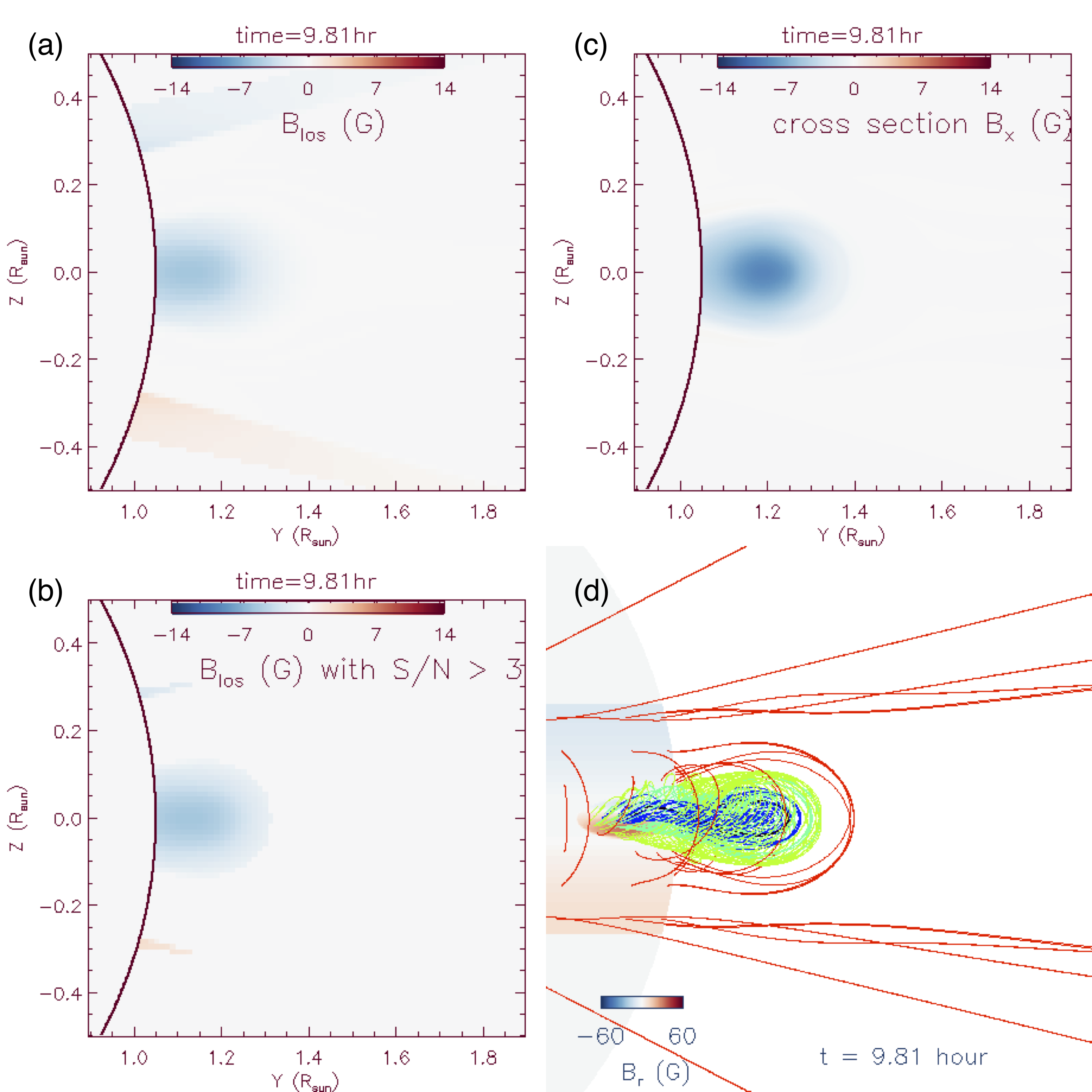
Figure 14: Same as Figure 2 except using the hysrostatic isothermal corona at 1.6 MK to replace the plasma properties in the simulation domain.

Comparing this to Figure 2, we find that the measurement sensitivity is significantly increased such that the observation can now measure a significant $B_{\rm LOS}$ nearly throughout the flux rope cross section in the POS (Figure 14(b)), although the magnitude of the measured field strength significantly under estimates the axial field strength $B_{x}$ in the mid cross section of the flux rope (Figure 14(c)). Figure 15 shows a quantitative comparison of the field strength profiles along the central slice at $Z=0.0063R_{\rm sun}$ in the POS.

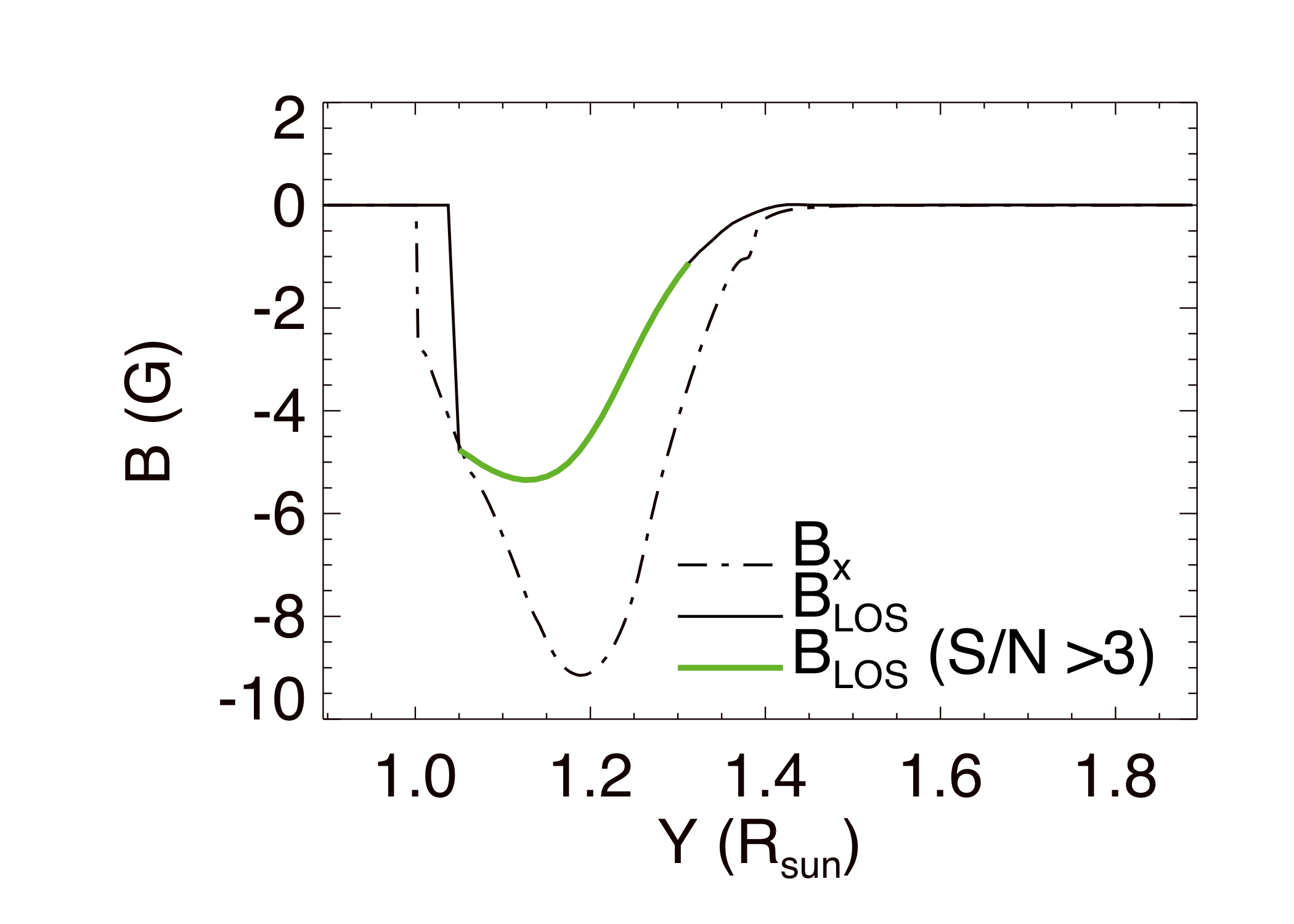
Figure 15: Same as Figure 3 except for the case with the hysrostatic isothermal corona at 1.6 MK replacing the plasma properties in the simulation domain.

The measured peak field strength of $B_{\rm LOS}$ is roughly a half of the peak axial field strength $B_{x}$ of the flux rope. The under estimate of the flux rope field strength by the measured $B_{\rm LOS}$ is due to the broad averaging along the LOSs with much more uniform weighting (because of the uniform temperature and smoother density variation) through the flux rope and the outside arcade field where the $B_{\rm LOS}$ component is weak. Nevertheless, the measured $B_{\rm LOS}$ still shows a region of (weaker) increase of field strengt with height in the lower height range of the flux rope cross section, indicative of the concave upturning field geometry of the flux rope there. Figure 16 shows the measured $B_{\rm LOS}$ in the POS at a later time when the flux rope has begun to erupt, and a movie corresponding to the Figure showing the temporal evolution of the measured $B_{\rm LOS}$.

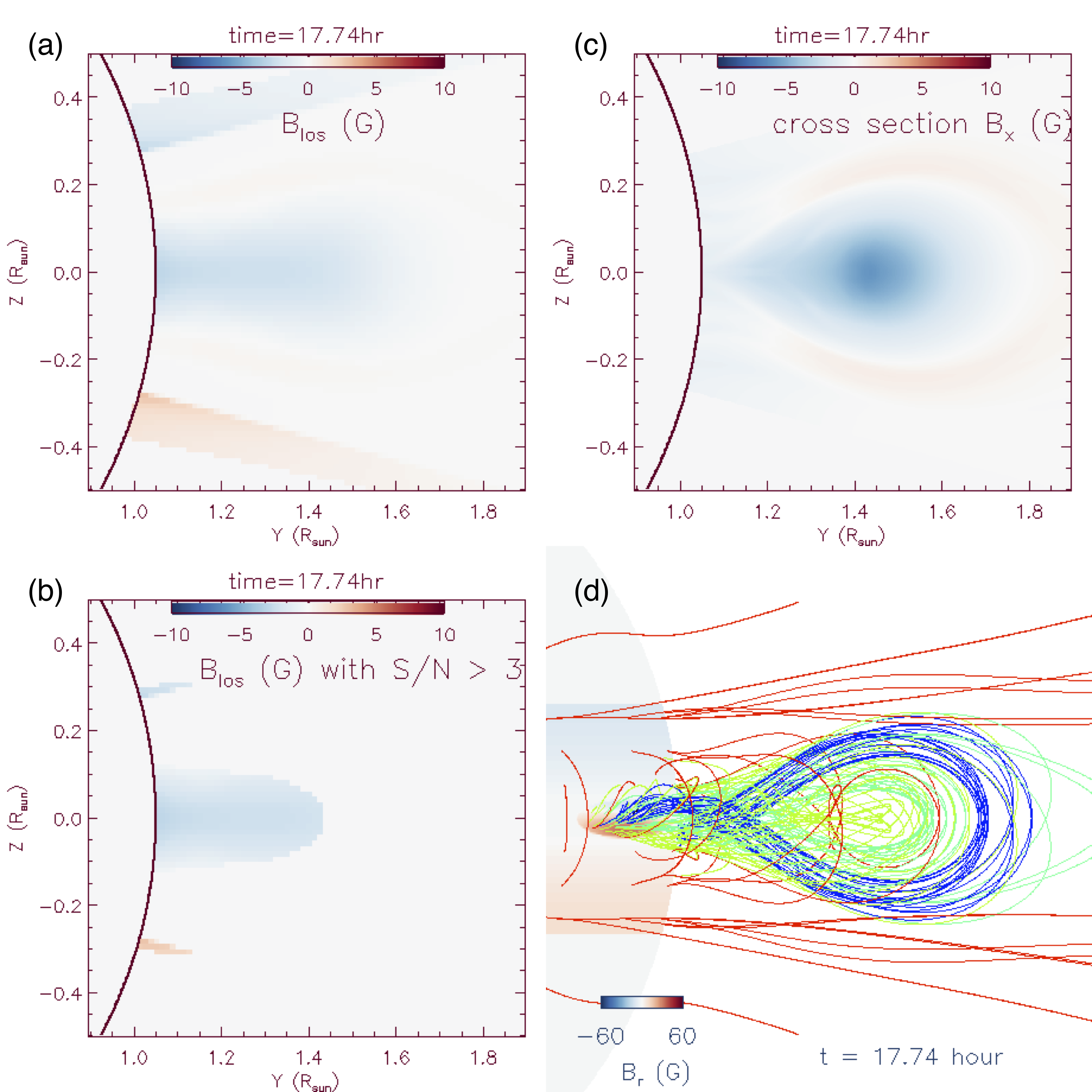
Figure 16: Same as Figure 14 except for a later time at $t=17.74$ hr when the flux rope has begun to erupt, and also the change in the color table range for the field strength. A corresponding movie showing the evolution of the magnetic field is also available in the online version.

We find that in this case we can detect a measurable outgoing $B_{\rm LOS}$ to a greater height (about $1.43R_{\rm sun}$) and over a significantly larger area of the rising flux rope cross section, until a time when the flux rope has accelerated to a speed of $485$ km/s.

4 Discussion and Conclusion

Using an MHD simulation of a prominence carrying coronal flux rope, we have carried out forward synthesis of the circular polarization measurement by the proposed COSMO LC to examine its capability of inferring the LOS magnetic field of the flux rope above the limb, viewed nearly along the length of the flux rope. We found that using an integration time of about 12 min and an observational resolution of 12 arcsec, the LC can measure with sufficient signal to noise ratio ($>3$) the flux rope field strength of a few G in the region around the prominence, within the height range of the prominence. We find that the inferred $B_{\rm LOS}$ can be fairly well approximated by a mean of the LOS component of ${\bf B}$ along the LOS with a weighting that is proportional to $f_{I_{0}}(T)N_{e}$, where $f_{I_{0}}(T)$ describes the temperature sensitivity of the FeXIII line intensity as shown in Figure 7, with a narrow peak at $1.6$MK. Because of this and the temperature configuration of the simulated flux rope, we find that for those LOS that intersect the prominence vicinity, the measured $B_{\rm LOS}$ is localized to the region of prominence-to-hot-cavity transition and is fairly close to the axial field strength at the prominence dip. As a result the measurable $B_{\rm LOS}$ shows fairly accurately its increase with height profile, which is a signature of the concave upturning dipped field lines supporting the prominence.

Above the prominence heights, the flux rope develops a hot core which reaches a peak temperature of about $3$ MK in our MHD model. As a result the LOSs at these heights tend to sample the field strength outside of the hot core strong field region (e.g. the P2 LOS shown in right column of Figure 9), and the inferred $B_{\rm LOS}$ is significantly below the axial field at the corresponding height in the mid cross section of the flux rope, and also does not have enough signal to noise ratio to make it measurable. It is likely that our MHD model is over-estimating the temperature in the hot cavity in the flux rope surrounding the prominence condensation due to the simplified empirical coronal heating used and also due to the heating from the numerical diffusion of the magnetic field. This may have unrealistically reduced the sensitivity of the FeXIII emission line measurement for the flux rope cavity region. We have therefore also examined a case where we have replaced the plasma properties in the simulation domain with a hydrostatic isothermal atmosphere at the peak sensitivity temperature of 1.6 MK for the FeXIII line. In that case we found that the measurement sensitivity is greatly improved such that a significant $B_{\rm LOS}$ can be measured throughout the flux rope cross section in the POS. Although the magnitude of the measured field significantly under estimates the axial field strength of the flux rope because of the broad averaging along the LOS, nevertheless it still detects an increase with height profile in the lower height range, indicating the concave up turning field geometry of the flux rope there. On the other hand X-ray observation of a filament cavity by Hudson et al. (1999) and eclipse observations by Habbal et al. (2010) have indicated high temperatures, of about 2 MK or even higher, for the cavity regions surrounding the prominences. Thus it may be difficult to measure magnetic field strength in the hot cavity region of the flux rope far away from the prominence itself with the FeXIII line. However, our forward analysis shows that it is feasible to measure the field strength in the vicinity of the prominence with the signal from the region of prominence-to-cavity transition as discussed above. This provides important information about the properties of the prominence carrying magnetic fields.

Furthermore, we find that the synthetic observation can measure the outward moving magnetic field around the rising prominence during the slow rise phase as the flux rope develops the kink instability (F17). It can detect the outward moving field up to a height of about $1.3R_{\rm sun}$, until a time when the flux rope accelerates to about $41$ km/s, after which it can no longer detect a measurable field because of the rapid change and the weakening of the field strength. Thus our synthetic observation can track the field strength evolution of the prominence supporting field into its early phase of the onset of eruption. Examination of the extreme case with the isothermal atmosphere with 1.6 MK shows a greatly improved sensitivity in measuring the outward moving field during the onset of the eruption. It can detect a measurable outgoing $B_{\rm LOS}$ over a larger area of the rising flux rope cross section (Figure 16), to a greater height of about $1.43R_{\rm sun}$ and until a time when the flux rope has accelerated to a speed of $485$ km/s. A further improved approach that combines measurements of multiple coronal emission lines, with different temperature sensitivities, might allow a more comprehensive picture of the magnetic field throughout the multi-thermal prominence-cavity system. We leave this for a future study.

References

- Casini & Judge (1999) Casini, R., & Judge, P. G. 1999, ApJ, 522, 524
- Fan (2017) Fan, Y. 2017, ApJ, 844, 26
- Gibson (2015) Gibson, S. 2015, in Astrophysics and Space Science Library, Vol. 415, Solar Prominences, ed. J.-C. Vial & O. Engvold, 323
- Gibson et al. (2016) Gibson, S., Kucera, T., White, S., et al. 2016, Frontiers in Astronomy and Space Sciences, 3, 8
- Gibson (2018) Gibson, S. 2018, Living Reviews in Solar Physics, submitted
- Habbal et al. (2010) Habbal, S. R., Druckmüller, M., Morgan, H., et al. 2010, ApJ, 719, 1362
- Hudson et al. (1999) Hudson, H. S., Acton, L. W., Harvey, K. L., & McKenzie, D. E. 1999, ApJ, 513, L83
- Judge & Casini (2001) Judge, P. G., & Casini, R. 2001, in Astronomical Society of the Pacific Conference Series, Vol. 236, Advanced Solar Polarimetry – Theory, Observation, and Instrumentation, ed. M. Sigwarth, 503
- Judge et al. (2006) Judge, P. G., Low, B. C., & Casini, R. 2006, ApJ, 651, 1229
- Lin (2017) Lin, H. 2017, On the Sensitivity and Measurement Error of SpectroPolarimetry for the Measurement of Coronal Magnetic Fields (private communication)
- Lin et al. (2000) Lin, H., Penn, M. J., & Tomczyk, S. 2000, ApJ, 541, L83
- Priest (2014) Priest, E. 2014, Magnetohydrodynamics of the Sun (Cambridge, UK: Cambridge University Press)
- Tomczyk (2015) Tomczyk, S. 2015, COSMO LC PDR Technical Notes 1, http://mlso.hao.ucar.edu/COSMO/Sections/Technical%20Note%20Series/TN%2001%20Measurement%20Errors.pdf
- Tomczyk et al. (2016) Tomczyk, S., Landi, E., Burkepile, J. T., et al. 2016, Journal of Geophysical Research (Space Physics), 121, 7470
- Webb & Hundhausen (1987) Webb, D. F., & Hundhausen, A. J. 1987, Sol. Phys., 108, 383