Multi-frequency study of the gamma-ray flaring BL Lac object PKS 2233$-$148 in 2009–2012

Abstract

We study the jet physics of the BL Lac object PKS 2233$-$148 making use of synergy of observational data sets in the radio and $\gamma$-ray energy domains. The four-epoch multi-frequency (4–43 GHz) VLBA observations focused on the parsec-scale jet were triggered by a flare in $\gamma$-rays registered by the Fermi-LAT on April 23, 2010. We also used 15 GHz data from the OVRO 40-m telescope and MOJAVE VLBA monitoring programs. Jet shape of the source is found to be conical on scales probed by the VLBA observations setting a lower limit of about 0.1 on its unknown redshift. Nuclear opacity is dominated by synchrotron self-absorption, with a wavelength-dependent core shift $r_{\text{core\,[mas]}}\approx 0.1\lambda_{[\text{cm}]}$ co-aligned with the innermost jet direction. The turnover frequency of the synchrotron spectrum of the VLBI core shifts towards lower frequencies as the flare propagates down the jet, and the speed of this propagation is significantly higher, about 1.2 mas yr^-1, comparing to results from traditional kinematics based on tracking bright jet features. We have found indications that the $\gamma$-ray production zone in the source is located at large distances, 10–20 pc, from a central engine, and could be associated with the stationary jet features. These findings favour synchrotron self-Compton, possibly in a combination with external Compton scattering by infrared seed photons from a slow sheath of the jet, as a dominant high-energy emission mechanism of the source.

1 Introduction

The location of the $\gamma$-ray production zone in active galactic nuclei (AGN) is still an open and actively debated question. Due to a limited angular resolution of the $\gamma$-ray telescopes it is impossible to directly locate the region responsible for the high-energy emission in AGN. A variaty of approaches has been considered to address this problem, and our current understanding is that the regions of $\gamma$-ray production may be at different locations in different sources as evident from observations. One of the two main competing scenarios is based on the observed rapid $\gamma$-ray variability on time scales of a few hours and suggests that the high-energy emission from blazars is generated on sub-pc scales, near the central black hole (e.g., Tavecchio et al., 2010; Yan et al., 2018). Similarly, the observed strength and variability of the absorption of the $\gamma$-ray emission in the blazar 3C454.3 suggests the location of the $\gamma$-ray emitting zone within the broad-line region (Bai et al., 2009; Poutanen & Stern, 2010). The second scenario, in contrary, concludes that the dominant population of $\gamma$-ray photons is produced at larger, parsec scales, at distances up to 10–20 pc (Marscher et al., 2010; Agudo et al., 2011; Schinzel et al., 2012; Fuhrmann et al., 2016; Karamanavis et al., 2016), and is based on a joint analysis of data in the $\gamma$-ray and radio bands. Kovalev et al. (2009) and Pushkarev et al. (2010) showed that variability in $\gamma$-rays leads that of 15 GHz radio core on timescale of up to a few months. In this paper we are concerned with one particular AGN, the BL Lac object 2233$-$148, which was observed during and after the flare in $\gamma$-rays registered in April 2010 by the Fermi-LAT.

The structure of the paper is as follows: in Section 2 we describe our and archival observational data and reduction schemes; in Section 3, we discuss our results; and our main conclusions are summarized in Section 4. We use the term “core” as the apparent origin of AGN jets that commonly appears as the brightest feature in VLBI images of blazars (e.g., Lobanov, 1998). The spectral index $\alpha$ is defined as $S_{\nu}\propto\nu^{\alpha}$, where $S_{\nu}$ is the observed flux density at frequency $\nu$. All position angles are given in degrees east of north. We adopt a cosmology with $\Omega_{m}=0.27$, $\Omega_{\Lambda}=0.73$ and $H_{0}=71$ km s^-1 Mpc^-1 (Komatsu et al., 2009).

2 Observations and data processing

2.1 Multi-epoch 4.6–43.2 GHz VLBA observations

For the purposes of our study, we made use of data of the BL Lac object PKS 2233$-$148 observed (code S2087D) with the Very Long Baseline Array (VLBA) of the National Radio Astronomy Observatory (NRAO) during four sessions at epochs 2010-05-15, 2010-06-25, 2010-08-01, and 2010-09-09. All ten VLBA antennas participated in each experiment. The observations were performed in a full polarimetric mode simultaneously at C, X, U, K and Q frequency bands, which correspond to 6, 4, 2, 1.3, and 0.7 cm wavelengths, respectively (Table 1). Each band was separated into four 8 MHz-wide intermediate frequency channels (IFs) having 16 spectral channels per IF. The signal was recorded with 2-bit sampling and total recording rate of 256 Mbps with analog base band converter. The data were correlated at the NRAO VLBA Operations Center in Socorro (New Mexico,USA) with averaging time of 2 sec. We split C and X bands into two sub-bands (each of 16 MHz width) centered at 4608.5, 5003.5 MHz and 8108.5, 8429.5 MHz. respectively, and in the subsequent analysis the data were processed independently. U, K and Q bands were not split into sub-bands, resulting in 32 MHz band widths centered at 15365.5, 23804.5 and 43217.5 MHz. On-source time at each epoch was, in total, about 45 min at C and X bands, 53 min at U and K bands, and 83 min at Q band split into 12 scans distributed over 8 hours. The scans are scheduled over a number of different hour angles to maximize the $(u,v)$ plane coverage. The increase of the on-source time with frequency was scheduled with the aim of obtaining comparable image sensitivity at all bands.

Table 1: Frequency setup for the S2087D VLBA experiment.

Band	Frequency channels
	IF1	IF2	IF3	IF4
	(MHz)	(MHz)	(MHz)	(MHz)
C	4600.5	4608.5	4995.5	5003.5
X	8100.5	8108.5	8421.5	8429.5
U	15349.5	15357.5	15365.5	15373.5
K	23788.5	23796.5	23804.5	23812.5
Q	43201.5	43209.5	43217.5	43225.5

The data reduction was performed with the NRAO Astronomical Image Processing System (aips, Greisen, 2003) following the standard procedure. The individual IFs for each frequency band were processed separately throughout the data reduction. The antenna gain curves and system temperatures measured during the sessions were used for a priori amplitude calibration. Global gain correction factors for each station for each IF were derived from the results of self-calibration. We applied the significant amplitude scale corrections listed in Table 2 by running the AIPS task clcor. The phase corrections for station-based residual delays and delay rates were found and applied using the AIPS task fring in two steps. First, the manual fringe fitting was run on a short interval on a bright quasar 3C454.3 (2251+158) to determine the relative instrumental phase and residual group delay for each individual IF. Secondly, the global fringe fitting was run by specifying a point-like source model and a signal-to-noise ratio cutoff of 5 to omit noisy solutions. The fringe-fit solution interval was chosen to be 10, 4, 2, 1.5, and 1 minute for C, X, U, K, and Q band, respectively. After fringe fitting, a complex bandpass calibration was made. The estimated accuracy of the VLBA amplitude calibration in the 5–15 GHz frequency range is of about 5% and at 24–43 GHz of about 10% (see also Kovalev et al., 2005; Sokolovsky et al., 2011).

Table 2: Amplitude scale corrections for the S2087D VLBA experiment. The full table is available online.

Antenna	Band	Epoch	IF	Correction
(1)	(2)	(3)	(4)	(5)
BR	K	1	1–2	0.88
BR	K	1	3–4	0.85
BR	K	2,3,4	1–4	0.80
FD	U	1	1–4	1.09
FD	Q	1	1–4	1.15

cleaning (Högbom, 1974), phase and amplitude self-calibration (Jennison, 1958; Twiss et al., 1960), and hybrid imaging (Readhead et al., 1980; Schwab, 1980; Cornwell & Wilkinson, 1981) were performed in the Caltech difmap (Shepherd, 1997) package. A point-source model was used as an initial model for the iterative procedure. Final maps were produced by applying a natural weighting of the visibility function. The spanned bandwidth of the IFs in each band is small ($<0.2$% of fractional bandwidth in all bands), thus no spectral correction technique was applied.

In this paper, we present results inferred from the total intensity images. The polarization calibration and results will be published in a separate paper.

2.2 Multi-epoch 15.4 GHz MOJAVE observations

We also made use of the data at 15.4 GHz from the MOJAVE (Monitoring of Jets in Active Galactic Nuclei With VLBA Experiments) program. The data were obtained at eight more epochs at 15.4 GHz: 2009-12-26, 2010-06-19, 2010-12-24, 2011-09-12, 2012-05-24, 2012-07-12, 2012-12-10, and 2016-09-17. We used the fully calibrated publicly available data. For a more detailed discussion of the data reduction and imaging process schemes, see Lister et al. (2018). The absolute flux density of the observations is accurate within 5% (Lister & Homan, 2005; Hovatta et al., 2012).

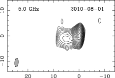
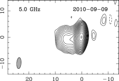
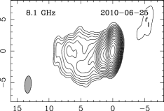
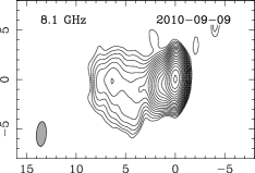
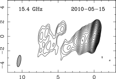
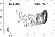
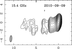
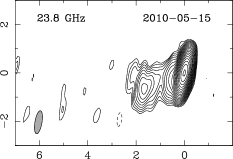
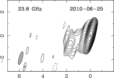
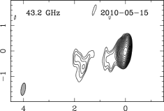
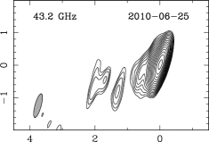
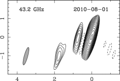
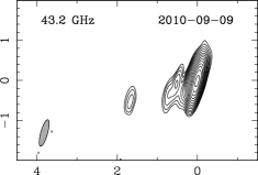
Figure 1: Naturally weighted total intensity contour maps of PKS 2233$-$148 at four epochs during 2010 at 4.6, 5.0, 8.1, 8.4, 15.4, 23.8 and 43.2 GHz, with a cell size of 0.3, 0.3, 0.2, 0.2, 0.1, 0.06, 0.03 mas per pixel, respectively. The x and y axes are given in mas of relative right ascension and relative declination, respectively. The contours are plotted at increasing powers of $\sqrt{2}$ starting from 4 rms level. The full width at half maximum (FWHM) of the restoring beam is shown as a shaded ellipse in the lower left corner. Notice that the scales in the different images are different. The image parameters are listed in Table 3.

2.3 15 GHz OVRO observations

We also used public data of PKS 2233$-$148 observations performed within the Owens Valley Radio Observatory 40-m Telescope monitoring program (Richards et al., 2011). Observations are done at 15 GHz in a 3 GHz bandwidth since 2008-10-23 to 2018-02-05 with a typical time sampling of about four days. Details of the data reduction and calibration are given in Richards et al. (2011).

2.4 Gamma-ray Fermi-LAT data

The $\gamma$-ray light curve was generated from data obtained with the LAT (Atwood et al., 2009) onboard the Fermi $\gamma$-ray space telescope between 2008-08-09 and 2016-10-17. In the analysis, we used the Fermi ScienceTools software package version v10r0p5 and Pass 8 data. In generation of the light curve, we first selected all photons between 100 MeV and 300 GeV within a $10\degr$ region of interest (ROI) around the source. In the event selection and analysis we followed the recommendations for Pass 8 data, given by the LAT team.

The photon flux over each 7-day bin was calculated using the tool gtlike with instrument response function version P8R2_SOURCE_V6. The source model was generated using the external tool make3FGLxml.py version 01 by selecting all sources within $20\degr$ of the target in the 3FGL catalogue (Acero et al., 2015), and including also the Galactic diffuse emission model version gll_iem_v06 and isotropic diffuse emission model version iso_source_v06. Based on 3FGL catalogue, the target was modeled with a log-parabola spectrum, defined as $dN/dE=N_{0}(E/E_{b})^{-(\alpha+\beta\log(E/E_{b}))}$. To account for low number of photons in each weekly bin and to reduce the number of free parameters in the fit, we froze the spectral parameters of the target and all other sources in the model to the values reported in 3FGL. For the target the 3FGL values are $\alpha=2.04$, $\beta=0.09$, and $E_{b}=581.68$. Additionally, if the source was beyond the $10\degr$ ROI or had a test statistic (TS) value (e.g., Mattox et al., 1996) less than five in 3FGL, we also froze the flux to the value reported in 3FGL. If the TS of the bin was less than four (corresponding to about 2$\sigma$) or if the number of predicted photons in that bin was less than 10, we calculated a 95% upper limit of the photon flux (Abdo et al., 2011).

3 Results

3.1 Parsec-scale jet structure

Final naturally weighted VLBA maps of the source brightness distribution at the seven frequencies at each of the four observing epochs are presented in Fig. 1. The source shows a typical parsec-scale AGN morphology of a bright compact core and one-sided jet, which propagates towards the east and is detected up to a distance of about 2 mas at 43 GHz and progressively farther, up to 8 mas at lower (4.6, 5.0 GHz) frequencies due to a steep spectrum of the jet emission (see more detailed discussion in Section 3.6). At the frequency of 8 GHz and higher the outer jet regions are transversely resolved. The lower frequency images show the faint emission beyond the core, most probably caused by the uncompensated side-lobes due to low declination of the source. The images at 8 GHz are most sensitive, with a typical noise level of about 0.16 mJy beam^-1 and a dynamic range of the order of 3000, determined as a ratio of the peak flux density to the rms noise level. The noise level was calculated as the average of rms estimates in three corner quadrants of the image, each of 1/16 of the map size. The forth quadrant, with a maximum rms was excluded being affected by the source structure. In Table 3, we summarize the VLBA map parameters.

Table 3: Summary of image parameters. Columns are as follows: (1) epoch of observations, (2) central observing frequency, (3) I peak of image, (4) rms noise level of image, (5) theoretical thermal noise estimate, (6) bottom I contour level, (7) dynamic range of image, (8) total flux density from map, (9) FWHM major axis of restoring beam, (10) FWHM minor axis of restoring beam, (11) position angle of major axis of restoring beam. The full table is available online.

Epoch	Freq.	$I_{\textrm{peak}}$	$I_{\textrm{rms}}$	Thermal noise	$I_{\textrm{base}}$	DR	$S_{\textrm{VLBA}}$	$B_{\textrm{maj}}$	$B_{\textrm{min}}$	$B_{\textrm{PA}}$
	(GHz)	(mJy bm-1)	(mJy bm-1)	(mJy bm-1)	(mJy bm-1)		(mJy)	(mas)	(mas)	(deg)
(1)	(2)	(3)	(4)	(5)	(6)	(7)	(8)	(9)	(10)	(11)
2010–05–15	4.608	335	0.19	0.11	0.76	1756	505	4.40	1.74	$-$2.0
2010–06–25	4.608	408	0.15	0.11	0.61	2676	569	4.97	1.87	$-$7.6
2010–08–01	4.608	382	0.17	0.11	0.68	2235	538	4.54	1.80	$-$3.5
2010–09–09	4.608	357	0.21	0.11	0.83	1723	510	4.50	1.79	$-$2.0
2010–05–15	5.003	350	0.18	0.15	0.71	1979	519	4.14	1.65	$-$3.3
2010–06–25	5.003	413	0.15	0.15	0.60	2737	570	4.74	1.76	$-$8.1
2010–08–01	5.003	371	0.30	0.15	1.19	1243	542	3.51	1.39	$-$2.2

Structure modeling of source brightness distribution was performed with the procedure modelfit in DIFMAP package by fitting several circular Gaussian components to the calibrated visibility data and minimizing $\chi^{2}$ in the spatial frequency plane. We used a minimum number of components (three at lower and four at higher frequencies) that after being convolved with the restoring beam, adequately reproduce the constructed source morphology. The obtained source models are listed in Table 4 and provide flux densities, positions, and sizes of the fitted components. All the positions are given with respect to the core component.

Table 4: Source models. Columns are as follows: (1) observation date, (2) name of the component, (3) flux density of the fitted Gaussian component, (4) position offset from the core component, (5) position angle of the component with respect to the core component, (6) FWHM of the fitted circular Gaussian, (7) SNR of the fitted Gaussian. The full table is available online.

Date	Comp.	Flux density	Distance	P.A.	Size	SNR
		(Jy)	(mas)	(deg)	(mas)
(1)	(2)	(3)	(4)	(5)	(6)	(7)
4.6 GHz
2010–05–15	Core	$0.304\pm 0.019$	$0.000\phantom{\,\pm\,0.000}$	…	$0.322\pm 0.014$	535
	J2	$0.127\pm 0.012$	$1.454\pm 0.036$	$113.7\pm 1.4$	$1.009\pm 0.070$	207
	J1	$0.068\pm 0.015$	$5.049\pm 0.515$	$100.5\pm 5.8$	$4.884\pm 1.030$	23
2010–06–25	Core	$0.363\pm 0.025$	$0.000\phantom{\,\pm\,0.000}$	…	$0.333\pm 0.016$	428
	J2	$0.127\pm 0.015$	$1.408\pm 0.048$	$114.2\pm 1.9$	$1.092\pm 0.094$	134
	J1	$0.068\pm 0.016$	$5.012\pm 0.557$	$103.0\pm 6.3$	$4.926\pm 1.114$	20

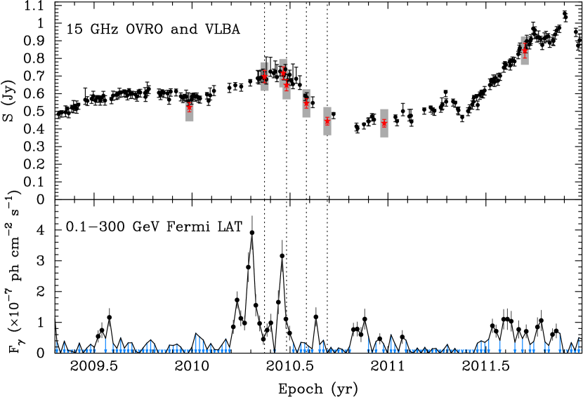
Figure 2: OVRO 15 GHz flux density evolution (top panel). Grey rectangles together with red stars indicate VLBA total flux density at 15.4 GHz, observed within our campaign S2087D and the MOJAVE program. Fermi weekly-binned $\gamma$-ray light curve at 0.1–300 GeV (bottom panel). Upper limits are given by blue arrows. Dotted vertical lines indicate the epochs of the multi-frequency VLBA observations.

3.2 Radio and $\gamma$-ray light curves

In Fig. 2, we present light curves of PKS 2233$-$148 based on the Fermi-LAT and OVRO monitoring data, complemented also by measurements of the MOJAVE program and our VLBA observations at 15 GHz. Prominent variability at high energies detected during April and June 2010 has triggered the four-epoch VLBA multi-frequency campaign. The values of the correlated VLBA total flux density are in good agreement with the single-dish OVRO flux density measurements, implying that there is almost no extended emission on kpc scales, as it was also previously concluded by Drinkwater et al. (1997). We performed a cross-correlation analysis of the light curves using the z-transformed discrete correlation function (Alexander, 1997), specifically developed for sparse, unevenly sampled light curves. The correlation between the radio and $\gamma$-ray light curves with and without upper limits is insignificant, suggesting that the $\gamma$-ray production region in the source might have a complex structure. We discuss it in more details in Section 3.9.

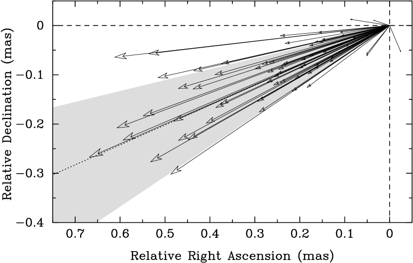
Figure 3: Core shift vectors measured in all frequency pairs. Typical error is 0.045 mas. Shaded grey area encompasses 68% of the vectors deviating less than $10\degr$ from the median jet direction shown by a dotted line.

3.3 Core shifts

The VLBI core is believed to represent the apparent jet starting region, located at the distance $r_{\text{core}}$ to the central engine, at which its optical depth reaches $\tau_{\nu}\approx 1$ at a given frequency. Thus, due to nuclear opacity, the absolute position of the radio core is frequency-dependent and varies as $r_{\text{core}}\propto\nu^{-1/k_{\text{r}}}$ (Blandford & Königl, 1979; Konigl, 1981). There is a growing observational evidence from recent multi-frequency studies of the core shift effect for $k_{\text{r}}\approx 1$ (e.g., O’Sullivan & Gabuzda, 2009; Fromm et al., 2010; Sokolovsky et al., 2011; Hada et al., 2011; Kravchenko et al., 2016; Lisakov et al., 2017). This is consistent with the Blandford & Königl (1979) model of a synchrotron self-absorbed conical jet in equipartition between energy densities of the magnetic field and the radiating particles. Departures in $k_{\text{r}}$ from unity are also possible (Plavin et al., 2018; Kutkin et al., 2014) and can be caused by pressure and density gradients in the jet or by external absorption from the surrounding medium (Lobanov, 1998; Kadler et al., 2004).

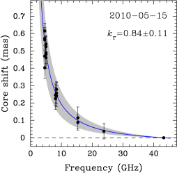
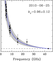
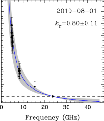
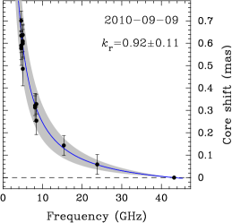
Figure 4: Frequency dependence of core shifts measured relative to the core position at 43 GHz (23 GHz for the epoch 2010-08-01) for all observational multi-frequency epochs. Solid lines represent the best power-law fits. Shaded areas show $1\sigma$ confidence regions of the fit.

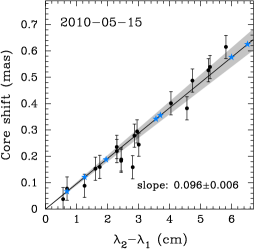
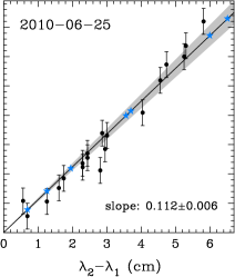
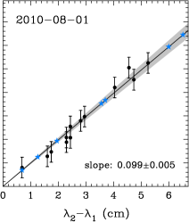
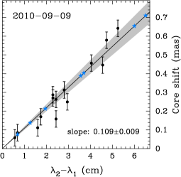
Figure 5: Core shifts as a function of difference of observing wavelengths. Solid lines represent the best linear fits. Shaded areas show $1\sigma$ confidence regions of the fit. Stars denote the expected core shifts from the true jet origin ($\lambda_{1}=0$) at wavelengths of our observations, 0.7, 1.3, 2.0, 3.6, 3.7, 6.0, 6.5 cm.

We calculated the core shift vector as $\mn@boldsymbol{\Delta r}_{\text{core},\nu_{1}\nu_{2}}=\mn@boldsymbol{\Delta r}_{12}-(\mn@boldsymbol{r}_{1}-\mn@boldsymbol{r}_{2})$, where $\mn@boldsymbol{\Delta r}_{12}$ is the displacement of the phase centers of the images at different frequencies, and $\mn@boldsymbol{r}_{1}$, $\mn@boldsymbol{r}_{2}$ are VLBI core position offsets from the phase center. To derive the image shift vector $\mn@boldsymbol{\Delta r}_{12}$, we used the fast normalized cross-correlation algorithm (Lewis, 1995) to align the images to the same position on the sky, selecting the jet regions of optically thin emission and assuming that their positions are achromatic. Every pair of images was restored with the average beam size using a pixel size of 0.03 mas.

In Fig. 3, we present a plot of 65 derived core shift vectors, where the head of each vector represents the core position at lower frequency, while all core positions at higher frequency are placed at the origin. The dotted line corresponds the median jet direction of $\text{P.A.}=112\degr$. The core shift effect occurs predominantly along the jet direction. In 68% of cases, the core shift vectors deviate less than $10\degr$ from the median jet position angle. This good alignment is achievable for a relatively straight jet, without substantial curvature in the core region. Assuming that the core shift takes place along the jet and errors are random in direction, then the standard deviation of the transverse projections of the core shift vectors onto the jet direction yields the typical error of 45 $\mu$as. Thus, in 90% of cases the derived core shifts are significantly ($>2\sigma$) different from zero. In Table 5 we list the core shift measurements: (1) epoch of observations, (2) a pair of frequencies, (3) core shift magnitude, (4) core shift direction, (5) difference of observing wavelengths.

Table 5: Core shift vectors measured for the frequency pairs $\nu_{1}$ and $\nu_{2}$. The full table is available online.

Epoch	$\nu_{1}$  $\nu_{2}$	$\Delta r_{\text{core},\nu_{1}\nu_{2}}$	P.A.	$\lambda_{2}-\lambda_{1}$
	(GHz)	(mas)	(deg)	(cm)
(1)	(2)	(3)	(4)	(5)
2010–05–15	43.2  23.8	0.038	73	0.566
2010–05–15	43.2  15.4	0.088	82	1.258
2010–05–15	43.2    8.4	0.278	106	2.865
2010–05–15	43.2    8.1	0.244	95	3.006
2010–05–15	43.2    5.0	0.539	96	5.302
2010–05–15	43.2    4.6	0.615	96	5.816
2010–05–15	23.8  15.4	0.078	138	0.692
2010–05–15	23.8    8.4	0.220	113	2.299

We have studied the frequency dependence of the core shifts (Fig. 4) by fitting a function $\Delta r_{\text{core}}=b(\nu^{-1/k_{\text{r}}}-\nu_{\text{max}}^{-1/k_{\text{r}}})$, where $b$ and $k_{\text{r}}$ are fitted parameters, and $\nu_{\text{max}}$ is fixed to the maximum frequency to which the core shifts were measured (43 GHz for the epochs 2010-05-15, 2010-06-25, and 2010-09-09; 23 GHz for the epoch 2010-08-01, at which we could not reliably measure core shift with respect to the core position at 43 GHz). The fitted $k_{\text{r}}$ values are smaller but close to one and not significantly differ from it. This can hold even during an outburst. As discussed in Plavin et al. (2018) a flare propagating down the jet disturbs only a limited portion of it, thus deviating $k_{\text{r}}$ from unity in a limited frequency range, significantly narrower compared to that of our observations. Therefore, for further analysis we use $k_{\text{r}}=1$. In this case, $r_{\text{core}}\propto\lambda$. Following the approach proposed in Voitsik et al. (2018), in Fig. 5, we plot the measured core shifts against difference in observing wavelengths (Table 5) and fit the dependence by a straight line, from which one can also estimate an offset of the apparent jet base at a given wavelength from the true jet origin by setting $\lambda_{1}=0$.

3.4 Jet shape

The core shift measurements allow us to perform a jet geometry analysis for the whole set of the fitted components including the cores. In Fig. 6, we plot the transverse jet widths $d$ as the FWHM of the fitted Gaussian components at all four multi-frequency VLBA epochs (Table 4) or the corresponding resolution limits (Kovalev et al., 2005) whichever is larger, as a function of their distance $r$ from the true jet base taking into account the core shift effect. The respective shifts $\Delta r_{\text{core}}=a(t)\lambda$ were added to the fitted core separations, where $a(t)$ is the fitted slope at a corresponding observational epoch (Fig. 5). From this analysis we excluded 16 weak components with $\text{SNR}<15$ to reduce the influence of low-SNR data points, though the whole set of 96 components yields qualitatively similar result. The BL Lac object PKS 2233$-$148 shows a conical streamline, with $d\propto r^{1.01\pm 0.04}$ at scales probed by the multi-frequency VLBA observations down to 0.1 mas. This is consistent with $k_{\text{r}}\approx 1$ derived from the core shift analysis.

The apparent jet opening angle of the source is $38\degr\pm 3\degr$, as reported by Pushkarev et al. (2017), who measured it from a stacked total intensity image at 15.4 GHz as a result of combining VLBA maps from 11 epochs distributed over a time range of about 3 yr, 2009 through 2012. The wide opening angle suggests that the jet viewing angle is rather small, of the order of a few degrees.

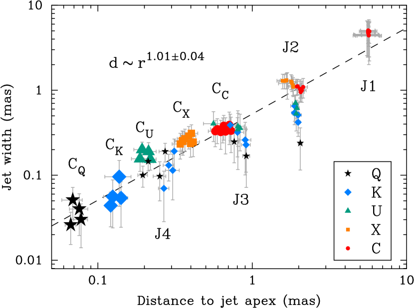
Figure 6: Jet width versus distance to the jet vertex for 78 components from structure model fits at seven frequencies of four epochs. Cores are marked by larger symbols. Dashed line is the best fit from the least square method. The jet shape at scales probed by our multi-frequency VLBA observations is conical.

3.5 Redshift constraint from the jet geometry

The optical spectrum of the source shows no prominent emission lines (Drinkwater et al., 1997) and its redshift is still unknown but the inferred conical jet shape indicates that this BL Lac object is not too close, and likely located at a redshift exceeding $\sim 0.1$. Otherwise, our VLBA observations would be sensitive enough to reveal a jet geometry transition from parabolic to conical shape, as we detect this transition in a number of nearby ($z\lesssim 0.1$) sources and explain it by a transition from magnetically to particle dominated regime in the outflows (Kovalev et al. 2018, in prep.). More distant AGNs ($z\gtrsim 0.1$) typically show close to conical jet streamlines (Pushkarev et al., 2017) since the scales probed by VLBI observations are beyond the shape transition region.

3.6 Spectral index distribution

The procedure of image registration by means of 2D cross correlation described in Section 3.3 allows to align the images at different frequencies and accurately reconstruct a distribution of spectral index $\alpha$ over the source morphology. As an example, in Fig. 7 we present spectral index map of PKS 2233$-$148 calculated between 4.6 and 23.8 GHz at the epoch 2010-09-09 of our multi-frequency VLBA observations. It shows that the core is partially opaque, with spectral index about 0.3. while the outer jet regions are optically thin, with the median value of $\alpha_{\text{jet}}=-0.95$, which is typical for many other parsec-scale AGN jets (e.g., Pushkarev & Kovalev, 2012; Hovatta et al., 2014). The spectral index error map manifests higher $\alpha$ accuracy in the innermost jet area and progressively larger uncertainties towards regions with lower brightness, where random errors dominate arising from the image noise. Systematic errors (from image alignment) dominate in the core area, especially behind it. Same result was obtained statistically for a large sample of sources in our earlier paper (see Appendix B in Hovatta et al., 2014)

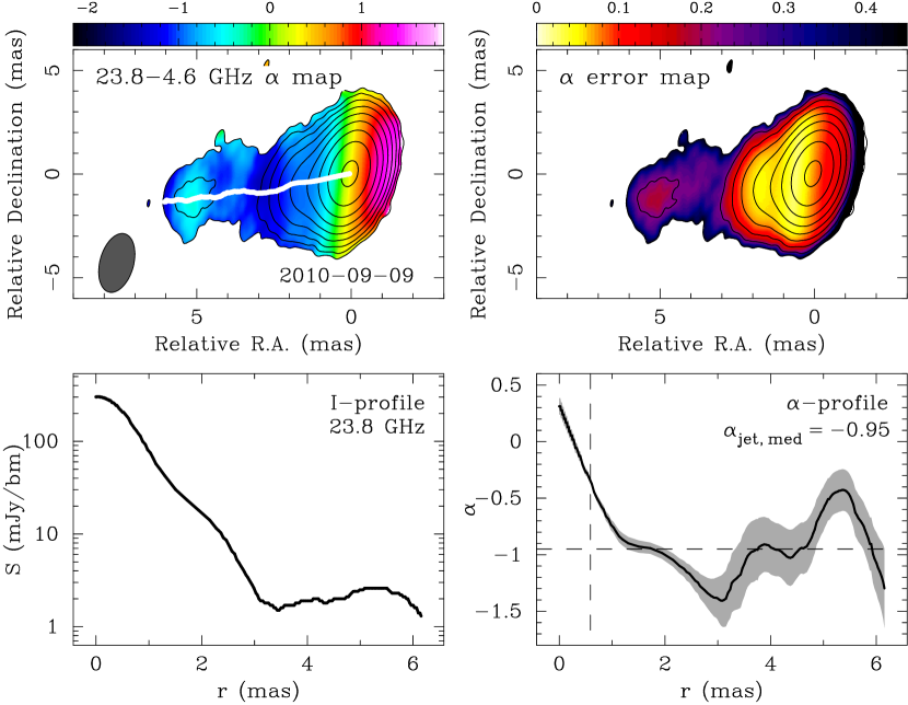
Figure 7: The distribution of the spectral index in PKS 2233$-$148 is shown in the top left panel at the epoch 2010-09-09 calculated between 4.6 and 23.8 GHz; it is shown in colour, with the 23.8 GHz total-intensity contours overlaid. The contours are plotted at increasing powers of 2, starting from 0.35% of the peak brightness of 303 mJy beam^-1. White curve denotes the total intensity ridgeline. The restoring beam is depicted, as a shaded ellipse in the lower left corner. Spectral index $1\sigma$ error map is shown in the top right panel. The bottom left and right panels show total intensity and spectral index profiles along the ridgeline, respectively. The vertical dashed line indicates the edge of the convolved VLBI core along the inner jet direction, while the horizontal dashed line represents the median jet spectral index. The grey area shows $1\sigma$ errors on the spectral index.

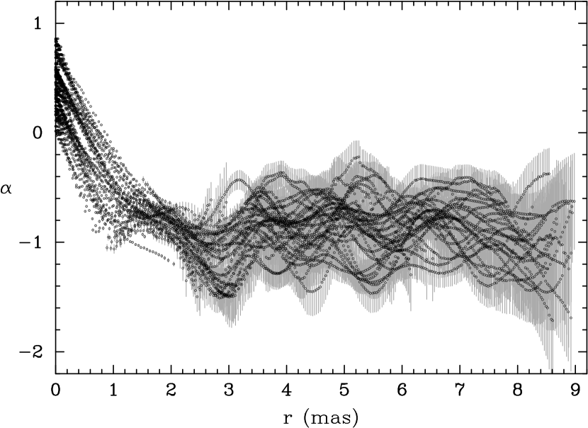
Figure 8: Spectral index evolution along the ridgeline for $\alpha$-maps restored at all frequency pairs except the 43 GHz data. The grey bars show $1\sigma$ errors.

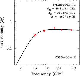
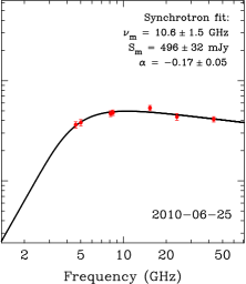
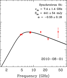
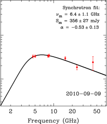
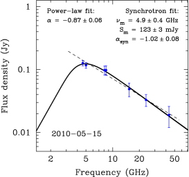
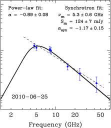
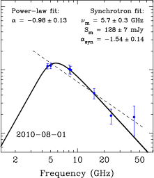
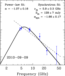
Figure 9: Spectral fits to the core (top) and jet feature J2 (bottom) data. Solid lines represent the spectra derived from the homogeneous synchrotron source model. Dashed lines show a simple power-law model. Best fit parameters of models are shown on each plot.

To analyze how spectral index changes along the jet, we reconstructed the ridgeline of the outflow in total intensity using a procedure described in Pushkarev et al. (2017). As seen from Fig. 7 (bottom right), the spectral index along the ridgeline slightly flattens in the jet knots indicating reacceleration of emitting particles, while between them it is steeper. Similar behaviour was found to be typical in AGN jets (Pushkarev & Kovalev, 2012; Hovatta et al., 2014).

Evolution of spectral index along the ridgeline for all the frequency pairs (except Q-band data) taken at all four epochs is presented in Fig. 8. Beyond the core region, the spectral index deviates around the value of about $-1$. The spectral index of optically thin synchrotron radiation parametrizes the energy spectrum of relativistic radiative particles. Assuming a power-law energy distribution $N(E)=N_{0}E^{-s}$, the power index $s=1-2\alpha$ has the mean value of $\sim 3.0$. The evolution of $\alpha_{\text{jet}}$ down the jet shows no effect of spectral aging (steepening downstream) owing to radiative losses of relativistic electrons (Kardashev, 1962), which is often seen in AGN jets on parsec-scales (Pushkarev & Kovalev, 2012). In case of PKS 2233$-$148, the absence of this effect is likely caused by the dominance of a few quasi-stationary jet features, which could be standing shocks that effectively accelerate the emitting particles.

3.7 Synchrotron spectrum fitting and magnetic field estimates

For spectral fitting of the core component (Table 4), we use the standard spectrum of a homogeneous incoherent synchrotron source of relativistic plasma with a power-law energy distribution of the form $N(E)\propto E^{-s}$ (Pacholczyk, 1970)

$$S_{\nu}\propto\nu^{5/2}\left(1-\exp\left[-\left(\frac{\nu_{1}}{\nu}\right)^{5/2-\alpha}\right]\right)\,,$$ (1)

where $\nu_{1}$ is the frequency at which the optical depth is $\tau=1$. The fitted spectra of the core are presented in Fig. 9 (top). Best fit parameters, namely the optically thin spectral index $\alpha=(1-s)/2$, the peak flux density $S_{\text{m}}$ and the corresponding self-absorption turnover frequency $\nu_{\text{m}}$ are given for every spectrum. The core component shows a spectral turnover within the frequency range of our VLBA observations.

With the fitted parameters $\nu_{\text{m}}$, $S_{\text{m}}$, and $\alpha$ of the synchrotron spectrum, we can estimate the magnetic field $B$ within the source adopting the standard synchrotron theory and assuming that the emission region is uniform and spherical. Then the commonly used expression of the component of the magnetic field perpendicular to the line of sight is (e.g. Marscher (1983); see Appendix A for more details)

$$B=10^{-5}\,b(\alpha)\,\theta_{\text{m}}^{4}\,\nu_{\text{m}}^{5}S_{\text{m}}^{\prime\,-2}\,\left(\frac{\delta}{1+z}\right)\quad[G],$$ (2)

where $\delta$ is the Doppler factor, $z$ is the redshift, $\theta_{\text{m}}$ is the diameter of the spherical component at the turnover frequency, $S_{\text{m}}^{\prime}$ is the flux density at $\nu_{\text{m}}$ extrapolated from the straight-line optically thin slope, and $b(\alpha)$ (Fig. 14) is a function of spectral index $\alpha$, optical depth $\tau_{\text{m}}$ at $\nu_{\text{m}}$, physical constants and a conversion factor, which allows one to express $\nu_{\text{m}}$ in GHz, angular size $\theta_{\text{m}}$ in mas, and $S^{\prime}_{m}$ in Jy. To derive $\theta_{\text{m}}$ we applied logarithmic interpolation between the measured component sizes at different frequencies (Table 4) and multiplied the result by a correction factor of 1.8 (Marscher, 1987) to take into account that the emission feature is assumed to have a spherical shape, while performing model fitting we measure the FWHM of the circular Gaussian components. The flux density $S_{\text{m}}^{\prime}$ can be calculated using the following relation:

$$S_{\text{m}}^{\prime}=S_{\text{m}}e^{\tau_{\text{m}}}\,,$$ (3)

where the optical depth at the turnover can be derived numerically from the equation $\exp(\tau_{\text{m}})=1+\tau_{\text{m}}(1-2\alpha/5)$ or approximated as (Türler et al., 1999)

$$\tau=\frac{3}{2}\left(\sqrt{1-\frac{16\alpha}{15}}-1\right)\,.$$ (4)

The mean value of the magnetic field inferred from Eq. (2) for the apparent core at the turnover frequency is $(0.03\pm 0.01)\delta/(1+z)$ G.

The only jet component detected at all the frequencies is J2 (see Fig. 6 and Table 4). It is located at a distance of about 2 mas from the core at 43 GHz. The spectra of this jet feature J2 in addition to a synchrotron fit was also fitted by a simple power-law (Fig. 9, bottom). The spectrum of J2 is steep, with a spectral index gradually decreasing from about $-1$ to $-1.6$, while the turnover frequency slightly increases from $4.9\pm 0.4$ GHz to $5.9\pm 0.3$ GHz.

3.8 Evolution of the turnover frequency and source kinematics

The self-absorption turnover frequency derived from the core spectra (Fig. 9, top) gradually decreases from $16.8\pm 5.3$ GHz on May 15, 2010 to $6.4\pm 1.1$ GHz on September 9, 2010 following inverse proportionality to time ($\nu_{\text{m}}\propto t^{-1}$), as predicted by a model of a conical jet with constant plasma speed (Blandford, 1990). We interpret these changes as a direct observational evidence of a flare propagation downstream. Due to synchrotron opacity in the nuclear region, the flare developing along the jet becomes detectable at progressively larger distances from the true jet origin corresponding to the VLBI core locations $r_{\text{core}}$ at longer wavelengths. After the disturbance crossed the apparent core ($\tau\approx 1$ zone) at a given frequency, its flux density starts to decrease resulting in steepening the core spectrum (Fig. 9, top) due to energy losses to synchrotron radiation or Compton scattering (Kardashev, 1962; Marscher & Gear, 1985). The core offset from the jet apex can be calculated as $r_{\text{core}}=r_{\text{flare}}=a(t)\lambda_{\text{m}}(t)$, where the parameter $a(t)$ was derived from the core shift analysis for each epoch of the multi-frequency VLBA observations (Fig. 5).

In Fig. 10, we show $r_{\text{flare}}(\lambda_{\text{m}})$ as a function of time. The slope of the weighted linear fit is $1.17\pm 0.10$ mas yr^-1. The derived proper motion of the flare propagation is significantly higher than that inferred from kinematics analysis based on tracing bright jet components. The two jet knots, J2 and J3, of the source studied within the MOJAVE program at 15 GHz are slow pattern features, with the angular speed $-71\pm 35$ $\mu$as (apparent inward motion) and $45\pm 41$ $\mu$as (Lister et al., 2016), respectively. These components are quasi-stationary and can be standing recollimation shocks observed in sources with super-magnetosonic jets (e.g., Asada & Nakamura, 2012; Cohen et al., 2014) and also obtained in numerical two-dimensional relativistic (magneto)-hydrodynamic simulations (Mizuno et al., 2015; Fromm, 2015; Fuentes et al., 2018).

Figure 10: Flare propagation down the jet. The measurements denote distances from the jet origin to the VLBI core at the frequency of maximum emission (Fig. 9, top) at the four observing VLBA epochs. Solid line represents the best linear fit. Dark and light shaded area show $1\sigma$ and $2\sigma$ confidence regions of the fit, respectively. Dot-dashed lines indicate the epoch 2010.31 of the $\gamma$-ray flare and the corresponding distance 0.12 mas of the $\gamma$-ray emission zone from the central engine. Dashed lines indicate the expected epoch range (2012) when the flare reaches the jet component J2 at 2 mas separation from the true jet base assuming constant flare propagation speed.

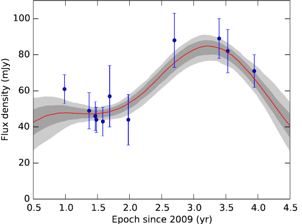
Figure 11: Flux density at 15 GHz of the jet component J2 located at 2 mas from the jet origin. The significant increase of the flux density in 2012 is likely due to the flare which originated in 2010 and reached this jet region in 2012, as expected from the assumed constant flare propagation speed. Error bars represent $1\sigma$ uncertainties of individual measurements. Smooth solid curve shows the Gaussian process fit. Dark and light filled areas correspond to 68% and 95% confidence intervals of the fit, respectively.

Since the jet geometry is found to be conical at scales probed by the VLBA observations (Sec. 3.4), we assume that the regime of constant flow speed holds at least up to 6 mas from the jet apex. Then the expected epoch for the flare to reach the quasi-stationary jet feature J2 at a distance of about 2 mas from the true jet base is $\sim$ 2012.0 (Fig. 10), at which the turnover frequency is expected to decrease down to about 1.5 GHz. This scenario is supported by a flux density evolution of the component at 15 GHz (Fig. 11). The component shows an increase of the flux density by a factor of about 2 during a period of time since $\sim 2011.5$ through $\sim 2012.5$. The epoch of the peak around 2012.0 was established by fitting the data with Gaussian process regression performed with the PyMC3 python module for Bayesian modeling, for which we used exponential quadratic covariance function. Note that moving jet components behave in a completely different manner. Typically, their brightness rapidly fades due to energy losses and adiabatic expansion (e.g., Pushkarev & Kovalev, 2012; Kravchenko et al., 2016; Lister et al., 2016).

It is therefore possible that the flare propagation rate represents the bulk flow speed. Taking into account the lower limit on redshift ($z>0.49$) derived from spectroscopy of the absorption lines formed by the intervening gas (Sbarufatti et al., 2006), the proper motion of the disturbance $\mu=1.17\pm 0.10$ mas yr^-1 corresponds to apparent speed $\beta_{\text{app}}>34\pm 2\,c$. It is much faster than a typical apparent speed $\approx 4\,c$ derived from kinematics analysis for a sample of 42 BL Lacs and also significantly higher than $\beta_{\text{app}}^{\text{max}}=21\,c$ detected in the high-redshift ($z=1.07$) BL Lac object 1514+197 (Lister et al., 2016). Similarly, analyzing multi-frequency time delays of the flares and measuring the core shifts in the blazars 3C 454.3 (Kutkin et al., 2014) and 0235+164 (Kutkin et al., 2018) it was found that this approach yields the source jet speed, which is by a factor of a few higher than the estimates based on kinematic analysis.

Now, we assume that the jet of PKS 2233$-$148 in the core region is in equipartition between the particle and magnetic field energy density ($k_{\text{r}}=1$), has a spectral index $-0.5$, and is viewed at the critical angle $\theta\simeq\Gamma^{-1}$. Then the magnetic field in Gauss at 1 pc of actual distance from the jet apex can be estimated using the following relation (Pushkarev et al., 2012)

$$B_{1}\simeq 0.04\,\Omega_{r\nu}^{3/4}\,(1+z)^{1/2}(1+\beta_{\text{app}}^{2})^{1/8}\,,$$ (5)

where $\Omega_{r\nu}$ is the core shift measure defined in Lobanov (1998) as:

$$\Omega_{r\nu}=4.85\cdot 10^{-9}\,\frac{\Delta r_{\mathrm{core,\,\nu_{1}\nu_{2}}}\,D_{L}}{(1+z)^{2}}\cdot\frac{\nu_{1}\nu_{2}}{\nu_{2}-\nu_{1}}\ \mathrm{pc\cdot GHz},$$ (6)

where $\Delta r_{\mathrm{core,\,\nu_{1}\nu_{2}}}$ is the core shift in milliarcseconds, $D_{L}$ is the luminosity distance in parsecs, and $\beta_{\text{app}}=1.58\times 10^{-8}D_{L}\mu/(1+z)$. The magnetic field strength at the apparent VLBI core at a given frequency can be calculated as $B_{\text{core}}=B_{1}r_{\text{core}}^{-1}$, where the absolute distance in parsecs of the core from the true jet base $r_{\text{core}}$ is given by Lobanov (1998)

$$r_{\text{core}}(\nu)=\frac{\Omega_{r\nu}}{\nu\sin\theta}\approx\frac{\Omega_{r\nu}(1+\beta^{2}_{\text{app}})^{1/2}}{\nu}\,,$$ (7)

where $\nu$ is the observed frequency in GHz.

In Fig. 12, we plot the derived $B_{1}$ and $B_{\text{core}}$ for the 43, 15, and 5 GHz cores as functions of redshift. Assuming $z>0.5$ the magnetic field at a distance of 1 pc from the central engine is of the order of 1 G. We note that the estimates of $B_{\text{core}}$ at 15 GHz derived from the core shift analysis are comparable (lower by a factor of a few) to those inferred from the synchrotron spectrum fits (Sec. 3.7), if a source Doppler factor is moderate ($\delta\lesssim 5$), as often observed in BL Lacertae objects (Hovatta et al., 2009; Liodakis et al., 2017).

3.9 Location of the $\gamma$-ray emission region and the source of seed photons

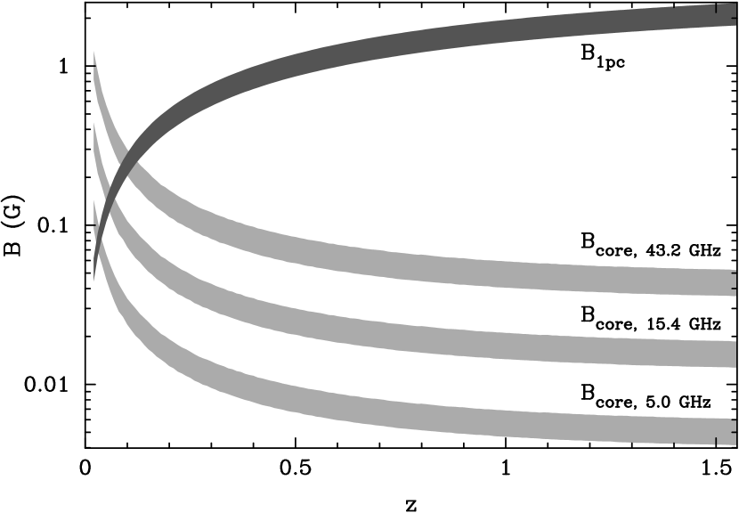
Figure 12: Magnetic field constraints obtained from the core shift measurements and the flare propagation speed. Dark grey area show estimates of the magnetic field at 1 pc distance from the jet origin, while light grey stripes represent the magnetic field at the core at 43,2, 15,4 and 5.0 GHz.

To estimate the location of the $\gamma$-ray emission zone in PKS 2233$-$148 we extrapolated the $r_{\text{flare}}$ dependence (Fig. 10) back to the epoch of the $\gamma$-ray flare, 2010.31 (Fig. 2). This yields an angular separation of $0.12\pm 0.03$ mas from the true jet base, which corresponds to the VLBI core position at 24 GHz (Fig. 6). On a linear scale, this separation is $>0.7\pm 0.2$ pc in projection, which exceeds a de-projected separation of $8\pm 2$ pc if we assume a jet viewing angle of $5\degr$. Considering the second peak of the $\gamma$-ray data at epoch 2010.46 (June 17, 2010), we inferred distance of about 0.3 mas from the jet apex. This distance corresponds to the innermost jet feature J4 detected at 24 and 43 GHz setting an absolute distance of about 20 pc for another possible location of the $\gamma$-ray emission site. These assessments favour a scenario for the $\gamma$-ray production zone to be located at large distances from a central energy generator (beyond the broad-line region or torus) and likely associated with one or more standing shocks in a relativistic outflow of PKS 2233$-$148, as hinted by a complex structure of the major high-energy flares in the source. Similar conclusion regarding remotness of the $\gamma$-ray emission region in blazars on scales of parsecs from the central black hole was also made from other arguments in a number of recent single-source studies of 1510$-$089 (Marscher et al., 2010), OJ 287 (Agudo et al., 2011), 3C 345 (Schinzel et al., 2012), CTA 102 (Casadio et al., 2015), 1502+106 (Karamanavis et al., 2016), BL Lacertae (Wehrle et al., 2016), and also statistical results from F-GAMMA project (Fuhrmann et al., 2016). At the same time, the arguments based on short-scale variability and breaks in GeV spectra discussed in Introduction indicate that the high-energy production site is in the immediate vicinity of the black hole.

Another noticeable feature of the pc-scale morphology of the source is a presence of a sheath around the jet, the indications of which are seen at 8 and 15 GHz maps (Fig. 1) that provide a combination of a high angular resolution and sensitivity. To better visualize the sheath emission we convolved the 8.1 GHz image at the epoch 2010-05-15 with a circular beam setting its FWHM to that of the minor axis of the original map (Fig. 13). The fact that this sheath is slower than a central spine might mean that it acts as a source of additional seed photons for the $\gamma$-ray radiation (e.g., Marscher et al., 2010; Aleksić et al., 2014). Thus, the high-energy emission of the source can be formed through (i) synchrotron self-Compton mechanism acting in its relativistic outflow and upscattering of low-energy synchrotron seed photons and (ii) external Compton scattering due to a photon field in the sheath.

While detailed modeling of the spectral energy distribution (SED) is beyond the scope of this paper, based on the publicly available non-simultaneous data in the SSDC SED builder tool, it seems that when the source is in a high state in $\gamma$-rays, the luminosity of the inverse Compton peak is higher than that of the synchrotron peak, indicating that an additional external photon field is indeed needed. However, this should be verified with simultaneous data in all bands, taken at both low and high activity states of the source.

We can also speculate that if instead of the epoch of the $\gamma$-ray peak we consider the epoch when the flare starts rising (a few weeks before the peak), then the $\gamma$-ray emission site could be in the immediate vicinity of the central machine. But this scenario is vulnerable as a plasma cloud moving fast down the jet leaves the seed photon area rapidly, while the flare is still reaching its maximum.

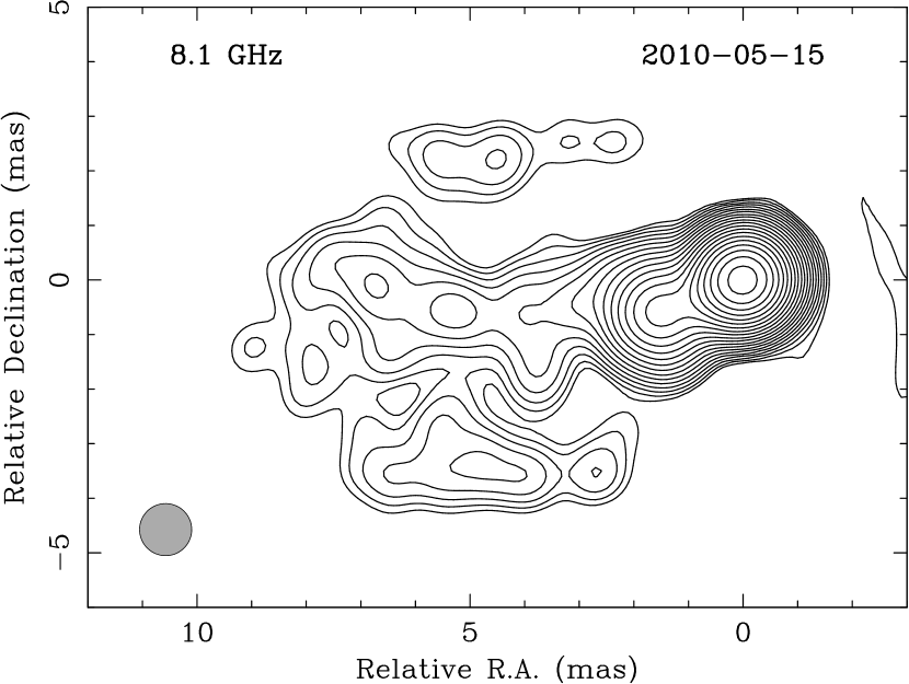
Figure 13: Total intensity map of PKS 2233$-$148 at 8.1 GHz at the epoch 2010-05-15 from Fig. 1 but convolved with a circular beam of a size of the minor axis of the original image. Emission at the jet edges indicate a presence of a distinct boundary layer.

4 Summary

We performed a radio and $\gamma$-ray joint study of the BL Lacertae object PKS 2233$-$148, using multiwavelength data in the period of 2009–2012. The 4.6–43.2 GHz VLBA observations reveal the core dominated, one-sided and relatively straight jet morphology of the source extending up to 8 mas in a position angle $112\degr$. Analyzing jet widths derived from the structure model fits we have established that the outflow has a conical shape. This sets a lower limit of about 0.1 on the source unknown redshift.

We have measured the frequency-dependent shift vectors of the apparent core position using a method based on results from (i) structure model fitting and (ii) image alignment achieved by implementing a two-dimensional cross-correlation technique on the optically thin jet regions. The magnitude of the core shifts ranges from 0.04 to 0.7 mas, with a typical uncertainty of 45 $\mu$as. The directions of the shift vectors are predominantly aligned with the median jet position angle, deviating from it by $\lesssim 10\degr$ in 68% of cases. The derived core shifts show a frequency dependence $\propto\nu^{-1/k_{\text{r}}}$, with $k_{r}\approx 1$ indicating that nuclear opacity is dominated by synchrotron self-absorption, and physical conditions in the jet on scales probed by the VLBA observations are close to equipartition. We did not find an evidence for significant changes in $k_{\text{r}}$ between the observing epochs covering a time scale of four months, during which a flare was developing down the jet. It suggests that the transverse size of the disturbance area is significantly smaller than the jet part constrained by the magnitude of the core shift effect within a frequency range 5–43 GHz. The VLBI core position $r_{\text{core}}$, as a function of wavelength follows an $r_{\text{mas}}^{\text{core}}\approx 0.1\lambda_{\text{cm}}$ dependence. The magnetic field at a distance of 1 pc from the jet apex derived from the core shift measurements is about 1 G.

We present a method of independent assessment of jet kinematics based on core shift measurements and evolution of synchrotron spectrum of the VLBI core. The turnover frequency of the core spectrum linearly shifts towards lower frequencies with time, as the flare originated in April 2010 in $\gamma$-rays propagates down the jet. The speed of this propagation is about 1.2 mas yr^-1 and likely represents the bulk flow speed. It is much higher comparing to results from traditional kinematics based on tracking bright jet features, 0.045 mas yr^-1 (Lister et al., 2016).

We have found indications that the $\gamma$-ray production zone in the source is located at large distances, 10–20 pc, from a central engine, and can be associated with the stationary radio-emitting jet features observed with VLBI. This favours synchrotron self-Compton scattering as a dominant high-energy radiation mechanism in the relativistic jet of the source. Direct observational evidence for a boundary layer around the jet suggests that the sheath might be an additional source of seed photons for external Compton scattering acting in the source.

Appendix A Magnetic field from synchrotron self-absorption

Interpretation of a radio spectrum with the low-frequency turnover caused by synchrotron self-absorption, and determination of physical parameters within this assumption date back to the 1960s (see, for example, one of the pioneering works Slish, 1963). In particular, magnetic field associated with a source of synchrotron emission can be inferred. However, the approximate values of the numerical coefficient in the formula that are a function of a spectral index $\alpha$ ($S_{\nu}\propto\nu^{\alpha}$) of the optically thin part of a synchrotron spectrum are tabulated for a limited number of $\alpha$ values ranging from $-0.25$ to $-$1.0 (Marscher, 1983). The relation for this coefficient was previously discussed by Gould (1979). In this Appendix, we derive a formula for this coefficient that can be computed precisely.

Following Pacholczyk (1970), intensity of emission in a case of synchrotron self-absorption is

$$S_{\nu}=F\left(\nu_{1}\right)J\left(\frac{\nu}{\nu_{1}},s\right)\,,$$ (8)

where $s=1-2\alpha$ is the power-law index of energy distribution $N\left(E\right)=N_{0}E^{-s}$ of emitting electrons, and

$$J\left(\frac{\nu}{\nu_{1}},s\right)=\left(\frac{\nu}{\nu_{1}}\right)^{5/2}\left\{1-\exp\left[-\left(\frac{\nu}{\nu_{1}}\right)^{-\left(s+4\right)/2}\right]\right\}\,,$$ (9)

where $\nu_{1}$ is the frequency at which the optical depth $\tau=1$. Source function $F\left(\nu_{1}\right)$ for a spherical, uniform emitting region with observed angular size $\theta=2R(1+z)^{2}/D$ at the luminosity distance $D$ is

$$F\left(\nu_{1}\right)=\frac{\left(\pi\theta^{2}R/3\right)\varepsilon_{\nu_{1}}\left[\delta/\left(1+z\right)\right]^{2-\alpha}}{2\kappa_{\nu_{1}}R\left[\delta/\left(1+z\right)\right]^{\left(3-2\alpha\right)/2}}=\\ =\frac{\pi}{6}\theta^{2}\frac{\varepsilon_{\nu_{1}}}{\kappa_{\nu_{1}}}\left(\frac{\delta}{1+z}\right)^{1/2},$$ (10)

where

$$\varepsilon_{\nu_{1}}=c_{5}\left(s\right)N_{0}B_{\bot}^{\left(s+1\right)/2}\left(\frac{\nu_{1}}{2c_{1}}\right)^{\left(1-s\right)/2}$$ (11)

and

$$\kappa_{\nu_{1}}=c_{6}\left(s\right)N_{0}B_{\bot}^{\left(s+2\right)/2}\left(\frac{\nu_{1}}{2c_{1}}\right)^{-\left(s+4\right)/2}$$ (12)

are the emission and absorption coefficients, respectively, $B_{\bot}$ is the component of the magnetic field perpendicular to the line of sight. Constants and functions are:

$$c_{1}=\frac{3e}{4\pi m^{3}c^{5}}\,,\qquad c_{3}=\frac{\sqrt{3}e^{3}}{4\pi mc^{2}}\,,$$ (13)

$$c_{5}=\frac{1}{4}c_{3}\frac{s+7/3}{s+1}\,\,\Gamma\left(\frac{3s-1}{12}\right)\Gamma\left(\frac{3s+7}{12}\right)\,,$$ (14)

$$c_{6}=\frac{1}{32}\left(\frac{c}{c_{1}}\right)^{2}c_{3}\left(s+\frac{10}{3}\right)\Gamma\left(\frac{3s+2}{12}\right)\Gamma\left(\frac{3s+10}{12}\right),$$ (15)

where $e$ and $m$ are the charge and mass of electron, respectively, $c$ is the speed of light in vacuum, and $\Gamma$ is the Euler gamma function.

Substituting Eqs. (9)-(15) into (8) we obtain

$$S_{\nu}=\frac{\pi}{6}\,\frac{c_{5}\left(s\right)}{c_{6}\left(s\right)}\left(2c_{1}\right)^{-5/2}\theta^{2}B_{\bot}^{-1/2}\nu^{5/2}\left(\frac{\delta}{1+z}\right)^{1/2}\left[1-\text{e}^{-\tau_{\nu}}\right],$$ (16)

where $\tau_{\nu}=\left(\nu/\nu_{1}\right)^{-\left(s+4\right)/2}$. Then the flux density at the turnover frequency $\nu_{\text{m}}$ extrapolated from the straight-line slope of the optically thin part of synchrotron spectrum is

$$S_{\text{m}}^{\prime}=\left.S_{\nu}\right|_{\nu=\nu_{m}}\text{e}^{\tau_{\text{m}}}=\\ =\left[\frac{\pi}{6}\frac{c_{5}\left(s\right)}{c_{6}\left(s\right)}\left(2c_{1}\right)^{-5/2}(e^{\tau_{\text{m}}}-1)\right]\theta^{2}B_{\bot}^{-1/2}\nu_{\text{m}}^{5/2}\left(\frac{\delta}{1+z}\right)^{1/2}\,.$$ (17)

The optical depth $\tau_{\text{m}}$ at $\nu_{\text{m}}$ is found from equation

$$\text{e}^{\tau_{\text{m}}}=1+\left(1-\frac{2\alpha}{5}\right)\tau_{\text{m}}\,.$$ (18)

By developing the exponential in Eq. (18) to the third order, Türler et al. (1999) obtained the approximate solution

$$\tau_{\text{m}}=\frac{3}{2}\left(\sqrt{1-\frac{16\alpha}{15}}-1\right)\,,$$ (19)

which is accurate enough, deviating less than 5% from the exact numerical solution for $\alpha\gtrsim-1.55$ (Fig. 14).

Solving Eq. (17) for the normal component of magnetic field, we have

$$B_{\bot}=10^{-5}\,b\left(s\right)\,\theta^{4}\,S_{\text{m}}^{\prime\,-2}\,\nu_{\text{m}}^{5}\left(\frac{\delta}{1+z}\right)\,,$$ (20)

where the source size $\theta$ is in milliarcseconds, flux density in Jy, the turnover frequency $\nu_{m}$ in GHz, and the magnetic field in G.

$$b\left(s\right)=5.5\cdot 10^{62}\left[\frac{\pi}{6}\frac{c_{5}\left(s\right)}{c_{6}\left(s\right)}(e^{\tau_{\text{m}}}-1)\right]^{2}\left(2c_{1}\right)^{-5}\,.$$ (21)

In Fig. 14, we plot the coefficient $b$ as a function of $\alpha=(1-s)/2$. The departure of the approximate solutions from exact ones exceeds 5% for $\alpha\lesssim-0.82$.

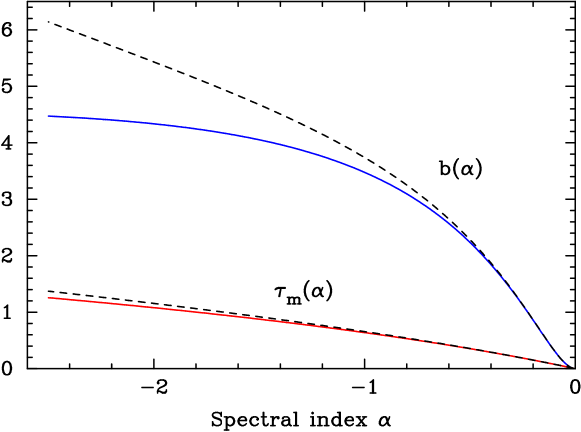
Figure 14: Coefficient $b(\alpha)$ and optical depth $\tau_{\text{m}}(\alpha)$ as a function of spectral index $\alpha$. Dashed lines represent approximate solutions derived by using Eq. 19.

Table 6: Amplitude scale corrections for the S2087D VLBA experiment.

Antenna	Band	Epoch	IF	Correction
(1)	(2)	(3)	(4)	(5)
BR	K	1	1–2	0.88
BR	K	1	3–4	0.85
BR	K	2,3,4	1–4	0.80
FD	U	1	1–4	1.09
FD	Q	1	1–4	1.15
KP	C	2,4	1–2	1.08
KP	X	1	1–2	0.90
KP	X	2,3,4	1–2	0.93
KP	K	All	1–4	1.10
LA	C	All	1–2	0.93
LA	K	All	1–4	0.90
OV	X	1	1–2	1.21
OV	X	3,4	1–2	1.17
SC	U	1	1–4	0.88
SC	Q	2	2,4	0.80

Column designation: (1) antenna name; (2) radio band name; (3) observation epoch (epochs are labeled as follows: 1 for 2010-05-15, 2 for 2010-06-25, 3 for 2010-08-01, 4 for 2010-09-09); (4) number of the frequency channel (IF); (5) amplitude scale correction coefficient.

Table 7: Summary of image parameters. Columns are as follows: (1) epoch of observations, (2) central observing frequency, (3) I peak of image, (4) rms noise level of image, (5) thermal noise estimate, (6) bottom I contour level, (7) dynamic range of image, (8) total flux density from map, (9) FWHM major axis of restoring beam, (10) FWHM minor axis of restoring beam, (11) position angle of major axis of restoring beam.

Epoch	Freq.	$I_{\textrm{peak}}$	$I_{\textrm{rms}}$	Thermal noise	$I_{\textrm{base}}$	DR	$S_{\textrm{VLBA}}$	$B_{\textrm{maj}}$	$B_{\textrm{min}}$	$B_{\textrm{PA}}$
	(GHz)	(mJy bm-1)	(mJy bm-1)	(mJy bm-1)	(mJy bm-1)		(mJy)	(mas)	(mas)	(deg)
(1)	(2)	(3)	(4)	(5)	(6)	(7)	(8)	(9)	(10)	(11)
2010-05-15	4.608	335	0.19	0.11	0.76	1756	505	4.40	1.74	$-$2.0
2010-06-25	4.608	408	0.15	0.11	0.61	2676	569	4.97	1.87	$-$7.6
2010-08-01	4.608	382	0.17	0.11	0.68	2235	538	4.54	1.80	$-$3.5
2010-09-09	4.608	357	0.21	0.11	0.83	1723	510	4.50	1.79	$-$2.0
2010-05-15	5.003	350	0.18	0.15	0.71	1979	519	4.14	1.65	$-$3.3
2010-06-25	5.003	413	0.15	0.15	0.60	2737	570	4.74	1.76	$-$8.1
2010-08-01	5.003	371	0.30	0.15	1.19	1243	542	3.51	1.39	$-$2.2
2010-09-09	5.003	359	0.17	0.15	0.68	2115	514	4.21	1.67	$-$2.2
2010-05-15	8.108	438	0.15	0.16	0.59	2963	588	2.35	0.95	$-$0.7
2010-06-25	8.108	470	0.18	0.16	0.70	2677	615	2.71	1.03	$-$5.9
2010-08-01	8.108	417	0.17	0.16	0.69	2410	566	2.46	0.97	$-$1.7
2010-09-09	8.108	335	0.15	0.16	0.61	2203	478	2.49	0.99	$-$1.8
2010-05-15	8.429	445	0.16	0.16	0.64	2778	595	2.31	0.92	$-$2.2
2010-06-25	8.429	477	0.14	0.16	0.56	3429	624	2.68	0.99	$-$7.5
2010-08-01	8.429	425	0.16	0.16	0.63	2707	569	2.44	0.95	$-$3.1
2010-09-09	8.429	345	0.14	0.16	0.58	2396	487	2.45	0.96	$-$3.1
2010-05-15	15.365	557	0.20	0.18	0.68	2853	697	1.58	0.49	$-$11.9
2010-06-25	15.365	517	0.19	0.18	0.66	2735	648	1.57	0.51	$-$10.2
2010-08-01	15.365	406	0.19	0.18	0.65	2179	545	1.37	0.48	$-$6.6
2010-09-09	15.365	296	0.19	0.18	0.68	1523	426	1.38	0.48	$-$6.4
2010-05-15	23.804	557	0.26	0.21	1.02	2181	685	0.96	0.29	$-$12.3
2010-06-25	23.804	496	0.33	0.21	1.30	1521	616	1.12	0.29	$-$15.4
2010-08-01	23.804	320	0.27	0.21	1.10	1167	449	0.95	0.27	$-$12.6
2010-09-09	23.804	250	0.26	0.21	1.06	945	350	1.19	0.31	$-$15.2
2010-05-15	43.217	511	0.40	0.32	1.41	1271	631	0.49	0.17	$-$8.5
2010-06-25	43.217	450	0.44	0.32	1.55	1013	583	0.75	0.19	$-$16.9
2010-08-01	43.217	442	0.92	0.45	3.23	479	585	0.97	0.19	$-$16.3
2010-09-09	43.217	346	0.96	0.45	3.36	361	439	0.68	0.17	$-$14.3

Table 8: Source models. Columns are as follows: (1) observation date, (2) name of the component, (3) flux density of the fitted Gaussian component, (4) position offset from the core component, (5) position angle of the component with respect to the core component, (6) FWHM major axis of the fitted Gaussian, (7) SNR of the fitted Gaussian.

Date	Comp.	Flux density	Distance	P.A.	Size	SNR
		(Jy)	(mas)	(deg)	(mas)
(1)	(2)	(3)	(4)	(5)	(6)	(7)
4.6 GHz
2010-05-15	Core	$0.304\pm 0.019$	$0.000\phantom{\,\pm\,0.000}$	…	$0.322\pm 0.014$	535
	J2	$0.127\pm 0.012$	$1.454\pm 0.036$	$113.7\pm 1.4$	$1.009\pm 0.070$	207
	J1	$0.068\pm 0.015$	$5.049\pm 0.515$	$100.5\pm 5.8$	$4.884\pm 1.030$	23
2010-06-25	Core	$0.363\pm 0.025$	$0.000\phantom{\,\pm\,0.000}$	…	$0.333\pm 0.016$	428
	J2	$0.127\pm 0.015$	$1.408\pm 0.048$	$114.2\pm 1.9$	$1.092\pm 0.094$	134
	J1	$0.068\pm 0.016$	$5.012\pm 0.557$	$103.0\pm 6.3$	$4.926\pm 1.114$	20
2010-08-01	Core	$0.350\pm 0.020$	$0.000\phantom{\,\pm\,0.000}$	…	$0.356\pm 0.014$	618
	J2	$0.115\pm 0.011$	$1.394\pm 0.040$	$112.0\pm 1.6$	$1.039\pm 0.078$	180
	J1	$0.065\pm 0.013$	$4.997\pm 0.461$	$102.1\pm 5.3$	$4.706\pm 0.922$	27
2010-09-09	Core	$0.327\pm 0.026$	$0.000\phantom{\,\pm\,0.000}$	…	$0.391\pm 0.022$	315
	J2	$0.109\pm 0.014$	$1.333\pm 0.051$	$115.2\pm 2.1$	$1.026\pm 0.100$	104
	J1	$0.066\pm 0.014$	$4.939\pm 0.479$	$101.6\pm 5.5$	$4.722\pm 0.958$	25
5.0 GHz
2010-05-15	Core	$0.329\pm 0.020$	$0.000\phantom{\,\pm\,0.000}$	…	$0.329\pm 0.014$	547
	J2	$0.117\pm 0.012$	$1.485\pm 0.038$	$113.4\pm 1.4$	$0.951\pm 0.074$	166
	J1	$0.067\pm 0.016$	$5.057\pm 0.572$	$101.9\pm 6.5$	$4.918\pm 1.144$	19
2010-06-25	Core	$0.382\pm 0.027$	$0.000\phantom{\,\pm\,0.000}$	…	$0.326\pm 0.016$	387
	J2	$0.114\pm 0.014$	$1.425\pm 0.046$	$112.4\pm 1.8$	$0.997\pm 0.090$	125
	J1	$0.067\pm 0.014$	$4.967\pm 0.508$	$102.7\pm 5.8$	$5.053\pm 1.016$	26
2010-08-01	Core	$0.360\pm 0.021$	$0.000\phantom{\,\pm\,0.000}$	…	$0.349\pm 0.014$	560
	J2	$0.117\pm 0.012$	$1.376\pm 0.043$	$113.3\pm 1.7$	$1.113\pm 0.084$	173
	J1	$0.059\pm 0.014$	$5.088\pm 0.499$	$103.1\pm 5.6$	$4.484\pm 0.998$	21
2010-09-09	Core	$0.331\pm 0.021$	$0.000\phantom{\,\pm\,0.000}$	…	$0.382\pm 0.018$	474
	J2	$0.115\pm 0.013$	$1.295\pm 0.047$	$115.3\pm 2.0$	$1.107\pm 0.092$	145
	J1	$0.060\pm 0.013$	$5.033\pm 0.452$	$101.2\pm 5.1$	$4.413\pm 0.904$	25
8.1 GHz
2010-05-15	Core	$0.449\pm 0.032$	$0.000\phantom{\,\pm\,0.000}$	…	$0.250\pm 0.012$	376
	J2	$0.098\pm 0.016$	$1.491\pm 0.073$	$112.4\pm 2.8$	$1.096\pm 0.146$	57
	J1	$0.044\pm 0.019$	$5.387\pm 0.931$	$101.0\pm 9.8$	$4.357\pm 1.862$	6
2010-06-25	Core	$0.469\pm 0.031$	$0.000\phantom{\,\pm\,0.000}$	…	$0.246\pm 0.012$	438
	J2	$0.106\pm 0.015$	$1.374\pm 0.076$	$113.0\pm 3.2$	$1.269\pm 0.152$	72
	J1	$0.043\pm 0.017$	$5.323\pm 0.871$	$102.0\pm 9.3$	$4.383\pm 1.742$	7
2010-08-01	Core	$0.420\pm 0.030$	$0.000\phantom{\,\pm\,0.000}$	…	$0.269\pm 0.014$	393
	J2	$0.103\pm 0.016$	$1.303\pm 0.087$	$113.2\pm 3.8$	$1.313\pm 0.174$	58
	J1	$0.045\pm 0.018$	$5.244\pm 0.893$	$101.3\pm 9.7$	$4.421\pm 1.786$	7
2010-09-09	Core	$0.335\pm 0.023$	$0.000\phantom{\,\pm\,0.000}$	…	$0.311\pm 0.016$	397
	J2	$0.101\pm 0.014$	$1.216\pm 0.076$	$114.8\pm 3.6$	$1.284\pm 0.152$	72
	J1	$0.043\pm 0.017$	$5.199\pm 0.916$	$101.5\pm 10.0$	$4.500\pm 1.832$	7
8.4 GHz
2010-05-15	Core	$0.455\pm 0.034$	$0.000\phantom{\,\pm\,0.000}$	…	$0.233\pm 0.012$	359
	J2	$0.098\pm 0.017$	$1.495\pm 0.082$	$112.7\pm 3.1$	$1.137\pm 0.164$	50
	J1	$0.044\pm 0.021$	$5.352\pm 1.036$	$103.6\pm 11.0$	$4.382\pm 2.072$	5
2010-06-25	Core	$0.480\pm 0.030$	$0.000\phantom{\,\pm\,0.000}$	…	$0.236\pm 0.010$	508
	J2	$0.099\pm 0.015$	$1.410\pm 0.074$	$112.8\pm 3.0$	$1.217\pm 0.148$	69
	J1	$0.044\pm 0.017$	$5.318\pm 0.830$	$103.1\pm 8.9$	$4.350\pm 1.660$	8
2010-08-01	Core	$0.429\pm 0.030$	$0.000\phantom{\,\pm\,0.000}$	…	$0.255\pm 0.012$	411
	J2	$0.100\pm 0.015$	$1.313\pm 0.085$	$112.6\pm 3.7$	$1.304\pm 0.170$	59
	J1	$0.043\pm 0.017$	$5.261\pm 0.853$	$102.6\pm 9.2$	$4.453\pm 1.706$	8
2010-09-09	Core	$0.343\pm 0.026$	$0.000\phantom{\,\pm\,0.000}$	…	$0.289\pm 0.016$	336
	J2	$0.102\pm 0.015$	$1.187\pm 0.080$	$114.3\pm 3.9$	$1.291\pm 0.160$	66
	J1	$0.045\pm 0.018$	$5.144\pm 0.878$	$102.7\pm 9.7$	$4.551\pm 1.756$	8

Table 9: continued

Date	Comp.	Flux density	Distance	P.A.	Size	SNR
		(Jy)	(mas)	(deg)	(mas)
(1)	(2)	(3)	(4)	(5)	(6)	(7)
15.4 GHz
2009-12-26	Core	$0.383\pm 0.021$	$0.000\phantom{\,\pm\,0.000}$	…	$0.120\pm 0.004$	680
	J3	$0.051\pm 0.008$	$0.421\pm 0.029$	$114.6\pm 3.9$	$0.447\pm 0.058$	59
	J2	$0.061\pm 0.008$	$1.715\pm 0.021$	$111.0\pm 0.7$	$0.430\pm 0.042$	102
	J1	$0.030\pm 0.018$	$5.341\pm 1.434$	$101.5\pm 15.0$	$4.726\pm 2.868$	4
2010-05-15	Core	$0.584\pm 0.039$	$0.000\phantom{\,\pm\,0.000}$	…	$0.156\pm 0.008$	448
	J3	$0.037\pm 0.010$	$0.619\pm 0.035$	$115.0\pm 3.2$	$0.334\pm 0.070$	24
	J2	$0.049\pm 0.010$	$1.740\pm 0.043$	$111.2\pm 1.4$	$0.530\pm 0.086$	40
	J1	$0.031\pm 0.024$	$5.299\pm 1.679$	$98.0\pm 17.6$	$4.379\pm 3.358$	2
2010-06-19	Core	$0.577\pm 0.027$	$0.000\phantom{\,\pm\,0.000}$	…	$0.130\pm 0.006$	922
	J3	$0.059\pm 0.009$	$0.520\pm 0.034$	$119.2\pm 3.7$	$0.358\pm 0.068$	86
	J2	$0.046\pm 0.007$	$1.719\pm 0.037$	$111.3\pm 1.2$	$0.625\pm 0.074$	79
	J1	$0.034\pm 0.017$	$5.218\pm 1.150$	$100.3\pm 12.4$	$4.714\pm 2.300$	5
2010-06-25	Core	$0.534\pm 0.029$	$0.000\phantom{\,\pm\,0.000}$	…	$0.154\pm 0.006$	650
	J3	$0.045\pm 0.009$	$0.589\pm 0.028$	$118.4\pm 2.7$	$0.377\pm 0.056$	46
	J2	$0.044\pm 0.007$	$1.727\pm 0.042$	$110.8\pm 1.4$	$0.615\pm 0.084$	55
	J1	$0.029\pm 0.021$	$5.411\pm 1.624$	$102.0\pm 16.7$	$4.606\pm 3.248$	3
2010-08-01	Core	$0.439\pm 0.031$	$0.000\phantom{\,\pm\,0.000}$	…	$0.200\pm 0.010$	380
	J3	$0.041\pm 0.010$	$0.641\pm 0.032$	$118.4\pm 2.9$	$0.358\pm 0.064$	32
	J2	$0.043\pm 0.008$	$1.716\pm 0.057$	$112.9\pm 1.9$	$0.705\pm 0.114$	40
	J1	$0.027\pm 0.020$	$5.335\pm 1.530$	$100.1\pm 16.0$	$4.187\pm 3.060$	3
2010-09-09	Core	$0.298\pm 0.025$	$0.000\phantom{\,\pm\,0.000}$	…	$0.190\pm 0.012$	274
	J3	$0.055\pm 0.012$	$0.348\pm 0.035$	$100.4\pm 5.6$	$0.404\pm 0.068$	37
	J2	$0.057\pm 0.017$	$1.474\pm 0.164$	$110.6\pm 6.3$	$1.198\pm 0.328$	14
	J1	$0.022\pm 0.017$	$5.771\pm 1.463$	$99.1\pm 14.2$	$3.910\pm 2.926$	2
2010-12-24	Core	$0.306\pm 0.019$	$0.000\phantom{\,\pm\,0.000}$	…	$0.000\pm 0.010$	526
	J3	$0.060\pm 0.009$	$0.442\pm 0.031$	$98.9\pm 4.0$	$0.171\pm 0.062$	88
	J2	$0.046\pm 0.009$	$1.411\pm 0.077$	$110.5\pm 3.1$	$0.790\pm 0.154$	36
	J1	$0.023\pm 0.022$	$4.943\pm 2.275$	$95.5\pm 24.7$	$4.094\pm 4.550$	2
2011-09-12	Core	$0.644\pm 0.039$	$0.000\phantom{\,\pm\,0.000}$	…	$0.000\pm 0.008$	559
	J3	$0.071\pm 0.014$	$0.269\pm 0.073$	$103.3\pm 15.2$	$0.756\pm 0.146$	32
	J2	$0.088\pm 0.015$	$1.611\pm 0.044$	$110.7\pm 1.6$	$0.494\pm 0.088$	54
	J1	$0.029\pm 0.032$	$5.275\pm 2.814$	$101.1\pm 28.1$	$4.401\pm 5.628$	1
2012-05-24	Core	$1.029\pm 0.034$	$0.000\phantom{\,\pm\,0.000}$	…	$0.090\pm 0.002$	1785
	J3	$0.053\pm 0.008$	$0.506\pm 0.032$	$94.3\pm 3.6$	$0.286\pm 0.064$	79
	J2	$0.089\pm 0.011$	$1.612\pm 0.031$	$113.0\pm 1.1$	$0.609\pm 0.062$	100
	J1	$0.027\pm 0.016$	$5.417\pm 1.109$	$101.0\pm 11.6$	$3.927\pm 2.218$	4
2012-07-12	Core	$0.716\pm 0.028$	$0.000\phantom{\,\pm\,0.000}$	…	$0.140\pm 0.004$	1273
	J3	$0.066\pm 0.009$	$0.538\pm 0.026$	$98.9\pm 2.8$	$0.328\pm 0.052$	94
	J2	$0.082\pm 0.012$	$1.561\pm 0.034$	$114.0\pm 1.2$	$0.585\pm 0.068$	74
	J1	$0.040\pm 0.032$	$4.142\pm 2.124$	$97.8\pm 27.1$	$5.239\pm 4.248$	2
2012-12-10	Core	$0.857\pm 0.027$	$0.000\phantom{\,\pm\,0.000}$	…	$0.062\pm 0.002$	1970
	J3	$0.049\pm 0.006$	$0.644\pm 0.027$	$98.6\pm 2.4$	$0.447\pm 0.054$	96
	J2	$0.071\pm 0.009$	$1.569\pm 0.027$	$113.0\pm 1.0$	$0.534\pm 0.054$	99
	J1	$0.035\pm 0.020$	$4.964\pm 1.369$	$101.0\pm 15.4$	$4.717\pm 2.738$	4
2016-09-17	Core	$0.470\pm 0.031$	$0.000\phantom{\,\pm\,0.000}$	…	$0.061\pm 0.010$	472
	J3	$0.103\pm 0.016$	$0.401\pm 0.036$	$105.2\pm 5.1$	$0.347\pm 0.072$	72
	J2	$0.072\pm 0.016$	$1.695\pm 0.091$	$109.0\pm 3.1$	$0.838\pm 0.182$	29
	J1	$0.030\pm 0.021$	$5.485\pm 1.554$	$105.8\pm 15.8$	$4.362\pm 3.108$	3

Table 10: continued

Date	Comp.	Flux density	Distance	P.A.	Size	SNR
		(Jy)	(mas)	(deg)	(mas)
(1)	(2)	(3)	(4)	(5)	(6)	(7)
23.8 GHz
2010-05-15	Core	$0.498\pm 0.026$	$0.000\phantom{\,\pm\,0.000}$	…	$0.044\pm 0.002$	754
	J4	$0.112\pm 0.012$	$0.147\pm 0.003$	$92.9\pm 1.2$	$0.000\pm 0.006$	165
	J3	$0.026\pm 0.006$	$0.600\pm 0.039$	$114.5\pm 3.7$	$0.389\pm 0.078$	26
	J2	$0.033\pm 0.007$	$1.756\pm 0.052$	$109.9\pm 1.7$	$0.542\pm 0.104$	28
2010-06-25	Core	$0.436\pm 0.032$	$0.000\phantom{\,\pm\,0.000}$	…	$0.009\pm 0.002$	376
	J4	$0.109\pm 0.017$	$0.164\pm 0.006$	$101.2\pm 2.1$	$0.000\pm 0.012$	86
	J3	$0.027\pm 0.008$	$0.661\pm 0.038$	$116.4\pm 3.3$	$0.320\pm 0.076$	19
	J2	$0.031\pm 0.009$	$1.744\pm 0.081$	$110.0\pm 2.7$	$0.652\pm 0.162$	17
2010-08-01	Core	$0.246\pm 0.022$	$0.000\phantom{\,\pm\,0.000}$	…	$0.013\pm 0.004$	258
	J4	$0.140\pm 0.017$	$0.163\pm 0.006$	$104.4\pm 2.1$	$0.131\pm 0.012$	135
	J3	$0.019\pm 0.005$	$0.788\pm 0.024$	$123.0\pm 1.7$	$0.228\pm 0.048$	23
		$0.007\pm 0.003$	$1.389\pm 0.042$	$116.5\pm 1.7$	$0.200\pm 0.084$	11
	J2	$0.019\pm 0.004$	$1.858\pm 0.041$	$112.6\pm 1.3$	$0.420\pm 0.082$	27
2010-09-09	Core	$0.185\pm 0.023$	$0.000\phantom{\,\pm\,0.000}$	…	$0.027\pm 0.008$	135
	J4	$0.111\pm 0.018$	$0.175\pm 0.012$	$107.6\pm 3.6$	$0.192\pm 0.022$	75
	J3	$0.021\pm 0.007$	$0.763\pm 0.031$	$118.3\pm 2.3$	$0.257\pm 0.062$	19
		$0.008\pm 0.003$	$1.330\pm 0.040$	$113.2\pm 1.7$	$0.200\pm 0.080$	15
	J2	$0.017\pm 0.005$	$1.844\pm 0.062$	$111.5\pm 1.9$	$0.511\pm 0.124$	18
43.2 GHz
2010-05-15	Core	$0.487\pm 0.025$	$0.000\phantom{\,\pm\,0.000}$	…	$0.026\pm 0.000$	740
	J4	$0.112\pm 0.014$	$0.129\pm 0.005$	$91.4\pm 2.2$	$0.100\pm 0.010$	124
	J3	$0.015\pm 0.005$	$0.667\pm 0.062$	$120.0\pm 5.3$	$0.379\pm 0.124$	10
	J2	$0.019\pm 0.007$	$1.806\pm 0.111$	$105.3\pm 3.5$	$0.606\pm 0.222$	8
2010-06-25	Core	$0.412\pm 0.025$	$0.000\phantom{\,\pm\,0.000}$	…	$0.028\pm 0.002$	559
	J4	$0.133\pm 0.014$	$0.134\pm 0.006$	$87.9\pm 2.6$	$0.145\pm 0.012$	156
	J2	$0.019\pm 0.007$	$1.813\pm 0.097$	$110.8\pm 3.1$	$0.595\pm 0.194$	10
	J3	$0.018\pm 0.005$	$0.686\pm 0.029$	$116.3\pm 2.4$	$0.247\pm 0.058$	20
2010-08-01	Core	$0.444\pm 0.030$	$0.000\phantom{\,\pm\,0.000}$	…	$0.051\pm 0.002$	431
	J4	$0.103\pm 0.016$	$0.183\pm 0.005$	$94.9\pm 1.6$	$0.005\pm 0.010$	88
	J3	$0.022\pm 0.008$	$0.761\pm 0.035$	$95.5\pm 2.6$	$0.225\pm 0.070$	14
	J2	$0.018\pm 0.006$	$1.980\pm 0.030$	$115.7\pm 0.9$	$0.238\pm 0.060$	17
2010-09-09	Core	$0.241\pm 0.019$	$0.000\phantom{\,\pm\,0.000}$	…	$0.011\pm 0.002$	309
	J4	$0.067\pm 0.010$	$0.197\pm 0.011$	$104.7\pm 3.2$	$0.190\pm 0.022$	77
	J3	$0.014\pm 0.005$	$0.840\pm 0.020$	$118.3\pm 1.4$	$0.128\pm 0.040$	18
	J2	$0.013\pm 0.005$	$1.765\pm 0.030$	$107.1\pm 1.0$	$0.153\pm 0.060$	12

Table 11: Image shift, core offset shift, and core shift vectors measured for the frequency pairs $\nu_{1}$ and $\nu_{2}$.

Epoch	$\nu_{1}$  $\nu_{2}$	$\Delta r_{12}$	$r_{1}-r_{2}$	$\Delta r_{\text{core},\nu_{1}\nu_{2}}$	P.A.${}_{\Delta r_{12}}$	P.A.${}_{r_{1}-r_{2}}$	P.A.${}_{\Delta r_{\text{core},\nu_{1}\nu_{2}}}$	$\lambda_{2}-\lambda_{1}$
	(GHz)	(mas)	(mas)	(mas)	(deg)	(deg)	(deg)	(cm)
(1)	(2)	(3)	(4)	(5)	(6)	(7)	(8)	(9)
2010-05-15	43.2   4.6	0.794	0.189	0.615	101	117	96	5.816
2010-05-15	43.2   5.0	0.671	0.139	0.539	100	117	96	5.302
2010-05-15	43.2   8.1	0.242	0.010	0.244	97	$-$159	95	3.006
2010-05-15	43.2   8.4	0.285	0.014	0.278	108	171	106	2.865
2010-05-15	43.2 15.4	0.090	0.013	0.088	90	168	82	1.258
2010-05-15	43.2 23.8	0.030	0.012	0.037	90	$-$152	73	0.566
2010-05-15	23.8   4.6	0.713	0.189	0.527	105	113	102	5.250
2010-05-15	23.8   5.0	0.626	0.140	0.487	107	112	105	4.736
2010-05-15	23.8   8.1	0.190	0.003	0.188	108	53	109	2.440
2010-05-15	23.8   8.4	0.228	0.009	0.220	113	111	113	2.299
2010-05-15	23.8 15.4	0.085	0.009	0.078	135	102	138	0.692
2010-05-15	15.4   4.6	0.560	0.181	0.382	106	114	102	4.558
2010-05-15	15.4   5.0	0.532	0.131	0.401	106	112	104	4.044
2010-05-15	15.4   8.1	0.153	0.007	0.160	101	$-$59	102	1.748
2010-05-15	15.4   8.4	0.153	0.001	0.153	101	$-$161	101	1.607
2010-05-15	8.4   4.6	0.474	0.181	0.295	108	113	105	2.951
2010-05-15	8.4   5.0	0.313	0.131	0.183	107	112	103	2.437
2010-05-15	8.1   4.6	0.342	0.188	0.159	105	114	95	2.810
2010-05-15	8.1   5.0	0.371	0.138	0.235	104	113	99	2.296
2010-06-25	43.2   4.6	0.886	0.169	0.720	114	123	112	5.816
2010-06-25	43.2   5.0	0.780	0.143	0.637	113	118	111	5.302
2010-06-25	43.2   8.1	0.295	0.041	0.331	114	$-$35	118	3.006
2010-06-25	43.2   8.4	0.309	0.033	0.339	119	$-$38	121	2.865
2010-06-25	43.2 15.4	0.095	0.014	0.106	108	$-$32	113	1.258
2010-06-25	43.2 23.8	0.090	0.026	0.108	90	$-$39	101	0.566
2010-06-25	23.8   4.6	0.793	0.194	0.600	119	126	117	5.250
2010-06-25	23.8   5.0	0.741	0.168	0.573	122	122	122	4.736
2010-06-25	23.8   8.1	0.242	0.015	0.255	120	$-$27	122	2.440
2010-06-25	23.8   8.4	0.216	0.007	0.223	124	$-$34	124	2.299
2010-06-25	23.8 15.4	0.067	0.012	0.056	117	132	113	0.692
2010-06-25	15.4   4.6	0.698	0.182	0.519	115	125	112	4.558
2010-06-25	15.4   5.0	0.564	0.156	0.409	115	121	113	4.044
2010-06-25	15.4   8.1	0.162	0.027	0.185	112	$-$36	116	1.748
2010-06-25	15.4   8.4	0.134	0.019	0.152	117	$-$43	119	1.607
2010-06-25	8.4   4.6	0.484	0.201	0.285	120	126	115	2.951
2010-06-25	8.4   5.0	0.443	0.174	0.270	118	123	116	2.437
2010-06-25	8.1   4.6	0.417	0.208	0.212	120	128	113	2.810
2010-06-25	8.1   5.0	0.417	0.181	0.236	120	124	117	2.296
2010-08-01	23.8   4.6	0.698	0.173	0.525	115	113	116	5.250
2010-08-01	23.8   5.0	0.591	0.138	0.454	114	107	116	4.736
2010-08-01	23.8 15.4	0.085	0.009	0.080	135	80	140	0.692
2010-08-01	23.8   8.1	0.242	0.035	0.207	120	127	118	2.440
2010-08-01	23.8   8.4	0.201	0.013	0.188	117	102	118	2.299
2010-08-01	15.4   4.6	0.671	0.166	0.505	117	114	117	4.558
2010-08-01	15.4   5.0	0.552	0.130	0.421	112	109	113	4.044
2010-08-01	15.4   8.1	0.175	0.030	0.147	121	140	117	1.748
2010-08-01	15.4   8.4	0.134	0.006	0.128	117	135	116	1.607
2010-08-01	8.4   4.6	0.457	0.160	0.297	113	114	113	2.951
2010-08-01	8.4   5.0	0.379	0.125	0.254	108	108	109	2.437
2010-08-01	8.1   4.6	0.418	0.139	0.279	111	109	112	2.810
2010-08-01	8.1   5.0	0.313	0.106	0.208	107	101	110	2.296
2010-09-09	43.2 23.8	0.090	0.044	0.058	179	146	$-$156	0.566
2010-09-09	23.8   4.6	0.631	0.073	0.642	115	$-$149	109	5.250
2010-09-09	23.8   5.0	0.525	0.131	0.578	121	$-$131	109	4.736
2010-09-09	23.8   8.1	0.268	0.032	0.263	117	$-$167	110	2.440
2010-09-09	23.8   8.4	0.256	0.014	0.270	111	$-$50	112	2.299
2010-09-09	23.8 15.4	0.060	0.033	0.085	90	$-$40	107	0.692
2010-09-09	15.4   4.6	0.457	0.089	0.446	113	$-$170	102	4.558
2010-09-09	15.4   5.0	0.433	0.136	0.456	124	$-$145	106	4.044
2010-09-09	15.4   8.1	0.201	0.058	0.170	117	166	101	1.748
2010-09-09	15.4   8.4	0.124	0.019	0.111	104	147	97	1.607
2010-09-09	8.4   4.6	0.258	0.076	0.249	126	$-$160	108	2.951
2010-09-09	8.4   5.0	0.162	0.130	0.158	158	$-$137	110	2.437
2010-09-09	8.1   4.6	0.295	0.044	0.313	114	$-$136	106	2.810
2010-09-09	8.1   5.0	0.234	0.107	0.287	130	$-$121	109	2.296

References

- Abdo et al. (2011) Abdo A. A., et al., 2011, ApJ, 730, 101
- Acero et al. (2015) Acero F., et al., 2015, ApJS, 218, 23
- Agudo et al. (2011) Agudo I., et al., 2011, ApJ, 726, L13
- Aleksić et al. (2014) Aleksić J., et al., 2014, A&A, 569, A46
- Alexander (1997) Alexander T., 1997, in Maoz D., Sternberg A., Leibowitz E. M., eds, Astrophysics and Space Science Library Vol. 218, Astronomical Time Series. p. 163, doi:10.1007/978-94-015-8941-3_14
- Asada & Nakamura (2012) Asada K., Nakamura M., 2012, ApJ, 745, L28
- Atwood et al. (2009) Atwood W. B., et al., 2009, ApJ, 697, 1071
- Bai et al. (2009) Bai J. M., Liu H. T., Ma L., 2009, ApJ, 699, 2002
- Blandford (1990) Blandford R. D., 1990, in Blandford R. D., Netzer H., Woltjer L., Courvoisier T. J.-L., Mayor M., eds, Active Galactic Nuclei. pp 161–275
- Blandford & Königl (1979) Blandford R. D., Königl A., 1979, ApJ, 232, 34
- Casadio et al. (2015) Casadio C., et al., 2015, ApJ, 813, 51
- Cohen et al. (2014) Cohen M. H., et al., 2014, ApJ, 787, 151
- Cornwell & Wilkinson (1981) Cornwell T. J., Wilkinson P. N., 1981, MNRAS, 196, 1067
- Deller et al. (2011) Deller A. T., et al., 2011, PASP, 123, 275
- Drinkwater et al. (1997) Drinkwater M. J., et al., 1997, MNRAS, 284, 85
- Fromm (2015) Fromm C. M., 2015, Astronomische Nachrichten, 336, 447
- Fromm et al. (2010) Fromm C. M., et al., 2010, in Savolainen T., Ros E., Porcas, R.W. and Zensus, J.A. eds, Proceedings of the meeting "Fermi meets Jansky - AGN at Radio and Gamma-Rays". MPIfR, Bonn, p. 97 (arXiv:1011.4825F)
- Fuentes et al. (2018) Fuentes A., Gómez J. L., Martí J. M., Perucho M., 2018, ApJ, 860, 121
- Fuhrmann et al. (2016) Fuhrmann L., et al., 2016, A&A, 596, A45
- Gould (1979) Gould R. J., 1979, A&A, 76, 306
- Greisen (2003) Greisen E. W., 2003, in Heck A., ed., Astrophysics and Space Science Library 285, Information Handling in Astronomy – Historical Vistas. Dordrecht: Kluwer, p. 109
- Hada et al. (2011) Hada K., Doi A., Kino M., Nagai H., Hagiwara Y., Kawaguchi N., 2011, Nature, 477, 185
- Högbom (1974) Högbom J. A., 1974, A&AS, 15, 417
- Hovatta et al. (2009) Hovatta T., Valtaoja E., Tornikoski M., Lähteenmäki A., 2009, A&A, 498, 723
- Hovatta et al. (2012) Hovatta T., Lister M. L., Aller M. F., Aller H. D., Homan D. C., Kovalev Y. Y., Pushkarev A. B., Savolainen T., 2012, AJ, 144, 105
- Hovatta et al. (2014) Hovatta T., et al., 2014, AJ, 147, 143
- Jennison (1958) Jennison R. C., 1958, MNRAS, 118, 276
- Kadler et al. (2004) Kadler M., Ros E., Lobanov A. P., Falcke H., Zensus J. A., 2004, A&A, 426, 481
- Karamanavis et al. (2016) Karamanavis V., et al., 2016, A&A, 590, A48
- Kardashev (1962) Kardashev N. S., 1962, Soviet Ast., 6, 317
- Komatsu et al. (2009) Komatsu E., et al., 2009, ApJS, 180, 330
- Konigl (1981) Konigl A., 1981, ApJ, 243, 700
- Kovalev et al. (2005) Kovalev Y. Y., et al., 2005, AJ, 130, 2473
- Kovalev et al. (2009) Kovalev Y. Y., et al., 2009, ApJ, 696, L17
- Kravchenko et al. (2016) Kravchenko E. V., Kovalev Y. Y., Hovatta T., Ramakrishnan V., 2016, MNRAS, 462, 2747
- Kutkin et al. (2014) Kutkin A. M., et al., 2014, MNRAS, 437, 3396
- Kutkin et al. (2018) Kutkin A. M., et al., 2018, MNRAS, 475, 4994
- Lewis (1995) Lewis J. P., 1995, Vision Interface, pp 120–123
- Liodakis et al. (2017) Liodakis I., et al., 2017, MNRAS, 466, 4625
- Lisakov et al. (2017) Lisakov M. M., Kovalev Y. Y., Savolainen T., Hovatta T., Kutkin A. M., 2017, MNRAS, 468, 4478
- Lister & Homan (2005) Lister M. L., Homan D. C., 2005, AJ, 130, 1389
- Lister et al. (2016) Lister M. L., et al., 2016, AJ, 152, 12
- Lister et al. (2018) Lister M. L., Aller M. F., Aller H. D., Hodge M. A., Homan D. C., Kovalev Y. Y., Pushkarev A. B., Savolainen T., 2018, ApJS, 234, 12
- Lobanov (1998) Lobanov A. P., 1998, A&A, 330, 79
- Marscher (1983) Marscher A. P., 1983, ApJ, 264, 296
- Marscher (1987) Marscher A. P., 1987, in Zensus J. A., Pearson T. J., eds, Superluminal Radio Sources. pp 280–300
- Marscher & Gear (1985) Marscher A. P., Gear W. K., 1985, ApJ, 298, 114
- Marscher et al. (2010) Marscher A. P., et al., 2010, ApJ, 710, L126
- Mattox et al. (1996) Mattox J. R., et al., 1996, ApJ, 461, 396
- Mizuno et al. (2015) Mizuno Y., Gómez J. L., Nishikawa K.-I., Meli A., Hardee P. E., Rezzolla L., 2015, ApJ, 809, 38
- O’Sullivan & Gabuzda (2009) O’Sullivan S. P., Gabuzda D. C., 2009, MNRAS, 400, 26
- Pacholczyk (1970) Pacholczyk A. G., 1970, Radio astrophysics. Nonthermal processes in galactic and extragalactic sources, San Francisco: Freeman
- Plavin et al. (2018) Plavin A. V., Kovalev Y. Y., Pushkarev A. B., Lobanov A. P., 2018, MNRAS, submitted, arXiv:1811.02544
- Poutanen & Stern (2010) Poutanen J., Stern B., 2010, ApJ, 717, L118
- Pushkarev & Kovalev (2012) Pushkarev A. B., Kovalev Y. Y., 2012, A&A, 544, A34
- Pushkarev et al. (2010) Pushkarev A. B., Kovalev Y. Y., Lister M. L., 2010, ApJ, 722, L7
- Pushkarev et al. (2012) Pushkarev A. B., Hovatta T., Kovalev Y. Y., Lister M. L., Lobanov A. P., Savolainen T., Zensus J. A., 2012, A&A, 545, A113
- Pushkarev et al. (2017) Pushkarev A. B., Kovalev Y. Y., Lister M. L., Savolainen T., 2017, MNRAS, 468, 4992
- Readhead et al. (1980) Readhead A. C. S., Walker R. C., Pearson T. J., Cohen M. H., 1980, Nature, 285, 137
- Richards et al. (2011) Richards J. L., et al., 2011, ApJS, 194, 29
- Sbarufatti et al. (2006) Sbarufatti B., Treves A., Falomo R., Heidt J., Kotilainen J., Scarpa R., 2006, AJ, 132, 1
- Schinzel et al. (2012) Schinzel F. K., Lobanov A. P., Taylor G. B., Jorstad S. G., Marscher A. P., Zensus J. A., 2012, A&A, 537, A70
- Schwab (1980) Schwab F. R., 1980, in Rhodes W. T., ed., Society of Photo-Optical Instrumentation Engineers (SPIE) Conference Series Vol. 231, Society of Photo-Optical Instrumentation Engineers (SPIE) Conference Series. pp 18–25
- Shepherd (1997) Shepherd M. C., 1997, in Hunt G., Payne H. E., eds, Astronomical Society of the Pacific Conference Series Vol. 125, Astronomical Data Analysis Software and Systems VI. San Francisco: ASP, p. 77
- Slish (1963) Slish V. I., 1963, Nature, 199, 682
- Sokolovsky et al. (2011) Sokolovsky K. V., Kovalev Y. Y., Pushkarev A. B., Lobanov A. P., 2011, A&A, 532, A38
- Tavecchio et al. (2010) Tavecchio F., Ghisellini G., Bonnoli G., Ghirlanda G., 2010, MNRAS, 405, L94
- Türler et al. (1999) Türler M., Courvoisier T. J.-L., Paltani S., 1999, A&A, 349, 45
- Twiss et al. (1960) Twiss R. Q., Carter A. W. L., Little A. G., 1960, The Observatory, 80, 153
- Voitsik et al. (2018) Voitsik P. A., Pushkarev A. B., Plavin A. V., Kovalev Y. Y., Lobanov A. P., Ipatov A. V., 2018, \astrep, 62, 787
- Wehrle et al. (2016) Wehrle A. E., et al., 2016, ApJ, 816, 53
- Yan et al. (2018) Yan D., Wu Q., Fan X., Wang J., Zhang L., 2018, ApJ, 859, 168