Accelerated search and design of stretchable graphene kirigami using machine learning

Abstract

Making kirigami-inspired cuts into a sheet has been shown to be an effective way of designing stretchable materials with metamorphic properties where the 2D shape can transform into complex 3D shapes. However, finding the optimal solutions is not straightforward as the number of possible cutting patterns grows exponentially with system size. Here, we report on how machine learning (ML) can be used to approximate the target properties, such as yield stress and yield strain, as a function of cutting pattern. Our approach enables the rapid discovery of kirigami designs that yield extreme stretchability as verified by molecular dynamics (MD) simulations. We find that convolutional neural networks (CNN), commonly used for classification in vision tasks, can be applied for regression to achieve an accuracy close to the precision of the MD simulations. This approach can then be used to search for optimal designs that maximize elastic stretchability with only 1000 training samples in a large design space of $\sim 4\times 10^{6}$ candidate designs. This example demonstrates the power and potential of ML in finding optimal kirigami designs at a fraction of iterations that would be required of a purely MD or experiment-based approach, where no prior knowledge of the governing physics is known or available.

Introduction–Recently, there has been significant interest in designing flat sheets with metamaterial-type properties, which rely upon the transformation of the original 2D sheet into a complex 3D shape. These complex designs are often achieved by folding the sheet, called the origami approach, or by patterning the sheet with cuts, called the kirigami approach. Owing to the metamorphic nature, designs based on origami and kirigami have been used for many applications across length scales, ranging from meter-size deployable space satellite structures Zirbel et al. (2013) to soft actuator crawling robots Rafsanjani et al. (2018) and micrometer-size stretchable electronics Shyu et al. (2015); Blees et al. (2015).

Atomically thin two-dimensional (2D) materials such as graphene and MoS₂ have been studied extensively due to their exceptional physical properties (mechanical strength, electrical and thermal conductivity, etc). Based on experiments Blees et al. (2015) and atomistic simulations Qi et al. (2014); Hanakata et al. (2016a), it has been shown that introducing arrays of kirigami cuts allows graphene and MoS₂ to buckle in the direction perpendicular to the plane. These out-of-plane buckling and rotational deformations are key to enabling significant increases in stretchability.

By the principles of mechanics of springs, it is expected that adding cuts (removing atoms) generally will both soften and weaken the material. Griffith’s criterion for fracture Griffith and Eng (1921) has been successfully used to explain the decrease in fracture strength for a single cut Zhao and Aluru (2010); Zhang et al. (2014); Jung et al. (2015); Rakib et al. (2017), but cannot explain how the delay of failure is connected to the out-of-plane deflection of kirigami cuts. Several analytical solutions have been developed to explain the buckling mechanism in single cut geometries Dias et al. (2017); Isobe and Okumura (2016), a square array of mutually orthogonal cuts Rafsanjani and Bertoldi (2017), and a square hole Moshe et al. (2018). These analytical solutions are applicable for regular repeating cuts, but may not be generally applicable for situations where non-uniform and non-symmetric cuts may enable superior performance.

An important, but unresolved question with regards to kirigami structures at all length scales is how to locate the cuts to achieve a specific performance metric. This problem is challenging to solve due to the large numbers of possible cut configurations that must be explored. For example, the typical size scale of current electronic devices is micrometers ($10^{-6}$ meters) and the smallest cuts in current 2D experiments are about $10\times 10$ Å Masih Das et al. (2016). Thus, exhaustively searching for good solutions in this design space would be impractical as the number of possible configurations grows exponentially with the system size. Alternatively, various optimization algorithms, i.e. genetic and greedy algorithms, and topology optimization approaches, have been used to find optimal designs of materials based on finite element methods Sigmund and Petersson (1998); Jakiela et al. (2000); Huang and Xie (2007); Gu et al. (2016). However, these approaches have difficulties as the number of degrees of freedom in the problem increases, and also if the property of interest lies within the regime of nonlinear material behavior.

Machine learning (ML) methods represent an alternative, and recently emerging approach to designing materials where the design space is extremely large. For example, ML has been used to design materials with low thermal conductivity Seko et al. (2015), battery materials Sendek et al. (2017); Onat et al. (2018), and composite materials with stiff and soft components Gu et al. (2018a). ML methods have also recently been used to study condensed matter systems with quantum mechanical interactions Behler and Parrinello (2007); Behler (2011); Cubuk et al. (2017a), disordered atomic configurations Cubuk et al. (2016); Schoenholz et al. (2017); Cubuk et al. (2017b) and phase transitions Carrasquilla and Melko (2017); Broecker et al. (2017). While ML is now being widely used to predict properties of new materials, there have been relatively few demonstrations of using ML to design functional materials and structures Gu et al. (2018b).

In this letter, we use ML to systematically study how the cut density and the locations of the cuts govern the mechanical properties of graphene kirigami. We use fully-connected neural networks (NN) and also convolutional neural networks (CNN) to approximate the yield strain and stress. To formulate this problem systematically, we partition the graphene sheets into grids, where atoms in each grid region will either be present or cut, as shown schematically in fig. 1. We then utilize the CNN for inverse design, where the objective is to maximize the elastic stretchability of the graphene kirigami subject to a constraint on the number of cuts. We use ML to search through a design space of approximately 4,000,000 possible configurations, where it is not feasible to simulate all possible configurations in a brute force fashion. Despite the size of the design space, our model is able to find the optimal solution with fewer than 1000 training data points (evaluations via MD). Our findings can be used as a general method to design a material without any prior knowledge of the fundamental physics, which is particularly important for designing materials when only experimental data are available and an accurate physical model is unknown.

Figure 1: Schematic diagrams of graphene sheet and rectangular graphene unit cells. Each of the grid (colored red) consists of $10\times 16$ rectangular graphene unit cells (colored green).

Overview of mechanical properties– In this section, we give a brief overview of the changes in the mechanical properties of graphene with cuts. The 2D binary array of cut configurations $N_{\rm grid}=N_{x}\times N_{y}$ is flattened into a one-dimensional array vector $\boldsymbol{x}$ of size $n=N_{\rm grid}$. We use $n$ for number of features, $m$ for the number of samples, $\boldsymbol{x}=(x_{1},x_{2},...,x_{n})^{T}$ for the binary vector describing cut configurations, $\vec{x},\vec{y},\vec{z}$ for the real space vectors (atomic locations), and $\hat{x},\hat{y},\hat{z}$ for the unit vectors in real space.

We study one unit kirigami of size $\sim 100\times 200$ Å, where cuts are allowed to be present on the $3\times 5$ grid; this gives a design space of $2^{15}=32768$ possible cut configurations (fig. 1). Each cell of the grid also consists of $10\times 16$ rectangular graphene unit cells. There are 2400 rectangular graphene unit cells in this sheet; there are four carbon atoms in the rectangular graphene unit cell. This gives a total of 9600 carbon atoms in a kirigami sheet without cuts. In this system, the cut density can range from 0 cuts in the 15 grids to 15 cuts in the 15 grids, while keeping each cut size constant at $12\times 38$ Å ($3\times 16$ rectangular graphene unit cells), which is relevant to current experimental capabilities Masih Das et al. (2016). Following previous work Qi et al. (2014); Dias et al. (2017), we use the Sandia open-source MD simulation code LAMMPS (Large-scale Atomic/Molecular Massively Parallel Simulator) Lammps (2012) to generate the ground truth data for our training model, where we simulate graphene as the 2D constituent material of choice for the kirigami at a low temperature of $4.2$ K. Since we simulate MD at $T=4.2$ K, the obtained yield strain (or stress) of a configuration varies due to stochasticity (i.e. distributions of the initial velocities). The MD precisions for strain and stress are $\eta^{\varepsilon}=0.046$ and $\eta^{\sigma}=2.00$ GPa, respectively. In this work, we focus only on kirigami with armchair edges along the $\hat{x}$ direction as the stretchability is improved regardless of the chirality of graphene with armchair or zigzag edges Qi et al. (2014). The sheets are stretched in the $\hat{x}$ direction and engineering strain $\varepsilon=L/L_{0}-1$ is used to quantify stretchability, where $L_{0}$ and $L$ are the length of sheet in the direction of the loading before and after the deformation, respectively. More details of simulations can be found in the supplemental material (SM).

Figure 2: (a) Stress-strain plot of three representative kirigamis. Inset shows the “typical” kirigami cuts. (b) Yield stress as a function of yield strain for different configurations. Data are colored based on their cut density.

Stress-strain curves of three representative cuts are shown in fig. 2(a). For the remainder of the paper, we will focus on the yield point where plastic deformation/bond breaking occurs; the two quantities of interest are yield stress $\sigma^{\rm y}$ and yield strain $\varepsilon^{\rm y}$. As shown in fig. 2(b), the $\sigma^{\rm y}$ (stress at which bond breaking occurs) consistently decreases with increasing number of cuts. $\varepsilon^{\rm y}$ has much more variability at higher cut density. At a cut density of 73% (11 cuts), $\varepsilon^{\rm y}$ varies over a wide range of values from $\sim 0.2$ (20%) to $\sim 2.0$ (200%). This shows that increasing number of cuts without intelligently locating the cuts may not always increase the stretchability.

Machine learning– We trained NNs and CNNs to predict the yield strain in the context of supervised learning. 2D images of size $30\times 80$ are used as inputs for training the CNN. For the NN, the 2D images are flattened to 1D arrays of size 2400. The 2400 grids correspond to the number of rectangular graphene unit cells. In vision tasks CNN is usually used for classification. Here, we will use both NN and CNN for regression. Accordingly, we do not include the activation function at the end of the final layer, and we minimize the mean squared error loss to optimize the model parameters.

Since the yield strain and yield stress results are similar as they are, roughly, inversely proportional to each other (see fig. 2(b)), we will focus on the yield strain. All plots and data for yield stress can be found in the SM. Out of $2^{15}$ possible configurations, only the 29,791 non-detached configurations are considered. We split the 29,791 data samples into 80% for training, 10% for validation, and 10% for test dataset. The validation dataset is used to find better architectures (“hyperparameter tuning”, i.e. changing number of neurons or filters), and the test dataset is used to assess performance. We provide details on the hyperparameters and the performance of different CNN and NN architectures in the SM.

We use simple shallow NNs with one hidden layer of size ranging from 4 and 2024. For CNN, we use architectures similar to VGGNet Simonyan and Zisserman (2014). The kernel size is fixed at $3\times 3$ with a stride of 1. Each convolutional layer is followed by a rectified linear unit (ReLU) function and a max-pooling layer of size $2\times 2$ with stride of 2 LeCun et al. (1998). Based on validation dataset performance, here we report the best performing CNN and NN architecture.

We use the root-mean-square error (RMSE) and $R^{2}$ to evaluate the goodness of a model. A CNN with number of filters of 16, 32, 64 in first, second, and third convolutional layer, respectively, and a fully-connected layer (FCL) of size 64 achieves $R^{2}=0.91$ and RMSE of 0.054 which is close to the MD precision of 0.046. We will denote this CNN model by CNN-f16-f32-f64-h64; here ‘f’ stands for filter and ‘h’ stands for number of neurons in the FCL. A NN with 64 neurons achieves $R^{2}=0.84$ and RMSE of 0.075. A NN with 246 neurons achieves a RMSE of 0.123 and CNN with 256 FCL achieves a RMSE of 0.054. We found that making NN wider (increasing number of neurons) does not improve the accuracy. In addition, we use simple ordinary least square (OLS) regression to see how CNN performs compared to such simpler model. For yield strain, a polynomial degree of 3 gives $R^{2}=0.76$ and ${\rm RMSE}=0.084$. The CNN performs better than NN and OLS as the CNN learns from the local 2D patterns. Performance of CNN and NN with different architectures (different neurons number ranging from 4 to 2024) as well as simple OLS, and details on RMSE, MD precision and $R^{2}$ can be found in the SM.

Figure 3: (a) Schematic of the neural network search algorithm. Average yield strains of the top 100 performers as a function of number of generations for kirigami with allowed cuts of (b) $3\times 5$ and (c) $5\times 5$. (d) Visualization of top five performers of kirigami with $5\times 5$ allowed cuts in each generation. After the eighth generation, the top five performers remain constant. (e) A comparison between the top performing configurations found by the ML and the typical kirigami configurations with centering cuts. Note that the kirigami visualizations are not scaled to the real physical dimensions for clarity.

Inverse Design of Highly Stretchable Kirigami– In the previous section, we used NN and CNN for the prediction of mechanical properties, in the context of supervised learning. Next, we investigate if the approximated function can be used to search for optimal designs effectively. Here, we will use CNN, the best performing model, to search for the cut configuration with the largest yield strain. The procedure is as follows: first we randomly choose 100 configurations from the library of all possible configurations and use MD to obtain the yield strain. After training, the CNN then is used to screen the unexplored data set for the top performing 100 remaining candidates. Based on this screening, 100 new MD simulations are performed and the results are added to the training set for the next generation. The ML search algorithm flow diagram is shown in fig. 3(a). The difference from the previous section is that here we train the model incrementally with the predicted top performers.

We first use the $3\times 5$ allowed cuts where we already have simulated all of the possible configurations in MD to make sure that our model indeed finds the true (or close to) optimal designs. To evaluate the performance of the search algorithm we use the average of yield strain of the top 100 performers $\overline{\varepsilon^{\rm y}}_{\rm top100}$ for each generation. This number, which cannot be too small, is chosen arbitrarily so that we obtain more than a handful of good candidates. As a benchmark, we include the ‘naive’ random search. Specifically, we use CNN-f16-f32-f64-h64 architecture to find the optimal designs. As shown in fig. 3(b), the random search needs 30 generations (3000 MD simulations) to get $\overline{\varepsilon^{\rm y}}_{\rm top100}\geq 1.0~{}(100\%{\rm strain})$ and explore the entire design space in order to find the true best 100 performers. The CNN approach requires only 3 generations (300 MD simulations data) to search for 100 candidates with $\overline{\epsilon^{\rm y}}_{\rm top100}\sim 1.0$ and $10$ generations to search the true top 100 performers. In each generation the standard deviation of $\overline{\epsilon^{\rm y}}_{\rm top100}$ is around 0.25. Using CNN to search for optimal designs is crucial because one MD simulation of graphene with a size of $100\times 200$ Å requires around 1 hour computing time using 4 cores of CPU. In each generation, the required time to train the CNN and to predict the yield strain of one configuration is around 6 milliseconds on 4 CPU cores (same machines) or 3 milliseconds on 4 CPU cores plus one GPU . From fig. 2(b), we know that sheets with high strains are ones with high cut density. However, the variability is also large; for example at 11/15 cut density, the yield strain ranges from 0.2 to 1.7. Despite of this complexity, the ML quickly learns to find solutions at high cut density and also to find the right cutting patterns.

Next, we apply this simple algorithm to a much larger design space where the true optimal designs are unknown and also with a specified design constraint. Specifically, we study larger graphene sheets by extending the physical size in $\hat{x}$ from $\sim 100\times 200$ to $\sim 200\times 200$ Å (from $30\times 80$ to $50\times 80$ rectangular graphene unit cells). For this system, one MD simulation requires around 3 hours of computing time running on 4 cores. The allowed cuts are also expanded from $3\times 5$ to $5\times 5$ grids. For this problem, we fixed number of cuts at 11 cuts, which gives a design space of size $\frac{25!}{11!14!}\sim 4\times 10^{6}$. For this system, we could not use brute force to simulate all configurations as we did previously for system with 15 allowed cuts. While the typical stretchable kirigamis usually have cuts and no-cuts along the loading direction ($\hat{x}$), it is not clear whether all the cuts should be located closely in a region or distributed equally.

As shown in fig. 3(b), the CNN is able to find designs with higher yield strains. With fewer than 10 generations (1000 training data), the CNN is able to find configurations with yield strains $\geq 1.0$, which is roughly five times larger than a sheet without cuts. In each generation, the standard deviation of the top 100 performers is around 0.1. In fig. 3(d), we plot cut configurations of the top five performers in each generation. It can be seen that the cut configurations are random in the early stage of the search but evolve quickly to configurations with a long cut along the $\hat{y}$ direction alternating in $\hat{x}$ direction, as we expected from the smaller grid system. This suggests that our ML approach is scalable in a sense that the same CNN architecture used previously in the simpler system with 15 allowed cuts can search the optimal designs effectively despite a large design space.

We next take a closer look on the top performing configurations. Interestingly, the optimal solutions for maximum stretchability found by CNN have cuts at the edges which are different from the “typical” kirigami with centering cuts (fig. 3(e) configuration I). The found best performer has a yield strain twice as large as the kirigami with centering cuts. We found that to achieve high yield strains the long cuts should be located close to each other, rather than being sparsely or equally distributed across the sheet along the $\hat{x}$ direction, as shown by comparing configurations II and III in fig. 3(e). These overlapping cut configurations allow larger rotations and out-of-plane deflection which give higher stretchability, i.e. the alternating edge cut pattern effectively transforms the 2D membrane to a quasi-1D membrane. Close packing of the alternating edge cuts allows increased stretchability because the thinner ribbons connecting different segments improve twisting. This result is similar to what we found previously in kirigami with centering cuts Qi et al. (2014); Hanakata et al. (2016a). Visualizations illustrating these effects and a more detailed discussion can be found in the SM. This design principle is particularly useful as recently a combination of dense and sparse cut spacing were used to design stretchable thin electronic membranes Hu et al. (2018). It is remarkable not only that ML can quickly find the optimal designs using few training data ($<1\%$ of the design space) under certain constraints, but also that ML can capture uncommon physical insights needed to produce the optimal designs, in this case related to the cut density and locations of the cuts.

Conclusion– We have shown how machine learning (ML) methods can be used to design graphene kirigami, where yield strain and stress are used as the target properties. We found that CNN with three convolutional layers followed by one fully-connected layer is sufficient to find the optimal designs with relatively few training data. Our work shows not only how to use ML to effectively search for optimal designs but also to give new understanding on how kirigami cuts change the mechanical properties of graphene sheets. Furthermore, the ML method is parameter-free, in a sense that it can be used to design any material without any prior physical knowledge of the system. As the ML method only needs data, it can be applied to experimental work where the physical model is not known and cannot be simulated by MD or other simulation methods. Based on previous work indicating the scale-invariance of kirigami deformation Dias et al. (2017), the kirigami structures found here using ML should also be applicable for designing larger macroscale kirigami structures.

Supplemental Materials

I Molecular dynamics methods

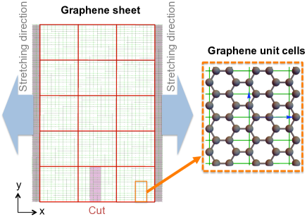
Figure 4: Schematic diagrams of graphene sheet and rectangular graphene unit cells. In this system, there are $3\times 5$ grids (colored red) where a cut may present or absent. Each grid consist of $10\times 16$ rectangular graphene unit cells (colored green) and each rectangular graphene unit cell consists of four carbon atoms.

We used the Sandia-developed open source LAMMPS (Large-scale Atomic/Molecular Massively Parallel Simulator) molecular dynamics (MD) simulation code to model graphene Lammps (2012). The carbon-carbon interactions are described by the AIREBO potential Stuart et al. (2000), which has been used previously to study graphene kirigami Qi et al. (2014). The cutoffs for the Lennard-Jones and the REBO term in AIREBO potential are chosen to be 2 Å and 6.8 Å, respectively. The graphene sheet of size $\sim 100\times 200$ Å consisting 2400 (9600 carbon atoms) rectangular graphene unit cells is shown in fig. 4. In the 15 grids (colored red), a cut of size $3\times 16$ rectangular graphene unit cells (colored green) is allowed to be present or absent. The graphene kirigami were stretched by applying loads at the $+x$ and $-x$ edges of the sheet. The atomic configurations were first relaxed by conjugate gradient energy minimization with a tolerance of $10^{-7}$. The graphene sheet was then relaxed at 4.2 K for 50 ps within the NVT (fixed number of atoms $N$, volume $V$, and temperature $T$) ensemble. Non-periodic conditions were applied in all three directions. After the NVT relaxation, the edge regions were moved at a strain rate of 0.01/ps, and the graphene sheet was stretched until fracture. This particular strain rate was chosen to save computational time as it has been shown that the fracture strain and fracture strength of graphene depend weakly on the strain rate, especially for low temperature Zhao and Aluru (2010). The 3D stress was calculated as the stress parallel to the loading direction times the simulation box size perpendicular to the plane and divided by the graphene effective thickness of 3.7 Å. Similar procedures have been used for other MD, DFT simulations and experiments Zhang et al. (2014); Hanakata et al. (2016a); Liu et al. (2007); Hanakata et al. (2016b); Lee et al. (2008).

As the cuts are allowed to be present in any of the $3\times 5$ grids there are $2^{15}=32768$ possible cut configurations, which we will refer to as the design space (or exploration space). Out of those, only 29791 configurations are not detached (no full cut along the $\hat{y}$ direction). Because the system is not periodic, translation symmetry is broken. The reflection symmetry is not broken and thus only about 1/4 of the possible configurations need to be simulated via MD.

II Machine learning performance and molecular dynamics precision

The root-mean-square error (RMSE) is given by,

$${\rm RMSE}=\sqrt{\frac{\sum^{m_{\rm test}}_{i=1}(y^{i}_{\rm test}-y^{i}_{\rm pred})^{2}}{m_{\rm test}}}$$ (1)

where $m_{\rm test}$ is the number of test datasets, $y_{\rm test}$ are the true values (obtained from MD) from the test dataset, and $y_{\rm pred}$ are the predicted values from a model.

Because of thermal fluctuations (non-zero temperature), the obtained yield strain or the yield stress of graphene from the MD simulations at 4.2 K will have some variation, which we will refer to as the MD precision. The MD precision (irreducible error) for the yield strain $\eta^{\varepsilon}$ can be approximated as root-mean-square deviation (RMSD),

$$\eta^{\varepsilon}=\sqrt{\frac{\sum^{T}_{i=1}(\varepsilon^{\rm y}_{i}-\overline{\varepsilon^{\rm y}})^{2}}{T}}\,,$$ (2)

where $T$ is the number of observations and $\overline{\varepsilon^{\rm y}}$ is the average of $\varepsilon^{\rm y}$ over $T$ observations which in this case are the different initial velocities (different initial conditions). The same formula is used for the yield stress $\eta^{\sigma}$. $\eta^{\varepsilon}$ is generally larger for systems with more cuts. To save computational time we randomly choose a configuration from systems having a cut density ranging from 0/15 to 12/15, calculate the RMSD from three different initial conditions, and then sum the RMSD of each cut. Note that cut densities of 13/15–15/15 are not considered because the structure is fully detached. For yield strain, the variability is more present at higher cut density and thus we sum the RMSD from cut densities ranging from 5/15 to 12/15. In addition to comparing RMSE and MD precision for evaluating the quality of a model, we quantify the performance of a model using an $R^{2}$ score on the test dataset given by

$$R^{2}=1-\frac{\sum^{m_{\rm test}}_{i=1}|y^{i}_{\rm test}-y^{i}_{\rm pred}|^{2}}{\sum^{m_{\rm test}}_{i=1}|y^{i}_{\rm test}-\frac{1}{m_{\rm test}}\sum^{m_{\rm test}}_{i=1}y^{i}_{\rm pred}|^{2}}\,.$$ (3)

III Machine learning

III.1 Hyperparameters for training

We used open-source machine learning packages to build the machine learning models. Specifically, we used TensorFlow r1.8 Abadi et al. (2015) for both the neural networks (NN) and convolutional neural networks (CNN) model and scikit-learn Pedregosa et al. (2011) for the ordinary least square regression model. The TensorFlow r1.8 was run on four CPUs and one NVDIA Tesla K40m GPU card.

We will denote $h$ as the number of neurons in a hidden layer $l$. In each layer the computation is given by

$$a^{(l+1)}=g(W^{(l)}a^{(l)}+b^{(l)}),$$ (4)

where $g$ is the rectified linear unit (ReLU) activation function, $a^{(l)}$, $b^{(l)}$, $W^{(l)}$ are the activations, bias, and the weights in a layer $l$. In CNN, we denote ‘h’ as the number of fully-connected-layers (FCL) and ‘f’ as the number of filters in a convolutional layer. So for a CNN model with 16 filters in first convolutional layer, 32 filters in second convolutional layer, 64 filters in third convolutional layer, and with a 64 FCL, we will denote is as CNN-f16-f32-f64-h64. For both NN and CNN, a learning rate of 0.0001 was used with a batch size of 200. The number of maximum epochs was set to 300. A larger learning rate, e.g 0.001, or smaller number total iteration number was found to have little effect on the performance. For the search algorithm CNN-f16-f32-f64-h64, a learning rate of 0.001 was used with a batch size of 100.

III.2 Convolutional Neural Networks Architecture

Figure 5: $R^{2}$ and RMSE for yield strain (a, b) and yield stress (c, d) as a function of number of neurons for NN or size of fully-connected layer for CNN for different number of grids. In general, an increasing number of neurons increases the model accuracy. It can be seen that the CNN models outperform the NN models.

The input to the convolutional neural networks (CNN) was a fixed-size $30\times 80$ grey image (0/1 grids). We followed an architecture similar to VGGNet Simonyan and Zisserman (2014). Specifically, the kernel size was fixed at $3\times 3$ with a stride of 1. Each convolutional layer was followed by a ReLU function and a max-pooling layer of size $2\times 2$ with a stride of 2. The same padding was used after the first convolutional layer to preserve the image size. We included one fully-connected layer of size ranging from 4 to 2024. As we performed regression, we did not include the ReLU function at the end of the final layer. The Adam optimizer was used to minimized the mean squared error.

In the supervised learning model, we split the 29,791 data samples into 80% for training, 10% for validation, and 10% for test dataset. The validation dataset is used to find better architectures (”hyperparameter tuning”, i.e. changing number of neurons or filters), and the test dataset is used to assess performance. In each model, the $R^{2}$ of the training dataset is slightly larger than the validation or test dataset, indicating that there is no overfitting problem. For instance, for CNN-f16-f32-f64-h64 the $R^{2}$ are 0.93, 0.91, 0.92, on training, validation, and test dataset respectively. The RMSE are 0.046, 0.056, 0.052 on training, validation, and test dataset respectively. We found that the deep CNN architecture with increasing number of filters from 16 to 64, similar to VGGNet architecture Simonyan and Zisserman (2014), performed the best compared to the wide CNN architectures or wide NNs. The performance comparison on the validation dataset is shown in fig. 5. In addition, we also include performance comparison for yield stress shown in fig. 5(c) and (d). Fig. 6 shows the CNN-f16-f32-f64-h64 fitness in predicting yield strain and yield stress on the test datasets.

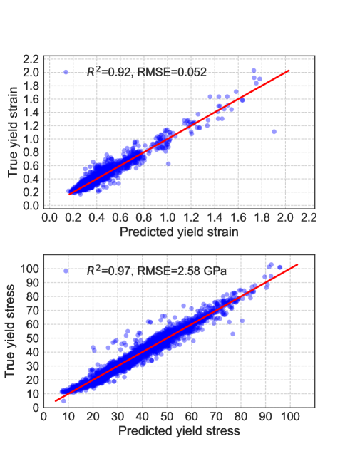
Figure 6: Plot of true values (test dataset) as a function of predicted value for (a) yield strain and (b) yield stress. Here, the CNN-f16-f32-f64-h64 model was used. The red line represents $y=x$ line.

IV Rotations in kirigami

Figure 7: Top and side views of three representative kirigamis.

The CNNs generate candidates with an extremely high yield strain compared to the pristine (cut-free) graphene sheet. Here we investigate the mechanisms enabling high stretchability, and focus on rotation mechanisms in a few kirigami structures as shown in fig. 7. First we compare a kirigami with typical centering cuts (fig. 7 I) and a kirigami with alternating edge cuts (fig. 7 II). Let the dimension of one cut be $c_{x}\times c_{y}$. We denote the “meeting point” in the middle segment where two ribbons are connected as a node, which are denoted by circles in fig. 7. Assuming there is no bond breaking, configuration I will have a maximum extension of $\approx 3c_{x}$ where the ribbons are connected by two nodes, whereas configuration II will have a maximum extension $\approx 7c_{x}$ as the ribbon is connected by one node. This additional degree of freedom (one fewer connecting node) enables configuration II to experience significantly more elastic stretching as compared to configuration I. As mentioned in the main text, the ML indeed found that the yield strain of configuration II is almost twice as large that of configuration I, as the alternating edge cut pattern effectively transforms the 2D membrane to quasi-1D membrane.

An additional consideration is how the closeness of the alternating edge cuts impacts the elastic stretchability. As can be seen by comparing configurations II and III in fig. 7, close packing of the alternating edge cuts allows increased stretchability. This is because, as seen from the side view, the ribbons need to rotate (twist) due to the applied tensile loading. Because the cuts are sparse in configuration III, the ribbons around the nodes are thick. In configuration II, the ribbons are thinner, which improves twisting and increases stretchability from 1.10 to 1.68.

V Linear model

In addition to the NN and CNN models, we applied a simple linear model to predict the yield strain and yield stress of the graphene kirigami. We formulate the objective functions (yield stress and strain) as

$$f(\boldsymbol{x})=\beta_{0}+\sum_{i}\beta_{i}x_{i}+\sum_{i\leq j}\beta_{ij}x_{i}x_{j}+\sum_{i\leq j\leq k}\beta_{ijk}x_{i}x_{j}x_{k}+\dots\,.$$ (5)

For $m$ samples, we can write Eq. 5 as a linear function $f(\boldsymbol{x})=\bf{X}^{T}\cdot\boldsymbol{\beta}$, where

$${\bf X}^{T}=\begin{pmatrix}1&x^{(1)}_{1}&\dots&x^{(1)}_{n}&x^{(1)}_{1}x^{(1)}_{2}&\dots\\ \vdots&\ddots&&&&\\ 1&x^{(m)}_{1}&\dots&x^{(m)}_{n}&x^{(\rm m)}_{1}x^{(m)}_{2}&\dots\end{pmatrix}\,,$$ (6)

and $\boldsymbol{\beta}^{T}=(\beta_{0},\beta_{1},\dots,\beta_{n},\beta_{12},\dots)$. In the machine learning language this is equivalent to applying features transformation to the input vectors. If the vector $\boldsymbol{x}$ is binary, the infinite series reduces into a finite series with $2^{n}$ terms. Symmetries and locality will further reduce the number of nonzero terms. For instance, in Ising and tight-binding models, interactions are usually considered up to the first or second nearest neighbors.

Since there is no theory that tells us the degree of the complexity, we will increase the degree of polynomial until a reasonable performance accuracy is achieved. We use the ordinary least squares (OLS) regression to describe the yield stress as a function of $\boldsymbol{x}$. For this regression model we use the 15 long array that distinguishes between cut and no cut in each grid as the input vector $\boldsymbol{x}$ and set the value of each component to be ‘1’ for no-cut and ‘-1’ for cut. For yield strain, a polynomial of degree 3 gives $R^{2}=0.76$ and ${\rm RMSE}=0.084$; for yield stress, a polynomial of degree 2 gives $R^{2}=0.93$ and root mean square error ${\rm RMSE}=4.1$ GPa.

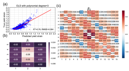
Figure 8: (a) Linear plot of true values (test data) as a function of predicted value for yield strain. (b) Learned first order parameter $\beta_{i}$ plotted in 2D arrays to match with the real space positions for yield strain. Here (1,1) is $\beta_{1}$, (1, 2) is $\beta_{2}$ and so on. (c) Learned matrix second order parameters (coupling interactions) $\beta_{ij}$ for yield strain. The red line represents $y=x$ line.

To gain a physical understanding of how the kirigami should be designed we plot the values of the parameters $\beta$. The first order parameters $\beta_{i}$ are negative, suggesting that yield strains will be higher when the materials have more cuts, as shown in fig. 8(b). The second order parameters $\beta_{ij}$ represent the pairwise ‘interaction coupling’, and these give better insights on how the kirigami should be designed in order to achieve high yield strains. From fig. 8(c), we see that the values $\beta_{ij}$ are lowest (most negative) between two neighbors along the $\vec{x}$ direction. On the other hand the coupling is positive between two neighbors along $\vec{y}$. For instance $\beta_{12}=0.01$ while $\beta_{16}=-0.02$. The regression results suggest that to achieve a high yield strain, cells (with a cut or no cut) of same type should be placed long the $\hat{y}$, while the opposite type should be placed right next to each other in the $\hat{x}$. This means the kirigami should have a line of cuts in $\hat{y}$ that alternate in the $\hat{x}$ direction. This resembles mechanical springs with two different constants that are connected in series. Overall, the first order parameters $\beta_{i}$ tell us that increasing cut density will result in higher strains; the second order parameters $\beta_{ij}$ gives further design principles on how the cuts should be arranged.

Figure 9: (a) Linear plot of true values (test data) as a function of predicted value for yield stress. (b) Learned first order parameter $\beta_{i}$ plotted in 2D arrays to match with the real space positions for yield stress. Here (1,1) is $\beta_{1}$, (1, 2) is $\beta_{2}$ and so on. (c) Learned matrix second order parameters (coupling interactions) $\beta_{ij}$ for yield stress. The red line represents $y=x$ line.

As shown in fig. 9(b), all first order parameters $\beta_{i}$ for yield stress are positive, suggesting that introducing cuts will lower the yield stress. From fig. 9(c), we see that the values are lowest (most negative) between two neighbors along the $\vec{y}$ direction. On the other hand the coupling is positive between two neighbors along $\vec{x}$. For instance $\beta_{12}=-1.5$ while $\beta_{16}=+1.5$. The regression results suggest that kirigami should have arrays of cuts (or no cuts) in $\hat{x}$ that alternate in the $\hat{y}$ direction. This resembles mechanical springs with two different constants that are connected in parallel. In contrast to nearest neighbor $\beta_{ij}$ of the yield strain, the nearest neighbor for yield strain is positive $\beta_{ij}>0$ along $\hat{x}$ while $\beta_{ij}<0$ when the $j$ element is not in the same $\hat{y}$.

We want to note that using series expansion works reasonably efficient for small system; however, for finer grids (or larger systems), the number of parameters will increase significantly as there will be $(n+d)!/(n!d!)\sim n^{d}/d$ of $\beta$ terms, where $d$ is the polynomial degree, $n$ is number of grids (features). Let us suppose we use one rectangular graphene unit cell as the size of one grid. Then, for a system size $\sim 100\times 200$ Å, the input size is $30\times 80=2400$ ($10\times 16$ rectangular graphene cells in each coarse grid). At a polynomial degree of 3, we will need $\sim 10^{9}$ parameters to fit.

In the series expansion approach, the 2D cut patterns are flattened into a 1D-array and thus some of the local spatial information are lost. Series expansion can be used to ‘recover’ the information of interactions between neighbors, but this approach becomes inefficient when the number of cells becomes large. This series expansion approach is computationally inefficient as we expect the interactions should be local. In principle, one could do series expansions to the nearest neighbors only; however, details of the potentials are not always known. For these reasons, the CNN is a more appropriate and scalable model as this deep learning is superior in recognizing edges in 2D motifs as well as performing down-sampling, which is very suitable for our problem. In the CNN, the 2D image (input) is convolved by a set of learnable filters and this allows the model to learn 2D motifs. An image passing through these filters then activates neurons which then classify (or rank) the cutting patterns to good or bad designs. This approach is more efficient than the series expansion approach as the CNN model is built based on learned 2D local motifs.

References

- Zirbel et al. (2013) S. A. Zirbel, R. J. Lang, M. W. Thomson, D. A. Sigel, P. E. Walkemeyer, B. P. Trease, S. P. Magleby, and L. L. Howell, Journal of Mechanical Design 135, 111005 (2013).
- Rafsanjani et al. (2018) A. Rafsanjani, Y. Zhang, B. Liu, S. M. Rubinstein, and K. Bertoldi, Science Robotics 3, eaar7555 (2018).
- Shyu et al. (2015) T. C. Shyu, P. F. Damasceno, P. M. Dodd, A. Lamoureux, L. Xu, M. Shlian, M. Shtein, S. C. Glotzer, and N. A. Kotov, Nature materials 14, 785 (2015).
- Blees et al. (2015) M. K. Blees, A. W. Barnard, P. A. Rose, S. P. Roberts, K. L. McGill, P. Y. Huang, A. R. Ruyack, J. W. Kevek, B. Kobrin, D. A. Muller, et al., Nature 524, 204 (2015).
- Qi et al. (2014) Z. Qi, D. K. Campbell, and H. S. Park, Phys. Rev. B 90, 245437 (2014).
- Hanakata et al. (2016a) P. Z. Hanakata, Z. Qi, D. K. Campbell, and H. S. Park, Nanoscale 8, 458 (2016a).
- Griffith and Eng (1921) A. A. Griffith and M. Eng, Phil. Trans. R. Soc. Lond. A 221, 163 (1921).
- Zhao and Aluru (2010) H. Zhao and N. Aluru, Journal of Applied Physics 108, 064321 (2010).
- Zhang et al. (2014) P. Zhang, L. Ma, F. Fan, Z. Zeng, C. Peng, P. E. Loya, Z. Liu, Y. Gong, J. Zhang, X. Zhang, et al., Nature communications 5, 3782 (2014).
- Jung et al. (2015) G. Jung, Z. Qin, and M. J. Buehler, Extreme Mechanics Letters 2, 52 (2015).
- Rakib et al. (2017) T. Rakib, S. Mojumder, S. Das, S. Saha, and M. Motalab, Physica B: Condensed Matter 515, 67 (2017).
- Dias et al. (2017) M. A. Dias, M. P. McCarron, D. Rayneau-Kirkhope, P. Z. Hanakata, D. K. Campbell, H. S. Park, and D. P. Holmes, Soft matter 13, 9087 (2017).
- Isobe and Okumura (2016) M. Isobe and K. Okumura, Scientific Reports 6, 24758 (2016).
- Rafsanjani and Bertoldi (2017) A. Rafsanjani and K. Bertoldi, Phys. Rev. Lett. 118, 084301 (2017).
- Moshe et al. (2018) M. Moshe, S. Shankar, M. J. Bowick, and D. R. Nelson, arXiv preprint arXiv:1801.08263 (2018).
- Masih Das et al. (2016) P. Masih Das, G. Danda, A. Cupo, W. M. Parkin, L. Liang, N. Kharche, X. Ling, S. Huang, M. S. Dresselhaus, V. Meunier, et al., ACS nano 10, 5687 (2016).
- Sigmund and Petersson (1998) O. Sigmund and J. Petersson, Structural optimization 16, 68 (1998).
- Jakiela et al. (2000) M. J. Jakiela, C. Chapman, J. Duda, A. Adewuya, and K. Saitou, Computer Methods in Applied Mechanics and Engineering 186, 339 (2000).
- Huang and Xie (2007) X. Huang and Y. Xie, Finite Elements in Analysis and Design 43, 1039 (2007).
- Gu et al. (2016) G. X. Gu, L. Dimas, Z. Qin, and M. J. Buehler, Journal of Applied Mechanics 83, 071006 (2016).
- Seko et al. (2015) A. Seko, A. Togo, H. Hayashi, K. Tsuda, L. Chaput, and I. Tanaka, Physical review letters 115, 205901 (2015).
- Sendek et al. (2017) A. D. Sendek, Q. Yang, E. D. Cubuk, K.-A. N. Duerloo, Y. Cui, and E. J. Reed, Energy & Environmental Science 10, 306 (2017).
- Onat et al. (2018) B. Onat, E. D. Cubuk, B. D. Malone, and E. Kaxiras, Physical Review B 97, 094106 (2018).
- Gu et al. (2018a) G. X. Gu, C.-T. Chen, and M. J. Buehler, Extreme Mechanics Letters 18, 19 (2018a).
- Behler and Parrinello (2007) J. Behler and M. Parrinello, Physical review letters 98, 146401 (2007).
- Behler (2011) J. Behler, The Journal of chemical physics 134, 074106 (2011).
- Cubuk et al. (2017a) E. D. Cubuk, B. D. Malone, B. Onat, A. Waterland, and E. Kaxiras, The Journal of chemical physics 147, 024104 (2017a).
- Cubuk et al. (2016) E. D. Cubuk, S. S. Schoenholz, E. Kaxiras, and A. J. Liu, The Journal of Physical Chemistry B 120, 6139 (2016).
- Schoenholz et al. (2017) S. S. Schoenholz, E. D. Cubuk, E. Kaxiras, and A. J. Liu, Proceedings of the National Academy of Sciences 114, 263 (2017).
- Cubuk et al. (2017b) E. Cubuk, R. Ivancic, S. Schoenholz, D. Strickland, A. Basu, Z. Davidson, J. Fontaine, J. Hor, Y.-R. Huang, Y. Jiang, et al., Science 358, 1033 (2017b).
- Carrasquilla and Melko (2017) J. Carrasquilla and R. G. Melko, Nature Physics 13, 431 (2017).
- Broecker et al. (2017) P. Broecker, J. Carrasquilla, R. G. Melko, and S. Trebst, Scientific reports 7, 8823 (2017).
- Gu et al. (2018b) G. X. Gu, C.-T. Chen, D. J. Richmond, and M. J. Buehler, Materials Horizons (2018b).
- Lammps (2012) Lammps, http://lammps.sandia.gov (2012).
- Simonyan and Zisserman (2014) K. Simonyan and A. Zisserman, CoRR abs/1409.1556 (2014).
- LeCun et al. (1998) Y. LeCun, L. Bottou, Y. Bengio, and P. Haffner, Proceedings of the IEEE 86, 2278 (1998).
- Note (1) Details of the specific GPU can be found in the SM.
- Hu et al. (2018) N. Hu, D. Chen, D. Wang, S. Huang, I. Trase, H. M. Grover, X. Yu, J. X. J. Zhang, and Z. Chen, Phys. Rev. Applied 9, 021002 (2018).
- Stuart et al. (2000) S. J. Stuart, A. B. Tutein, and J. A. Harrison, The Journal of chemical physics 112, 6472 (2000).
- Liu et al. (2007) F. Liu, P. Ming, and J. Li, Phys. Rev. B 76, 064120 (2007).
- Hanakata et al. (2016b) P. Z. Hanakata, A. Carvalho, D. K. Campbell, and H. S. Park, Physical Review B 94, 035304 (2016b).
- Lee et al. (2008) C. Lee, X. Wei, J. W. Kysar, and J. Hone, science 321, 385 (2008).
- Abadi et al. (2015) M. Abadi, A. Agarwal, P. Barham, E. Brevdo, Z. Chen, C. Citro, G. S. Corrado, A. Davis, J. Dean, M. Devin, S. Ghemawat, I. Goodfellow, A. Harp, G. Irving, M. Isard, Y. Jia, R. Jozefowicz, L. Kaiser, M. Kudlur, J. Levenberg, D. Mané, R. Monga, S. Moore, D. Murray, C. Olah, M. Schuster, J. Shlens, B. Steiner, I. Sutskever, K. Talwar, P. Tucker, V. Vanhoucke, V. Vasudevan, F. Viégas, O. Vinyals, P. Warden, M. Wattenberg, M. Wicke, Y. Yu, and X. Zheng, “TensorFlow: Large-scale machine learning on heterogeneous systems,” (2015), software available from tensorflow.org.
- Pedregosa et al. (2011) F. Pedregosa, G. Varoquaux, A. Gramfort, V. Michel, B. Thirion, O. Grisel, M. Blondel, P. Prettenhofer, R. Weiss, V. Dubourg, J. Vanderplas, A. Passos, D. Cournapeau, M. Brucher, M. Perrot, and E. Duchesnay, Journal of Machine Learning Research 12, 2825 (2011).