Construction of Kuranishi structures on the moduli spaces of pseudo-holomorphic disks: II

Abstract.

This is the second of a series of two articles in which we provide detailed and self-contained account of the construction of a system of Kuranishi structures on the moduli spaces of pseudo-holomorphic disks. Using the notion of obstruction bundle data introduced in [FOOO8], we give a systematic way of constructing a system of Kuranishi structures on the moduli spaces of pseudo-holomorphic disks which are compatible at the boundary and corners. More specifically, it defines a tree-like K-system in the sense of [FOOO6, Definition 21.9], [FOOO9, Definition 21.9]. The method given in this paper does not only simplify the description of the constructions in the earlier literature, but also is designed to provide a systematic utility tool for the construction of a system of Kuranishi structures in the future research. We also establish its uniqueness.

Aug 17th, 2018

1. Introduction

This article is a sequel to [FOOO8]. In the latter article, we gave a detailed construction of a Kuranishi structure on each individual moduli space of pseudo-holomorphic disks. In the present article we construct a system of Kuranishi structures on the moduli spaces of pseudo-holomorphic disks. More specifically, we will construct a tree-like K-system as defined in [FOOO6, Definition 21.9], [FOOO9, Definition 21.9]. Some explanation of such a construction has been given already in the earlier literature such as [FOOO2, FOOO4] focusing more on its applications to Lagrangian Floer theory. In this article and [FOOO8], we aim at focusing more on explaining minute details of the construction of a tree-like K-system. The present article adopts terminologies of [FOOO8]. In particular, systematically using the notion of obstruction bundle data introduced in [FOOO8], we give a systematic way of constructing a system of Kuranishi structures on the moduli spaces of pseudo-holomorphic disks. We also disseminate the construction into various pieces so that the outcome of each piece can be stated as an individual theorem which can be used by other researchers. Therefore the method we address in this paper does not only simplify the description of the constructions in the earlier literature, but also is designed to provide a systematic utility tool for the construction of a system of Kuranishi structures in the future research. We also establish uniqueness of the resulting system of Kuranishi structures (Theorem 2.21).

Let $(X,\omega)$ be a compact (or tame) symplectic manifold and $L$ its compact relatively spin Lagrangian submanifold. We consider the compactified moduli space $\mathcal{M}_{k+1}(X,L;\beta)$ of pseudo-holomorphic disks in $X$ bounding $L$ with $k+1$ boundary marked points in a given homology class $\beta\in H_{2}(X,L;{\mathbb{Z}})$. Our previous article [FOOO8] concerns the construction of a Kuranishi structure on this single moduli space individually.

In the present article we consider the whole collection of $\mathcal{M}_{k+1}(X,L;\beta)$ over $k,\,\beta\in H_{2}(X,L;{\mathbb{Z}})$ and construct a system of Kuranishi structures thereon so that the next equality holds as an isomorphism of spaces with Kuranishi structures, i.e., of K-spaces:

$$\partial\mathcal{M}_{k+1}(X,L;\beta)=\bigcup_{k_{1}+k_{2}=k+1} \bigcup_{i=1,\dots,k_{1}}\bigcup_{\beta_{1}+\beta_{2}=\beta}$$ (1.1)

$$\mathcal{M}_{k_{1}+1}(X,L;\beta_{1}){}_{{\rm ev}_{i}}\times_{{\rm ev}_{0}}\mathcal{M}_{k_{2}+1}(X,L;\beta_{2}).$$

Here the fiber product is taken over $L$ using the evaluation maps at the $i$-th and the $0$-th boundary marked points. Construction of such a system of Kuranishi structures is crucial for the construction of an $A_{\infty}$ structure associated to a Lagrangian submanifold. The issue of compatibility between various Kuranishi structures on various moduli spaces is more serious in the case of disks than in the case of closed Riemann surfaces, for example, in the study of Gromov-Witten invariants ([FOn]). This is the reason why the theory of open Gromov-Witten invariants takes a rather different shape from that of closed Gromov-Witten invariants. In fact, each $A_{\infty}$ operation $\mathfrak{m}_{k,\beta}$ itself, which is defined by a single moduli space $\mathcal{M}_{k+1}(X,L;\beta)$, depends on various choices involved, and so we have to construct the operators $\mathfrak{m}_{k,\beta}$ simultaneously in the way that they satisfy certain compatibility between one another. Only after that the totality of $\{\mathfrak{m}_{k,\beta}\}$ forms an $A_{\infty}$ structure that is well-defined up to certain homotopy equivalence.

In [FOOO8], we carried out the construction of a Kuranishi structure on each moduli space $\mathcal{M}_{k+1}(X,L;\beta)$ in the following order:

1. We define the notion of obstruction bundle data for each $\mathcal{M}_{k+1}(X,L;\beta)$. [FOOO8, Definition 5.1]. (See also Section 5 of this paper.)

2. We prove that we can extract a Kuranishi structure from the obstruction bundle data in a canonical way at the level of germs. ([FOOO8, Theorem 7.1])

3. We prove the existence of obstruction bundle data. ([FOOO8, Theorem 11.2])

In the present paper we perform the construction of a compatible system of Kuranishi structures in the following order:

1. We define the notion of a disk-component-wise system of obstruction bundle data. (Definition 5.1.) Such a system assigns obstruction bundle data to each $\mathcal{M}_{k+1}(X,L;\beta)$ for which we require certain compatibility conditions.

2. We prove that from each disk-component-wise system of obstruction bundle data we can extract a system of Kuranishi structures that is compatible with the decomposition of the boundary (1.1). (Theorem 5.3.)

3. We prove the existence of a disk-component-wise system of obstruction bundle data. (Theorem 5.4.)

Item (1) is the content of Section 5. We first define stratifications of the moduli spaces and their ambient ‘sets’ in Section 4. The stratifications are used to define the notion of compatible system, called disk-component-wise system, of obstruction bundle data in Section 5. Item (2) is carried out in Section 6. Item (3), the proof of existence of a disk-component-wise system, is technically the most involved one. It is carried out in Sections 7 and 8. In Section 9 we prove that the system of Kuranishi structures is independent of the choice of the system of obstruction bundle data from which it is extracted. We previously formulated the notion of pseudo-isotopy between two systems of Kuranishi structures in [FOOO6, Definition 21.19], [FOOO9, Definition 21.19]. We prove in Theorem 9.16 that if we are given two disk-component-wise systems of obstruction bundle data then the resulting systems of Kuranishi structures are pseudo-isotopic. (See Definition 2.20.) We also prove the resulting system of Kuranishi structures is independent of the choices of almost complex structures up to pseudo-isotopy, but depends only on $(X,\omega)$ and $(L,\sigma)$, where $\sigma$ is a relative spin structure on $L$. (See Theorems 2.8,2.21 and also Corollary 2.9. A similar result is proved in [DF] by a slightly different method.)

Remark 1.1.

This paper and [FOOO8] describe the case of moduli spaces of pseudo-holomorphic disks. However many of the constructions of this paper and [FOOO8] can be easily adapted to the case of other moduli spaces of pseudo-holomorphic curves. For example, the construction in [FOOO8] can be used to define a Kuranishi structure on the moduli space of marked stable maps (without boundary) of arbitrary genus. Therefore we can use it to define Gromov-Witten invariants of arbitrary genus. The argument of Section 9 of this paper together with [FOOO5, Corollary 14.28], [FOOO9, Proposition 14.13] can be used to prove their independence of various choices.

The way Kuranishi structure is associated to given obstruction bundle data provided in this paper and [FOOO8] is explicit and simple. (See (6.2).) Therefore when one wants to construct a Kuranishi structure with certain additional properties, one can do it by finding obstruction bundle data with corresponding additional properties. This method is useful in various applications. The fact that disk-component-wise-ness of the obstruction bundle data implies compatibility of Kuranishi structures with the isomorphism (1.1) (Theorem 5.3) is just one example. Other examples where such method can be applied are the compatibility with the forgetful map, the compatibility with a group action on the target space or anti-symplectic involution, cyclic symmetry of boundary marked points and etc.

Acknowledgments: KF, HO and KO thank IBS Center for Geometry and Physics for hospitality where a part of this work was done. The authors thank the anonymous referee for careful reading and useful comments.

2. Statement of the results

In this section, we precisely state the main result of this article. (We consider not only boundary marked points but also interior marked points.)

Situation 2.1.

$(X,\omega)$ is a symplectic manifold that is tame (at infinity). $(L,\sigma)$ is a compact Lagrangian submanifold of $X$ equipped with a relative spin structure $\sigma$. $J$ is an almost complex structure on $X$, which is tamed by $\omega$. $\beta\in H_{2}(X,L;{\mathbb{Z}})$. $\diamond$

Definition 2.2.

Let $k,\ell\in{\mathbb{Z}}_{\geq 0}$. We denote by $\mathcal{M}_{k+1,\ell}(X,L,J;\beta)$ the set of all $\sim$ equivalence classes of $((\Sigma,\vec{z},\vec{\mathfrak{z}}),u)$ with the following properties.

1. $\Sigma$ is a genus $0$ bordered curve with one boundary component that has only (boundary or interior) nodal singularities.

2. $\vec{z}=(z_{0},z_{1},\dots,z_{k})$ is a $(k+1)$-tuple of boundary marked points. We assume that they are distinct and are not nodal. Moreover we assume that they are numbered so that it respects the counter-clockwise cyclic ordering of the boundary.

3. $\vec{\mathfrak{z}}=({\mathfrak{z}}_{1},\dots,{\mathfrak{z}}_{\ell})$ are $\ell$ interior marked points. We assume that they are distinct and are not nodal.

4. $u:(\Sigma,\partial\Sigma)\to(X,L)$ is a continuous map which is pseudo-holomorphic on each irreducible component. The homology class $u_{*}([\Sigma,\partial\Sigma])$ is $\beta$.

5. $((\Sigma,\vec{z},\vec{\mathfrak{z}}),u)$ is stable in the sense of Definition 2.3 below.

We define the equivalence relation $\sim$ as follows. $((\Sigma,\vec{z},\vec{\mathfrak{z}}),u)\sim((\Sigma^{\prime},\vec{z}^{\,\prime},\vec{\mathfrak{z}^{\prime}}),u^{\prime})$ if there exists a homeomorphism $v:\Sigma\to\Sigma^{\prime}$ such that

1. $v$ is biholomorphic on each irreducible component.

2. $u^{\prime}\circ v=u$.

3. $v(\vec{z})=\vec{z}^{\,\prime}$. $v(\vec{\mathfrak{z}})=\vec{\mathfrak{z}}^{\prime}$.

Here and hereafter $v(\vec{\mathfrak{z}})=\vec{\mathfrak{z}}$ (resp. $v(\vec{z})=\vec{z}$) means $v({\mathfrak{z}}_{i})={\mathfrak{z}}_{i}$ (resp. $v(z_{i})=z_{i}$).

In case $\ell=0$, we write $\mathcal{M}_{k+1}(X,L,J;\beta)$ in place of $\mathcal{M}_{k+1,0}(X,L,J;\beta)$.

Definition 2.3.

Suppose $((\Sigma,\vec{z},\vec{\mathfrak{z}}),u)$ satisfies Definition 2.2 (1)(2)(3)(4). The group ${\rm Aut}^{+}((\Sigma,\vec{z},\vec{\mathfrak{z}}),u)$ of its extended automorphisms consists of homeomorphisms $v:\Sigma\to\Sigma$ such that:

1. $v$ is biholomorphic on each of the irreducible components.

2. $u\circ v=u$.

3. $v(\vec{z})=\vec{z}$ and there exists $\sigma\in{\rm Perm}(\ell)$ such that $(v({\mathfrak{z}}_{1}),\dots,v({\mathfrak{z}}_{\ell}))$ coincides with $({\mathfrak{z}}_{\sigma(1)},\dots,{\mathfrak{z}}_{\sigma(\ell)})$. Here ${\rm Perm}(\ell)$ is the group of permutations of the set $\{1,\dots,\ell\}$.

(iii) defines a group homomorphism ${\rm Aut}^{+}((\Sigma,\vec{z},\vec{\mathfrak{z}}),u)\to{\rm Perm}(\ell)$. The group of automorphisms ${\rm Aut}((\Sigma,\vec{z},\vec{\mathfrak{z}}),u)$ is its kernel.

The object $((\Sigma,\vec{z},\vec{\mathfrak{z}}),u)$ is said to be stable if ${\rm Aut}^{+}((\Sigma,\vec{z},\vec{\mathfrak{z}}),u)$ is a finite group.

Notation 2.4.

For ${\bf p}\in\mathcal{M}_{k+1,\ell}(X,L,J;\beta)$, we denote its representative by

$$((\Sigma_{\bf p},\vec{z}_{\bf p},\vec{\mathfrak{z}}_{\bf p}),u_{\bf p}).$$

In [FOOO2, Definition 7.1.42 and Theorem 7.1.43], we defined a topology on $\mathcal{M}_{k+1,\ell}(X,L,J;\beta)$ and proved that it is compact and Hausdorff with respect to this topology. We call this topology the stable map topology. The main result of this paper is as follows.

Theorem 2.5.

In Situation 2.1, there exists a tree-like K-system whose moduli spaces of operations are $\mathcal{M}_{k+1}(X,L,J;\beta)$.

A tree-like K-system is defined in Definition 2.18. More precisely it is the $\ell=0$ case of Definition 2.18. See [FOOO6, Definition 21.9], [FOOO9, Definition 21.9]. The notion of the moduli spaces of operations of a tree-like K-system is defined in [FOOO9, Condition 21.6 (III)].

We also remark that Theorems 2.5 and [FOOO6, Theorem 21.35 (1)], [FOOO9, Theorem 21.35 (1)] (using an algebraic lemma [FOOO1, Theorem 5.4.2]) imply the following:

Corollary 2.6.

([FOOO1, Theorem A]) To each $(X,\omega,J)$ and $(L,\sigma)$ as in Situation 2.1, we can associate a filtered $A_{\infty}$ structure on $H(L;\Lambda^{{\mathbb{R}}}_{\rm 0,nov})$.

We can prove well-defined-ness of the tree-like K-system in Theorem 2.5 and also its independence of the choice of almost complex structure $J$ as follows.

Situation 2.7.

Let $(X,\omega),(L,\sigma)$ be as in Situation 2.1. Suppose that $J_{1}$ and $J_{2}$ are compatible and tame almost complex structures on $X$. We take a smooth family of compatible and tame almost complex structures $\mathcal{J}=\{J_{s}\}$, $s\in[1,2]$ joining $J_{1}$ and $J_{2}$. $\diamond$

Theorem 2.8.

Suppose we are in Situation 2.7. By Theorem 2.5 we have a tree-like K-system whose moduli spaces of operations are $\mathcal{M}_{k+1}(X,L,J_{j};\beta)$, for $j=1,2$.

Then there exists a pseudo-isotopy of tree-like K-systems between them in the sense of [FOOO6, Definition 21.15] [FOOO9, Definition 21.15]. The moduli space of a $[1,2]$-parameterized family of $A_{\infty}$ operations are given by

$$\mathcal{M}_{k+1}(X,L,\mathcal{J};\beta;[1,2])=\bigcup_{s\in[1,2]}\{s\}\times\mathcal{M}_{k+1}(X,L,J_{s};\beta).$$

Theorems 2.8 and [FOOO6, Theorem 21.35 (3)], [FOOO9, Theorem 21.35 (3)] (using the algebraic lemma [FOOO1, Theorem 5.4.2] again) imply the following.

Corollary 2.9.

([FOOO1, Theorem A]) The filtered $A_{\infty}$ structure on $H(L;\Lambda^{{\mathbb{R}}}_{\rm 0,nov})$ given in Corollary 2.6 depends only on $(X,\omega)$ and $(L,\sigma)$ up to isomorphism. In particular, it is independent of the choices of almost complex structures and of obstruction bundle data up to isomorphism.

Remark 2.10.

1. The isomorphism of filtered $A_{\infty}$ structure in Corollary 2.9 means a filtered $A_{\infty}$ homomorphism that has an inverse. Note it may not be linear. (In that sense it is called sometimes a quasi-isomorphism.)

2. [FOOO1, Theorem A] is mostly the same result as Corollaries 2.6 and 2.9, but the ground ring in [FOOO1, Theorem A] is ${\mathbb{Q}}$. We used singular homology to construct a filtered $A_{\infty}$ structure over ${\mathbb{Q}}$ coefficients in place of ${\mathbb{R}}$ coefficients.

We can also prove the version with interior marked points. To state this version we need to prepare some notations. We first recall the following:

Definition 2.11.

We put $\mathfrak{G}=H_{2}(X,L;{\mathbb{Z}})$, $E(\beta)=\omega(\beta)$ and denote $\mu(\beta)$ by the Maslov index associated to $\beta\in\mathfrak{G}$.

Definition 2.12.

A decorated rooted ribbon tree is a pair $(\mathcal{T},\beta(\cdot))$ such that:

1. $\mathcal{T}$ is a connected tree. Let $C_{0}(\mathcal{T})$, $C_{1}(\mathcal{T})$ be the sets of all vertices and edges of $\mathcal{T}$, respectively.

2. For each ${\rm v}\in C_{0}(\mathcal{T})$ we fix a cyclic order of the set of edges containing ${\rm v}$. This is equivalent to fixing an isotopy type of an embedding of $\mathcal{T}$ to the plane ${\mathbb{R}}^{2}$. (Namely, the cyclic order of the edges is given by the orientation of the plane so that the edges are enumerated according to the counter clockwise orientation. We call it a ribbon structure at the vertex ${\rm v}$.)

3. $C_{0}(\mathcal{T})$ is divided into the set of exterior vertices $C_{0}^{{\rm ext}}(\mathcal{T})$ and the set of interior vertices $C_{0}^{{\rm int}}(\mathcal{T})$.

4. We fix one element of $C_{0}^{{\rm ext}}(\mathcal{T})$, which we call the root.

5. The valency of all the exterior vertices are $1$.

6. $\beta(\cdot):C_{0}^{{\rm int}}(\mathcal{T})\to\mathfrak{G}$ is a map. We require $E(\beta({\rm v}))\geq 0$. Moreover if $E(\beta({\rm v}))=0$ then $\beta({\rm v})$ is required to be $0\in H_{2}(X,L;{\mathbb{Z}})$.

7. (Stability) For each ${\rm v}\in C_{0}^{{\rm int}}(\mathcal{T})$ we assume that one of the following holds.

   1. $E(\beta({\rm v}))>0$.

   2. The valency of ${\rm v}$ is not smaller than $3$.

We denote by $\mathcal{G}(k+1,\beta)$ the set of all decorated rooted ribbon trees $(\mathcal{T},\beta(\cdot))$ such that:

1. $\#C_{0}^{{\rm ext}}(\mathcal{T})=k+1$.

2. $\sum_{{\rm v}\in C_{0}^{{\rm int}}(\mathcal{T})}(\beta({\rm v}))=\beta.$

We decompose the set of edges $C_{1}(\mathcal{T})$ into two types. If an edge ${\rm e}$ contains an exterior vertex, we call ${\rm e}$ an exterior edge. Otherwise we call ${\rm e}$ an interior edge. We denote by $C_{1}^{{\rm int}}(\mathcal{T})$, (resp. $C_{1}^{{\rm ext}}(\mathcal{T})$) the set of all interior (resp. exterior) edges.

Now we add interior marked points to $\mathcal{G}(k+1,\beta)$ and define the following set.

Definition 2.13.

The set $\mathcal{G}(k+1,\ell,\beta)$ consists of objects

$$\mathfrak{T}=(\mathcal{T},\beta(\cdot),l(\cdot))$$

with the following properties. We call $\mathfrak{T}$ a marked decorated rooted ribbon tree.

1. $(\mathcal{T},\beta(\cdot))$ satisfies Definition 2.12 (1)-(6), which is a part of the definition of the set $\mathcal{G}(k+1,\beta)$.

2. $l({\rm v})\subset\{1,\dots,\ell\}$ such that $\{1,\dots,\ell\}$ is a disjoint union of $\{l({\rm v})\mid{\rm v}\in C_{0}^{{\rm int}}(\mathcal{T})\}$.

3. Instead of Definition 2.12 (7) we assume the following. For each ${\rm v}\in C_{0}^{{\rm int}}(\mathcal{T})$ we assume that one of the following holds.

   1. $E(\beta({\rm v}))>0$.

   2. The valency of ${\rm v}$ is not smaller than $3$.

   3. $l({\rm v})\neq\emptyset$.

Using this, we incorporate the data of interior marked points into the definition of tree-like K-system ([FOOO6, Definition 21.9], [FOOO9, Definition 21.9]) as in Theorem 2.16. We also study isotopy etc. between them. For that purpose we include the parametrized version in the next definition.

Situation 2.14.

Let $(X,\omega),L$ be as in Situation 2.1 and $P$ a smooth compact oriented manifold with corners. We consider $\mathcal{J}=\{J_{t}\mid t\in P\}$, the smooth family of tame almost complex structures on $X$ parametrized by $P$. $\diamond$

Definition 2.15.

We put

$$\mathcal{M}_{k+1,\ell}(X,L,\mathcal{J};\beta)=\bigcup_{t\in P}\{t\}\times\mathcal{M}_{k+1,\ell}(X,L,J_{t};\beta).$$

We can define a stable map topology on this space in the same way as the case when $P$ is a point. There exists a map

$${\rm ev}_{P}:\mathcal{M}_{k+1,\ell}(X,L,\mathcal{J};\beta)\to P$$

which sends $\{t\}\times\mathcal{M}_{k+1,\ell}(X,L,J_{t};\beta)$ to $t$.

Theorem 2.16.

In Situation 2.14, there exists a system of Kuranishi structures on $\{\mathcal{M}_{k+1,\ell}(X,L,\mathcal{J};\beta)\mid k,\ell,\beta\}$ with the following properties:

(I) $\mathfrak{G}=H_{2}(X,L;{\mathbb{Z}})$, $E:\mathfrak{G}\to{\mathbb{R}}$ and $\mu:\mathfrak{G}\to{\mathbb{Z}}$ are as in Definition 2.11.

(II) Nothing to add.

(III)

$$({\rm ev}_{P},{\rm ev},{\rm ev}^{\rm int})= ({\rm ev}_{P},({\rm ev}_{0},\dots,{\rm ev}_{k}),({\rm ev}^{\rm int}_{1},\dots,{\rm ev}^{\rm int}_{\ell}))$$

$$:{\mathcal{M}}_{k+1,\ell}(X,L,\mathcal{J};\beta)\to P\times L^{k+1}\times X^{\ell}$$

is a strongly smooth map such that $({\rm ev}_{P},{\rm ev}_{0})$ is weakly submersive.

(IV) (Positivity of energy) We assume ${\mathcal{M}}_{k+1,\ell}(X,L,\mathcal{J};\beta)=\emptyset$ if $E(\beta)<0$.

(V) (Energy zero part) In case $E(\beta)=0$, we have ${\mathcal{M}}_{k+1,\ell}(X,L,\mathcal{J};\beta)=\emptyset$ unless $\beta=0$. In case $\beta=\beta_{0}=0$, we assume ${\mathcal{M}}_{k+1,\ell}(X,L,\mathcal{J};\beta_{0})=\emptyset$ if $k+1+2\ell<3$ and ${\mathcal{M}}_{k+1,\ell}(X,L,\mathcal{J};\beta_{0})=P\times L\times{\mathcal{M}}_{k+1,\ell}$ otherwise. Here ${\mathcal{M}}_{k+1,\ell}$ is the compactified moduli space of stable marked bordered curve of genus $0$ with one boundary component, $\ell$ interior marked points and $k+1$ boundary marked points.

(VI) (Dimension) The dimension of the moduli space $\mathcal{M}_{k+1,\ell}(X,L,\mathcal{J};\beta)$ is given by

$$\dim\mathcal{M}_{k+1,\ell}(X,L,\mathcal{J};\beta)=\mu(\beta)+\dim L+k-2+2\ell+\dim P.$$ (2.1)

(VII) (Orientation) ${\mathcal{M}}_{k+1,\ell}(X,L,\mathcal{J};\beta)$ is oriented.

(VIII) (Gromov compactness) For any $E_{0}$ the set

$$\{\beta\in\mathfrak{B}\mid\exists k\,\,\exists\ell\,\,\,{\mathcal{M}}_{k+1,\ell}(X,L,\mathcal{J};\beta)\neq\emptyset,\,\,E(\beta)\leq E_{0}\}$$ (2.2)

is a finite set.

(IX) (Compatibility at the boundary) The normalized boundary of ${\mathcal{M}}_{k+1,\ell}(X,L,\mathcal{J};\beta)$ is decomposed to the disjoint union of fiber products as follows.

$$\widehat{\partial}{\mathcal{M}}_{k+1,\ell}(X,L,\mathcal{J};\beta)$$ (2.3)

$$\cong\coprod_{\beta_{1},\beta_{2},k_{1},k_{2},i,l_{1},l_{2}}(-1)^{\epsilon}{\mathcal{M}}_{k_{1}+1,\#l_{1}}(X,L,\mathcal{J};\beta_{1})$$

$$\qquad\qquad\qquad\qquad\qquad\qquad\,\,{}_{({\rm ev}_{P},{\rm ev}_{i})}\times_{({\rm ev}_{P},{\rm ev}_{0})}{\mathcal{M}}_{k_{2}+1,\#l_{2}}(X,L,\mathcal{J};\beta_{2})$$

$$\qquad\qquad\cup{\mathcal{M}}_{k+1,\ell}(X,L,\mathcal{J}|_{\widehat{\partial}P};\beta)$$

where the union of the first term of the right hand side is taken over $\beta_{1},\beta_{2},k_{1},k_{2}$ such that $\beta_{1}+\beta_{2}=\beta$, $k_{1}+k_{2}=k+1$, $i=1,\dots,k_{1}$ and $l_{1},l_{2}$ that are subsets of $\{1,\dots,\ell\}$ such that $l_{1}\cap l_{2}=\emptyset$, $l_{1}\cup l_{2}=\{1,\dots,\ell\}$. $\mathcal{J}|_{\widehat{\partial}P}$ is the restriction of the family $\mathcal{J}$ to the normalized boundary of $P$.

We refer [FOOO6, (21.15),(21.16)], [FOOO9, (21.15),(21.16)] for the description of the sign ${\epsilon}$. (c.f. [FOOO2, Section 8.5]) See also [FOOO6, Remark 16,2], [FOOO9, Remark 16,2] for the order of fiber product and orientation etc.

This isomorphism is compatible with orientation. It is compatible also with the evaluation maps. (Compatibility with the evaluation maps at the boundary marked points is the same as that of [FOOO6, Formula (21.8)], [FOOO9, Formula (21.8)]. Compatibility at the interior marked points can be formulated in the similar way by using the indexing set $l_{1}\sqcup l_{2}=\{1,\dots,\ell\}$.)

(X) (Corner compatibility isomorphism) Let $\widehat{S}_{m}({\mathcal{M}}_{k+1,\ell}(X,L,\mathcal{J};\beta))$ be the normalized corner of the K-space ${\mathcal{M}}_{k+1,\ell}(X,L,\mathcal{J};\beta)$ in the sense of [FOOO6, Definition 24.17], [FOOO9, Definition 24.18]. Then it is isomorphic to the disjoint union of

$$\prod_{(\mathcal{T},\beta(\cdot),l(\cdot))}{\mathcal{M}}_{k_{\rm v}+1,\#l({\rm v})}(X,L,\mathcal{J}|_{\widehat{S}_{m^{\prime}}P};\beta({\rm v})).$$ (2.4)

Here the union is taken over all $(\mathcal{T},\beta(\cdot),l(\cdot))\in\mathcal{G}(k+1,\ell,\beta)$, $m^{\prime}$ such that $\#C_{1}^{{\rm int}}(\mathcal{T})+m^{\prime}=m$, and $\prod_{(\mathcal{T},\beta(\cdot),l(\cdot))}$ means a fiber product defined in Definition 4.1. $\mathcal{J}|_{\widehat{S}_{m^{\prime}}P}$ is the restriction of the family $\mathcal{J}$ to the codimension $m^{\prime}$ normalized corner $\widehat{S}_{m^{\prime}}P$ of $P$. We call the isomorphism

$$\widehat{S}_{m}({\mathcal{M}}_{k+1,\ell}(X,L,\mathcal{J};\beta))$$ (2.5)

$$\xrightarrow{\sim}\coprod_{\begin{subarray}{c}(\mathcal{T},\beta(\cdot),l(\cdot))\in\mathcal{G}(k+1,\ell,\beta),\\ m^{\prime}\end{subarray}}\prod_{(\mathcal{T},\beta(\cdot),l(\cdot))}{\mathcal{M}}_{k_{\rm v}+1,\#l({\rm v})}(X,L,\mathcal{J}|_{\widehat{S}_{m^{\prime}}P};\beta({\rm v}))$$

the corner compatibility isomorphism. It is compatible with the evaluation maps.

(XI) (Consistency of corner compatibility isomorphisms) We iterate the construction of normalized corner and obtain a space $\widehat{S}_{m_{2}}(\widehat{S}_{m_{1}}({\mathcal{M}}_{k+1,\ell}(X,L,\mathcal{J};\beta)))$. Condition (X) implies that $\widehat{S}_{m_{2}}(\widehat{S}_{m_{1}}({\mathcal{M}}_{k+1,\ell}(X,L,\mathcal{J};\beta)))$ is a disjoint union of $(m^{\prime}+m_{1}+m_{2})!/m^{\prime}!m_{1}!m_{2}!$ copies of (2.4), where the union is taken over all $(\mathcal{T},\beta(\cdot),l(\cdot))\in\mathcal{G}(k+1,\ell,\beta)$ such that $\#C_{1}^{{\rm int}}(\mathcal{T})=m_{1}+m_{2}$, $m=m^{\prime}+m_{1}+m_{2}$.

The map

$$\pi_{m_{2},m_{1}}:\widehat{S}_{m_{2}}(\widehat{S}_{m_{1}}({\mathcal{M}}_{k+1,\ell}(X,L,\mathcal{J};\beta)))\to\widehat{S}_{m_{1}+m_{2}}({\mathcal{M}}_{k+1,\ell}(X,L,\mathcal{J};\beta))$$

in [FOOO6, Proposition 24.16], [FOOO9, Proposition 24.17] is identified with the identity map on each component of (2.4).

(XII) (Exchange symmetry of the interior marked points) There exists an action of symmetric group ${\rm Perm}(\ell)$ on the K-space ${\mathcal{M}}_{k+1,\ell}(X,L,\mathcal{J};\beta)$, whose underlying action on the topological space ${\mathcal{M}}_{k+1,\ell}(X,L,\mathcal{J};\beta)$ is by exchanging the interior marked points. This action is compatible with the evaluation map and the corner compatibility isomorphisms given in (X)(XI). It is orientation preserving.

Remark 2.17.

The notion of a normalized boundary and normalized corners of a manifold (or an orbifold) with corners are defined in [FOOO9, Definitions 8.4 and 24.18] [FOOO9, Lemma-Definition 8.8]. For example the normalized boundary of the subspace $\{(x,y)\mid x,y\in{\mathbb{R}},x,y\geq 0\}$ of ${\mathbb{R}}^{2}$ is a disjoint union of two half lines $\{x\mid x\geq 0\}\sqcup\{y\mid y\geq 0\}$. Two points of the normalized boundary, $x=0$ in the first summand and $y=0$ in the second summand, become the same point in the usual boundary. A normalized boundary of a manifold with corners becomes a manifold with corners. (This is not the case for the usual boundary.)

Definition 2.18.

We call the system satisfying (I)-(XII) of Theorem 2.16 with $P=$ point, a tree-like K-system with interior marked points.

Theorem 2.16 implies the existence of bulk deformations of Lagrangian Floer cohomology. (See [FOOO1, Subsection 3.8.5].) Namely it induces

$$\mathfrak{q}:H(X;\Lambda^{{\mathbb{R}}}_{\rm 0,nov})\to HH(H(L;\Lambda^{{\mathbb{R}}}_{\rm 0,nov}),H(L;\Lambda^{{\mathbb{R}}}_{\rm 0,nov}))$$ (2.6)

from the cohomology of the ambient space $X$ to the Hochschild cohomology of the filtered $A_{\infty}$ algebra in Corollary 2.6. More precisely (2.6) is a filtered $L_{\infty}$ homomorphism, where the $L_{\infty}$ structure of the domain is trivial and the $L_{\infty}$ structure of the target is induced by the Gerstenhaber bracket. See [FOOO1, Theorem Y and Theorem 3.8.32], [FOOO2, Corollary 7.4.40] for the precise statement. There is a similar well-definedness statement as Theorem 2.8 in the situation of Theorem 2.16. It implies that the map (2.6) is independent of the choices up to homotopy of filtered $L_{\infty}$ homomorphism.

Remark 2.19.

The map $\mathfrak{q}$ is called the closed-open map. It is a ring homomorphism when we use quantum cup product on $H(X;\Lambda^{{\mathbb{R}}}_{\rm 0,nov})$. See [FOOO3, Subsection 4.7] for various works related to this map.

Definition 2.20.

([FOOO6, Definition 21.15], [FOOO9, Definition 21.15]) A pseudo isotopy between two tree-like K-systems with interior marked points is a system satisfying (I)-(XII) of Theorem 2.16 with $P=[1,2]$ such that its restriction to $1$ and $2$ becomes the given two tree-like K-systems with interior marked points.

Theorem 2.21.

Any two tree-like K-systems with interior marked points obtained by Theorem 2.16 with $P=$ point are pseudo-isotopic.

The proofs of Theorems 2.5, 2.8 and 2.16, 2.21 occupy the rest of this article.

3. Obstruction bundle data: Review

We first review the definition of obstruction bundle data in [FOOO8].

We considered the set ${\mathcal{X}}_{k+1,\ell}(X,L;\beta)$ of all isomorphism classes of $((\Sigma,\vec{z},\vec{\mathfrak{z}}),u)$ which satisfy the same condition as in Definition 2.2 except we do not require $u$ to be pseudo-holomorphic. We require $u$ to be continuous and of $C^{2}$ class on each irreducible component. (See [FOOO8, Definition 4.2].) This is a set which contains ${\mathcal{M}}_{k+1,\ell}(X,L,J;\beta)$ set-theoretically. We emphasize that we do not put structures on ${\mathcal{X}}_{k+1,\ell}(X,L;\beta)$ such as topology. We use partial topology of the pair $({\mathcal{X}}_{k+1,\ell}(X,L;\beta),{\mathcal{M}}_{k+1,\ell}(X,L,J;\beta))$: It assigns $B_{\epsilon}(\mathcal{X},{\bf p})\subset{\mathcal{X}}_{k+1,\ell}(X,L;\beta)$ to each ${\bf p}\in{\mathcal{M}}_{k+1,\ell}(X,L,J;\beta)$ and $\epsilon>0$. Here $B_{\epsilon}(\mathcal{X},{\bf p})$ is the set of ${\bf x}\in{\mathcal{X}}_{k+1,\ell}(X,L;\beta)$ such that $\bf x$ is $\epsilon$-close to $\bf p$. See [FOOO8, Definition 4.12] for the definition that ‘$\bf x$ is $\epsilon$-close to $\bf p$,’ and [FOOO8, Definition 4.1] for the definition of the notion of partial topology and [FOOO8, Subsection 4.3] for the definition of the partial topology in the case of the pair $({\mathcal{X}}_{k+1,\ell}(X,L;\beta),{\mathcal{M}}_{k+1,\ell}(X,L,J;\beta))$. A subset

$$\mathscr{U}_{\bf p}\subset{\mathcal{X}}_{k+1,\ell}(X,L;\beta)$$

is called a neighborhood of ${\bf p}$ in ${\mathcal{X}}_{k+1,\ell}(X,L;\beta)$ if it contains $B_{\epsilon}(\mathcal{X},{\bf p})$ for sufficiently small $\epsilon>0$. Now we recall:

Definition 3.1.

([FOOO8, Definition 5.1]) Obstruction bundle data of (or for) the moduli space ${\mathcal{M}}_{k+1,\ell}(X,L,J;\beta)$ assign to each ${\bf p}\in{\mathcal{M}}_{k+1,\ell}(X,L,J;\beta)$ a neighborhood $\mathscr{U}_{\bf p}$ of ${\bf p}$ in ${\mathcal{X}}_{k+1,\ell}(X,L;\beta)$ and an object $E_{\bf p}(\bf x)$ to each ${\bf x}\in\mathscr{U}_{\bf p}$ . We require that they have the following properties.

1. We put ${\bf x}=((\Sigma_{\bf x},\vec{z}_{\bf x},\vec{\mathfrak{z}}_{\bf x}),u_{\bf x})$. Then $E_{\bf p}({\bf x})$ is a finite dimensional linear subspace of the set of $C^{2}$ sections

   $$E_{\bf p}({\bf x})\subset C^{2}(\Sigma_{\bf x};u_{\bf x}^{*}TX\otimes\Lambda^{0,1}),$$

   whose supports are away from nodal or marked points and the boundary.

2. (Smoothness) $E_{\bf p}({\bf x})$ depends smoothly on ${\bf x}$ as defined in [FOOO8, Definition 8.7].

3. (Transversality) $E_{\bf p}({\bf x})$ satisfies the transversality condition as in [FOOO8, Definition 5.5].

4. (Semi-continuity) $E_{\bf p}({\bf x})$ is semi-continuous on ${\bf p}$ as defined in [FOOO8, Definition 5.2].

5. (Invariance under extended automorphisms) $E_{\bf p}({\bf x})$ is invariant under the extended automorphism group of ${\bf x}$ as in [FOOO8, Condition 5.6].

6. (Effectivity) The action of ${\rm Aut}({\bf p})$ on $(D_{u_{\bf p}}\overline{\partial})^{-1}(E_{\bf p})/{\mathfrak{aut}}(\Sigma_{\bf p},\vec{z}_{\bf p},\vec{\mathfrak{z}}_{\bf p})$ is effective.

In [FOOO8, Theorem 7.1] we associated a Kuranishi structure of ${\mathcal{M}}_{k+1,\ell}(X,L,J;\beta)$ to the obstruction bundle data, which is determined canonically in the sense of germ of Kuranishi structures.

4. Stratification of the moduli space

In the next section, Section 5, we spell out the condition of the obstruction bundle data which enables us to relate those Kuranishi structures on ${\mathcal{M}}_{k+1,\ell}(X,L,J;\beta)$ one another on the boundaries and the corners by appropriate fiber products. In this section, we describe stratifications of ${\mathcal{M}}_{k+1,\ell}(X,L,J;\beta)$, ${\mathcal{X}}_{k+1,\ell}(X,L;\beta)$, which we use for this purpose.

Let $(\mathcal{T},\beta(\cdot),\ell(\cdot))\in\mathcal{G}(k+1,\ell,\beta)$. We define the fiber product (2.4) as follows. We first consider the direct product

$$\prod_{{\rm v}\in C_{0}^{{\rm int}}(\mathcal{T})}{\mathcal{M}}_{k_{\rm v}+1,\#l({\rm v})}(X,L,J;\beta({\rm v})).$$ (4.1)

We will define a map

$$\mathcal{EV}:\prod_{{\rm v}\in C_{0}^{{\rm int}}(\mathcal{T})}{\mathcal{M}}_{k_{\rm v}+1,\#l({\rm v})}(X,L,J;\beta({\rm v}))\to(L\times L)^{\#C_{1}^{{\rm int}}(\mathcal{T})}$$

below. Here the target is a direct product of $\#C_{1}^{{\rm int}}(\mathcal{T})$ copies of $L\times L$.

Let ${\rm e}\in C_{1}^{{\rm int}}(\mathcal{T})$ and $\{t({\rm e}),s({\rm e})\}=\partial{\rm e}$. Here we require the vertex $t({\rm e})$ to be in the same connected component of $\mathcal{T}\setminus\{s({\rm e})\}$ as the root $\mathfrak{v}_{0}$. (See Figure 1.) For each ${\rm v}\in C_{0}^{{\rm int}}(\mathcal{T})$ there is a unique edge ${\rm e}_{0}(\rm v)\in C_{0}(\mathcal{T})$ adjacent to ${\rm v}$ such that ${\rm e}_{0}(\rm v)$ is contained in the same connected component of $\mathcal{T}\setminus{\rm v}$ as the root. Let ${\rm e}_{1}({\rm v}),\dots,{\rm e}_{k_{\rm v}}({\rm v})$ be the edges containing ${\rm v}$ such that $({\rm e}_{0}({\rm v}),{\rm e}_{1}({\rm v}),\dots,{\rm e}_{k_{\rm v}}({\rm v}))$ respects the counterclockwise order induced by the ribbon structure. By definition

$${\rm e}={\rm e}_{0}(s({\rm e})).$$

Let $k_{{\rm e}}$ be a positive integer such that

$${\rm e}={\rm e}_{k_{{\rm e}}}(t({\rm e})).$$

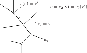
Figure 1. $s({\rm e})$ and $t({\rm e})$

Let $\vec{\bf p}=({\bf p}_{{\rm v}})_{{\rm v}\in C_{0}^{{\rm int}}}$ be an element of (4.1). We put

$$\mathcal{EV}_{{\rm e}}(\vec{\bf p})=({\rm ev}_{0}({\bf p}_{s({\rm e})}),{\rm ev}_{k_{\rm e}}({\bf p}_{t({\rm e})}))\in L\times L$$

and

$$\mathcal{EV}=(\mathcal{EV}_{{\rm e}}(\vec{\bf p}))_{{\rm e}\in C_{1}^{{\rm int}}(\mathcal{T})}.$$

Definition 4.1.

We put

$$\prod_{(\mathcal{T},\beta(\cdot),l(\cdot))}{\mathcal{M}}_{k_{\rm v}+1,\#l({\rm v})}(X,L,J;\beta({\rm v}))$$

$$=\prod_{{\rm v}\in C_{0}^{{\rm int}}(\mathcal{T})}{\mathcal{M}}_{k_{\rm v}+1,\#l({\rm v})}(X,L,J;\beta({\rm v})){}_{\mathcal{EV}}\times\Delta^{\#C_{1}^{{\rm int}}(\mathcal{T})}.$$

Here $\Delta\subset L\times L$ is the diagonal. In other words, it is the set of all elements $\vec{\bf p}=({\bf p}_{{\rm v}})_{{\rm v}\in C_{0}^{{\rm int}}}({\mathcal{T}})$ of (4.1) such that

$${\rm ev}_{0}({\bf p}_{s({\rm e})})={\rm ev}_{k_{\rm e}}({\bf p}_{t({\rm e})})$$ (4.2)

for all ${\rm e}\in C_{1}^{{\rm int}}(\mathcal{T})$. To simplify the notation we write

$${\mathcal{M}}_{k+1,\ell}(X,L,J;\beta)(\mathfrak{T}):=\prod_{(\mathcal{T},\beta(\cdot),l(\cdot))}{\mathcal{M}}_{k_{\rm v}+1,\#l({\rm v})}(X,L,J;\beta({\rm v}))$$ (4.3)

with $\mathfrak{T}=(\mathcal{T},\beta(\cdot),l(\cdot))$.

Lemma 4.2.

There exists a homeomorphism onto its image

$${\mathcal{M}}_{k+1,\ell}(X,L,J;\beta)(\mathfrak{T})\to{\mathcal{M}}_{k+1,\ell}(X,L,J;\beta).$$ (4.4)

Proof.

Let $\vec{\bf p}=({\bf p}_{{\rm v}})_{{\rm v}\in C_{0}^{{\rm int}}}(\mathcal{T})$ be an element of (4.1) satisfying (4.2). We put ${\bf p}_{{\rm v}}=((\Sigma_{{\rm v}},\vec{z}_{{\rm v}},\vec{\mathfrak{z}}_{{\rm v}}),u_{\rm v})$. We glue $(\Sigma_{{\rm v}},\vec{z}_{{\rm v}},\vec{\mathfrak{z}}_{{\rm v}})$ to obtain $(\Sigma,\vec{z},\vec{\mathfrak{z}})$ as follows. Consider the disjoint union $\bigcup\Sigma_{{\rm v}}$. For each ${\rm e}\in C_{1}^{{\rm int}}(\mathcal{T})$ we identify the $0$-th (boundary) marked point of $\Sigma_{s({\rm e})}$ with $k_{\rm e}$-th (boundary) marked point of $\Sigma_{t({\rm e})}$. We thus obtain $\Sigma$. We define $k+1$-boundary marked points $\vec{z}$ of $\Sigma$ as follows. Let $i\in\{0,\dots,k\}$. We consider the $i$-th exterior vertex ${\rm v}_{i}$ of $\mathcal{T}$. Let ${\rm e}_{i}$ be the edge containing it and ${\rm v}^{\prime}_{i}$ be the other vertex contained in ${\rm e}_{i}$. Suppose ${\rm e}_{i}={\rm e}_{j}({\rm v}^{\prime}_{i})$. Then $z_{i}$ is the $j$-th boundary marked point of $\Sigma_{{\rm v}^{\prime}_{i}}$. We define interior marked points $\vec{\mathfrak{z}}_{{\rm v}}$ using $l(\cdot)$ in a similar way.

We define $u:\Sigma\to X$ so that $u|_{\Sigma_{\rm v}}=u_{\rm v}$. By (4.2) $u$ is continuous. It is easy to see that $((\Sigma,\vec{z},\vec{\mathfrak{z}}),u)$ represents an element of ${\mathcal{M}}_{k+1,\ell}(X,L,J;\beta)$. We have thus defined a map (4.4). By the definition of stable map topology (see [FOOO2, Definition 7.1.39]) this is a homeomorphism onto its image. ∎

Note ${\mathcal{M}}_{k+1,\ell}(X,L,J;\beta)(\mathfrak{T})$ is compact. So its image in ${\mathcal{M}}_{k+1,\ell}(X,L,J;\beta)$ is a closed subset.

Let

$${\mathcal{M}}^{\circ}_{k+1,\ell}(X,L,J;\beta)$$

be a subset of ${\mathcal{M}}_{k+1,\ell}(X,L,J;\beta)$ consisting of those elements $((\Sigma,\vec{z},\vec{\mathfrak{z}}),u)$ whose domain $\Sigma$ contains only one irreducible disk component. We put

$${\mathcal{M}}^{\circ}_{k+1,\ell}(X,L,J;\beta)(\mathfrak{T})$$ (4.5)

$$:=\prod_{{\rm v}\in C_{0}^{{\rm int}}(\mathcal{T})}{\mathcal{M}}^{\circ}_{k_{\rm v}+1,\#l({\rm v})}(X,L,J;\beta({\rm v})){}_{\mathcal{EV}}\times\Delta^{\#C_{1}^{{\rm int}}(\mathcal{T})},$$

which is a subset of ${\mathcal{M}}_{k+1,\ell}(X,L,J;\beta)(\mathfrak{T})$. We regard it as a subset of ${\mathcal{M}}_{k+1,\ell}(X,L,J;\beta)$ by Lemma 4.2. The next lemma is immediate from the construction.

Lemma 4.3.

${\mathcal{M}}_{k+1,\ell}(X,L,J;\beta)$ is a disjoint union of ${\mathcal{M}}^{\circ}_{k+1,\ell}(X,L,J;\beta)(\mathfrak{T})$ over various $\mathfrak{T}\in\mathcal{G}(k+1,\ell,\beta)$.

Let $(\mathcal{T},\beta(\cdot),l(\cdot))\in\mathcal{G}(k+1,\ell,\beta)$ and $\rm e$ its interior edge. We define $(\mathcal{T}^{\prime},\beta^{\prime}(\cdot),l^{\prime}(\cdot))\in\mathcal{G}(k+1,\ell,\beta)$ as follows:

1. $\mathcal{T}^{\prime}$ is obtained by contracting ${\rm e}$ to a point in $\mathcal{T}$.

2. We have $\beta^{\prime}({\rm v})=\beta({\rm v})$ if ${\rm v}$ is not a vertex corresponding to ${\rm e}$, and $\beta^{\prime}({\rm v})=\beta({\rm v}_{1})+\beta({\rm v}_{2})$ if ${\rm v}$ is the vertex corresponding to the contracted edge ${\rm e}$ with $\partial{\rm e}=\{{\rm v}_{1},{\rm v}_{2}\}$.

3. We set $l^{\prime}({\rm v})=l({\rm v})$ if ${\rm v}\in C_{0}^{\rm int}(\mathcal{T})$ is neither ${\rm v}_{1}$ nor ${\rm v}_{2}$ (vertices of ${\rm e}$). (Note such ${\rm v}$ can be regarded as an interior vertex of $\mathcal{T}^{\prime}$.) We also put $l^{\prime}({\rm v})=l({\rm v}_{1})\cup l({\rm v}_{2})$ if ${\rm v}$ is the new vertex obtained by collapsing ${\rm e}$.

We say $(\mathcal{T}^{\prime},\beta^{\prime}(\cdot),l^{\prime}(\cdot))$ is obtained from $(\mathcal{T},\beta(\cdot),l(\cdot))$ by an edge contraction. We say $\mathfrak{T}^{\prime}\geq\mathfrak{T}$ if $\mathfrak{T}^{\prime}$ is obtained from $\mathfrak{T}$ by finitely many times of edge contractions. (The case $\mathfrak{T}=\mathfrak{T}^{\prime}$ is included.)

The next lemma is obvious from definition.

Lemma 4.4.

Suppose ${\mathcal{M}}_{k+1,\ell}(X,L,J;\beta)(\mathfrak{T})$ is nonempty. Then $\mathfrak{T}\leq\mathfrak{T}^{\prime}$ if and only if ${\mathcal{M}}_{k+1,\ell}(X,L,J;\beta)(\mathfrak{T})\subseteq{\mathcal{M}}_{k+1,\ell}(X,L,J;\beta)(\mathfrak{T}^{\prime})$.

We also remark the following.

Lemma 4.5.

Let ${\bf p}\in{\mathcal{M}}^{\circ}_{k+1,\ell}(X,L,J;\beta)(\mathfrak{T})\subset{\mathcal{M}}_{k+1,\ell}(X,L,J;\beta)$. Then ${\bf p}$ is a point in the codimension $m$ corner with respect to the Kuranishi structure of ${\mathcal{M}}_{k+1,\ell}(X,L,J;\beta)$ if and only if $\mathfrak{T}$ has at least $m$ interior edges.

Proof.

Let ${\bf p}=((\Sigma,\vec{z},\vec{\mathfrak{z}}),u)=({\bf p}_{{\rm v}})_{{\rm v}\in C_{0}^{{\rm int}}(\mathcal{T})}$. By construction, the Kuranishi neighborhoods of ${\bf p}$ is diffeomorphic to the fiber product of the Kuranishi neighborhoods of various ${\bf p}_{{\rm v}}$ in ${\mathcal{M}}^{\circ}_{k_{\rm v}+1,\#l({\rm v})}(X,L,J;\beta({\rm v}))$ times $[0,1)^{\#C_{1}^{{\rm int}}(\mathcal{T})}$. The Kuranishi neighborhood of ${\bf p}_{{\rm v}}$ has no boundary. Therefore ${\bf p}$ is in the codimension $\#C_{1}^{{\rm int}}(\mathcal{T})$ corner. ∎

We next discuss the ‘ambient set’ ${\mathcal{X}}_{k+1,\ell}(X,L;\beta)$. We first remark that the evaluation map ${\rm ev}_{i}$ ($i=0,\dots,k$) on ${\mathcal{M}}_{k+1,\ell}(X,L,J;\beta)$ at the $i$-th boundary point extends to a map

$${\rm ev}_{i}:{\mathcal{X}}_{k+1,\ell}(X,L;\beta)\to L$$

in an obvious way.

Definition 4.6.

We put

$$\prod_{(\mathcal{T},\beta(\cdot),l(\cdot))}{\mathcal{X}}_{k_{\rm v}+1,\#l({\rm v})}(X,L;\beta({\rm v}))$$

$$=\prod_{{\rm v}\in C_{0}^{{\rm int}}(\mathcal{T})}{\mathcal{X}}_{k_{\rm v}+1,\#l({\rm v})}(X,L;\beta({\rm v})){}_{\mathcal{EV}}\times\Delta^{\#C_{1}^{{\rm int}}(\mathcal{T})}.$$

In other words, it is the set of all elements $\vec{\bf x}=({\bf x}_{{\rm v}})_{{\rm v}\in C_{0}^{{\rm int}}}$ of the direct product

$$\prod_{{\rm v}\in C_{0}^{{\rm int}}(\mathcal{T})}{\mathcal{X}}_{k_{\rm v}+1,\#l({\rm v})}(X,L;\beta({\rm v}))$$ (4.6)

satisfying

$${\rm ev}_{0}({\bf x}_{s({\rm e})})={\rm ev}_{k_{\rm e}}({\bf x}_{t({\rm e})})$$ (4.7)

for all ${\rm e}\in C_{1}^{{\rm int}}(\mathcal{T})$. To simplify the notation, we write

$${\mathcal{X}}_{k+1,\ell}(X,L;\beta)(\mathfrak{T}):=\prod_{(\mathcal{T},\beta(\cdot),l(\cdot))}{\mathcal{X}}_{k_{\rm v}+1,\#l({\rm v})}(X,L;\beta({\rm v}))$$ (4.8)

with $\mathfrak{T}=(\mathcal{T},\beta(\cdot),l(\cdot))$.

We again emphasize that the fiber product and etc. in the above definition are taken in the category of sets.

Lemma 4.7.

There exists a (set theoretical) map

$${\mathcal{X}}_{k+1,\ell}(X,L;\beta)(\mathfrak{T})\to{\mathcal{X}}_{k+1,\ell}(X,L;\beta).$$ (4.9)

which extends the map (4.4). The map (4.9) is injective.

The proof is the same as the proof of Lemma 4.2.

Remark 4.8.

The equality

$${\mathcal{X}}_{k+1,\ell}(X,L;\beta)=\bigcup_{\mathfrak{T}\in\mathcal{G}(k+1,\ell,\beta)}{\mathcal{X}}_{k+1,\ell}(X,L;\beta)(\mathfrak{T})$$ (4.10)

does not hold. This is because we do not assume that the restriction of the map to an unstable component has positive energy for an element of ${\mathcal{X}}_{k+1,\ell}(X,L;\beta)$. In the case of pseudo-holomorphic map, the stability in the sense of Definition 2.3 implies that the restriction of the map to an unstable component has positive energy.

Remark 4.9.

In our situation of the disk, the group of automorphisms of an element $\mathfrak{T}$ of $\mathcal{T}(k+1,\ell,\beta)$ is trivial. This is the main reason why (4.9) is injective. In various other situations, for example, when we consider the bordered curve of higher genus, the group of automorphisms of the graph preserving the additional data (describing the combinatorial structure of the object) can be nontrivial.

The next lemma describes the relationship between the stratification, fiber product and the partial topology.

Lemma 4.10.

Let ${\bf p}=({\bf p}_{{\rm v}})_{{\rm v}\in C_{0}^{{\rm int}}(\mathcal{T})}\in{\mathcal{M}}_{k+1,\ell}(X,L,J;\beta)(\mathfrak{T})$. Then for any $\epsilon>0$ there exists $\epsilon^{\prime}>0$ with the following properties:

1. We have an inclusion

   $$\prod_{(\mathcal{T},\beta(\cdot),l(\cdot))}B_{\epsilon^{\prime}}({\mathcal{X}},{\bf p}_{{\rm v}})\subset B_{\epsilon}({\mathcal{X}},{\bf p}).$$

   Here $B_{\epsilon^{\prime}}({\mathcal{X}},{\bf p}_{{\rm v}})\subset{\mathcal{X}}_{k_{\rm v}+1,\#l({\rm v})}(X,L,J;\beta({\rm v}))$ is the $\epsilon^{\prime}$-neighborhood of ${\bf p}_{{\rm v}}$ and $B_{\epsilon}({\mathcal{X}},{\bf p})\subset{\mathcal{X}}_{k+1,\ell}(X,L;\beta)$ is the $\epsilon$-neighborhood of ${\bf p}$.

2. We have an inclusion

   $$B_{\epsilon^{\prime}}({\mathcal{X}},{\bf p})\cap{\mathcal{X}}_{k+1,\ell}(X,L;\beta)(\mathfrak{T})\subset\prod_{(\mathcal{T},\beta(\cdot),l(\cdot))}B_{\epsilon}({\mathcal{X}},{\bf p}_{{\rm v}}).$$

Proof.

We recall that when we define the $\epsilon$-neighborhood $B_{\epsilon}({\mathcal{X}},{\bf p})$ we choose and fix a stabilization and trivialization data $\mathfrak{W}_{\bf p}$ defined as in [FOOO8, Definition 4.9]. (See [FOOO8, Definition 4.12].) However the partial topology is independent of such choices up to equivalence by [FOOO8, Lemma 4.14]. (See [FOOO8, Definition 4.1] for the definition of equivalence of partial topology.) In particular, it implies that the validity of Lemma 4.10 is independent of the choice of the stabilization and trivialization data $\mathfrak{W}_{\bf p}$ of ${\bf p}$ and of $\mathfrak{W}_{\bf p_{\rm v}}$ of ${\bf p_{\rm v}}$.

We take the following choice. Recall that $\mathfrak{W}_{\bf p}$ consists of the following data:

1. The additional (interior) marked points $\vec{\mathfrak{w}}_{\bf p}$.

2. An analytic family of coordinates at each node of ${\bf p}\cup\vec{\mathfrak{w}}_{\bf p}$.

3. A $C^{\infty}$ trivialization of the universal family of the deformation of the source curve of (each irreducible component) of ${\bf p}\cup\vec{\mathfrak{w}}_{\bf p}$. It is assumed to be compatible with the analytic family of coordinates at each node in Item (2).

4. A Riemannian metric on each irreducible component of $\Sigma_{\bf p}$.

See [FOOO8, Definition 4.9]. Suppose the choices of (1)-(4) are given for each ${\bf p}_{\rm v}$. Then we can define such a choice for ${\bf p}$ as follows:

1. $\vec{\mathfrak{w}}_{\bf p}=\cup_{{\rm v}\in C_{0}^{{\rm int}}(\mathcal{T})}\vec{\mathfrak{w}}_{{\bf p}_{\rm v}}$, where $\vec{\mathfrak{w}}_{{\bf p}_{\rm v}}$ is the choice for ${\bf p}_{\rm v}$ we have taken.

2. If a node of $\Sigma_{\bf p}$ is a node of $\Sigma_{\bf p_{\rm v}}$ then we take the analytic family of coordinates at that node of $\Sigma_{\bf p_{\rm v}}$ which we fixed as a part of stabilization and trivialization data $\mathfrak{W}_{\bf p_{\rm v}}$. If a node of $\Sigma_{\bf p}$ is not a node of any $\Sigma_{\bf p_{\rm v}}$ we take any analytic family of coordinates at that node.

3. Any irreducible component of $\Sigma_{\bf p}$ is an irreducible component of $\Sigma_{\bf p_{\rm v}}$ for some ${\rm v}$. The $C^{\infty}$ trivialization of the universal family of the deformation of the source curve of this irreducible component is the one we have taken as a part of stabilization and trivialization data $\mathfrak{W}_{\bf p_{\rm v}}$.

4. We can fix a Riemannian metric of each irreducible component of $\Sigma_{\bf p}$ using the Riemannian metric of irreducible components of $\Sigma_{\bf p_{\rm v}}$.

When we take this choices of $\mathfrak{W}_{\bf p}$ of ${\bf p}$ and of $\mathfrak{W}_{\bf p_{\rm v}}$, the conclusions (1)(2) of Lemma 4.10 are obvious from the definition. ([FOOO8, Definition 4.12].) ∎

5. Disk-component-wise-ness of obstruction bundle data

In this section we use the discussion in the previous two sections to spell out the condition we require for the obstruction bundle data so that the induced Kuranishi structures satisfy the conclusions of Theorem 2.5 and of the $P=$ point case of Theorem 2.16.

Definition 5.1.

Suppose we are given obstruction bundle data $\{E_{\bf p}({\bf x})\}$ of the moduli space ${\mathcal{M}}_{k+1,\ell}(X,L,J;\beta)$ for each $\beta$. We say that they consist of a disk-component-wise system of obstruction bundle data if the following holds: Let ${\bf p}\in{\mathcal{M}}_{k+1,\ell}(X,L,J;\beta)$ and ${\bf p}=({\bf p}_{{\rm v}})_{{\rm v}\in C_{0}^{{\rm int}}(\mathcal{T})}\in\mathcal{M}_{k+1,\ell}(X,L,J;\beta)(\mathfrak{T})$ with $\mathfrak{T}=({\mathcal{T}},\beta(\cdot),l(\cdot))$. Then for sufficiently small neighborhoods

$$\mathscr{U}_{\bf p}\subset{\mathcal{X}}_{k+1,\ell}(X,L;\beta),\quad\mathscr{U}_{\bf p_{\rm v}}\subset{\mathcal{X}}_{k_{\rm v}+1,l({\rm v})}(X,L;\beta_{\rm v})$$

with

$$\prod_{(\mathcal{T},\beta(\cdot),l(\cdot))}\mathscr{U}_{{\bf p}_{\rm v}}\subseteq\mathscr{U}_{{\bf p}},$$

(see Lemma 4.10) the equality

$$E_{\bf p}({\bf x})=\bigoplus_{{\rm v}\in C_{0}^{{\rm int}}(\mathcal{T})}E_{{\bf p}_{\rm v}}({\bf x}_{\rm v})$$ (5.1)

holds, where ${\bf x}=({\bf x}_{{\rm v}})_{{\rm v}\in C_{0}^{{\rm int}}(\mathcal{T})}$ is an arbitrary element of $\prod_{(\mathcal{T},\beta(\cdot),l(\cdot))}\mathscr{U}_{{\bf p}_{\rm v}}$.

We elaborate on the equality (5.1) below. Let ${\bf x}_{{\rm v}}=((\Sigma_{{\bf x}_{{\rm v}}},\vec{z}_{{\bf x}_{{\rm v}}},\vec{\mathfrak{z}}_{{\bf x}_{{\rm v}}}),u_{{\bf x}_{{\rm v}}})$, ${\bf x}=((\Sigma_{{\bf x}},\vec{z}_{{\bf x}},\vec{\mathfrak{z}}_{{\bf x}}),u_{{\bf x}})$. Then

$$E_{\bf p}({\bf x})\subset C^{2}(\Sigma_{{\bf x}},u_{{\bf x}}^{*}TX\otimes\Lambda^{0,1}),\quad E_{\bf p_{\rm v}}({\bf x}_{{\rm v}})\subset C^{2}(\Sigma_{{\bf x}_{{\rm v}}},u_{{\bf x}_{{\rm v}}}^{*}TX\otimes\Lambda^{0,1}).$$

More precisely, $C^{2}(\Sigma_{{\bf x}},u_{{\bf x}}^{*}TX\otimes\Lambda^{0,1})$ and etc, is the direct sum of the spaces of $C^{2}$-sections of irreducible components. Since the normalization of $\Sigma_{{\bf x}}$ is the disjoint union of the normalizations of $\Sigma_{{\bf x}_{\rm v}}$ and the restriction of $u_{{\bf x}}$ to the irreducible components coincides with the restriction of some $u_{{\bf x}_{{\rm v}}}$, we have

$$C^{2}(\Sigma_{{\bf x}},u_{{\bf x}}^{*}TX\otimes\Lambda^{0,1})=\bigoplus_{{\rm v}\in C_{0}^{{\rm int}}(\mathcal{T})}C^{2}(\Sigma_{{\bf x}_{{\rm v}}},u_{{\bf x}_{{\rm v}}}^{*}TX\otimes\Lambda^{0,1}).$$

Thus (5.1) makes sense.

Remark 5.2.

The notion of disk-component-wiseness appeared in [FOOO3, Definition 4.2.2].

Now the proofs of Theorem 2.5 and the $P=$ point case of Theorem 2.16 are divided into the proofs of the next two theorems. Theorem 5.3 is proved in Section 6, and Theorem 5.4 is proved in Sections 7 and 8.

Theorem 5.3.

Let $\{E_{\bf p}({\bf x})\}$ be a disk-component-wise system of obstruction bundle data of $\{{\mathcal{M}}_{k+1,\ell}(X,L,J;\beta)\mid k,\ell,\beta\}$. It induces a Kuranishi structure on ${\mathcal{M}}_{k+1,\ell}(X,L,J;\beta)$ for each $k,\ell,\beta$ by [FOOO8, Theorem 7.1]. Then the system of obtained Kuranishi structures satisfies Theorem 2.16 (IX)(Compatibility at the boundary), (X)(Corner compatibility isomorphism), (XI)(Consistency of corner compatibility isomorphisms). In other words, the Kuranishi structures are compatible with boundary and corners.

Theorem 5.4.

There exists a disk-component-wise system of obstruction bundle data of $\{{\mathcal{M}}_{k+1,\ell}(X,L,J;\beta)\mid k,\ell,\beta\}$.

$P=$ point case of Theorem 2.16 follows from Theorems 5.3 and 5.4. Theorem 2.5 is its special case where $\ell=0$.

6. Disk-component-wise-ness implies corner compatibility condition

In this section we prove Theorem 5.3. We first fix a representative of the Kuranishi structure of ${\mathcal{M}}_{k+1,\ell}(X,L,J;\beta)$ for each $(k,\ell,\beta)$. Recall from [FOOO8, Theorem 7.1 (2)] that the germs of the Kuranishi structures of $\{{\mathcal{M}}_{k+1,\ell}(X,L,J;\beta)\}$ are canonically determined by the system of obstruction bundle data we start with. A germ of Kuranishi structure is an equivalence class of the set of Kuranishi structures. We fix its representative so that the associated obstruction bundle data $(\{\mathscr{U}_{{\bf p}}\},\{E_{{\bf p}}({\bf x})\})$ satisfy

$$\mathscr{U}_{{\bf p}}\cap{\mathcal{X}}_{k+1,\ell}(X,L;\beta)(\mathfrak{T})=\prod_{(\mathcal{T},\beta(\cdot),l(\cdot))}\mathscr{U}_{{\bf p}_{\rm v}}$$ (6.1)

for ${\bf p}=({\bf p}_{{\rm v}})_{{\rm v}\in C_{0}^{{\rm int}}(\mathcal{T})}\in\mathcal{M}_{k+1,\ell}(X,L,J;\beta)(\mathfrak{T})$.

Remark 6.1.

Here the isomorphism in Theorem 2.16 (IX)(Compatibility at the boundary), (X)(Corner compatibility isomorphism) and the coincidence of the maps in Theorem 2.16 (XI)(Consistency of corner compatibility isomorphisms) are taken in the sense of germs of Kuranishi structures and maps between them. So it suffices to choose representatives satisfying (6.1) for a fixed choice of $k,\ell,\beta$. We can easily choose the representatives so that (6.1) holds for any finitely many choices of $k,\ell,\beta$. Then the isomorphism in Theorem 2.16 (IX)(Compatibility at the boundary), (X)(Corner compatibility isomorphism) and the coincidence of maps in Theorem 2.16 (XI)(Consistency of corner compatibility isomorphisms) hold exactly (not as germs). It seems difficult to choose the representatives so that (6.1) holds for all (infinitely many) $k,\ell,\beta$ simultaneously. This does not matter when applying Theorem 2.16 and [FOOO6, Theorem 21.35 (1)], [FOOO9, Theorem 21.35 (1)] to prove Theorem 2.16. This is because we use the ‘homotopy inductive limit’ in the proof of [FOOO6, Theorem 21.35 (1)], [FOOO9, Theorem 21.35 (1)].

Proof of Theorem 5.3.

We first show Theorem 2.16 (X)(Corner compatibility isomorphism). We recall that in [FOOO8, Definition 7.2] the Kuranishi neighborhood $U_{\bf p}$ of ${\bf p}\in\mathcal{M}_{k+1,\ell}(X,L,J;\beta)$ is set-theoretically defined by

$$U_{\bf p}=\{{\bf x}=[(\Sigma_{{\bf x}},\vec{z}_{{\bf x}},\vec{\mathfrak{z}}_{{\bf x}}),u_{{\bf x}}]\in\mathscr{U}_{{\bf p}}\mid\overline{\partial}u_{{\bf x}}\in E_{\bf p}({\bf x})\}.$$ (6.2)

Let ${\bf p}=({\bf p}_{{\rm v}})_{{\rm v}\in C_{0}^{{\rm int}}(\mathcal{T})}\in\mathcal{M}_{k+1,\ell}(X,L,J;\beta)(\mathfrak{T})$ with $\mathfrak{T}=({\mathcal{T}},\beta(\cdot),l(\cdot))$ as in Definition 5.1. Then we also have

$$U_{{\bf p}_{\rm v}}=\{{\bf x}_{\rm v}=[(\Sigma_{{\bf x}_{\rm v}},\vec{z}_{{\bf x}_{\rm v}},\vec{\mathfrak{z}}_{{\bf x}_{\rm v}}),u_{{\bf x}_{\rm v}}]\in\mathscr{U}_{{\bf p}_{\rm v}}\mid\overline{\partial}u_{{\bf x}_{\rm v}}\in E_{{\bf p}_{\rm v}}({\bf x}_{\rm v})\}.$$

By the equality (5.1) the identification (6.1) induces a set-theoretical bijection:

$$\prod_{(\mathcal{T},\beta(\cdot),l(\cdot))}U_{{\bf p}_{\rm v}}=U_{{\bf p}}\cap{\mathcal{X}}_{k+1,\ell}(X,L;\beta)(\mathfrak{T}).$$ (6.3)

We next discuss the relationship between the right hand side of (6.3) and the normalized corner of $U_{{\bf p}}$. By Lemma 4.3 there exists a unique $\mathfrak{T}^{\prime}$ such that ${\bf p}\in{\mathcal{M}}^{\circ}_{k+1,\ell}(X,L,J;\beta)(\mathfrak{T}^{\prime})$. Let $m^{\prime}$ be the number of boundary nodes of ${\bf p}$. Then $m^{\prime}$ coincides with the number of interior edges of $\mathfrak{T}^{\prime}$. Since ${\bf p}\in{\mathcal{M}}_{k+1,\ell}(X,L,J;\beta)(\mathfrak{T})$, Lemma 4.4 implies $\mathfrak{T}\geq\mathfrak{T}^{\prime}$.

Lemma 6.2.

The codimension $m^{\prime\prime}$ normalized corner $\widehat{S}_{m^{\prime\prime}}U_{\bf p}$ of $U_{\bf p}$ is the disjoint union $U_{{\bf p}}\cap{\mathcal{X}}_{k+1,\ell}(X,L,J;\beta)(\mathfrak{T}^{\prime\prime})$ over $\mathfrak{T}^{\prime\prime}$ such that $\mathfrak{T}^{\prime\prime}\leq\mathfrak{T}^{\prime}$ and $\mathfrak{T}^{\prime\prime}$ has exactly $m^{\prime\prime}$ interior edges.

Proof.

By construction $U_{\bf p}$ is diffeomorphic to the product of $[0,1)^{m^{\prime}}$ and an orbifold $\overline{U}_{\bf p}$ without boundary or corner. The $[0,1)^{m^{\prime}}$ factor parametrizes the way to smooth $m^{\prime}$ boundary nodes. So each of the $m^{\prime}$ factors of $[0,1)^{m^{\prime}}$ canonically corresponds to a boundary node. By the definition of a normalized corner (see [FOOO6, Definition 24.17], [FOOO9, Definition 24.18]) $\widehat{S}_{m^{\prime\prime}}U_{\bf p}$ is identified with the disjoint union

$$\bigcup_{I}\left(\{(t_{1},\dots,t_{m^{\prime}})\in[0,1)^{m^{\prime}}\mid t_{i}=0,\,\,\,\,\text{if $i\in I$}\}\times\overline{U}_{\bf p}\right)$$

where $I\subset\{1,\dots,m^{\prime}\}$ runs over the set of subsets of order $m^{\prime\prime}$. Therefore the connected components of $\widehat{S}_{m^{\prime\prime}}U_{\bf p}$ correspond one to one to an order $m^{\prime\prime}$ subsets of the set of interior edges of $\mathfrak{T}^{\prime}$. Such subsets correspond one to one to those $\mathfrak{T}^{\prime\prime}$ with $\mathfrak{T}^{\prime\prime}\leq\mathfrak{T}^{\prime}$ that has $m^{\prime\prime}$ interior edges. The lemma follows. ∎

By Lemma 6.2 the identification (6.3) can be regarded as a map

$$\prod_{(\mathcal{T}^{\prime\prime},\beta^{\prime\prime}(\cdot),l^{\prime\prime}(\cdot))}U_{{\bf p}_{\rm v}}\to\widehat{S}_{m^{\prime\prime}}U_{{\bf p}}$$ (6.4)

which is a bijection to a connected component of the normalized corner. Using the characterization of the smooth structures of $U_{{\bf p}_{\rm v}}$ and of $U_{{\bf p}}$ (see [FOOO8, Subsection 12.1]), the map (6.4) is a diffeomorphism onto the connected component. Here we use [FOOO7, Theorem 6.4]. By (5.1) the map (6.4) is covered by an isomorphism of obstruction bundles. The compatibility of the diffeomorphism (6.4) with the Kuranishi map ${\bf x}\mapsto s_{\bf p}({\bf x})=\overline{\partial}u_{\bf x}\in E_{{\bf p}}({\bf x})$, the parametrization map $s_{\bf p}^{-1}(0)\to{\mathcal{M}}_{k+1,\ell}(X,L,J;\beta)$ and the coordinate change is obvious from the construction. The proof of Theorem 2.16 (X)(Corner compatibility isomorphism) is complete.

Theorem 2.16 (IX)(Compatibility of the boundary) is a special case of Theorem 2.16 (X)(Corner compatibility isomorphism). Theorem 2.16 (XI)(Consistency of corner compatibility isomorphisms) is immediate from the description of normalized corner we gave in the proof of Lemma 6.2. The proof of Theorem 5.3 is complete. ∎

7. Existence of a disk-component-wise system of obstruction bundle data 1

7.1. The idea of the construction

In Sections 7 and 8 we prove Theorem 5.4. We first explain the idea of the construction. Let ${\bf q}\in\mathcal{M}^{\circ}_{k+1,\ell}(X,L,J;\beta)(\mathfrak{T}^{\prime})$ and ${\rm v}$ an interior vertex of $\mathfrak{T}^{\prime}$. We denote by ${\bf q}_{\rm v}\in\mathcal{M}^{\circ}_{k_{\rm v}+1,\ell_{\rm v}}(X,L,J;\beta({\rm v}))$ the irreducible component of ${\bf q}$ corresponding to ${\rm v}$. Let ${\bf x}\in{\mathcal{X}}_{k+1,\ell}(X,L;\beta)$ be an element close to ${\bf q}$. The disk-component-wise-ness of the obstruction bundle data implies that $E_{{\bf q}}({\bf x})$ is a direct sum of the subspaces $E_{\rm v}({\bf x})=E_{{\bf q}_{\rm v}}({\bf x})$, assigned to each ${\rm v}$. It is important that $E_{{\rm v}}({\bf x})$ is independent of ${\bf q}_{{\rm v}^{\prime}}$ for ${\rm v}^{\prime}\neq{\rm v}$. To define $E_{{\rm v}}({\bf x})$ we take several elements $\mathfrak{p}$ in $\mathcal{M}^{\circ}_{k_{\rm v}+1,\ell_{\rm v}}(X,L,J;\beta({\rm v}))$ close to ${\bf q}_{\rm v}$ and $E_{{\rm v}}({\bf x})$ is a direct sum of $E_{\mathfrak{p}}({\bf x})$ for those $\mathfrak{p}$’s.

Semi-continuity of the obstruction bundle data implies the following. If ${\bf p}\in\mathcal{M}_{k+1,\ell}(X,L,J;\beta)$ is sufficiently close to ${\bf q}$ then $E_{{\bf p}}({\bf x})$ is also decomposed into the sum of $E_{{\rm v}}({\bf x})$ with various ${\rm v}$. Note that there may not exist an irreducible component of ${\bf p}$ corresponding to ${\rm v}$. (See Definition 4.1 and Lemma 4.2.) For example in ${\bf p}$ the irreducible component corresponding to ${\rm v}$ and that of ${\rm v}^{\prime}$ may already be glued. Neverthless $E_{{\rm v}}({\bf x})$ should be independent of ${\bf q}_{{\rm v}^{\prime}}$.

We introduce the notion of ‘quasi-component’ to handle such a situation. Roughly speaking a quasi-component of ${\bf p}$ is an element $\mathfrak{p}$ which is close to an irreducible component of ${\bf q}$ such that ${\bf p}$ is sufficiently close to ${\bf q}$. We then define $E_{{\bf p}}({\bf x})$ as a direct sum of the subspaces associated to quasi-components.

We formulate this situation below. Let $d$ be a metric on $\mathcal{M}_{k+1,\ell}(X,L,J;\beta)$.

Situation 7.1.

Let ${\bf p}\in\mathcal{M}_{k+1,\ell}(X,L,J;\beta)$, ${\bf q}\in\mathcal{M}^{\circ}_{k+1,\ell}(X,L,J;\beta)$. We take $\mathfrak{T},\mathfrak{T}^{\prime}=(\mathcal{T},\beta(\cdot),l(\cdot))\in\mathcal{G}(k+1,\ell,\beta)$ such that ${\bf p}\in\mathcal{M}^{\circ}_{k+1,\ell}(X,L,J;\beta)(\mathfrak{T})$ and ${\bf q}\in\mathcal{M}^{\circ}_{k+1,\ell}(X,L,J;\beta)(\mathfrak{T}^{\prime})$. We remark that there exists $\epsilon({\bf q})>0$ depending on ${\bf q}$ but independent of ${\bf p}$ such that the following holds. If

$$d({\bf p},{\bf q})<\epsilon_{1}$$ (7.1)

with $\epsilon_{1}<\epsilon({\bf q})$ then $\mathfrak{T}^{\prime}\leq\mathfrak{T}$. Let ${\rm v}$ be an interior vertex of $\mathfrak{T}^{\prime}$. We denote by ${\bf q}_{\rm v}\in\mathcal{M}^{\circ}_{k_{\rm v}+1,\ell_{\rm v}}(X,L,J;\beta({\rm v}))$ the irreducible component of ${\bf q}$ corresponding to ${\rm v}$. Suppose

$$d({\bf q}_{\rm v},{\mathfrak{p}})<\epsilon_{2}$$ (7.2)

for ${\mathfrak{p}}\in\mathcal{M}_{k_{\rm v}+1,\ell_{\rm v}}^{\circ}(X,L,J;\beta({\rm v}))$. See Figure 2. Here $\epsilon_{2}>0$ is a sufficiently small number depending on $\mathfrak{p}$.

Recall from the definition of $\mathcal{M}^{\circ}_{k_{\rm v}+1,\ell_{\rm v}}(X,L,J;\beta({\rm v}))$ that $\mathfrak{p}$ has only one disk component but may have sphere components. We decompose

$$\Sigma_{\mathfrak{p}}=\Sigma_{\mathfrak{p}}^{{\rm d}}\cup\bigcup_{\mathfrak{v}}\Sigma_{\mathfrak{p},\mathfrak{v}}^{\rm s}$$ (7.3)

where $\Sigma_{\mathfrak{p}}^{{\rm d}}$ is the disk component and $\Sigma_{\mathfrak{p},\mathfrak{v}}^{{\rm s}}$ is a sphere component. $\diamond$

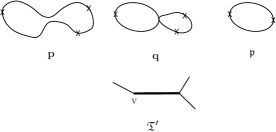
Figure 2. ${\bf p},{\bf q},{\mathfrak{p}}$

Convention 7.2.

We use specific letters/font in the notations of this paper.

1. ${\bf p,q}\in{\mathcal{M}}_{k+1,\ell}(X,L,J;\beta)$ for suitable $k,\ell,\beta$ depending on ${\bf p,q}$.

2. ${\bf x}\in{\mathcal{X}}_{k+1,\ell}(X,L;\beta)$, not necessarily pseudo-holomorphic, for suitable $k,\ell,\beta$ depending on ${\bf x}$.

3. $\mathfrak{p}\in{\mathfrak{P}}(k,\ell,\beta)$ for suitable $k,\ell,\beta$ depending on ${\mathfrak{p}}$. Here ${\mathfrak{P}}(k,\ell,\beta)$ is a finite subset of ${\mathcal{M}}_{k+1,\ell}(X,L,J;\beta)$. See, for example, (ob1) in Section 8.

The study of Situation 7.1 starts with Situation 7.7 in the next subsection after preparing and reviewing several notions.

For the actual construction, we need to specify how close ${\bf p}$ and ${\bf q}$ should be for an irreducible component of ${\bf q}$ to be a quasi-component of ${\bf p}$. We need to make such a choice inductively on $k+1,\ell$ and $\beta\cap[\omega]$.

To work out this induction process we need to consider also the following situation: “${\bf p}$ is close to ${\bf q}_{1}$ and ${\bf q}^{\prime}_{1}$ is an irreducible component of ${\bf q}_{1}$. ${\bf q}^{\prime}_{1}$ is close to ${\bf q}_{2}$ and ${\bf q}^{\prime}_{2}$ is an irreducible component of ${\bf q}_{2}$. ${\bf q}_{3}$ etc may appear in a similar way.” This iterated construction is carried out in Subsection 7.3.

7.2. Stabilization by interior marked points

The next definition is a variant of [FOOO8, Definition 9.7].

Definition 7.3.

Suppose we are in Situation 7.1. Type I stabilization data $(\vec{\mathfrak{w}}_{\mathfrak{p}},\vec{\mathcal{N}}_{\mathfrak{p}})$ at ${\mathfrak{p}}$ is the following data.

1. $\vec{\mathfrak{w}}_{\mathfrak{p}}=({\mathfrak{w}}_{{\mathfrak{p}},1},\dots,{\mathfrak{w}}_{{\mathfrak{p}},\ell^{\prime}})$ are distinct points in $\rm{Int}(\Sigma_{\mathfrak{p}})$ away from $\vec{\mathfrak{z}}_{\mathfrak{p}}$, the set of interior marked points of $\mathfrak{p}$. It is also away from nodal points.

2. $(\Sigma_{\mathfrak{p}},\vec{\mathfrak{w}}_{\mathfrak{p}})$ is stable, that is, the group

   $${\rm Aut}(\Sigma_{\mathfrak{p}},\vec{\mathfrak{w}}_{\mathfrak{p}})=\{v:\Sigma_{\mathfrak{p}}\to\Sigma_{\mathfrak{p}}:\text{biholomorphic},\,\,\,v({\mathfrak{w}}_{{\mathfrak{p}},i})={\mathfrak{w}}_{{\mathfrak{p}},i}\}$$

   is finite, except the case when the unique disk component of $\Sigma_{\mathfrak{p}}$ is unstable and the map $u_{\mathfrak{p}}$ is constant on it. In such a case the connected component of ${\rm Aut}(\Sigma_{\mathfrak{p}},\vec{\mathfrak{w}}_{\mathfrak{p}})$ is $S^{1}$ and $\pi_{0}{\rm Aut}(\Sigma_{\mathfrak{p}},\vec{\mathfrak{w}}_{\mathfrak{p}})$ is a finite group. See Figure 3. We explain this exceptional case more in Remark 7.4.

   

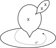
   Figure 3. Unstable element in $\mathcal{M}_{0,3}^{\rm d}$

3. $\vec{\mathcal{N}}_{\mathfrak{p}}=(\mathcal{N}_{{\mathfrak{p}},1},\dots,\mathcal{N}_{{\mathfrak{p}},\ell^{\prime}})$. Here $\mathcal{N}_{{\mathfrak{p}},i}$ is a codimension 2 submanifold of $X$.

4. There exists a neighborhood $U_{i}$ of $\mathfrak{w}_{{\mathfrak{p}},i}$ in $\Sigma_{\mathfrak{p}}$ such that $u_{\mathfrak{p}}(U_{i})$ intersects transversally with $\mathcal{N}_{{\mathfrak{p}},i}$ at the unique point $u_{\mathfrak{p}}(\mathfrak{w}_{{\mathfrak{p}},i})$. Moreover, the restriction of $u_{\mathfrak{p}}$ to $U_{i}$ is a smooth embedding. We require $\{U_{i}\}$ are disjoint.

5. Suppose that $v:\Sigma_{\mathfrak{p}}\to\Sigma_{\mathfrak{p}}$ is an extended automorphism of $\mathfrak{p}$. Then there exists a permutation $\sigma:\{1,\dots,\ell^{\prime}\}\to\{1,\dots,\ell^{\prime}\}$ such that $v({\mathfrak{w}}_{{\mathfrak{p}},i})={\mathfrak{w}}_{{\mathfrak{p}},\sigma(i)}$, $\mathcal{N}_{{\mathfrak{p}},i}=\mathcal{N}_{{\mathfrak{p}},\sigma(i)}$, and $v(U_{i})=U_{\sigma(i)}$.

We decompose $\Sigma_{\mathfrak{p}}$ as in (7.3). For each irreducible component $\Sigma_{\mathfrak{p}}^{\rm d}$, (resp. $\Sigma_{{\mathfrak{p}},\mathfrak{v}}^{\bf s}$) we put $\vec{\mathfrak{w}}_{\mathfrak{p}}\cap\Sigma_{{\mathfrak{p}}}^{{\rm d}}$, (resp. $\vec{\mathfrak{w}}_{\mathfrak{p}}\cap\Sigma_{{\mathfrak{p}},\mathfrak{v}}^{\bf s}$) together with (necessarily interior) nodes on it. We denote it by $(\Sigma_{{\mathfrak{p}}}^{{\rm d}},\vec{\mathfrak{w}}_{{\mathfrak{p}}}^{\rm d})$ (resp. $(\Sigma_{{\mathfrak{p}},\mathfrak{v}}^{\rm s},\vec{\mathfrak{w}}_{{\mathfrak{p}},\mathfrak{v}}^{\rm s})$). They are stable and so determine an element of $\mathcal{M}_{0,\ell_{\rm d}}^{\rm d}$ (resp. elements of $\mathcal{M}^{\rm s}_{\ell_{\mathfrak{v}}}$). Here $\mathcal{M}_{0,\ell_{\rm d}}^{\rm d}$ is the compactified moduli space of disks with $\ell_{\rm d}$ interior marked points and $\mathcal{M}^{\rm s}_{\ell_{\mathfrak{v}}}$ is the compactified moduli space of spheres with $\ell_{\mathfrak{v}}$ marked points. We denote by $\pi:\mathcal{C}^{\rm s}_{\ell}\to\mathcal{M}_{\ell}^{\rm s}$ the universal families of deformation.

Remark 7.4.

Here we consider the moduli space $\mathcal{M}_{0,\ell_{\rm d}}^{\rm d}$ of genus zero curves with one boundary component and without boundary marked points. If we define it in the same way as in Definition 2.2 assuming the stability in the sense of Definition 2.3, then such space is not compact. To compactify it we need to add isomorphism classes of elements $(\Sigma,\vec{\mathfrak{z}})$ such that $\Sigma$ has a disk component that has only one double point and that none of the marked points $\vec{\mathfrak{z}}$ are on this disk components. See Figure 3. The group of extended automorphisms of such an element $(\Sigma,\vec{\mathfrak{z}})$ contains $S^{1}$ consisting of rotations of the disk component. Therefore it is not stable in the sense of Definition 2.3. The moduli space of such objects is diffeomorphic to $\mathcal{M}_{\ell_{\rm d}+1}^{\rm s}$, the compactified moduli space of spheres with $\ell_{\rm d}+1$ marked points. We add the isomorphism classes of such objects to $\mathcal{M}_{0,\ell_{\rm d}}^{\rm d}$ and call the resulting moduli space a compactified moduli space of stable disks with $\ell_{\rm d}$ interior marked points by an abuse of notation. (Since the isotropy group $S^{1}$ is compact, this space is still Hausdorff.) This is an orbifold with boundary and corners. The object described in Figure 3, determines a boundary component of it. See [FOOO2, Subsection 7.4.1] for the discussion of this extra boundary component.

The universal family $\pi:\mathcal{C}_{0,\ell}^{\rm d}\to\mathcal{M}_{0,\ell}^{\rm d}$ is not well-defined on this boundary component for the part of disk component, because of the automorphism $S^{1}$. The universal family is defined outside of this disk component, which is in the fiber of the above mentioned component of the boudary.

The condition we required in Definition 7.3 (2) implies that $(\Sigma_{{\mathfrak{p}}}^{\rm d},\vec{\mathfrak{w}}_{{\mathfrak{p}}}^{\rm d})$ is in this extra boundary component only when $u_{\mathfrak{p}}$ is constant on the disk component.

The next definition is a variant of [FOOO8, Situation 9.8].

Definition 7.5.

Type I strong stabilization data at ${\mathfrak{p}}$ are type I stabilization data $(\vec{\mathfrak{w}}_{\mathfrak{p}},\vec{\mathcal{N}}_{\mathfrak{p}})$ together with the following data $((\vec{\mathcal{V}}_{\mathfrak{p}},\vec{\phi_{{\mathfrak{p}}}}),\vec{\varphi}_{\mathfrak{p}})$.

1. A neighborhood $\mathcal{V}_{{\mathfrak{p}}}^{{\rm d}}$ of $[(\Sigma_{{\mathfrak{p}}}^{{\rm d}},\vec{\mathfrak{w}}_{{\mathfrak{p}}}^{{\rm d}})]$ in $\mathcal{M}_{0,\ell_{\rm d}}^{\rm d}$ and neighborhoods $\mathcal{V}_{{\mathfrak{p}},\mathfrak{v}}^{\rm s}$ of $[(\Sigma_{{\mathfrak{p}},\mathfrak{v}}^{\rm s},\vec{\mathfrak{w}}_{{\mathfrak{p}},{\mathfrak{v}}}^{\rm s})]$ in $\mathcal{M}^{\rm s}_{\ell_{\mathfrak{v}}}$.

2. Diffeomorphisms $\phi_{{\mathfrak{p}}}^{{\rm d}}:\mathcal{V}_{{\mathfrak{p}}}^{{\rm d}}\times\Sigma_{{\mathfrak{p}}}^{{\rm d}}\to\pi^{-1}(\mathcal{V}_{{\mathfrak{p}}}^{{\rm d}})$, $\phi_{{\mathfrak{p}},\mathfrak{v}}^{\rm s}:\mathcal{V}_{{\mathfrak{p}},\mathfrak{v}}^{\rm s}\times\Sigma_{{\mathfrak{p}},\mathfrak{v}}^{\rm s}\to\pi^{-1}(\mathcal{V}_{{\mathfrak{p}},\mathfrak{v}}^{\rm s})$ which commute with projections.

3. Analytic families of coordinates $\vec{\varphi}_{\mathfrak{p}}$ at (interior) nodes which are compatible with the trivialization in (7) in the sense of [FOOO8, Definition 3.7].

4. Let $\mathfrak{s}_{i,{\mathfrak{p}}}^{{\rm d}}:\mathcal{V}_{{\mathfrak{p}}}^{{\rm d}}\to\mathcal{C}_{0,\ell_{\rm d}}^{\rm d}$, $\mathfrak{s}_{i,{\mathfrak{p}},{\mathfrak{v}}}^{\rm s}:\mathcal{V}_{{\mathfrak{p}},{\mathfrak{v}}}^{\rm s}\to\mathcal{C}_{\ell_{\mathfrak{v}}}^{\rm s}$ be the sections assigning the $i$-th marked point. (See [FOOO8, Section 2].) Then

   $$\mathfrak{s}_{i,{\mathfrak{p}}}^{{\rm d}}({\mathfrak{p}}^{\prime}) =\phi_{{\mathfrak{p}}}^{{\rm d}}({\mathfrak{p}}^{\prime},\mathfrak{s}_{i,{\mathfrak{p}}}^{{\rm d}}({\mathfrak{p}})),$$

   $$\mathfrak{s}_{i,{\mathfrak{p}},{\mathfrak{v}}}^{\rm s}({\mathfrak{p}}^{\prime}) =\phi_{{\mathfrak{p}},{\mathfrak{v}}}^{\rm s}({\mathfrak{p}}^{\prime},\mathfrak{s}_{i,{\mathfrak{p}},{\mathfrak{v}}}^{\rm s}({\mathfrak{p}})).$$

   In other words, the trivialization (7) respects the marked points.

5. The trivialization (7) is compatible with the action of extended automorphism group of $\mathfrak{p}$, which is induced by (5).

Definition 7.6.

Let type I strong stabilization data $((\vec{\mathfrak{w}}_{\mathfrak{p}},\vec{\mathcal{N}}_{\mathfrak{p}}),(\vec{\mathcal{V}_{\mathfrak{p}}},\vec{\phi_{\mathfrak{p}}}),\vec{\varphi}_{\mathfrak{p}})$ be chosen. Then an obstruction space $E_{\mathfrak{p}}$ at ${\mathfrak{p}}$ is defined to be a finite dimensional subspace of $C^{\infty}(\Sigma_{\mathfrak{p}},u_{\mathfrak{p}}^{*}TX\otimes\Lambda^{0,1})$ satisfying the following properties:

1. The union of the supports of the elements of $E_{\mathfrak{p}}$, which we denote by ${\rm Supp}(E_{\mathfrak{p}})$, is disjoint from the boundary, nodes, and marked points, but contains $\vec{\mathfrak{w}}_{\mathfrak{p}}$.

2. We consider the operator

   $$D_{u_{\mathfrak{p}}}\overline{\partial}:W^{2}_{m+1}((\Sigma_{\mathfrak{p}},\partial\Sigma_{\mathfrak{p}});u_{\mathfrak{p}}^{*}TX,u_{\mathfrak{p}}^{*}TL)\to L^{2}_{m}(\Sigma_{\mathfrak{p}},u_{\mathfrak{p}}^{*}TX\otimes\Lambda^{0,1})$$

   as in [FOOO8, (5.1)]. Then

   $${\rm Im}D_{u_{\mathfrak{p}}}\overline{\partial}+E_{\mathfrak{p}}=L^{2}_{m}(\Sigma_{\mathfrak{p}},u_{\mathfrak{p}}^{*}TX\otimes\Lambda^{0,1}).$$

3. Let

   $${\mathcal{EV}}:W^{2}_{m+1}((\Sigma_{\mathfrak{p}},\partial\Sigma_{\mathfrak{p}});u_{\mathfrak{p}}^{*}TX,u_{\mathfrak{p}}^{*}TL)\to T_{u_{\mathfrak{p}}(z_{0})}L$$

   be the linearized evaluation map at $z_{0}$. Then its restriction

   $${\mathcal{EV}}:(D_{u_{\mathfrak{p}}}\overline{\partial})^{-1}(E_{\mathfrak{p}})\to T_{u_{\mathfrak{p}}(z_{0})}L$$

   is surjective.

4. $E_{\mathfrak{p}}$ is invariant under the action of the extended automorphism group ${\rm Aut}^{+}({\mathfrak{p}})$.

5. The action of ${\rm Aut}({\mathfrak{p}})$ on $(D_{u_{\mathfrak{p}}}\overline{\partial})^{-1}(E_{\mathfrak{p}})/{\mathfrak{aut}}(\Sigma_{\mathfrak{p}},\vec{z}_{\mathfrak{p}},\vec{\mathfrak{z}}_{\mathfrak{p}})$ is effective.

6. If $u_{\mathfrak{p}}$ is constant on an irreducible component of $\Sigma_{\mathfrak{p}}$, then the support ${\rm Supp}(E_{\mathfrak{p}})$ is disjoint from this irreducible component.

We consider type I strong stabilization data $((\vec{\mathfrak{w}}_{\mathfrak{p}},\vec{\mathcal{N}}_{\mathfrak{p}}),(\vec{\mathcal{V}_{\mathfrak{p}}},\vec{\phi_{\mathfrak{p}}}),\vec{\varphi}_{\mathfrak{p}})$ together with an obstruction space $E_{\mathfrak{p}}$ and write

$$\Xi_{\mathfrak{p}}=((\vec{\mathfrak{w}}_{\mathfrak{p}},\vec{\mathcal{N}}_{\mathfrak{p}}),(\vec{\mathcal{V}_{\mathfrak{p}}},\vec{\phi_{\mathfrak{p}}}),\vec{\varphi}_{\mathfrak{p}},E_{\mathfrak{p}}).$$

Situation 7.7.

Suppose we are in Situation 7.1 and $\Xi_{\mathfrak{p}}$ is given. Let

$${\bf x}\in B_{\epsilon_{0}}({\mathcal{X}},{\bf p}).$$ (7.4)

Let $\epsilon_{2}$, $\epsilon_{1}$ be the constants given as in (7.1), (7.2) and $\epsilon_{0}$ be as in (7.4). For a positive number $\delta$ we will take positive constants $\epsilon_{2}(\delta,{\mathfrak{p}},\Xi_{\mathfrak{p}})$, $\epsilon_{1}(\delta,{\bf q},{\mathfrak{p}},\Xi_{\mathfrak{p}})$, $\epsilon_{0}(\delta,{\bf p},{\bf q},{\mathfrak{p}},\Xi_{\mathfrak{p}})$ which depend on the data in the parenthesis. We will assume

$$\epsilon_{2} <\epsilon_{2}(\delta,{\mathfrak{p}},\Xi_{\mathfrak{p}}),$$ (7.5)

$$\epsilon_{1} <\epsilon_{1}(\delta,{\bf q},{\mathfrak{p}},\Xi_{\mathfrak{p}}),$$

$$\epsilon_{0} <\epsilon_{0}(\delta,{\bf p},{\bf q},{\mathfrak{p}},\Xi_{\mathfrak{p}}).$$

We denote by $\Sigma_{{\bf q},{\rm v}}$ the source curve of the irreducible component ${\bf q}_{\rm v}$. Here ${\rm v}$ and ${\bf q}_{\rm v}$ are as in Situation 7.1. $\diamond$

Lemma 7.8.

For any sufficiently small $\delta>0$ there exist positive numbers $\epsilon_{2}(\delta,{\mathfrak{p}},\Xi_{\mathfrak{p}})$, $\epsilon_{1}(\delta,{\bf q},{\mathfrak{p}},\Xi_{\mathfrak{p}})$, $\epsilon_{0}(\delta,{\bf p},{\bf q},{\mathfrak{p}},\Xi_{\mathfrak{p}})$ with the following properties:

Suppose we are in Situation 7.7, especially we assume (7.5). Then there exists a unique collection of marked points

$$\vec{\mathfrak{w}}_{{\bf x};{\mathfrak{p}}},\quad\vec{\mathfrak{w}}_{{\bf p};{\mathfrak{p}}},\quad\vec{\mathfrak{w}}_{{\bf q};{\mathfrak{p}}}$$

such that

1. ${\mathfrak{w}}_{{\bf x};{\mathfrak{p}},i}\in\Sigma_{\bf x}$, ${\mathfrak{w}}_{{\bf p};{\mathfrak{p}},i}\in\Sigma_{\bf p}$, ${\mathfrak{w}}_{{\bf q};{\mathfrak{p}},i}\in\Sigma_{{\bf q},{\rm v}}$ for $i=1,\ldots,\ell^{\prime}$.

2. $u_{\bf x}({\mathfrak{w}}_{{\bf x};{\mathfrak{p}},i})\in\mathcal{N}_{{\mathfrak{p}},i}$, $u_{\bf p}({\mathfrak{w}}_{{\bf p};{\mathfrak{p}},i})\in\mathcal{N}_{{\mathfrak{p}},i}$, $u_{{\bf q}}({\mathfrak{w}}_{{\bf q};{\mathfrak{p}},i})\in\mathcal{N}_{{\mathfrak{p}},i}$.

3. $$d((\Sigma_{\mathfrak{p}},z_{\mathfrak{p}},\mathfrak{z}_{\mathfrak{p}}\cup\vec{\mathfrak{w}}_{\mathfrak{p}}),(\Sigma_{{\bf q},{\rm v}},z_{{\bf q},{\rm v}},\mathfrak{z}_{{\bf q},{\rm v}}\cup\vec{\mathfrak{w}}_{{\bf q};{\mathfrak{p}}})) <\delta,$$

   $$d((\Sigma_{{\bf q}},z_{{\bf q}},\mathfrak{z}_{{\bf q}}\cup\vec{\mathfrak{w}}_{{\bf q};{\mathfrak{p}}}),(\Sigma_{\bf p},z_{{\bf p}},\mathfrak{z}_{{\bf p}}\cup\vec{\mathfrak{w}}_{{\bf p};{\mathfrak{p}}})) <\delta,$$

   $$d((\Sigma_{{\bf p}},z_{{\bf p}},\mathfrak{z}_{{\bf p}}\cup\vec{\mathfrak{w}}_{{\bf p},{\mathfrak{p}}}),(\Sigma_{\bf x},z_{{\bf x}},\mathfrak{z}_{{\bf x}}\cup\vec{\mathfrak{w}}_{{\bf x},{\mathfrak{p}}})) <\delta.$$

   Here $d$’s are the metrics on various moduli spaces of marked stable curves. We fix such metrics. $z_{{\bf q},{\rm v}}$ (resp. $\mathfrak{z}_{{\bf q},{\rm v}}$) are boundary (resp. interior) marked or nodal points of ${\bf q}$ contained in $\Sigma_{{\bf q},{\rm v}}$.

Proof.

We first find $\vec{\mathfrak{w}}_{{\bf q};{\mathfrak{p}}}$ by the Implicit Function Theorem and the property ${\bf q}_{\rm v}\in B_{\epsilon_{2}}({\mathcal{X}},{\mathfrak{p}})$. (See [FOOO8, Lemma 9.9]). Then using $\vec{\mathfrak{w}}_{{\bf q};{\mathfrak{p}}}$ we can find $\vec{\mathfrak{w}}_{{\bf x};{\mathfrak{p}}}$, $\vec{\mathfrak{w}}_{{\bf p};{\mathfrak{p}}}$ by the Implicit Function Theorem and (7.1), (7.2) and (7.4). ∎

We consider the forgetful map

$$\mathfrak{forget}_{k+1,\ell+\ell^{\prime};0,\ell^{\prime}}:\mathcal{M}_{k+1,\ell+\ell^{\prime}}^{\rm d}\to\mathcal{M}_{0,\ell^{\prime}}^{\rm d}$$

which forgets all the boundary marked points and the first $\ell$ interior marked points. (Here $\ell^{\prime}$ is the cardinality of $\vec{\mathfrak{w}}_{\mathfrak{p}}$.)

Lemma 7.9.

Under the assumption of Lemma 7.8 we have

$$d((\Sigma_{\mathfrak{p}},\vec{\mathfrak{w}}_{\mathfrak{p}}),\mathfrak{forget}_{k_{\rm d}+1,\ell_{\rm d};0,\ell^{\prime}}(\Sigma_{{\bf q},{\rm v}},z_{{\bf q},{\rm v}},\vec{\mathfrak{w}}_{{\bf q};{\mathfrak{p}}})) <\delta,$$

$$d((\Sigma_{\mathfrak{p}},\vec{\mathfrak{w}}_{\mathfrak{p}}),\mathfrak{forget}_{k+1,\ell+\ell^{\prime};0,\ell^{\prime}}(\Sigma_{{\bf q}},z_{{\bf q}},\mathfrak{z}_{{\bf q}}\cup\vec{\mathfrak{w}}_{{\bf q},{\mathfrak{p}}})) <\delta,$$

$$d((\Sigma_{\mathfrak{p}},\vec{\mathfrak{w}}_{\mathfrak{p}}),\mathfrak{forget}_{k+1,\ell+\ell^{\prime};0,\ell^{\prime}}(\Sigma_{{\bf p}},z_{{\bf p}},\mathfrak{z}_{{\bf p}}\cup\vec{\mathfrak{w}}_{{\bf p},{\mathfrak{p}}})) <\delta,$$

$$d((\Sigma_{\mathfrak{p}},\vec{\mathfrak{w}}_{\mathfrak{p}}),\mathfrak{forget}_{k+1,\ell+\ell^{\prime};0,\ell^{\prime}}(\Sigma_{{\bf x}},z_{{\bf x}},\mathfrak{z}_{{\bf x}}\cup\vec{\mathfrak{w}}_{{\bf x},{\mathfrak{p}}})) <\delta.$$

Figure 4. Forgetting marked points $\vec{z}$, $\vec{\mathfrak{z}}$

Proof.

The first inequality is a consequence of Lemma 7.8 (3) and the continuity of the forgetful map. The second inequality is a consequence of the first inequality and the equality

$$\mathfrak{forget}_{k+1,\ell+\ell^{\prime};0,\ell^{\prime}}(\Sigma_{{\bf q}},z_{{\bf q}},\mathfrak{z}_{{\bf q}}\cup\vec{\mathfrak{w}}_{{\bf q},{{\mathfrak{p}}}})=(\Sigma_{{\bf q},{\rm v}},\vec{\mathfrak{w}}_{{\bf q};{\mathfrak{p}}}).$$

See Figure 4. We remark that this is the place where we use the fact we are studying bordered Riemann surfaces of genus 0.

The third and fourth inequalities then follow from the continuity of $\mathfrak{forget}_{k+1,\ell+\ell^{\prime};0,\ell^{\prime}}$. ∎

We use the data given in Definition 7.5 (7), (8) to define a smooth open embedding $\Phi$ below:

$$\Phi:\mathcal{V}_{{\mathfrak{p}}}^{{\rm d}}\times\prod_{\mathfrak{v}}\mathcal{V}_{{\mathfrak{p}},{\mathfrak{v}}}^{\rm s}\times(D^{2}(c))^{m_{\rm s}}\to\mathcal{M}_{0,\ell^{\prime}}^{\rm d}$$ (7.6)

as in [FOOO8, (3.5)]. The first and second factors parametrize the deformation of each irreducible component and the third factor is the gluing parameter, where $m_{\rm s}$ is the number of interior nodes of $\Sigma_{\mathfrak{p}}$.

By Lemma 7.9 there exist elements $\mathfrak{x}\in\mathcal{V}_{{\mathfrak{p}}}^{{\rm d}}\times\prod_{\mathfrak{v}}\mathcal{V}_{{\mathfrak{p}},{\mathfrak{v}}}^{\rm s}$ and $\vec{\epsilon}\in(D^{2}(c))^{m_{\rm s}}$ such that

$$\mathfrak{forget}_{k+1,\ell+\ell^{\prime};0,\ell^{\prime}}(\Sigma_{{\bf x}},z_{{\bf x}},\mathfrak{z}_{{\bf x}}\cup\vec{\mathfrak{w}}_{{\bf x},{\mathfrak{p}}})=\Phi(\mathfrak{x};\vec{\epsilon}).$$

Let $\Sigma_{{\mathfrak{p}}}(\epsilon)$ be the $\epsilon$-thick part of $\Sigma_{{\mathfrak{p}}}$. Using the data given in Definition 7.5 (7), (8), we can apply [FOOO8, Lemma 3.9] to obtain

$$\widehat{\Phi}_{\mathfrak{r},\vec{\epsilon}}:\mathcal{V}\times\Sigma_{{\mathfrak{p}}}(\epsilon)\to\mathcal{C}^{\rm d}_{0,\ell}$$

and smooth embeddings,

$$\widehat{\Phi}_{{\bf q},{\mathfrak{p}};\Xi_{\mathfrak{p}}} :{\rm Supp}(E_{\mathfrak{p}})\to\Sigma_{{\bf q}},$$ (7.7)

$$\widehat{\Phi}_{{\bf p},{\mathfrak{p}};\Xi_{\mathfrak{p}}} :{\rm Supp}(E_{\mathfrak{p}})\to\Sigma_{{\bf p}},$$

$$\widehat{\Phi}_{{\bf x},{\mathfrak{p}};\Xi_{\mathfrak{p}}} :{\rm Supp}(E_{\mathfrak{p}})\to\Sigma_{{\bf x}}.$$

For example, the third map is a restriction of the map $\widehat{\Phi}_{\mathfrak{x};\vec{\epsilon}}$ appearing in [FOOO8, Lemma 3.9].

Remark 7.10.

In the case where $(\Sigma_{\mathfrak{p}},\vec{\mathfrak{w}}_{\mathfrak{p}})$ is the point appearing in Remark 7.4 and Figure 3, the map (7.6) becomes

$$\Phi:\prod_{\mathfrak{v}}\mathcal{V}_{{\mathfrak{p}},{\mathfrak{v}}}^{\rm s}\times[0,c)\times(D^{2}(c))^{m_{\rm s}-1}\to\mathcal{M}_{0,\ell^{\prime}}^{\rm d}.$$ (7.8)

Here $[0,c)$ is the space of smoothing parameters of the node which lies on the disk component. (See [FOOO2, pages 590-591].) By Definition 7.6 (6), ${\rm Supp}(E_{\mathfrak{p}})$, the support of the obstruction bundle, is disjoint from the disk component. (This is because $u_{\mathfrak{p}}$ is constant on the disk component as we explained in Remark 7.4.) We use this fact to show that (7.7) is also defined in this case.

Lemma 7.11.

We can choose $\epsilon_{2}(\delta,{\mathfrak{p}},\Xi_{\mathfrak{p}})$, $\epsilon_{1}(\delta,{\bf q},{\mathfrak{p}},\Xi_{\mathfrak{p}})$, $\epsilon_{0}(\delta,{\bf p},{\bf q},{\mathfrak{p}},\Xi_{\mathfrak{p}})$ so that, under the assumption of Lemma 7.8 the maps (7.7) have the following properties:

1. Denote by $d_{C^{2},{\rm Supp}(E_{\mathfrak{p}})}$ the $C^{2}$ distance between two maps: ${\rm Supp}(E_{\mathfrak{p}})\to X$. Then the following inequalities hold:

   $$d_{C^{2},{\rm Supp}(E_{\mathfrak{p}})}\left(u_{{\bf q}}\circ\widehat{\Phi}_{{\bf q},{\mathfrak{p}};\Xi_{\mathfrak{p}}},u_{{\mathfrak{p}}}\right)<\delta,$$ (7.9)

   $$d_{C^{2},{\rm Supp}(E_{\mathfrak{p}})}\left(u_{{\bf p}}\circ\widehat{\Phi}_{{\bf p},{\mathfrak{p}};\Xi_{\mathfrak{p}}},u_{\mathfrak{p}}\right)<\delta,$$

   $$d_{C^{2},{\rm Supp}(E_{\mathfrak{p}})}\left(u_{{\bf x}}\circ\widehat{\Phi}_{{\bf x},{\mathfrak{p}};\Xi_{\mathfrak{p}}},u_{\mathfrak{p}}\right)<\delta.$$

2. The next inequalities hold for each $x\in{\rm Supp}(E_{\mathfrak{p}})$:

   $$|\partial\,\widehat{\Phi}_{{\bf q},{\mathfrak{p}};\Xi_{\mathfrak{p}}}(x)| >10|\overline{\partial}\,\widehat{\Phi}_{{\bf q},{\mathfrak{p}};\Xi_{\mathfrak{p}}}(x)|,$$ (7.10)

   $$|\partial\,\widehat{\Phi}_{{\bf p},{\mathfrak{p}};\Xi_{\mathfrak{p}}}(x)| >10|\overline{\partial}\,\widehat{\Phi}_{{\bf p},{\mathfrak{p}};\Xi_{\mathfrak{p}}}(x)|,$$

   $$|\partial\,\widehat{\Phi}_{{\bf x},{\mathfrak{p}};\Xi_{\mathfrak{p}}}(x)| >10|\overline{\partial}\,\widehat{\Phi}_{{\bf x},{\mathfrak{p}};\Xi_{\mathfrak{p}}}(x)|.$$

Proof.

The inequalities (7.10) are easy consequences of the definition of $\widehat{\Phi}_{*,\mathfrak{p},\Xi_{\mathfrak{p}}}$ in (7.7) and Lemma 7.9. The inequalities (7.9) are consequences of Lemma 7.9, and the fact that ${\rm Supp}(E_{\mathfrak{p}})$ is away from the node. The proof of (7.9) is the same as that of [FOOO3, Lemma 4.3.75]. We repeat the proof for completeness’ sake. We prove the second inequality only. The proofs of other two inequalities are similar. Lemma 7.9 implies that $(\Sigma_{\bf p},\vec{\mathfrak{w}}_{{\bf p},\mathfrak{p}})\in B_{\epsilon}((\Sigma_{\bf q},\vec{\mathfrak{w}}_{{\bf q},\mathfrak{p}}))$ for some $\epsilon$ going to zero as $\epsilon_{1},\epsilon_{2}$ go to zero, where we fix and use a metric on the compactified moduli space ${\mathcal{M}}_{0,\ell_{\mathfrak{p}}}^{\rm d}$ of disks with $\ell_{\mathfrak{p}}$ interior marked points to define $B_{\epsilon}((\Sigma_{\bf q},\vec{\mathfrak{w}}_{{\bf q},\mathfrak{p}}))$. (Here $\ell_{\mathfrak{p}}$ is the cardinality of the set $\vec{\mathfrak{w}}_{\mathfrak{p}}$.) We take an analytic family of coordinates at nodal points which has the following properties.

Definition 7.12.

1. A holomorphic embedding $D^{2}\to S^{2}$ is said to be extendable if it is a restriction of a biholomorphic map $S^{2}\to S^{2}$.

2. A holomorphic embedding $D^{2}\to D^{2}$ is said to be extendable if it is a restriction of biholomorphic map $D^{2}(R)\to D^{2}$ for some $R>1$.

3. A holomorphic embedding $(D_{\geq 0}^{2},\partial D_{\geq 0}^{2})\to(D^{2},\partial D^{2})$ is said to be extendable if its double is extendable in the sense of $(1)$. Here $D_{\geq 0}^{2}=\{z\in D^{2}~{}|~{}{\rm Im}\,z\geq 0\}$.

4. An analytic family of coordinates is said to be extendable if its members are extendable in the sense of (1),(2) or (3).

Note that $d({\bf q}_{\rm v},\mathfrak{p})$ is assumed to be small. So there exists an embedding

$$\widehat{\Phi}_{{\bf q}_{\rm v},{\mathfrak{p}};\Xi_{\mathfrak{p}}}:{\rm Supp}(E_{\mathfrak{p}})\to\Sigma_{{\bf q}_{\rm v}}$$

such that

$$d_{C^{2},{\rm Supp}(E_{\mathfrak{p}})}\left(u_{{\bf q}}\circ\widehat{\Phi}_{{\bf q}_{\rm v},{\mathfrak{p}};\Xi_{\mathfrak{p}}},u_{{\mathfrak{p}}}\right)<\delta/10.$$ (7.11)

(Actually $\widehat{\Phi}_{{\bf q}_{\rm v},{\mathfrak{p}};\Xi_{\mathfrak{p}}}=\widehat{\Phi}_{{\bf q},{\mathfrak{p}};\Xi_{\mathfrak{p}}}$.) Using $(\Sigma_{\bf p},\vec{\mathfrak{w}}_{{\bf p},\mathfrak{p}})\in B_{\epsilon}((\Sigma_{\bf q},\vec{\mathfrak{w}}_{{\bf q},\mathfrak{p}}))$ and data (7)(8) of Definition 7.5, $\Xi_{(\Sigma_{\bf q},\vec{\mathfrak{w}}_{{\bf q},\mathfrak{p}})}$, at $(\Sigma_{\bf q},\vec{\mathfrak{w}}_{{\bf q},\mathfrak{p}})$, we obtain an embedding

$$\widehat{\Phi}_{{\bf p},{\bf q};\Xi_{(\Sigma_{\bf q},\vec{\mathfrak{w}}_{{\bf q},\mathfrak{p}})}}:\Sigma_{\bf q}\setminus\text{(neck region)}\to\Sigma_{\bf p}$$

such that

$$d_{C^{2},\widehat{\Phi}_{{\bf q}_{\rm v},{\mathfrak{p}};\Xi_{\mathfrak{p}}}({\rm Supp}(E_{\mathfrak{p}}))}\left(u_{{\bf p}}\circ\widehat{\Phi}_{{\bf p},{\bf q};\Xi_{(\Sigma_{\bf q},\vec{\mathfrak{w}}_{{\bf q},\mathfrak{p}})}},u_{{\bf q}}\right)<\delta/10,$$ (7.12)

where $\widehat{\Phi}_{{\bf p},{\bf q};\Xi_{(\Sigma_{\bf q},\vec{\mathfrak{w}}_{{\bf q},\mathfrak{p}})}}$ is a map defined in the way similar to (7.7) using the data $\Xi_{(\Sigma_{\bf q},\vec{\mathfrak{w}}_{{\bf q},\mathfrak{p}})}$. We put

$$(\Sigma_{\bf p},\vec{\mathfrak{w}}_{{\bf p},\mathfrak{p}})=\Phi(\vec{\mathfrak{x}},\vec{\rho}),$$

where $\vec{\mathfrak{x}}$ is the parameter to deform the complex structure of the irreducible components of ${\bf q}$ and $\vec{\rho}$ is a smoothing parameter of the nodes of ${\bf q}$. We use $\Xi_{(\Sigma_{\bf q},\vec{\mathfrak{w}}_{{\bf q},\mathfrak{p}})}$ to define the map $\Phi$ in a way similar to (7.6).

We take $\vec{\mathfrak{x}}_{0}$ such that $\Phi(\vec{\mathfrak{x}}_{0},\vec{0})=(\Sigma_{\bf q},\vec{\mathfrak{w}}_{{\bf q},{\mathfrak{p}}})$. (Namely $\vec{\mathfrak{x}}_{0}$ corresponds to the complex structure of $\Sigma_{\bf q}$ itself.)

Sublemma 7.13.

If $(\Sigma_{\bf p},\vec{\mathfrak{w}}_{{\bf p},{\mathfrak{p}}})=\Phi(\vec{\mathfrak{x}}_{0},\vec{\rho})$ for some $\vec{\rho}$ and if the analytic families of coordinates, which are part of the data $\Xi_{(\Sigma_{\bf q},\vec{\mathfrak{w}}_{{\bf q},\mathfrak{p}})}$, are extendable, then

$$\widehat{\Phi}_{{\bf p},{\bf q};\Xi_{(\Sigma_{\bf q},\vec{\mathfrak{w}}_{{\bf q},\mathfrak{p}})}}\circ\widehat{\Phi}_{{\bf q}_{\rm v},{\mathfrak{p}};\Xi_{\mathfrak{p}}}=\widehat{\Phi}_{{\bf p},{\mathfrak{p}};\Xi_{\mathfrak{p}}}$$

on ${\rm Supp}(E_{\mathfrak{p}})$.

Proof.

There exists a biholomorphic map ${\mathfrak{I}}:(\Sigma_{\bf p},\vec{\mathfrak{w}}_{{\bf p},{\mathfrak{p}}})\to(\Sigma_{{\bf q}_{\rm v}},\vec{\mathfrak{w}}_{{\bf q},{\mathfrak{p}}})$ such that ${\mathfrak{I}}\circ\widehat{\Phi}_{{\bf p},{\bf q};\Xi_{(\Sigma_{\bf q},\vec{\mathfrak{w}}_{{\bf q},\mathfrak{p}})}}$ is the identity map on $\Sigma_{{\bf q}_{\rm v}}$ minus a small neighborhood of boundary nodes, if all the components of $\vec{\rho}$ are nonzero. (If some components are zero the domain is smaller but still contains the image of $\widehat{\Phi}_{{\bf p},{\mathfrak{p}};\Xi_{\mathfrak{p}}}$.) This is a consequence of the extendability of the analytic family of coordinates there. (See Figure 5 and also [Fu, Lemma 12.33].) The sublemma is an easy consequence of this fact. ∎

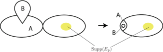
Figure 5. Sublemma 7.13

In the case of $(\Sigma_{\bf p},\vec{\mathfrak{w}}_{{\bf p},{\mathfrak{p}}})=\Phi(\vec{\mathfrak{x}}_{0},\vec{\rho})$ the second inequality of (7.9) follows from (7.11), (7.12) and Sublemma 7.13. The general case follows by taking $\epsilon_{1}$ (which estimates $d({\bf p},{\bf q})$ and hence $d(\vec{\mathfrak{x}},\vec{\mathfrak{x}}_{0})$) sufficiently small compared to the distance between ${\rm Supp}(E_{\mathfrak{p}})$ and nodes. ∎

Using Lemma 7.11 we construct a map

$$\mathcal{P}_{{\bf x},{\bf p},{\bf q},{\mathfrak{p}};\Xi_{\mathfrak{p}}}: C^{2}(\widehat{\Phi}_{{\bf x},{\mathfrak{p}};\Xi_{\mathfrak{p}}}(U({\rm Supp}(E_{\mathfrak{p}})));u_{\bf x}^{*}TX\otimes\Lambda^{0,1})$$ (7.13)

$$\to C^{2}(U({\rm Supp}(E_{\mathfrak{p}}));u_{\mathfrak{p}}^{*}TX\otimes\Lambda^{0,1})$$

as follows. (Here $U({\rm Supp}(E_{\mathfrak{p}}))$ is a sufficiently small open neighborhood of ${\rm Supp}(E_{\mathfrak{p}})$.) The map (7.13) is similar to the map [FOOO8, (8.1)].

Let $z\in U({\rm Supp}(E_{\mathfrak{p}}))$. By (7.9) $d(u_{\mathfrak{p}}(z),u_{\bf x}(\hat{\Phi}_{{\bf x},{\mathfrak{p}};\Xi_{\mathfrak{p}}}(z)))$ is smaller than the injectivity radius of $X$. So there exists a unique minimal geodesic joining them. We fix a unitary connection of $TX$. Using the parallel transport along the minimal geodesic we obtain $T_{\hat{\Phi}_{{\bf x},{\mathfrak{p}};\Xi_{\mathfrak{p}}}(z)}X\to T_{u_{\mathfrak{p}}(z)}X$. We thus obtain a bundle map

$$u_{\bf x}^{*}TX\to u_{\mathfrak{p}}^{*}TX$$ (7.14)

over $\hat{\Phi}_{{\bf x},{\mathfrak{p}};\Xi_{\mathfrak{p}}}^{-1}$.

On the other hand, the complex linear part of the differential of $\hat{\Phi}_{{\bf x},{\mathfrak{p}}}^{-1}$ induces a bundle map

$$\Lambda^{0,1}(\Sigma_{\bf x})\to\Lambda^{0,1}(\Sigma_{\mathfrak{p}})$$ (7.15)

over $\hat{\Phi}_{{\bf x},{\mathfrak{p}};\Xi_{\mathfrak{p}}}^{-1}$. ((7.10) implies that this map is a bundle isomorphism on $U({\rm Supp}(E_{\mathfrak{p}}))$.) The bundle map which is a tensor product (over ${\mathbb{C}}$) of (7.14) and (7.15) induces the map (7.13), which is an isomorphism.

We also consider ${\mathcal{P}}_{\mathbf{p},\mathbf{p},\mathbf{q},\mathfrak{p};\Xi_{\mathfrak{p}}}$ and ${\mathcal{P}}_{\mathbf{q},\mathbf{q},\mathbf{q},\mathfrak{p};\Xi_{\mathfrak{p}}}$.

We define:

$$E_{{\bf p},{\bf q},{\mathfrak{p}};\Xi_{\mathfrak{p}}}({\bf x})=(\mathcal{P}_{{\bf x},{\bf p},{\bf q},{\mathfrak{p}};\Xi_{\mathfrak{p}}})^{-1}(E_{\mathfrak{p}}).$$ (7.16)

Lemma 7.14.

${\bf x}\mapsto E_{{\bf p},{\bf q},{\mathfrak{p}};\Xi_{\mathfrak{p}}}({\bf x})$ is smooth in the sense of [FOOO8, Definition 8.7].

Proof.

The proof is the same as the one given in [FOOO8, Subsection 11.2] and so is omitted. ∎

7.3. Iteration of the construction of Subsection 7.2

The obstruction bundle data, which we will construct for the proof of Theorem 5.4, is obtained by taking an appropriate direct sum of the ones defined as in (7.16). More precisely we also need its variant which includes the iteration of the process appearing in Situation 7.1. In this subsection we will explain this variant. In the case $n=1$, Situation 7.15 becomes Situation 7.1.

Let $\mathfrak{T}\in\mathcal{G}(k+1,\ell,\beta)$. Let $\mathfrak{T}^{\prime}>\mathfrak{T}$, ${\rm v}$ an interior vertex of $\mathfrak{T}^{\prime}$, and let $\pi:\mathcal{T}\to\mathcal{T}^{\prime}$ be the projection canonically defined by a sequence of edge contraction. We say $\mathfrak{S}$ is a subtree of $\mathfrak{T}$ if it is obtained from $\pi^{-1}({\rm v})$ with data induced by $\mathfrak{T}$. A subtree $\mathfrak{S}$ is an element of some $\mathcal{G}(k^{\prime}+1,\ell^{\prime},\beta^{\prime})$. If ${\bf p}\in\mathcal{M}^{\circ}_{k+1,\ell}(X,L,J;\beta)(\mathfrak{T})$ and $\mathfrak{S}$ is a subtree of $\mathfrak{T}$, we obtain ${\bf p}_{\mathfrak{S}}\in\mathcal{M}_{k^{\prime}+1,\ell^{\prime}}(X,L,J;\beta^{\prime})$ by gluing ${\bf p}_{\rm v}$ for vertices ${\rm v}$ of $\mathfrak{S}$ in the way described by $\mathfrak{S}$. See Lemma 4.2 and its proof.

Situation 7.15.

Consider the data ${\bf p}$, ${\bf q}_{j}$, ${\mathfrak{p}}$, $\mathfrak{T}_{j}$, $\mathfrak{S}_{j}$, $\epsilon_{1,j}>0$ ($j=1,\dots,n$ for some $n=0,1,2,\dots$) and $\epsilon_{2}>0$ with the following properties. (See Figure 6.)

1. ${\bf p}\in\mathcal{M}_{k+1,\ell}(X,L,J;\beta)$.

2. ${\bf q}_{j}\in\mathcal{M}^{\circ}_{k_{j}+1,\ell_{j}}(X,L,J;\beta_{j})(\mathfrak{T}_{j})$. Here $\mathfrak{T}_{j}\in\mathcal{G}(k_{j}+1,\ell_{j},\beta_{j})$.

3. $d({\bf p},{\bf q}_{1})<\epsilon_{1,1}$. ($(k,\ell,\beta)=(k_{1},\ell_{1},\beta_{1})$ in particular.)

4. $\mathfrak{S}_{j}$ is a subtree of $\mathfrak{T}_{j}$. We define ${\bf q}_{j,\mathfrak{S}_{j}}$ as above. We assume ${\bf q}_{j,\mathfrak{S}_{j}}\neq{\bf q}_{j}$ for $j=1,\dots,n-1$.

5. For $j\leq n-1$ we require ${\bf q}_{j,\mathfrak{S}_{j}}\in\mathcal{M}_{k_{j+1}+1,\ell_{j+1}}(X,L,J;\beta_{j+1})$ and

   $$d({\bf q}_{j,\mathfrak{S}_{j}},{\bf q}_{j+1})<\epsilon_{1,j+1}.$$ (7.17)

6. We require ${\mathfrak{p}},{\bf q}_{n,\mathfrak{S}_{n}}\in\mathcal{M}^{\circ}_{k_{n+1}+1,\ell_{n+1}}(X,L,J;\beta_{n+1})$ and

   $$d({\bf q}_{n,\mathfrak{S}_{n}},{\mathfrak{p}})<\epsilon_{2}.$$ (7.18)

   (Note that $\mathfrak{S}_{n}$ has only one interior vertex by this condition.)

7. We require $\mathfrak{S}_{j}>\mathfrak{T}_{j+1}$. $\diamond$

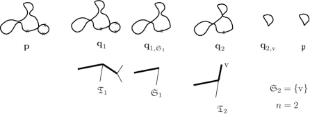
Figure 6. Situation 7.15

We take type I strong stabilization data and an obstruction space at $\mathfrak{p}$, which we denote by $\Xi_{\mathfrak{p}}$. (See Definition 7.5.) Let

$${\bf x}\in B_{\epsilon_{0}}({\mathcal{X}},{\bf p}).$$ (7.19)

Let $\delta_{j}$, $j=0,\dots,n+1$ be positive numbers. In the sequel we will find positive numbers:

$$\epsilon_{0}(\delta_{0};{\bf p},{\bf q}_{1},\dots,{\bf q}_{n},{\mathfrak{p}},\Xi_{\mathfrak{p}}),$$ (7.20)

$$\epsilon_{1,j}(\delta_{j};{\bf q}_{j},\dots,{\bf q}_{n},{\mathfrak{p}},\Xi_{\mathfrak{p}}),(j=1,2,\dots,n)$$

$$\epsilon_{2}(\delta_{n+1};{\mathfrak{p}},\Xi_{\mathfrak{p}}),$$

which depend on the data in the parenthesis and assume

$$\epsilon_{0} <\epsilon_{0}(\delta_{0};{\bf p},{\bf q}_{1},\dots,{\bf q}_{n},{\mathfrak{p}},\Xi_{\mathfrak{p}}),$$ (7.21)

$$\epsilon_{1,j} <\epsilon_{1,j}(\delta_{j};{\bf q}_{j},\dots,{\bf q}_{n},{\mathfrak{p}},\Xi_{\mathfrak{p}}),$$

$$\epsilon_{2} <\epsilon_{2}(\delta_{n+1};{\mathfrak{p}},\Xi_{\mathfrak{p}}).$$

Lemma 7.16.

There exist positive numbers as in (7.20) with the following properties: Suppose we are in Situation 7.15 (1)-(7), (7.19) and (7.21). Then there exists a collection of marked points

$$\vec{\mathfrak{w}}_{{\bf x};\mathfrak{p}},\quad\vec{\mathfrak{w}}_{{\bf p};{\mathfrak{p}}},\quad\vec{\mathfrak{w}}_{{\bf q}_{j},{\mathfrak{p}}}\enskip(j=1,\dots,n),$$

such that

1. ${\mathfrak{w}}_{{\bf x};{\mathfrak{p}},i}\in\Sigma_{\bf x}$, ${\mathfrak{w}}_{{\bf p};{\mathfrak{p}},i}\in\Sigma_{\bf p}$ and ${\mathfrak{w}}_{{\bf q}_{j};{\mathfrak{p}},i}\in\Sigma_{{\bf q}_{j,\mathfrak{S}_{j}}}$.

2. $u_{\bf x}({\mathfrak{w}}_{{\bf x};{\mathfrak{p}},i})\in\mathcal{N}_{{\mathfrak{p}},i}$, $u_{\bf p}({\mathfrak{w}}_{{\bf p};{\mathfrak{p}},i})\in\mathcal{N}_{{\mathfrak{p}},i}$ and $u_{{\bf q}_{j}}({\mathfrak{w}}_{{\bf q}_{j};{\mathfrak{p}},i})\in\mathcal{N}_{{\mathfrak{p}},i}$.

3. $$d((\Sigma_{{\bf q}_{j+1}},\vec{z}_{{\bf q}_{j+1}},\vec{\mathfrak{z}}_{{\bf q}_{j+1}}\cup\vec{\mathfrak{w}}_{{\bf q}_{j+1},{\mathfrak{p}}}),(\Sigma_{{\bf q}_{j,\mathfrak{S}_{j}}},\vec{z}_{{\bf q}_{j,\mathfrak{S}_{j}}},\vec{\mathfrak{z}}_{{\bf q}_{j,\mathfrak{S}_{j}}}\cup\vec{\mathfrak{w}}_{{\bf q}_{j},{\mathfrak{p}}})) <\delta_{j+1},$$

   $$d((\Sigma_{{\bf q}_{1}},\vec{z}_{{\bf q}_{1}},\vec{\mathfrak{z}}_{{\bf q}_{1}}\cup\vec{\mathfrak{w}}_{{\bf q}_{1};{\mathfrak{p}}}),(\Sigma_{\bf p},\vec{z}_{{\bf p}},\vec{\mathfrak{z}}_{{\bf p}}\cup\vec{\mathfrak{w}}_{{\bf p};{\mathfrak{p}}}) <\delta_{1},$$

   $$d((\Sigma_{{\bf p}},\vec{z}_{{\bf p}},\vec{\mathfrak{z}}_{{\bf p}}\cup\vec{\mathfrak{w}}_{{\bf p},{\mathfrak{p}}}),(\Sigma_{\bf x},\vec{z}_{{\bf x}},\vec{\mathfrak{z}}_{{\bf x}}\cup\vec{\mathfrak{w}}_{{\bf x},{\mathfrak{p}}})) <\delta_{0},$$

   $$d((\Sigma_{{\bf q}_{n},{\mathfrak{S}_{n}}},\vec{z}_{{\bf q}_{n},{\mathfrak{S}_{n}}},\vec{\mathfrak{z}}_{{\bf q}_{n},{\mathfrak{S}_{n}}}\cup\vec{\mathfrak{w}}_{{\bf q}_{n},{\mathfrak{p}}}),(\Sigma_{\mathfrak{p}},\vec{z}_{\mathfrak{p}},\vec{\mathfrak{z}}_{\mathfrak{p}}\cup\vec{\mathfrak{w}}_{{\mathfrak{p}}})) <\delta_{n+1}.$$

   Here $d$’s are the metrics on various moduli spaces of marked stable curves which we fix. $\vec{z}_{{\bf q}_{j,\mathfrak{S}_{j}}}$ (resp. $\vec{\mathfrak{z}}_{{\bf q}_{j,\mathfrak{S}_{j}}}$) are boundary (resp. interior) marked or nodal points of ${\bf q}_{j}$ contained in $\Sigma_{{\bf q}_{j,\mathfrak{S}_{j}}}$.

   When $n=0$ we have

   $$d((\Sigma_{\bf p},\vec{z}_{\bf p},\vec{\mathfrak{z}}_{\bf p}\cup\vec{\mathfrak{w}}_{{\bf p};\mathfrak{p}}),(\Sigma_{\mathfrak{p}},\vec{z}_{\mathfrak{p}},\vec{\mathfrak{z}}_{\mathfrak{p}}\cup\vec{\mathfrak{w}}_{\mathfrak{p}}))<\delta_{1},$$

   instead.

Proof.

Using the Implicit Function Theorem and the assumptions, we can find $\vec{\mathfrak{w}}_{{\bf q}_{j},{\mathfrak{p}}}$ ($j=1,\dots,n$) which have the required properties, by a downward induction on $j$. Then we can find $\vec{\mathfrak{w}}_{{\bf x};{\mathfrak{p}}}$, $\vec{\mathfrak{w}}_{{\bf p};{\mathfrak{p}}}$ in the same way as the proof of Lemma 7.8. ∎

Let $\delta^{\prime}_{j}$ be a sequence of positive numbers for $j=0,\dots,n+1$.

Lemma 7.17.

We can take $\delta_{j}=\delta(\delta^{\prime}_{j},{\bf q}_{j})$ (for $j\neq 0,n+1$), $\delta_{0}=\delta(\delta^{\prime}_{0},\bf p)$, $\delta_{n+1}=\delta(\delta^{\prime}_{n+1},\mathfrak{p})$ with the following properties. Under the assumption of Lemma 7.16 we have:

$$d((\Sigma_{\mathfrak{p}},\vec{\mathfrak{w}}_{\mathfrak{p}}),\mathfrak{forget}_{k^{1}_{j+1}+1,\ell^{1}_{j+1}+\ell^{\prime};0,\ell^{\prime}}(\Sigma_{{\bf q}_{j,\mathfrak{S}_{j}}},\vec{z}_{{\bf q}_{j,\mathfrak{S}_{j}}},\vec{\mathfrak{z}}_{{\bf q}_{j,\mathfrak{S}_{j}}}\cup\vec{\mathfrak{w}}_{{\bf q};{\mathfrak{p}}})) <\delta^{\prime}_{j+1}+\dots+\delta^{\prime}_{n+1},$$ (7.22)

$$d((\Sigma_{\mathfrak{p}},\vec{\mathfrak{w}}_{\mathfrak{p}}),\mathfrak{forget}_{k^{1}_{j}+1,\ell^{1}_{j}+\ell^{\prime};0,\ell^{\prime}}(\Sigma_{{\bf q}_{j}},\vec{z}_{{\bf q}_{j}},\vec{\mathfrak{z}}_{{\bf q}_{j}}\cup\vec{\mathfrak{w}}_{{\bf q}_{j},{\mathfrak{p}}})) <\delta^{\prime}_{j+1}+\dots+\delta^{\prime}_{n+1},$$

$$d((\Sigma_{\mathfrak{p}},\vec{\mathfrak{w}}_{\mathfrak{p}}),\mathfrak{forget}_{k+1,\ell+\ell^{\prime};0,\ell^{\prime}}(\Sigma_{{\bf p}},\vec{z}_{{\bf p}},\vec{\mathfrak{z}}_{{\bf p}}\cup\vec{\mathfrak{w}}_{{\bf p},{\mathfrak{p}}})) <\delta^{\prime}_{1}+\dots+\delta^{\prime}_{n+1},$$

$$d((\Sigma_{\mathfrak{p}},\vec{\mathfrak{w}}_{\mathfrak{p}}),\mathfrak{forget}_{k+1,\ell+\ell^{\prime};0,\ell^{\prime}}(\Sigma_{{\bf x}},\vec{z}_{{\bf x}},\vec{\mathfrak{z}}_{{\bf x}}\cup\vec{\mathfrak{w}}_{{\bf x},{\mathfrak{p}}})) <\delta^{\prime}_{0}+\dots+\delta^{\prime}_{n+1}.$$

Proof.

Using the fact that

$$\mathfrak{forget}_{k^{1}_{j+1}+1,\ell^{1}_{j+1}+\ell^{\prime};0,\ell^{\prime}}(\Sigma_{{\bf q}_{j,\mathfrak{S}_{j}}},\vec{z}_{{\bf q}_{j,\mathfrak{S}_{j}}},\vec{\mathfrak{z}}_{{\bf q}_{j,\mathfrak{S}_{j}}}\cup\vec{\mathfrak{w}}_{{\bf q}_{j};{\mathfrak{p}}})$$

$$=\mathfrak{forget}_{k^{1}_{j}+1,\ell^{1}_{j}+\ell^{\prime};0,\ell^{\prime}}(\Sigma_{{\bf q}_{j}},\vec{z}_{{\bf q}_{j}},\vec{\mathfrak{z}}_{{\bf q}_{j}}\cup\vec{\mathfrak{w}}_{{\bf q}_{j},{\mathfrak{p}}})$$

and the continuity of the forgetful map, we can prove the lemma by Lemma 7.16 and triangle inequality. ∎

Let $\delta(\mathfrak{p})$ be a positive number depending only on $\mathfrak{p}$ and $\Xi_{\mathfrak{p}}$, and $\delta^{\prime}_{j}$ positive numbers such that

$$\delta^{\prime}_{0}+\dots+\delta^{\prime}_{n+1}<\delta(\mathfrak{p}).$$ (7.23)

We then obtain $\delta_{j}$ by Lemma 7.17. We then apply Lemma 7.16 to obtain $\epsilon_{0},\epsilon_{1,j},\epsilon_{2}$. Suppose the assumption (and hence the conclusion) of Lemma 7.16 is satisfied. By Lemma 7.17 and the trivialization of the universal family, we obtain smooth embeddings

$$\widehat{\Phi}_{{\bf q}_{j},\vec{\bf q},{\mathfrak{p}};\Xi_{\mathfrak{p}}} :{\rm Supp}(E_{\mathfrak{p}})\to\Sigma_{{\bf q}_{j}},$$ (7.24)

$$\widehat{\Phi}_{{\bf p},\vec{\bf q},{\mathfrak{p}};\Xi_{\mathfrak{p}}} :{\rm Supp}(E_{\mathfrak{p}})\to\Sigma_{\bf p},$$

$$\widehat{\Phi}_{{\bf x},\vec{\bf q},{\mathfrak{p}};\Xi_{\mathfrak{p}}} :{\rm Supp}(E_{\mathfrak{p}})\to\Sigma_{{\bf x}},$$

in the same way as we obtained (7.7). (Strictly speaking, construction of $\widehat{\Phi}_{{\bf q}_{j},\vec{\bf q},{\mathfrak{p}};\Xi_{\mathfrak{p}}}$ involves only the subset $\{{\bf q}_{j+1},\ldots,{\bf q}_{n}\}$ of $\vec{\bf q}$ but for the simplicity of notation, we suppress this in our notation which should not confuse readers.) Note here we choose sufficiently small $\delta(\mathfrak{p})$ depending on $\mathfrak{p}$.

Lemma 7.18.

We can choose the positive numbers (7.20) so that under the assumption of Lemma 7.16 the maps (7.24) have the following properties:

1. We have

   $$d_{C^{2},{\rm Supp}(E_{\mathfrak{p}})}\left(u_{{\bf q}_{j}}\circ\widehat{\Phi}_{{\bf q}_{j},\vec{\bf q},{\mathfrak{p}};\Xi_{\mathfrak{p}}},u_{{\mathfrak{p}}}\right) <\delta^{\prime}_{j+1}+\dots+\delta^{\prime}_{n+1},$$ (7.25)

   $$d_{C^{2},{\rm Supp}(E_{\mathfrak{p}})}\left(u_{{\bf p}}\circ\widehat{\Phi}_{{\bf p},\vec{\bf q},{\mathfrak{p}};\Xi_{\mathfrak{p}}},u_{{\mathfrak{p}}}\right) <\delta^{\prime}_{1}+\dots+\delta^{\prime}_{n+1},$$

   $$d_{C^{2},{\rm Supp}(E_{\mathfrak{p}})}\left(u_{{\bf x}}\circ\widehat{\Phi}_{{\bf x},\vec{\bf q},{\mathfrak{p}};\Xi_{\mathfrak{p}}},u_{{\mathfrak{p}}}\right) <\delta^{\prime}_{0}+\dots+\delta^{\prime}_{n+1}.$$

2. We have

   $$|\partial\,\widehat{\Phi}_{{\bf q}_{j},\vec{\bf q},{\mathfrak{p}};\Xi_{\bf q}}(x)| >10|\overline{\partial}\,\widehat{\Phi}_{{\bf q}_{j},\vec{\bf q},{\mathfrak{p}};\Xi_{\mathfrak{p}}}(x)|,$$ (7.26)

   $$|\partial\,\widehat{\Phi}_{{\bf p},\vec{\bf q},{\mathfrak{p}};\Xi_{\mathfrak{p}}}(x)| >10|\overline{\partial}\,\widehat{\Phi}_{{\bf p},\vec{\bf q},{\mathfrak{p}};\Xi_{\bf q}}(x)|,$$

   $$|\partial\,\widehat{\Phi}_{{\bf x},\vec{\bf q},{\mathfrak{p}};\Xi_{\bf q}}(x)| >10|\overline{\partial}\,\widehat{\Phi}_{{\bf x},\vec{\bf q},{\mathfrak{p}};\Xi_{\bf q}}(x)|$$

   for each $x\in{\rm Supp}(E_{\mathfrak{p}})$.

The proof is the same as the proof of Lemma 7.11.

Now using $\widehat{\Phi}_{{\bf x},\vec{\bf q},{\mathfrak{p}};\Xi_{\mathfrak{p}}}$ and Lemma 7.18, we obtain a map

$$\mathcal{P}_{{\bf x},{\bf p},\vec{\bf q},{\mathfrak{p}};\Xi_{\mathfrak{p}}}: \,\,C^{2}(\widehat{\Phi}_{{\bf x},\vec{\bf q},{\mathfrak{p}};\Xi_{\mathfrak{p}}}(U({\rm Supp}(E_{\mathfrak{p}})));u_{\bf x}^{*}TX\otimes\Lambda^{0,1})$$ (7.27)

$$\to C^{2}(U({\rm Supp}(E_{\mathfrak{p}}));u^{*}_{\mathfrak{p}}TX\otimes\Lambda^{0,1})$$

in the same way as we obtained (7.13). Remark 7.10 also applies here. We define:

$$E_{{\bf p},\vec{\bf q},{\mathfrak{p}};\Xi_{\mathfrak{p}}}({\bf x}):=(\mathcal{P}_{{\bf x},{\bf p},\vec{\bf q},{\mathfrak{p}};\Xi_{\mathfrak{p}}})^{-1}(E_{\mathfrak{p}}).$$ (7.28)

Lemma 7.19.

${\bf x}\mapsto E_{{\bf p},\vec{\bf q},{\mathfrak{p}};\Xi_{\mathfrak{p}}}({\bf x})$ is smooth in the sense of [FOOO8, Definition 8.7].

Proof.

The proof is the same as [FOOO8, Subsection 11.2] and so is omitted. ∎

Remark 7.20.

The subspace $E_{{\bf p},\vec{\bf q},{\mathfrak{p}};\Xi_{\mathfrak{p}}}({\bf x})$ depends not only on ${\bf x}$, ${\bf p}$, ${\mathfrak{p}}$, $\Xi_{\mathfrak{p}}$ but also on all of $\vec{\bf q}$, $\vec{\mathfrak{S}}$. In fact, we consider an element ${\bf x}$ close to ${\bf p}$ which degenerates to ${\bf q}$ as in Figure 7.

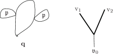
Figure 7. Remark 7.20

The two (almost) bubbles appearing in the figure are supposed to be close to ${\bf q}$. We have two choices (${\bf p},{\bf q},{\rm v}_{1}$) and $({\bf p},{\bf q},{\rm v}_{2})$. Then for these choices the resulting $E_{{\bf p},\vec{\bf q},{\mathfrak{p}};\Xi_{\mathfrak{p}}}({\bf x})$ are supported in the different part of $\Sigma_{\bf x}$ and so are linearly independent in the obstruction bundle datum $E_{\bf p}({\bf x})$ to be defined later.

On the other hand, $E_{{\bf p},\vec{\bf q},{\mathfrak{p}};\Xi_{\mathfrak{p}}}({\bf x})$ is independent of small perturbation of ${\bf p}$.

Lemma 7.21.

Suppose ${\bf p}$, $\vec{\bf q}$, ${\mathfrak{p}}$, $\Xi_{\mathfrak{p}}$ satisfy the assumptions of Lemma 7.16. Then there exists $\mathfrak{o}$ such that if ${\bf p}^{\prime}\in\mathcal{M}_{k+1,\ell}(X,L,J;\beta)$, $d({\bf p},{\bf p}^{\prime})\leq\mathfrak{o}$ then

$$E_{{\bf p},\vec{\bf q},{\mathfrak{p}};\Xi_{\mathfrak{p}}}({\bf x})=E_{{\bf p}^{\prime},\vec{\bf q},{\mathfrak{p}};\Xi_{\mathfrak{p}}}({\bf x})$$

when both sides are defined.

Proof.

By assumption, the added marked points $\vec{\mathfrak{w}}_{{\bf x},{\mathfrak{p}}}$, which are defined by two different choices ${\bf p},\vec{\bf q},{\mathfrak{p}},\Xi_{\mathfrak{p}}$ and ${\bf p}^{\prime},\vec{\bf q},{\mathfrak{p}},\Xi_{\mathfrak{p}}$, are close to each other. Then by applying the Implicit Function Theorem using Lemma 7.16 (2), we derive they coincide. The lemma is a consequence of this fact and the way the space $E_{{\bf p},\vec{\bf q},{\mathfrak{p}};\Xi_{\mathfrak{p}}}({\bf x})$ is defined in (7.16). ∎

8. Existence of a disk-component-wise system of obstruction bundle data 2

In this section we will choose an appropriate set of equivalence classes of the choices of $\vec{\bf q},{\mathfrak{p}},\Xi_{\mathfrak{p}}$ for each ${\bf p}\in\mathcal{M}_{k+1,\ell}(X,L,J;\beta)$, and then the obstruction bundle data $E_{\bf p}({\bf x})$ will be a direct sum of $E_{{\bf p},\vec{\bf q},{\mathfrak{p}};\Xi_{\mathfrak{p}}}({\bf x})$ for such choices. Such an equivalence class will be called a quasi-component. Finding a good choice of a set of quasi-components for each ${\bf p}$ is the main task to carry out.

Definition 8.1.

Let $\mathscr{TC}$ be the set of triples $(k,\ell,\beta)$ such that $k,\ell\in{\mathbb{Z}}_{\geq 0}$, $\beta\in H_{2}(X,L;{\mathbb{Z}})$ and $\mathcal{M}_{k+1,\ell}(X,L,J;\beta)\neq\emptyset$. We define a partial order $<$ on $\mathscr{TC}$ as follows.

Let $(k_{i},\ell_{i},\beta_{i})\in\mathscr{TC}$ ($i=1,2$). We say $(k_{1},\ell_{1},\beta_{1})\,>^{\prime}\,(k_{2},\ell_{2},\beta_{2})$ if there exists ${\bf p}\in\mathcal{M}_{k_{1}+1,\ell_{1}}(X,L,J;\beta_{1})(\mathfrak{T})$ and ${\bf q}\in\mathcal{M}_{k_{2}+1,\ell_{2}}(X,L,J;\beta_{2})$ such that ${\bf q}={\bf p}_{\mathfrak{S}}$ for a certain subtree $\mathfrak{S}$ of $\mathfrak{T}$.

We say $(k,\ell,\beta)>(k^{\prime},\ell^{\prime},\beta^{\prime})$ if there exist $(k_{j},\ell_{j},\beta_{j})$ such that $(k,\ell,\beta)=(k_{1},\ell_{1},\beta_{1})$, $(k^{\prime},\ell^{\prime},\beta^{\prime})=(k_{n},\ell_{n},\beta_{n})$ and $(k_{j},\ell_{j},\beta_{j})\,>^{\prime}\,(k_{j+1},\ell_{j+1},\beta_{j+1})$.

We note that the following is an immediate consequence of Gromov compactness.

Lemma 8.2.

For any $(k,\ell,\beta)\in\mathscr{TC}$, there exists only a finite number of $(k^{\prime},\ell^{\prime},\beta^{\prime})\in\mathscr{TC}$ such that $(k^{\prime},\ell^{\prime},\beta^{\prime})<(k,\ell,\beta)$.

We will associate various objects to $\mathcal{M}_{k+1,\ell}(X,L,J;\beta)$ inductively on this partial order $<$. The objects we will construct are as follows.

1. A finite subset $\mathfrak{P}(k,\ell,\beta)\subset\mathcal{M}^{\circ}_{k+1,\ell}(X,L,J;\beta)$.

2. For each $\mathfrak{p}\in\mathfrak{P}(k,\ell,\beta)$, we take its open neighborhood $K_{\circ}(\mathfrak{p})$ in $\mathcal{M}^{\circ}_{k+1,\ell}(X,L,J;\beta)$ so that its closure $K(\mathfrak{p})$ in $\mathcal{M}^{\circ}_{k+1,\ell}(X,L,J;\beta)$ is a compact subset contained in $\mathcal{M}^{\circ}_{k+1,\ell}(X,L,J;\beta)$.

3. We take type I strong stabilization data together with an obstruction space $E_{\mathfrak{p}}$ at $\mathfrak{p}$, which we denote by $\Xi_{\mathfrak{p}}$.

We will construct other objects $\mathscr{F}_{k+1,\ell,\beta}$, $\mathscr{F}^{\circ}_{k+1,\ell,\beta}$ in addition which will be described later. (See (ob4) right above Condition 8.12.)

We start with describing the conditions we require for them. (Existence of the objects satisfying those conditions will be proved in Proposition 8.18 later.) Let

$$\mathfrak{p}\in\mathfrak{P}(k,\ell,\beta),\qquad{\bf q}\in K(\mathfrak{p}).$$

We require $K(\mathfrak{p})$ to be sufficiently small so that Condition 8.3 below holds. Let $\vec{\mathfrak{w}}_{\mathfrak{p}}$ be the additional interior marked points which are parts of $\Xi_{\mathfrak{p}}$. If $K(\mathfrak{p})$ is sufficiently small, there exists $\vec{w}_{{\bf q},\mathfrak{p}}$ such that ${\bf q}\cup\vec{w}_{{\bf q},\mathfrak{p}}$ is $\epsilon$-close to ${\mathfrak{p}}\cup\vec{\mathfrak{w}}_{\mathfrak{p}}$. In particular,

$$(\Sigma_{\bf q},\vec{w}_{{\bf q},\mathfrak{p}})\in\Phi\left(\mathcal{V}_{{\mathfrak{p}}}^{\rm d}\times\prod_{\mathfrak{v}}\mathcal{V}_{{\mathfrak{p}},{\mathfrak{v}}}^{\rm s}\times(D^{2}(c))^{m_{\rm s}}\right)$$ (8.1)

where $\Phi$ is the map (7.6) induced by $\Xi_{\mathfrak{p}}$. Therefore in the same way as in Section 7, we obtain an embedding

$$\hat{\Phi}_{{\bf q},{\mathfrak{p}};\Xi_{\mathfrak{p}}}:\rm{Supp}(E_{\mathfrak{p}})\to\Sigma_{\bf q}$$ (8.2)

and then a map

$$\mathcal{P}_{{\bf q},{\mathfrak{p}};\Xi_{\mathfrak{p}}}: C^{2}(\hat{\Phi}_{{\bf q},{\mathfrak{p}};\Xi_{\mathfrak{p}}}(U({\rm Supp}(E_{\mathfrak{p}}))),u_{\bf q}^{*}TX\otimes\Lambda^{0,1})$$ (8.3)

$$\to C^{2}(U({\rm Supp}(E_{\mathfrak{p}})),u_{\mathfrak{p}}^{*}TX\otimes\Lambda^{0,1})$$

where $U({\rm Supp}(E_{\mathfrak{p}}))$ is a sufficiently small open neighborhood of ${\rm Supp}(E_{\mathfrak{p}})$. Then we define

$$E_{{\bf q},{\mathfrak{p}};\Xi_{\mathfrak{p}}}({\bf q})=(\mathcal{P}_{{\bf q},{\mathfrak{p}};\Xi_{\mathfrak{p}}})^{-1}(E_{\mathfrak{p}}).$$ (8.4)

Condition 8.3.

We require that $K(\mathfrak{p})$ is so small that (8.1) holds, (8.2),(8.3) are well defined, and Definition 7.6 (2)(3) hold with $E_{\mathfrak{p}}$ replaced by $E_{{\bf q},{\mathfrak{p}};\Xi_{\mathfrak{p}}}({\bf q})$.

We remark that if ${\mathfrak{p}}={\bf q}$ then Definition 7.6 (2)(3) hold by assumption. Therefore Condition 8.3 holds if $K(\mathfrak{p})$ is sufficiently small.

We denote by $\mathfrak{T}_{0}\in\mathcal{G}(k+1,\ell,\beta)$ the unique element that has only one interior vertex. We call it the trivial element.

Now we will discuss the relationship between the data given above and the construction of Subsection 7.3. Suppose we are given a finite set $\mathfrak{P}(k,\ell,\beta)$ as in (ob1) for each $(k,\ell,\beta)$ and $\Xi_{\mathfrak{p}}$ as in (ob3) for $\mathfrak{p}\in\mathfrak{P}(k,\ell,\beta)$.

Situation 8.4.

We consider ${\bf p}$, ${\bf q}_{j}$, ${\mathfrak{p}}$, $\mathfrak{T}_{j}$, $\mathfrak{S}_{j}$ ($j=1,\dots,n$ for some $n\geq 1$) as in Situation 7.15, except we require

1. $d({\bf p},{\bf q}_{1})<\epsilon(k,\ell,\beta)=\epsilon(k_{1},\ell_{1},\beta_{1})$.

2. For $j\leq n-1$ we require ${\bf q}_{j,\mathfrak{S}_{j}}\in\mathcal{M}_{k_{j+1}+1,\ell_{j+1}}(X,L,J;\beta_{j+1})$ and

   $$d({\bf q}_{j,\mathfrak{S}_{j}},{\bf q}_{j+1})<\epsilon(k_{j+1},\ell_{j+1},\beta_{j+1}).$$ (8.5)

3. ${{\mathfrak{p}}}\in\mathfrak{P}(k_{n+1},\ell_{n+1},\beta_{n+1})$, ${\bf q}_{n,{\mathfrak{S}}_{n}}\in\mathcal{M}_{k_{n+1}+1,\ell_{n+1}}(X,L,J;\beta_{n+1})$, and

   $$d({\bf q}_{n,\mathfrak{S}_{n}},\mathfrak{p})<\epsilon(\mathfrak{p})$$

instead of (3), (5), (6).

Here $\epsilon(k,\ell,\beta)$ is a sufficiently small positive number depending only on $k,\ell,\beta$, and the set $\mathfrak{P}(k^{\prime},\ell^{\prime},\beta^{\prime})$ with $(k,\ell,\beta)>(k^{\prime},\ell^{\prime},\beta^{\prime})$, and $\epsilon(\mathfrak{p})$ is a positive number depending only on $\mathfrak{p}$, $\Xi_{\mathfrak{p}}$. They are to be determined later during the proof of Lemma 8.5.

In case $n=0$ we assume

$$d({\bf p},\mathfrak{p})<\epsilon(\mathfrak{p}).$$ (8.6)

We require that (8.6) implies ${\bf p}\in K_{0}(\mathfrak{p})$. $\diamond$

We consider ${\bf x}\in B_{\epsilon_{0}}(\mathcal{X},{\bf p})$. (Here $\epsilon_{0}$ depends on ${\bf p}$ etc. and will be determined later.) Note that the conditions on the distance appearing in (3)’,(5)’,(6)’ are similar to but slightly different from (3),(5),(6) in Situation 7.15. The next lemma claims that we can use (3)’,(5)’,(6)’ in place of (3),(5),(6).

Lemma 8.5.

Suppose $n\geq 1$ in Situation 8.4. We may choose $\epsilon(k,\ell,\beta)$ so that if (1),(2),(3)’,(4),(5)’,(6)’,(7) above hold then the conclusions of Lemmas 7.17,7.18 hold with the right hand sides of (7.22),(7.25) replaced by $\delta(\mathfrak{p})$ in (7.23).

In case $n=0$ the same conclusion holds under the assumption (8.6).

Namely, Lemma 8.5 claims uniformity of the constants $\epsilon_{1,j}(\delta;{\bf q}_{j},\dots,{\bf q}_{n},{\mathfrak{p}},\Xi_{\mathfrak{p}})$ and $\epsilon_{2}(\delta;{\mathfrak{p}},\Xi_{\mathfrak{p}})$. In (7.20) they depend on ${\bf p},{\bf q}_{1},\dots,{\bf q}_{n},\mathfrak{p}$. However, Lemma 8.5 asserts that we can choose them so that they depend only on $k_{j}$, $\ell_{j}$, $\beta_{j}$ and that the conclusions of Lemmas 7.16, 7.17 and 7.18 hold. We prove this technical Lemma 8.5 at the end of this section using compactness of various spaces.

Now we apply Lemma 7.16 to obtain $\vec{\mathfrak{w}}_{{\bf x};{\mathfrak{p}}}$, $\vec{\mathfrak{w}}_{{\bf p};{\mathfrak{p}}}$ $\vec{\mathfrak{w}}_{{\bf q}_{j},{\mathfrak{p}}}$ ($j=1,\dots,n$). Then we use Lemma 7.17 to obtain smooth embeddings

$$\widehat{\Phi}_{{\bf x},{\bf p},\vec{\bf q},{\mathfrak{p}};\Xi_{\mathfrak{p}}}:{\rm Supp}(E_{\mathfrak{p}})\to\Sigma_{{\bf x}}$$ (8.7)

as in (7.7). Note $\vec{\mathfrak{w}}_{{\bf p};{\mathfrak{p}}}$ also depends on $\vec{\bf q}$ so we write $\vec{\mathfrak{w}}_{{\bf p},\vec{\bf q};{\mathfrak{p}}}$. Then Lemma 8.5 enables us to define the following notion.

Definition 8.6.

We call $({\bf p},\vec{\bf q},\mathfrak{p};\vec{\mathfrak{T}},\vec{\mathfrak{S}})$ as in Situation 8.4 a quasi-splitting sequence. Suppose $({\bf p},\vec{\bf q}_{(c)},\mathfrak{p};\vec{\mathfrak{T}}_{(c)},\vec{\mathfrak{S}}_{(c)})$ for $c=1,2$ are quasi-splitting sequences (with the same ${\bf p},\mathfrak{p}$). We say that they are equivalent if

$$\vec{\mathfrak{w}}_{{\bf p},\vec{\bf q}_{(1)},{\mathfrak{p}}}=\vec{\mathfrak{w}}_{{\bf p},\vec{\bf q}_{(2)},{\mathfrak{p}}}.$$

An equivalence class of quasi-splitting sequences is called a quasi-component.

Let ${\mathscr{QC}}_{k+1,\ell}(X,L,J;\beta)$ be the set of all quasi-components. There is a map

$$\Pi=\Pi_{\beta}:{\mathscr{QC}}_{k+1,\ell}(X,L,J;\beta)\to\mathcal{M}_{k+1,\ell}(X,L,J;\beta)$$ (8.8)

which assigns ${\bf p}$ to an equivalence class of $({\bf p},\vec{\bf q},\mathfrak{p};\vec{\mathfrak{T}},\vec{\mathfrak{S}})$. We say an element $\xi$ of ${\mathscr{QC}}_{k+1,\ell}(X,L,J;\beta)$ is a quasi-component of ${\bf p}$ if $\Pi(\xi)={\bf p}$. We write an element of ${\mathscr{QC}}_{k+1,\ell}(X,L,J;\beta)$ as

$$({\bf p},\xi,\mathfrak{p})$$

where ${\bf p}$ and ${\mathfrak{p}}$ are the first and the last element of the sequence. We put

$$\vec{\mathfrak{w}}_{{\bf p},\xi,\mathfrak{p}}=\vec{\mathfrak{w}}_{{\bf p},\vec{\bf q},{\mathfrak{p}}}$$

if $\xi$ is the equivalence class of $({\bf p},\vec{\bf q},{\mathfrak{p}};\vec{\mathfrak{T}},\vec{\mathfrak{S}})$.

We note that

$$\widehat{\Phi}_{{\bf x},{\bf p},\vec{\bf q}_{(1)},{\mathfrak{p}};\Xi_{\mathfrak{p}}}=\widehat{\Phi}_{{\bf x},{\bf p},\vec{\bf q}_{(2)},{\mathfrak{p}};\Xi_{\mathfrak{p}}},$$

if $({\bf p},\vec{\bf q}_{(1)},{\mathfrak{p}};\vec{\mathfrak{T}}_{(1)},\vec{\mathfrak{S}}_{(1)})$ is equivalent to $({\bf p},\vec{\bf q}_{(2)},{\mathfrak{p}};\vec{\mathfrak{T}}_{(2)},\vec{\mathfrak{S}}_{(2)})$. Therefore for each quasi-component $({\bf p},\xi,\mathfrak{p})$ we can associate an embedding

$$\widehat{\Phi}_{({\bf x},{\bf p},\xi,\mathfrak{p})}:{\rm Supp}(E_{\mathfrak{p}})\to\Sigma_{{\bf x}}.$$ (8.9)

It then induces a map

$$\mathcal{P}_{({\bf x},{\bf p},\xi,\mathfrak{p})}: C^{2}(\widehat{\Phi}_{({\bf x},{\bf p},\xi,\mathfrak{p})}(U({\rm Supp}(E_{\mathfrak{p}})));u_{\bf x}^{*}TX\otimes\Lambda^{0,1})$$ (8.10)

$$\to C^{2}(U({\rm Supp}(E_{\mathfrak{p}}));u^{*}_{\mathfrak{p}}TX\otimes\Lambda^{0,1})$$

in the same way as (7.27). We define

$$E_{{\bf p},\xi,{\mathfrak{p}}}({\bf x})=(\mathcal{P}_{({\bf x},{\bf p},\xi,\mathfrak{p})})^{-1}(E_{\mathfrak{p}}).$$ (8.11)

Compare this with (7.28). Here $E_{\mathfrak{p}}$ is a part of the data $\Xi_{\mathfrak{p}}$.

The obstruction bundle data $\{E_{{\bf p}}({\bf x})\}$ we will construct are the direct sum of $E_{{\bf p},\xi,{\mathfrak{p}}}({\bf x})$ for an appropriate set of quasi-components of ${\bf p}$. We need a careful choice of the set of the quasi-components so that it satisfies the required properties. The discussion of the process of choosing such a set of quasi-components will follow. We first observe:

Lemma 8.7.

For each ${\bf p}\in\mathcal{M}_{k+1,\ell}(X,L,J;\beta)$, the set $\Pi^{-1}({\bf p})$ of quasi-components of ${\bf p}$ is a finite set.

Proof.

It follows from Lemma 7.8 and the transversality imposed on $\mathcal{N}_{\mathfrak{p},i}$ in Definition 7.3 that each $\mathfrak{w}_{\mathfrak{p},i}$ carries its sufficiently small connected neighborhood $U_{i}\subset\Sigma_{\mathfrak{p}}$ such that $U_{i}\cap\vec{\mathfrak{w}}_{\mathfrak{p}}$ is a single point, i.e.,

$$U_{i}\cap\vec{\mathfrak{w}}_{\mathfrak{p}}=\{\mathfrak{w}_{\mathfrak{p},i}\}$$

and $u_{\bf p}\circ\widehat{\Phi}_{({\bf p},\xi,\mathfrak{p})}:U_{i}\to X$ and $u_{\mathfrak{p}}:U_{i}\to X$ are $C^{2}$-close embeddings for all possible such choices $({\bf p},\xi,\mathfrak{p})$. Here and hereafter we denote $\widehat{\Phi}_{({\bf p},\xi,\mathfrak{p})}=\widehat{\Phi}_{({\bf p},{\bf p},\xi,\mathfrak{p})}$ and the right hand side is the case ${\bf p}={\bf x}$ of (8.9). Recall that, for given ${\bf p}$, the number of possible objects $\mathfrak{p}$ which appear in the quasi-component $({\bf p},\xi,\mathfrak{p})$ of ${\bf p}$ is finite by Lemma 8.2 and finiteness of $\mathfrak{P}(k,\ell,\beta)$.

For any $({\bf p},\xi,\mathfrak{p})$, we put $U^{\prime}_{i,\xi}=\widehat{\Phi}_{({\bf p},\xi,\mathfrak{p})}(U_{i})$. Then by the above mentioned $C^{2}$-closeness we have

$$\int_{U^{\prime}_{i,\xi}}u_{\bf p}^{*}\omega_{X}>\frac{1}{2}\int_{U_{i}}u_{\mathfrak{p}}^{*}\omega_{X}>c$$ (8.12)

for some positive number $c$ independent of $i,\xi$.

Now consider two different quasi-components $({\bf p},\xi,\mathfrak{p})$ and $({\bf p},\xi^{\prime},\mathfrak{p})$. We put $U^{\prime}_{i,\xi^{\prime}}=\widehat{\Phi}_{({\bf p},\xi^{\prime},\mathfrak{p})}(U_{i})$ similarly as $U^{\prime}_{i,\xi}$. Then there exists $i$ such that

$${\mathfrak{w}}_{{\bf p},\xi,\mathfrak{p},i}\neq{\mathfrak{w}}_{{\bf p},\xi^{\prime},\mathfrak{p},i},\quad{\mathfrak{w}}_{{\bf p},\xi,\mathfrak{p},i}\in U^{\prime}_{i,\xi},\,{\mathfrak{w}}_{{\bf p},\xi^{\prime},\mathfrak{p},i}\in U^{\prime}_{i,\xi^{\prime}}$$ (8.13)

by the definition of the equivalence class $\xi$. It follows from the $C^{2}$-closeness of $u_{\bf p}\circ\widehat{\Phi}_{({\bf p},\xi,\mathfrak{p})}$ and $u_{\bf p}\circ\widehat{\Phi}_{({\bf p},\xi^{\prime},\mathfrak{p})}$, the transversality imposed on $\mathcal{N}_{\mathfrak{p},i}$ and the embedding properties of $\widehat{\Phi}_{({\bf p},\xi,\mathfrak{p})}$, $\widehat{\Phi}_{({\bf p},\xi,\mathfrak{p})}$ that we have a covering map

$$(\widehat{\Phi}_{({\bf p},\xi,\mathfrak{p})})^{-1}\cup(\widehat{\Phi}_{({\bf p},\xi^{\prime},\mathfrak{p})})^{-1}:U^{\prime}_{i,\xi}\cup U^{\prime}_{i,\xi^{\prime}}\to U_{i}$$

which is a homeomorphism on each of $U^{\prime}_{i,\xi}$ and on $U^{\prime}_{i,\xi^{\prime}}$ respectively. Therefore (8.13) implies $U^{\prime}_{i,\xi}\cap U^{\prime}_{i,\xi^{\prime}}=\emptyset$. This clearly implies that the number of such $({\bf p},\xi,\mathfrak{p})$ must be finite. In fact otherwise we would have

$$\infty>\int_{\Sigma_{\bf p}}u_{\bf p}^{*}\omega_{X}\geq\sum_{({\bf p},\xi,\mathfrak{p})}\int_{U^{\prime}_{i,\xi}}u_{\bf p}^{*}\omega_{X}=\infty,$$

a contradiction. Here we use (8.12). This finishes the proof. ∎

Let $\mathscr{F}$ be a subset of ${\mathscr{QC}}_{k+1,\ell}(X,L,J;\beta)$. For a given point ${\bf p}\in\mathcal{M}_{k+1,\ell}(X,L,J;\beta)$ we put

$$\mathscr{F}({\bf p})=\Pi^{-1}({\bf p})\cap\mathscr{F},$$

which is a finite set. In this way we regard the assignment $\mathscr{F}:{\bf p}\mapsto\mathscr{F}({\bf p})$ as a map which assigns a finite set of quasi-components of ${\bf p}$ to an element ${\bf p}$ of ${\mathcal{M}}_{k+1,\ell}(X,L,J;\beta)$. We call $\mathscr{F}$ a quasi-component choice map.

We next define a topology on ${\mathscr{QC}}_{k+1,\ell}(X,L,J;\beta)$ using the next lemma.

Let ${\bf p}\in\mathcal{M}_{k+1,\ell}(X,L,J;\beta)$. We fix a stabilization and trivialization data at ${\bf p}$ in the sense of [FOOO8, Definition 4.9]. Then if ${\bf p}^{\prime}\in\mathcal{M}_{k+1,\ell}(X,L,J;\beta)$ is close to ${\bf p}$, we can define a map $\hat{\Phi}_{{\bf p}^{\prime}{\bf p}}:\Sigma_{\bf p}(\vec{\epsilon})\to\Sigma_{{\bf p}^{\prime}}$. (See [FOOO8, Lemma 3.9].)

Lemma 8.8.

There are neighborhoods $U({\bf p})$ of ${\bf p}$ in $\mathcal{M}_{k+1,\ell}(X,L,J;\beta)$ and $U({\mathfrak{w}}_{{\bf p},\xi,{\mathfrak{p}},i})$ of ${\mathfrak{w}}_{{\bf p},\xi,{\mathfrak{p}},i}$ in $\Sigma_{\bf p}$ such that if ${\bf p}^{\prime}\in U({\bf p})$ and $({\bf p},\xi,\mathfrak{p})$ is an quasi-component of ${\bf p}$, and there exists a unique quasi-component $({\bf p}^{\prime},\xi^{\prime},\mathfrak{p})$ of ${\bf p}^{\prime}$ with the same ${\mathfrak{p}}$ such that ${\mathfrak{w}}_{{\bf p}^{\prime},\xi^{\prime},{\mathfrak{p}},i}\in\hat{\Phi}_{{\bf p}^{\prime}{\bf p}}(U({\mathfrak{w}}_{{\bf p},\xi,{\mathfrak{p}},i}))$.

Proof.

Let $({\bf p},\vec{\bf q},\mathfrak{p})$ be a quasi-splitting sequence representing $({\bf p},\xi,\mathfrak{p})$. It follows from definition that $({\bf p}^{\prime},\vec{\bf q},\mathfrak{p})$ is also a quasi-splitting sequence if ${\bf p}^{\prime}$ is sufficiently close to ${\bf p}$. We thus obtain $({\bf p}^{\prime},\xi^{\prime},\mathfrak{p})$.

The quasi-component $\xi^{\prime}$ is independent of the choice of a representative of $\xi$ because the point ${\mathfrak{w}}_{{\bf p}^{\prime},\xi^{\prime},{\mathfrak{p}},i}$ which is close to ${\mathfrak{w}}_{{\bf p},\xi,{\mathfrak{p}},i}$ and $u_{{\bf p}^{\prime}}({\mathfrak{w}}_{{\bf p}^{\prime},\xi^{\prime},{\mathfrak{p}},i})\in\mathcal{N}_{{\mathfrak{p}},i}$ is unique. The uniqueness in the statement of Lemma 8.8 follows from the same fact. ∎

Definition 8.9.

We define a topology on ${\mathscr{QC}}_{k+1,\ell}(X,L,J;\beta)$ as follows.

Let $({\bf p},\xi,\mathfrak{p})\in{\mathscr{QC}}_{k+1,\ell}(X,L,J;\beta)$. By Lemma 8.8 we obtain a neighborhood $U({\bf p})$ and an injective map $U({\bf p})\to{\mathscr{QC}}_{k+1,\ell}(X,L,J;\beta)$ which sends ${\bf p}^{\prime}$ to $({\bf p}^{\prime},\xi,\mathfrak{p})$. We define a neighborhood system of $({\bf p},\xi,\mathfrak{p})$ by sending one of ${\bf p}$ by this map.

Lemma 8.10.

This topology is Hausdorff. The map $\Pi:{\mathscr{QC}}_{k+1,\ell}(X,L,J;\beta)\to\mathcal{M}_{k+1,\ell}(X,L,J;\beta)$ is a local homeomorphism. Namely for each point ${\mathfrak{x}}\in{\mathscr{QC}}_{k+1,\ell}(X,L,J;\beta)$ there exist neighborhoods of $\mathfrak{x}$ and of $\Pi(\mathfrak{x})$ so that $\Pi$ induces a homeomorphism between them.

The proof is easy and is omitted.

Definition 8.11.

A quasi-component choice map $\mathscr{F}$ is said to be open (resp. closed) if it is open (resp. closed) as a subset of ${\mathscr{QC}}_{k+1,\ell}(X,L,J;\beta)$.

The closure of a quasi-component choice map is defined to be the closure as a subset of ${\mathscr{QC}}_{k+1,\ell}(X,L,J;\beta)$.

$\mathscr{F}$ is said to be proper if the restriction of $\Pi$ to $\mathscr{F}$ is a proper map (to $\mathcal{M}_{k+1,\ell}(X,L,J;\beta)$).

Other objects mentioned right after Lemma 8.2 we will construct are:

1. Quasi-component choice maps $\mathscr{F}^{\circ}_{k+1,\ell,\beta}$ and $\mathscr{F}_{k+1,\ell,\beta}$ for each $(k,\ell,\beta)\in\mathscr{TC}$.

We describe the conditions we require for $\mathscr{F}^{\circ}_{k+1,\ell,\beta}$ and $\mathscr{F}_{k+1,\ell,\beta}$ below.

Condition 8.12.

$\mathscr{F}^{\circ}_{k+1,\ell,\beta}$ is open. $\mathscr{F}_{k+1,\ell,\beta}$ contains its closure and is proper. $\mathscr{F}^{\circ}_{k+1,\ell,\beta}$ and $\mathscr{F}_{k+1,\ell,\beta}$ are invariant under the action of extended automorphism group in an obvious sense.

We require three more conditions. The first one is Condition 8.13 which describes $\mathscr{F}^{\circ}_{k+1,\ell,\beta}$, $\mathscr{F}_{k+1,\ell,\beta}$ at the boundary points of $\mathcal{M}_{k+1,\ell}(X,L,J;\beta)$. Let ${\bf p}\in\mathcal{M}_{k+1,\ell}^{\circ}(X,L,J;\beta)(\mathfrak{T})$ where $\mathfrak{T}=({\mathcal{T}},\beta(\cdot),l(\cdot))$ is nontrivial, i.e., $\mathcal{T}$ has at least two interior vertices. (See Definition 2.13 and (4.5) for this notation.) For an interior vertex ${\rm v}$ of $\mathcal{T}$, we obtain ${\bf p}_{\rm v}\in\mathcal{M}_{k_{\rm v}+1,\ell_{\rm v}}^{\circ}(X,L,J;\beta({\rm v}))$. Let us define a map

$$\mathscr{I}_{{\bf p},{\rm v}}:\Pi_{\beta({\rm v})}^{-1}({\bf p}_{\rm v})\to\Pi^{-1}_{\beta}({\bf p}).$$ (8.14)

Note that $\Pi_{\beta}$, $\Pi_{\beta({\rm v})}$ are the maps (8.8) and $\Pi_{\beta}^{-1}({\bf p}_{\rm v})$ is the set of all quasi-components of ${\bf p}_{\rm v}$. Consider a quasi-component $({\bf p}_{\rm v},\xi,\mathfrak{p};\vec{\mathfrak{T}},\vec{\mathfrak{S}})$ of ${\bf p}_{\rm v}$. We put $\mathfrak{S}^{\prime}_{1}=\{{\rm v}\}$ and ${\bf q}^{\prime}_{1}={\bf p}_{\rm v}$. If $\xi$ is represented by a sequence ${\bf q}_{i}$, $\mathfrak{S}_{i}$, we put ${\bf q}^{\prime}_{i+1}={\bf q}_{i}$ and shift the index of $\vec{\mathfrak{S}}$ by $1$ to obtain $\vec{\mathfrak{S}}^{\prime}$. $\vec{\mathfrak{T}}^{\prime}$ is obtained from ${\bf q}^{\prime}_{i}$ automatically. We thus obtain a quasi-component $({\bf p},\xi^{\prime},\mathfrak{p};\vec{\mathfrak{T}}^{\prime},\vec{\mathfrak{S}}^{\prime})$ of ${\bf p}$. We define

$$\mathscr{I}_{{\bf p},{\rm v}}({\bf p}_{\rm v},\xi,\mathfrak{p};\vec{\mathfrak{T}},\vec{\mathfrak{S}}):=({\bf p},\xi^{\prime},\mathfrak{p};\vec{\mathfrak{T}}^{\prime},\vec{\mathfrak{S}}^{\prime}).$$

Condition 8.13.

(Boundary stratifications) For ${\bf p}\in\mathcal{M}_{k+1,\ell}^{\circ}(X,L,J;\beta)(\mathfrak{T})$ with nontrivial $\mathfrak{T}=({\mathcal{T}},\beta(\cdot),l(\cdot))$, $\mathscr{F}^{\circ}_{k+1,\ell,\beta}({\bf p})$ is the set of all equivalence classes of quasi-components $({\bf p},\xi^{\prime},\mathfrak{p})$ as above, where we take all possible choices of ${\rm v}$ and $({\bf p}_{\rm v},\xi,\mathfrak{p})\in\mathscr{F}^{\circ}_{k_{\rm v},\ell_{\rm v},\beta({\rm v})}({\bf p}_{\rm v})$. In other words, we have

$$\mathscr{F}^{\circ}_{k+1,\ell,\beta}({\bf p})=\bigcup_{{\rm v}\in C_{0}^{\rm int}(\mathcal{T})}\mathscr{I}_{{\bf p},{\rm v}}(\mathscr{F}^{\circ}_{k_{\rm v}+1,\ell_{\rm v},\beta_{\rm v}}({\bf p}_{\rm v})).$$ (8.15)

The same holds if we replace $\mathscr{F}^{\circ}$ by $\mathscr{F}$. Namely, we have

$$\mathscr{F}_{k+1,\ell,\beta}({\bf p})=\bigcup_{{\rm v}\in C_{0}^{\rm int}(\mathcal{T})}\mathscr{I}_{{\bf p},{\rm v}}(\mathscr{F}_{k_{\rm v}+1,\ell_{\rm v},\beta_{\rm v}}({\bf p}_{\rm v})).$$ (8.16)

It is easy to see that both of the right hand sides of (8.15) and (8.16) are disjoint unions.

The remaining two conditions we require are related to transversality. For ${\bf p}\in\mathcal{M}_{k+1,\ell}(X,L,J;\beta)$ we consider the sum:

$$\sum_{({\bf p},\xi,\mathfrak{p})\in\mathscr{F}_{k+1,\ell,\beta}({\bf p})}E_{{\bf p},\xi,{\mathfrak{p}}}({\bf p})\subset C^{\infty}(\Sigma_{\bf p};u_{\bf p}^{*}TX\otimes\Lambda^{0,1}).$$ (8.17)

Here we note that we have

$$\widehat{\Phi}_{({\bf p},{\bf p},\xi,{\mathfrak{p}})}(U(\text{\rm Supp}(E_{{\mathfrak{p}}})))\subset\Sigma_{\bf p}$$

in (8.9) with ${\bf x}={\bf p}$.

Condition 8.14.

(Direct sum) The sum (8.17) is a direct sum which we denote by:

$$E_{{\bf p};\mathscr{F}}({\bf p})=\bigoplus_{({\bf p},\xi,\mathfrak{p})\in\mathscr{F}_{k+1,\ell,\beta}({\bf p})}E_{{\bf p},\xi,{\mathfrak{p}}}({\bf p})\subset C^{\infty}(\Sigma_{\bf p};u_{\bf p}TX\otimes\Lambda^{0,1}).$$ (8.18)

For a given point ${\bf p}\in\mathcal{M}_{k+1,\ell}(X,L,J;\beta)$, we may take $\epsilon_{0}({\bf p})>0$ so small that if ${\bf x}\in B_{\epsilon_{0}({\bf p})}(\mathcal{X},{\bf x})$, the subspace $E_{{\bf p},\xi,{\mathfrak{p}}}({\bf x})$ as in (8.11) is defined and we have the sums

$$E_{{\bf p};\mathscr{F}}({\bf x}) =\bigoplus_{({\bf p},\xi,\mathfrak{p})\in\mathscr{F}_{k+1,\ell,\beta}({\bf p})}E_{{\bf p},\xi,{\mathfrak{p}}}({\bf x})\subset C^{2}(\Sigma_{\bf x};u_{\bf x}TX\otimes\Lambda^{0,1}),$$

$$E_{{\bf p};\mathscr{F}}^{\circ}({\bf x}) =\bigoplus_{({\bf p},\xi,\mathfrak{p})\in\mathscr{F}^{\circ}_{k+1,\ell,\beta}({\bf p})}E_{{\bf p},\xi,{\mathfrak{p}}}({\bf x})\subset C^{2}(\Sigma_{\bf x};u_{\bf x}TX\otimes\Lambda^{0,1}).$$

Note that the sums in the right hand sides are direct sums by Condition 8.14.

Condition 8.15.

(Transversality) We consider the operator

$$D_{u_{\bf p}}\overline{\partial}:W^{2}_{m+1}((\Sigma_{\bf p},\partial\Sigma_{\bf p});u_{\bf p}^{*}TX,u_{\bf p}^{*}TL)\to L^{2}_{m}(\Sigma_{\bf p},u_{\bf p}^{*}TX\otimes\Lambda^{0,1})$$

as in [FOOO8, (5.1)]. Then we require

$${\rm Im}D_{u_{\bf p}}\overline{\partial}+E^{\circ}_{{\bf p};\mathscr{F}}({\bf p})=L^{2}_{m}(\Sigma,u_{\bf p}^{*}TX\otimes\Lambda^{0,1}).$$

Moreover for the evaluation map

$${\mathcal{EV}}:W^{2}_{m+1}((\Sigma_{\bf p},\partial\Sigma_{\bf p});u_{\bf p}^{*}TX,u_{\bf p}^{*}TL)\to T_{u_{\bf p}(z_{0})}L$$

at $z_{0}$, the restriction

$${\mathcal{EV}}:(D_{u_{\bf p}}\overline{\partial})^{-1}(E^{\circ}_{{\bf p};\mathscr{F}}({\bf p}))\to T_{u_{\bf p}(z_{0})}L$$

is surjective, and the action of ${\rm Aut}({\bf p})$ on $(D_{u_{\bf p}}\overline{\partial})^{-1}(E^{\circ}_{{\bf p};\mathscr{F}}({\bf p}))/{\mathfrak{aut}}(\Sigma_{\bf p},\vec{z}_{\bf p},\vec{\mathfrak{z}}_{\bf p})$ is effective.

Remark 8.16.

Note that in case $D_{u_{\bf p}}\overline{\partial}$ is not surjective, Condition 8.15 implies that $\mathscr{F}^{\circ}_{k+1,\ell,\beta}({\bf p})$ is non-empty. We may take $E^{\circ}_{{\mathbf{p}},{\mathcal{F}}}=0$, when $D_{u_{\mathbf{p}}}\overline{\partial}$ is surjective and the restriction of $\mathcal{EV}$ to $\rm{Ker}\,D_{u_{\mathbf{p}}}\overline{\partial}$ is surjective.

Now we have the following two results.

Proposition 8.17.

Suppose we have the objects as in (ob1)-(ob4) and the constants $\epsilon(k,\ell,\beta)>0$, $\epsilon(\mathfrak{p})>0$ such that Conditions 8.3, 8.12, 8.13, 8.14, 8.15 are satisfied and that $\epsilon(k,\ell,\beta)$, $\epsilon(\mathfrak{p})>0$ are as in Lemma 8.5. Then we can choose $\epsilon_{0}({\bf p})>0$ for each ${\bf p}$ such that $\mathscr{U}_{\bf p}=B_{\epsilon_{0}({\bf p})}(\mathcal{X},{\bf p})$ and $\{E_{{\bf p};\mathscr{F}}({\bf x})\}$ is a system of obstruction bundle data that is disk-component-wise.

Proposition 8.18.

There exist objects as in (ob1)-(ob4) and constants $\epsilon(k,\ell,\beta)>0$, $\epsilon(\mathfrak{p})>0$ such that Conditions 8.3, 8.12, 8.13, 8.14, 8.15 are satisfied and $\epsilon(k,\ell,\beta)$, $\epsilon(\mathfrak{p})>0$ are as in Lemma 8.5.

It is obvious that Propositions 8.17 and 8.18 imply Theorem 5.4. Thus to prove Theorem 5.4 it remains to prove Propositions 8.17 and 8.18 and Lemma 8.5.

Proof of Proposition 8.17.

We first check that $\{E_{{\bf p};\mathscr{F}}({\bf x})\}$ is an obstruction bundle data. Definition 3.1 (1) is obvious from construction. Definition 3.1 (2) (smoothness) is a consequence of Lemma 7.19.

Definition 3.1 (3) (transversality) is a consequence of Condition 8.15 for ${\bf x}={\bf p}$. By taking $\epsilon_{0}({\bf p})>0$ small enough, we can prove the same property for ${\bf x}\in B_{\epsilon_{0}({\bf p})}(\mathcal{X},{\bf p})$.

Definition 3.1 (4) (semi-continuity) is a consequence of Lemma 7.21 and the properness of $\mathscr{F}_{k+1,\ell,\beta}$, which is a part of Condition 8.12. Definition 3.1 (5) (invariance under the extended automorphisms) is a consequence of the invariance of $\mathscr{F}_{k+1,\ell,\beta}$, which is a part of Condition 8.12.

We then observe that disk-component-wise-ness (5.1) is an immediate consequence of Condition 8.13 and the definition. ∎

Proof of Proposition 8.18.

The proof is by induction on $(k,\ell,\beta)$ with respect to the partial order $<$. We first consider the case when $(k,\ell,\beta)$ is minimal. In this case $\mathcal{G}(k+1,\ell,\beta)$ consists of one element, the trivial element $\mathfrak{T}_{0}$. We can construct $\mathfrak{P}(k,\ell,\beta)$, $\Xi_{\mathfrak{p}}$ and $K_{\circ}({\mathfrak{p}})$ for its element $\mathfrak{p}$ in the same way as in [FOOO8, Section 11]. In fact, the set $\mathfrak{P}(k,\ell,\beta)$ is the set $\{{\bf p}_{1},\dots,{\bf p}_{\mathscr{P}}\}$ appearing right above [FOOO8, (11.7)]. Here $K_{\circ}(\mathfrak{p})$ is the same as that of [FOOO8, Section 11]. Condition 8.3 is obviously satisfied from construction.

In this case, ${\mathscr{QC}}_{k+1,\ell}(X,L,J;\beta)$ consists of the pair $({\bf p},\mathfrak{p})$ such that ${\bf p}\in K_{\circ}(\mathfrak{p})$. We define ${\mathscr{F}}_{k+1,\ell,\beta}$ as follows. We take compact subsets $K_{-}(\mathfrak{p})\subset K_{\circ}(\mathfrak{p})$ such that

$$\bigcup_{\mathfrak{p}}{\rm Int}K_{-}(\mathfrak{p})=\mathcal{M}_{k+1,\ell}(X,L,J;\beta).$$ (8.19)

We then put

$${\mathscr{F}}^{\circ}_{k+1,\ell,\beta}({\bf p}) =\{({\bf p},\mathfrak{p})\mid{\bf p}\in{\rm Int}K_{-}(\mathfrak{p})\},$$

$${\mathscr{F}}_{k+1,\ell,\beta}({\bf p}) =\{({\bf p},\mathfrak{p})\mid{\bf p}\in K_{-}(\mathfrak{p})\}.$$

Condition 8.12 is immediate. Condition 8.13 is void in this case. Note that $({\bf p},\mathfrak{p})$ is the case $n=0$ of Situation 7.15.

In the same way as [FOOO8, Lemma 11.7] we can perturb $E_{\mathfrak{p}}$ by an arbitrary small amount so that Condition 8.14 holds. Condition 8.15 is a consequence of (8.19). We have thus completed the proof for the minimal $(k,\ell,\beta)$, that is the first step of the induction.

Next, we assume that we have already obtained $\mathscr{F}^{\circ}_{k^{\prime}+1,\ell^{\prime},\beta^{\prime}}$ and $\mathscr{F}_{k^{\prime}+1,\ell^{\prime},\beta^{\prime}}$ satisfying the required conditions for all $(k^{\prime},\ell^{\prime},\beta^{\prime})$ with $(k^{\prime},\ell^{\prime},\beta^{\prime})<(k,\ell,\beta)$. We will prove the same conclusion for the case of $\mathscr{F}^{\circ}_{k+1,\ell,\beta}$ and $\mathscr{F}_{k+1,\ell,\beta}$.

We will first define an open subset $\mathscr{F}^{\circ\prime}_{k+1,\ell,\beta}$ and a compact subset $\mathscr{F}^{\prime}_{k+1,\ell,\beta}$ of ${\mathscr{QC}}_{k+1,\ell}(X,L,J;\beta)$. After that, we will modify them to obtain the desired $\mathscr{F}^{\circ}_{k+1,\ell,\beta}$ and $\mathscr{F}_{k+1,\ell,\beta}$.

First we consider the case ${\bf p}\in\partial\mathcal{M}_{k+1,\ell}(X,L,J;\beta)$ and define $\mathscr{F}^{\circ\prime}_{k+1,\ell,\beta}({\bf p})$ and $\mathscr{F}^{\prime}_{k+1,\ell,\beta}({\bf p})$ to be the right hand sides of (8.15), (8.16) respectively. Then we can show the following.

Lemma 8.19.

$$\bigcup_{{\bf p}\in\partial\mathcal{M}_{k+1,\ell}(X,L,J;\beta)}\mathscr{F}^{\circ\prime}_{k+1,\ell,\beta}({\bf p})$$

is an open subset of $\Pi^{-1}(\partial\mathcal{M}_{k+1,\ell}(X,L,J;\beta))\subset{\mathscr{QC}}_{k+1,\ell}(X,L,J;\beta)$.

Proof.

Let ${\bf p}\in\partial\mathcal{M}_{k+1,\ell}(X,L,J;\beta)$ and ${\bf p}_{j}\in\partial\mathcal{M}_{k+1,\ell}(X,L,J;\beta)$. Suppose $({\bf p}_{j},\xi_{j},\mathfrak{p}_{j})$ is a sequence of quasi-components converging to $({\bf p},\xi,\mathfrak{p})\in\mathscr{F}^{\circ\prime}_{k+1,\ell,\beta}({\bf p})$. It suffices to show that $({\bf p}_{j},\xi_{j},\mathfrak{p}_{j})\in\mathscr{F}^{\circ\prime}_{k+1,\ell,\beta}({\bf p}_{j})$ for sufficiently large $j$. It is easy to see that $\mathfrak{p}_{j}=\mathfrak{p}$ for sufficiently large $j$.

We take marked decorated rooted ribbon trees $\mathfrak{T}_{(0)}$ and $\mathfrak{T}_{(1)}$ such that

$${\bf p}\in \mathcal{M}^{\circ}_{k+1,\ell}(X,L,J;\beta)(\mathfrak{T}_{(0)}),$$ (8.20)

$${\bf p}_{j}\in \mathcal{M}^{\circ}_{k+1,\ell}(X,L,J;\beta)(\mathfrak{T}_{(1)}).$$

(We may take $\mathfrak{T}_{(1)}$ to be independent of $j$ by taking a subsequence if necessary.)

By (8.15), (8.16), there exists an interior vertex ${\rm v}_{0}$ of $\mathfrak{T}_{(0)}$ such that

$$({\bf p},\xi,\mathfrak{p})=\mathscr{I}_{{\bf p},{\rm v}_{0}}({\bf p}_{{\rm v}_{0}},\xi^{\prime}_{0},\mathfrak{p})$$

for $({\bf p}_{{\rm v}_{0}},\xi^{\prime}_{0},\mathfrak{p})\in\mathscr{F}^{\circ\prime}_{k^{\prime\prime}+1,\ell^{\prime\prime},\beta^{\prime\prime}}({\bf p}_{{\rm v}_{0}})$. More specifically $\xi=({\bf p}_{{\rm v}_{0}},\xi_{0}^{\prime})$.

Note $\mathfrak{T}_{(0)}\leq\mathfrak{T}_{(1)}$. Therefore there exists a surjective map $\mathcal{T}_{(0)}\to\mathcal{T}_{(1)}$. Let ${\rm v}$ be the image of ${\rm v}_{0}$ under this map.

Using the fact that $({\bf p}_{j},\xi_{j},\mathfrak{p})$ converges to $({\bf p},\xi,\mathfrak{p})$, we can easily show that there exists a sequence of quasi-components $(({\bf p}_{j})_{\rm v},\xi^{\prime}_{j},\mathfrak{p})$, which determines $({\bf p}_{j},\xi_{j},\mathfrak{p})$ in the same way as above.

Let $\mathfrak{S}$ be the inverse image of the vertex ${\rm v}$ under the map $\mathcal{T}_{(0)}\to\mathcal{T}_{(1)}$. Then again by (8.15) there exists $({\bf p}_{\mathfrak{S}},\xi_{\infty},\mathfrak{p})\in\mathscr{F}^{\circ\prime}_{k^{\prime}+1,\ell^{\prime},\beta^{\prime}}({\bf p}_{\mathfrak{S}})$ which is determined by $({\bf p}_{{\rm v}_{0}},\xi^{\prime}_{0},\mathfrak{p})$. Moreover we can show that $(({\bf p}_{j})_{\rm v},\xi^{\prime}_{j},\mathfrak{p})$ converges to $({\bf p}_{\mathfrak{S}},\xi_{\infty},\mathfrak{p})$.

Since $\mathfrak{T}_{(1)}$ is nontrivial, $(k^{\prime},\ell^{\prime},\beta^{\prime})<(k,\ell,\beta)$. Therefore by the induction hypothesis we have $(({\bf p}_{j})_{\rm v},\xi^{\prime}_{j},\mathfrak{p})\in\mathscr{F}^{\circ\prime}_{k^{\prime}+1,\ell^{\prime},\beta^{\prime}}(({\bf p}_{j})_{\rm v})$ for all sufficiently large $j$. Therefore again by (8.15), we have $({\bf p}_{j},\xi_{j},\mathfrak{p}_{j})\in\mathscr{F}^{\circ\prime}_{k+1,\ell,\beta}({\bf p}_{j})$ for sufficiently large $j$. ∎

Lemma 8.20.

The restriction of $\Pi$ to the subset

$$\bigcup_{{\bf p}\in\partial\mathcal{M}_{k+1,\ell}(X,L,J;\beta)}\mathscr{F}^{\prime}_{k+1,\ell,\beta}({\bf p})$$

is a proper map to $\partial\mathcal{M}_{k+1,\ell}(X,L,J;\beta)$.

Proof.

Let ${\bf p}_{j},{\bf p}\in\partial\mathcal{M}_{k+1,\ell}(X,L,J;\beta)$ and suppose that ${\bf p}_{j}$ converges to ${\bf p}$. Let $({\bf p}_{j},\xi_{j},\mathfrak{p})\in\mathscr{F}^{\prime}_{k+1,\ell,\beta}({\bf p}_{j})$. It suffices to show that $({\bf p}_{j},\xi_{j},\mathfrak{p})$ has a subsequence converging to an element $({\bf p},\xi,\mathfrak{p})\in\mathscr{F}^{\prime}_{k+1,\ell,\beta}({\bf p})$.

We take marked decorated rooted ribbon trees $\mathfrak{T}_{(0)}$ and $\mathfrak{T}_{(1)}$ such that (8.20) holds. (We take a subsequence of $\{{\bf p}_{j}\}$ if necessary.) We may assume that there exists a sequence of interior vertices $\{{\rm v}_{j}\}$ contained in $\mathfrak{T}_{(1)}$ such that

$$\mathscr{I}_{{\bf p}_{j},{\rm v}_{j}}({({\bf p}_{j})}_{{\rm v}_{j}},\xi_{j},\mathfrak{p})=({\bf p}_{j},\xi_{j},\mathfrak{p}).$$

Then we may assume ${\rm v}_{j}={\rm v}$ is independent of $j$. Let $\mathfrak{S}$ be the subgraph which is the inverse image of ${\rm v}$ in $\mathfrak{T}_{(0)}$. Using Lemma 4.10, we find that $({\bf p}_{j})_{\rm v}$ converges to ${\bf p}_{\mathfrak{S}}$. The non-triviality of $\mathfrak{T}_{(1)}$ and the induction hypothesis show that we have a subsequence such that $({({\bf p}_{j})}_{{\rm v}},\xi_{j},\mathfrak{p})$ converges to $({\bf p}_{\mathfrak{S}},\xi^{\prime},\mathfrak{p})\in\mathscr{F}^{\prime}_{k^{\prime}+1,\ell^{\prime},\beta^{\prime}}({\bf p}_{\mathfrak{S}})$. Using (8.16) twice, $({\bf p}_{\mathfrak{S}},\xi^{\prime},\mathfrak{p})$ determines an element $({\bf p},\xi,\mathfrak{p})\in\mathscr{F}^{\prime}_{k+1,\ell,\beta}({\bf p})$, to which $({\bf p}_{j},\xi_{j},\mathfrak{p})$ converges. ∎

We have thus defined $\mathscr{F}^{\prime}_{k+1,\ell,\beta}({\bf p})$, $\mathscr{F}^{\circ\prime}_{k+1,\ell,\beta}({\bf p})$ for ${\bf p}\in\partial\mathcal{M}_{k+1,\ell}(X,L,J;\beta)$. We next extend their definitions to a neighborhood of the boundary. We take a sufficiently small $\rho>0$, with the following properties. Let $({\bf p},\xi,\mathfrak{p})$ be an element of $\mathscr{F}^{\prime}_{k+1,\ell,\beta}({\bf p})$ with ${\bf p}\in\partial\mathcal{M}_{k+1,\ell}(X,L,J;\beta)$ and ${\bf p}^{\prime}\in\mathcal{M}_{k+1,\ell}(X,L,J;\beta)$ with $d({\bf p},{\bf p}^{\prime})<\rho$. Then there exists a representative $({\bf p},\vec{\bf q},\mathfrak{p})$ of $({\bf p},\xi,\mathfrak{p})$ such that $({\bf p}^{\prime},\vec{\bf q},\mathfrak{p})$ is a quasi-splitting sequence. Existence of such $\rho$ is a consequence of Lemma 8.19. We may take $\rho>0$ so small that $({\bf p}^{\prime},\vec{\bf q},\mathfrak{p})$ does not depend on the representative. We denote it by $({\bf p}^{\prime},\xi,\mathfrak{p})$.

Now for ${\bf p}^{\prime}\in\mathcal{M}_{k+1,\ell}(X,L,J;\beta)$ we define:

Definition 8.21.

For $\rho>0$ as above, $\mathscr{F}^{\prime}_{k+1,\ell,\beta}({\bf p}^{\prime})$ is defined to be the set of all $({\bf p}^{\prime},\xi,\mathfrak{p})$ such that

1. There exists ${\bf p}\in\partial\mathcal{M}_{k+1,\ell}(X,L,J;\beta)$.

2. There exists $({\bf p},\xi,\mathfrak{p})\in\mathscr{F}^{\prime}_{k+1,\ell,\beta}({\bf p})$.

3. $$d({\bf p}^{\prime},{\bf p})\leq 2d({\bf p}^{\prime},\partial\mathcal{M}_{k+1,\ell}(X,L,J;\beta))\leq\rho/10.$$

We define $\mathscr{F}^{\circ\prime}_{k+1,\ell,\beta}({\bf p}^{\prime})$ to be the set of all $({\bf p}^{\prime},\xi,\mathfrak{p})$ such that

1. There exists ${\bf p}\in\partial\mathcal{M}_{k+1,\ell}(X,L,J;\beta)$.

2. There exists $({\bf p},\xi,\mathfrak{p})\in\mathscr{F}^{\circ\prime}_{k+1,\ell,\beta}({\bf p})$.

3. ${\bf p}={\bf p}^{\prime}$ or

   $$d({\bf p}^{\prime},{\bf p})<2d({\bf p}^{\prime},\partial\mathcal{M}_{k+1,\ell}(X,L,J;\beta))<\rho/10.$$

Lemma 8.19 implies that $\mathscr{F}^{\circ\prime}_{k+1,\ell,\beta}$ is open and Lemma 8.20 implies that $\mathscr{F}^{\prime}_{k+1,\ell,\beta}$ is proper. By Item (3), Definition 8.21 coincides with the previously defined $\mathscr{F}^{\circ\prime}_{k+1,\ell,\beta}$, $\mathscr{F}^{\prime}_{k+1,\ell,\beta}$ on the boundary. Therefore $\mathscr{F}^{\circ\prime}_{k+1,\ell,\beta}$ satisfies (8.15), (8.16).

We claim that we can choose $\rho$ so small that $\mathscr{F}^{\circ\prime}_{k+1,\ell,\beta}$ and $\mathscr{F}^{\prime}_{k+1,\ell,\beta}$ satisfy Conditions 8.14 and 8.15 in a small neighborhood of $\partial\mathcal{M}_{k+1,\ell}(X,L,J;\beta)$. Indeed, this is an immediate consequence of (8.15), (8.16) and the induction hypothesis on $\partial\mathcal{M}_{k+1,\ell}(X,L,J;\beta)$. Then it holds on its small neighborhood.

Now we choose (ob1), (ob2), (ob3) for $(k,\ell,\beta)$. Then including them and quasi-splitting sequence of the form $({\bf p},\mathfrak{p})$ with $\mathfrak{p}\in\mathfrak{P}(k,\ell,\beta)$ we define $\mathscr{F}_{k+1,\ell,\beta}$, $\mathscr{F}^{\circ}_{k+1,\ell,\beta}$ and $K_{0}({\mathfrak{p}})$. This step is mostly the same as the first step of induction. The only difference is we require that

$$\bigcup_{\mathfrak{p}\in\mathfrak{P}(k,\ell,\beta)}{\rm Int}K_{-}(\mathfrak{p})$$

contains the complement of a small neighborhood of $\partial\mathcal{M}_{k+1,\ell}(X,L,J;\beta)$ in $\mathcal{M}_{k+1,\ell}(X,L,J;\beta)$, instead of (8.19) and $K(\mathfrak{p})\subset\mathcal{M}_{k+1,\ell}^{\circ}(X,L,J;\beta)$. Here the small neighborhood above is taken so that $\mathscr{F}^{\circ\prime}_{k+1,\ell,\beta}$ and $\mathscr{F}^{\prime}_{k+1,\ell,\beta}$ satisfy Condition 8.15 there.

The proof of Proposition 8.18 is now complete. ∎

Remark 8.22.

Note that the number $\epsilon(k,\ell,\beta)$ depends on the set $\mathfrak{P}(k^{\prime},\ell^{\prime},\beta^{\prime})$ and that we use Lemma 8.5 during the proof of Proposition 8.18. However the above proof is not circular. This is because during the construction of the set $\mathfrak{P}(k,\ell,\beta)$ we use only $\epsilon(k^{\prime},\ell^{\prime},\beta^{\prime})$ with $(k,\ell,\beta)\geq(k^{\prime},\ell^{\prime},\beta^{\prime})$, and such $\epsilon(k^{\prime},\ell^{\prime},\beta^{\prime})$ depends only on $\mathfrak{P}(k^{\prime\prime},\ell^{\prime\prime},\beta^{\prime\prime})$ with $(k^{\prime},\ell^{\prime},\beta^{\prime})>(k^{\prime\prime},\ell^{\prime\prime},\beta^{\prime\prime})$.

Proof of Lemma 8.5.

Note that in Lemma 8.5 we are given finite sets $\mathfrak{P}(k,\ell,\beta)$. We fix $\delta(\mathfrak{p})$ for each $\mathfrak{p}\in\mathfrak{P}(k,\ell,\beta)$ so that the map (7.24) exists for this choice of $\delta(\mathfrak{p})$.

We next take $\delta^{\prime}(k,\ell,\beta)>0$ for each $(k,\ell,\beta)$ so that the following holds. Let $(k,\ell,\beta)=(k_{1},\ell_{1},\beta_{1})>\dots>(k_{n},\ell_{n},\beta_{n})\geq(k_{n+1},\ell_{n+1},\beta_{n+1})$ and $\mathfrak{p}\in\mathfrak{P}(k_{n+1},\ell_{n+1},\beta_{n+1})$. Then

$$\sum_{j=1}^{n+1}\delta^{\prime}(k_{j},\ell_{j},\beta_{j})<\delta(\mathfrak{p}).$$ (8.21)

Note that (8.21) implies (7.23) when $\delta^{\prime}_{0}=\delta^{\prime}({\bf p})$, $\delta^{\prime}_{j}=\delta^{\prime}(k_{j},\ell_{j},\beta_{j})$. Here $\delta^{\prime}({\bf p})$ is a sufficiently small positive number which may depend on ${\bf p}$. We can find such $\delta^{\prime}(k,\ell,\beta)$ by taking them to decay sufficiently rapidly as $(k,\ell,\beta)$ increases with respect to the partial order $<$.

We next claim the following. There exists $\delta(k,\ell,\beta)>0$ for each $(k,\ell,\beta)$ with the following properties. Suppose the conclusions (1), (2), (3) of Lemma 7.16 hold with $\delta_{0}=\delta({\bf p})$, $\delta_{j}=\delta(k_{j},\ell_{j},\beta_{j})$, where $\delta_{0}({\bf p})$ is a small constant depending on ${\bf p}$. Then (7.22) holds with $\delta^{\prime}_{0}=\delta^{\prime}({\bf p})$, $\delta^{\prime}_{j}=\delta^{\prime}(k_{j},\ell_{j},\beta_{j})$. We can prove the existence of such $\delta(k,\ell,\beta)>0$ in the same way as the proof of Lemma 7.17.

Now we apply Lemma 7.16. Let $\delta_{j}=\delta(k_{j},\ell_{j},\beta_{j})$ for $j=1,\dots,n+1$, and $\delta_{0}$ a small constant depending on ${\bf p}$. Then there exist constants as in (7.20) so that Lemma 7.16 holds.

We remark that the constants $\epsilon_{1,j}(\delta_{j};{\bf q}_{j},\dots,{\bf q}_{n},\mathfrak{p},\Xi_{\mathfrak{p}})$ (appearing in (7.20)) at this stage still depend on ${\bf q}_{j}$, $\mathfrak{p}$. Lemma 8.5 which we are proving claims it depends only on $(k_{j},\ell_{j},\beta_{j})$.

For this purpose we prove the next sublemma by induction on $(k(0),\ell(0),\beta(0))$.

Sublemma 8.23.

For any $(k(0),\ell(0),\beta(0))\in\mathscr{TC}$, there exists $\epsilon(k,\ell,\beta)$ for $(k,\ell,\beta)\leq(k(0),\ell(0),\beta(0))$ and $\epsilon(\mathfrak{p})$ for $\mathfrak{p}\in\mathfrak{P}(k,\ell,\beta)$ such that the following holds.

Suppose ${\bf p}$, ${\bf q}_{j}$, ${\mathfrak{p}}$, $\mathfrak{T}_{j}$, $\mathfrak{S}_{j}$ ($j=1,\dots,n$) $n\geq 1$ are as in Situation 7.15 (1)(2)(4)(7) and

1. $d({\bf p},{\bf q}_{1})\leq\epsilon(k_{1},\ell_{1},\beta_{1})$,

2. For $j\leq n-1$ we require ${\bf q}_{j,\mathfrak{S}_{j}}\in\mathcal{M}_{k_{j+1}+1,\ell_{j+1}}(X,L,J;\beta_{j+1})$ and

   $$d({\bf q}_{j,\mathfrak{S}_{j}},{\bf q}_{j+1})\leq\epsilon(k_{j+1},\ell_{j+1},\beta_{j+1}),$$

3. We require ${\mathfrak{p}},{\bf q}_{n,\mathfrak{S}_{n}}\in\mathcal{M}^{\circ}_{k_{n+1}+1,\ell_{n+1}}(X,L,J;\beta_{n+1})$ and

   $$d({\bf q}_{n,\mathfrak{S}_{n}},{\mathfrak{p}})\leq\epsilon(\mathfrak{p}),$$ (8.22)

with ${\bf p}\in\mathcal{M}_{k+1,\ell}(X,L,J;\beta)$ and $(k,\ell,\beta)\leq(k(0),\ell(0),\beta(0))$. Then the conclusions of Lemmas 7.17 and 7.18 hold with the right hand sides of (7.22) and (7.25) replaced by $\delta(\mathfrak{p})$.

In case $n=0$, $(k,\ell,\beta)\leq(k(0),\ell(0),\beta(0))$ and ${\bf p},\mathfrak{p}\in\mathcal{M}_{k+1,\ell}(X,L,J;\beta)$, the same holds under the assumption (8.6).

Proof.

We prove the sublemma by an upward induction on $(k(0),\ell(0),\beta(0))$.

Suppose the sublemma is proved for $(k^{\prime}(0),\ell^{\prime}(0),\beta^{\prime}(0))<(k(0),\ell(0),\beta(0))$. We prove the case of $(k(0),\ell(0),\beta(0))$. The case $n=0$ is easy.

Let ${\bf p}$, ${\bf q}_{j}$, ${\mathfrak{p}}$, $\mathfrak{T}_{j}$, $\mathfrak{S}_{j}$ ($j=1,\dots,n$), $n\geq 1$ be as in the assumption of the sublemma. Let ${\bf p}\in\mathcal{M}_{k+1,\ell}(X,L,J;\beta)$. If $(k,\ell,\beta)<(k(0),\ell(0),\beta(0))$ then the conclusion holds by induction hypothesis. Let ${\bf p}\in\mathcal{M}_{k(0)+1,\ell(0)}(X,L,J;\beta(0))$.

We first prove the part of the statement where ${\bf x}$ does not appear. We apply the induction hypothesis to the sequence ${\bf q}_{1,\mathfrak{S}_{1}}$, ${\bf q}_{2}$,…, ${\bf q}_{n}$, $\mathfrak{p}$. Namely, ${\bf q}_{1,\mathfrak{S}_{1}}$ plays the role of ${\bf p}$, ${\bf q}_{2}$ plays the role of ${\bf q}_{1}$ etc. Then we obtain $\vec{\mathfrak{w}}_{{\bf q}_{j},{\mathfrak{p}}}\enskip(j=1,\dots,n)$ such that

$$d((\Sigma_{{\bf q}_{j+1}},\vec{z}_{{\bf q}_{j+1}},\vec{\mathfrak{z}}_{{\bf q}_{j+1}}\cup\vec{\mathfrak{w}}_{{\bf q}_{j+1},{\mathfrak{p}}}),(\Sigma_{{\bf q}_{j,\mathfrak{S}_{j}}},\vec{z}_{{\bf q}_{j,\mathfrak{S}_{j}}},\vec{\mathfrak{z}}_{{\bf q}_{j,\mathfrak{S}_{j}}}\cup\vec{\mathfrak{w}}_{{\bf q}_{j},{\mathfrak{p}}}))<\delta_{{j+1}}.$$

Here $\delta_{{j+1}}=\delta(k_{j+1},\ell_{j+1},\beta_{j+1})$.

Also we apply Lemma 7.16 to obtain the following. There exists $\epsilon_{1}(\delta_{1};{\bf q}_{1},\dots,{\bf q}_{n},\mathfrak{p},\Xi_{\mathfrak{p}})$ with the following properties.

If $d({\bf p},{\bf q}_{1})<\epsilon_{1}(\delta_{1};{\bf q}_{1},\dots,{\bf q}_{n},\mathfrak{p},\Xi_{\mathfrak{p}})$ then there exists $\vec{\mathfrak{w}}_{{\bf p};{\mathfrak{p}}}$ such that

$$d((\Sigma_{{\bf q}_{1}},\vec{z}_{{\bf q}_{1}},\vec{\mathfrak{z}}_{{\bf q}_{1}}\cup\vec{\mathfrak{w}}_{{\bf q}_{1};{\mathfrak{p}}}),(\Sigma_{\bf p},\vec{z}_{{\bf p}},\vec{\mathfrak{z}}_{{\bf p}}\cup\vec{\mathfrak{w}}_{{\bf p};{\mathfrak{p}}}))<\delta_{{1}}.$$

We claim that we may take $\epsilon_{1}(\delta_{1};{\bf q}_{1},\dots,{\bf q}_{n},\mathfrak{p},\Xi_{\mathfrak{p}})$ which is independent of the choices of ${\bf q}_{1},\dots,{\bf q}_{n},\mathfrak{p},\Xi_{\mathfrak{p}}$.

This follows from the following two observations. The set of the sequences ${\bf q}_{1}$,…,${\bf q}_{n}$,$\mathfrak{p}$ such that

$$d({\bf q}_{j,\mathfrak{S}_{j}},{\bf q}_{j+1}) \leq\epsilon(k_{j+1},\ell_{j+1},\beta_{j+1})$$

$$d({\bf q}_{n,\mathfrak{S}_{n}},\mathfrak{p}) \leq\epsilon(\mathfrak{p})$$

is compact. (We note that in (3)”, (5)”, (6)” we replace the strict inequalities $<$, which are used in (3), (5), (6) in Situation 7.15, by the inequalities $\leq$.)

Moreover if ${\bf q}^{\prime}_{j}$ is in a small neighborhood of ${\bf q}_{j}$ we may take

$$\epsilon_{1}(\delta_{1};{\bf q}^{\prime}_{1},\dots,{\bf q}^{\prime}_{n},\mathfrak{p},\Xi_{\mathfrak{p}})=\epsilon_{1}(\delta_{1};{\bf q}_{1},\dots,{\bf q}_{n},\mathfrak{p},\Xi_{\mathfrak{p}}).$$

Thus we completed the induction step except the statement related to ${\bf x}$. But actually it follows in the same way. In fact, the constant $\epsilon_{0}(\delta_{0};{\bf p},{\bf q}_{1},\dots,{\bf q}_{n},{\mathfrak{p}},\Xi_{\mathfrak{p}})$ which estimates $d({\bf x},{\bf p})$ may depend on ${\bf p},{\bf q}_{1},\dots,{\bf q}_{n},{\mathfrak{p}},\Xi_{\mathfrak{p}}$. (In other words we do not claim its uniformity in Lemma 8.5.) The proof of Sublemma 8.23 is complete. ∎

The proof of Lemma 8.5 is complete. ∎

Therefore the proof of Theorem 5.4 is now complete. ∎

9. Uniqueness of the Kuranishi structure up to pseudo isotopy

9.1. The case of a single $K$-space

We first recall the notion of KK-embedding of Kuranishi structures.

Definition 9.1.

([FOOO5, Definition 3.20], [FOOO9, Definition 3.19]). Let $\mathcal{M}$ be a compact metrizable space and $\widehat{\mathcal{U}^{(i)}}=(\{\mathcal{U}^{(i)}_{{\bf p}}\},\{\Phi^{(i)}_{{\bf p}{\bf q}}\})$ a Kuranishi structure on it, for $i=1,2$. A strict KK-embedding $\widehat{\mathcal{U}^{(1)}}\to\widehat{\mathcal{U}^{(2)}}$ assigns an embedding of Kuranishi charts $\Phi_{\bf p}:\mathcal{U}^{(1)}_{\bf p}\to\mathcal{U}^{(2)}_{\bf p}$ to each ${\bf p}\in\mathcal{M}$ such that

$$\Phi_{\bf p}\circ\Phi^{(1)}_{{\bf p}{\bf q}}|_{U^{(1)}_{{\bf p}{\bf q}}\cap\varphi_{\bf q}^{-1}(U^{(2)}_{{\bf p}{\bf q}})}=\Phi^{(2)}_{{\bf p}{\bf q}}\circ\Phi_{\bf q}|_{U^{(1)}_{{\bf p}{\bf q}}\cap\varphi_{\bf q}^{-1}(U^{(2)}_{{\bf p}{\bf q}})}.$$ (9.1)

A KK embedding of germs of Kuranishi structures is by definition the germ of a strict KK embedding between the representatives. We can compose two KK-embeddings in an obvious way. ([FOOO5, Definition 5.16], [FOOO9, Definition 5.14].)

An explanation of the notations in Definition 9.1 is in order. A Kuranishi chart $\mathcal{U}^{(i)}_{{\bf p}}$ is given by $(U^{(i)}_{\bf p},E^{(i)}_{\bf p},s^{(i)}_{\bf p},\psi^{(i)}_{\bf p})$ where $U^{(i)}_{\bf p}$ is a Kuranishi neighborhood (an orbifold), $E^{(i)}_{\bf p}$ is an obstruction bundle (a vector bundle on it), $s^{(i)}_{\bf p}$ is a Kuranishi map (a section of the obstruction bundle) and $\psi^{(i)}_{\bf p}:(s^{(i)}_{\bf p})^{-1}(0)\to\mathcal{M}$ is a parametrization map (a homeomorphism onto its image, which is open).

An embedding of Kuranishi charts $\Phi_{{\bf p}{\bf q}}:(U_{\bf q},E_{\bf q},s_{\bf q},\psi_{\bf q})\to(U_{\bf p},E_{\bf p},s_{\bf p},\psi_{\bf p})$ is a triple $(U_{{\bf p}{\bf q}},\varphi_{{\bf p}{\bf q}},\hat{\varphi}_{{\bf p}{\bf q}})$, where $U_{{\bf p}{\bf q}}\subset U_{\bf q}$ is an open subset, $\varphi_{{\bf p}{\bf q}}:U_{{\bf p}{\bf q}}\to U_{{\bf p}}$ is an embedding of orbifolds, and $\hat{\varphi}_{{\bf p}{\bf q}}:E_{\bf q}|_{U_{{\bf p}{\bf q}}}\to E_{{\bf p}}$ is an embedding of vector bundles which covers $\varphi_{{\bf p}{\bf q}}$. We require the embedding $\Phi_{{\bf p}{\bf q}}$ to satisfy certain compatibility with Kuranishi map and parametrization map. See [FOOO5, Definition 3.2], [FOOO9, Definition 3.2].

For a system $\widehat{\mathcal{U}^{(i)}}=(\{\mathcal{U}^{(i)}_{{\bf p}}\},\{\Phi^{(i)}_{{\bf p}{\bf q}}\})$ of Kuranishi charts $\mathcal{U}^{(i)}_{{\bf p}}$ and embeddings $\Phi^{(i)}_{{\bf p}{\bf q}}:\mathcal{U}^{(i)}_{{\bf q}}\to\mathcal{U}^{(i)}_{{\bf p}}$ to form a Kuranishi structure, we require appropriate compatibility conditions. See [FOOO5, Definition 3.8], [FOOO9, Definition 3.9].

Definition 9.2.

1. Let $\mathscr{E}^{(i)}=\{E^{(i)}_{\bf p}(\bf x)\}$ be two obstruction bundle data of ${\mathcal{M}}_{k+1,\ell}(X,L,J;\beta)$ for $i=1,2$. We say $\mathscr{E}^{(1)}$ is contained in $\mathscr{E}^{(2)}$ and write $\mathscr{E}^{(1)}\subseteq\mathscr{E}^{(2)}$ if for each ${\bf p}\in{\mathcal{M}}_{k+1,\ell}(X,L,J;\beta)$ there exists its neighborhood $\mathscr{U}_{\bf p}$ in ${\mathcal{X}}_{k+1,\ell}(X,L;\beta)$ such that $E^{(1)}_{\bf p}({\bf x})\subseteq E^{(2)}_{\bf p}({\bf x})$ for ${\bf x}\in\mathscr{U}_{\bf p}$.

2. We say two obstruction bundle data $\mathscr{E}$, $\mathscr{E}^{\prime}$ are equivalent if there exist obstruction bundle data $\mathscr{E}^{i}$, $i=0,\dots,2m$ such that:

   1. $\mathscr{E}^{0}=\mathscr{E}$, $\mathscr{E}^{2m}=\mathscr{E}^{\prime}$.

   2. $\mathscr{E}^{2j-1}\supseteq\mathscr{E}^{2j}\subseteq\mathscr{E}^{2j+1}$.

Proposition 9.3.

Let $\mathscr{E}^{(i)}=\{E^{(i)}_{\bf p}(\bf x)\}$ be obstruction bundle data of ${\mathcal{M}}_{k+1,\ell}(X,L,J;\beta)$ and $\widehat{\mathcal{U}^{(i)}}$ a Kuranishi structure on ${\mathcal{M}}_{k+1,\ell}(X,L,J;\beta)$ associated to $\mathscr{E}^{(i)}$ by [FOOO8, Theorem 7.1] for $i=1,2,3$ respectively. If $\mathscr{E}^{(1)}\subseteq\mathscr{E}^{(2)}$, then there exists a KK-embedding $\widehat{\mathcal{U}^{(1)}}\to\widehat{\mathcal{U}^{(2)}}$. Furthermore suppose $\mathscr{E}^{(1)}\subseteq\mathscr{E}^{(2)}\subseteq\mathscr{E}^{(3)}$. Let $\Phi_{ij}:\widehat{\mathcal{U}^{(j)}}\to\widehat{\mathcal{U}^{(i)}}$ be the above KK embeddings for $i>j$. Then we have

$$\Phi_{32}\circ\Phi_{21}=\Phi_{31}.$$

Proof.

We recall

$$U^{(i)}_{\bf p}=\{{\bf x}=[(\Sigma_{{\bf x}},\vec{z}_{{\bf x}},\vec{\mathfrak{z}}_{{\bf x}}),u_{{\bf x}}]\in\mathscr{U}_{{\bf p}}\mid\overline{\partial}u_{{\bf x}}\in E^{(i)}_{\bf p}({\bf x})\}.$$

Therefore $E^{(1)}_{\bf p}({\bf x})\subseteq E^{(2)}_{\bf p}({\bf x})$ implies $U^{(1)}_{\bf p}\subseteq U^{(2)}_{\bf p}$ set theoretically. The fact that the inclusion map is induced by a smooth embedding of orbifolds can be proved in the same way as the smoothness of the coordinate change given in [FOOO8, Subsection 12.2] using [FOOO7, Theorem 6.4]. Since $E^{(i)}_{\bf p}({\bf x})$ is the fiber of the obstruction bundle, the embedding $U^{(1)}_{\bf p}\to U^{(2)}_{\bf p}$ is covered by an embedding of obstruction bundles. Compatibility with Kuranishi map, parametrization map, and coordinate change can be proved in the same way as the corresponding statement for the coordinate change ([FOOO8, Subsections 7.3 and 7.4]). The second half is obvious from definition. ∎

Definition 9.4.

Let $\widehat{\mathcal{U}^{(i)}}$ be germs of oriented Kuranishi structures on $\mathcal{M}$ without boundary for $i=1,2$. We say $\widehat{\mathcal{U}^{(1)}}$ is isotopic to $\widehat{\mathcal{U}^{(2)}}$ if there exists a Kuranishi structure with boundary $\widehat{\mathcal{U}}$ on $[1,2]\times\mathcal{M}$ with the following properties.

1. $$\partial([1,2]\times\mathcal{M},\widehat{\mathcal{U}})=-(\mathcal{M},\widehat{\mathcal{U}^{(1)}})\sqcup(\mathcal{M},\widehat{\mathcal{U}^{(2)}}).$$

   Here the underlying topological space of $(\mathcal{M},\widehat{\mathcal{U}^{(i)}})$ is identified with $\{i\}\times\mathcal{M}$, for $i=1,2$.

2. There exists $\epsilon>0$ such that there exist isomorphisms of germs of Kuranishi structures:

   $$([1,1+\epsilon]\times\mathcal{M},\widehat{\mathcal{U}}|_{[1,1+\epsilon]\times\mathcal{M}})\cong[1,1+\epsilon]\times(\mathcal{M},\widehat{\mathcal{U}^{(1)}})$$

   $$([2-\epsilon,2]\times\mathcal{M},\widehat{\mathcal{U}}|_{[2-\epsilon,2]\times\mathcal{M}})\cong[2-\epsilon,2]\times(\mathcal{M},\widehat{\mathcal{U}^{(2)}})$$

   See [FOOO5, Subsection 4.1], [FOOO9, Section 4.1] for the definition of product of Kuranishi structures.

Remark 9.5.

The definition of pseudo-isotopy in [FOOO6, Definition 21.15], [FOOO9, Definition 21.15] is similar to Definition 9.4 but we did not assume (2). The reason why we assume (2) here is because it is then obvious that ‘isotopic’ becomes an equivalence relation.

Lemma 9.6.

Let $\widehat{\mathcal{U}^{(i)}}$ be germs of oriented Kuranishi structures on $\mathcal{M}$ without boundary for $i=1,2$. Suppose there exists an orientation preserving KK-embedding of Kuranishi structures $\widehat{\mathcal{U}^{(1)}}\to\widehat{\mathcal{U}^{(2)}}$. Then $\widehat{\mathcal{U}^{(1)}}$ is isotopic to $\widehat{\mathcal{U}^{(2)}}$.

Proof.

We use the notation of Definition 9.1 and the explanation thereafter and will construct Kuranishi structure $\widehat{\mathcal{U}}$ on $[1,2]\times\mathcal{M}$.

Let $(t,{\bf p})\in[1,2]\times\mathcal{M}$.

Suppose $t<3/2$. We take $\delta<\min\{3/2-t,t-1\}$ and

$$\mathcal{U}_{(t,{\bf p})}=(t-\delta,t+\delta)\times\mathcal{U}^{(1)}_{{\bf p}}.$$

Suppose $t\geq 3/2$. We take $\delta<2-t$ and

$$\mathcal{U}_{(t,{\bf p})}=(t-\delta,t+\delta)\times\mathcal{U}^{(2)}_{{\bf p}}.$$

We next define a coordinate change between them. Let $(t,{\bf p}),(s,{\bf q})\in[1,2]\times\mathcal{M}$ such that

$$(s,{\bf q})\in\rm{Im}\psi_{(t,{\bf p})}.$$

There are three cases.

(Case 1): $t,s<3/2$. In this case we put

$$U_{(t,{\bf p})(s,{\bf q})}=((t-\delta,t+\delta)\cap(s-\delta^{\prime},s+\delta^{\prime}))\times U^{(1)}_{{\bf p}{\bf q}}$$

$$\varphi_{(t,{\bf p})(s,{\bf q})}={\rm id}\times\varphi^{(1)}_{{\bf p}{\bf q}},\quad\hat{\varphi}_{(t,{\bf p})(s,{\bf q})}={\rm id}\times\hat{\varphi}^{(1)}_{{\bf p}{\bf q}}.$$

Here $\delta$ and $\delta^{\prime}$ are chosen for $(t,{\bf p})$ and $(s,{\bf q})$ as above, respectively.

(Case 2): $t,s\geq 3/2$. In this case we put:

$$U_{(t,{\bf p})(s,{\bf q})}=((t-\delta,t+\delta)\cap(s-\delta^{\prime},s+\delta^{\prime}))\times U^{(2)}_{{\bf p}{\bf q}}$$

$$\varphi_{(t,{\bf p})(s,{\bf q})}={\rm id}\times\varphi^{(2)}_{{\bf p}{\bf q}},\quad\hat{\varphi}_{(t,{\bf p})(s,{\bf q})}={\rm id}\times\hat{\varphi}^{(2)}_{{\bf p}{\bf q}}.$$

(Case 3): $t\geq 3/2>s$. In this case we put:

$$U_{(t,{\bf p})(s,{\bf q})}=((t-\delta,t+\delta)\cap(s-\delta^{\prime},s+\delta^{\prime}))\times(\varphi_{\bf q}^{-1}(U^{(2)}_{{\bf p}{\bf q}})\cap U_{{\bf p}{\bf q}}^{(1)})$$

$$\varphi_{(t,{\bf p})(s,{\bf q})}={\rm id}\times\varphi^{(2)}_{{\bf p}{\bf q}}\circ\varphi_{\bf q},\quad\hat{\varphi}_{(t,{\bf p})(s,{\bf q})}={\rm id}\times\hat{\varphi}^{(2)}_{{\bf p}{\bf q}}\circ\hat{\varphi}_{\bf q}.$$

The compatibility with Kuranishi map and parametrization map of them follows easily from the fact that $\Phi^{(i)}_{{\bf p}{\bf q}}$ is a coordinate change and $\Phi_{{\bf q}}$ is an embedding of Kuranishi charts.

Using (9.1) and the compatibilities of coordinate changes for $\widehat{\mathcal{U}^{(i)}}$, we can show the compatibility for the above system to be a Kuranishi structure. The properties (1),(2) above are immediate from construction. ∎

Proposition 9.3 and Lemma 9.6 imply that if ${\mathcal{M}}_{k+1,\ell}(X,L,J;\beta)$ has no boundary then the Kuranishi structure we obtain from [FOOO8, Theorem 7.1] depends only on the equivalence class of obstruction bundle data up to isotopy. Moreover we can show the next result.

Theorem 9.7.

Any two obstruction bundle data of ${\mathcal{M}}_{k+1,\ell}(X,L,J;\beta)$ are equivalent in the sense of Definition 9.2 (2).

Proof.

Let $\mathscr{E}=\{E_{\bf p}({\bf x})\}$ and $\mathscr{E}^{\prime}=\{E^{\prime}_{\bf p}({\bf x})\}$ be two obstruction bundle data of ${\mathcal{M}}_{k+1,\ell}(X,L,J;\beta)$. We will show that $\mathscr{E}$ is equivalent to $\mathscr{E}^{\prime}$.

Lemma 9.8.

For any ${\bf p}\in{\mathcal{M}}_{k+1,\ell}(X,L,J;\beta)$ there exist obstruction bundle data $E^{0}_{\bf p}({\bf x})$ at ${\bf p}$ (in the sense of [FOOO8, Definition 5.1]) and a neighborhood $\mathscr{U}_{\bf p}$ of ${\bf p}$ in ${\mathcal{X}}_{k+1,\ell}(X,L;\beta)$ such that the following holds in addition.

$$E_{\bf p}({\bf x})\cap E^{0}_{\bf p}({\bf x})=\{0\},\qquad E^{\prime}_{\bf p}({\bf x})\cap E^{0}_{\bf p}({\bf x})=\{0\}$$ (9.2)

if ${\bf x}\in\mathscr{U}_{\bf p}$.

Proof.

The proof is mostly the same as that of [FOOO8, Proposition 11.4]. We first take a finite dimensional subspace $E^{0}_{\bf p}({\bf p})$ satisfying [FOOO8, Lemma 11.2 (1)(2)(3)]. We may take the subspace $E^{0}_{\bf p}({\bf p})$ so that (9.2) holds at ${\bf x}={\bf p}$. We then choose additional marked points to stabilize the domain of ${\bf p}$ and also codimension 2 submanifolds which intersect transversally with the image of $u_{\bf p}$ at those marked points. They determine the corresponding marked points of the domain of ${\bf x}$, that is nothing but the points sent to the codimension 2 submanifolds by $u_{\bf x}$. Therefore the domains of ${\bf p}$ and ${\bf x}$ are stabilized. We now use the local trivialization of the universal family of the domains and the parallel transport to define $E^{0}_{\bf p}({\bf x})$. See [FOOO8, (11.1)] for detail. Since (9.2) is an open condition we can take a neighborhood $\mathscr{U}_{\bf p}$ of ${\bf p}$ small so that (9.2) holds for ${\bf x}\in\mathscr{U}_{\bf p}$. The fact that ${\bf x}\mapsto E^{0}_{\bf p}({\bf x})$ is obstruction bundle data at ${\bf p}$ is proved in [FOOO8, Subsections 11.1 and 11.2]. ∎

Let $\mathscr{U}_{\bf p}$ be as in Lemma 9.8. We put:

$$\mathfrak{U}_{\bf p}=\mathscr{U}_{\bf p}\cap{\mathcal{M}}_{k+1,\ell}(X,L,J;\beta).$$ (9.3)

This is an open neighborhood of ${\bf p}$ in ${\mathcal{M}}_{k+1,\ell}(X,L,J;\beta)$. For ${\bf q}\in\mathfrak{U}_{\bf p}$ we take its neighborhood $\mathscr{U}_{{\bf q}:{\bf p}}$ in ${\mathcal{X}}_{k+1,\ell}(X,L;\beta)$ such that $\mathscr{U}_{{\bf q}:{\bf p}}\subset\mathscr{U}_{{\bf p}}$. For ${\bf x}\in\mathscr{U}_{{\bf q}:{\bf p}}$ we define

$$E^{0}_{{\bf q}:{\bf p}}({\bf x})=E^{0}_{{\bf p}}({\bf x}).$$

By [FOOO8, Proposition 11.4], ${\bf x}\mapsto E^{0}_{{\bf q}:{\bf p}}({\bf x})$ is obstruction bundle data at ${\bf q}$.

For ${\bf p}\in{\mathcal{M}}_{k+1,\ell}(X,L,J;\beta)$ we take its open neighborhood $K_{0}({\bf p})$ in ${\mathcal{M}}_{k+1,\ell}(X,L,J;\beta)$ such that its closure $K({\bf p})$ is contained in $\mathfrak{U}_{\bf p}$. Since $\mathcal{M}_{k+1,\ell}(X,L,J;\beta)$ is compact, we can find a finite subset $\{{\bf p}_{1},\dots,{\bf p}_{\mathscr{P}}\}$ of $\mathcal{M}_{k+1,\ell}(X,L,J;\beta)$ such that

$$\bigcup_{i=1}^{\mathscr{P}}K_{0}({\bf p}_{i})=\mathcal{M}_{k+1,\ell}(X,L,J;\beta).$$ (9.4)

For ${\bf q}\in\mathcal{M}_{k+1,\ell}(X,L,J;\beta)$ we put $I({\bf q})=\{i\in\{1,\dots,\mathscr{P}\}\mid{\bf q}\in K({\bf p}_{i})\}.$

Lemma 9.9.

We may perturb $E^{0}_{{\bf p}_{i}}({\bf p}_{i})$ by an arbitrary small amount in $C^{2}$ norm so that the following holds. For each ${\bf q}\in\mathcal{M}_{k+1,\ell}(X,L,J;\beta)$ the sum $\sum_{i\in I({\bf q})}E^{0}_{{\bf q},{\bf p}_{i}}({\bf q})$ of vector subspaces in $C^{\infty}(\Sigma_{\bf q}(\vec{\epsilon^{\prime}});u_{{\bf q}}^{*}TX\otimes\Lambda^{0,1})$ is a direct sum

$$\bigoplus_{i\in I({\bf q})}E^{0}_{{\bf q},{\bf p}_{i}}({\bf q}).$$ (9.5)

Moreover

$$\bigoplus_{i\in I({\bf q})}E^{0}_{{\bf q},{\bf p}_{i}}({\bf q})\cap E^{\prime}_{\bf q}({\bf q})=\{0\},\quad\bigoplus_{i\in I({\bf q})}E^{0}_{{\bf q},{\bf p}_{i}}({\bf q})\cap E_{\bf q}({\bf q})=\{0\}.$$ (9.6)

Proof.

The proof is the same as that of [FOOO8, Lemma 11.7]. Actually (9.5) is proved there. We can perturb $E^{0}_{{\bf p}_{i}}({\bf p}_{i})$ more so that the other condition (9.6) is satisfied by the same argument. ∎

Now we define $\mathscr{E}^{(j)}=\{E^{(j)}_{\bf q}({\bf x})\}$, $j=0,1,2,3,4$ as follows: $\mathscr{E}^{(0)}=\mathscr{E}$, $\mathscr{E}^{(4)}=\mathscr{E}^{\prime}$

$$E^{(1)}_{\bf q}({\bf x}) =\bigoplus_{i\in I({\bf q})}E^{0}_{{\bf q},{\bf p}_{i}}({\bf x})\oplus E_{\bf q}({\bf x}),$$

$$E^{(2)}_{\bf q}({\bf x}) =\bigoplus_{i\in I({\bf q})}E^{0}_{{\bf q},{\bf p}_{i}}({\bf x}),$$

$$E^{(3)}_{\bf q}({\bf x}) =\bigoplus_{i\in I({\bf q})}E^{0}_{{\bf q},{\bf p}_{i}}({\bf x})\oplus E^{\prime}_{\bf q}({\bf x}).$$

It is easy to check that $\{\mathscr{E}^{(j)}\mid j=0,\dots,4\}$ satisfies Definition 9.2 (2), (a) and (b). The proof of Theorem 9.7 is complete. ∎

9.2. The case of a system of $K$-spaces

So far in this section we have studied a single moduli space ${\mathcal{M}}_{k+1,\ell}(X,L,J;\beta)$. In the rest of this section we provide its tree-like K-system version. The way to do so is rather straightforward so we will be sketchy sometimes.

Definition 9.10.

Let $\mathbb{U}^{(i)}=\{\widehat{\mathcal{U}^{(i)}_{k+1,\ell,\beta}}\}=\{(\{\mathcal{U}^{(i)}_{{\bf p},k+1,\ell,\beta}\},\{\Phi^{(i)}_{{\bf p}{\bf q},k+1,\ell,\beta}\})\}$ $(i=1,2)$ be two systems of Kuranishi structures on $\{\mathcal{M}_{k+1,\ell}(X,L,J;\beta)\}$ which consist of tree-like K-systems with interior marked points (Definition 2.18).

An embedding from the system $\mathbb{U}^{(1)}$ to $\mathbb{U}^{(2)}$ is a system of embeddings from $\widehat{\mathcal{U}^{(1)}_{k+1,\ell,\beta}}$ to $\widehat{\mathcal{U}^{(2)}_{k+1,\ell,\beta}}$ such that they commute with the evaluation maps in Theorem 2.16 Item (III), preserve orientations in Item (VII) and the corner compatibility isomorphisms in Items (IX) (X).

Definition 9.11.

Let $\mathscr{E}^{(i)}=\{E^{(i)}_{\bf p}({\bf x})\}$ $(i=1,2)$ be two disk-component-wise systems of obstruction bundle data. We say $\mathscr{E}^{(1)}$ is contained in $\mathscr{E}^{(2)}$ if $E^{(1)}_{\bf p}({\bf x})\subseteq E^{(2)}_{\bf p}({\bf x})$ when both hand sides are defined.

We define an equivalence of two disk-component-wise systems of obstruction bundle data in the same way as Definition 9.2 (2).

Lemma 9.12.

Let $\mathscr{E}^{(i)}$ $(i=1,2)$ be two disk-component-wise systems of obstruction bundle data. For each $i=1,2$, let $\mathbb{U}^{(i)}$ be the system of Kuranishi structures on $\{\mathcal{M}_{k+1,\ell}(X,L,J;\beta)\}$ consisting of a tree-like K-system with interior marked points, which is produced by Theorem 2.16.

If $\mathscr{E}^{(1)}$ is contained in $\mathscr{E}^{(2)}$, then there exists an embedding from the system $\mathbb{U}^{(1)}$ to $\mathbb{U}^{(2)}$. The same statement as the second half of Proposition 9.3 holds.

Proof.

The embedding of Kuranishi structures on each $\mathcal{M}_{k+1,\ell}(X,L,J;\beta)$ can be constructed by Proposition 9.3. The compatibility of this embedding required in Definition 9.10 is obvious from construction. ∎

The notion of pseudo-isotopy between two tree-like $K$-systems (= $A_{\infty}$ correspondences) is given in [FOOO6, Definition 21.15], [FOOO9, Definition 21.15] and Definition 2.20. It gives a system of K-spaces $\mathcal{M}_{k+1}(\beta;[1,2])$ with some compatibility conditions.

Definition 9.13.

We consider the case when the underlying topological spaces of two tree-like $K$-systems are the same and are $\mathcal{M}_{k+1,\ell}(X,L,J;\beta)$. (But their Kuranishi structures may be different.)

We say a pseudo-isotopy (in the sense of Definition 2.20) between them is an isotopy if:

1. $\mathcal{M}_{k+1,\ell}(X,L,J;\beta;[1,2])$ is homeomorphic to $[1,2]\times\mathcal{M}_{k+1,\ell}(X,L,J;\beta)$.

2. The restriction of Kuranishi structure on $\mathcal{M}_{k+1,\ell}(X,L,J;\beta;[1,2])$ to the subspaces $\mathcal{M}_{k+1,\ell}(X,L,J;\beta;[1,1+\epsilon])$ and $\mathcal{M}_{k+1,\ell}(X,L,J;\beta;[2-\epsilon,2])$ are isomorphic to the direct product of the Kuranishi structure on $\mathcal{M}_{k+1,\ell}(X,L,J;\beta)$ and a trivial Kuranishi structure on the subset of the interval.

3. The isomorphism in (2) commutes with various isomorphisms describing compatibility at the corner etc..

Lemma 9.14.

Let $\mathbb{U}^{(i)}$ ($i=1,2$) be two objects as in Definition 9.10. Suppose there exists an embedding $\mathbb{U}^{(1)}\to\mathbb{U}^{(2)}$. Then those systems are isotopic.

Proof.

The Kuranishi structure on $\mathcal{M}_{k+1,\ell}(X,L,J;\beta;[1,2])$ for each $k,\ell,\beta$ is constructed during the proof of Lemma 9.6. Various compatibility conditions required to show that they are isotopies are obvious from construction. ∎

Proposition 9.15.

Any two disk-component-wise systems of obstruction bundle data are equivalent in the sense of Definition 9.11.

Proof.

Let $\mathscr{E}^{(i)}=\{E^{(i)}_{\bf p}({\bf x})\}$ be two disk-component-wise systems of obstruction bundle data for $i=1,2$. In the same way as the proof of Theorem 5.4 we can find another disk-component-wise system of obstruction bundle data $\{E^{(0)}_{\bf p}({\bf x})\}$ such that

$$E^{(0)}_{\bf p}({\bf x})\cap E^{(i)}_{\bf p}({\bf x})=\{0\}$$

for $i=1,2$ if ${\bf x}$ is in a small neighborhood of ${\bf p}$. The rest of the proof is the same as the last part of the proof of Theorem 9.7. ∎

Combining the above results we obtain:

Theorem 9.16.

The system of Kuranishi structures obtained in Theorem 5.3 depends only on $(X,\omega,J)$ and $(L,\sigma)$ up to isotopy, where $\sigma$ is a relative spin structure on $L$. In particular, it is independent of the choice of obstruction bundle data up to isotopy.

It implies independence of Kuranishi structures obtained in Theorem 2.16 up to isotopy.

9.3. Independence of almost complex structure up to pseudo-isotopy

In this subsection we prove Theorem 2.16 in the case $P$ is not necessarily a point and Theorems 2.8, 2.21. Suppose we are in Situation 2.14. We define a stable map topology on the parametrized moduli space $\mathcal{M}_{k+1,\ell}(X,L,\mathcal{J};\beta)$ in the same way as the case we fix one almost complex structure. We define its ambient set as follows.

$$\mathcal{X}_{k+1,\ell}(X,L;\beta;P)=P\times\mathcal{X}_{k+1,\ell}(X,L;\beta).$$

Note $\mathcal{X}_{k+1,\ell}(X,L;\beta)$ is independent of the almost complex structure. Obviously

$$\mathcal{M}_{k+1,\ell}(X,L,\mathcal{J};\beta)\subset\mathcal{X}_{k+1,\ell}(X,L;\beta;P).$$

Lemma 9.17.

There is a partial topology of the pair

$$(\mathcal{X}_{k+1,\ell}(X,L;\beta;P),\mathcal{M}_{k+1,\ell}(X,L,\mathcal{J};\beta)).$$

Proof.

We fix a metric on $P$. Let $(t,{\bf p})\in\mathcal{M}_{k+1,\ell}(X,L,\mathcal{J};\beta)$. We put

$$B_{\epsilon}(\mathcal{X},(t,{\bf p}))=B_{\epsilon}(t,P)\times B_{\epsilon}(\mathcal{X},{\bf p}).$$

Here $B_{\epsilon}(\mathcal{X},{\bf p})$ is the partial topology of $(\mathcal{X}_{k+1,\ell}(X,L;\beta),\mathcal{M}_{k+1,\ell}(X,L,J_{t};\beta))$ and $B_{\epsilon}(t,P)$ is the metric $\epsilon$ ball in $P$ centered at $t$. (See [FOOO8, Proposition 4.3].) In the same way as [FOOO8, Section 4] we can prove that this satisfies the required properties. ∎

Definition 9.18.

Obstruction bundle data for $\mathcal{M}_{k+1,\ell}(X,L,\mathcal{J};\beta)$ assign $E_{(t,{\bf p})}(\mathfrak{t},{\bf x})\subset C^{2}(\Sigma_{\bf x};u_{\bf x}^{*}TX\otimes\Lambda^{0,1})$ to each $(t,{\bf p})\in\mathcal{M}_{k+1,\ell}(X,L,\mathcal{J};\beta)$ and $(\mathfrak{t},{\bf x})\in B_{\epsilon}(\mathcal{X},(t,{\bf p};\beta))$ such that:

1. $E_{(t,{\bf p})}(\mathfrak{t},{\bf x})$ is a finite dimensional linear subspace. The supports of its elements are away from nodal or marked points and the boundary.

2. (Smoothness) $E_{(t,{\bf p})}(\mathfrak{t},{\bf x})$ depends smoothly on $(\mathfrak{t},{\bf x})$ in the same sense as [FOOO8, Definition 8.7].

3. (Transversality) $E_{(t,{\bf p})}(\mathfrak{t},{\bf x})$ satisfies the transversality condition in the same sense as [FOOO8, Definition 5.5]. Note this condition concerns only the case $(t,{\bf p})=(\mathfrak{t},{\bf x})$. We use the almost complex structure $J_{t}$ to define the linearized Cauchy-Riemann equation which appears in [FOOO8, Definition 5.5].

4. (Semi-continuity) $E_{(t,{\bf p})}(\mathfrak{t},{\bf x})$ is semi-continuous on $(t,{\bf p})$ in the same sense as [FOOO8, Definition 5.2].

5. (Invariance under extended automorphisms) $E_{(t,{\bf p})}(\mathfrak{t},{\bf x})$ is invariant under the extended automorphism group of ${\bf x}$ in the same sense as in [FOOO8, Condition 5.6].

6. (Effectivity) The action of ${\rm Aut}({\bf p})$ on $(D_{u_{\bf p}}\overline{\partial})^{-1}(E_{\bf p})/{\mathfrak{aut}}(\Sigma_{\bf p},\vec{z}_{\bf p},\vec{\mathfrak{z}}_{\bf p})$ is effective.

Lemma 9.19.

Obstruction bundle data of $\mathcal{M}_{k+1,\ell}(X,L,\mathcal{J};\beta)$ induce a Kuranishi structure on it, which is independent of the choices in the sense of germs.

Proof.

We define a Kuranishi neighborhood of $(t,{\bf p})$ (as a set) by

$$U_{(t,{\bf p})}=\{(\mathfrak{t},{\bf x})\in B_{\epsilon}(\mathcal{X},(t,{\bf p}))\mid\overline{\partial}_{J_{\mathfrak{t}}}u_{\bf x}\in E_{(t,{\bf p})}(\mathfrak{t},{\bf x})\}.$$

Here we use the almost complex structure $J_{\mathfrak{t}}$ to define $\overline{\partial}_{J_{\mathfrak{t}}}$. The rest of the proof is the same as the proof of [FOOO8, Theorem 7.1]. ∎

Lemma 9.20.

We consider the case $P=[1,2]$. Let $t_{0}=1$ or $2$. The restriction of obstruction bundle data of $\mathcal{M}_{k+1,\ell}(X,L,\mathcal{J};\beta)$ to $t=t_{0}$ defines obstruction bundle data of $\mathcal{M}_{k+1,\ell}(X,L,J_{t_{0}};\beta)$. By [FOOO8, Theorem 7.1], the Kuranishi structure induced from the restriction coincides with the restriction of the Kuranishi structure of Lemma 9.19 to the corresponding component of the normalized boundary.

The proof is obvious from construction. The moduli space $\mathcal{M}_{k+1,\ell}(X,L,\mathcal{J};\beta)$ comes with evaluation maps:

$${\rm ev}=({\rm ev}_{0},\dots,{\rm ev}_{k},{\rm ev}^{\rm int}_{1},\dots,{\rm ev}^{\rm int}_{\ell}):\mathcal{M}_{k+1,\ell}(X,L,\mathcal{J};\beta)\to L^{k+1}\times X^{\ell}.$$

There is also an evaluation map which assigns the $P$ factor. We denote it by

$${\rm ev}_{P}:\mathcal{M}_{k+1,\ell}(X,L,\mathcal{J};\beta)\to P.$$

Definition 9.21.

We consider the case $P=[1,2]$. Suppose that there exists $\epsilon>0$ such that $J_{t}=J_{1}$ for $t\in[1,1+\epsilon]$ and $J_{t}=J_{2}$ for $t\in[2-\epsilon,2]$. (We say $\mathcal{J}$ is collared if this condition is satisfied.) We say the obstruction bundle data are collared if:

1. $E_{(t,{\bf p})}(\mathfrak{t},{\bf x})=E_{(1,{\bf p})}(1,{\bf x})$ for $t,\mathfrak{t}\in[1,1+\epsilon]$.

2. $E_{(t,{\bf p})}(\mathfrak{t},{\bf x})=E_{(2,{\bf p})}(2,{\bf x})$ for $t,\mathfrak{t}\in[2-\epsilon,2]$.

Lemma 9.22.

We consider the case $P=[1,2]$. If the obstruction bundle data are collared, then the next isomorphisms hold as isomorphisms of K-spaces.

$$(\mathcal{M}_{k+1,\ell}(X,L,\mathcal{J};\beta;[1,2])|_{{\rm ev}_{P}^{-1}([1,1+\epsilon])}\cong[1,1+\epsilon]\times\mathcal{M}_{k+1,\ell}(X,L,J_{1};\beta)$$

$$(\mathcal{M}_{k+1,\ell}(X,L,\mathcal{J};\beta;[1,2])|_{{\rm ev}_{P}^{-1}([2-\epsilon,2])}\cong[2-\epsilon,2]\times\mathcal{M}_{k+1,\ell}(X,L,J_{2};\beta)$$

The proof is obvious from construction.

We next discuss the family version of disk-component-wiseness. We use the evaluation maps $({\rm ev}_{P},{\rm ev}_{i})$ and $({\rm ev}_{P},{\rm ev}_{0})$ to $P\times L$ to define the next fiber product.

$$\mathcal{M}_{k_{1}+1,\ell_{1}}(X,L,\mathcal{J};\beta_{1}){}_{({\rm ev}_{P},{\rm ev}_{i})}\times_{({\rm ev}_{P},{\rm ev}_{0})}\mathcal{M}_{k_{2}+1,\ell_{2}}(X,L,\mathcal{J};\beta_{2}).$$

We call it the parameter-wise fiber product. Let ${\mathfrak{T}}\in\mathcal{G}(k+1,\ell,\beta)$. Using the parameter-wise fiber product we can modify Definition 4.1 in an obvious way to define:

$$\prod^{\rm{pw}}_{(\mathcal{T},\beta(\cdot),l(\cdot))}{\mathcal{M}}_{k_{\rm v}+1,\#l({\rm v})}(X,L,\mathcal{J};\beta({\rm v})).$$

We also denote this space by

$$\mathcal{M}_{k+1,\ell}(X,L,\mathcal{J};\beta)(\mathfrak{T}).$$ (9.7)

In the same way as in Lemma 4.2 this space is embedded into $\mathcal{M}_{k+1,\ell}(X,L,\mathcal{J};\beta)$ as one of the components of normalized corners. A component of normalized corners of $\mathcal{M}_{k+1,\ell}(X,L,\mathcal{J};\beta;[1,2])$ is of the form

$$\mathcal{M}_{k+1,\ell}(X,L,\mathcal{J}|_{\widehat{S}_{m^{\prime}}P};\beta)(\mathfrak{T}).$$

Here $\mathcal{J}|_{\widehat{S}_{m^{\prime}}P}$ is the restriction of $\mathcal{J}$ to $\widehat{S}_{m^{\prime}}P$ in an obvious sense. We can define a stratification

$$\widehat{S}_{m^{\prime}}P\times\mathcal{X}_{k+1,\ell}(X,L;\beta)(\mathfrak{T})$$

of the ambient set in the same way. We can show the parametrized version of Lemma 4.10 in the same way. Now the parametrized version of Definition 5.1 is as follows.

Definition 9.23.

Suppose we are given obstruction bundle data $\{E_{(t,{\bf p})}(\mathfrak{t},{\bf x})\}$ for each $\mathcal{M}_{k+1,\ell}(X,L,\mathcal{J};\beta)$. We say that they form a disk-component-wise system of obstruction bundle data of $\{\mathcal{M}_{k+1,\ell}(X,L,\mathcal{J};\beta)~{}|~{}k,\ell,\beta\}$ if the following holds.

Let $(t,{\bf p})\in\mathcal{M}_{k+1,\ell}(X,L,\mathcal{J};\beta)$ and $(t,{\bf p})=(t,{\bf p}_{{\rm v}})_{{\rm v}\in C_{0}^{{\rm int}}(\mathcal{T})}\in\mathcal{M}_{k+1,\ell}(X,L,J;\beta)(\mathfrak{T})$. Then for sufficiently small neighborhoods

$$\mathscr{U}_{(t,{\bf p})}\subset{\mathcal{X}}_{k+1,\ell}(X,L;\beta;[1,2]),\quad\mathscr{U}_{(t,{\bf p}_{\rm v})}\subset{\mathcal{X}}_{k_{\rm v}+1,l({\rm v})}(X,L;\beta_{\rm v};P)$$

with

$$\prod^{\rm{pw}}_{(\mathcal{T},\beta(\cdot),l(\cdot))}\mathscr{U}_{(t,{\bf p}_{\rm v})}\subseteq\mathscr{U}_{(t,{\bf p})},$$

the equality

$$E_{(t,{\bf p})}(\mathfrak{t},{\bf x})=\bigoplus_{{\rm v}\in C_{0}^{{\rm int}}(\mathcal{T})}E_{(t,{\bf p}_{\rm v})}(\mathfrak{t},{\bf x}_{\rm v})$$ (9.8)

holds, where $(\mathfrak{t},{\bf x})=(\mathfrak{t},{\bf x}_{{\rm v}})_{{\rm v}\in C_{0}^{{\rm int}}(\mathcal{T})}$ is an arbitrary element of $\prod^{\rm{pw}}_{(\mathcal{T},\beta(\cdot),l(\cdot))}\mathscr{U}_{(t,{\bf p}_{\rm v})}$.

Lemma 9.24.

Suppose $\{E_{(t,{\bf p})}(\mathfrak{t},{\bf x})\}$ is a disk-component-wise system of obstruction bundle data. It induces a Kuranishi structure on ${\mathcal{M}}_{k+1,\ell}(X,L,\mathcal{J};\beta)$ for each $k,\ell,\beta$ by Lemma 9.19.

1. The conclusion of Theorem 2.16 holds.

2. If $P=[1,2]$, they define a pseudo-isotopy of tree-like K-systems with interior marked points.

3. If $P=[1,2]$ and the obstruction bundle data are collared, then the isomorphisms in Lemma 9.22 commute with various isomorphisms appearing in the definition of pseudo-isotopy.

The proof is the same as the proof of Theorem 5.3.

Proposition 9.25.

There exists a disk-component-wise system of obstruction bundle data of $\{{\mathcal{M}}_{k+1,\ell}(X,L,\mathcal{J};\beta)\mid k,\ell,\beta\}$.

If $P=[1,2]$ and $\mathcal{J}$ is collared, we may choose the pseudo-isotopy to be collared.

Proof.

The proof is mostly the same as that of Theorem 5.4. Recalling Situations 7.15 and 8.4 together with Lemma 8.5, let $\mathfrak{T}_{1},\dots,\mathfrak{T}_{n},\mathfrak{S}_{1},\dots,\mathfrak{S}_{n}$ be sequences of marked decorated rooted ribbon trees such that

$$\mathfrak{T}_{i}\supseteq\mathfrak{S}_{i},\quad\mathfrak{S}_{i}>\mathfrak{T}_{i+1},$$

and

$$\hat{{\bf q}}_{i} =(t_{i},{\bf q}_{i})\in\mathcal{M}_{k_{i}+1,\ell_{i}}(X,L,\mathcal{J};\beta_{i})(\mathfrak{T}_{i}),$$

$$\hat{\bf p} =(t_{0},{\bf p})\in\mathcal{M}_{k+1,\ell}(X,L,\mathcal{J};\beta),$$

$$\hat{\mathfrak{p}} =(t_{\mathfrak{p}},{\mathfrak{p}})\in\mathcal{M}^{\circ}_{k^{\prime}+1,\ell^{\prime}}(X,L,\mathcal{J};\beta^{\prime}).$$

We will fix a finite subset $\hat{\mathfrak{P}}(k^{\prime},\ell^{\prime},\beta^{\prime})$ of $\mathcal{M}^{\circ}_{k^{\prime}+1,\ell^{\prime}}(X,L,\mathcal{J};\beta^{\prime})$. We fix type I strong stabilization and trivialization data, and an obstruction space at ${\mathfrak{p}}$ for each $\hat{\mathfrak{p}}=(t_{\mathfrak{p}},{\mathfrak{p}})\in\hat{\mathfrak{P}}(k^{\prime},\ell^{\prime},\beta^{\prime})$ and denote it by $E_{\hat{\mathfrak{p}}}$. We assume

$$d((t_{0},{\bf p}),(t_{1},{\bf q}_{1})) <\epsilon(k,\ell,\beta),$$

$$d((t_{j},{\bf q}_{j,\mathfrak{S}_{j}}),(t_{j+1},{\bf q}_{j+1})) <\epsilon(k_{j+1},\ell_{j+1},\beta_{j+1}),$$

$$d((t_{n},{\bf q}_{n,\mathfrak{S}_{n}}),\hat{\mathfrak{p}}) <\epsilon(k^{\prime},\ell^{\prime},\beta^{\prime}),$$

$$(\mathfrak{t},{\bf x}) \in B_{\epsilon_{0}}(\mathcal{X},(t_{0},{\bf p})).$$

We may choose $\epsilon(k_{j+1},\ell_{j+1},\beta_{j+1})>0$ small so that this condition induces smooth embeddings:

$$\widehat{\Phi}_{(\hat{\bf x},\hat{\bf p},\vec{\hat{\bf q}},\hat{\mathfrak{p}})}:{\rm Supp}(E_{\hat{\mathfrak{p}}})\to\Sigma_{{\bf x}},\quad\widehat{\Phi}_{(\hat{\bf p},\vec{\hat{\bf q}},,\hat{\mathfrak{p}})}:{\rm Supp}(E_{\hat{\mathfrak{p}}})\to\Sigma_{{\bf p}}.$$

Then we use them to obtain $E_{(\hat{\bf p},\vec{\hat{\bf q}},\hat{\mathfrak{p}})}(\hat{\bf x})$ as in (7.28).

We call such system $(\hat{{\bf p}},\vec{\hat{{\bf q}}},\hat{\mathfrak{p}};\vec{\mathfrak{T}},\vec{\mathfrak{S}})$ a quasi-splitting sequence. We fix type I strong stabilization data at each $\mathfrak{p}$. Then we obtain additional interior marked points $\vec{\mathfrak{w}}_{\hat{\bf p},\vec{\hat{\bf q}},\hat{\mathfrak{p}}}$ on $\Sigma_{\bf p}$ in the same way as in Lemma 7.16. We say two quasi-splitting sequences are equivalent if $\vec{\mathfrak{w}}_{\hat{\bf p},\vec{\hat{\bf q}},\hat{\mathfrak{p}}}$ coincides. An equivalence class of quasi-splitting sequences is called a quasi-component and is written as $(\hat{\bf p},\hat{\xi},\hat{\mathfrak{p}})$. $E_{(\hat{\bf p},\vec{\hat{\bf q}},\hat{\mathfrak{p}})}(\hat{\bf x})$ depends only on the equivalence class of $(\hat{{\bf p}},\vec{\hat{{\bf q}}},\hat{\mathfrak{p}};\vec{\mathfrak{T}},\vec{\mathfrak{S}})$ and we write it as $E_{(\hat{\bf p},\vec{\xi},\hat{\mathfrak{p}})}(\hat{\bf x}).$

Now let $\widehat{\mathscr{QC}}_{k+1,\ell}(X,L,{\mathcal{J}};\beta)$ be the set of all quasi-components. We define a map

$$\widehat{\Pi}:\widehat{\mathscr{QC}}_{k+1,\ell}(X,L,{\mathcal{J}};\beta)\to{\mathcal{M}}_{k+1,\ell}(X,L,\mathcal{J};\beta)$$

by $\widehat{\Pi}(\hat{\bf p},\hat{\xi},\hat{\mathfrak{p}})=\hat{\bf p}$. In the same way as in Lemma 8.7 we can show that each fiber of $\widehat{\Pi}$ is a finite set. In the same way as Definition 8.9 we can define a Hausdorff topology on $\widehat{\mathscr{QC}}_{k+1,\ell}(X,L,{\mathcal{J}};\beta)$ such that $\hat{\Pi}$ is a local homeomorphism.

We define an open subset $\widehat{\mathscr{F}}^{\circ}_{k+1,\ell,\beta}$ of $\widehat{\mathscr{QC}}_{k+1,\ell}(X,L,{\mathcal{J}};\beta)$ and a closed subset $\widehat{\mathscr{F}}_{k+1,\ell,\beta}$ of $\widehat{\mathscr{QC}}_{k+1,\ell}(X,L,{\mathcal{J}};\beta)$ so that it contains the closure of $\widehat{\mathscr{F}}^{\circ}_{k+1,\ell,\beta}$ and the restriction of $\widehat{\Pi}$ to $\widehat{\mathscr{F}}_{k+1,\ell,\beta}$ is proper. We require conditions for them similar to Conditions 8.12 and 8.13. Actually, the construction is by induction on $(k,\ell,\beta)$ and is the same as the proof of Proposition 8.18. Now we put

$$E_{\hat{\bf p};\widehat{\mathscr{F}}}({\bf x})=\bigoplus_{(\hat{\bf p},\hat{\xi},\hat{\mathfrak{p}})\in\widehat{\mathscr{F}}_{k+1,\ell,\beta}({\bf p})}E_{(\hat{\bf p},\hat{\xi},\hat{\mathfrak{p}})}({\bf p})\subset C^{\infty}(\Sigma_{\bf x};u_{\bf x}TX\otimes\Lambda^{0,1}).$$ (9.9)

In the same way as in Proposition 8.17 we can show that it defines a disk-component-wise system of obstruction bundle data of $\{{\mathcal{M}}_{k+1,\ell}(X,L,\mathcal{J};\beta)~{}|~{}k,\ell,\beta\}$.

In the case $P=[1,2]$ and $\mathcal{J}$ is collared, it is easy to see that we can choose $\widehat{\mathscr{F}}_{k+1,\ell,\beta}$ so that (9.9) is collared in the sense of Definition 9.21. The proof of Proposition 9.25 is complete. ∎

Now we can prove Theorem 2.21. Suppose we are in the situation of Theorem 2.8. Then by Proposition 9.25 we can find disk-component-wise systems of obstruction bundle data of $\{\mathcal{M}_{k+1,\ell}(X,L,J_{1};\beta)\}$ and $\{\mathcal{M}_{k+1,\ell}(X,L,J_{2};\beta)\}$ so that there exists a pseudo-isotopy between two tree-like K-systems obtained by them. We then use Theorem 9.16 to prove that there exists a pseudo-isotopy between two tree-like K-systems obtained by any choice of obstruction bundle data. Since our pseudo isotopies are collared, we can glue them easily. Thus Theorem 2.21 is proved. Theorem 2.8 is its special case where $\ell=0$. ∎

References

- [DF] A. Daemi and K. Fukaya, Monotone Lagrangian Floer theory in smooth divisor complement: III, submitted, arXiv:2211.02095.
- [Fu] K. Fukaya, Unobstructed immersed Lagrangian correspondence and filtered functor, submitted, arXiv:1706.02131.
- [FOOO1] K. Fukaya, Y.-G. Oh, H. Ohta and K. Ono, Lagrangian intersection Floer theory-anomaly and obstruction, Part I, AMS/IP Studies in Advanced Math. vol. 46.1, International Press/ Amer. Math. Soc. (2009). MR2553465.
- [FOOO2] K. Fukaya, Y.-G. Oh, H. Ohta and K. Ono, Lagrangian intersection Floer theory-anomaly and obstruction, Part II, AMS/IP Studies in Advanced Math. vol. 46.2, International Press/ Amer. Math. Soc. (2009). MR2548482.
- [FOOO3] K. Fukaya, Y.-G. Oh, H. Ohta and K. Ono, Floer theory and mirror symmetry on compact toric manifolds, Astérisque, No. 376, (2016), arXiv:1009.1648v2.
- [FOOO4] K. Fukaya, Y.-G. Oh, H. Ohta and K. Ono, Technical details on Kuranishi structure and virtual fundamental chain, arXiv:1209.4410.
- [FOOO5] K. Fukaya, Y.-G. Oh, H. Ohta and K. Ono, Kuranishi structure, Pseudo-holomorphic curve, and Virtual fundamental chain; Part 1, arXiv:1503.07631.
- [FOOO6] K. Fukaya, Y.-G. Oh, H. Ohta and K. Ono, Kuranishi structure, Pseudo-holomorphic curve, and Virtual fundamental chain; Part 2, arXiv:1704.01848.
- [FOOO7] K. Fukaya, Y.-G. Oh, H. Ohta and K. Ono, Exponential decay estimates and smoothness of the moduli space of pseudoholomorphic curves, to appear in Mem. Amer. Math. Soc., arXiv:1603.07026.
- [FOOO8] K. Fukaya, Y.-G. Oh, H. Ohta and K. Ono, Construction of Kuranishi structures on the moduli spaces of pseudo-holomorphic disks: I, Surveys in Differential Geom. 22 (2018) 133–190, arXiv:1710.01459.
- [FOOO9] K. Fukaya, Y.-G. Oh, H. Ohta and K. Ono, Kuranishi structures and Virtual fundamental chains, Springer Monograph in Math. (2020) Springer, Singapore.
- [FOn] K. Fukaya and K. Ono, Arnold conjecture and Gromov-Witten invariant, Topology 38 (1999), no. 5, 933–1048.
- [S] J. C. Sikorav, Some properties of holomorphic curves in almost complex manifolds, 165–189 in ‘Holomorphic Curves in Symplectic Geometry’, ed. M. Audin and J. Lafontaine, Birkhäuser, 1994.