A Stepwise Approach for High-Dimensional Gaussian Graphical Models

Abstract

We present a stepwise approach to estimate high dimensional Gaussian graphical models . We exploit the relation between the partial correlation coefficients and the distribution of the prediction errors, and parametrize the model in terms of the Pearson correlation coefficients between the prediction errors of the nodes’ best linear predictors. We propose a novel stepwise algorithm for detecting pairs of conditionally dependent variables. We show that the proposed algorithm outperforms existing methods such as the graphical lasso and CLIME in simulation studies and real life applications. In our comparison we report different performance measures that look at different desirable features of the recovered graph and consider several model settings.

Keywords: Covariance Selection; Gaussian Graphical Model; Forward and Backward Selection; Partial Correlation Coefficient.

1 Introduction

High-dimensional Gaussian graphical models (GGM) are widely used in practice to represent the linear dependency between variables. The underlying idea in GGM is to measure linear dependencies by estimating partial correlations to infer whether there is an association between a given pair of variables, conditionally on the remaining ones. Moreover, there is a close relation between the nonzero partial correlation coefficients and the nonzero entries in the inverse of the covariance matrix. Covariance selection procedures take advantage of this fact to estimate the GGM conditional dependence structure given a sample (Dempster, 1972; Lauritzen, 1996; Edwards, 2000).

When the dimension $p$ is larger than the number $n$ of observations, the sample covariance matrix $S$ is not invertible and the maximum likehood estimate (MLE) of $\boldsymbol{\Sigma}$ does not exist. When $p/n\leq 1$, but close to $1$, $S$ is invertible but ill-conditioned, increasing the estimation error (Ledoit and Wolf, 2004). To deal with this problem, several covariance selection procedures have been proposed based on the assumption that the inverse of the covariance matrix, $\Omega$, called precision matrix, is sparse.

We present an approach to perform covariance selection in a high dimensional GGM based on a forward-backward algorithm called graphical stepwise (GS). Our procedure takes advantage of the relation between the partial correlation and the Pearson correlation coefficient of the residuals.

Existing methods to estimate the GGM can be classified in three classes: nodewise regression methods, maximum likelihood methods and limited order partial correlations methods. The nodewise regression method was proposed by Meinshausen and Bühlmann (2006). This method estimates a lasso regression for each node in the graph. See for example Peng et al. (2009), Yuan (2010), Liu and Wang (2012), Zhou et al. (2011) and Ren et al. (2015). Penalized likelihood methods include Yuan and Lin (2007), Banerjee et al. (2008), Friedman et al. (2008), Johnson et al. (2011) and Ravikumar et al. (2011) among others. Cai et al. (2011) propose an estimator called CLIME that estimates precision matrices by solving the dual of an $\ell_{1}$ penalized maximum likelihood problem. Limited order partial correlation procedures use lower order partial correlations to test for conditional independence relations. See Spirtes et al. (2000), Kalisch and Bühlmann (2007), Rütimann et al. (2009), Liang et al. (2015) and Huang et al. (2016).

The rest of the article is organized as follows. Section 2 introduces the stepwise approach along with some notation. Section 3 gives simulations results and a real data example. Section 4 presents some concluding remarks. The Appendix shows a detailed description of the crossvalidation procedure used to determine the required parameters in our stepwise algorithm and gives some additional results from our simulation study.

2 Stepwise Approach to Covariance Selection

2.1 Definitions and Notation

In this section we review some definitions and technical concepts needed later on. Let $\mathcal{G}=(V,E)$ be a graph where $V\neq\emptyset$ is the set of nodes or vertices and $E\subseteq V\times V=V^{2}$ is the set of edges. For simplicity we assume that $V=\{1,\ldots,p\}$. We assume that the graph $\mathcal{G}$ is undirected, that is, $(i,j)\in E$ if and only if $(j,i)\in E$. Two nodes $i$ and $j$ are called connected, adjacent or neighbors if $(i,j)\in E$.

A graphical model (GM) is a graph such that $V$ indexes a set of variables $\{X_{1},\ldots,X_{p}\}$ and $E$ is defined by:

$$(i,j)\notin E\text{ if and only if }X_{i}\mathrel{\text{ {\rotatebox[origin={c}]{90.0}{\leavevmode\resizebox{9.68747pt}{7.10411pt}{$\vDash$}}} }}X_{j}\mid X_{V\setminus\{i,j\}.}$$ (2.1)

Here $\mathrel{\text{ {\rotatebox[origin={c}]{90.0}{\leavevmode\resizebox{9.68747pt}{7.10411pt}{$\vDash$}}} }}$ denotes conditional independence.

Given a node $i\in V$, its neighborhood $\mathcal{A}_{i}$ is defined as

$$\mathcal{A}_{i}=\{l\in V\setminus\{i\}:(i,l)\in E\}.$$ (2.2)

Notice that $\mathcal{A}_{i}$ gives the nodes directly connected with $i$ and therefore a GM can be effectively described by giving the system of neighborhoods $\displaystyle\left\{\mathcal{A}_{i}\right\}_{i=1}^{p}$.

We further assume that $\displaystyle(X_{1},\ldots,X_{p})^{\top}\sim\text{N}(\boldsymbol{0},\boldsymbol{\Sigma})$, where $\boldsymbol{\Sigma}=(\sigma_{ij})_{i,j=1\ldots,p}$ is a positive-definite covariance matrix. In this case the graph is called a Gaussian graphical model (GGM). The matrix $\boldsymbol{\Omega}=(\omega_{ij})_{i,j=1\ldots,p}=\boldsymbol{\Sigma}^{-1}$ is called precision matrix.

There exists an extensive literature on GM and GGM. For a detailed treatment of the theory see for instance Lauritzen (1996), Edwards (2000), and Bühlmann and Van De Geer (2011).

2.2 Conditional dependence in a GGM

In a GGM the set of edges $E$ represents the conditional dependence structure of the vector $(X_{1},\ldots,X_{p})$. To represent this dependence structure as a statistical model it is convenient to find a parametrization for $E$.

In this subsection we introduce a convenient parametrization of $E$ using well known results from classical multivariate analysis. For an exhaustive treatment of these results see, for instance, Anderson (2003), Cramér (1999), Lauritzen (1996) and Eaton (2007).

Given a subset $\mathcal{A}$ of $V$, $\mathbf{X}_{\mathcal{A}}$ denotes the vector of variables with subscripts in $\mathcal{A}$ in increasing order. For a given pair of nodes $(i,l)$, set $\mathbf{X}_{1}^{\top}=\left(X_{i},X_{l}\right)$, $\mathbf{X}_{2}^{\top}=\mathbf{X}_{V\backslash\left\{i,l\right\}}$ and $\mathbf{X}=\left(\mathbf{X}_{1}^{\top},\mathbf{X}_{2}^{\top}\right)^{\top}$. Note that $\mathbf{X}$ has multivariate normal distribution with mean $\mathbf{0}$ and covariance matrix

$$\begin{pmatrix}\Sigma_{11}&\Sigma_{12}\\ \Sigma_{21}&\Sigma_{22}\end{pmatrix}$$ (2.3)

such that $\Sigma_{11}$ has dimension $2\times 2$, $\Sigma_{12}$ has dimension $2\times(p-2)$ and so on. The matrix in (2.3) is a partition of a permutation of the original covariance matrix $\Sigma$, and will be also denoted by $\Sigma$, after a small abuse of notation.

Moreover, we set

$$\Omega=\begin{pmatrix}\Sigma_{11}&\Sigma_{12}\\ \Sigma_{21}&\Sigma_{22}\end{pmatrix}^{-1}=\begin{pmatrix}\Omega_{11}&\Omega_{12}\\ \Omega_{21}&\Omega_{22}\end{pmatrix}.$$

Then, by (B.2) of Lauritzen (1996), the blocks $\Omega_{i,j}$ can be written explicitly in terms of $\Sigma_{i,j}$ and $\Sigma_{i,j}^{-1}$. In particular

$\Omega_{11}=\left(\Sigma_{11}-\Sigma_{12}\Sigma_{22}^{-1}\Sigma_{21}\right)^{-1}$ where

$$\Omega_{11}=\begin{pmatrix}\omega_{ii}&\omega_{il}\\ \omega_{li}&\omega_{ll}\end{pmatrix}$$

is the submatrix of $\Omega$ (with rows $i$ and $l$ and columns $i$ and $l$). Hence,

$$\mbox{\sc cov}\left(\mathbf{X}_{1}|\mathbf{X}_{2}\right) = \Sigma_{11}-\Sigma_{12}\Sigma_{22}^{-1}\Sigma_{21}$$

$$= \Omega_{11}^{-1}$$

$$= \frac{1}{\omega_{ii}\omega_{ll}-\omega_{il}\omega_{li}}\begin{pmatrix}\omega_{ll}&-\omega_{il}\\ -\omega_{li}&\omega_{ii}\end{pmatrix}$$

and, in consequence, the partial correlation between $X_{i}$ and $X_{l}$ can be expressed as

$$\mbox{\sc corr}\left(X_{i},X_{l}|\mathbf{X}_{V\backslash\left\{i,l\right\}}\right)=-\frac{\omega_{il}}{\sqrt{\omega_{ii}\omega_{ll}}}.$$ (2.5)

This gives the standard parametrization of $E$ in terms of the support of the precision matrix

$$\mbox{\sc supp}\left(\Omega\right)=\{(i,l)\in V^{2}:\,i\neq l,\omega_{i,l}\neq 0\}.$$ (2.6)

We now introduce another parametrization of $E$, which we need to define and implement our proposed method. We consider the regression error for the regression of $\mathbf{X}_{1}$ on $\mathbf{X}_{2}$,

$$\boldsymbol{\varepsilon}=\mathbf{X}_{1}-\widehat{\mathbf{X}}_{1}=\mathbf{X}_{1}-\boldsymbol{\beta}^{\top}\mathbf{X}_{2}$$

and let $\varepsilon_{i}$ and $\varepsilon_{l}$ denote the entries of $\boldsymbol{\varepsilon}$ (i.e. $\boldsymbol{\varepsilon}^{\top}=(\varepsilon_{i},\varepsilon_{l})$). The regression error $\boldsymbol{\varepsilon}$ is independent of $\widehat{\mathbf{X}}_{1}$ and has normal distribution with mean $\boldsymbol{0}$ and covariance matrix $\Psi_{11}$ with elements denoted by

$$\Psi_{11} =\begin{pmatrix}\psi_{ii}&\psi_{il}\\ \psi_{li}&\psi_{ll}\end{pmatrix}.$$ (2.7)

A straightforward calculation shows that

$$\Psi_{11} =\mbox{\sc cov}\left(\mathbf{X}_{1}\right)+\mbox{\sc cov}\left(\widehat{\mathbf{X}}_{1}\right)-2\mbox{\sc cov}\left(\mathbf{X}_{1},\widehat{\mathbf{X}}_{1}\right)$$

$$=\Sigma_{11}+\Sigma_{12}\Sigma_{22}^{-1}\Sigma_{22}\Sigma_{22}^{-1}\Sigma_{21}-2\Sigma_{12}\Sigma_{22}^{-1}\Sigma_{21}$$

$$=\Sigma_{11}-\Sigma_{12}\Sigma_{22}^{-1}\Sigma_{21}=\Omega_{11}^{-1}.$$

See Cramér (1999, Section 23.4).

Therefore, by this equality, (2.2) and (2.5), the partial correlation coefficient and the conditional correlation are equal

$$\rho_{il\cdot V\backslash\left\{i,l\right\}}=\mbox{\sc corr}\left(X_{i},X_{l}|\mathbf{X}_{V\backslash\left\{i,l\right\}}\right)=\frac{\psi_{il}}{\sqrt{\psi_{ii}\psi_{ll}}}.$$

Summarizing, the problem of determining the conditional dependence structure in a GGM (represented by $E$) is equivalent to finding the pairs of nodes of $V$ that belong to the set

$$\{(i,l)\in V^{2}:\,i\neq l,\psi_{i,l}\neq 0\}$$ (2.8)

which is equal to the support of the precision matrix, $\mbox{\sc supp}\left(\Omega\right)$, defined by (2.6).

Remark 1.

As noticed above, under normality, partial and conditional correlation are the same. However, in general they are different concepts (Lawrance, 1976).

Remark 2.

Let $\beta_{i,l}$ be the regression coefficient of $X_{l}$ in the regression of $X_{i}$ versus $\mathbf{X}_{V\backslash\left\{i\right\}}$ and, similarly let $\beta_{l,i}$ be the regression coefficient of $X_{i}$ in the regression of $X_{l}$ versus $\mathbf{X}_{V\backslash\left\{i\right\}}$. Then it follows that $\displaystyle\rho_{il\cdot V\backslash\left\{i,l\right\}}=\text{sign}\left(\beta_{l,i}\right)\sqrt{\beta_{l,i}\beta_{i,l}}$. This allows for another popular parametrization for $E$. Moreover, let $\epsilon_{i}$ be the error term in the regression of the $i^{\text{th}}$ variable on the remaining ones. Then by Lemma 1 in Peng et al. (2009) we have that $\mbox{\sc cov}(\epsilon_{i},\epsilon_{l})=\omega_{il}/\omega_{ii}\omega_{ll}$ and $\mbox{\sc var}(\epsilon_{i})=1/\omega_{ii}$.

2.3 The Stepwise Algorithm

Conditionally on its neighbors, $X_{i}$ is independent of all the other variables. Formally, for all $i$,

$$\text{if }l\notin{\cal A}_{i}\ \text{and }l\neq i\text{ then }X_{i}\mathrel{\text{ {\rotatebox[origin={c}]{90.0}{\leavevmode\resizebox{9.68747pt}{7.10411pt}{$\vDash$}}} }}X_{l}|\mathbf{X}_{{\mathcal{A}_{i}}}.$$ (2.9)

Therefore, given a system of neighborhoods $\left\{\mathcal{A}_{i}\right\}_{i=1}^{p}$ and $l\notin\mathcal{A}_{i}$ (and so $i\notin\mathcal{A}_{l}$), the partial correlation between $X_{i}$ and $X_{l}$ can be obtained by the following procedure: (i) regress $X_{i}$ on $\mathbf{X}_{\mathcal{A}_{i}}$ and compute the regression residual $\varepsilon_{i}$; regress $X_{l}$ on $\mathbf{X}_{\mathcal{A}_{l}}$ and compute the regression residual $\varepsilon_{l}$; (ii) calculate the Pearson correlation between $\varepsilon_{i}$ and $\varepsilon_{l}.$

This reasoning motivates the graphical stepwise algorithm (GSA). It begins with the family of empty neighborhoods, $\hat{\mathcal{A}}_{j}^{(0)}=\emptyset$ for each $j\in V$. There are two basic steps, the forward and the backward steps. In the forward step, the algorithm adds a new edge $(j_{0},l_{0})$ if the largest absolute empirical partial correlation between the variables $X_{j_{0}},X_{l_{0}}$ is above the given threshold $\alpha_{f}$. In the backward step the algorithm deletes an edge $(j_{0},l_{0})$ if the smallestt absolute empirical partial correlation between the variables $X_{j_{0}},X_{l_{0}}$ is below the given threshold $\alpha_{b}$. A step by step description of GSA is as follows:

Graphical Stepwise Algorithm

• Input: the (centered) data $\left\{\mathbf{x}_{1},...,\mathbf{x}_{n}\right\},$ and the forward and backward thresholds $\alpha_{f}$  and $\alpha_{b}.$

• Initialization. $k=0$: set $\widehat{\mathcal{A}}_{1}^{0}=\widehat{\mathcal{A}}_{2}^{0}=\cdots=\widehat{\mathcal{A}}_{p}^{0}=\phi$.

• Iteration Step. Given $\widehat{\mathcal{A}}_{1}^{k},\widehat{\mathcal{A}}_{2}^{k},...,\widehat{\mathcal{A}}_{p}^{k}$  we compute $\widehat{\mathcal{A}}_{1}^{k+1},\mathcal{A}_{2}^{k+1},...,\widehat{\mathcal{A}}_{p}^{k+1}$  as follows.

  1. Forward. For each $j=1,...,p$  do the following.

     For each $l\notin\widehat{\mathcal{A}}_{j}^{k}$  calculate the partial correlations $f_{jl}^{k}$ as follows.

     1. Regress the $j^{th}$ variable on the variables with subscript in the set $\widehat{\mathcal{A}}_{j}^{k}$  and compute the regression residuals $\mathbf{e}_{j}^{k}=\left(e_{1j}^{k},e_{2j}^{k},...,e_{nj}^{k}\right).$

     2. Regress the $l^{th}$ variables on the variables with subscript in the set $\widehat{\mathcal{A}}_{l}^{k}$  and compute the regression residuals $\mathbf{e}_{l}^{k}=\left(e_{1l}^{k},e_{2l}^{k},...,e_{nl}^{k}\right).$

     3. Obtain the partial correlation $f_{jl}^{k}$ by calculating the Pearson correlation between $\mathbf{e}_{j}^{k}$ and $\mathbf{e}_{l}^{k}.$

     If

     $$\max_{l\notin\widehat{\mathcal{A}}_{j}^{k},j\in V}\left|f_{jl}^{k}\right|=\left|f_{j_{0}l_{0}}^{k}\right|\geq\alpha_{f}$$

     set $\widehat{\mathcal{A}}_{j_{0}}^{k+1}=\widehat{\mathcal{A}}_{j_{0}}^{k}\cup\left\{l_{0}\right\},$ $\widehat{\mathcal{A}}_{l_{0}}^{k+1}=\widehat{\mathcal{A}}_{l_{0}}^{k}\cup\left\{j_{0}\right\},$ $\widehat{\mathcal{A}}_{l}^{k+1}=\widehat{\mathcal{A}}_{l}^{k}$  for $l\neq j_{0},l_{0}$

     If

     $$\max\left|f_{jl}^{k}\right|=\left|f_{j_{0}l_{0}}^{k}\right|<\alpha_{f},\text{ stop}.$$

  2. Backward. For each $j=1,...,p$  do the following.

     For each $l\in\widehat{\mathcal{A}}_{j}^{k+1}$  calculate the partial correlation $b_{jl}^{k}$ as follows.

     1. Regress the $j^{th}$ variables on the variables with subscript in the set $\widehat{\mathcal{A}}_{j}^{k+1}\backslash\left\{l\right\}$  and compute the regression residuals $\mathbf{r}_{j}^{k}=\left(r_{1j}^{k},r_{2j}^{k},...,r_{nj}^{k}\right).$

     2. Regress the $l^{th}$ variable on the variables with subscript in the set $\widehat{\mathcal{A}}_{l}^{k+1}\backslash\left\{j\right\}$  and compute the regression residuals $\mathbf{r}_{l}^{k}=\left(r_{1l}^{k},r_{2l}^{k},...,r_{nl}^{k}\right).$

     3. Compute the partial correlation $b_{jl}^{k}$ by calculating the Pearson correlation between $\mathbf{r}_{j}^{k}$ and $\mathbf{r}_{l}^{k}.$

     If

     $$\min_{l\in\widehat{\mathcal{A}}_{j}^{k},j\in V}\left|b_{jl}^{k}\right|=\left|b_{j_{0}l_{0}}^{k}\right|\leq\alpha_{b}$$

     set $\widehat{\mathcal{A}}_{j_{0}}^{k+1}\rightarrow\widehat{\mathcal{A}}_{j_{0}}^{k+1}\backslash\left\{l_{0}\right\},$ $\widehat{\mathcal{A}}_{l_{0}}^{k+1}\rightarrow\widehat{\mathcal{A}}_{l_{0}}^{k+1}\backslash\left\{j_{0}\right\}$.

  
  

• Output

  1. A collection of estimated neighborhoods $\widehat{\mathcal{A}}_{j}$, $j=1,\ldots,p$.

  2. The set of estimated edges $\widehat{E}=\left\{(i,l)\in V^{2}:i\in\widehat{\mathcal{A}}_{l}\right\}$.

  3. An estimate of $\boldsymbol{\Omega}$, $\widehat{\boldsymbol{\Omega}}=\left(\widehat{\omega}_{il}\right)_{i,l=1}^{p}$ with $\widehat{\omega}_{il}$ defined as follow: in the case $i=l,$ $\widehat{\omega}_{ii}=n/(\boldsymbol{e}_{i}^{T}\boldsymbol{e}_{i})$ for $i=1,...,p,$ where $\boldsymbol{e}_{i}$ is the vector of the prediction errors in the regression of the $i^{\text{th}}$ variable on $\boldsymbol{X}_{\widehat{\mathcal{A}}_{i}}.$ In the case $i\neq l$  we must distinguish two cases, if $l\notin\widehat{\mathcal{A}}_{i}$ then $\widehat{\omega}_{il}=0,$ otherwise $\widehat{\omega}_{il}=n\left(\boldsymbol{e}_{i}^{T}\boldsymbol{e}_{l}\right)/\left[\left(\boldsymbol{e}_{i}^{T}\boldsymbol{e}_{i}\right)\left(\boldsymbol{e}_{l}^{T}\boldsymbol{e}_{l}\right)\right]$ (see Remark 2).

2.4 Thresholds selection by cross-validation

Let $\boldsymbol{X}$ be the $n\times p$ matrix with rows $\mathbf{x}_{i}=\left(x_{i1},\ldots,x_{ip}\right)$, $i=1,\ldots,n$, corresponding to $n$ observations. We randomly partition the dataset $\{\mathbf{x}_{i}\}_{1\leq i\leq n}$ into $K$ disjoint subsets of approximately equal sizes, the $t^{th}$ subset being of size $n_{t}\geq 2$ and $\displaystyle\sum_{t=1}^{K}n_{t}=n$. For every $t$, let $\displaystyle\{\mathbf{x}_{i}^{(t)}\}_{1\leq i\leq n_{t}}$ be the $t^{th}$ validation subset, and its complement $\displaystyle\{\widetilde{\mathbf{x}}_{i}^{(t)}\}_{1\leq i\leq n-n_{t}}$, the $t^{th}$ training subset. For every $t$ and for every pair $(\alpha_{f},\alpha_{b})$ of threshold parameters let $\widehat{\mathcal{A}}_{1}^{(t)},\ldots,\widehat{\mathcal{A}}_{p}^{(t)}$ be the estimated neighborhoods given by GSA using the $t^{th}$ training subset. For every $j=1,\ldots,p$ let $\widehat{\beta}_{\widehat{\mathcal{A}}_{j}^{(t)}}$ be the estimated coefficient of the regression of the variable $X_{j}$ on the neighborhood $\widehat{\mathcal{A}}^{(t)}_{j}$.

Consider now the $t^{th}$ validation subset. So, for every $j$, using $\widehat{\beta}_{\mathcal{A}_{j}^{(t)}}^{(t)}$, we obtain the vector of predicted values $\widehat{\mathbf{X}}_{j}^{(t)}\left(\alpha_{f},\alpha_{b}\right)$. If $\mathcal{A}_{j}^{(t)}=\emptyset$ we predict each observation of $X_{j}$ by the sample mean of the observations in the $t^{th}$ dataset of this variable.

Then, we define the $K$–fold cross–validation function as

$$CV\left(\alpha_{f},\alpha_{b}\right)=\frac{1}{n}\sum_{t=1}^{K}\sum_{j=1}^{p_{j}}\left\|\mathbf{X}_{j}^{(t)}-\widehat{\mathbf{X}}_{j}^{(t)}\left(\alpha_{f},\alpha_{b}\right)\right\|^{2}$$

where $\left\|\cdot\right\|$ the L2-norm or euclidean distance in $\mathbb{R}^{p}$. Hence the $K$–fold cross–validation forward–backward thresholds $\widehat{\alpha}_{f}$, $\widehat{\alpha}_{b}$ is

$$\left(\widehat{\alpha}_{f},\widehat{\alpha}_{b}\right)=:\mathop{\rm argmin}_{\left(\alpha_{f},\alpha_{b}\right)\in\mathcal{H}}CV\left(\alpha_{f},\alpha_{b}\right)$$

where $\mathcal{H}$ is a grid of ordered pairs $\left(\alpha_{f},\alpha_{b}\right)$ in $[0,1]\times[0,1]$ over which we perform the search. For a detail description see the Appendix.

2.5 Example

To illustrate the algorithm we consider the GGM with 16 edges given in the first panel of Figure 1. We draw $n=1000$ independent observations from this model (see the next section for details). The values for the threshold parameters $\alpha_{f}=0.17$ and $\alpha_{b}=0.09$ are determined by $5$-fold cross-validation. The figure also displays the selected pairs of edges at each step in a sequence of successive updates of $\widehat{\mathcal{A}}_{j}^{k}$, for $k=1,4,9,12$ and the final step $k=16$, showing that the estimated graph is identical to the true graph.

True graph

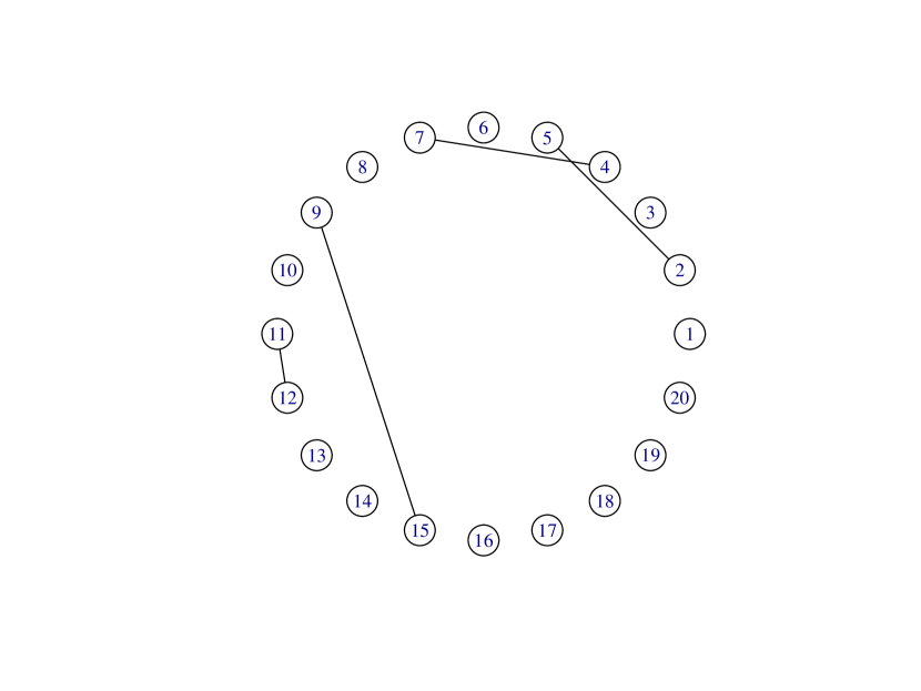
$k=1$

$k=4$

$k=9$

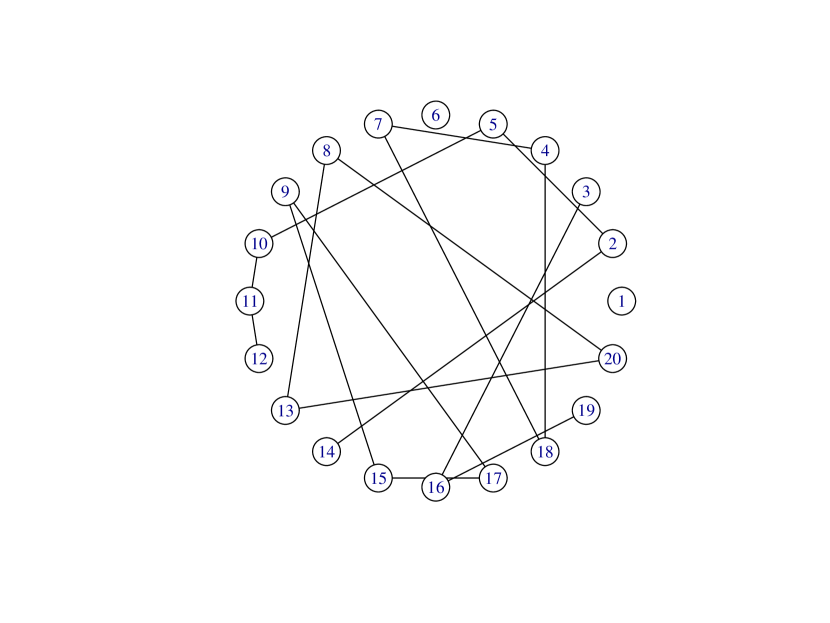
$k=12$

$k=16$

Figure 1: True graph and sequence of successive updates of $\widehat{\mathcal{A}}_{j}^{k}$, for $k=1,4,9,12,16$ of the GSA.

3 Numerical results and real data example

We conducted extensive Monte Carlo simulations to investigate the performance of GS. In this section we report some results from this study and a numerical experiment using real data.

3.1 Monte Carlo simulation study

Simulated Models

We consider three dimension values $p=50,100,150$ and three different models for $\boldsymbol{\Omega}$:

• Model 1. Autoregressive model of orden $1$, denoted $\text{AR}(1)$. In this case $\Sigma_{ij}=0.4^{|i-j|}$ for $i,j=1,\ldots p$.

• Model 2. Nearest neighbors model of order 2, denoted $\text{NN}(2)$. For each node we randomly select two neighbors and choose a pair of symmetric entries of $\boldsymbol{\Omega}$ using the NeighborOmega function of the R package Tlasso.

• Model 3. Block diagonal matrix model with $q$ blocks of size $p/q$, denoted BG. For $p=50,100$ and $150$, we use $q=10,20$ and $30$ blocks, respectively. Each block, of size $p/q=5$, has diagonal elements equal to $1$ and off-diagonal elements equal to $0.5$.

For each $p$ and each model we generate $R=50$ random samples of size $n=100$. These graph models are widely used in the genetic literature to model gene expression data. See for example Lee and Liu (2015) and Lee and Ghi (2006). Figure 2 displays graphs from Models 1-3 with $p=100$ nodes.

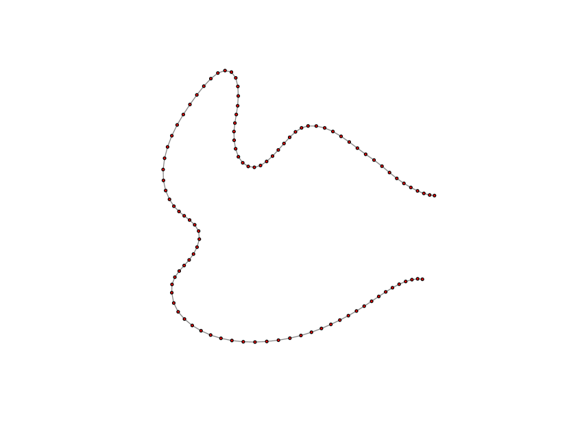
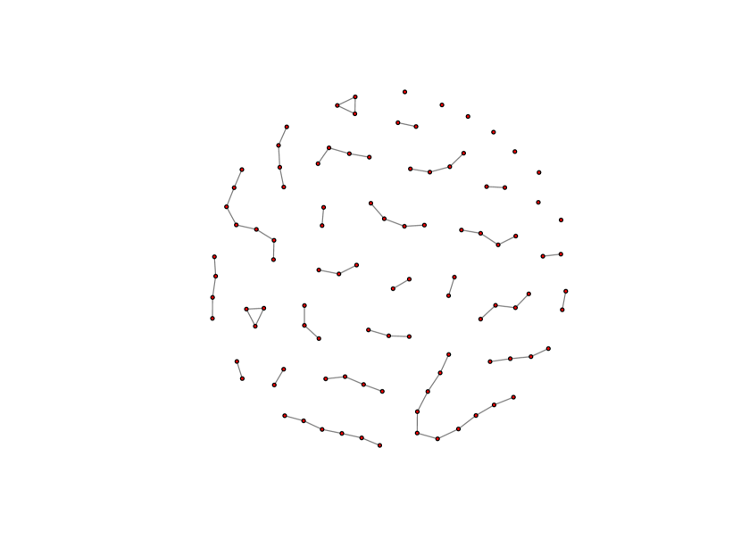
$\text{AR}(1)$

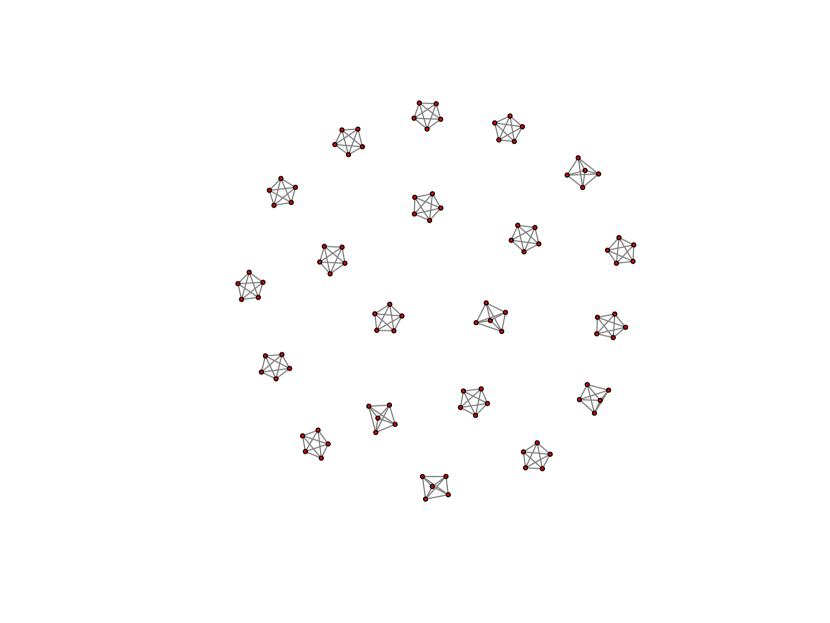
$\text{NN}(2)$

BG

Figure 2: Graphs of $\text{AR}(1)$, $\text{NN}(2)$ and BG graphical models for $p=100$ nodes.

Methods

We compare the performance of GS with Graphical lasso (Glasso) and Constrained $l_{1}$-minimization for inverse matrix estimation (CLIME) proposed by Friedman et al. (2008) and Cai et al. (2011) respectively. Therefore, the methods compared in our simulation study are:

• The proposed method GS with the forward and backward thresholds, $\left({\alpha}_{f},{\alpha}_{b}\right)$, estimated by $5$-fold crossvalidation on a grid of $20$ values in $[0,1]\times[0,1]$, as described in Subsection 2.4. The computing algorithm is available by request.

• The Glasso estimate obtained by solving the $\ell_{1}$ penalized-likelihood problem:

  $$\min_{\boldsymbol{\Omega}\succ 0}\ \left(-\text{log}\{\text{det}[\boldsymbol{\Omega}]\}+\text{tr}\{\boldsymbol{\Omega}\textbf{X}^{\top}\textbf{X}\}+\lambda\parallel\boldsymbol{\Omega}\parallel_{1}\right).$$ (3.1)

  In our simulations and examples we use the R-package CVglasso with the tuning parameter $\lambda$ selected by $5-$fold crossvalidation (the package default).

• The CLIME estimate obtained by symmetrization of the solution of

  $$\min\{\parallel\boldsymbol{\Omega}\parallel_{1}\text{ subject to }\left|S\boldsymbol{\Omega}-\boldsymbol{I}\right|_{\infty}\leq\lambda\},$$ (3.2)

  where $S$ is the sample covariance, $\boldsymbol{I}$ is the identity matrix, $\left|\cdot\right|_{\infty}$ is the elementwise $l_{\infty}$ norm, and $\lambda$ is a tuning parameter. For computations, we use the R-package clime with the tuning parameter $\lambda$ selected by $5-$fold crossvalidation (the package default).

To evaluate the ability of the methods for finding the pairs of edges, for each replicate, we compute the Matthews correlation coefficient (Matthews, 1975)

$$\text{MCC}=\frac{\text{TP}\times\text{TN}-\text{FP}\times\text{FN}}{\sqrt{(\text{TP}+\text{FP})(\text{TP}+\text{FN})(\text{TN}+\text{FP})(\text{TN}+\text{FN})}},$$ (3.3)

the $\text{Specificity}=\text{TN}/(\text{TN}+\text{FP})$ and the $\text{Sensitivity}=\text{TP}/(\text{TP}+\text{FN})$, where TP, TN, FP and FN are, in this order, the number of true positives, true negatives, false positives and false negatives, regarding the identification of the nonzero off-diagonal elements of $\boldsymbol{\Omega}$. Larger values of MCC, Sensitivity and Specificity indicate a better performance (Fan et al., 2009; Baldi et al., 2000).

For every replicate, the performance of $\widehat{\boldsymbol{\Omega}}$ as an estimate for ${\boldsymbol{\Omega}}$ is measured by $m_{F}=||\widehat{\boldsymbol{\Omega}}-\boldsymbol{\Omega}||_{F}$ (where $||\cdot||_{F}$ denotes the Frobenius norm) and by the normalized Kullback-Leibler divergence defined by $m_{NKL}=D_{KL}/(1+D_{KL})$ where

$$D_{KL}=\frac{1}{2}\left(\text{tr}\left\{\widehat{\boldsymbol{\Omega}}\boldsymbol{\Omega}^{-1}\right\}-\text{log}\left\{\text{det}\left[\widehat{\boldsymbol{\Omega}}\boldsymbol{\Omega}^{-1}\right]\right\}-p\right)$$

is the the Kullback-Leibler divergence between $\widehat{\boldsymbol{\Omega}}$ and $\boldsymbol{\Omega}$.

Results

Table 1 shows the MCC performance for the three methods under Models 1-3. GS clearly outperforms the other two methods while CLIME just slightly outperforms Glasso. Cai et al. (2011) pointed out that a procedure yielding a more sparse $\widehat{\boldsymbol{\Omega}}$ is preferable because this facilitates interpretation of the data. The sensitivity and specificity results, reported in Table 4 in Appendix, show that in general GS is more sparse than the CLIME and Glasso, yielding fewer false positives (more specificity) but a few more false negatives (less sensitivity). Table 2 shows that under models $\text{AR}(1)$ and $\text{NN}(2)$ the three methods achieve fairly similar performances for estimating $\Omega$. However, under model BG, GS clearly outperforms the other two.

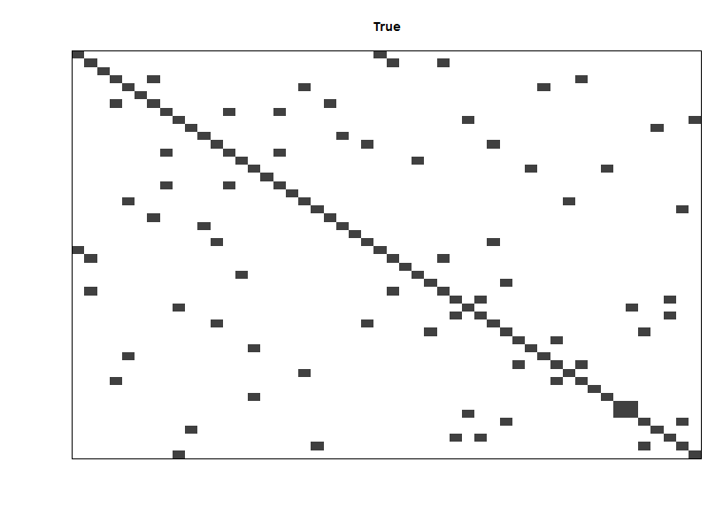
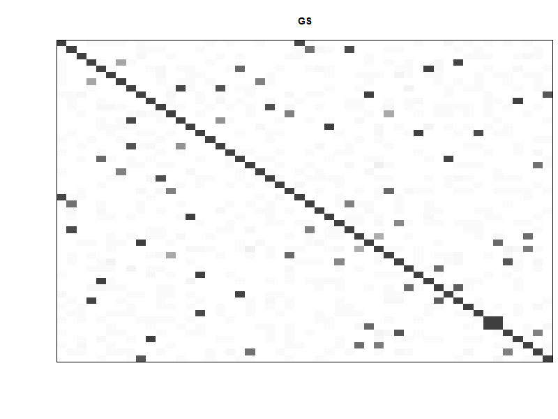
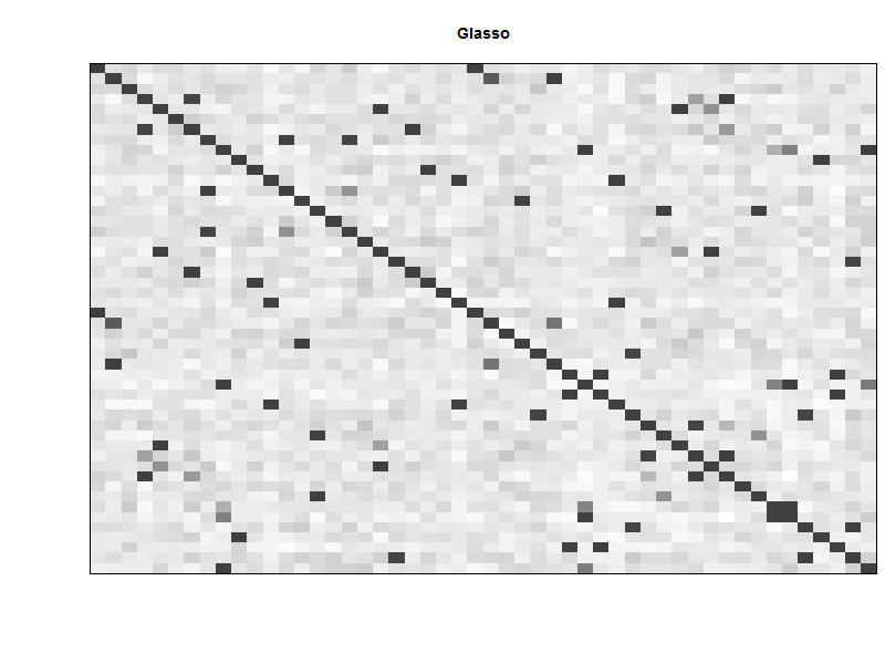
(a) $p=50$

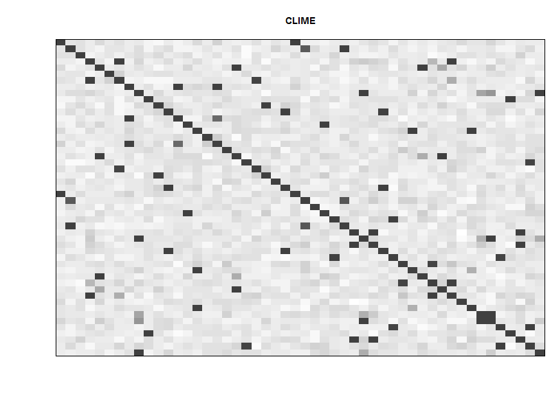
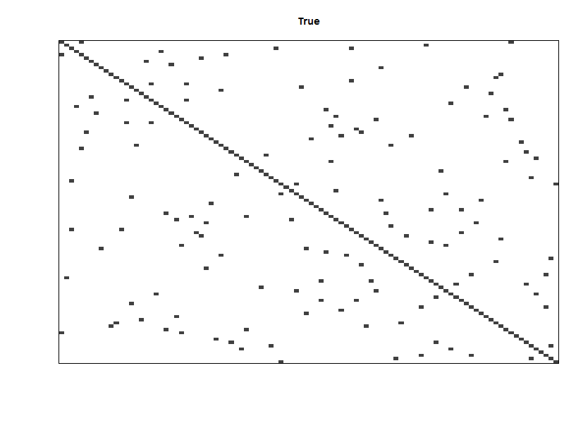
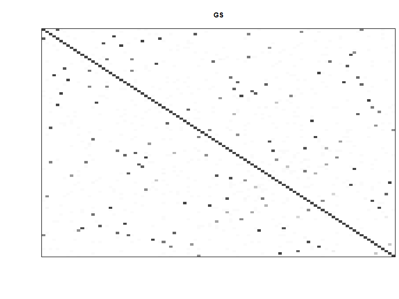
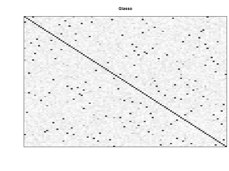
(b) $p=100$

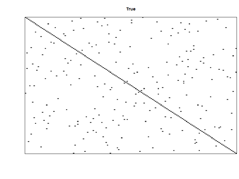
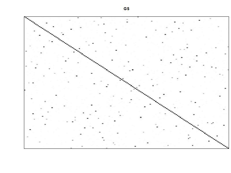
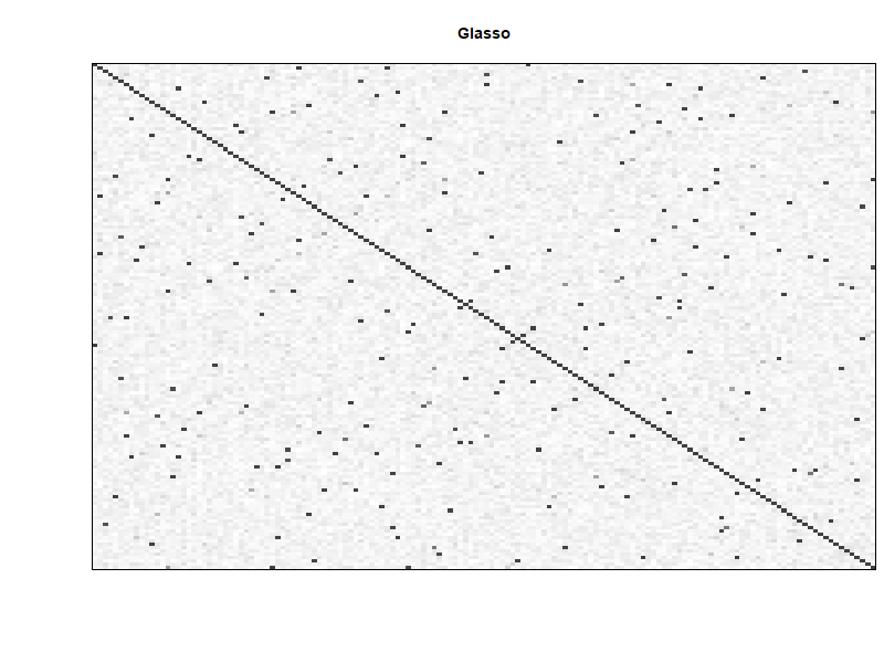
(c) $p=150$

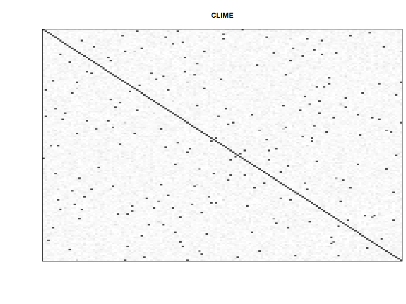
Figure 4: Model $\text{NN}(2)$. Heatmaps of the frequency of the zeros identified for each entry of the precision matrix out of $R=50$ replications. White color is 50 zeros identified out of 50 runs, and black is 0/50.

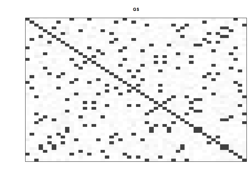
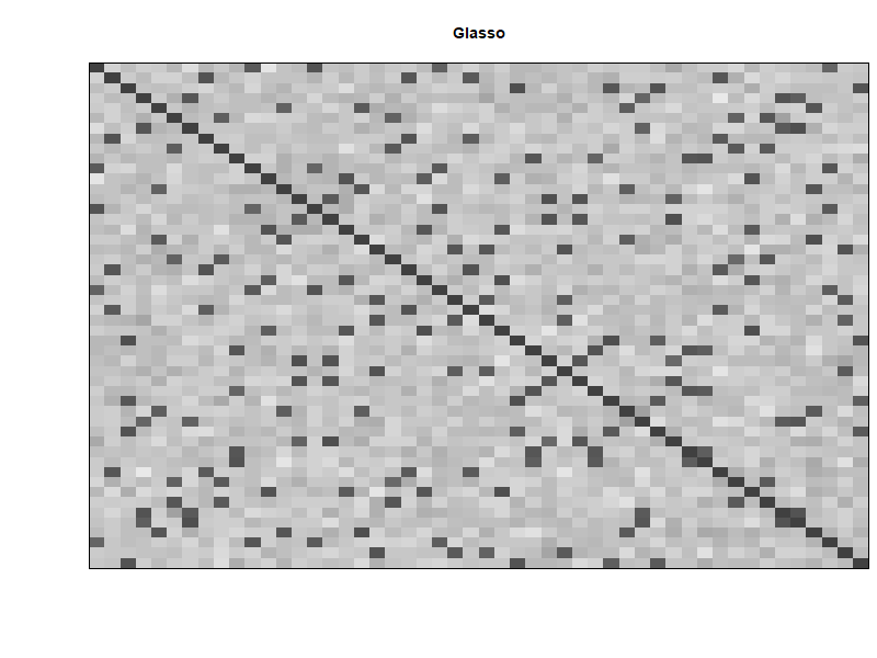
(a) $p=50$

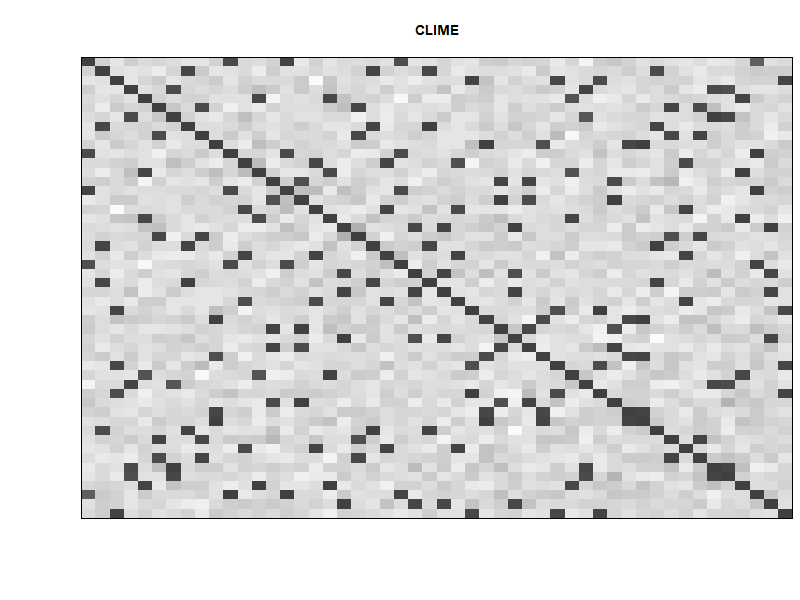
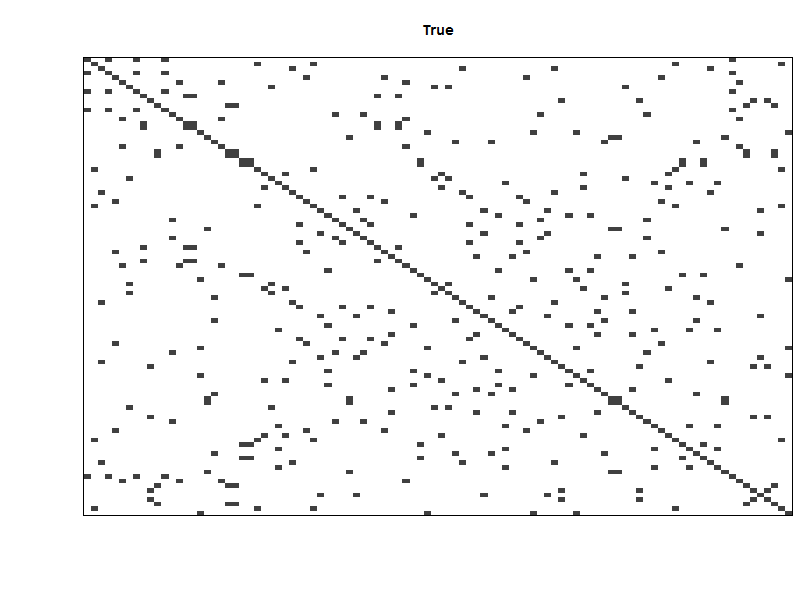
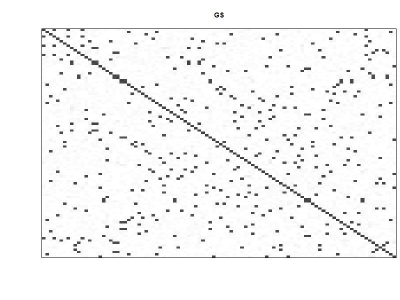
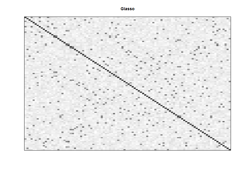
(b) $p=100$

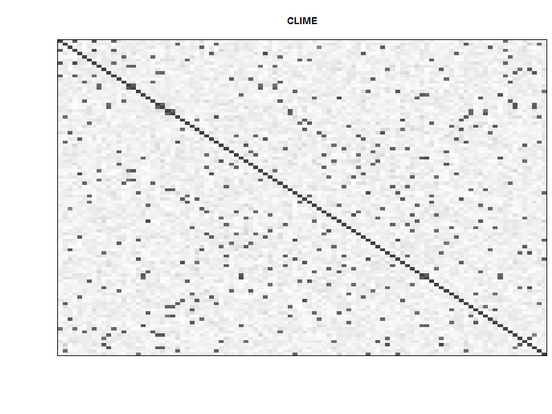
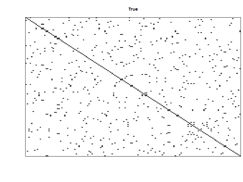
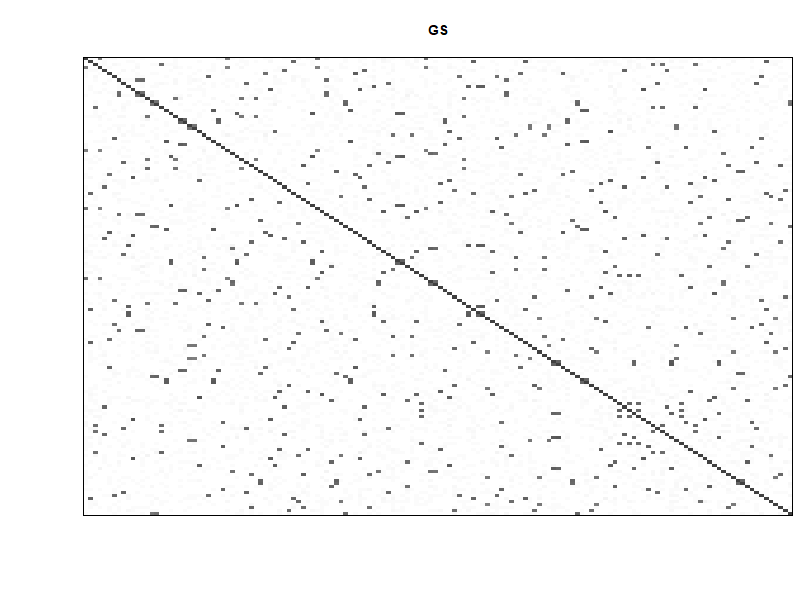
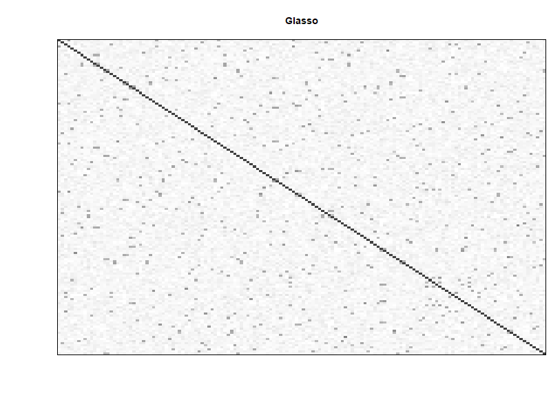
(c) $p=150$

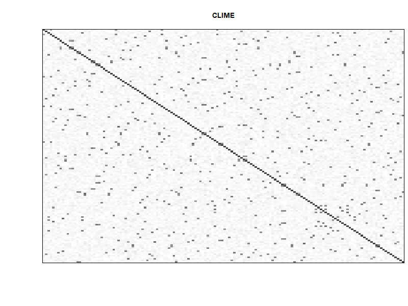
Figure 5: Model BG. Heatmaps of the frequency of the zeros identified for each entry of the precision matrix out of $R=50$ replications. White color is 50 zeros videntified out of 50 runs, and black is 0/50.

Figure 3 display the heat-maps of the number of non-zero links identified in the $50$ replications under model $\text{AR}(1)$. Notice that among the three compared methods, the GS sparsity patterns best match those of the true model. Figures 4 and 5 in the Appendix lead to similar conclusions for models $\text{NN}(2)$ and BG.

Table 1: Comparison of means and standard deviations (in brackets) of MCC over $R=50$ replicates.

Model	$p$	GS	Glasso	CLIME
	50	0.741 (0.009)	0.419 (0.016)	0.492 (0.006)
$\text{AR}(1)$	100	0.751 (0.004)	0.433 (0.020)	0.464 (0.004)
	150	0.730 (0.004)	0.474 (0.017)	0.499 (0.003)
	50	0.751 (0.004)	0.404 (0.014)	0.401 (0.007)
$\text{NN}(2)$	100	0.802 (0.005)	0.382 (0.006)	0.407 (0.005)
	150	0.695 (0.007)	0.337 (0.008)	0.425 (0.003)
	50	0.898 (0.005)	0.356 (0.009)	0.482 (0.005)
BG	100	0.857 (0.005)	0.348 (0.004)	0.461 (0.002)
	150	0.780 (0.008)	0.314 (0.003)	0.408 (0.003)

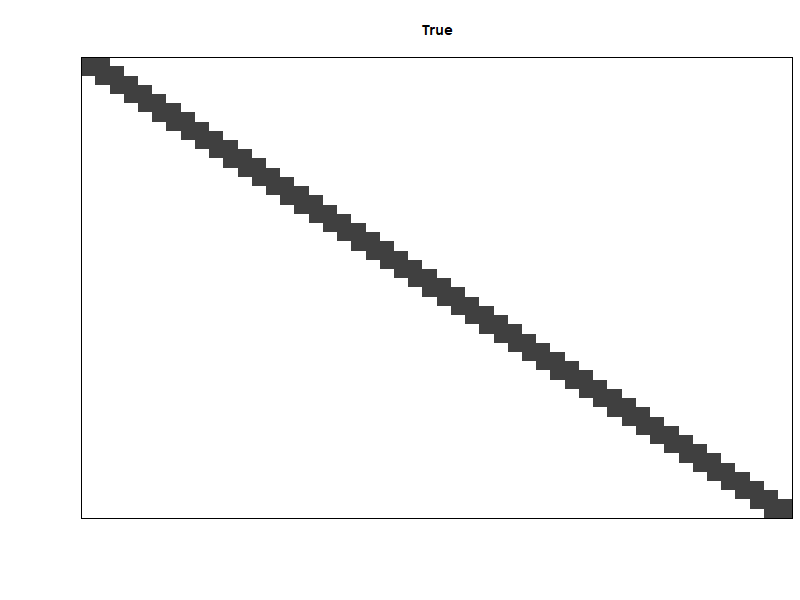
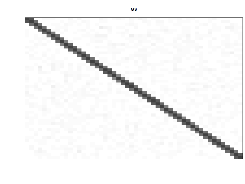
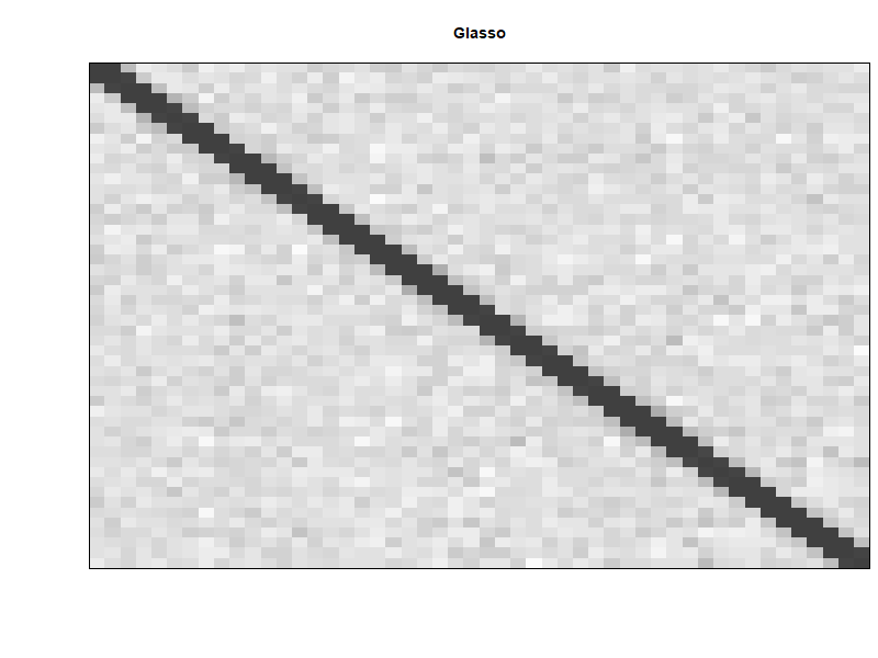
(a) $p=50$

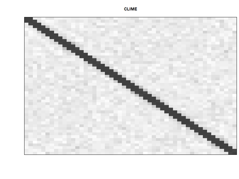
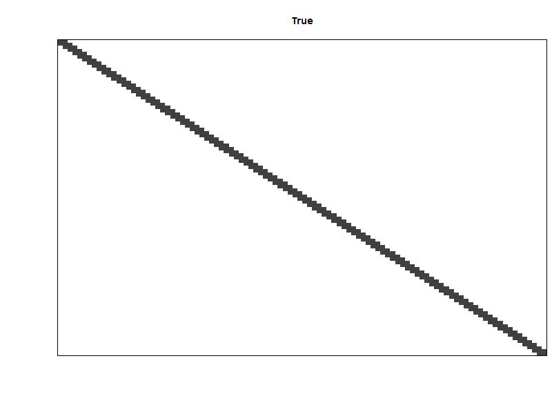
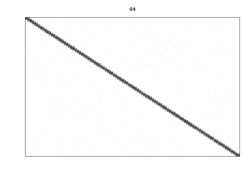
(b) $p=100$

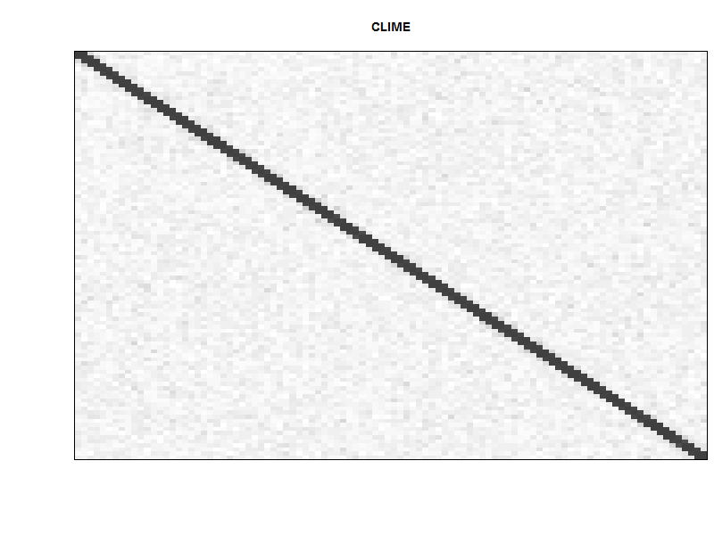
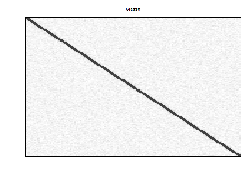
(c) $p=150$

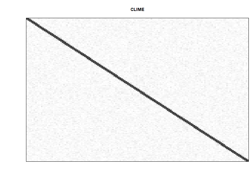
Figure 3: Model $\text{AR}(1)$. Heatmaps of the frequency of the zeros identified for each entry of the precision matrix out of $R=50$ replicates. White color is 50 zeros identified out of 50 runs, and black is 0/50.

Table 2: Comparison of means and standard deviations (in brackets) of $\text{m}_{F}$ and $\text{m}_{NKL}$ over $R=50$ replicates.

		GS		Glasso		CLIME
Model	$p$	$\text{m}_{NKL}$	$\text{m}_{F}$	$\text{m}_{NKL}$	$\text{m}_{F}$	$\text{m}_{NKL}$	$\text{m}_{F}$
	50	0.70	3.82	0.64	3.90	0.63	3.91
		(0.00)	(0.00)	(0.00)	( 0.02)	(0.00)	(0.01)
$\text{AR}(1)$	100	0.83	5.73	0.80	5.72	0.79	5.75
		(0.00)	(0.00)	(0.00)	(0.02)	(0.00)	(0.01)
	150	1.25	7.16	1.17	7.21	1.17	7.25
		(0.00)	(0.00)	(0.00)	(0.02)	(0.00)	(0.01)
	50	0.99	6.98	0.99	6.65	0.99	6.64
		(0.00)	(0.00)	(0.00)	(0.01)	(0.00)	(0.00)
$\text{NN}(2)$	100	0.10	10.11	1.00	9.64	1.00	9.601
		(0.00)	(0.00)	(0.00)	(0.009)	(0.000)	(0.005)
	150	1.00	12.37	1.00	11.90	1.00	11.79
		(0.00)	(0.00)	(0.00)	(0.01)	(0.00)	(0.00)
BG	50	0.46	1.44	0.85	5.45	0.82	5.03
		(0.00)	(0.00)	(0.00)	(0.10)	(0.00)	(0.05)
	100	0.71	2.94	0.93	9.16	0.92	8.71
		(0.00)	(0.00)	(0.00)	(0.07)	(0.00)	(0.02)
	150	0.88	6.10	0.96	11.59	0.96	11.42
		(0.00)	(0.00)	(0.00)	(0.06)	(0.00)	(0.02)

3.2 Analysis of Breast Cancer Data

In preoperative chemoterapy, the complete eradication of all invasive cancer cells is referred to as pathological complete response, abbreviated as pCR. It is known in medicine that pCR is associated with the long-term cancer-free survival of a patient. Gene expression profiling (GEP) – the measurement of the activity (expression level) of genes in a patient – could in principle be a useful predictor for the patient’s pCR.

Using normalized gene expression data of patients in stages I-III of breast cancer, Hess et al. (2006) aim to identify patients that may achieve pCR under sequential anthracycline paclitaxel preoperative chemotherapy. When a patient does not achieve pCR state, he is classified in the group of residual disease (RD), indicating that cancer still remains. Their data consist of 22283 gene expression levels for 133 patients, with 34 pCR and 99 RD. Following Fan et al. (2009) and Cai et al. (2011) we randomly split the data into a training set and a testing set. The testing set is formed by randomly selecting 5 pCR patients and 16 RD patients (roughly $1/6$ of the subjects) and the remaining patients form the training set. From the training set, a two sample t-test is performed to select the 50 most significant genes. The data is then standardized using the standard deviation estimated from the training set.

We apply a linear discriminant analysis (LDA) to predict whether a patient may achieve pathological complete response (pCR), based on the estimated inverse covariance matrix of the gene expression levels. We label with $r=1$ the pCR group and $r=2$ the RD group and assume that data are normally distributed, with common covariance matrix $\boldsymbol{\Sigma}$ and different means $\boldsymbol{\mu}_{r}$. From the training set, we obtain $\widehat{\boldsymbol{\mu}}_{r}$, $\widehat{\boldsymbol{\Omega}}$ and for the test data compute the linear discriminant score as follows

$$\delta_{r}(\textbf{x})=\textbf{x}^{\top}\widehat{\boldsymbol{\Omega}}\widehat{\boldsymbol{\mu}}_{r}-\frac{1}{2}\boldsymbol{\mu}_{r}^{\top}\widehat{\boldsymbol{\Omega}}\boldsymbol{\mu}_{r}+\text{log}\widehat{\pi}_{r}\quad\text{for}\;i=1,\ldots,n,$$ (3.4)

where $\widehat{\pi}_{r}$ is the proportion of group $r$ subjects in the training set. The classification rule is

$$\widehat{r}(\textbf{x})=\operatorname*{argmax}\delta_{r}(\textbf{x})\;\;\;\text{for}\;r=1,2.$$ (3.5)

For every method we use 5-fold cross validation on the training data to select the tuning constants. We repeat this scheme 100 times.

Table 3 displays the means and standard errors (in brackets) of Sensitivity, Specificity, MCC and Number of selected Edges using $\widehat{\boldsymbol{\Omega}}$ over the 100 replications. Considering the MCC, GS is slightly better than CLIME and CLIME than Glasso. While the three methods give similar performance considering the Specificity, GS and CLIME improve over Glasso in terms of Sensitivity.

Table 3: Comparison of means and standard deviations (in brackets) of Sensitivity, Specificity, MCC and Number of selected edges over 100 replications.

	GS	CLIME	Glasso
Sensitivity	0.798 (0.02)	0.786 (0.02)	0.602 (0.02)
Specificity	0.784 (0.01)	0.788 (0.01)	0.767 (0.01)
MCC	0.520 (0.02)	0.516 (0.02)	0.334 (0.02)
Number of Edges	54 (2)	4823 (8)	2103 (76)

4 Concluding remarks

This paper introduces a stepwise procedure, called GS, to perform covariance selection in high dimensional Gaussian graphical models. Our method uses a different parametrization of the Gaussian graphical model based on Pearson correlations between the best-linear-predictors prediction errors. The GS algorithm begins with a family of empty neighborhoods and using basic steps, forward and backward, adds or delete edges until appropriate thresholds for each step are reached. These thresholds are automatically determined by cross–validation.

GS is compared with Glasso and CLIME under different Gaussian graphical models ($\text{AR}(1)$, $\text{NN}(2)$ and BG) and using different performance measures regarding network recovery and sparse estimation of the precision matrix $\Omega$. GS is shown to have good support recovery performance and to produce simpler models than the other two methods (i.e. GS is a parsimonious estimation procedure).

We use GS for the analysis of breast cancer data and show that this method may be a useful tool for applications in medicine and other fields.

Appendix A Appendix

A.1 Selection of the thresholds parameters by cross-validation

Let $\boldsymbol{X}$ be the $n\times p$ matrix with rows $\mathbf{x}_{i}=\left(x_{i1},\ldots,x_{ip}\right)$, $i=1,\ldots,n$, corresponding to $n$ observations. For each $j=1,\ldots,p$, let $\mathbf{X}_{j}=\left(x_{1j},\ldots,x_{nj}\right)^{\top}$ denote the jth–column of the matrix $\mathbf{X}$.

We randomly partition the dataset $\{\mathbf{x}_{i}\}_{1\leq i\leq n}$ into $K$ disjoint subsets of approximately equal size, the $t^{th}$ subset being of size $n_{t}\geq 2$ and $\displaystyle\sum_{t=1}^{K}n_{t}=n$. For every $t$, let $\displaystyle\{\mathbf{x}_{i}^{(t)}\}_{1\leq i\leq n_{t}}$ be the $t^{th}$ validation subset, and its complement $\displaystyle\{\widetilde{\mathbf{x}}_{i}^{(t)}\}_{1\leq i\leq n-n_{t}}$, the $t^{th}$ training subset.

For every $t=1,\ldots,K$ and threshold parameters $(\alpha_{f},\alpha_{b})\in[0,1]\times[0,1]$ let $\widehat{\mathcal{A}}_{1}^{(t)},\ldots,\widehat{\mathcal{A}}_{p}^{(t)}$ be the estimated neighborhoods given by GSA using the $t^{th}$ training subset $\displaystyle\{\widetilde{\mathbf{x}}_{i}^{(t)}\}_{1\leq i\leq n-n_{t}}$ with $\widetilde{\mathbf{x}}_{i}^{(t)}=(\widetilde{x}_{i1}^{(t)},\ldots,\widetilde{x}_{ip}^{(t)}),$ $1\leq i\leq n-n_{t}$. Consider for every node $j$ the estimated neighborhood $\widehat{\mathcal{A}}^{(t)}_{j}=\left\{l_{1},\ldots,l_{q}\right\}$ and let $\widehat{\beta}_{\widehat{\mathcal{A}}_{j}^{(t)}}$ be the estimated coefficient of the regression of $\widetilde{\mathbf{X}}_{j}=(\widetilde{x}_{1j}^{(t)},\ldots,\widetilde{x}_{n-n_{t}j}^{(t)})^{\top}$ on $X_{l_{1}},\ldots,X_{l_{q}}$, represented in (A.10) (red colour).

Consider the $t^{th}$ validation subset $\displaystyle\{\mathbf{x}_{i}^{(t)}\}_{1\leq i\leq n_{t}}$ with $\mathbf{x}_{i}^{(t)}=(x_{i1}^{(t)},\ldots,x_{ip}^{(t)})$, $1\leq i\leq n_{t}$ and for every $j$ let $\mathbf{X}_{j}^{(t)}=\left(x_{1j}^{(t)},\ldots,x_{n_{t}j}^{(t)}\right)^{\top}$ and define the vector of predicted values

$$\widehat{\mathbf{X}}_{j}^{(t)}\left(\alpha_{f},\alpha_{b}\right)=\mathbf{X}_{\widehat{\mathcal{A}}_{j}^{(t)}}\widehat{\beta}_{\mathcal{A}_{j}^{(t)}}^{(t)},$$

where $\mathbf{X}_{\widehat{\mathcal{A}}_{j}^{(t)}}$ is the matrix with rows $(x_{il_{1}}^{(t)},\ldots,x_{il_{q}}^{(t)})$, $1\leq i\leq n_{t}$ represented in (A.10) (in blue colour). If the neighborhood $\mathcal{A}_{j}^{(t)}=\emptyset$ we define

$$\widehat{\mathbf{X}}_{j}^{(t)}\left(\alpha_{f},\alpha_{b}\right)=(\bar{x}_{j}^{(t)},\ldots,\bar{x}_{j}^{(t)})^{\top}$$

where $\bar{x}_{j}^{(t)}$ is the mean of the sample of observations $x_{1j}^{(t)},\ldots,x_{n_{t}j}^{(t)}$.

We define the $K$–fold cross–validation function as

$$CV\left(\alpha_{f},\alpha_{b}\right)=\frac{1}{n}\sum_{t=1}^{K}\sum_{j=1}^{p}\left\|\mathbf{X}_{j}^{(t)}-\widehat{\mathbf{X}}_{j}^{(t)}\left(\alpha_{f},\alpha_{b}\right)\right\|^{2}$$

where $\left\|\cdot\right\|$ the L2-norm or euclidean distance in $\mathbb{R}^{p}$. Hence the $K$–fold cross–validation forward–backward thresholds $\widehat{\alpha}_{f}$, $\widehat{\alpha}_{b}$ is

$$\left(\widehat{\alpha}_{f},\widehat{\alpha}_{b}\right)=:\mathop{\rm argmin}_{\left(\alpha_{f},\alpha_{b}\right)\in\mathcal{H}}CV\left(\alpha_{f},\alpha_{b}\right)$$ (A.1)

where $\mathcal{H}$ is a grid of ordered pairs $\left(\alpha_{f},\alpha_{b}\right)$ in $[0,1]\times[0,1]$ over which we perform the search.

$$\left(\begin{array}[]{c c ccccccccc}t^{th}&\text{training}&\text{subset }\\ \cdots&{\color[rgb]{1,0,0}\widetilde{x}_{1j}^{(t)}}&\cdots&{\color[rgb]{1,0,0}\widetilde{x}_{1l_{1}}^{(t)}}&\cdots&{\color[rgb]{1,0,0}\widetilde{x}_{1l_{q}}^{(t)}}&\cdots\\ \vspace{0.5cm}\vdots&\vdots&\vdots&\vdots&\vdots&\vdots&\vdots\\ \vspace{0.5cm}\par\cdots&{\color[rgb]{1,0,0}\widetilde{x}_{n-n_{t}j}^{(t)}}&\cdots&{\color[rgb]{1,0,0}\widetilde{x}_{n-n_{t}l_{1}}^{(t)}}&\cdots&{\color[rgb]{1,0,0}\widetilde{x}_{n-n_{t}l_{q}}^{(t)}}&\cdots\\ \hline\cr t^{th}&\text{validation}&\text{subset }\\ \cdots&{\color[rgb]{0,0,1}x_{1j}^{(t)}}&\cdots&{\color[rgb]{0,0,1}x_{1l_{1}}^{(t)}}&\cdots&{\color[rgb]{0,0,1}x_{1l_{q}}^{(t)}}&\cdots\\ \vdots&\vdots&\vdots&\vdots&\vdots&\vdots&\vdots\\ \cdots&{\color[rgb]{0,0,1}x_{n_{t}j}^{(t)}}&\cdots&{\color[rgb]{0,0,1}x_{n_{t}l_{1}}^{(t)}}&\cdots&{\color[rgb]{0,0,1}x_{n_{t}l_{q}}^{(t)}}&\cdots\\ \end{array}\right)$$ (A.10)

Remark 3.

Matrix (A.10) represents, for every node $j$ the comparison between estimated and predicted values for cross-validation. $\widehat{\beta}_{\widehat{\mathcal{A}}_{j}^{(t)}}$ is computed using the observations $\widetilde{\mathbf{X}}_{j}=(\widetilde{x}_{1j}^{(t)},\ldots,\widetilde{x}_{n-n_{t}j}^{(t)})^{\top}$ and the matrix $\widetilde{\mathbf{X}}_{\widehat{\mathcal{A}}^{(t)}_{j}}$ with rows $(\widetilde{x}_{il_{1}}^{(t)},\ldots,\widetilde{x}_{il_{q}}^{(t)})$, $i=1,\ldots,n-n_{t}$ in the $t^{th}$ training subset (red colour). Based on the $t^{th}$ validation set $\widehat{\mathbf{X}}_{j}^{(t)}$ is computed using $\mathbf{X}_{\widehat{\mathcal{A}}_{j}^{(t)}}$ and compared with $\mathbf{X}_{j}$ (in blue color).

A.2 Complementary simulation results

Table 4: Comparison of means and standard deviations (in brackets) of Specificity, Sensitivity and MCC over $R=50$ replicates.

		GS			Glasso			CLIME
Model	$p$	Sensitivity	Specificity	MCC	Sensitivity	Specificity	MCC	Sensitivity	Specificity	MCC
	50	0.756	0.988	0.741	0.994	0.823	0.419	0.988	0.891	0.492
		(0.015)	(0.002)	(0.009)	(0.002)	(0.012)	(0.016)	(0.002)	(0.003)	(0.006)
$\text{AR}(1)$	100	0.632	0.999	0.751	0.989	0.897	0.433	0.983	0.934	0.464
		(0.007)	(0.000)	(0.004)	(0.002)	(0.009)	(0.020)	(0.002)	(0.001)	(0.004)
	150	0.607	0.999	0.730	0.981	0.943	0.474	0.972	0.964	0.499
		(0.006)	(0.000)	(0.004)	(0.002)	(0.007)	(0.017)	(0.002)	(0.001)	(0.003)
	50	0.632	0.999	0.751	0.971	0.864	0.404	0.984	0.875	0.401
		(0.007)	(0.000)	(0.004 )	(0.004)	(0.010)	(0.014)	(0.003)	(0.004)	(0.007)
$\text{NN}(2)$	100	0.730	0.999	0.802	0.987	0.924	0.382	0.985	0.937	0.407
		(0.008)	(0.000)	(0.005)	(0.002)	(0.004)	(0.006)	(0.002)	(0.001)	(0.005)
	150	0.555	0.999	0.695	0.952	0.936	0.337	0.934	0.965	0.425
		(0.017)	(0.000)	(0.007)	(0.004)	(0.002)	(0.008)	( 0.003)	(0.001)	(0.003)
	50	0.994	0.981	0.898	0.867	0.697	0.356	0.962	0.807	0.482
		(0.002)	(0.001)	(0.005)	(0.032)	(0.021)	(0.009)	(0.004)	(0.005)	(0.005)
BG	100	0.949	0.989	0.857	0.569	0.908	0.348	0.818	0.920	0.4615
		(0.007)	(0.000)	(0.005)	(0.039)	(0.011)	( 0.004)	(0.005)	(0.005)	(0.002)
	150	0.782	0.994	0.780	0.426	0.952	0.314	0.626	0.959	0.408
		(0.021)	(0.000)	(0.008)	(0.035)	(0.006)	(0.003)	(0.006)	(0.001)	(0.003)

References

- Anderson (2003) Anderson, T. (2003). An Introduction to Multivariate Statistical Analysis. John Wiley.
- Baldi et al. (2000) Baldi, P., S. Brunak, Y. Chauvin, C. Andersen, and H. Nielsen (2000). Assessing the accuracy of prediction algorithms for classification: An overview. Bioinformatics 16(5), 412–424.
- Banerjee et al. (2008) Banerjee, O., L. El Ghaoui, and A. d’Aspremont (2008). Model selection through sparse maximum likelihood estimation for multivariate gaussian or binary data. The Journal of Machine Learning Research 9, 485–516.
- Bühlmann and Van De Geer (2011) Bühlmann, P. and S. Van De Geer (2011). Statistics for high-dimensional data: methods, theory and applications. Springer Science & Business Media.
- Cai et al. (2011) Cai, T., W. Liu, and X. Luo (2011). A constrained minimization approach to sparse precision matrix estimation. Journal of the American Statistical Association 106(494), 594–607.
- Cramér (1999) Cramér, H. (1999). Mathematical Methods of Statistics. Princeton University Press.
- Dempster (1972) Dempster, A. P. (1972). Covariance selection. Biometrics, 157–175.
- Eaton (2007) Eaton, M. L. (2007). Multivariate Statistics : A Vector Space Approach. Institute of Mathematical Statistics.
- Edwards (2000) Edwards, D. (2000). Introduction to Graphical Modelling. Springer Science & Business Media.
- Fan et al. (2009) Fan, J., Y. Feng, and Y. Wu (2009). Network exploration via the adaptive lasso and scad penalties. The Annals of Applied Statistics 3(2), 521–541.
- Friedman et al. (2008) Friedman, J., T. Hastie, and R. Tibshirani (2008). Sparse inverse covariance estimation with the graphical lasso. Biostatistics 9(3), 432–441.
- Hess et al. (2006) Hess, K. R., K. Anderson, W. F. Symmans, V. Valero, N. Ibrahim, J. A. Mejia, D. Booser, R. L. Theriault, A. U. Buzdar, P. J. Dempsey, et al. (2006). Pharmacogenomic predictor of sensitivity to preoperative chemotherapy with paclitaxel and fluorouracil, doxorubicin, and cyclophosphamide in breast cancer. Journal of Clinical Oncology 24(26), 4236–4244.
- Huang et al. (2016) Huang, S., J. Jin, and Z. Yao (2016). Partial correlation screening for estimating large precision matrices, with applications to classification. The Annals of Statistics 44(5), 2018–2057.
- Johnson et al. (2011) Johnson, C. C., A. Jalali, and P. Ravikumar (2011). High-dimensional sparse inverse covariance estimation using greedy methods. arXiv preprint arXiv:1112.6411.
- Kalisch and Bühlmann (2007) Kalisch, M. and P. Bühlmann (2007). Estimating high-dimensional directed acyclic graphs with the pc-algorithm. The Journal of Machine Learning Research 8, 613–636.
- Lauritzen (1996) Lauritzen, S. L. (1996). Graphical Models. Oxford University Press.
- Lawrance (1976) Lawrance, A. J. (1976). On conditional and partial correlation. The American Statistician 30(3), 146–149.
- Ledoit and Wolf (2004) Ledoit, O. and M. Wolf (2004). A well-conditioned estimator for large-dimensional covariance matrices. Journal of Multivariate Analysis 88(2), 365–411.
- Lee and Ghi (2006) Lee, H. and J. Ghi (2006). Gradient directed regularization for sparse gaussian concentration graphs, with applications to inference of genetic networks. Biostatistics 7(2), 302–317.
- Lee and Liu (2015) Lee, W. and Y. Liu (2015). Joint estimation of multiple precision matrices with common structures. Journal of Machine Learning Research 16(1), 1035−1062.
- Liang et al. (2015) Liang, F., Q. Song, and P. Qiu (2015). An equivalent measure of partial correlation coefficients for high-dimensional gaussian graphical models. Journal of the American Statistical Association 110(511), 1248–1265.
- Liu and Wang (2012) Liu, H. and L. Wang (2012). Tiger: A tuning-insensitive approach for optimally estimating gaussian graphical models. arXiv preprint arXiv:1209.2437.
- Matthews (1975) Matthews, B. (1975). Comparison of the predicted and observed secondary structure of t4 phage lysozyme. Biochimica et Biophysica Acta 405(2), 442−451.
- Meinshausen and Bühlmann (2006) Meinshausen, N. and P. Bühlmann (2006). High-dimensional graphs and variable selection with the lasso. The Annals of Statistics 34(3), 1436–1462.
- Peng et al. (2009) Peng, J., P. Wang, N. Zhou, and J. Zhu (2009). Partial correlation estimation by joint sparse regression models. Journal of the American Statistical Association 104(486), 735–746.
- Ravikumar et al. (2011) Ravikumar, P., M. J. Wainwright, G. Raskutti, B. Yu, et al. (2011). High-dimensional covariance estimation by minimizing -penalized log-determinant divergence. Electronic Journal of Statistics 5, 935–980.
- Ren et al. (2015) Ren, Z., T. Sun, C.-H. Zhang, H. H. Zhou, et al. (2015). Asymptotic normality and optimalities in estimation of large gaussian graphical models. The Annals of Statistics 43(3), 991–1026.
- Rütimann et al. (2009) Rütimann, P., P. Bühlmann, et al. (2009). High dimensional sparse covariance estimation via directed acyclic graphs. Electronic Journal of Statistics 3, 1133–1160.
- Spirtes et al. (2000) Spirtes, P., C. N. Glymour, and R. Scheines (2000). Causation, Prediction, and Search. MIT press.
- Yuan (2010) Yuan, M. (2010). High dimensional inverse covariance matrix estimation via linear programming. The Journal of Machine Learning Research 11, 2261–2286.
- Yuan and Lin (2007) Yuan, M. and Y. Lin (2007). Model selection and estimation in the gaussian graphical model. Biometrika 94(1), 19–35.
- Zhou et al. (2011) Zhou, S., P. Rütimann, M. Xu, and P. Bühlmann (2011). High-dimensional covariance estimation based on gaussian graphical models. The Journal of Machine Learning Research 12, 2975–3026.