Large Covariance Matrices: Accurate Models Without Mocks
Abstract
Covariance matrix estimation is a persistent challenge for cosmology. We focus on a class of model covariance matrices that can be generated with high accuracy and precision, using a tiny fraction of the computational resources that would be required to achieve comparably precise covariance matrices using mock catalogues. In previous work, the free parameters in these models were determined using sample covariance matrices computed using a large number of mocks, but we demonstrate that those parameters can be estimated consistently and with good precision by applying jackknife methods to a single survey volume. This enables model covariance matrices that are calibrated from data alone, with no reference to mocks.
1 Introduction
No matter the scope of a cosmological survey, we have only one sky to observe. This complicates the statistical analysis of cosmological surveys. A common approach is to generate a large number of independent, synthetic skies, then apply standard sample statistics to them. The readily apparent limitations of this approach are that it is challenging to ensure that the synthetic skies reflect the physics of the actual universe, and that the computational cost of generating these “mock catalogues” can be substantial. In this paper we take an approach introduced in O’Connell et al. (2016), which generates the covariance matrix for a galaxy correlation function with correct long-distance physics and survey geometry, and extend it so that the short-distance physics can be calibrated directly against a survey, without reference to mocks.
Using mock catalogues to generate a covariance matrix requires a large number of reasonably accurate mocks. The consequences of having an insufficient number of mocks have received significant attention. If mocks are used to generate a covariance matrix for a correlation function estimated using different bins the scale for noise in the covariance matrix is set by . Noise in the covariance matrix propagates through to become additional noise on cosmological parameter estimates, increasing the parameter covariance by a factor of (Dodelson & Schneider, 2013; Percival et al., 2014). We note that the next generation of surveys, including Euclid (Laureijs et al., 2011), DESI (Levi et al., 2013), and WFIRST (Doré et al., 2018) aim at tomographic analyses and that a simultaneous analysis of multiple redshift bins will dramatically increase the number of correlation function bins used.
In O’Connell et al. (2016) we developed a method built on the observation, due to Bernstein (Bernstein, 1994), that the covariance matrix of a 2-point correlation function can itself by written in terms of correlations between four points, integrated over the survey volume. We perform these integrals using a realistic 2-point correlation function and accurately representation of the survey geometry, to produce a covariance matrix that accurately reflects the long-distance physics and structure of the survey. Related work includes Pearson & Samushia (2016), which constructed a simple model of the power spectrum covariance matrix, and Grieb et al. (2016), which took a similar approach to that in O’Connell et al. (2016) but on a cubic, uniform survey.
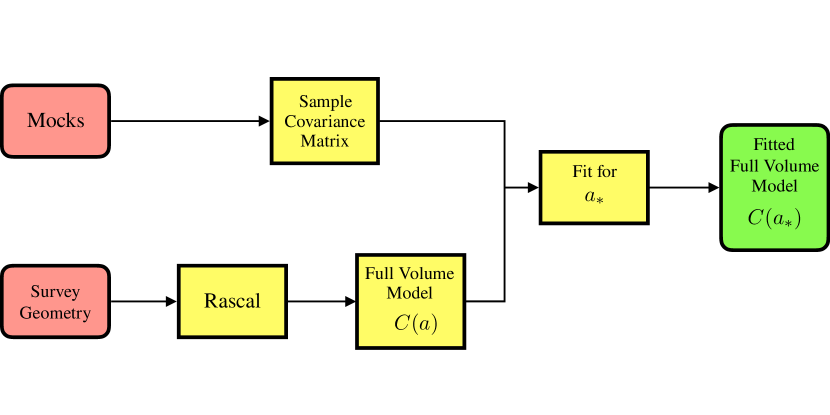
The four-point correlations noted above include contributions from the connected 3- and 4-point galaxy correlation functions, which are not as well-understood as the 2-point function. O’Connell et al. (2016) approximated these contributions by introducing a shot-noise rescaling parameter, , which effectively modelled the short-distance contributions to the covariance matrix from the 3- and 4-point functions as an increase in shot-noise. was estimated using mock catalogues and the resulting fit covariance matrix was found to be both accurate and precise. Critically, this required a tiny fraction of the computational time required to generate a mock covariance matrix of comparable precision. The procedure is illustrated in figure 1. This approach was further tested in Vargas-Magaña et al. (2018), where it was found that the resulting covariance matrix performed at least as well as a mock covariance matrix for BAO measurements with BOSS (Dawson et al., 2013).
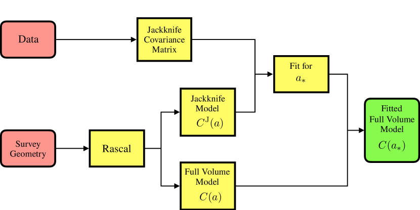
In this paper, we propose to estimate the shot-noise rescaling using actual survey data, rather than mock catalogues. The essential observation is that since is being used to model short-distance physics, we need not use or mimic the entire survey volume in order to estimate it. Instead we propose to use the actual survey to generate a jackknife covariance matrix, then use the jackknife covariance matrix to estimate . The computational cost to do this is quite low, since generating the jackknife covariance matrix requires very little computation beyond counting the pairs in the survey. The estimated value of can then be used in the original model covariance matrix. This new procedure is illustrated in figure 2. We find that the level of precision on that can be achieved with a single survey volume is ample for many applications. It is therefore possible to perform covariance matrix estimation for upcoming surveys without reference to mock catalogues.
The observation that relatively small volumes can provide usable information about the covariance matrix has generated recent interest. Klypin & Prada (2018) investigated the power spectrum covariance matrix using small-volume cubic mocks. Small-volume cubic simulations were also used in Howlett & Percival (2017) to generate a scaled covariance matrix for the 2-point correlation function. The jackknife approach introduced here allows us to utilise small-scale information while accurately reflecting the true survey geometry.
In light of the urgency of the covariance matrix problem for upcoming surveys, many approaches to the problem are currently being developed:
- •
- •
-
•
Several empirical techniques have been developed to smooth sample covariance matrices computed from mocks. These take advantage of resampling methods (Escoffier et al., 2016), shrinkage (Joachimi, 2017), or the sparse structure of the precision matrix (the inverse of the covariance matrix) (Padmanabhan et al., 2016).
The result is that practitioners can combine a variety of physical and statistical insights when analysing a cosmological survey. We hope that our contribution will be useful in this regard.
This paper is organised as follows. In section 2 we briefly review the results of O’Connell et al. (2016), including the full and Gaussian model covariance matrices and the 1-parameter model for non-Gaussian contributions. In section 3 we specify how we will compute a jackknife covariance matrix from a single survey volume and how we will compute the corresponding jackknife model covariance matrix. In section 4 we use mocks to verify that the values of estimated from single survey volumes, using a jackknife, are consistent with the values that would be estimated from those mocks using a sample covariance. This establishes the consistency of our method and provides evidence for our claim that is modelling short-distance physics. We conclude in section 5. In appendix A we present a jackknife-inspired method for accurately inverting a model covariance matrix. That method is used in this paper and may be of interest to researchers working on model covariance matrices in other contexts.
2 Model Covariance Matrices
Given an estimator for a correlation function, the covariance matrix for that estimator is
| (2.1) |
In practice itself is often estimated by evaluating on a large number of mock catalogues, then computing a sample covariance from the . The idea of a model covariance matrix is to use theoretical insights to produce a more direct estimate of . The primary elements of the model we use are the shot noise (which may vary across the survey) and the 2-point correlation function, both of which are assumed to be well-understood. The benefit of the model covariance approach is that high precision for the covariance matrix is readily attained, while the mock approach requires a significant investment of computational resources to achieve even modest degrees of precision. In Percival et al. (2014) it was shown that insufficient precision in the covariance matrix for the correlation function propagates through to reduce the precision of cosmological measurements performed with the correlation function, so methods to improve the precision of covariance matrices have immediate value for observational cosmologists.
In the model covariance matrix approach a primary challenge is finding an accurate way to approximate non-Gaussian contributions to . These are determined by the 3- and 4-point correlation functions, which in most applications are only partially understood. Many approaches to the non-Gaussian contributions are possible; a simple model was introduced in O’Connell et al. (2016) to approximate these contributions by rescaling the shot noise in the survey by a uniform factor . In this section we briefly review the results of O’Connell et al. (2016), including the full and Gaussian model covariance matrices and the 1-parameter model for non-Gaussian contributions.
2.1 Covariance Matrix from -point Functions
To illustrate the method we consider the 2-point correlation function in a galaxy survey. We begin by breaking the survey into a large number of non-overlapping cells, such that each cell contains either one or zero galaxies. Let be the number of galaxies in cell . We also introduce , the number density of galaxies in cell , and , the weight applied to cell , to account for possible inhomogeneities in the survey. The overdensity in cell is then
| (2.2) |
The estimate of the correlation function in bin is
| (2.3) | ||||
| (2.4) |
where is a binning matrix that is one when the separation between cells and falls in correlation function bin and zero otherwise. In the following we will assume that the binning matrices are symmetric, , as is appropriate when estimating an autocorrelation function.
The covariance matrix for is
| (2.5) | ||||
| (2.6) |
In order to connect this expression to point functions we need to remove contributions to the sum from overlapping cells, e.g. where . Such contributions are readily simplified by the following identity,
| (2.7) |
which we think of as a contraction between two ’s. Performing the required contractions and exploiting the symmetry of the binning matrices , we find
| (2.8) |
The connection to point correlation functions is now straightforward,
| (2.9) |
where is the familiar 2-point correlation function, is the 3-point correlation function, and is the 4-point correlation function. A continuum limit yields the expressions familiar from Bernstein (1994) and O’Connell et al. (2016).
2.2 Modelling Non-Gaussianity
If we look over (2.9), we see that it includes and , which as survey properties are assumed to be readily available. The 2-point function also appears, and in most applications is understood with sufficient accuracy to compute its contribution to . The 3- and 4-point functions and , on the other hand, are often only partially understood. When an accurate version of the 3- and/or 4-point functions is not available we could consider a variety of models for non-Gaussian contributions to . One such model approximates the contributions of the 3- and 4-point functions, which we expect to be most relevant at small separations, as additional shot noise. We do this by splitting up the Gaussian contributions in (2.9) as follows:
| (2.10) | ||||
| (2.11) | ||||
| (2.12) |
We can then implement a uniform increase in the shot noise by a factor by taking . Recall that , so the non-Gaussian model is
| (2.13) |
In O’Connell et al. (2016) it was shown that the unknown parameter can be determined by fitting111An updated discussion of fitting methods can be found in section 4. the model to the sample covariance computed from mock catalogues. The resulting model covariance matrix was found to provide suitable accuracy for BOSS-like surveys. Numerical integration techniques introduced in O’Connell et al. (2016) yield precision that dramatically outstrips what can currently be achieved with mocks and require only very modest computational resources ( CPU hours). This combination of accuracy and precision makes the model covariance matrix approach appealing for future studies of large scale structure and motivates our further development of the method here.
3 Jackknife Methods and Model Covariance Matrices
One of the limitations of the method described in section 2.2 is that it relies on mock catalogues to calibrate the unknown parameter , which in turn ensures the accuracy of the model covariance matrix. While fewer mocks are required to calibrate than are required to generate a precise sample covariance matrix, the potential accuracy of the model covariance matrix is limited in part by the accuracy of the mock catalogues. For example, if the connected 4-point function in the mocks is smaller than the connected 4-point function in the actual survey, we expect this to result in a biased estimate of .
Fortunately any reasonably large survey includes sufficient volume to make multiple estimates of the correlation function, and thus contains information about the statistics of the correlation function. One could consider a variety of techniques to extract this information, but here we will use a simple resampling technique, the jackknife, to make an estimate of from a single survey volume. We speculate that in some cases the estimate for obtained from the actual survey data will be sufficient for analysis, making mock catalogues necessary only for controlling biases in the recovered parameters due to systematic effects. When the survey itself does not yield a sufficiently precise estimate of , we can still make improvements by applying jackknife methods to each mock in turn, then combining the results to get a more precise estimate of than the sample covariance of those mocks would allow.
We emphasise that, from the point of view of computational costs, these improvements in the precision of are essentially free. The jackknife procedure that we will describe requires that the pairs in each survey volume be counted only once, and the only change in computational requirements, relative to standard pair-counting, is that separate counts are maintained for each jackknife region. In other words, the computational time required to use our jackknife procedure to estimate with a single survey volume really is of the time required to estimate using a sample covariance computed from 100 mocks.
3.1 The Restricted Jackknife
In the cosmological version of the jackknife a survey is split into regions, then the analysis is repeated times, with a different region left out of the analysis each time. The results can then be combined to provide an estimate of uncertainties associated with the analysis. There are several issues that make cosmological jackknives more complicated to analyse than the traditional statistical jackknife:
-
1.
In analyses that utilise pair counts, some pairs will straddle two jackknife regions.
-
2.
The regions will generally have different shapes and/or areas.
-
3.
Different regions of a cosmological survey are not statistically independent of one another, as is assumed for the traditional jackknife.
Each of these issues will be relevant in our analysis.
For the “restricted” jackknife, we will simply exclude any pairs that straddle two jackknife regions. We choose this for the sake of simplicity and anticipate that a jackknife with a more careful treatment of those pairs could be used without difficulty. The estimate of the correlation function in a single region is
| (3.1) | ||||
| (3.2) |
Jackknife regions are specified by , with if cell is in jackknife region , and otherwise.
We do not assume that the jackknife regions all have the same volume. This is done for two reasons. First, a greater variety of methods for generating jackknife regions can be used if we do not require that all regions have the same volume. In particular, many simple methods, which are more clearly specified and easily communicated to other researchers, do not lead to regions with the same volume. Second, for analyses of the 2-point correlation function the most appropriate notion of “volume” is , which depends on the bin being considered. While we can imagine adaptive techniques to match jackknife region volumes, it will not in general be possible to match across all regions and for all bins .
To combine the different jackknife regions into a single estimate we introduce the following weights,
| (3.3) | ||||
| (3.4) |
Note that the relative weighting between regions depends on which correlation function bin we consider. The analogue of the full correlation function in this approach is a weighted sum of the estimates in each region:
| (3.5) | ||||
| (3.6) | ||||
| (3.7) | ||||
| (3.8) |
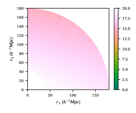
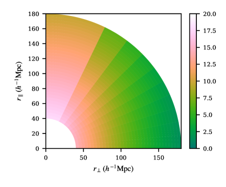
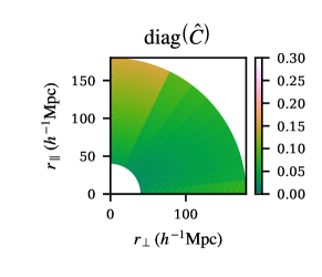
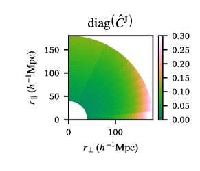
Note that if cells and fall in the same jackknife region and that otherwise. We emphasise that is not equivalent to , as the inclusion of means that pairs that straddle two jackknife regions make no contribution to . A simple way to visualise the difference between the two approaches is to plot and , as we have in Figure 3. The geometry of the jackknife regions is described in detail in section 4.2, but for now it is sufficient to note that our choice of jackknife regions cuts off many pairs at large transverse separation, and this is reflected in .
We use the standard formulation of a weighted jackknife covariance:
| (3.9) |
Because can be written as a weighted average of , the usual prescription in terms of dropped regions reduces to a rescaled sample covariance. The standard formulation of the jackknife covariance provides an unbiased estimate of the true covariance when the jackknife regions are independent. Clearly that’s not the case here, but we’ll find that it is still a reasonable choice.
3.2 Model Covariance for the Restricted Jackknife
As noted above, the jackknife covariance and standard covariance “see” quite different survey geometries, and so it would not be appropriate to fit to . For this reason we will compute a new model, , and compare that to . The covariance of is straightforward to compute:
| (3.10) | ||||
| (3.11) |
As in the previous section, we must perform a series of contractions in order to arrive at expressions that can be interpreted in terms of -point functions. The new twist is that we need to be able to contract the ’s:
| (3.12) | ||||
| (3.13) | ||||
| (3.14) | ||||
| (3.15) | ||||
| (3.16) | ||||
| (3.17) | ||||
| (3.18) |
The expression for the covariance of is then
| (3.19) |
In words, sets of four points only contribute if and fall in a single jackknife region, and and also fall in a single jackknife region. Sets of two or three points only contribute if all points are in the same jackknife region.
As with the original model we can identify three Gaussian contributions to the jackknife covariance:
| (3.20) | ||||
| (3.21) | ||||
| (3.22) |
We use (2.13) as our model for non-Gaussianity, i.e. we implement a uniform increase in the shot noise by a factor by taking :
| (3.23) |
Although the Gaussian contributions , , and are different, both qualitatively and quantitatively, from their full-survey counterparts in in (2.10-2.12), the same numerical methods that facilitate rapid integration of , , and can be used on , , and . The restrictions required for the jackknife model have been added to Rascal222https://github.com/rcoconnell/Rascal, the code used in O’Connell et al. (2016).
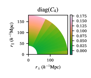
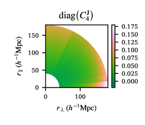
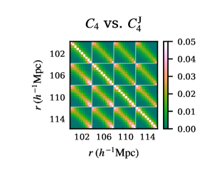
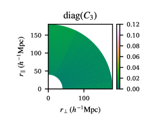
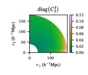
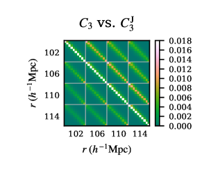
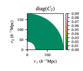
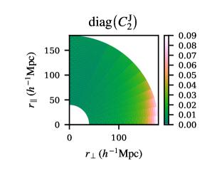
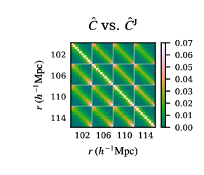
To illustrate the differences between the Gaussian contributions to the model with and without a jackknife, we have plotted each contribution in Figure 4. The jackknife geometry is described in detail in section 4.2, but here we mention that the jackknife regions are defined in angular coordinates and that each jackknife region covers the entire redshift range of the survey. Because the jackknife regions have limited extent in directions transverse to the line-of-sight, the Gaussian contributions with jackknife , , and are dramatically different from the Gaussian contributions without jackknife , , and .
4 Validation with Mocks
The approach we have described assumes that model covariance matrix generation is performed in two steps:
-
1.
Generation of a family of models , using the survey geometry, with a small number of unknown parameters (here one).
-
2.
Estimation of those unknown parameter(s), here .
In previous work (O’Connell et al., 2016) a sample covariance matrix, determined from a large number of mock catalogues, was used to estimate . In this paper we propose to estimate using a jackknife covariance matrix, as described in the previous section. We will consider this new approach valid if it leads to estimates of that are consistent with those that would arise from a sample analysis of a large number of mocks.
To perform this validation we use 1,000 mock catalogues. 900 of these mocks are used to compute a sample covariance and establish a fiducial value for . For each of the 100 remaining mocks we will compute a jackknife covariance matrix, then use that to produce an independent estimate of . We will then demonstrate that the 100 jackknife estimates of are indeed consistent with the fiducial value.
We emphasise that this consistency is a non-trivial result. As shown in Figure 3, the restricted jackknife covariance that we use “sees” less volume, particularly for bins at large transverse separation, than the sample covariance. If the preferred value of the shot-noise rescaling (or other model parameters) were separation-dependent, the resulting difference in weighting between small and large scales for the jackknife versus the sample covariance could lead to inconsistent estimates of . Moreover, we saw in Figure 4 that the jackknife model, , is qualitatively different from the full-volume model, , so without some underlying physical understanding of we might not expect fitting in the two approaches to lead to compatible estimates of .
4.1 Fitting Overview
Following O’Connell et al. (2016), there are two likelihoods we could use for covariance matrix fitting:
| (4.1) | ||||
| (4.2) |
In these expressions and are empirical covariance and precision matrices, estimated from mocks, a jackknife, or by other methods. and are model covariance and precision matrices, computed on the full volume or jackknife geometry, as appropriate. Either likelihood can be minimised to provide an estimate of . While and are distinct likelihoods, we expect them to yield compatible estimates of and the choice of which to use is largely a practical matter. The primary practical consideration in choosing or is our ability to accurately determine or , given or .
When the empirical covariance matrix is computed from independent samples, as is the case with mock catalogues, the estimated matrix follows a Wishart distribution and the inverse follows an inverse-Wishart distribution. Wishart noise means that provides a biased estimate of the true precision matrix, but this bias can be corrected. An unbiased estimate of is provided by:
| (4.3) |
When , as might be the case when the samples in question are individual mock catalogues, it is straightforward to compute , and we might prefer to use for fitting. Unfortunately an unbiased inverse is not available when , and the matrix is singular when . This will be the case in section 4.2, where the samples are jackknife regions and is a jackknife covariance matrix. In such cases we are forced to use , as we will do for the remainder of this section.
In order to use we must invert the model, . This requires some care because is determined by numerical integration, and thus is noisy. In our case the level of noise is very low, but because it is nonzero will provide a biased estimate of . Because the noise on is not Wishart-distributed, the simple correction from (4.3) does not apply. In appendix A we present a partial solution to this problem. The result, which we will use throughout this section, is a corrected estimate of whose bias is shown to be negligible for this application.
4.2 Mock Catalogues and Jackknife
To perform this validation we will use 1,000 quick particle mesh (QPM) mocks (White et al., 2014) that match the NGC portion of the CMASS sample from BOSS (Dawson et al., 2013). There are many schemes that one could use to split this survey into jackknife regions. We choose jackknife regions that are defined in terms of angular coordinates, and cover the full redshift range of the sample. For the sake of simplicity we use HEALPix pixels with nside=8 (Górski et al., 2005). When applied to the NGC portion of the CMASS sample of BOSS, this divides the survey into 168 regions, with diameters at the midpoint of the survey of . The survey footprint and jackknife regions are shown in Figure 6.
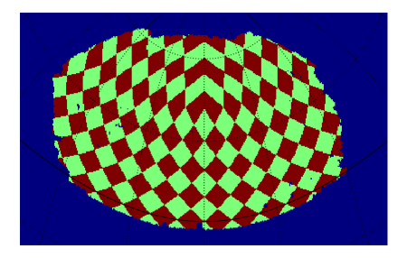
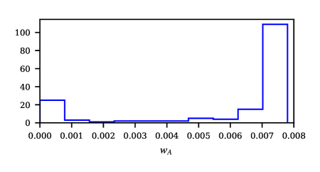
By construction the pixels have equal areas, so jackknife regions that are fully within the survey boundaries contain approximately the same number of galaxies. Pixels that intersect the survey boundary contain fewer galaxies, necessitating the weighting scheme introduced in (3.3). The distribution of weights for each region (which is closely related to the region area) is shown in Figure 7.
We are using a 350 bin correlation function and so it is clear that a jackknife covariance matrix for this correlation function, computed using 168 jackknife regions, must be singular, as anticipated above.
4.3 Fitting Results
As stated above, we use 900 of the QPM mocks to compute a sample covariance matrix. We then fit this, using the likelihood, against our model to make a single estimate of the shot-noise rescaling parameter . By leaving out individual mocks we can make a jackknife estimate of the uncertainty in , with our final result . This is the approach of O’Connell et al. (2016), and the result will be used as the fiducial value for .
| Approach | ||
|---|---|---|
| Sample fitting | 900 | |
| Jackknife fitting | 100 |
For each of the remaining 100 mocks we computed the jackknife covariance matrix using (3.9), then used the likelihood to fit the jackknife model and estimate . The result is 100 independent estimates of . A histogram of these 100 estimates is provided in Figure 8. Normal sample statistics on those estimates give . Note that 0.0009 is the error on the mean, and a jackknife fit using a single mock would give (on average) . The fitting results are summarised in 1. We find that the two fitting methods lead to compatible estimates of , validating the jackknife approach.
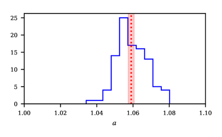
One surprising aspect of these fitting results is that the jackknife analysis of 100 mocks provides considerably more information about the shot-noise rescaling than does a sample analysis of 900 mocks. Intuitively, each jackknife region is large enough to provide information on its own about , and some of that information is lost when regions are combined in the sample analysis.
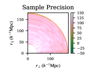
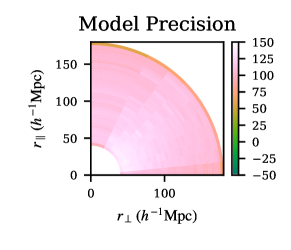
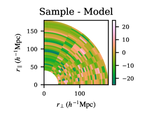
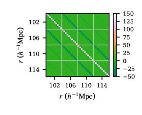
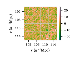
In Figure 9 we present the sample precision matrix , computed from 900 QPM mocks, and the model precision matrix , with as was found from the jackknife fits of the other 100 QPM mocks. The difference between the two matrices appears to be consistent with noise, providing additional evidence that the jackknife method has been successful.

4.4 Error Estimation for the Jackknife
We have demonstrated that the jackknife method can provide an accurate estimate of the shot-noise rescaling from a single survey volume. In situations where we have done this, it might be interesting to estimate the uncertainty in the estimate of . An additional jackknife can provide a reliable estimate of the uncertainty in , even with a single survey volume.
Recall that is the weight assigned to jackknife region when considering correlation function bin and that is the estimate of the correlation function in bin from region alone. We can estimate the covariance matrix with a single region excluded as follows. First, we recompute our weights and the average correlation function,
| (4.4) | ||||
| (4.5) |
then use the updated weights to compute the weighted jackknife covariance, with the single region omitted,
| (4.6) |
As in (3.9) the usual jackknife prescription in terms of dropped regions reduces to a rescaled sample covariance. We then fit the model against using the likelihood to find an estimate of the shot-noise rescaling, , with region left out.
Our next goal is to combine the into a jackknife estimate of obtained from the single survey volume. This first requires that we convert our bin-dependent weights, , into weights associated with the jackknife region alone, . A simple mean computed across the bins used in the analysis accomplishes this. We then perform a weighted jackknife to estimate :
| (4.7) | ||||
| (4.8) |
As the jackknife regions are not independent, we expect to provide a biased estimate of the true uncertainty . When we perform this analysis on 100 QPM mocks and average the results, we find
| (4.9) |
If we instead compute a sample variance on the values of computed from jackknife fits for those same 100 mocks we find , in surprisingly good agreement with the jackknife error estimate . This suggests that the jackknife error estimate provides a useful way to characterise the error on when it is estimated from a single survey volume.
4.5 Consequences for Measurement
So far we have focused on our ability to accurately and precisely estimate the shot-noise rescaling parameter . We now focus on the implications of that estimate for a hypothetical measurement of cosmological parameters. The primary complication is that measurements will involve a variety of modes – not just those associated with the cosmological parameters themselves, but also modes associated with additional nuisance parameters. Rather than choose a particular set of modes to examine, we focus on the average variance contributed by a single mode,
| (4.10) |
Under a uniform rescaling,
| (4.11) |
While the changes to the covariance matrix that we will consider are not uniform, we generally expect that when increases the parameter covariance matrix will increase as well, with changes in tied to changes in the parameter covariance matrix at the order-of-magnitude level.
We first consider whether the value of that we have determined, , is sufficiently different from to be of interest. If we look at the average variance, we find
| (4.12) | ||||
| (4.13) |
That is, if we ignore the shot-noise rescaling while performing a measurement, we expect the resulting parameter covariance matrix to be too small by roughly 9%. This establishes the necessity of applying the shot-noise rescaling.
The uncertainty in our estimate of will propagate through to uncertainty in the the covariance matrix. Using to measure this, we find that an uncertainty in of , as we would expect from a jackknife estimate using a single survey volume, corresponds to an uncertainty in of . In other words, for the BOSS-like survey considered here a 15% measurement of contributes roughly 1% to the error-on-the-error. At this point a variety of competing concerns about the error-on-the-error arise, including our approximation of contributions from the connected three- and four-point functions by additional shot noise, so we find the single-volume measurement of to be sufficiently accurate.
5 Outlook
Here we have generated a model covariance matrix for a BOSS-like survey. By construction, that model accurately reflects the long-distance physics and geometry of the survey. Short-distance physics is modelled by a single shot-noise rescaling parameter, and we have demonstrated that this parameter can be accurately and precisely calibrated using a single survey volume. The jackknife methods we have used for this calibration do not require significant computational resources beyond those required to pair-count the single survey volume. While we have validated this procedure using mock catalogues, we anticipate that future applications will use the actual survey as the single survey volume, obviating the need to use mock catalogues for covariance matrix estimation.
We emphasise that mock catalogues still play a vital role in estimating the size of systematic uncertainties. When generating mock catalogues there are clear trade-offs between accuracy and quantity. We hope that this method will allow limited computing resources to be focused on the former, by alleviating the need for the latter.
The larger lesson from our study is that because the shot-noise rescaling is determined by short-distance physics, it need not be estimated using covariance matrices that reflect the full survey geometry. While we anticipate that the jackknife approach will be very convenient, one can also imagine applications where several small-volume cubic mocks are used to estimate . We can even imagine applying the jackknife approach to those small volumes in order to increase the precision with which can be estimated.
While we have focused on a simple model for the short-distance physics of the survey, we do not expect our results to apply to this model alone. More accurate models of the short-distance physics might include several parameters governing redshift-space distortions and the connected 3- and 4-point functions. We expect the fitting methods described here could be readily applied to these models, with the caveat that parameters that are physically distinct could have degenerate, or nearly degenerate, impacts on the covariance matrix. The opportunity to fit such models either to the survey data themselves or to small-volume cubic mock catalogues could substantially reduce the computational requirements for next-generation surveys by removing the need to generate and analyse thousands of full-volume mock catalogues.
Acknowledgements
DJE is supported by U.S. Department of Energy grant DE-SC0013718 and as a Simons Foundation investigator.
References
- Bernstein (1994) Bernstein G. M., 1994, Astrophysical Journal, 424, 569
- Chuang et al. (2015) Chuang C.-H., et al., 2015, Mon. Not. Roy. Astron. Soc., 452, 686
- Dawson et al. (2013) Dawson K. S., et al., 2013, Astrophysical Journal, 145, 10
- Dodelson & Schneider (2013) Dodelson S., Schneider M. D., 2013, Phys.Rev., D88, 063537
- Doré et al. (2018) Doré O., et al., 2018, preprint (arXiv:1804.03628)
- Escoffier et al. (2016) Escoffier S., et al., 2016, preprint (arXiv:1606.00233)
- Górski et al. (2005) Górski K. M., Hivon E., Banday A. J., Wandelt B. D., Hansen F. K., Reinecke M., Bartelmann M., 2005, Astrophysical Journal, 622, 759
- Grieb et al. (2016) Grieb J. N., Sánchez A. G., Salazar-Albornoz S., Dalla Vecchia C., 2016, Mon. Not. Roy. Astron. Soc., 457, 1577
- Howlett & Percival (2017) Howlett C., Percival W. J., 2017, Mon. Not. Roy. Astron. Soc., 472, 4935
- Joachimi (2017) Joachimi B., 2017, Mon. Not. Roy. Astron. Soc., 466, L83
- Klypin & Prada (2018) Klypin A., Prada F., 2018, Monthly Notices of the Royal Astronomical Society, 478, 4602
- Laureijs et al. (2011) Laureijs R., et al., 2011, preprint, (arXiv:1110.3193)
- Levi et al. (2013) Levi M., et al., 2013, preprint (arXiv:1308.0847)
- Lippich et al. (2018) Lippich M., et al., 2018, preprint (arXiv:1806.09477)
- O’Connell et al. (2016) O’Connell R., Eisenstein D., Vargas M., Ho S., Padmanabhan N., 2016, Mon. Not. Roy. Astron. Soc., 462, 2681
- Padmanabhan et al. (2016) Padmanabhan N., White M., Zhou H. H., O’Connell R., 2016, Mon. Not. Roy. Astron. Soc., 460, 1567
- Pearson & Samushia (2016) Pearson D. W., Samushia L., 2016, Mon. Not. Roy. Astron. Soc., 457, 993
- Percival et al. (2014) Percival W. J., et al., 2014, Monthly Notices of the Royal Astronomical Society, 439, 2531
- Vargas-Magaña et al. (2018) Vargas-Magaña M., et al., 2018, Monthly Notices of the Royal Astronomical Society, 477, 1153
- White et al. (2014) White M., Tinker J. L., McBride C. K., 2014, Monthly Notices of the Royal Astronomical Society, 437, 2594
- Wishart (1928) Wishart J., 1928, Biometrika, 20A, 32
- Zhu et al. (2015) Zhu F., Padmanabhan N., White M., 2015, Monthly Notices of the Royal Astronomical Society, 451, 4755
- Zhu et al. (2018) Zhu F., et al., 2018, preprint (arXiv:1801.03038)
Appendix A Reducing Bias in Estimates of Precision Matrices
Although we often speak about different methods to estimate the covariance matrix, data analysis typically requires that we invert that covariance in order to estimate the precision matrix. Quite generally, noise on the estimate of the covariance matrix leads to bias in the estimate of the precision matrix. Suppose that provides an estimate of a covariance matrix , with some noise :
| (A.1) |
We depart slightly from the notation in the body of the paper and have in mind that the noisy estimate could be a sample covariance, jackknife estimate, or a noisy model. Our goal is to estimate , with the assumption that .
If we invert we find
| (A.2) |
The assumption that , eliminates the term, but the term at is nonzero in expectation:
| (A.3) |
When is a sample covariance matrix it follows the well-understood Wishart distribution (Wishart, 1928), and the series in (A.3) can be resummed to give
| (A.4) | ||||
| (A.5) |
It follows that provides an unbiased estimate of . When is not a sample covariance we do not expect it to follow the Wishart distribution, and require some other approach to manage the bias on . In the following we introduce a jackknife-inspired approach which can reduce (but not eliminate) this bias.
A.1 Quadratic Correction
We begin by assuming that rather than a single estimate of the covariance matrix, there are independent estimates:
| (A.6) |
In this paper the estimate is a result of numerical integration, so this is simply a matter of dividing the time dedicated to numerical integration among several independent runs, rather than using it for a single run. The most precise estimate of the model is then
As above, will be biased, but the multiple independent estimates will allow us to perform a separate estimate of this bias and subtract it off.
The inverse of is
| (A.7) | ||||
| (A.8) |
If the estimates are unbiased and independent, we have
| (A.9) | ||||
| (A.10) |
and so
| (A.11) |
We wish to estimate the quadratic bias. To do this we introduce
| (A.12) | ||||
| (A.13) |
Its inverse is
| (A.14) |
Our ultimate goal is to isolate the quadratic term. Toward that end it is beneficial to have a series that starts at , rather than , so we multiply by :
| (A.15) |
If we then average over , we find that the linear terms cancel:
| (A.16) |
In expectation, we have
| (A.17) |
and we recognise the same quadratic contribution as appeared in (A.11).
To actually perform the correction we introduce
| (A.18) |
The coefficients are chosen so that
| (A.19) |
so the quadratic contribution to the bias is eliminated. Note that the only assumptions we have made are that and that the estimates are independent from one another. Since the method does not rest on assumptions about the distribution of the noise, we expect it to be applicable to a wide variety of non-sample covariance matrices, not just the model described in this paper.
A.2 Application to our Model Precision Matrix
To illustrate this method of inversion we apply it to the model computed in section (2.2) of the main body of the paper. That approximates the covariance matrix for the 2-point galaxy correlation function in a BOSS-like survey, with the correlation function estimated in 350 bins of and . We generated independent estimates of the model covariance matrix.
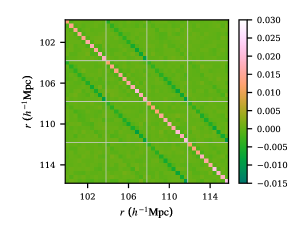
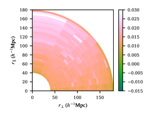
We begin by computing the introduced above. In figure 10 we show the result, with the primary corrections of . Although the we find is not proportional to the precision matrix, we find positive corrections on the diagonal, and smaller negative corrections for adjacent bins, reflecting the general structure of the precision matrix.
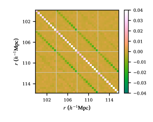
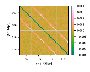
In order to verify that the correction introduced above actually yields a better inverse, we perform the following experiment. First, we split the independent estimates into five that will be used to estimate the covariance matrix, and five that will be used to generate an independent estimate of the precision matrix (by inverting the covariance matrix). We multiply these together to get a matrix close to the identity. To make the results more readable we present , which is the average of this residual matrix over all possible splits of the 10 estimates into two groups of five. Since our estimate of the covariance matrix is unbiased, systematic deviations of from the identity matrix result from bias in the precision matrix, introduced by inversion.
In figure 11 we plot a portion of without the quadratic correction above and then with the quadratic correction applied. Without the quadratic correction we find systematic deviations of from the identity at around 1%, as we would anticipate from the computed above. With the quadratic correction we find that the residuals are reduced by an order of magnitude, but not eliminated entirely. In other words the quadratic correction reduces the bias in the precision matrix, but does not provide an unbiased estimate.
A.3 Consistency of Fitting
We now perform an alternative check on the inverse of the model covariance matrix. In the main body of the paper we introduce a one-parameter family of model covariance matrices, , then fit the model against a sample covariance matrix, , computed using 900 QPM mocks. The shot-noise rescaling parameter can be estimated using two different likelihoods,
| (A.20) | ||||
| (A.21) |
If we have accurate estimates of and , the two approaches should lead to consistent estimates of . In this subsection we will show that this consistency is achieved if we apply the quadratic correction to .
We consider three different estimates of :
-
•
We will first estimate using the likelihood. Here we know that provides an unbiased estimate of , so this approach should yield an unbiased estimate of .
-
•
We then estimate using the likelihood, with the uncorrected inverse of .
-
•
Finally we estimate using the likelihood, with the quadratic correction applied to .
The fitting results are presented in table 2. In addition to the central values we make jackknife estimates (leaving out individual mocks) of the uncertainty in .
| Method | |
|---|---|
| likelihood | |
| likelihood, no correction | |
| likelihood, quadratic correction |
The fitting results in table 2 suggest a significant bias in when we use the uncorrected for fitting, but consistent results for when we apply the quadratic correction to . We note, however, that when testing to see if two sets of estimates for are consistent with one another it is not appropriate to simply add the uncertainties in each estimate in quadrature, as this ignores the possible issue of correlated errors in the and fittings. In order to address this we perform a second test on , the difference between as estimated using the likelihood and as estimated using the likelihood, with jackknife error bars computed for . The results, shown in table 3, clearly establish that in this application, the quadratic correction leads to consistent fitting results.
| Correction to | |
|---|---|
| None | |
| Quadratic |