Dynamical density response and optical conductivity in topological metals

Abstract

Topological metals continue to attract attention as novel gapless states of matter. While there by now exists an exhaustive classification of possible topologically nontrivial metallic states, their observable properties, that follow from the electronic structure topology, are less well understood. Here we present a study of the electromagnetic response of three-dimensional topological metals with Weyl or Dirac nodes in the spectrum, which systematizes and extends earlier pioneering studies. In particular, we argue that a smoking-gun feature of the chiral anomaly in topological metals is the existence of propagating chiral density modes even in the regime of weak magnetic fields. We also demonstrate that the optical conductivity of such metals exhibits an extra peak, which exists on top of the standard metallic Drude peak. The spectral weight of this peak is transferred from high frequencies and its width is proportional to the chiral charge relaxation rate.

I Introduction

Topological metal (TM) is a recently discovered new phase of matter. Armitage et al. (2018); Hasan et al. (2017); Yan and Felser (2017); Burkov (2018); Wan et al. (2011); Burkov and Balents (2011); Burkov et al. (2011); Xu et al. (2011); Young et al. (2012); Wang et al. (2012, 2013); Liu et al. (2014); Neupane et al. (2014); Xu et al. (2015); Lv et al. (2015a, b); Lu et al. (2015); Liu et al. (2017) It is characterized by topological invariants, defined on the Fermi surface, Volovik (2003); Haldane (2004); Volovik (2007); Murakami (2007) rather than in the whole Brillouin zone (BZ), as in topological insulators (TI). Such Fermi surface topological invariants arise as a consequence of monopole-like singularities in the electronic structure, Weyl nodes, whose significance was emphasized early on by Volovik and by Murakami. Volovik (2003); Murakami (2007)

Perhaps the most interesting feature of TM is that their electronic structure topology leads not only to spectroscopic manifestations in the form of edge states, Wan et al. (2011) a feature they share with TI, but also to nontrivial response. This novel response is usually described as being a consequence of the chiral anomaly, Zyuzin and Burkov (2012) which may be understood in the following way. While the appearance of gapless Weyl nodes in the spectrum has a topological origin, it also leads to an emergent symmetry, or an emergent conservation law, namely conservation of the chiral charge. This conservation law becomes increasingly more precise as the Fermi energy of the TM approaches the Weyl nodes. However, this apparent low-energy conservation law is violated when the system is coupled to an electromagnetic field. The origin of this violation lies in the fact that the chiral symmetry can never be an exact symmetry of a $(3+1)$-dimensional Dirac fermion on a lattice, as first pointed out by Nielsen and Ninomiya, Nielsen and Ninomiya (1983) as a single (or, more generally, an odd number) Dirac point in the BZ is topologically incompatible with the chiral symmetry. Thus, while the chiral symmetry appears to be present when one focuses only on states at the small Fermi surface, enclosing the Weyl points, the global lack of chiral symmetry manifests in the electromagnetic response of the system. This property is of great interest both because it has a topological origin and because it is contrary to one of the fundamental postulates of the standard theory of metals, which states that anything of observable consequence in a metal involves only states on the Fermi surface.

The chiral anomaly in TM has numerous predicted observable consequences, which include negative longitudinal magnetoresistance (LMR), Son and Spivak (2013); Burkov (2015) giant planar Hall effect (PHE), Burkov (2017); Nandy et al. (2017) and anomalous Hall effect. Burkov (2014) While most of these have already been observed experimentally in various TM materials, Xiong et al. (2015); Li et al. (2016, 2017); Kumar et al. (2017); Wang et al. (2018); Liu et al. (2017) none of these phenomena by themselves may be regarded as smoking-gun manifestations of the chiral anomaly, in the sense that all of them may in principle arise from unrelated sources, and these sources all have to be ruled out before the chiral anomaly origin may be claimed. An excellent discussion of these issues in the case of the negative LMR may be found in Ref. Liang et al., 2018.

As first discussed by Altland and Bagrets, Altland and Bagrets (2016) a truly unique feature of the chiral anomaly is the highly unusual dependence of the transport properties, such as the sample conductance, on the relevant length (and time or frequency, as will be shown in this paper) scales. In an ordinary three-dimensional (3D) metal the conductance scales linearly with the sample size $L$

$$G(L)=\sigma L,$$ (1)

where the Drude conductivity $\sigma$ is related to the density of states at the Fermi energy $g$ and the diffusion constant $D$ by the Einstein relation

$$\sigma=e^{2}gD.$$ (2)

Corrections to Eq. (1) are small in good metals, the small parameter being $1/k_{F}\ell$, where $k_{F}$ is the Fermi momentum ($\hbar=c=k_{B}=1$ units are used henceforth) and $\ell$ is the mean free path; the corrections arise only at very low temperatures as a result of quantum interference phenomena. The scaling of Eq. (1) is partly a consequence of the fact that, in an ordinary metal in the diffusive transport regime, i.e. at length scales, longer than the mean free path $\ell$ and time scales longer than the momentum relaxation time $\tau$, no intrinsic hydrodynamic (i.e. long) length scales remain, besides the sample size $L$.

However, as discussed in Ref. Altland and Bagrets, 2016, in a TM two additional hydrodynamic length scales emerge. These are the chiral charge diffusion length

$$L_{c}=\sqrt{D\tau_{c}},$$ (3)

where $\tau_{c}\gg\tau$ is the chirality relaxation time, and

$$L_{a}=D/\Gamma,$$ (4)

where $\Gamma=eB/2\pi^{2}g$ and $B$ is the applied magnetic field. $L_{a}$ is a new purely quantum mechanical magnetic-field-related length scale, which is distinct from the magnetic length $\ell_{B}=1/\sqrt{eB}$ and which arises from the chiral anomaly. It is related to the magnetic length as $L_{a}\sim\ell(k_{F}\ell_{B})^{2}$ and is thus much longer than the mean free path in the weak-field (quasiclassical) regime $k_{F}\ell_{B}\gg 1$, which we will be interested in here. Transport properties of TM may then be shown to depend strongly on the interplay of the three length scales: $L$, $L_{c}$, and $L_{a}$. Altland and Bagrets (2016); Burkov (2017) In particular, the strength of the negative LMR and the PHE depends on the parameter $L_{c}/L_{a}$, getting stronger as this ratio increases.

Particularly striking phenomena arise when $L_{a}<L<L_{c}^{2}/L_{a}$, Altland and Bagrets (2016) which is an extended and accessible range when $L_{c}/L_{a}\gg 1$. In this regime the sample conductance is given by

$$G(L)=\frac{e^{2}N_{\phi}}{2\pi},$$ (5)

where $N_{\phi}=L^{2}/2\pi\ell_{B}^{2}$ is the number of magnetic flux quanta, piercing the sample with cross-section area $L^{2}$. This means that in the regime $L_{a}<L<L_{c}^{2}/L_{a}$ the sample transports electric current as $N_{\phi}$ one-dimensional (1D) conduction channels and the conduction is ballistic and dissipationless [of course Eq. (5) only represents the dominant part of the conductance and ordinary dissipative Ohmic conduction is also present]. This is striking because it arises in a 3D metal with a Fermi surface and in the weak magnetic field regime $k_{F}\ell_{B}\gg 1$. The existence of such ballistic quasi-1D transport regime is a smoking-gun manifestation of the chiral anomaly in 3D TM.

In this paper we further elaborate on this striking property of TM and consider their related dynamical properties. In particular, we demonstrate that the quasi-1D transport regime manifests in dynamics as chiral propagating density modes, which exist in a range of wavevector values given by

$$L_{a}/L_{c}^{2}<q<1/L_{a}.$$ (6)

This “one-dimensionalization” of the electron dynamics is a unique property of TM, related to the chiral anomaly.

We also demonstrate that related phenomena exist in frequency-dependent properties of TM. In particular we demonstrate that the frequency dependence of the optical conductivity of TM has a non-Drude form, where an extra narrow peak exists at low frequencies, whose width scales as $1/\tau_{c}$ while height is a function of the ratio $L_{c}/L_{a}$. The spectral weight of this extra peak is transferred from high frequencies.

The rest of the paper is organized as follows. In Section II we calculate the full density response function of a simple model of a TM in an external magnetic field. We analyze the eigenmode structure of the density response function and demonstrate the presence of chiral propagating density modes when $L_{a}/L_{c}^{2}<q<1/L_{a}$. In Section III we relate the existence of these propagating chiral modes to observable transport properties of TM. We also demonstrate that similar phenomena exist in the frequency domain: we analyze the frequency dependence of the optical conductivity and point out its non-Drude nature. We conclude in Section IV with a brief discussion of the main results.

II Density response function of a topological metal

We start from the simplest model of a TM, which contains the necessary ingredients to capture the physics we want to describe. The simplest such model is the following model of a lattice Dirac fermion

$$H=t\gamma^{0}\gamma^{\mu}\sin k_{\mu}+\Delta({{\bf{k}}})\gamma^{0},$$ (7)

where

$$\Delta({{\bf{k}}})=t(3-\cos k_{x}-\cos k_{y}-\cos k_{z}),$$ (8)

and $\gamma^{\mu}$ are Dirac gamma matrices in, for example, the Weyl representation

$$\gamma^{0}=\tau^{x},\,\,\gamma^{i}=-i\tau^{y}\sigma^{i},\,\,i=1,2,3.$$ (9)

This model describes two Weyl nodes of opposite chirality at the $\Gamma$-point in the BZ (the effects we will be discussing do not depend on the momentum-space separation between the Weyl nodes). Since a single Dirac point in the BZ is incompatible with the chiral symmetry, Eq. (7) also has an essential property, shared by all real Weyl and Dirac semimetals, that the chiral symmetry (chiral charge conservation) is only an approximate low-energy symmetry of Eq. (7), which emerges when $H$ is expanded to linear order in ${{\bf{k}}}$ near the $\Gamma$-point. In this case we have

$$H=t\gamma^{0}\gamma_{\mu}k_{\mu},$$ (10)

and the chirality operator $\gamma^{5}=i\gamma^{0}\gamma^{1}\gamma^{2}\gamma^{3}=\tau^{z}$ commutes with $H$, which is no longer true once nonlinear terms are included. This gives a finite (but small) chiral charge relaxation rate, which is an essential property of a Weyl or Dirac semimetal.

We add a uniform magnetic field in the $z$-direction ${\bf{B}}=B\hat{z}$, and choose the Landau gauge for the vector potential ${\bf{A}}=xB\hat{y}$. We will ignore the Zeeman effect for simplicity. To find the eigenstates of $H$ in the presence of the magnetic field, we expand to first order in $k_{x,y}$, while keeping the full $k_{z}$ dependence. This is a good approximation in the regime of weak magnetic fields when $k_{F}\ell_{B}\gg 1$, which we will be interested in. For computational convenience we also make the following canonical transformation in the original Weyl representation of the gamma-matrices:

$$\tau^{x,y}\rightarrow\sigma^{z}\tau^{x,y},\,\,\sigma^{x,y}\rightarrow\tau^{z}\sigma^{x,y}.$$ (11)

This brings the Hamiltonian to the form

$$H=t(\sigma^{x}\pi_{x}+\sigma^{y}\pi_{y})+\hat{m}(k_{z})\sigma^{z},$$ (12)

where $\boldsymbol{\pi}=-i{\boldsymbol{\nabla}}+e{\bf{A}}$ is the canonical momentum and

$$\hat{m}(k_{z})=t\tau^{z}\sin k_{z}+\Delta(0,0,k_{z})\tau^{x}.$$ (13)

Diagonalizing Eq. (12), we find the eigenstate wavefunctions

$$|n,s,p,k_{y},k_{z}\rangle = z^{sp}_{n\uparrow\tau}(k_{z})|n-1,k_{y},k_{z},\uparrow,\tau\rangle$$ (14)

$$+ z^{sp}_{n\downarrow\tau}(k_{z})|n,k_{y},k_{z},\downarrow,\tau\rangle,$$

where $n$ is an integer Landau level index, $\uparrow,\downarrow$ label the two eigenvalues of $\sigma^{z}$, $\tau=\pm$ are the two eigenvalues of $\tau^{z}$, and $s,p=\pm$. Here and throughout sums over repeated indices will be implicit. The amplitudes $z^{sp}_{n\sigma\tau}(k_{z})$ may be regarded as components of an eigenvector $|z^{sp}_{n}(k_{z})\rangle=|v^{sp}_{n}(k_{z})\rangle\otimes|u^{p}(k_{z})\rangle$, where

$$|u^{p}_{n}(k_{z})\rangle=\frac{1}{\sqrt{2}}\left(\sqrt{1+p\frac{t\sin k_{z}}{m(k_{z})}},p\sqrt{1-p\frac{t\sin k_{z}}{m(k_{z})}}\right),$$

$$|v^{sp}_{n}(k_{z})\rangle=\frac{1}{\sqrt{2}}\left(\sqrt{1+sp\frac{m(k_{z})}{\epsilon_{n}(k_{z})}},s\sqrt{1-sp\frac{m(k_{z})}{\epsilon_{n}(k_{z})}}\right).$$

The corresponding energy eigenvalues are given by

$$\epsilon_{nsp}(k_{z})=s\epsilon_{n}(k_{z})=s\sqrt{2\omega_{B}^{2}n+m^{2}(k_{z})},$$ (16)

where $m(k_{z})=2t|\sin k_{z}|$, and $\omega_{B}=t/\ell_{B}$, for all $n\geq 1$. The lowest Landau level (LLL), corresponding to $n=0$, is special: it does not have the $s$ label and its eigenenergy and the corresponding eigenvector are given by

$$\epsilon_{0p}(k_{z})=-pm(k_{z}),$$ (17)

and

$$|v^{p}_{0}(k_{z})\rangle=(0,1).$$ (18)

We add to the Hamiltonian Eq. (12) random impurity potential $V({{\bf{r}}})$, which we take to be of the Gaussian white noise form with $\langle V({{\bf{r}}})\rangle=0$ and

$$\langle V({{\bf{r}}})V({{\bf{r}}}^{\prime})\rangle=\gamma^{2}\delta({{\bf{r}}}-{{\bf{r}}}^{\prime}).$$ (19)

We take the impurity potential to be independent of the spin and orbital pseudospin indices. Physically this means that the impurities are taken to be nonmagnetic and the potential is smooth enough that its spatial variation on the scale of the unit cell of the crystal is negligible. The last assumption is not essential, but does simplify the subsequent calculations.

We will evaluate the density response for the above model of a TM using the self-consistent Born approximation (SCBA) and the ladder approximation to perform the impurity averaging. This is a conserving approximation, meaning it preserves exact conservation laws and sum rules, and amounts physically to neglecting quantum interference effects. This is justified in the quasiclassical transport regime, which we will confine ourselves to: we assume that we are interested in the density response at length scales much longer than the inverse Fermi momentum and time scales much longer than the inverse Fermi energy; the impurity scattering is taken to be weak enough, so that $k_{F}\ell\gg 1$ and, as already mentioned, magnetic field is also assumed to be weak, which means $k_{F}\ell_{B}\gg 1$. Finally, we will assume that the Fermi energy is close to the Dirac point $\epsilon_{F}\ll t$ (but $\epsilon_{F}\tau\gg 1$), which defines the regime of a TM. The last condition ensures the near conservation of the chiral charge, as will be seen explicitly below.

The calculation of the SCBA impurity self-energy in a similar model has already been discussed in detail in Ref. Burkov, 2015. We will thus omit the details of this calculation here and simply quote the result. One obtains that in the quasiclassical transport regime the impurity scattering rate is independent of both the Landau level index $n$ and the longitudinal momentum component $k_{z}$ and is given by the standard SCBA expression

$$\frac{1}{\tau}=\frac{\pi\gamma^{2}g}{2},$$ (20)

where the density of states at the Fermi energy is given by

$$g=\frac{\epsilon_{F}}{\pi t^{2}}\int_{-\pi}^{\pi}\frac{dk_{z}}{2\pi}\Theta[\epsilon_{F}-m(k_{z})],$$ (21)

$\Theta(x)$ being the Heaviside step function.

We evaluate the density response function by summing the impurity ladder diagrams. We start from the most general retarded density matrix response function, defined as

$$\chi_{\alpha_{1}\alpha_{2},\alpha_{3}\alpha_{4}}({{\bf{r}}},t|{{\bf{r}}}^{\prime},t^{\prime})$$ (22)

$$= -i\Theta(t-t^{\prime})\langle[\varrho^{\vphantom{{\dagger}}}_{\alpha_{1}\alpha_{2}}({{\bf{r}}},t),\varrho^{{\dagger}}_{\alpha_{3}\alpha_{4}}({{\bf{r}}}^{\prime},t^{\prime})]\rangle,$$

where the density matrix is defined as

$$\varrho_{\alpha_{1}\alpha_{2}}({{\bf{r}}},t)=\Psi^{{\dagger}}_{\alpha_{2}}({{\bf{r}}},t)\Psi^{\vphantom{{\dagger}}}_{\alpha_{1}}({{\bf{r}}},t),$$ (23)

and $\alpha=(\sigma\tau)$ is a composite index, which encodes both the spin and orbital pseudospin labels.

The standard procedure to find the real-time response function Eq. (22) is to start from the corresponding imaginary-time response function

$$\chi_{\alpha_{1}\alpha_{2},\alpha_{3}\alpha_{4}}({{\bf{r}}},\tau|{{\bf{r}}}^{\prime},\tau^{\prime})$$ (24)

$$= -{\cal G}_{\alpha_{1}\alpha_{3}}({{\bf{r}}},{{\bf{r}}}^{\prime},\tau-\tau^{\prime}){\cal G}_{\alpha_{4}\alpha_{2}}({{\bf{r}}}^{\prime},{{\bf{r}}},\tau^{\prime}-\tau),$$

where ${\cal G}_{\alpha\alpha^{\prime}}({{\bf{r}}},{{\bf{r}}}^{\prime},\tau-\tau^{\prime})$ is the exact imaginary-time Green’s function, which depends on both ${{\bf{r}}}$ and ${{\bf{r}}}^{\prime}$ separately due to both the lack of translational symmetry in the presence of a random impurity potential, and the lack of gauge invariance in the presence of an external magnetic field. One then performs impurity averaging, which restores translational invariance in the density response function and gives

$$\chi_{\alpha_{1}\alpha_{2},\alpha_{3}\alpha_{4}}({\bf{q}},i\Omega)=\frac{1}{\beta}\sum_{i\omega}{\cal P}_{\alpha_{1}\alpha_{2},\alpha_{3}\alpha_{4}}({\bf{q}},i\omega,i\omega+i\Omega),$$ (25)

where

$${\cal P}_{\alpha_{1}\alpha_{2},\alpha_{3}\alpha_{4}}({{\bf{r}}}-{{\bf{r}}}^{\prime},i\omega,i\omega+i\Omega)$$ (26)

$$= -\langle{\cal G}_{\alpha_{1}\alpha_{3}}({{\bf{r}}},{{\bf{r}}}^{\prime},i\omega+i\Omega){\cal G}_{\alpha_{4}\alpha_{2}}({{\bf{r}}}^{\prime},{{\bf{r}}},i\omega)\rangle,$$

is the impurity-averaged generalized polarization bubble, and $\beta=1/T$ is the inverse temperature. In the quasiclassical regime we are interested in, ${\cal P}$ may be evaluated by summing all the SCBA diagrams for the impurity self-energy and the ladder vertex corrections, as shown in Fig. 1. The result of this diagram summation may be written in a shorthand matrix notation as

$${\cal P}={\cal P}^{0}{\cal D},$$ (27)

where ${\cal P}^{0}$ is the bare polarization bubble, in which only the self-energy corrections are included

$${\cal P}^{0}_{\alpha_{1}\alpha_{2},\alpha_{3}\alpha_{4}}({{\bf{r}}}-{{\bf{r}}}^{\prime},i\omega,i\omega+i\Omega)$$ (28)

$$= -{\cal G}_{\alpha_{1}\alpha_{3}}({{\bf{r}}},{{\bf{r}}}^{\prime},i\omega+i\Omega){\cal G}_{\alpha_{4}\alpha_{2}}({{\bf{r}}}^{\prime},{{\bf{r}}},i\omega).$$

${\cal G}_{\alpha\alpha^{\prime}}({{\bf{r}}},{{\bf{r}}}^{\prime},i\omega)$ here is the disorder-averaged SCBA Green’s function, which still depends on ${{\bf{r}}}$ and ${{\bf{r}}}^{\prime}$ separately since it is a gauge-dependent quantity in the presence of an external magnetic field. The vertex part ${\cal D}$, which is also known as the diffusion propagator, or diffuson, satisfies the following Bethe-Salpeter equation

$${\cal D}=1+{\cal I}{\cal D},$$ (29)

where ${\cal I}\equiv\gamma^{2}{\cal P}^{0}$. The solution of this equation is

$${\cal D}=(1-{\cal I})^{-1}.$$ (30)

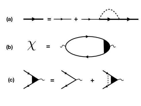
Figure 1: Diagrammatic representation of (a) SCBA Green’s function. Thin line represents the bare Green’s function, thick line is the SCBA impurity-averaged Green’s function and the dashed line represents the disorder potential correlator $\langle V({{\bf{r}}})V({{\bf{r}}}^{\prime})\rangle=\gamma^{2}\delta({{\bf{r}}}-{{\bf{r}}}^{\prime})$. (b) Density response function $\chi$. (c) Bethe-Salpeter equation for the diffusion vertex ${\cal D}$.

To obtain the real-time retarded response function we analytically continue to real frequency $i\Omega\rightarrow\Omega+i\eta$, which gives

$$\chi({\bf{q}},\Omega)=\int_{-\infty}^{\infty}\frac{d\epsilon}{2\pi i}n_{F}(\epsilon)\left[{\cal P}({\bf{q}},\epsilon+i\eta,\epsilon+\Omega+i\eta)\right.$$ (31)

$$- \left.{\cal P}({\bf{q}},\epsilon-i\eta,\epsilon+\Omega+i\eta)+{\cal P}({\bf{q}},\epsilon-\Omega-i\eta,\epsilon+i\eta)\right.$$

$$- \left.{\cal P}({\bf{q}},\epsilon-\Omega-i\eta,\epsilon-i\eta)\right].$$

In the low-frequency limit, when $\Omega\ll\epsilon_{F}$, this simplifies to

$$\chi({\bf{q}},\Omega) = -\frac{i\Omega}{2\pi}{\cal P}({\bf{q}},-i\eta,\Omega+i\eta)$$ (32)

$$- \frac{1}{\pi}\int_{-\infty}^{\infty}d\epsilon\,n_{F}(\epsilon)\textrm{Im}{\cal P}({\bf{q}},\epsilon+i\eta,\epsilon+\Omega+i\eta)$$

$$\equiv \chi^{I}({\bf{q}},\Omega)+\chi^{II}({\bf{q}},\Omega).$$

The physical meaning of the two contributions to the density response function, $\chi^{I}$ and $\chi^{II}$, is that $\chi^{I}$ arises from states on the Fermi surface, while all filled states contribute to $\chi^{II}$. $\chi^{II}$ thus represents equilibrium part of the response and is easily shown to be a diagonal matrix, with the nonzero matrix elements equal to $-g$. On the other hand, $\chi^{I}$ represents the dynamical nonequilibrium part of the density response and is given by

$$\chi^{I}({\bf{q}},\Omega)=-\frac{i\Omega}{2\pi\gamma^{2}}{\cal I}({\bf{q}},\Omega){\cal D}({\bf{q}},\Omega),$$ (33)

where

$${\cal I}_{\alpha_{1}\alpha_{2},\alpha_{3}\alpha_{4}}({\bf{q}},\Omega)=\frac{\gamma^{2}}{L^{3}}\int d^{3}r\,d^{3}r^{\prime}e^{-i{\bf{q}}\cdot({{\bf{r}}}-{{\bf{r}}}^{\prime})}$$ (34)

$$\times G^{R}_{\alpha_{1}\alpha_{3}}({{\bf{r}}},{{\bf{r}}}^{\prime},\Omega)G^{A}_{\alpha_{4}\alpha_{2}}({{\bf{r}}}^{\prime},{{\bf{r}}},0),$$

$G^{R,A}$ being the retarded and advanced real-time impurity-averaged SCBA Green’s functions. They are explicitly given by

$$G^{R,A}_{\alpha\alpha^{\prime}}({{\bf{r}}},{{\bf{r}}}^{\prime},\omega)$$

$$= \sum_{nspk_{y}k_{z}}\frac{\langle{{\bf{r}}},\alpha|n,s,p,k_{y},k_{z}\rangle\langle n,s,p,k_{y},k_{z}|{{\bf{r}}}^{\prime},\alpha^{\prime}\rangle}{\omega-\xi_{nsp}(k_{z})\pm i/2\tau},$$

where $\xi_{nsp}(k_{z})\equiv\epsilon_{nsp}(k_{z})-\epsilon_{F}$.

For a general direction of the wavevector ${\bf{q}}$, the evaluation of ${\cal I}({\bf{q}},\Omega)$ is severely complicated by the fact that contributions of different Landau levels are mixed in Eq. (34). This is not the case only when ${\bf{q}}=q\hat{z}$, when translational symmetry in the $xy$-plane leads to decoupling of the individual Landau level contributions. Fortunately, this is in fact the case of primary interest to us, since the chiral anomaly leads to unusual transport phenomena in the direction of the magnetic field. Thus we will take ${\bf{q}}=q\hat{z}$ henceforth.

In this case the evaluation of ${\cal I}({\bf{q}},\Omega)$ is relatively straightforward, particularly in the weak magnetic field regime $k_{F}\ell_{B}\gg 1$ that we are interested in. An additional simplification arises from the fact that we are not interested in the whole $16\times 16$ matrix ${\cal I}$, which contains a lot of unnecessary information. We are interested only in the response of conserved, or nearly conserved, quantities, which will always dominate everything else at long times and long distances. In a generic TM, we expect only two such quantities to exist: the electric charge, which is strictly conserved, and the chiral charge, whose near conservation is a defining property of a TM, as discussed above. Thus we may project the original $16\times 16$ matrix onto the $2\times 2$ subspace, describing the coupled transport of the electric and the chiral charge, which is accomplished as

$${\cal I}_{ab}({\bf{q}},\Omega)=\frac{1}{4}\Gamma^{a}_{\alpha_{2}\alpha_{1}}{\cal I}_{\alpha_{1}\alpha_{2},\alpha_{3}\alpha_{4}}({\bf{q}},\Omega)\Gamma^{b}_{\alpha_{3}\alpha_{4}},$$ (36)

where $a,b=0,5$, corresponding to the electric $(0)$ or chiral $(5)$ charges, and $\Gamma^{a,b}$ are the corresponding operators, i.e.

$$\Gamma^{0}=\tau^{0}\sigma^{0}=1,\,\,\Gamma^{5}=\tau^{z}\sigma^{0}=\tau^{z}.$$ (37)

After a tedious, but straightforward, calculation, we obtain

$${\cal I}_{00}(q,\Omega) = \frac{i}{2q\ell}\ln\left(\frac{1-i\Omega\tau-iq\ell}{1-i\Omega\tau+iq\ell}\right),$$

$${\cal I}_{55}(q,\Omega) = \left[\frac{i}{2q\ell}-\frac{i(\epsilon_{F}/t)^{2}(1-i\Omega\tau)^{4}}{8(q\ell)^{5}}\right]\ln\left(\frac{1-i\Omega\tau-iq\ell}{1-i\Omega\tau+iq\ell}\right)-\frac{(\epsilon_{F}/t)^{2}(1-i\Omega\tau)}{12(q\ell)^{2}}+\frac{(\epsilon_{F}/t)^{2}(1-i\Omega\tau)^{3}}{4(q\ell)^{4}},$$

$${\cal I}_{05}(q,\Omega) = {\cal I}_{50}(q,\Omega)=\frac{i}{2(k_{F}\ell_{B})^{2}}\frac{q\ell}{(1-i\Omega\tau)^{2}+(q\ell)^{2}}.$$ (38)

Substituting this into Eq. (33), we obtain the dynamical nonequilibrium contribution to the density response $\chi^{I}(q,\Omega)$, while the equilibrium contribution is a diagonal matrix given by

$$\chi^{II}_{00}(q,\Omega)=\chi^{II}_{55}(q,\Omega)=-g,$$ (39)

as already mentioned above.

A comment is in order here. As can be seen from Eq. (II), only the off-diagonal matrix element ${\cal I}_{05}$ depends on the magnetic field. This is true in the quasiclassical limit $k_{F}\ell_{B}\gg 1$ only, and is a consequence of the fact that in this limit we may ignore the effect of the magnetic field on the density of states. Summation over the Landau level index $n$, which arises when evaluating Eq. (II), may in this case be replaced by integration and the magnetic field dependence disappears to leading order in $1/k_{F}\ell_{B}$. In contrast, the off-diagonal matrix element ${\cal I}_{05}$ arises entirely from the contribution of the $n=0$ Landau level. This contribution is proportional to $1/(k_{F}\ell_{B})^{2}$, but leads to large effects at long length scales and long times, as will be seen below, provided $\tau_{c}/\tau\gg 1$.

Eqs. (32), (33), (II) and (39) give a general expression for the density response function of a TM in the quasiclassical regime

$$\chi(q,\Omega)=-g[i\Omega\tau{\cal I}(q,\Omega){\cal D}(q,\Omega)+1].$$ (40)

This expression is valid in either diffusive $\Omega\tau,q\ell\ll 1$ or ballistic $\Omega\tau,q\ell\gg 1$ limits and may be used, in particular, to study the ballistic-diffusive crossover regime. We will start by analyzing the two limits.

II.1 Ballistic regime

In this regime all components of the matrix ${\cal I}$ are small and thus ${\cal D}\approx 1$. Physically this means that we are looking at short length and time scales at which the impurity scattering may be ignored. While the response function $\chi(q,\Omega)$ is a $2\times 2$ matrix, only its $\chi_{00}(q,\Omega)$ component describes observable density response. Taking the limit $\Omega\tau,q\ell\rightarrow\infty$ in Eqs. (II), (40) we obtain

$$\chi_{00}(q,\Omega)=-g\left[1+\frac{\Omega}{2qt}\ln\left(\frac{\Omega-qt+i\eta}{\Omega+qt+i\eta}\right)\right].$$ (41)

This is just the familiar Lindhard function (in the limit $q\ll k_{F}$ and $\Omega\ll\epsilon_{F}$), describing the density response of a clean Fermi liquid with the Fermi velocity $t$. The imaginary part of $\chi_{00}(q,\Omega)$, which is determined by the branch cuts of the Lindhard function

$$\textrm{Im}\chi_{00}(q,\Omega)=g\frac{\pi\Omega}{2qt}\,\Theta(qt-|\Omega|),$$ (42)

describes the excitation spectrum of the Fermi liquid, which forms a particle-hole continuum. Thus in the ballistic regime and in the weak magnetic field limit chiral anomaly has no effect on the density response of a TM [its effects appear only at order $1/(k_{F}\ell_{B})^{2}$, which is negligible compared to Eq. (41)]. This of course will no longer be true if we tune the Fermi energy to zero (i.e. to the ideal Weyl or Dirac semimetal limit), but this is a fine-tuned, non-generic situation, and is of somewhat less interest for this reason.

II.2 Diffusive regime

The situation is much more interesting in the diffusive limit $\Omega\tau,q\ell\ll 1$. In this case ${\cal I}\approx 1$, and multiple impurity scattering needs to be taken into account. Expanding in Taylor series in $\Omega\tau$ and $q\ell$, we obtain

$${\cal I}_{00}(q,\Omega) \approx 1+i\Omega\tau-Dq^{2}\tau,$$

$${\cal I}_{05}(q,\Omega) = {\cal I}_{50}(q,\Omega)\approx i\Gamma q\tau,$$

$${\cal I}_{55}(q,\Omega) \approx 1+i\Omega\tau-\tau/\tau_{c}-Dq^{2}\tau.$$ (43)

Here $D=t^{2}\tau/3=t\ell/3$ is the diffusion constant,

$$\Gamma=\frac{eB}{2\pi^{2}g}=\frac{t}{2(k_{F}\ell_{B})^{2}},$$ (44)

is a new transport coefficient, which describes the chiral-anomaly-induced coupling between the electric and the chiral charge densities, and

$$\frac{1}{\tau_{c}}=\frac{\epsilon_{F}^{2}}{20\,t^{2}\tau},$$ (45)

is the chiral charge relaxation rate. Note that the fact the chiral charge relaxation rate vanishes in the limit $\epsilon_{F}\rightarrow 0$ is a consequence of our assumption that the impurity potential is diagonal in the spin and orbital indices and thus commutes with the chiral charge operator $\gamma^{5}=\tau^{z}$. In general this is not the case and we can expect some residual chiral charge relaxation even in the $\epsilon_{F}\rightarrow 0$ limit.

In the diffusive regime the dynamics of the density response is determined by the poles of the diffusion propagator ${\cal D}$, instead of the branch cuts of the response function, as in the ballistic limit. From Eq. (II.2), the inverse diffusion propagator is given by

$${\cal D}^{-1}(q,\Omega)=\left(\begin{array}[]{cc}-i\Omega\tau+Dq^{2}\tau&-i\Gamma q\tau\\ -i\Gamma q\tau&-i\Omega\tau+\tau/\tau_{c}+Dq^{2}\tau\end{array}\right),$$ (48)

The zeros of the determinant of this matrix determine the eigenmode frequencies

$$\Omega_{\pm}=\pm\Omega_{0}-i(Dq^{2}+1/2\tau_{c}),$$ (50)

where

$$\Omega_{0}=\sqrt{\Gamma^{2}q^{2}-1/4\tau_{c}^{2}}.$$ (51)

The diffusion propagator itself may then be written as

$${\cal D}(q,\Omega) = \frac{1/\tau}{(\Omega-\Omega_{+})(\Omega-\Omega_{-})}$$ (54)

$$\times \left(\begin{array}[]{cc}i\Omega-Dq^{2}-1/\tau_{c}&-i\Gamma q\\ -i\Gamma q&i\Omega-Dq^{2}\end{array}\right).$$

Taking into account that in the diffusive regime ${\cal I}\approx 1$, we obtain from Eq. (40)

$$\chi(q,\Omega)\approx-g[i\Omega\tau{\cal D}(q,\Omega)+1],$$ (55)

which gives the following explicit expression for the $00$ component of the matrix response function, which corresponds to the observable electric charge density response

$$\chi_{00}(q,\Omega)=g\left[\frac{\Omega(\Omega+i/\tau_{c}+iDq^{2})}{(\Omega-\Omega_{+})(\Omega-\Omega_{-})}-1\right].$$ (56)

We now note that the frequency $\Omega_{0}$ is purely imaginary at the smallest momenta when

$$q<\frac{1}{2\Gamma\tau_{c}}=\frac{L_{a}}{2L_{c}^{2}}\equiv\frac{1}{L_{*}},$$ (57)

where we have introduced two new length scales

$$L_{c}=\sqrt{D\tau_{c}},$$ (58)

which has the meaning of the chiral charge diffusion length and

$$L_{a}=\frac{D}{\Gamma}=\frac{2}{3}\ell(k_{F}\ell_{B})^{2}.$$ (59)

$L_{a}$ is a magnetic-field-related length scale, distinct from the magnetic length, which arises from the chiral anomaly. It is a long hydrodynamic length scale in the weak magnetic field regime, in the sense that $L_{a}\gg\ell$, but it may still be much smaller that either the chiral charge diffusion length $L_{c}$ or the sample size $L$. In fact, the ratio $L_{c}/L_{a}$ quantifies the strength of the chiral-anomaly-related density response phenomena, as will be seen below.

Thus when $q<1/L_{*}$ the eigenfrequencies of the diffusion propagator are purely imaginary, which corresponds to ordinary diffusion (nonpropagating) modes. However, when $q>1/L_{*}$ (which may be a very small momentum when the ratio $L_{c}/L_{a}$ is large), $\Omega_{0}$ is real, which signals the emergence of a pair of propagating modes in this regime. The modes are only weakly damped as long as

$$\Omega_{0}\approx\Gamma q>Dq^{2},$$ (60)

which defines the upper limit on the wavevector $q=1/L_{a}$, above which the propagating modes disappear. The propagating modes thus exist in the interval

$$1/L_{*}<q<1/L_{a}.$$ (61)

This interval is significant when $L_{c}/L_{a}\gg 1$.

Within this interval of $q$ the density response function takes the following approximate form

$$\chi_{00}(q,\Omega)=g\frac{\Omega_{0}^{2}}{(\Omega+iDq^{2})^{2}-\Omega_{0}^{2}},$$ (62)

where $\Omega_{0}=\Gamma q$. This is the density response function of an effective 1D system with the Fermi velocity $\Gamma=t/2(k_{F}\ell_{B})^{2}\ll t$. Note that this is very different from the 1D response one would obtain in a TM in the quantum limit $k_{F}\ell_{B}<1$, when only the lowest $n=0$ Landau level contributes to the density response. In this case one gets $N_{\phi}$ 1D modes, which correspond to $N_{\phi}$ orbital states within the LLL. The Fermi velocity of these 1D modes is equal to the microscopic Fermi velocity $t$. In our case, while the ultimate origin of the 1D dynamics is still the LLL, its emergence is only possible in the diffusive regime and thus requires multiple impurity scattering. The corresponding Fermi velocity $\Gamma$ is proportional to the applied magnetic field and is much smaller than $t$ in the quasiclassical weak-field regime. Such effectively 1D density response, with propagating rather than diffusive density dynamics, which exists in a 3D metal with a large Fermi surface ($k_{F}\ell\gg 1$) in a weak magnetic field ($k_{F}\ell_{B}\gg 1$) is a truly unique feature of TM and should be regarded as their true smoking-gun characteristic.

On the other hand, when $L_{a}>L_{c}$, propagating modes do not exist for any $q$ and one obtains a pair of standard diffusion modes

$$\Omega_{+}=-iDq^{2},\,\,\Omega_{-}=-iDq^{2}-i/\tau_{c},$$ (63)

which correspond to independent diffusion of the electric and the chiral charge densities.

III Transport in topological metals

It is very useful to also look at the transport properties, which follow from the density response, described in Section II. In addition to providing further insight into the physical meaning of the results, discussed in the previous section, this will also allow us to calculate experimentally measurable physical quantities, such as the frequency- and scale-dependent conductivity.

III.1 Scale-dependent conductance

It is easy to show that Eqs. (54) and (55) for the diffusion propagator and the generalized density response function are equivalent to the following transport equation in real space and time, that the electric $n_{0}$ and chiral $n_{5}$ charge densities must satisfy

$$\frac{\partial n_{0}}{\partial t} = D{\boldsymbol{\nabla}}^{2}(n_{0}+gV_{0})+{\boldsymbol{\Gamma}}\cdot{\boldsymbol{\nabla}}(n_{5}+gV_{5}),$$

$$\frac{\partial n_{5}}{\partial t} = D{\boldsymbol{\nabla}}^{2}(n_{5}+gV_{5})-\frac{n_{5}+gV_{5}}{\tau_{c}}+{\boldsymbol{\Gamma}}\cdot{\boldsymbol{\nabla}}(n_{0}+gV_{0}),$$

where $V_{0}$ and $V_{5}$ are external electric and chiral potentials correspondingly and we have generalized to an arbitrary magnetic field direction, which is why the coefficient ${\boldsymbol{\Gamma}}\propto{\bf{B}}$ has become a vector. The chiral potential $V_{5}$ may arise, for example, in a situation when the inversion symmetry is broken, in which case the Weyl nodes of different chirality will generally be located at different energies, $V_{5}$ being precisely this energy difference. Otherwise this should simply be regarded as a fictitious potential, which couples linearly to the chiral charge $n_{c}$. Indeed, Fourier transforming Eq. (III.1) we obtain

$${\cal D}^{-1}(q,\Omega)\left(\begin{array}[]{c}n_{0}\\ n_{5}\end{array}\right)=-g\left[i\Omega\tau+{\cal D}^{-1}(q,\Omega)\right]\left(\begin{array}[]{c}V_{0}\\ V_{5}\end{array}\right).$$ (69)

This gives

$$\left(\begin{array}[]{c}n_{0}\\ n_{5}\end{array}\right)=-g[i\Omega\tau{\cal D}(q,\Omega)+1]\left(\begin{array}[]{c}V_{0}\\ V_{5}\end{array}\right),$$ (75)

which is equivalent to Eq. (55).

Solving Eq. (III.1) in the steady state, assuming a uniform sample of linear size $L$, attached to normal metal leads (in which the chiral electrochemical potential $n_{5}+gV_{5}=0$) in the $z$-direction (i.e. the current flows along the magnetic field), one obtains the following expression for the scale-dependent sample conductance Altland and Bagrets (2016); Burkov (2017)

$$G(L)=\frac{e^{2}N_{\phi}}{2\pi}F(L/L_{a},L/L_{c}),$$ (76)

where the scaling function $F(x,y)$ is given by

$$F(x,y)=\frac{(1+y^{2}/x^{2})^{3/2}}{\frac{y^{2}}{2x}\sqrt{1+y^{2}/x^{2}}+\tanh\left(\frac{x}{2}\sqrt{1+y^{2}/x^{2}}\right)}.$$ (77)

This scaling function exhibits crossover behaviors which exactly match the corresponding crossovers in the wavevector dependence of the diffusion modes, described in Section II.

Indeed, when $x\ll y$, which means $L_{a}\gg L_{c}$, we have $F(x,y)\approx 2/x$, which gives

$$G(L)\approx e^{2}gDL=\sigma L,$$ (78)

which is simply the standard Ohmic conductance, with a small magnetic-field dependent correction, which goes as $(L_{c}/L_{a})^{2}$, and which we have ignored here for the sake of brevity. Burkov (2017) This corresponds to the regime, in which we have two independent diffusion modes, given by Eq. (63), corresponding to independent diffusion of the electric and the chiral charges.

On the other hand, when $L_{a}\ll L_{c}$, or $x\gg y$, we obtain

$$F(x,y)\approx\frac{1}{y^{2}/2x+\tanh(x/2)}.$$ (79)

This exhibits a regime of quasiballistic conductance with

$$G(L)\approx\frac{e^{2}N_{\phi}}{2\pi},$$ (80)

which is realized when

$$L_{a}<L<L_{*}.$$ (81)

This corresponds precisely to the range of the wavevectors $q$ in Eq. (61), for which propagating modes exist when $L_{a}\ll L_{c}$. Thus, one of the observable manifestations of the existence of quasi-1D propagating modes in a TM is the quasiballistic conductance, given by Eq. (80).

It is instructive to see what the quasiballistic conductance regime corresponds to directly in terms of the transport equations Eq. (III.1). In this regime both the second derivative $D{\boldsymbol{\nabla}}^{2}n_{0,5}$ and the relaxation $n_{5}/\tau_{c}$ terms may be ignored and we obtain

$$\frac{\partial n_{0}}{\partial t} = \Gamma\frac{\partial n_{5}}{\partial z},$$

$$\frac{\partial n_{5}}{\partial t} = \Gamma\frac{\partial n_{0}}{\partial z}.$$ (82)

Introducing the left- and right-handed charges as $n_{R,L}=(n_{0}\pm n_{5})/2$ we obtain

$$\frac{\partial n_{R}}{\partial t} = \Gamma\frac{\partial n_{R}}{\partial z},$$

$$\frac{\partial n_{L}}{\partial t} = -\Gamma\frac{\partial n_{L}}{\partial z}.$$ (83)

Eq. (III.1) describes two chiral bosonic density modes, which propagate along and opposite to the direction of the applied magnetic field. Such “bosonization” of the electron dynamics, which occurs in a 3D metal in a weak quasiclassical magnetic field, is a characteristic smoking-gun feature of a TM.

Eq. (III.1) means, in particular, that a density disturbance, created in a TM in magnetic field, with split into two chiral modes, which will propagate ballistically in opposite directions, spatially separating electrons of different chirality. It might be possible to detect this effect optically. Ma et al. (2017)

III.2 Optical conductivity

Optical conductivity of TM has been studied before, with a focus mostly on the interband transition effects. Tabert and Carbotte (2016); Ahn et al. (2017); Roy et al. (2016); Sun and Wang (2017); Neubauer et al. (2018) Here we will demonstrate that low-frequency intraband optical conductivity is qualitatively affected by the chiral anomaly, which has not been noticed before.

From the general expression for the density response function Eq. (40) we may easily obtain the frequency-dependent conductivity. Indeed, electric charge conservation requires that

$$\sigma_{zz}(\Omega)=-e^{2}\lim_{q\rightarrow 0}\frac{i\Omega}{q^{2}}\chi_{00}(q,\Omega).$$ (84)

A straightforward calculation then gives

$$\sigma_{zz}(\Omega)=\frac{\sigma}{1-i\Omega\tau}\frac{1-i\Omega\tau_{c}+(L_{c}/L_{a})^{2}}{1-i\Omega\tau_{c}},$$ (85)

where $\sigma=e^{2}gD$ is the zero-field DC conductivity. Evaluating the real part, one obtains

$$\textrm{Re}\,\sigma_{zz}(\Omega)=\frac{\sigma}{1+\Omega^{2}\tau^{2}}\left[1+\left(\frac{L_{c}}{L_{a}}\right)^{2}\frac{1-\Omega^{2}\tau\tau_{c}}{1+\Omega^{2}\tau_{c}^{2}}\right].$$ (86)

Eq. (86) is one of the main new results of this paper. The prefactor in Eq. (86) is the standard Drude expression for the optical conductivity of a metal. The part in the square brackets is a correction that arises in a TM as a consequence of the chiral anomaly. This correction represents transfer of the spectral weight from high frequencies into a new low-frequency peak, whose width scales with the chiral charge relaxation rate $1/\tau_{c}$, while height is proportional to the ratio $(L_{c}/L_{a})^{2}$. Importantly, Eq. (86) satisfies the exact $f$-sum rule

$$\int_{0}^{\infty}d\Omega\,\,\textrm{Re}\,\sigma_{zz}(\Omega)=\frac{\pi\sigma}{2\tau},$$ (87)

which means that the appearance of the new low-frequency peak indeed represents spectral weight transfer, as it should, see Fig. 2.

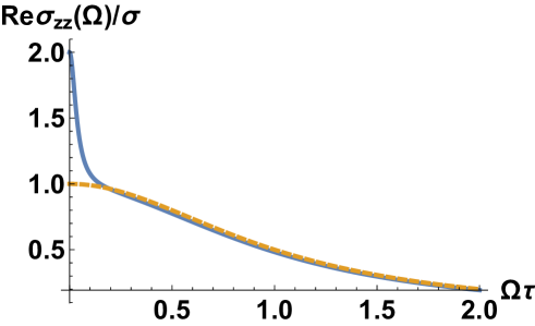
Figure 2: (Color online) Frequency-dependent conductivity for $L_{c}/L_{a}=1$ (solid line) and $L_{c}/L_{a}=0$ (dashed line), and $\tau/\tau_{c}=0.04$.

It is instructive to examine the high-frequency limit of Eq. (86), namely when $\Omega>1/\tau_{c},1/\sqrt{\tau\tau_{c}}$. In this limit we obtain

$$\textrm{Re}\,\sigma_{zz}(\Omega)\approx\frac{\sigma}{1+\Omega^{2}\tau^{2}}\left[1-\frac{1}{3}\left(\frac{\ell}{L_{a}}\right)^{2}\right].$$ (88)

The negative second term in the square brackets expresses the reduction of the spectral weight at high frequencies, induced by the chiral anomaly. We note that while formally the whole expression may become negative for $L_{a}\ll\ell$, this would be outside of the regime of validity of our theory, which assumes weak magnetic field regime $k_{F}\ell_{B}\gg 1$ and thus $L_{a}\gg\ell$. Within this regime, the real part of the optical conductivity is always positive, as it should be.

IV Discussion and conclusions

In this paper we have studied density response in TM and the corresponding experimentally observable phenomena. We have argued that one of the truly unique features of TM is the existence of propagating density modes, which are induced by the combined effect of the chiral anomaly and impurity scattering. The modes exist only in the diffusive limit and disappear in the ballistic regime. We have demonstrated that one of the observable manifestations of the existence of such propagating modes is the highly nontrivial scaling of the conductance of a TM with the sample size, first pointed out by Altland and Bagrets. Altland and Bagrets (2016) We have also demonstrated an entirely new phenomenon, namely a nontrivial frequency dependence of the optical conductivity, which exhibits transfer of the spectral weight from high frequencies, greater than $1/\sqrt{\tau\tau_{c}}$, into a new non-Drude low-frequency peak of width $1/\tau_{c}$. The existence of this new narrow peak in the optical conductivity is a smoking-gun consequence of the chiral anomaly in TM.

One issue we have not touched upon in this paper is the effect of the electron-electron, in particular long-range Coulomb, interactions. One might worry that the Coulomb interactions could push the linearly-dispersing sound-like mode Eq. (60) to the plasma frequency, as happens in the case of the ordinary electronic zero sound mode, if short-range interactions are replaced by Coulomb interactions. This does not happen in our case, however, since the existence of the sound-like mode has nothing to do with the electron-electron interactions. Its physical origin lies in the effective “one-dimensionalization” of the electron dynamics in a dirty TM in the presence of even a weak magnetic field. What this means is that the LLL dominates the density response at long times and long distances even when many higher Landau levels are occupied since the dynamics is ballistic in the LLL while it is diffusive in the higher Landau levels. This picture has nothing to do with the electron-electron interactions and will not be significantly modified by them, just as the ordinary low-energy particle-hole continuum in a clean Fermi liquid is not significantly affected by the interactions. The frequency of the plasmon modes $\Omega_{P}\sim\sqrt{e^{2}t^{2}g}$ is not significantly affected by a weak applied magnetic field Panfilov et al. (2014); Zhou et al. (2015) and is much larger than the frequency of the low-energy chiral density mode $\Omega_{0}=\Gamma q$, which arises within the low-energy particle-hole continuum of the clean metal. This means that the two modes do not interact with each other in any significant way. However, the issue of collective plasmon modes in a dirty TM is interesting in its own right and will be addressed in a future publication.