Spin Stiffness and Domain Walls in Dirac-Electron Mediated Magnets

Abstract

Spin interactions of magnetic impurities mediated by conduction electrons is one of the most interesting and potentially useful routes to ferromagnetism in condensed matter. In recent years such systems have received renewed attention due to the advent of materials in which Dirac electrons are the mediating particles, with prominent examples being graphene and topological insulator surfaces. In this paper we demonstrate that such systems can host a remarkable variety of behaviors, in many cases controlled only by the density of electrons in the system. Uniquely characteristic of these systems is an emergent long-range form of the spin stiffness when the Fermi energy $\mu$ resides at a Dirac point, becoming truly long-range as the magnetization density becomes very small. It is demonstrated that this leads to screened Coulomb-like interactions among domain walls, via a subtle mechanism in which the topology of the Dirac electrons plays a key role: the combination of attraction due to bound in-gap states that the topology necessitates, and repulsion due to scattering phase shifts, yields logarithmic interactions over a range of length scales. We present detailed results for the bound states in a particularly rich system, a topological crystalline insulator surface with three degenerate Dirac points and one energetically split off. This system allows for distinct magnetic ground states which are either two-fold or six-fold degenerate, with either short-range or emergent long-range interactions among the spins in both cases. Each of these regimes is accessible in principle by tuning the surface electron density via a gate potential. A study of the Chern number associated with different magnetic ground states leads to predictions for the number of in-gap states that different domain walls should host, which we demonstrate using numerical modeling are precisely borne out. The non-analytic behavior of the stiffness on magnetization density is shown to have a strong impact on the phase boundary of the system, and opens a pseudogap regime within the magnetically-ordered region. We thus find that the topological nature of these systems, through its impact on domain wall excitations, leads to unique behaviors distinguishing them markedly from their non-topological analogs.

I Introduction

The study of magnetism hosted by dilute impurities in a non-magnetic metal has a long history in physics, both for its fundamental interest and for possible applications such systems might host. The basic mechanism of magnetism in these systems was first identified by Rutterman, Kittel, Kasuya, and Yosida Ruderman and Kittel (1954); Kasuya (1956); Yosida (1957), who demonstrated that magnetic impurity degrees of freedom can effectively couple with one another through the conduction electrons. Such “RKKY interactions” between two magnetic impurities involves an induced, local spin polarization of the conduction electrons, due to short range exchange interactions with an impurity spin. The cloud of induced spin density in the conduction electrons interacts with the second impurity some distance $R$ away, so that the spin polarizations of the two impurities become effectively coupled. This typically leads to an oscillating interaction with wavevector $2k_{F}$, with $k_{F}$ the Fermi wavevector, contained in an envelope that falls off as $1/R^{2}$ in two dimensions C.Kittel (1968); Fischer and Klein (1975). Viewed differently, in this mechanism the interaction between impurity spins is induced by how they impact the total electronic energy of the conduction electrons, which is sensitive to the relative orientation of the two spins Ketterson (2016).

Studies of RKKY interactions have enjoyed a significant resurgence in recent years, since the advent of two dimensional electron systems with low energy dynamics controlled by a Dirac equation. Some examples include graphene, transition metal dichalcogenides, and surfaces of various three-dimensional topological insulators. These systems host a variety of topological properties which impact the coupling among the impurities as well as the types of magnetic states they host. Perhaps the simplest example is graphene Dugaev et al. (2006); Brey et al. (2007); Saremi (2007); Black-Schaffer (2010); Fabritius et al. (2010); Sherafati and Satpathy (2011); Kogan (2011); Lee et al. (2012); Roslyak et al. (2013); Gorman et al. (2013); Crook et al. (2015); Min et al. (2017), a two dimensional honeycomb lattice of carbon atoms, for which the RKKY coupling between impurities $i$ and $j$ have a Heisenberg form (${\bf S}_{i}\cdot{\bf S}_{j}$), with equal magnitudes but of opposing sign for impurity pairs on the same or opposite sublattices. For doped graphene, when the impurity density is sufficiently large compared to $\pi k_{F}^{2}$, and quantum fluctuations are ignored, this leads to antiferromagnetic order at zero temperature Brey et al. (2007). The antiferromagnetism in this system is a consequence of the bipartite nature of the graphene lattice, and contrasts with the ferromagnetic order expected in dilute magnetic semiconductors Calderón et al. (2002); Brey and Gómez-Santos (2003). When the system is undoped, $k_{F}\rightarrow 0$ and the Fermi surface shrinks to two points, leading to inter-spin coupling without oscillations and a faster decay with distance ($1/R^{3}$). Importantly, this $1/R^{3}$ behavior may be understood as arising from non-analytic behavior in the static spin susceptibility of graphene at small wavevector Q, which approaches its $Q=0$ value linearly with $Q$. This behavior is actually rather generic for electronic systems controlled by a Dirac Hamiltonian, and so applies to many systems of recent interest beyond graphene.

Three dimensional topological insulators protected by time-reversal symmetry (TIs) not (a) offer an interesting related situation. Because the bulk spectrum is gapped, electrons in the volume of the system are ineffective at coupling spin impurities when the system is undoped. However, the topological nature of the band structure necessarily introduces gapless states on their surfaces Hasan and Kane (2010); Qi and Zhang (2011). As with graphene, impurity spins exchange-coupled to the surface electrons develop effective inter-impurity interactions with a long-range, monotonic character ($1/R^{3}$) when the Fermi surface is point-like. Unlike graphene, this effective spin coupling is anisotropic due to the strong spin-orbit interactions typically present in these systems Liu et al. (2009); Biswas and Balatsky (2010); Garate and Franz (2010); Abanin and Pesin (2011); Liu et al. (2016). Depending on precisely how the impurities couple to the surface electrons this is thought to lead to ferromagnetic ordering or spin-glass behavior. In the simplest cases, a ferromagnetic groundstate should be stable, with the spin-anisotropic interaction aligning the moments perpendicular to the surface. From a mean-field perspective, ferromagnetism is a natural outcome of the time-reversal symmetry-breaking it entails, which gaps the surface spectrum and pushes the filled electron states down in energy Efimkin and Galitski (2014).

Topological crystalline insulators (TCIs) Fu (2011); Liu et al. (2013) offer perhaps the richest of possible magnetic-dopant induced behaviors among these systems Reja et al. (2017). The paradigm of these are (Sn/Pb)Te Hsieh et al. (2012); Tanaka and et al. (2012); Xu and et al. (2012); Dziawa and et al. (2012); Zeljkovic et al. (2015a) and related Okada et al. (2013); Yan and et al. (2014); Zeljkovic et al. (2015b) alloys. The gapless surface states of these systems are protected by mirror symmetry Hsieh et al. (2012), so that generic breaking of time-reversal symmetry will not lead to lowering of the electronic surface state energy per se Shen and Cha (2014); Assaf et al. (2015). However, ferromagnetic ordering with a spin component in the mirror plane breaks this symmetry, again gapping the spectrum and pushing down the energies of filled electron states. In most TCIs, the crystal symmetry that protects the topology will dictate the presence of more than one Dirac cone in the surface spectrum, and how this plays out depends on the particular surface. For example, topological (Sn/Pb)Te alloys host four Dirac points for both (100) and (111) surfaces, but they are only fully degenerate in the first case; in the second, one is energetically isolated while the remaining three are degenerate (and related by three-fold rotations). Because the system with such surfaces has a variety of mirror planes, it can host more than just the two-fold degenerate ferromagnetic groundstates found for the TI surface: for a (100) surface one finds an eight-fold degenerate manifold of ferromagnetic groundstates, while in the (111) case the system may be two-fold (Ising-like) or six-fold degenerate Reja et al. (2017). Moreover, in this latter case the system can be tuned to either of the two types of ordering by controlling the surface electron density, in principle controllable via an external gate.

An interesting aspect of the magnetically-doped TI and TCI systems is that they admit low-energy topological excitations in the form of domain walls (DW’s), linear regions separating different possible groundstates of the system. This is the subject of our study. At low but finite temperature, the energy per unit length of these structures controls how fast the magnetization decays with temperature, and the loss of any net magnetization above a critical temperature may be understood in terms of DW proliferation José et al. (1977); Chaikin and Lubensky (1995). In typical ferromagnets, DW structure and energetics are determined by a balance of the energetic cost of introducing gradients in the order parameter (favoring wide DW’s) and the energy associated with the magnetization failing to point along a groundstate direction within the structure (favoring narrow DW’s.) Ignoring the effects of disorder in the impurity distribution, which throughout this work we will assume in a coarse-grained model is qualitatively unimportant, a simple continuum model for a surface Dirac cone coupled to a surface magnetization ${\bf S}({\bf r})$ is a modified sine-Gordon model. In writing this we assume that a magnetization perpendicular to the surface is favored (as for TI systems), implementing the gap-opening effect of the magnetization. The energy functional takes the form Rajaraman (1989) $E[{\bf S}]=E_{2}[{\bf S}]+E_{g}[{\bf S}]$, where $E_{2}[{\bf S}]=-h\int d^{2}rS_{z}^{2}({\bf r})$ encodes the energetically-favored $\pm{\hat{z}}$ spin directions, and the gradient energy $E_{g}$ is given by

$$E_{g}[{\bf S}]={{\rho_{s}}\over 2}\int d^{2}r\sum_{\mu,\nu=x,y}\sum_{i,j}\tilde{g}^{ij}_{\mu,\nu}\partial_{\mu}S_{i}({\bf r})\partial_{\nu}S_{j}({\bf r}).$$

Here the constants $\tilde{g}^{ij}_{\mu,\nu}$ encode anisotropy that descends from spin-orbit coupling in the conduction electrons. For a qualitative discussion we assume $\tilde{g}_{\mu\nu}^{ij}=\delta_{ij}\delta_{\mu\nu}$. In such a model, domain walls have an energy per unit length $\varepsilon\sim\sqrt{\rho_{s}h}$ Rajaraman (1989). The importance of this energy scale shows up, for example, at the thermal disordering transition, where from a balancing of entropy and energy Chaikin and Lubensky (1995) one expects the transition temperature $k_{B}T_{c}\sim\varepsilon\ell$, where $\ell$ is a length scale over which the direction of the DW wanders, which typically is the same as the DW width $\xi$.

In what follows we will argue that this energy estimate for DW’s works well when the Fermi energy cuts through the Dirac cones of the surface energy spectrum, but fails when it aligns directly with a surface Dirac point. The failure occurs due to the simple form of the gradient energy $E_{g}$, which we will see is not consistent with energetic estimates of the energy cost to introduce a gradient in the spin. Indeed this is anticipated by the $1/R^{3}$ interaction form one finds in the perturbative RKKY analysis when the Fermi energy is at a Dirac point. Based on this one expects a long-wavelength gradient functional of the form $E_{g}\rightarrow E_{g}^{LR}$, with

$$E_{g}^{LR}[{\bf S}]={{\tilde{\rho}_{s}}\over 2}\int d^{2}r_{1}d^{2}r_{2}\sum_{\mu,\nu=x,y}\sum_{i,j}\tilde{g}^{ij}_{\mu,\nu}\frac{\partial_{\mu}S_{i}({\bf r}_{1})\partial_{\nu}S_{j}({\bf r}_{2})}{|{\bf r}_{1}-{\bf r}_{2}|}.$$ (1)

This represents an effectively three-dimensional Coulomb interaction among gradients on a two-dimensional plane. Since DW’s by their nature support a finite rotation of the magnetization, such a term will lead to logarithmic interactions within and among the DW’s. In what follows, we will demonstrate that such long-range interactions do indeed appear in these types of systems, albeit only up to a distance scale that diverges with vanishing net magnetization. In situations where the coupling between the magnetic impurities and conduction electrons is small, this length scale can be quite large even in a magnetically ordered situation. (For example, in graphene, for an exchange coupling $J\sim 5$meV Fritz and Vojta (2013), assuming a surface density of impurities per unit cell area $n_{imp}/a_{0}^{2}=4\%$, it is of the order $(\hbar v_{F}/J)(a_{0}^{2}/n_{imp})\sim 10\mu$m, where $v_{F}$ is the electron speed near the Dirac points. Beyond this distance scale, we find that the gradient energy becomes non-analytic in the amplitude of the magnetization. This anomalous behavior presents itself both in systems where the electronic states of two-component Dirac electrons have a spin-full character, and in graphene, where there are separate Dirac spectra for each spin flavor. The emergent long-range nature of the gradient energy impacts the DW energetics. For example, the non-analytic behavior with magnetization amplitude at the longest wavelengths should result in DW energies that scale linearly with magnetization amplitude (adjustable via the density of magnetic dopants). In a course-grained theory, the spins appearing in the ${\bf S}_{i}\cdot{\bf S}_{j}$ coupling will each be proportional to spin density, leading to energies that are quadratic in the magnetic impurity density for DW’s in systems governed by short-range effective exchange interactions. This should be reflected most directly in a critical temperature for thermal disordering that scales linearly rather than quadratically with impurity density, as we explain below. In principle which of these behaviors is presented – quadratic vs. linear in impurity density – may be chosen by adjusting the density of conduction electrons on the surface, either via a gate or by intentional doping. Thus such magnets may be tuned between rather different qualitative behaviors.

In systems where spin-orbit coupling is unimportant, such as graphene, the magnetic degrees have a Heisenberg nature, and one does not expect DW’s to form. Indeed, these systems support gapless spin-wave modes around the ground state so that magnetic order will not set in at any finite temperature Mermin and Wagner (1966). For short-range spin interactions these modes disperse linearly with wavevector Auerbach (1994), but if the stiffness changes to the long-range form above some wavevector scale, one expects a crossover to $Q^{1/2}$ behavior. Again, this crossover should occur only in these systems when the Fermi energy is adjusted to be near the Dirac point energy, allowing for in-principle tunable behavior.

The physics of DW’s becomes even richer in systems such as TCI’s, in which there are multiple surface Dirac points. In these systems the low-energy magnetization axis is different for each Dirac point, leading to different possible numbers of distinct ferromagnetic groundstate orientations. For example, on the (111) surface of materials in the (Sn/Pb)Te alloys, for an appropriately adjusted Fermi energy one finds six degenerate groundstates Reja et al. (2017). The low energy excitations which connect these orientations are DW’s. Using numerical modeling which we present below, one finds that the lowest energy of these connect orientations related by inversion through the origin, followed by a 120^∘ rotation around the normal to the surface. In this way, the lowest energy DW’s connect all the different groundstate orientations into a six state clock model. Thermal disordering in such a system should proceed in a two-step fashion, in which long-range spin order is first lost as DW’s proliferate, followed by a vortex proliferation transition at higher temperature José et al. (1977). Both transitions are believed to lie in the Kosterlitz-Thouless universality class. As in the Ising case, we expect the emergent long-range interactions to impact how the transition temperatures scale with impurity density, and a change in this behavior can in principle be observed by adjusting the surface electron density. Beyond this, a further adjustment will bring the Fermi energy close to that of an energetically isolated Dirac point, yielding two-fold degeneracy in the magnetization groundstates, with either short-range or emergent long-range gradient energies needed to model the DW energetics. Thus we expect four distinct behaviors for this surface, each accessible by adjusting the Fermi energy to an appropriate value. This is summarized in Fig. 1.

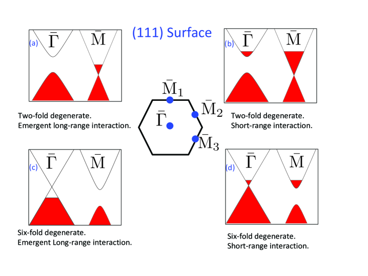
Figure 1: Summary of different magnetization behaviors expected for a (111) TCI surface. The expected of dependence on $T_{c}$ on the magnetic impurity concentration $n_{imp}$ will vary linearly or quadratically depending on whether there are short- or long- range spin-gradient interactions in the system. Inset: Locations of Dirac points in the surface Brillouin zone.

Another remarkable aspect of DW’s in these systems are confined, conducting states that they host Martin et al. (2008); Liu et al. (2009); Fang et al. (2014); Jackiw and Rebbi (1976); Schaakel (2008). For a uniformly magnetized surface of a TI or a TCI, symmetries broken by this (time-reversal in the former, crystal symmetry in the latter) generically induce a Berry’s curvature in the vicinity of a surface Dirac point. Importantly, when multiple Dirac points are involved, this will occur for each in which the magnetization opens a gap in the (local) energy spectrum. We will see explicitly for the concrete example of a TCI that integrating the Berry’s curvature in the vicinity of such points yields Chern numbers $\pm 1/2$, so that the change in Chern number going across the DW is always integral. The numerical calculations we present below demonstrate that one may understand the number of conducting modes hosted by a given DW, as well as their chirality, from the change in Chern numbers summed over all the Dirac points on the surface.

The presence of such conducting states in DW’s opens unique opportunities to interrogate them. In principle they can be forced into a system by pinning the direction of magnetization in opposite directions at two ends of a sample at low temperature, or by quenching to low temperature in zero magnetic field, freezing in thermally generated DW’s. The DW’s could then be imaged, for example, via STM spectroscopy on the surface, or detected indirectly by changes in the surface conductivity due to their presence Dhochak et al. (2015); Assaf et al. (2015); Ueda et al. (2015); Tian and et al. (2016). DW contributions to the dynamical conductivity might also be detected via reflectance measurements from the surface. Such measurements could also afford a window on thermal disordering of the surface magnetism, at which point the DW’s should proliferate. While we expect the longest wavelength critical fluctuations as one approaches thermal disordering to have a character consistent with short-range gradient interactions not (b); Sachdev (2002); Voj , there should exist a crossover regime in which the DW lengths and widths are impacted by the emergent long-range interactions. The existence of DW in-gap states thus introduces a signal of the DW statistics that is measurable in probes coupling to the surface electrons. In this way, domain walls allow, in principle, direct access to the interesting physics that emerges when magnetic degrees of freedom are introduced at TI and TCI surfaces.

This article is organized as follows. We begin in Section II by considering a simple Dirac electron model coupled to a static magnetization, and compute the energy cost coming from introducing gradients in the latter, with rather different behavior resulting when the Fermi energy is at or away from the Dirac point. A related analysis for graphene is presented which yields results consistent with this, and we check this behavior numerically to demonstrate that the physics remains valid in a tight-binding model. We then turn in Section III to energetic calculations of DW pairs, in which we demonstrate the presence of an emergent logarithmic interaction that appears as the magnitude of the magnetization gets small. Two analyses are presented. The first involves a transfer matrix method for a continuum model of Dirac electrons analyzed with a phase shift method, where one finds that the behavior emerges from a near cancellation of the DW separation dependence of the bound state energies, and the remaining spectral dependence found in phase shifts of unbound electrons scattered by the DW’s. This is followed by a numerical analysis of a tight-binding “gapped graphene” model that supports the result, demonstrating again the consistency of continuum and microscopic models. We then turn our attention to a more detailed study of DW’s in a TCI model in Section IV. We begin with an outline of how we model these numerically, in particular explaining a technique for projecting the Hilbert space into a set of surface states that allows us to focus on the effects of magnetic moments near the surface. We then apply this method to compute the Berry’s curvature and Chern numbers in the vicinity of surface Dirac points which become gapped in the presence of a uniform magnetization. This provides us with general expectations for the number and chirality of states appearing in these gaps when there are DW’s. We then explain a method for numerically modeling DW’s in this system, and present results for several realizations of DW’s. In all cases we find that the number and chirality of bound states within them are well-explained by the general expectations arising from our Chern number calculations. We also use this numerical method to demonstrate that in the six-state TCI system, the lowest energy DW’s are generically those that connect groundstates that are closest in orientation. This means that the system is best described as a six-state clock model, rather than two sets of three states separated by a larger barrier. Finally, in Section V we summarize our results, provide further discussion of their significance, and possibilities for further exploration.

II Magnetization Gradient Energy

As discussed above, the unusual behavior of magnetic impurities coupled by Dirac electrons is manifest when one introduces gradients in the magnetization. In this section we demonstrate this within two models of such systems. The first is a simple model for electrons in a surface system where spin-orbit interactions are important, in which the electron wavefunctions involve two components, and the electron spin degree of freedom is projected into these components. These models arise in the context of TI’s and TCI’s Efimkin and Galitski (2014); Reja et al. (2017). The second system we consider is graphene, for which spin-orbit coupling is negligible. The wavefunctions describe amplitudes for electrons to be present on one of two sublattices of the carbon honeycomb structure, with either spin up or down, and are thus four-component. While in real systems the impurities are randomly located so that disorder is present in the system, the relatively long-range of the effective spin-spin interactions when $k_{F}$ is small or vanishing suggests one can coarse-grain the magnetization field over a large area so that disorder effects become small, at least at long wavelengths Efimkin and Galitski (2014); Reja et al. (2017). For simplicity we will ignore the effects of disorder in our analyses.

The underlying coupling between the impurity moments and the electron spin in these models is the $sd$ Hamiltonian, $H_{sd}=J\sum_{i}{\bf S_{i}}\cdot{\bf s}({\bf r}_{i})$, where ${\bf S}_{i}$ is a spin degree of freedom localized at position ${\bf r}_{i}$, and ${\bf s}({\bf r})$ is the conduction electron spin field Yosida (1996). These degrees of freedom may be deposited on the surface of the material, but for TI’s and TCI’s they may be present in the bulk as well. In the latter case, provided the Fermi energy of the system is in the bulk gap, coupling among the bulk impurities will be exceedingly small, so that we expect them to be disordered and for this reason negligible Rosenberg and Franz (2012); Lasia and Brey (2012). The spin impurities are however coupled near the surface where conduction electrons are present. Such models have the attractive feature that the impurity atoms tend to enter as substitutional impurities at the same type of lattice site throughout the crystal, so that there is considerable uniformity in the local coupling between spins and conduction electrons Reja et al. (2017).

II.1 Spin-Orbit Coupled Systems

The coarse-graining approximation described above leads to a continuum form for the coupling Hamiltonian, $H_{sd}\rightarrow\tilde{J}\int d^{2}r{\bf S}({\bf r})\cdot{\bf s}({\bf r})$, which then must be projected into the low-energy sector of the electronic Hamiltonian. The latter consists of one or more single particle Dirac Hamiltonians, which with addition of the spin field ${\bf S}$ takes the generic form

$$H=v_{F}\left\{(-i{{\partial}\over{\partial x}}-b_{y})\sigma_{1}+(-i{{\partial}\over{\partial y}}-b_{x})\sigma_{2}+b_{z}\sigma_{3}\right\},$$ (2)

where we have set $\hbar=1$, as we will throughout this paper, except where otherwise noted. In this expression, $\sigma_{i}$, $i=1,2,3$ are the Pauli spin matrices, $v_{F}$ is the electron speed, and the components of ${\bf b}({\bf r})$ are proportional to projections of ${\bf S}({\bf r})$ onto certain directions. For example, for TI systems $b_{3}$ is proportional to the component of ${\bf S}$ perpendicular to surface Liu et al. (2010); Silvestrov et al. (2012); Efimkin and Galitski (2014); Brey and Fertig (2014). In (Sn/Pb)Te-type TCI systems, it is proportional to the spin component along a particular $\Gamma$-$L$ direction in the bulk band structure Reja et al. (2017). Note that more generally, the electron speeds along the $\hat{x}$ and $\hat{y}$ directions in the plane of the surface may be different, but as this introduces no qualitative effects we ignore it for simplicity.

Our goal is to assess the cost in energy to the system when there is a spatial oscillation in ${\bf b}$ with some wavevector ${\bf Q}$, and we proceed to do this in perturbation theory. For uniform ${\bf b}$, this Hamiltonian has the spectrum $\pm\varepsilon_{0}(q_{x}-b_{y},q_{y}-b_{x})=\pm v_{F}\sqrt{(q_{x}-b_{y})^{2}+(q_{y}-b_{x})^{2}+b_{z}^{2}}.$ To this uniform ${\bf b}$ we add a small oscillatory component $\delta{\bf b}$ with some definite wavevector ${\bf Q}$, so that ${\bf b}=b_{z}\hat{z}+\delta{\bf b}\cos{{\bf Q}\cdot{\bf r}}$. We then compute the change in energy due to $\delta{\bf b}$ in perturbation theory, and examine its Q dependence. Shifting the origin of coordinates in momentum ($q_{x}^{\prime}=q_{x}-b_{2}$, $q_{y}^{\prime}=q_{y}-b_{1}$, with $b_{x}$ and $b_{y}$ the in-plane components of the uniform b-field) eliminates any effect of the uniform $b_{x,y}$ contributions. The single-particle states diagonalizing Eq. 2 then have the form

$$|{\bf q},s\rangle={1\over{\sqrt{\Omega}}}\frac{e^{i{\bf q}\cdot{\bf r}}}{\left[q^{\prime 2}+(s\varepsilon_{0}(q^{\prime})/v_{F}-b_{z})^{2}\right]^{1/2}}\left(\begin{array}[]{c}q_{x}^{\prime}-iq_{y}^{\prime}\\ {s\over v_{F}}\varepsilon_{0}(q^{\prime})-b_{z}\end{array}\right),$$ (3)

where $\Omega$ is the surface area of the system, and $s=\pm 1$ labels the particle- and hole-like states.

II.1.1 Fermi Energy in the Gap

We first consider the situation where the Fermi energy is in the gap of unperturbed energy spectrum. The change in the total energy of electrons is, to leading non-vanishing order,

$$\Delta E=-\sum_{\bf q}\sum_{\bf p}\frac{|\langle{\bf q},-|\delta h|{\bf p},+\rangle|^{2}}{\varepsilon_{0}({\bf q})+\varepsilon_{0}({\bf p})},$$ (4)

where $\delta h=\sum_{i=x,y,z}\delta b_{i}\cos({\bf Q}\cdot{\bf r})\sigma_{i}$, with $\sigma_{i}$ the three Pauli matrices, and we work in units for which $v_{F}=1$. Plugging into Eq. 4 yields

$$\Delta E=-{1\over 4}\sum_{\bf q}\left\{\frac{|\langle{\bf q},-|\delta{\bf b}\cdot{\bf\sigma}|{\bf q}-{\bf Q},+\rangle|^{2}}{\varepsilon_{0}({\bf q})+\varepsilon_{0}({\bf q}-{\bf Q})}+\frac{|\langle{\bf q},-|\delta{\bf b}\cdot{\bf\sigma}|{\bf q}+{\bf Q},+\rangle|^{2}}{\varepsilon_{0}({\bf q})+\varepsilon_{0}({\bf q}+{\bf Q})}\right\}.$$ (5)

Explicit calculations may be carried through with this expression, as we outline in the Appendix. To characterize the quadratic energy cost for magnetization gradients we introduce a tensor quantity $g_{\mu\nu}^{ij}$ by the definition $\Delta E({\bf Q})-\Delta E(0)={{\Omega}\over{2}}\sum_{\mu,\nu=x,y}\sum_{ij=x,y,z}g_{\mu\nu}^{ij}Q_{\mu}Q_{\nu}\delta b_{i}\delta b_{j}$. Many of the $g_{\mu\nu}^{ij}$ coefficients turn out to vanish; the non-vanishing ones are given by

$$g_{xx}^{zz}=g_{yy}^{zz}=2b_{z}^{2}\int\frac{d^{2}q}{(2\pi)^{2}}\frac{q^{2}}{\varepsilon_{0}(q)^{7}}={{8}\over{15\pi b_{z}}}$$ (6)

and

$$g_{xx}^{xx}=g_{yy}^{yy} = \frac{4}{5\pi b_{z}},$$

$$g_{xx}^{yy}=g_{yy}^{xx}=g_{xy}^{xy} = \frac{16}{5\pi b_{z}}.$$ (7)

An important property which must be checked is that the system is stable against gradients of the magnetization, i.e., that the energy of the system can only increase as $Q$ increases from zero. This is manifestly true for gradients associated with $\delta b_{z}$. For the in-plane components, it is convenient to notice that one may write

$$\Delta E({\bf Q})-\Delta E(0)=\left(\begin{array}[]{cc}\delta b_{x}&\delta b_{y}\end{array}\right)\left(\begin{array}[]{cc}g^{xx}_{xx}Q_{x}^{2}+g^{xx}_{yy}Q_{y}^{2}&g^{xy}_{xy}Q_{x}Q_{y}\\ g^{xy}_{xy}Q_{y}Q_{x}&g^{yy}_{xx}Q_{x}^{2}+g^{yy}_{yy}Q_{y}^{2}\end{array}\right)\left(\begin{array}[]{c}\delta b_{x}\\ \delta b_{y}\end{array}\right).$$

Using Eqs. 7, it is easy to confirm that the eigenvalues of the matrix appearing in this equation are always positive for any direction of ${\bf Q}$, and increase quadratically with its magnitude. This indicates that gradients in the magnetization tend to increase the energy of the configuration, so that the spin-spin interactions favor ferromagnetism in this system.

A prominent feature of these results is that all these coefficients diverge as the gap-opening component $b_{z}\rightarrow 0$, indicating a diverging stiffness as the uniform component of the surface magnetization vanishes. On the other hand, if the oscillations in the underlying ${\bf S}$ field come from rotations in the field, but the field itself is of constant length, then we expect $\delta{\bf b}$, $b_{z}$ $\sim|{\bf S}|$, so that $\Delta E({\bf Q})-\Delta E(0)$ is still non-analytic in ${\bf S}$ and is anomalously large when $|{\bf S}|$ is small, but is not divergent in the ${\bf S}\rightarrow 0$ limit.

This surprising result is actually consistent with the effective RKKY spin coupling that is known for graphene; as discussed in the introduction, the $1/R^{3}$ interaction found there leads to long-range gradient interactions, with a Fourier transform that is linear rather than quadratic in $Q$, and hence non-analytic in wavevector. Our perturbative calculation explicitly assumes that $\Delta E({\bf Q})$ is analytic in wavevector, and the divergence of the stiffnesses as $b_{z}\rightarrow 0$ is the signal that this assumption breaks down. To see more clearly how this works, we will consider the energetic cost of imposing a spin gradient on electrons in graphene. Before proceeding with this, however, we extend the analysis discussed above to the case where the electron system is doped, and see that this relieves the large gradient energy found in the calculation above.

II.1.2 Fermi Energy in a Band

When the Fermi energy $\mu$ is alternatively in the band, we end up with a very different result: there is no dependence on the wavevector Q to order $Q^{2}$. Again the perturbation around a uniformly magnetized state will take the form

$$\delta h=\delta{\bf b}\cdot\vec{\sigma}\cos{{\bf Q}\cdot{\bf r}}.$$ (8)

In what follows we assume the Fermi energy $\mu$ is in the valence band – i.e., below the gap. Because the Hamiltonian is particle-hole symmetric we should obtain the same result for $\mu\rightarrow-\mu$. Assuming $Q<\mu$, the change in energy due to the perturbation can be expressed at second order as a sum of two terms, $\Delta E=\Delta E_{+}+\Delta E_{-}$, with

$$\Delta E_{+}={1\over 4}\sum_{\mathclap{\begin{subarray}{c}q>k_{F}\\ |{\bf q}-{\bf Q}|<k_{F}\end{subarray}}}\frac{|\langle{\bf q},-|\delta{\bf b}\cdot\vec{\sigma}|{\bf q}+{\bf Q},-\rangle|^{2}}{\varepsilon_{0}({\bf q}+{\bf Q})-\varepsilon_{0}({\bf q})}-{1\over 4}\sum_{q>k_{F}}\frac{|\langle{\bf q},-|\delta{\bf b}\cdot\vec{\sigma}|{\bf q}+{\bf Q},+\rangle|^{2}}{\varepsilon_{0}({\bf q}+{\bf Q})+\varepsilon_{0}({\bf q})},$$ (9)

where the Fermi wavevector is defined by $\varepsilon_{0}(k_{F})=\mu$. $\Delta E_{-}$ has the same form as Eq. 9, with ${\bf Q}\rightarrow-{\bf Q}$. As demonstrated in the Appendix, when the $\Delta E_{+}$ and $\Delta E_{-}$ are summed, the result is independent of ${\bf Q}$; i.e., the energy required to introduce an oscillation in the magnetization is independent of the oscillation wavevector. This indicates that an effective energy functional for the magnetization should have vanishing coefficient for the quadratic gradient term – effectively, a vanishing spin stiffness. This contrasts dramatically with the situation we found for $\mu=0$, where the stiffness diverged as $b_{z}\rightarrow 0$.

Two comments are in order. The first is that this vanishing stiffness results from the perfect linear spectrum of our unperturbed model. In real systems there is some curvature in the spectrum away from the Dirac point energy, and we expect this will lead to non-vanishing contributions to the stiffness. If the Fermi energy is not too far from the Dirac point then one can treat such deviations perturbatively, and these should be finite. Thus we expect non-vanishing contributions for spin gradients in a doped system, as will be supported by our numerical studies described below, but these will be small compared to what happens when the Fermi energy is in the gap of the uniformly magnetized system. The second is the comparison of this result to a closely related one for graphene: when doped, its spin susceptibility is independent of ${\bf Q}$ for small $Q$ Brey et al. (2007). In this situation, however, RKKY interactions between spins do not vanish, due to contributions from large $Q$. This leads to ferromagnetic coupling among spins on the same sublattice, and antiferromagnetic ones for spins on opposite sublattices, for length scales shorter than $\sim 1/2k_{F}$ Brey et al. (2007). Beyond this scale, the RKKY interactions oscillate and average to zero. The net effect is a short distance coupling, which ultimately leads to a non-vanishing gradient energy for the system..

As we see, the comparison of this system with the behavior of graphene is quite useful, so we next turn to an analysis of what happens in the latter system when a spin gradient is imposed.

II.2 Comparison to Graphene

Because graphene has essentially no spin-orbit coupling, it couples to an impurity spin in a different way than what was examined in the last section. Nevertheless, results for it do bring some insight to systems governed by the Hamiltonian $H$ appearing in Eq. 2. In graphene the spin operator is completely independent of the spinor degree of freedom that $H$ acts upon; spin is a separate quantum number for the electrons. The effect of a single impurity spin is to act like a local Zeeman field with direction fixed by the impurity spin itself.

II.2.1 Perturbation Theory

In the standard perturbative approach to RKKY interactions Ketterson (2016), one computes the static linear spin response $\chi^{ij}_{\alpha\beta}(Q)$ of (the Fourier transform of) the electron spin components $s_{i}({\bf Q})$ to a perturbation $JS_{j}({\bf Q})$, where $J$ is the $sd$ coupling and $\alpha,\beta$ = A,B are indices specifying the sublattice(s) to which the impurities are coupled. The spin symmetry dictates that the spin response has the form $\chi^{ij}_{\alpha\beta}(Q)=\chi_{\alpha\beta}^{0}\delta_{ij}$, and the total change of energy at second order in $J$ is $\Delta E=-J^{2}\sum_{\bf Q}\sum_{i=x,y,z}\sum_{\alpha,\beta}\chi^{0}_{\alpha\beta}(Q)S_{i,\alpha}(-{\bf Q})S_{i,\beta}({\bf Q})$, where $S_{i,\alpha}$ is the $i$th component of the impurity spin field on sublattice $\alpha$.

As has been shown previously Brey et al. (2007), for undoped graphene $\chi_{\alpha\beta}^{0}(Q)$ begins at a positive cutoff-dependent constant for $Q=0$ and varies linearly with increasing $Q$: for example, $\chi_{AA}^{0}(Q)={1\over{4\pi}}\left(\Lambda-{\pi\over 8}Q\right)$, where $\Lambda$ is an upper cutoff of order the bandwidth. For doped graphene $\chi_{AA}^{0}(Q)$ is independent of $Q$ (and equal to the $Q=0$ value for the undoped case) up to $Q=2k_{F}$, where a non-vanishing slope in $Q$ sets in. ($\chi_{AB}$ has the same magnitude as $\chi_{AA}$ but has opposite sign.) The cusp is a realization of the well-known Kohn anomaly and leads to $2k_{F}$ oscillations in the response.

The results are reminiscent of what we found in the last two subsections. The linear behavior in $Q$ for undoped graphene is non-analytic and indicates that the quadratic small $Q$ calculation carried out above must fail in the limit that the gap closes i.e., for vanishing uniform magnetization in the zero-doped, spin-orbit coupled model. Indeed we expect that for ${b_{z}}\rightarrow 0$ that the spin-response associated with Eq. 2 will tend to a combination of $\chi_{AA}^{0}$ and $\chi_{AB}^{0}$ for graphene. Thus, we should understand the divergences in Section II.1.1 in this limit as indicating a crossover from quadratic to linear behavior in the spin response with respect to $Q$ when the system exits the broken symmetry state.

II.2.2 Beyond Perturbation Theory: Helicity Modulus

In contrast to the models considered above, in graphene the expected ordering at low temperature is antiferromagnetic across the sublattices Brey et al. (2007). When this is present the RKKY interaction as calculated perturbatively fails at the longest length scales in a way very analogous to what happened in the spin-orbit coupled case. This occurs because a uniform staggered magnetization acts as a mass term in the Hamiltonian for each spin individually, opening a gap $\Delta$ in the spectrum. If one works perturbatively around this state, one expects an exponential falloff in the spin-spin interaction at length scales beyond that set by $\Delta$. Interestingly, since spin-orbit coupling is essentially negligible in this system, no spin orientation is favored, and it is possible to assess the energetics of spin gradients of different length scales, as we now show.

Suppose the staggered magnetization is characterized by an ordering vector ${\bf b}({\bf r})$. For a square system of linear size $L$ one can imagine a configuration in which ${\bf b}$ rotates precisely once around some fixed axis as ${\bf r}$ varies down the entire length of the sample in some direction. The helicity modulus Chaikin and Lubensky (1995) is defined in terms of the energy cost to introduce this spin twist, relative to a uniform groundstate:

$$\rho_{s}(g=2\pi/L)=\lim_{L\rightarrow\infty}2L^{-2}\left[E(g=2\pi/L)-E(g=0)\right]/(2\pi)^{2},$$ (10)

where $g$ is the wavevector of the imposed spin gradient, and $E(g)$ is the energy of the system (proportional to its area) with some imposed spin gradient. While $\rho_{s}(g=0)$ is the spin stiffness of the system at the longest possible length scale available in a finite size system, we can generalize this quantity by allowing $g$ to be a free variable, probing the energy cost for gradients at length scales $2\pi/g$. This quantity may be computed for graphene subject to a uniformly rotating staggered magnetization.

Our Hamiltonian in this situation is

$$H_{G}=v_{F}\left[\hat{p}_{x}\tau_{x}+\hat{p}_{y}\tau_{y}-{\bf b}\cdot{\vec{\sigma}}\tau_{z}\right],$$ (11)

where $\vec{\sigma}$ is the set of Pauli matrices acting on the spin degree of freedom, $\vec{\tau}$ are the corresponding matrices acting in the sublattice space, and $\hat{p}_{x,y}$ are components of the momentum operator. As above we set $v_{F}=1$. If ${\bf b}={b}_{0}(\sin\theta,0,\cos\theta)$ is independent of position, then the eigenstates of ${\bf b}\cdot\vec{\sigma}$ are

$$\chi_{+}=\left(\begin{array}[]{c}\cos\frac{\theta}{2}\\ \sin\frac{\theta}{2}\end{array}\right), \quad\chi_{-}=\left(\begin{array}[]{c}-\sin\frac{\theta}{2}\\ \cos\frac{\theta}{2}\end{array}\right),$$ (14)

and the corresponding eigenergies of $H_{G}$ are given by $\pm\sqrt{p_{x}^{2}+p_{y}^{2}+b_{0}^{2}}$, each of which is two-fold degenerate. To compute $\rho_{s}(g)$ we will need to find the single-particle energies in the situation where $\theta\rightarrow gx$. To do this we transform our spin quantization axis to be locally parallel to ${\bf b}(x)$. This is equivalent to writing the eigenstates of Eq. 11 in the form

$$\Psi(x)={\mathbf{\alpha}}(x)\otimes{\bf\chi}_{+}(x)+{\mathbf{\beta}}(x)\otimes{\bf\chi}_{-}(x),$$ (15)

where the $\sigma$ matrices act on the vectors ${\bf\chi}_{\pm}$, and the $\tau$ matrices act on the two-component vectors ${\mathbf{\alpha}}$ and ${\mathbf{\beta}}$. With some algebra, one can show that the stationary state equation $H_{G}\Psi=\varepsilon\Psi$ can be cast in the form

$$(\tilde{H}-\varepsilon)\left(\begin{array}[]{c}{\mathbf{\alpha}}\\ \mathbf{\beta}\end{array}\right)=0,$$ (16)

where

$$\tilde{H}=p_{x}\tau_{x}+p_{y}\tau_{y}-b_{0}\tau_{z}\mu_{x}-g\mu_{z}\tau_{x},$$ (17)

and the $\vec{\mu}$ Pauli matrices act in the $(\alpha,\beta)$ space.

The solutions to Eq. 16 can be evaluated directly, yielding four single particle energies,

$$\pm{\varepsilon}_{s}({\bf p})=\pm\left\{p^{2}+g^{2}+b_{0}^{2}+2sg\sqrt{p_{x}^{2}+b_{0}^{2}}\right\}^{1/2},$$ (18)

where $s=\pm 1$. We are interested in the situation where the negative energy states are completely full, so the total energy is

$$E(g)=-\sum_{s}\sum_{{\bf p}}{\varepsilon}_{s}({\bf p}).$$ (19)

From this we wish to subtract the energy at $g=0$. The single particle energies of the filled states are clearly $-\sqrt{p^{2}+b_{0}^{2}}\equiv-\varepsilon_{0}({\bf p})$. The energy difference $E(g)-E(0)$ can be written in the form

$$\Delta E(g)\equiv E(g)-E(0)=-\sum_{p}\left[\varepsilon_{+1}({\bf p})+\varepsilon_{-1}({\bf p})-\varepsilon_{0}({\bf p}-g\hat{x})-\varepsilon_{0}({\bf p}+g\hat{x})\right].$$ (20)

The shift of the $g=0$ energies in the subtraction does not affect the result provided the system obeys periodic boundary conditions, and in this form one may confirm that the sum over ${\bf p}$ in Eq. 20 is independent of cutoff. Substitution yields the explicit expression

$$\Delta E(g) = -\sum_{{\bf p}}\Biggl{\{}\left[p^{2}+b_{0}^{2}+2g\sqrt{p_{x}^{2}+b_{0}^{2}}+g^{2}\right]^{1/2}+\left[p^{2}+b_{0}^{2}-2g\sqrt{p_{x}^{2}+b_{0}^{2}}+g^{2}\right]^{1/2}$$ (21)

$$- \left[p^{2}+b_{0}^{2}+2gp_{x}+g^{2}\right]^{1/2}-\left[p^{2}+b_{0}^{2}-2gp_{x}+g^{2}\right]^{1/2}\Biggr{\}}.$$

Assuming the system to be of sizes $L_{x}$ and $L_{y}$ in the $\hat{x}$ and $\hat{y}$ directions respectively we can replace the momentum sum in the thermodynamic limit by an integral. If we assume $g<<b_{0}$, to lowest non-trivial order in $g$ we find

$$\Delta E(g)\approx L_{x}L_{y}g^{2}b_{0}^{2}\int\frac{d^{2}p}{(2\pi)^{2}}\frac{1}{\varepsilon_{0}(p)^{3}}\sim L_{x}L_{y}g^{2}b_{0}.$$ (22)

The result is anomalous in the sense that, for a generic magnet where the stiffness usually depends analytically on the magnetization scale, we expect $\rho_{s}\sim L_{x}L_{y}\Delta E(g)\sim b_{0}^{2}g^{2}$. Eq. 22 is consistent with a long-range interaction among spin gradients that is cut off by the scale of the magnetization itself, $b_{0}$. This interpretation is further supported by considering larger values of $g$. To do this, we compute the $p_{y}$ integral in $\Delta E(g)$ analytically, which allows it to be cast in the form $\Delta E(g)=-L_{x}L_{y}\frac{g^{3}}{(2\pi)^{2}}G(\frac{b_{0}}{g})$, with

$$G(u)\equiv\int_{-\infty}^{\infty} dx \Biggl{\{}\left[1+u^{2}+x^{2}\right]\log\left[\frac{(1+u^{2}+x^{2})^{2}-4x^{2}}{(1-u^{2}-x^{2})^{2}}\right]$$ (23)

$$+ 2x\log\left[\frac{1+2x+x^{2}+u^{2}}{1+2x+x^{2}+u^{2}}\right]$$

$$- 2\sqrt{x^{2}+u^{2}}\log\left|\frac{1+\sqrt{x^{2}+u^{2}}}{1-\sqrt{x^{2}+u^{2}}}\right|\Biggr{\}}.$$

Note in writing this expression we have taken the momentum cutoff to infinity. One may compute $G(u)$ numerically, with the result that $G(u)\sim-u^{2}$ for $u<<1$, and $G(u)\sim-|u|$ for $u>>1$, as illustrated in Fig. 2. The latter result reproduces the explicit small $g$ result, while the former shows $\Delta E(g)\sim b_{0}^{2}|g|$ for $b_{0}<<g$. This non-analytic behavior in $g$ is what one expects from the linear $Q$ behavior of the spin susceptibility discussed in the previous subsection, indicative of long-range interaction for magnetization gradients. We see however that the interaction is cutoff by the average magnetization $b_{0}$. This length scale can become very large in the limit of low magnetic impurity density or a relatively small $sd$ coupling scale $J$.

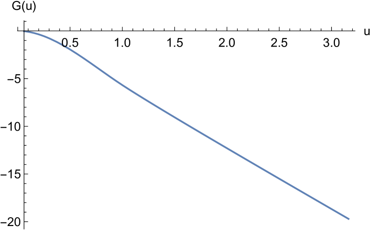
Figure 2: Numerical result for $G(u)$ (Eq. 23) as a function of $u$.

The result holds as well for graphene when treated in the tight-binding model. To show this, we consider the simplest such system in which the carbon atoms are laid out in a triangular lattice with two atoms per unit cell and lattice parameter $a$, with nearest neighbor hopping $t$. The Fermi velocity is related to the tight-binding parameters via $\hbar v_{F}=\sqrt{3}/2ta_{0}$. In each unit cell there is an effective Zeeman energy ${\bf h}=\Delta\hat{z}$, in opposite directions for each of the sublattices, modeling the staggered magnetization. We consider a ribbon of this, with cross-sectional width $L_{w}$, in which ${\bf h}$ rotates around an axis by $2\pi$ along the ribbon cross-section. The system has well-defined momentum along the $\hat{y}$-direction, $p_{y}$, and for each of these we compute a set of single-particle energies by diagonalizing the tight-binding model numerically. The relevant electronic energy of the system is the sum of all negative energy states, integrated (numerically) over $p_{y}$. From this we subtract the corresponding energy for a uniform staggered magnetization ${\bf h}$, with the same magnitude $\Delta$. This difference is $\Delta E(g=2\pi/L_{w})$. When $v_{F}/L_{w}\gg\Delta$, one expects $\Delta E\sim L_{w}g$ becomes constant as $L_{w}$ grows. By contrast, for fixed $L_{w}$ it should grow linearly with increasing $\Delta$. This behavior is consistent with the numerical observations, as illustrated in Fig. 3.

II.3 Discussion

We conclude this section with some observations as well as speculations regarding the impact of the unusual gradient energy in these systems. In the context of DW’s, one interesting consequence is how the energetics impacts the temperature at which the system should disorder. A simple estimate Vanderzande (1998); Shankar (2017) of the free energy to create a DW of length $L$ against an otherwise uniform magnetization background takes the form $\Delta F(L)=\varepsilon L-k_{B}T\eta(L/\xi)$, where $\varepsilon\sim\sqrt{\rho_{s}\bar{S}}$ is the energy per unit length, with $\bar{S}$ the average magnetization per unit area, and $\xi\sim\sqrt{\rho_{s}/\bar{S}}$ is the width of a DW, $T$ is the temperature, and $\eta$ is factor of order unity which characterizes how quickly the DW changes its direction as one moves down its length, in units of $\xi$; the second (entropic) term arises from the number of configurations one may construct for the DW, in which the complicating factors of interactions among different parts of the DW have been ignored, as well as the fact that a finite $L$ DW in a system without boundaries is actually a closed loop. In spite of these simplifications, for the Ising model the condition $\Delta F(L)<0$, which is interpreted as DW proliferation and the loss of magnetic order in the system, yields an estimate of $k_{B}T_{c}=\varepsilon\xi/a\sim\rho_{s}$. In the Ising model, this type of argument yields the correct $T_{c}$ to within 25% of the exact answer Shankar (2017).

In the present system, however, the behavior of $\rho_{s}$ is anomalous. For example, for short-range interactions this scales as $\rho_{s}\sim\bar{S}^{2}$, which in turn is proportional to the square of the impurity density, since the $\rho_{s}$ is a long-wavelength measure of interactions among the impurities. If one uses the long wavelength estimate for systems analyzed above, we find $\rho_{s}\sim\bar{S}$, linearly proportional to the impurity density. This behavior contrasts with what happens when the Fermi energy is moved away from any Dirac point energy of the surface, in which case we return to a magnetic system with short-range interactions: $T_{c}$ then scales quadratically with impurity density. This change in behavior is an in-principle measurable signature of the interesting DW energetics in these systems.

In addition to the anomalous average magnetization dependence of DW’s in this system, our gradient analysis suggests an emergent long-range interaction which becomes important at increasingly long length-scales as the magnetization decreases. In the next section, we will demonstrate the presence of this interaction by examining the energetics of inter-DW interactions.

III Domain Wall Interactions

As discussed above, one aspect of the unusual gradient interactions in these systems would be the emergence of long-range interactions between DW’s as the magnetization scale gets small. To test this, we will compute these interactions directly in two simple models: continuum Dirac electrons coupled to a piecewise constant magnetization field, and a tight-binding model of “gapped graphene.” In both cases we will see that the character of the interaction changes significantly depending on the placement of the chemical potential $\mu$: when it passes through the magnetization-induced gap, it becomes increasingly long-ranged as the magnetization becomes small. When $\mu$ is outside this gap, the interaction remains short-ranged even as the gap closes.

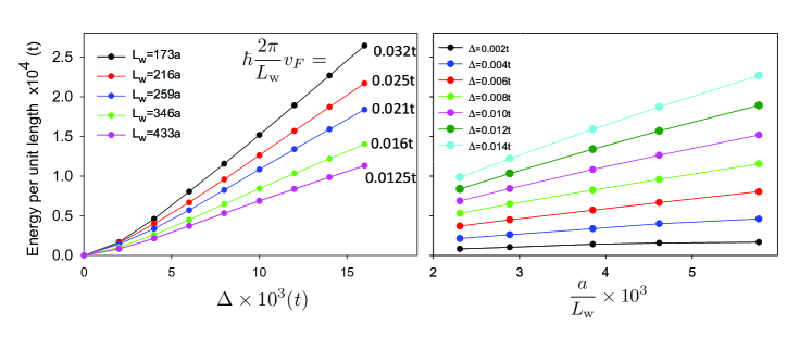
Figure 3: Numerical calculation of energy per unit length required for single overturn of the staggered magnetization $\Delta$ in a graphene ribbon of width $L_{w}$, relative to that with a uniform staggered magnetization, for various values of $L_{w}$ and $\Delta$. When $L_{w}$ is held fixed, this energy grows linearly with $\Delta$. For fixed $\Delta$, the energy approaches a constant as $1/L_{w}$ grows.

III.1 Continuum System with Piecewise Constant Magnetization: Phase Shift Analysis

We begin with a generic surface Dirac Hamiltonian of the form in Eq. 2, which within regions of constant magnetization may be written as

$$H=(k_{y}-b_{y})\sigma_{x}+(k_{x}-b_{x})\sigma_{y}+\Delta\sigma_{z},$$ (24)

where $k_{x}$ and $k_{y}$ are components of the electron wavevector for the system surface with constant magnetization. In this equation we have taken our unit of energy to be $\hbar v_{F}/a_{0}$, where $v_{F}$ is the speed associated with the Dirac point when $\Delta=0$, and our length unit $a_{0}$ is set by a microscopic lattice scale. Our approach will be to consider linear combinations of the eigenstates associated with this type of Hamiltonian, matching them across boundaries where $b_{x}$, $b_{y}$, and $\Delta$ change suddenly. We compute a transfer matrix for the system, from which we can obtain both bound state energies and phase shifts for scattered states, allowing us to compute the energies of each of these as a function of separation between two DW’s. We will see the effects of these combine in a surprising way to yield a slow variation of the system energy when the chemical potential is in the gap, and the separation is not too large.

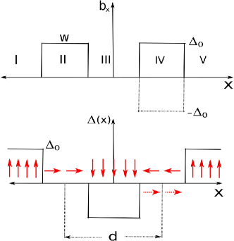
Figure 4: Piecewise constant domain wall configuration with two domain walls of width $w$ each separated by a center-to-center distance $d$. Top panel: The parameter $b_{x}$, for which we allow the possibility of values that are equal or opposite, allowing for magnetizations that rotate with the same or with opposite senses. Piecewise constant regions $I-V$ are labeled. Bottom panel: $\Delta(x)$, illustrating that the magnetization rotates from up to down and back again. Arrows indicate the orientation of the magnetization vector in each region.

III.1.1 Wavefunctions

The type of DW configuations we analyze are illustrated in Fig. 4, which contain five separate regions in which $\Delta$ and $b_{x}$ are constant, labeled $I$ through $V$. The rotation of the magnetization within the two DW’s may have the same or opposite senses, as illustrated by the solid and dashed arrows in Region $IV$. We treat this as a scattering problem where electrons in regions $I$ and $V$ are connected through a transfer matrix $T$,

$$\vec{\Psi}_{V}=T\vec{\Psi}_{I}$$ (25)

The two components of the wavefunctions $\vec{\Psi}_{i}$ represent amplitudes for the two orbitals upon which the Dirac matrices in Eq. 24 act. To obtain the transfer matrix $T$, we find eigenvectors of this Hamiltonian for some fixed energy $E$ in each region, and match both components of the wave functions at each boundary ($I$ to $II$, $II$ to $III$, etc.) Note that $k_{y}$ is a good quantum number and is constant for a wavefunction in all regions.

The general form for the wavefunction in region $j$ may be written as

$$\vec{\Psi}_{j}=e^{ik_{y}y}\left[A_{j}e^{i(k_{x}^{+})_{j}x}\left(\begin{array}[]{c}u_{+}^{j}\\ v_{+}^{j}\end{array}\right)+B_{j}e^{i(k_{x}^{-})_{j}x}\left(\begin{array}[]{c}u_{-}^{j}\\ v_{-}^{j}\end{array}\right)\right],$$ (26)

and energy $E=-\sqrt{k_{y}^{2}+k_{x}^{2}+\Delta_{0}^{2}}$ the same in all regions. We solve this straightforwardly to obtain the values of $k_{x}$ for the scattering states in regions $I$ and $V$; note for bound states this may turn out be imaginary. The energy also determines the values of $(k_{x}^{\pm})_{j}$ in each of the “internal” regions $j=II,III,IV$,

$$(k_{x}^{\pm})_{j}=-b_{x}^{j}\pm\sqrt{E^{2}-k_{y}^{2}-\Delta_{j}^{2}}.$$ (27)

In terms of these the values of $u,v$ are given by

$$u_{\pm}^{j}=\frac{k_{y}-i((k_{x}^{\pm})_{j}+b_{x}^{j})}{\sqrt{(\Delta_{j}-E)^{2}+k_{y}^{2}+((k_{x}^{\pm})_{j}+b_{x}^{j})^{2}}},$$

$$v_{\pm}^{j}=\frac{E-\Delta_{j}}{\sqrt{(\Delta_{j}-E)^{2}+k_{y}^{2}+((k_{x}^{\pm})_{j}+b_{x}^{j})^{2}}}.$$

With this information, the $T$ matrix may be straightforwardly computed analytically; the expression is lengthy and we do not present it explicitly. Note that the $T$ matrix contains the information about the domain wall width $w$ and the distance $d$ between the two domain walls (DWs). We will compute the energy of the DW structure from $T$, which contains two contributions of similar size, one from bound states induced by the DW’s, and one from scattering phase shifts.

III.1.2 Energy from Bound States

We can express the scattering amplitudes in terms of the components of $T$ using

$$A_{V}=T_{AA}A_{I}+T_{AB}B_{I},B_{V}=T_{BA}A_{I}+T_{BB}B_{I},$$ (28)

where $A$ and $B$ are the amplitudes for right- and left- moving electrons, respectively, in the $I$ and $V$ regions. To obtained the bound state solution, we put $k_{x}\rightarrow i\kappa$ and find $\kappa$ such that $A_{I}=B_{V}=0$. This condition is satisfied when $T_{BB}=0$.

For a given $w$ and $d$, we numerically find the solution for $\kappa$ which gives $T_{BB}=0$. A very nice simplification for this particular geometry is that the solution is independent of $k_{y}$, which makes the computation of this energy contribution particularly simple, once $\kappa$ is known. Since the model we are considering is particle-hole symmetric, we need only consider chemical potentials $\mu\leq 0$. The total energy contribution from the bound states is given by summing over all states with energy below $\mu$, which includes only negative energy states,

$$\Delta E_{b}/L_{y}=-\frac{1}{\pi}\int_{k_{y}^{c}}^{\pi}dk_{y}\sqrt{k_{y}^{2}+\Delta_{0}^{2}-\kappa^{2}},$$ (29)

where $L_{y}$ is the length of the system along the $\hat{y}$ direction. Note the lower cutoff $k_{y}^{c}$, which is given by

$$k_{y}^{c}=\begin{cases}\sqrt{\mu^{2}-\Delta_{0}^{2}+\kappa^{2}}&\text{if $(\mu^{2}-\Delta_{0}^{2}+\kappa^{2})\geq 0$,}\\ 0&\text{otherwise,}\end{cases}$$

is non-trivial because a bound state will only be present below a given $\mu$ if $k_{y}$ is sufficiently large. The integral in Eq. 29 is straightforward to compute with the numerically generated values of $\kappa$.

III.1.3 Energy from Scattering States

We next need to calculate the change in electronic energy due phase shifts of the wave functions due to scattering from the DWs. To do this we imagine the whole system to be embedded at the center of a large box of length $L$, whose size we will eventually take to infinity. For simplicity we require the lower component of the wave function to vanish at the edges of this box. (Other boundary conditions may be considered but should not have qualitative effects on the results.) Using Eqs. 25 and 26, this leads to a condition for the allowed states in this box,

$$\frac{T_{AA}e^{ik_{x}L}-T_{AB}}{T_{BB}e^{-ik_{x}L}-T_{BA}}=1.$$ (30)

This may be rewritten as a quadratic equation for $e^{ik_{x}L}$ in terms of the matrix elements of $T$, whose solutions we cast in the form $e^{ik_{x}L}=e^{iq_{n}L+i\eta_{\pm}(k_{x})}\equiv e^{ik^{\prime}L}$. The values of $\eta_{\pm}(k_{x})$ give allowed values of $k_{x}L$, with the $\eta_{+}$ solutions corresponding to $q_{n}\equiv n\pi/L$, with $n$ the even positive integers, when the DWs are eliminated ($T\rightarrow$ unity), and with $\eta_{-}$ corresponding to $q_{n}$ with $n$ odd in the same limit. Interestingly, we again find a useful independence from $k_{y}$: for a given $k_{x}$ the total phase shift $\eta(k_{x})=\eta_{+}(k_{x})+\eta_{-}(k_{x})$ is independent of $k_{y}$. The shift in energy due to the DW structure comes from the differences between $q_{n}$ and $k^{\prime}(q_{n})$, which, though small, add up to a finite contribution when summed over all the occupied states. To see this one starts with the expression for the total energy contribution due to the scattering states,

$$E_{ph}/L_{y}=\int{{dk_{y}}\over{2\pi}}\sum_{n,\,filled}E[k_{x}(q_{n}),k_{y}].$$

For large $L$, we recast the sum over $n$ as a momentum integral,

$$E_{ph}^{\pm}/L_{y}\rightarrow\int{{dk_{y}}\over{2\pi}}\int{{Ldq}\over{2\pi}}E[k_{x}(q),k_{y}].$$

Here $\pm$ corresponds to the two solutions for the phase shift, $\eta_{\pm}(k_{x})$. Now using the relation $k_{x}L=q_{n}L+\eta_{\pm}(k_{x})$, the energy may be written as

$$E_{ph}^{\pm}/L_{y}=\int{{dk_{y}}\over{2\pi}}\int\frac{dk_{x}}{2\pi}(L-\frac{d\eta_{\pm}(k_{x})}{dk_{x}})E[k_{x},k_{y}].$$

The first term gives a constant background which is independent of the DW separation, and so maybe ignored. Adding the non-trivial contributions from $\eta_{+}$ and $\eta_{-}$, we obtain the energy increase due to scattering,

$$\frac{\Delta E_{ph}}{L_{y}}=-\frac{1}{4\pi^{2}}\int\int dk_{y}dk_{x}\frac{d\eta(k_{x})}{dk_{x}}E[k_{x},k_{y}].$$

As mentioned above, the total phase shift $\eta(k_{x})$ is independence of $k_{y}$, so we may rewrite the above equation as

$$\frac{\Delta E_{ph}}{L_{y}}=-\frac{1}{4\pi^{2}}\int dk_{x}\frac{d\eta(k_{x})}{dk_{x}}\int dk_{y}E[k_{x},k_{y}].$$

Note that the domain of integration for $k_{x},k_{y}$ must respect the condition $E[k_{x},k_{y}]<-|\mu|$. When the chemical potential is in the gap for the uniformly magnetized system, both $k_{x}$ and $k_{y}$ will vary from $-\pi/a_{0}$ to $\pi/a_{0}$ for some cutoff scale $\Lambda=\pi/a_{0}$.

Since our analysis above yields explicit expressions for $\eta(k_{x})$ (again, not presented as this is lengthy yet straightforward to obtain), it is convenient to integrate this directly rather than its derivative. Up to surface terms which are independent of the DW separation, partial integration yields

$$\frac{\Delta E_{ph}}{L_{y}}=-\frac{1}{2\pi^{2}}\int_{0}^{\pi/a_{0}}dk_{x}\eta(k_{x})\frac{dF(k_{x})}{dk_{x}}$$ (31)

where $F(k_{x})$ is given by

$$F(k_{x})=\int_{k_{y}^{c}}^{\pi/a_{0}}dk_{y}\sqrt{k_{x}^{2}+k_{y}^{2}+\Delta_{0}^{2}}.$$ (32)

The lower limit $k_{y}^{c}$ is again defined as

$$k_{y}^{c}=\begin{cases}\sqrt{\mu^{2}-\Delta_{0}^{2}-k_{x}^{2}}&\text{if $(\mu^{2}-\Delta_{0}^{2}-k_{x}^{2})\geq 0$,}\\ 0&\text{otherwise.}\end{cases}$$

The integral in Eq. 31 is straightforward to evaluate numerically.

III.1.4 Results

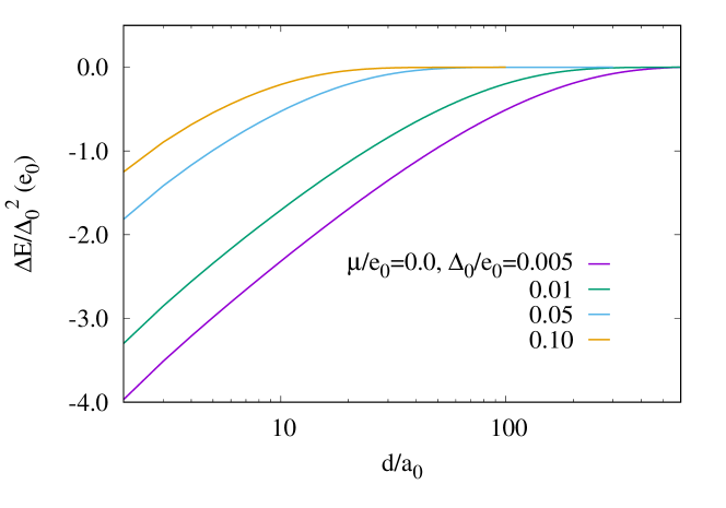
Figure 5: DW pair energy (adding the contributions from both the bound state and phase shift) as a function of the distance between the domain walls $d$ when $\mu$ is in the gap. Different lines indicate different values of $\Delta_{0}$, as indicated. Energies expressed in units of $e_{0}\equiv\hbar v_{F}/a_{0}$.

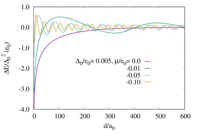
Figure 6: DW pair energy (adding the contributions from both the bound state and phase shift) as a function of the distance between the domain walls $d$ when $\Delta_{0}=0.005$ for various values of $\mu$, as indicated. Energies expressed in units of $e_{0}\equiv\hbar v_{F}/a_{0}$.

We next turn to a discussion of results from this analysis. In all cases the basic energy scale is set by the square of the gap energy $\Delta_{0}$, which we scale out in presenting the results. Distances are shown in units of the cutoff length scale $a_{0}$, which may be taken for concreteness as the lattice constant of the underlying structure. Fig. 5 illustrates typical results for the energy of a pair of DW’s as a function of their separation, for different values of the gap $\Delta_{0}$ for the uniform magnetization far from the pair, when the chemical potential $\mu$ is in the gap. In these calculations, the DW widths are taken to be 0 so that the magnetization jumps discontinuously at each DW. The results are shown on a linear-log scale, and it is apparent for the smallest values of $\Delta_{0}$ that the energy rises nearly linearly towards the asymptotic value for well-separated DW’s. This behavior is expected for interactions between spin-gradients that vary as $1/R$, so that the interaction between line-like objects such as a DW will be logarithmic. As expected from our analysis above, this long-range interaction is emergent, in the sense that it is cut-off at a distance scale that diverges as $\Delta_{0}$ vanishes. We find very similar results for finite width DW’s, for both cases where the in-plane spins are parallel or antiparallel (see Fig. 4.) The basic interaction between DW’s is set by the change in gap-opening component of the field, not the components perpendicular to this.

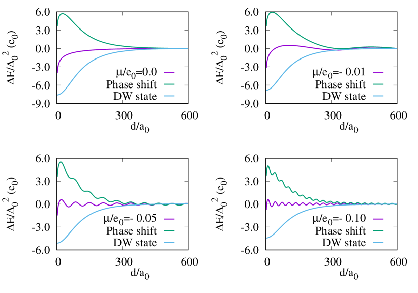
Figure 7: Contributions to DW pair energy from bound states and phase shifts shown separately, for $\Delta_{0}=0.005e_{0}$ and for various values of chemical potential as indicated. Energies expressed in units of $e_{0}\equiv\hbar v_{F}/a_{0}$. The near cancellation of the two contributions is apparent.

Fig. 6 illustrates corresponding results for fixed $\Delta_{0}=0.005$, in units of $\hbar v_{F}/a_{0}$, for different values of $\mu$. Here it makes most sense to present the results on a linear scale, and it is apparent that effective range of the DW attraction shrinks as $\mu$ moves deeper into a band. The expected $2k_{F}$ oscillations are also apparent. Figs. 5 and 6 firmly establish the qualitative differences between DW interactions for $\mu$ in a gap and $\mu$ in a band.

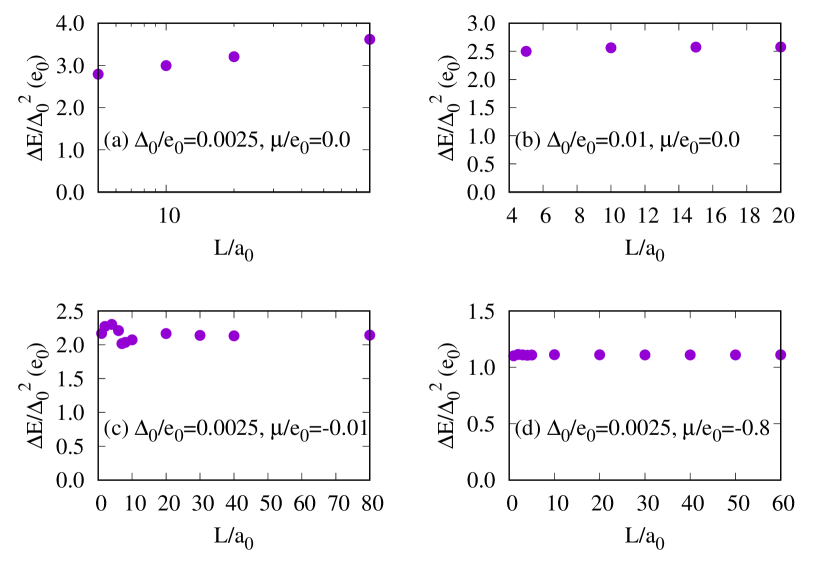
Figure 8: Energy of DW superlattice as a function of separation $L$ for graphene, for different values of $\mu$ and $\Delta_{0}$ as indicated, in energy units of $e_{0}\equiv\hbar v_{F}/a_{0}$. Domain wall are one unit cell wide. Note x-axis is on a log scale in (a), but on a linear scale in the other figures.

As discussed above, these interactions arise from the combined effects of the bound states in the DW’s and the phase shifts of the scattering states.

It is interesting to examine the contributions of these separately, as we do in Fig. 7. Interestingly, one finds an attractive bound state contribution which slightly overbalances a repulsive phase shift contribution, to yield a net attractive interaction. The ranges of each individually turn out to be considerably longer range than the net attraction, and their sums yield the characteristic behaviors illustrated in Figs. 5 and 6. This is a surprisingly intricate way for the slow $d$ dependence of the interaction that emerges at small $\Delta_{0}$ to be realized microscopically: our expectations of its presence descended from perturbative analyses around uniform magnetized systems, which contain no obvious signals that the DW’s will host bound states at all. This behavior is a remarkable demonstration of how the topological character of the underlying bands – which necessitate the presence of the bound states – plays a powerful if subtle role in yielding the long-wavelength physics of the magnetic degrees of freedom in this system.

III.2 A Microscopic Realization: Gapped Graphene

The results in the previous subsection were derived in the context of a continuum model with an imposed short length-scale cutoff. To further establish the presence of the emergent long-range interaction, we wish to see that it is present in a microscopic, i.e., a tight-binding, model. To do this, we consider a model of spinless electrons in a graphene lattice, with a staggered potential that varies in the $\hat{x}$ direction. In general, in such a staggered potential graphene is a normal insulator; however, under certain circumstances it does have a non-trivial topological character. This behavior emerges because each valley carries a half integer Chern number of opposite sign. In geometries for which valleys are not admixed, the system will behave in ways akin to more protected topological systems. For example, when there are regions of opposing staggered potential $\Delta_{0}$ meeting at a valley-preserving interface, valley-dependent gapless chiral modes are known to emerge Xiao et al. (2007); Yao et al. (2009).

The staggered potential we employ in our model has four regions: one with amplitude $\Delta_{0}$, one with amplitude $-\Delta_{0}$, separated by two regions where the staggered potential vanishes for one unit cell along the $\hat{x}$ direction. These two regions are a distance $L$ apart, and model DW’s in the system. The entire system obeys periodic boundary conditions along the $\hat{y}$ direction, and is periodic in the $\hat{x}$ direction up to a phase $e^{ik_{x}(2L+2a)}$, with $a$ the DW width (equivalent to the basic unit cell size in our model). The system may be understood as a superlattice of DW’s, with the total number of DW pairs given by the number of $k_{x}$ values retained in the calculation. A corresponding wavevector $k_{y}$ for the $\hat{y}$-direction is also a good quantum number, and the number of $k_{y}$ values retained effectively fixes the size of the system in this direction. Finally, the microscopic lattice structure is oriented such that the centers of the two valleys (${\bf K}$ and ${\bf K}^{\prime}$ points) are separated along the $\hat{y}$ direction, avoiding valley-mixing effects Brey and Fertig (2006); Palacios et al. (2010).

To assess the energetics of this system, we compute the total electronic energy for negative energy states up to some choice of chemical potential $\mu$, and subtract from this the corresponding energy for a system of the same size with uniform staggered magnetization $\Delta_{0}$. $\mu$ may be chosen to be in the gap or within a band of the latter. Note that the spectrum is particle-hole symmetric, so we only examine non-positive values of $\mu$. This energy difference is a measure of the energy required to create the DW pairs, and by varying $L$ we obtain a measure of their interaction energy.

Fig. 8 illustrates some typical results. In panel (a) we illustrate the DW pair energy as a function of $L$, on a linear-log scale, for a small value of $\Delta_{0}$ and $\mu$ in the gap. The straightness of the line clearly attests to the logarithmic interaction in this distance scale. For large enough $L$ we expect the interaction energy to reach a constant value, and this behavior is demonstrated in panel (b) for larger $\Delta_{0}$, where the asymptotic length scale is not so large that it is difficult to reach numerically. Panels (c) and (d) contrast these with the situation for $\mu$ in a band, where it is clear that the interaction is much shorter in range. Note that the $2k_{F}$ oscillations are not apparent in these figures; this is due to the number of ${\bf k}$ values retained (20 $k_{x}$ values, 1001 $k_{y}$ values) which leads to a relatively small number of bands cutting through the chemical potential. In principle a much larger number of $k_{x}$ values should bring out the oscillations, but in practice we find this requires a smaller number of $k_{y}$ values, which we find sacrifices accuracy at short distances. Thus, although these numerics are limited by the absence of the expected $2k_{F}$ oscillations at long distances, they do confirm the transition from logarithmic to short-range behavior (for small $\Delta_{0}$) as $\mu$ moves into a band.

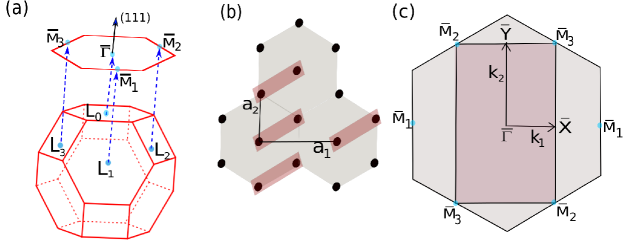
Figure 9: (a) The fcc Brillouin zone containing $L_{i}(i=0,1,2,3)$ points and their projections onto the (111) surface, which yield the $\bar{\Gamma}$ and ${\bar{M}_{i}}(i=1,2,3)$ points. (b) Extended real space unit cells with two atoms per unit cell, used in constructing a domain wall. (c) Surface Brillouin zone for the two surface atom unit cell, which folds the original hexagonal Brillouin zone for the single atom (real space) unit cell into a rectangular one.

IV Domain Walls in TCI Materials

As discussed above, interactions among DW’s in Dirac-mediated systems involves a delicate balance of the energetics of the bound states they host and the scattering of unbound states. Moreover, the possibility of detecting the DW’s is greatly enhanced by the bound states because they render the DW’s conducting. While the analyses discussed above have largely focused on magnetic moments at a surface coupled by a single Dirac point, many systems actually host multiple points, all coupling to the magnetic moments and contributing to the effective interactions among spin gradients. In this last section, we study this in some detail for the interesting case of TCI materials, where the competition among these can lead to multiple orientations for the ground state energy Reja et al. (2017). In particular we will demonstrate that for the (111) surface of TCI’s in the (Sn/Pb)Te class, for a uniform magnetized system each distinct Dirac point has an associated Chern number of $\pm 1/2$, and that the total change of Chern number across a DW correctly predicts the number of states hosted, independent of details of the DW structure. We will also present numerical evidence that the DW energetics strongly suggest that these systems should be described by a six-state model under appropriate circumstances.

IV.1 Tight-Binding Model

TCI’s such as (Pb/Sn)Te have band topology protected by mirror symmetry. The Bravais lattice of the system is fcc with two sublattices (i.e, a rocksalt structure), which we label $a$ and $b$. Focusing on the (111) surfaces, it is convenient to view the structure as two-dimensional triangular lattices with ABC stacking. In this orientation, triangular layers of $a$ and $b$ atoms are arranged alternately along the (111) direction.

A “standard” tight-binding model for these systems is given by Littlewood and et al. (2010); Hsieh et al. (2012) $H_{bulk}=H_{m}+H_{nn}+H_{nnn}+H_{so}$, with

$$H_{m} = \sum_{j}m_{j}\sum_{{\bf R},s}{\bf c}^{\,\,{\dagger}}_{j,s}({\bf R})\cdot{\bf c}_{j,s}({\bf R}),\quad\quad\quad\quad$$

$$H_{nn} = t\sum_{({\bf R},{\bf R^{\prime}}),s}{\bf c}^{\,\,{\dagger}}_{a,s}({\bf R})\cdot{\bf d}_{{\bf R},{\bf R^{\prime}}}{\bf d}_{{\bf R},{\bf R^{\prime}}}\cdot{\bf c}_{b,s}({\bf R^{\prime}})+h.c.,$$

$$H_{nnn} = \sum_{j}t_{j}^{\prime}\sum_{(({\bf R},{\bf R^{\prime}})),s}{\bf c}^{\,\,{\dagger}}_{j,s}({\bf R})\cdot{\bf d}_{{\bf R},{\bf R^{\prime}}}{\bf d}_{{\bf R},{\bf R^{\prime}}}\cdot{\bf c}_{j,s}({\bf R^{\prime}})+h.c.,$$

$$H_{so} = i\sum_{j}\lambda_{j}\sum_{{\bf R},s,s^{\prime}}{\bf c}^{\,\,{\dagger}}_{j,s}({\bf R})\times{\bf c}_{j,s^{\prime}}({\bf R})\cdot(\vec{\sigma})_{s,s^{\prime}}.\quad\quad$$ (33)

In these equations ${\bf R}$ labels the sites of a cubic lattice, $j=a,b$ are the species type (Sn/Pb or Te), which have on-site energies $m_{a,b}$, and $s=\uparrow,\downarrow$ is the electron spin. The 3-vector of operators ${\bf c}_{j,s}({\bf R})$ annihilates electrons in $p_{x}$, $p_{y}$ and $p_{z}$ orbitals, and there is a local spin-orbit coupling strength $\lambda_{j}$ on each site. ($\vec{\sigma}$ is the vector of Pauli matrices.) The vectors ${\bf d}_{{\bf R},{\bf R^{\prime}}}$ are unit vectors pointing from ${\bf R}$ and ${\bf R^{\prime}}$, and, finally, the sum over $({\bf R},{\bf R^{\prime}})$ denotes positions which are nearest neighbors, while $(({\bf R},{\bf R^{\prime}}))$ denotes next nearest neighbors. The bulk energy structure of these systems includes direct energy gaps in the vicinity of $L$ points of the Brillouin zone Littlewood and et al. (2010); Hsieh et al. (2012), whose locations are illustrated in Fig. 9(a). There are four such (distinct) points, located on hexagonal faces of the Brillouin zone, and there is a three-fold rotational symmetry around each $\Gamma-L$ axis.

To focus on surfaces, we will consider slab geometries of this system, to which we will add magnetic moments. In the absence of any magnetization, the system hosts gapless surface states Liu et al. (2013) whose energies are within the bulk gap. These states form the “low-energy sector” in which we are interested, and which ultimately control the coupling of magnetic moments near the surface. In these materials magnetic dopants may be added throughout the bulk Inoue et al. (1975, 1977, 1979); Story et al. (1986); Karczewski et al. (1992); Geist et al. (1996, 1997); Prinz et al. (1999); Łusakowski et al. (2002), which typically substitute for atoms at the (Sn/Pb) sites. The doping also introduces carriers in the bulk (moving the chemical potential out of the gap), creating RKKY coupling among the bulk magnetic moments. The system in this way becomes a dilute magnetic semiconductor. The model we consider Reja et al. (2017) supposes that compensating dopants can be added to the system to remove the bulk electrons, bringing the chemical potential back to the bulk gap, and eliminating any significant coupling among the bulk magnetic moments. This effectively eliminates these degrees of freedom on average Rosenberg and Franz (2012); Lasia and Brey (2012). Conducting electrons at the system boundary however will still be present due to their topological protection, so that magnetic moments near the surface form an effective two-dimensional magnet. These are the degrees of freedom upon which we wish to focus.

The calculations we describe below begin with a slab with 47 layers, which we find to be sufficient to avoid significant mixing between states on the two surfaces. The tight-binding parameters we use in Eq. 33 are adapted from Ref. Fulga et al., 2016, and are specifically (using the nearest neighbor hopping $t$ as our energy unit) $t_{a}^{{}^{\prime}}=-t_{b}^{{}^{\prime}}=-0.556t,\lambda_{a}=\lambda_{b}=-0.778t,m_{a}=-m_{b}=3.889t$. The simplest unit cell for our slab geometry incorporates one site from each triangular layer, so that our system is effectively a two-dimensional triangular lattice with many atoms in the unit cell. The resulting surface Brillouin Zone (BZ) is a hexagon, which is perpendicular to one of the $\Gamma$-$L$ directions as shown in Fig. 9 (a). We denote this particular $L$-point as $L_{0}$, and its projection onto the surface BZ is denoted as $\bar{\Gamma}$. The projections of the other three $L$ points are denoted as $\bar{M}$ points in the surface BZ.

The large unit cell and orbital basis for our model in principle allows a full band structure calculation for the slab geometry, but produces a very large number of bands, most of which are far in from the “low-energy” part of the spectrum. Incorporation of all these bands severely limits the realizations of DW’s we can in practice consider in the slab. Moreover, for the Chern number calculations we describe below, fully including all of these introduces large numerical errors. To circumvent these problems, we project our system into a Hilbert space that incorporates the surface states, i.e., those states with energy within or closest in energy to the center of the bulk band gap.

IV.2 Chern Number

We begin by demonstrating numerically that the Chern number associated with each surface Dirac point is $\pm 1/2$. To do this, we adopt a method detailed in the Ref. Fukui et al., 2005. Briefly, the method involves discretizing the momentum space within the surface BZ, computing phases associated with each plaquette in the discretized space which become equivalent to the local Berry’s curvature when the discretization becomes sufficiently fine, and summing over these to obtain a Chern number. The phases can be defined for every band, allowing a computation of the Chern number for each of them.

In practice, when there are many bands these calculations become numerically difficult. The challenge arises because in regions where different bands approach the Berry’s curvature varies rapidly, and one needs a very fine $k$-space mesh to resolve this with sufficient accuracy. For large unit cells such as the slab we consider, such calculations are impractical. For narrower slabs the computations can be carried through, but only for such narrow ones that the states on the two surfaces are strongly admixed. As we are interested in Chern numbers for individual surfaces, we instead project the Hilbert space of the wide-slab system into the set of bands that host surface states, and examine their Berry’s curvature directly.

The bands associated with surface Dirac cones only develop well-defined Chern numbers when they are gapped out, and we are interested specifically in what these are for the uniform magnetized states that are connected by a DW. We thus carry out our calculations for the slab system, with uniform magnetic moments ${\bf S}$ at the $(Pb/Sn)$ sites, coupled to the electrons via an $sd$ Hamiltonian, $\sum_{i}J{\bf S}\cdot{\bf s}_{i}$, where ${\bf s}_{i}$ is the electron spin at site $i$ at a surface. Here ${\bf S}$ for each surface points along the $\Gamma$-$L_{0}$ axis, which maximizes the gap opening of the Dirac point at the $\bar{\Gamma}$ point. We then focus on the two bands that host the top and bottom surface Dirac cones. These two bands are well separated in energy from other bands around symmetry points ($\bar{\Gamma},\bar{M}$) as shown in Fig. 10, but come very close to the bulk bands as they enter the bulk spectrum. This makes it very difficult to calculate the Berry’s curvature accurately too far away from the $\bar{\Gamma}$ and $\bar{M}$ points in the surface BZ Fukui et al. (2005).

To proceed we assume that the Berry’s curvature away from the symmetry points ($\bar{\Gamma},\bar{M}$) summed over all the bands with energies below the center of the gap average to zero, and focus on the contributions from the surface bands. To identify these individually for each surface, we break the symmetry between the top and bottem surfaces of the slab by adding a very small potential gradient. As shown in Fig. 10, this separates out the two surface bands and allows us to follow them individually.

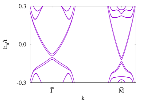
Figure 10: The band structure around $\bar{\Gamma}$ and $\bar{M}$ with magnetic moment $|J{\bf S}|=0.05$. A small potential gradient has been introduced to lift the surface degeneracy.

Fig. 11 shows our computed Berry’s curvature for the top surface state around $\bar{\Gamma}$ point for $|J{\bf S}|=0.10$ and $0.02$. It is evident that the most of the curvature accumulates around the symmetry point, which becomes more localized with decreasing magnetization strength $|J{\bf S}|$. We then calculate the Chern number by numerically integrating the curvature within a circle outside of which the curvature is very small, as indicated in Fig. 11. The “leakage” of Berry’s curvature outside this circle becomes increasingly negligible as $|J{\bf S}|$ becomes small, and we find that as $|J{\bf S}|\rightarrow 0$, the Chern number tends to $1/2$ as shown in Fig. 13. Similar behavior occurs around the $\bar{M}$ points. The Berry’s curvature illustrated in Fig. 12 clearly becomes more localized with decreasing magnetization, and the extrapolated integrated Berry’s curvature tends to $-1/2$, as shown in Fig. 13. Note that for the opposite surface, for magnetizations pointing outward at both surfaces, the Chern numbers for the Dirac spectra at the same type of symmetry point have opposite sign. This can be understood as a consequence of a combination of time-reversal and inversion symmetries (in the absence of the imposed potential gradient), which map states on each surface onto one another.

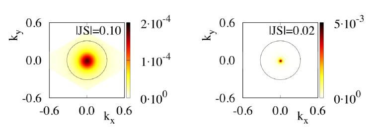
Figure 11: The Berry’s curvature for top surface state around $\bar{\Gamma}$ point with the magnetic moment $|J{\bf S}|$ as indicated.

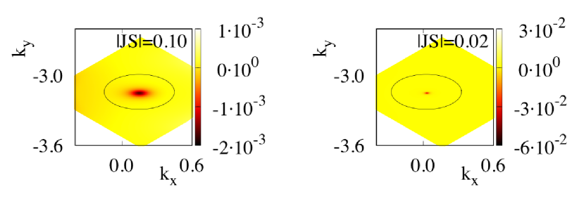
Figure 12: The Berry’s curvature for top surface state around $\bar{M}$ point with the magnetic moment $|J{\bf S}|$ as indicated.

These results have important consequences for DW’s, which connect regions with different uniform magnetizations. The change in Chern number topologically necessitates the presence of chiral, conducting bound states within a DW, with chirality given by the sign of that change Hatsugai (1993). For example, in the Ising case, where a DW connects states of magnetization parallel and antiparallel to the surface, one expects 1 and 3 states, of opposite chirality, for the $\bar{\Gamma}$ and $\bar{M}$ points, respectively. We now turn to numerical investigations that show this to be the case, and that it holds robustly with respect to parameters that characterize the details of the DW structure, as to be expected for a topologically protected property.

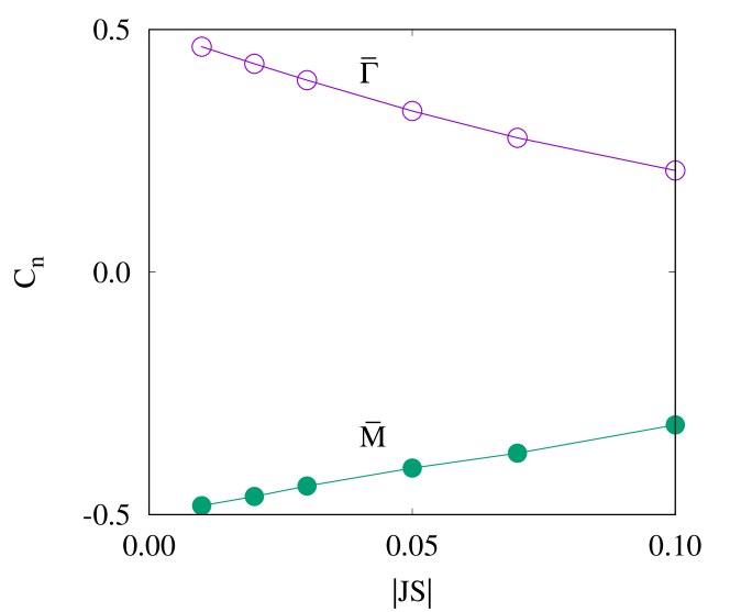
Figure 13: The extrapolation of Chern number with magnetic moment $|J{\bf S}|$ for top surface state. The bottom surface state has opposite behavior i.e., the values are opposite in sign.

IV.3 Domain Walls on a TCI Surface

We now turn to microscopic calculations of the electronic surface structure in the presence of a magnetization domain wall for our model TCI. Our goal is to explicitly demonstrate the presence of gapless, chiral conducting states within the surface energy gap generated by a uniform magnetization, as found in the previous section. We will see that the number for each chirality agrees with our expectations based on the Chern number calculations, and see that these are robust for different microscopic realizations of the DW magnetization profiles. The numerical approach will also allow us to assess the energy of a DW excitation, which is of particular interest in the context of situations where the ground state magnetization is along a $\Gamma$-$L_{i}$ direction, with $i=1,2,$ or 3. These directions are associated with the $\bar{M}$ points in the surface BZ, and there are six degenerate groundstate directions when the chemical potential is adjusted near the energy of the Dirac points associated with these locations Reja et al. (2017). These directions however come in two groups of 3, with components of the magnetization perpendicular to the surface either directed upward or downward. A priori it is unclear whether DW’s connecting states with the same perpendicular component or opposite ones is lower in energy; in our model we will see that the latter is lower in energy. This means that the system in these circumstances should be regarded as a six state system, rather than one with two sets of three states with a relatively large barrier separating states in different groups.

We begin by explaining how the numerical calculations are carried out.

IV.3.1 Projected Hamiltonian in Presence of Domain Wall

Our basic approach is to create a Hamiltonian with magnetization on the surfaces varying with position, to form a DW configuration. This means we will be working with very large unit cells, so that computation of the electron states becomes impractical for the full set of states in the slab geometry. We thus continue to exploit the technique of projecting the Hamiltonian into the low energy space of surface states. For simplicity we consider DW’s which run along the two highest symmetry directions on the surface, along the $k_{1}$ and $k_{2}$ directions illustrated in Fig. 9(c). Our supercells are very large along the cross-sectional direction of the DW, but as the magnetization is a function of displacement in only one direction, they can be very small in the direction perpendicular to this. Because the real space atoms on the surface are laid out in a triangular lattice, neighboring atoms in general will have displacements both parallel and perpendicular to the DW cross-section. To deal with this we allow our supercells to have a width containing two atoms along the narrow direction [see Fig. 9(b)], so that the magnetization need depend only on the position of an atom along the cross-sectional direction.

Thus, the supercell will be constructed of a line of small unit cells, defined by the primitive lattice vectors $a_{1}$ and $a_{2}$ shown in Fig. 9(b). The BZ associated with this doubled unit cell can be represented by a rectangle, as shown in (c) of the same figure. Notice this is half the size of a unit cell containing only one surface atom, so that $\bar{M}$ points of the latter falling outside of the former get folded in. In particular this means the $\bar{M}_{1}$ point will coincide in the smaller BZ with the $\bar{\Gamma}$ point, and the $\bar{M}_{2}$ and $\bar{M}_{3}$ points will coincide with one another.

We next need to generate a set of basis states that can represent a magnetization profile that varies slowly over many 2-atom unit cells. As a concrete example, suppose that the magnetization rotates as we move along the $a_{1}$ direction. If we impose periodic boundary conditions, we are required to have two DW’s separating regions of uniform magnetization in different directions. Let $N_{c}$ be the number of unit cells within which the full profile is contained. Our basis is generated for this large supercell in the absence any magnetic moments, by fixing $k_{2}$, and diagonalizing the Hamiltonian for a unit cell of the slab with only 2 surface sites, and with quantized values of $k_{1}$ of the form $k_{1}=k_{m}=2\pi m/N_{c};m=0,1,2,...(N_{c}-1)$. For each momentum, we retain only $N_{s}$ states with energies closest to the bulk gap, which capture the surface states. (Typically $N_{s}=8$ works well in our calculations.) We thus retain $N_{c}$x$N_{s}$ states in total for each of the quantized $k_{1}$ momenta. These basis states may be represented as

$$|k_{m},j\rangle \equiv \sum_{i}\alpha_{k_{m}}^{j}(i)|\alpha_{i}\rangle$$ (34)

$$= \frac{1}{\sqrt{N_{c}}}\sum_{n}e^{-ik_{m}x_{n}}|n,j\rangle\$$

where $|\alpha_{i}\rangle\equiv|i_{s},o_{i},s_{i}\rangle$ represents basis states indexed by site $i_{s}=1,2,...2$x$47$, $o_{i}=(p_{x},p_{y},p_{x})$ the orbital index, and $s_{i}=(\uparrow,\downarrow)$ the local spin index. The quantities $x_{n}$ denote the positions of the two atom unit cells within the larger supercell. Thus for each $k_{m}$, we have retained $j=1,2,...N_{s}$ states, which we will use for the basis of our Hilbert space. The energy eigenvalue (again, in the absence of any magnetization) for the state $|k_{m},j\rangle$ is denoted by $E_{k_{m},j}$.

Rewriting our basis in real space by inverting the Fourier transform,

$$|n,j\rangle=\frac{1}{\sqrt{N_{c}}}\sum_{k_{m},j}e^{ik_{m}x_{n}}|k_{m},j\rangle,\$$ (35)

we can now introduce surface magnetic moments into the Hamiltonian, writing as $H_{n}$ the projection of the $sd$ Hamiltonian for the two sites in the cell located at $x_{n}$, with each site containing the values of ${\bf S}_{i}$ determined by the presumed magnetization profile of the DW. With this addition, the effective Hamiltonian matrix for our system becomes

$$\langle k_{m},j|H_{eff}|k_{m^{\prime}},j^{\prime}\rangle=\frac{1}{N_{c}}\sum_{n=0}^{N_{c}-1}\langle k_{m},j|H_{n}|k_{m^{\prime}},j^{\prime}\rangle e^{i{(k_{m}-k_{m^{\prime}})}x_{n}}+E_{k_{m},j}\delta_{k_{m},k_{m^{\prime}}}\delta_{j,j^{\prime}}.$$ (36)

Note again that this matrix is dependent implicitly on the value of $k_{2}$, the wavevector in the direction along which the DW runs. This matrix is considerably reduced in size from what one has for the tight-binding model of the full slab with a magnetization profile on its surface, and allows us to compute energy states of the electrons as a function of $k_{2}$. For DW’s running along the $a_{1}$ direction, we construct an effective Hamiltonian in a very analogous way.

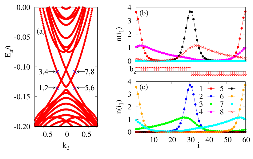
Figure 14: (a) Energy bands $E_{n}$ near $\bar{\Gamma}$ when a Neel domain wall of width $d=0$ runs along $k_{2}$. The electron density $n(i_{1})$ for the representative DW states (indicated by blue cross points and numbered $1,2...$) along the unit cell direction $a_{1}$ are shown in (b) and (c) for top and bottom surfaces respectively of the slab with (111) surfaces. The component of magnetic moments $b_{z}$ along $\Gamma-{L}_{0}$ direction are shown by red arrows between panels (b) and (c) .

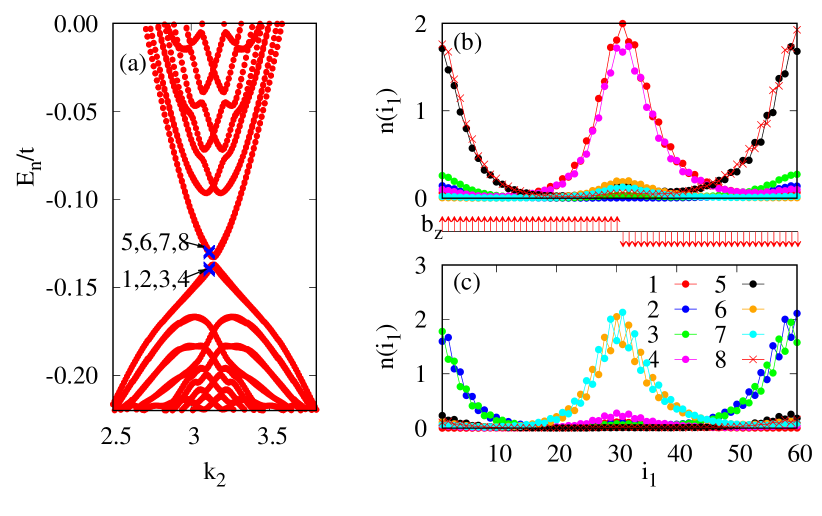
Figure 15: Energy bands $E_{n}$ [panel (a)] and electron densities [panels (b), (c)] of bound DW states near the $\bar{Y}$ point for the DW configuration as described in Fig. 14.

IV.3.2 Results

With this formalism, we now compute electronic structures for different DW configurations. We expect to find states invading the gaps present in the surface electronic structure when there is a uniform magnetization. These occur near two places (see Fig. 9). (i) The center of the rectangular BZ where $\bar{\Gamma}$ and $\bar{M}_{1}$ overlap due to zone-folding. (ii) The projection of the $\bar{M}_{2}$ and $\bar{M}_{3}$ points onto the $k$-axis running along the DW. The latter corresponds to either the $\bar{X}$ or the $\bar{Y}$ point in the reduced Brillouin zone shown in Fig. 9(c), depending on which direction the DW runs along. We will see that the in-gap states appear when the projection of the magnetic moments along any of the bulk $\Gamma$-$L$ directions changes sign inside the DW cross-section. We expect from our Chern number analysis that the number of in-gap branches depends on the number of such projections changing sign.

We first consider the case of DWs connecting different states with magnetic moments along the $\Gamma$-$L_{0}$ axis, with the DW’s running along the $a_{2}$ direction. [See Fig. 9(b)]. In this case the magnetic moments rotate as we move in the $a_{1}$ direction within a DW, and the rotation is in the plane defined by the direction perpendicular to the surface and the $a_{1}$ direction. This represents a Néel domain wall Chaikin and Lubensky (1995). The geometry of our supercell includes two regions of width $N_{s}-2d$ with uniform magnetization, one pointing “up” and the other “down”, connected by two DW’s of width $d$ within which the magnetization rotates uniformly. We consider several values of $d$, including $d=0$ for which the change in magnetization is abrupt.

Fig. 14(a) illustrates the band structure near the $\bar{\Gamma}$ point as a function of $k_{2}$ for a DW with $d=0$ and $|J{\bf S}|=0.1$. As noted above, the $\bar{\Gamma}$ point hosts two Dirac points, associated with the surface projections of the bulk $L_{0}$ and $L_{1}$ points, due to zone-folding of the original hexagonal Brillouin zone [Fig. 9(c)]. Since this DW configuration induces a sign change in the component of magnetic moments along the $\Gamma-{L}_{0}$ and the $\Gamma-{L}_{1}$ directions, we expect to find two chiral states associated with these. Because we have two surfaces, each with two DW’s, this leads to an expectation of 8 chiral states. Fig. 14(a) shows this is indeed true. (Note each of the states in the figure is exactly doubly degenerate, due to a combination of time-reversal and inversion symmetries.) Figs. 14(b) and (c) show the electron densities of representative states from the different chiral branches, for each of the DW’s on the top and bottom surface. It is clear that each of the DW’s hosts two chiral states, running in opposite directions. This is consistent with the Chern number change we found in the last section, which was $\pm 1$ for the $\bar{\Gamma}$ point, and $\mp 1$ for a $\bar{M}$ point. Note the small gap opening at $k_{2}=0$ near energy -0.14 occurs due to admixture of DW states associated with the $\bar{M}$ point on the same surface: as the densities in Figs. 14(b,c) show, the localization lengths for these states are still relatively large compared to our inter-DW separation, even for the large unit cells we use. This is a reflection of the fact that within the uniformly magnetized regions, the magnetization is not parallel to the $\Gamma-{L}_{1}$ direction, so the gaps induced in the Dirac points at $\bar{M}$ are relatively small.

In contrast, the band structure near $\bar{Y}$ associated with this magnetization profile yields states in each DW with the same chirality. This is shown in Fig.15. For example, the states labeled 1 and 4 disperse in the same direction, and are located in the same DW. Analogous calculations (not shown) of DW’s running perpendicular to the structure relevant for Figs. 14 and 15 yield analogous results. We thus confirm that the net chirality of DW states connecting groundstates with magnetizations along the $\Gamma-{L}_{0}$ axis, but in opposite directions, have net chirality of 2. This is just as expected from our Chern number analysis.

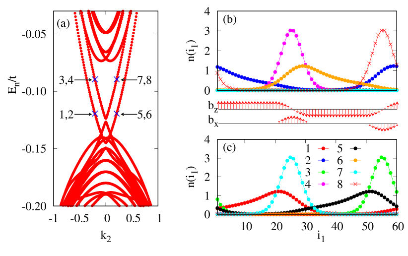
Figure 16: (a) Energy bands $E_{n}$ near $\bar{\Gamma}$ when a Neel domain wall of width $d=10$ runs along $k_{2}$. The electron density $n(i_{1})$ for DW states (indicated by blue cross points and numbered $1,2...$) along the unit cell direction $a_{1}$ are shown in (b) and (c) for top and bottom surfaces respectively of the slab with (111) surfaces. The component of magnetic moments $b_{z}$ along $\Gamma-{L}_{0}$ and $b_{x}$ along $a_{1}$ directions are shown by red arrows between panels (b) and (c).

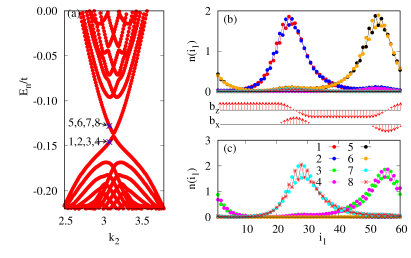
Figure 17: Energy bands $E_{n}$ [panel (a)] and electron densities [panels (b), (c)] of bound DW states near the $\bar{Y}$ point for the DW configuration as described in Fig.16.

Further analogous calculations may be carried through for other geometries. For example, Figs. 16 and 17 illustrate results for wider DW’s, $d=10$. The results are qualitatively very similar to our $d=0$ results, importantly showing the same types of chiral states near the $\bar{\Gamma}$ and $\bar{Y}$ points as for $d=0$, and the same net chirality for the DW’s that we expect based on the Chern number analysis. We have found other values of $d$, both larger and smaller, yield these types of results as well. In addition we have performed calculations for Bloch walls – profiles in which the rotation axis of the magnetization inside the DW is parallel rather than perpendicular to the direction along which the DW runs – and again find the same basic results. As might be expected for topologically determined properties, the chirality of DW’s in this system seems rather robust.

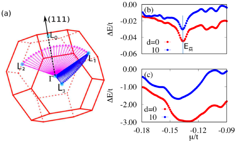
Figure 18: (a) DW configurations connecting (i) $\Gamma-L_{1}$ to $\Gamma-L_{2}$ directions (magenta), (ii) $\Gamma-L_{1}$ to $\Gamma-L_{3}$ directions (blue). (b) The energy difference between these configurations $\Delta E=E_{ii}-E_{i}$ as a function of chemical potential $\mu$ for $d=0,10$ and $|J{\bf S}|=0.01$ showing minimum when $\mu$ is close to $\bar{M}$ Dirac point energy $E_{\bar{M}}$. (c) $\Delta E$ for larger $|J{\bf S}|=0.10$

We also wish to consider DW’s connecting different states associated with magnetization groundstates along the $\Gamma-L_{1,2,3}$. These are energetically stable when the chemical potential is near the energy of the Dirac points associated with $\bar{M}$ points. As mentioned above, what is not a-priori obvious is whether DW’s that connect groundstates with the same sign of of magnetization along the direction perpendicular to the surface will be higher or lower in energy than those connecting neighboring magnetization states with opposite such projections. Our calculations support that it is in fact the second of these that is energetically favorable. To show this, we consider DW configurations as shown in Fig. 18(a). There are two cases: (1) one which connects the $\Gamma-{L}_{1}$ to $\Gamma-{L}_{2}$ directions (magenta), and (ii) one which connects the $\Gamma-{L}_{1}$ direction to the $\Gamma-{L}_{3}$ direction (blue). Using the technique described above, we compute the single-particle energy states for each of the two structures, and then add all the energies below the Fermi energy $\mu$ to obtain a total energy associated with the magnetization profile. The energy difference of these, $\Delta E=E_{ii}-E_{i}$, as a function of $\mu$, is shown in Fig.18 (b) for $|J{\bf S}|=0.01$ and $d=0,10$ as indicated. We find that the DW configuration (ii) is favorable over (i), and moreover that $\Delta E$ has a local minimum, when $\mu$ is close to the $\bar{M}$ Dirac point energy, $E_{\bar{M}}$. This has the important consequence of making all six groundstate configurations equally accessible from some given starting state, yielding a six state clock model. If $\mu$ is near $E_{\bar{M}}$ we expect, as discussed above, that system will thermally disorder at sufficiently high temperature via a Kosterlitz-Thouless transition José et al. (1977).

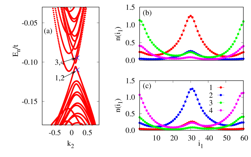
Figure 19: (a) Energy bands $E_{n}$ at $\bar{\Gamma}$ for DW configuration corresponding to ($ii$) in Fig. 18(a), with $d=0$. The density of electron $n(i_{1})$ for the representative DW states (indicated by blue cross points and numbered $1,2...$) along the unit cell direction $a_{1}$ are shown in (b) and (c) for top and bottom surfaces respectively of the slab with (111) surfaces.

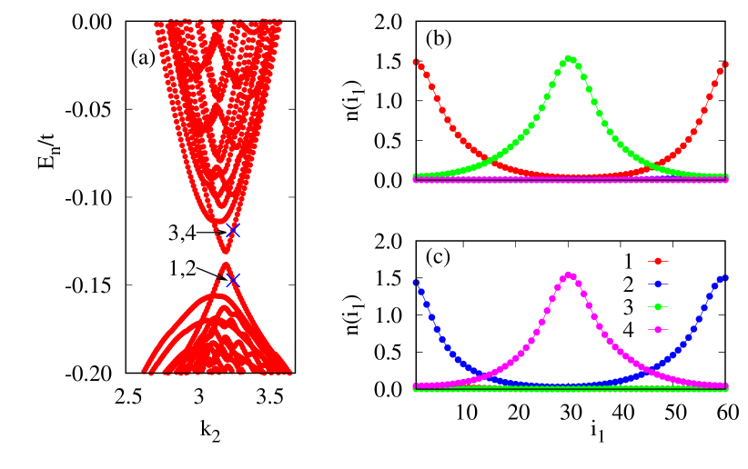
Figure 20: (a) Energy bands $E_{n}$ near $\bar{Y}$ for DW configuration corresponding to ($ii$) in Fig. 18(a), with $d=0$, for momentum along $k_{2}$. The electron density $n(i_{1})$ for the representative DW states (indicated by blue cross points and numbered $1,2...$) along the unit cell direction $a_{1}$ are shown in (b) and (c) for top and bottom surfaces respectively of the slab with (111) surfaces.

Finally, it is interesting to contrast the nature of the in-gap states hosted by these DW’s with those relevant to magnetizations along the $\Gamma-{L}_{0}$ axis. Examination of Fig. 18(a) reveals that while the magnetization projection along the $\Gamma-{L}_{1}$ and $\Gamma-{L}_{3}$ directions does not change sign, those along the $\Gamma-{L}_{0}$ and $\Gamma-{L}_{2}$ directions do. This means for a DW running along the $k_{2}$ direction, we should find a single chiral state near each of the $\bar{\Gamma}$ and $\bar{Y}$ points. Figs. 19 and 20 demonstrate that this indeed happens. Note that the chiral directions of the two modes are oppositely oriented within a given DW, so that the net chirality vanishes. This is consistent with our observation, in the previous section, that the $\bar{M}$ and $\bar{\Gamma}$ Chern numbers have opposite signs. This can have interesting consequences for differing electrical behaviors due to DW’s when $\mu$ is near the energy of the Dirac points at $\bar{M}$ as opposed to that of the $\bar{\Gamma}$ point. We discuss this further in the next and final section of this paper.

V Summary, Discussion, and Future Directions

In this paper we studied domain walls of ferromagnetic systems, in which the magnetic degrees of freedom mutually interact through their impact on Dirac electrons on a surface. Such models arise naturally in the context of topological insulators protected by time-reversal symmetry (TI’s) and topological crystalline insulators (TCI’s), and are very commonly studied perturbatively, using varieties of the RKKY analysis. In our study we demonstrated that if magnetic order does set in this type of system, the energetics of magnetization gradients may become anomalous, in a way that is in principle controllable. When the surface electron density is such that there is a Fermi surface, the interactions effectively cut off at a length scale of order $1/k_{F}$, above which there are $2k_{F}$ oscillations in the RKKY coupling. As $k_{F}\rightarrow 0$, the coupling retains its sign, and the RKKY analysis predicts a (well-known) $1/R^{3}$ fall-off in the coupling. In a coarse-grained description of the system, this means that the appropriate gradient term for the magnetization at low temperature becomes anomalous, acquiring an emergent long-range form, with true long-range interactions among magnetization gradients being the limiting behavior as the magnetization magnitude vanishes. For non-vanishing scale of magnetization, the gradient energy can be properly described by a form that is quadratic in wavevector, but acquires a non-analytic form in the magnetization itself.

The emergent long-range form of the interaction impacts, among other things, interactions among DW’s, since these involve a fixed change in magnetization. From our analysis of the gradient energies, we showed that the emergent interaction induces logarithmic interactions between DW’s, up to a length scale set by the magnetization itself. Using an effective Dirac model in conjunction with a transfer matrix method, we were able to verify the presence of this interaction, and found moreover that it results from a subtle cancellation in the energies associated with bound states in the DW’s and phase shifts of unbound electrons scattering from them. A tight-binding system involving graphene with a position-dependent mass term that models DW pairs corroborated the result.

We then considered DW’s in a more concrete system, a model of (Sn/Pb)Te alloys that are a paradigm for TCI systems. We considered the (111) surface, which hosts particularly rich physics in this context, because it hosts Dirac points at two different, distinct energies, a single isolated Dirac point (near the surface $\bar{\Gamma}$ point) and, at slightly lower energy, a group of three degenerate Dirac points (near three $\bar{M}$ points), allowing for different types of DW’s. We carried out a numerical Berry’s phase analysis on the electronic states around these points in the presence of a uniform magnetization, and demonstrated that they carry Chern numbers of opposite sign, $\pm 1/2$. When the chemical potential is adjusted such that the $\bar{\Gamma}$ point dominates the energetics of the magnetization, the resulting DW excitations are predicted to induce a change of Chern number given by $\pm 2$. This suggests the DW’s host in-gap states with a net chirality. We demonstrated that this is true using a numerical low-energy projection scheme for the tight-binding slab, and showed that it arises as a net effect of four in-gap states, with two running in opposite directions, and another pair running in the same direction. For cases where the $\bar{M}$ Dirac points dominate the magnetization energy, we found that the lowest energy DW’s of equally connect six possible groundstate orientations, and in this case yield two conducting states of opposite chirality.

The conducting states of DW’s in these systems are of considerable interest, because they allow their presence to be detected electrically. DW’s can be forced into the system, for example, by cooling it from high temperature in zero field. The DW’s can be detected in principle by a variety of techniques, by looking for their contribution to the conductance of the surface. This could be investigated by transport studies, tunneling measurements, or even surface reflectance. The behavior of the system as the chemical potential is changed should reveal the different regimes of the low-energy DW’s, as the system is tuned through different behaviors of the gradient energy, as well as through Fermi energy scales where different Dirac points may dominate the magnetization dynamics. It is interesting to note, for example, that in the two-fold case (one low-energy magnetization axis) the DW’s should be strongly conducting due to their chirality, whereas in the six-fold case, the vanishing chirality will allow backscattering between the in-gap states in a DW, leading to a smaller contribution to the surface conductance. Beyond this, an estimation of the critical temperature $T_{c}$, based on balancing of energy and entropy of a DW, reveals a crossover from a $T_{c}\sim n_{imp}^{2}$ when the Fermi surfaces are closed loops to $T_{c}\sim n_{imp}$ when there is a point-like Fermi surface (i.e., when the Fermi energy passes through a Dirac point.) This behavior is illustrated in Fig. 21.

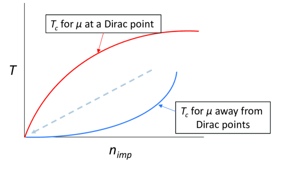
Figure 21: Schematic phase diagram for classical magnetic impurities coupled by surface Dirac electrons, contrasting behavior of the critical temperature $T_{c}$ vs. impurity density $n_{imp}$ when the Fermi energy $\mu$ passes through a Dirac point (red) with when it does not (blue). Dashed illustrates illustrates a trajectory in which the in-gap states associated with domain walls will produce pseudogap behavior in the electronic spectrum, and where the interactions among the DW’s become increasingly long range moving down the trajectory, enhancing the density of states within the mean-field gap.

While our detailed analyses of these systems have largely focused on the low-energy behavior of the topological DW excitations, it is interesting to consider the consequences of our results for higher temperatures. In particular, approaching a phase boundary for some magnetic impurity density $n_{imp}$, $T_{c}(n_{imp})$, one expects the average magnetization to become vanishing small as DW’s come increasingly close to proliferating. However, this does not imply that the interactions among the DW’s become unlimited in range: in such a situation, the stiffness becomes limited by $k_{B}T$, rather than the magnetization scale not (b). For example, a calculation akin to that of Sec. II.2.2 at finite temperature $T$ reveals that the energy cost to introduce an magnetization gradient $g$ in graphene behaves as $\Delta E(g)\sim g^{2}b_{0}^{2}/T$ unp . This indicates that the long-range behavior of the stiffness will be cut off by finite temperature if the magnetization scale is small. Thus, true long-range interactions in this system emerge if one approaches the low-temperature, low impurity density point, as illustrated in by the dashed arrow in Fig. 21. In approaching this point, interactions among DW’s of unlimited range emerge. It is interesting to note that the in-gap states hosted by finite size DW’s will in principle fill the mean-field gap in the Dirac electron spectrum, but the density of states associated with these will drop rapidly approaching zero energy as DW’s of increasing size (which will host the lowest energy in-gap states) are exponentially unlikely to be found in the system when in the ordered state. The emergent long-range interactions will enhance the average area occupied by DW’s and their associated induced states in the gap relative to systems with short-range gradient interactions. In principle, this behavior should be directly accessible in tunneling experiment.

The studies we have reported in this paper suggest many other directions for future exploration. Important among these is that, in our approach to these systems, we have treated the magnetic moments as classical. Clearly at sufficiently low temperature a quantum treatment would be more appropriate. For example, we have ignored the possibility of non-trivial correlations between conduction electron spins and the impurity spins that occur in the Kondo effect, although this physics should set in at extremely low temperature when the $sd$ coupling scale $J$ is small Allerdt et al. (2017). Beyond this, it is interesting to note the connection of this system with “chiral magnets,” not (c) magnetic systems coupled to chiral fermions Rosenstein et al. (1993); Knorr (2016); Otsuka et al. (2016); Li et al. (2017); He et al. (2018); Yin et al. (2018), which are known to support quantum phase transitions with their own unique critical behaviors. Note that while such systems are similar to the ones we focus upon, these are generally formulated as magnets supporting their own independent gradient interactions, exchange-coupled to chiral fermions, while in the systems we are considering, interactions among the magnetic moments arise solely from exchange coupling with the Dirac electrons. From the perspective of an renormalization group (RG) analysis the systems may be connected, in which case the origin in Fig. 21 will move to a non-vanishing value of $n_{imp}$. The classical behavior discussed in our work will nevertheless present itself as crossover behavior prior to quantum critical behavior sufficiently close to the transition point. Our studies demonstrate that interesting fluctuation behavior appears in this system even away from the quantum critical regime.

Related to this, systems such as graphene, in which spin-orbit coupling is largely irrelevant so that the magnetization enjoys continuous symmetries, offer further possibilities for study. Interacting electrons in graphene without external magnetic moments can be formally recast in terms of non-interacting electrons with an auxiliary Hubbard-Stratanovich field Knorr (2016), suggesting a quantum phase transition in the universality class of the Gross-Neveu model Herbut (2006). How this picture changes when real quantum spins couple to the electrons remains an interesting area to investigate. While the continuous symmetry of the order parameter implies that thermal fluctuations at any non-zero temperature disorder the system Mermin and Wagner (1966), the non-analytic behavior of the system with respect to spin gradients at short wavelengths suggest that interesting collective modes can be present in this regime. Moreover, the effect of thermal disordered magnetic moments on the electron states of this system should have interesting consequences for thermal and transport properties of the system.

Finally, effects of disorder have been assumed throughout this paper to sufficiently average that its effects may be ignored at a qualitative level. This seems most likely for situations where the effective interactions have become sufficiently long range, but when the interaction length scale is fixed by a Fermi momentum, they are likely to become more important. In addition, electron-electron interactions have been ignored throughout our study. In systems where Fermi surfaces and Dirac points may coexist at the same energy – such as the (111) TCI surface – these will be screened and are likely to be qualitatively unimportant. Other surfaces, such as TI systems or the (100) surface of the (Pb/Sn)Te TCI system, can become fully gapped, and here we expect logarithmic, repulsive interactions among DW’s because of the charge they contain. These interactions will be present to arbitrarily large distance even at finite $T$, and whether they impact classical thermal phase transitions in these systems is another interesting direction to explore.

Clearly, magnetic degrees of freedom coupled by Dirac electrons host a rich variety of physical phenomena. Under many circumstances, these systems support domain walls as fundamental topological excitations, which reflect the interesting effective interactions induced among the magnetic moments, as well as the topological nature of the electronic system that couples them. Their behavior, both thermal and electrical, offer exciting windows into the special properties of electrons in such topologically non-trivial systems.

Acknowledgements – The authors gratefully acknowledge useful discussions with Ganpathy Murthy, R. Shankar, Efrat Shimshoni, Kai Sun, and Shixiong Zhang. This work was supported by the NSF through Grant Nos. DMR-1506263 and DMR-1506460, by the US-Israel Binational Science Foundation, and by MEyC-Spain under grant FIS2015-64654-P. HAF thanks the Aspen Center for Physics, where part of this work was done. Computations were carried out on the ITF/IFW and IU Karst clusters.

VI Appendix

In this Appendix we provide a few details of the stiffness calculations whose results are described in Section II. We begin first with the case where the Fermi energy is in the gap, from Eq. 5, which we reproduce for convenience:

$$\Delta E=-{1\over 4}\sum_{\bf q}\left\{\frac{|\langle{\bf q},-|\delta{\bf b}\cdot\vec{\sigma}|{\bf q}-{\bf Q},+\rangle|^{2}}{\varepsilon_{0}({\bf q})+\varepsilon_{0}({\bf q}-{\bf Q})}+\frac{|\langle{\bf q},-|\delta{\bf b}\cdot\vec{\sigma}|{\bf q}+{\bf Q},+\rangle|^{2}}{\varepsilon_{0}({\bf q})+\varepsilon_{0}({\bf q}+{\bf Q})}\right\}.$$ (37)

To find the gradient energy we expand this to quadratic order in $Q$. A long but in principle straightforward calculation brings us to the expression

$$\Delta E({\bf Q})-\Delta E(0)\approx{1\over{32}}\sum_{\mu,\nu=x,y}Q_{\mu}Q_{\nu}\sum_{\bf q}\Biggl{\{}\frac{|\langle{\bf q},-|\delta{\bf b}\cdot\vec{\sigma}|{\bf q},+\rangle|^{2}}{\varepsilon_{0}({\bf q})^{2}}\partial_{\mu}\partial_{\nu}\varepsilon_{0}({\bf q})$$

$$-{1\over{\varepsilon_{0}({\bf q})}}\partial_{\mu}\partial_{\nu}|\langle{\bf q},-|\delta{\bf b}\cdot\vec{\sigma}|{\bf q},+\rangle|^{2}\Biggr{\}}$$ (38)

This expression is explicitly quadratic in $Q$ and $\delta b$. As discussed in the main text it is natural to introduce a tensor $g_{\mu\nu}^{ij}$ characterizing the energy cost, so that $\Delta E({\bf Q})-\Delta E(0)={{\Omega}\over{2}}\sum_{\mu,\nu=x,y}\sum_{ij=x,y,z}g_{\mu\nu}^{ij}Q_{\mu}Q_{\nu}\delta b_{i}\delta b_{j}$. The $g$ coefficients can read off from Eq. 38, and for fixed $\delta\bf{b}$ one can use them to assess the energy cost for introducing a slow gradient in the magnetization. More explicit expressions for the $g$’s require a matrix element, which can found using Eq. 3. This yields

$$|\langle{\bf q},-|\delta{\bf b}\cdot\vec{\sigma}|{\bf q},+\rangle|^{2}=\left\{\left[q^{2}\delta b_{z}-b_{z}{\bf q}\cdot\delta{\bf b}\right]^{2}+\varepsilon_{0}(q)^{2}\left[\hat{z}\cdot({\bf q}\times\delta{\bf b})\right]^{2}\right\}/[q\varepsilon_{0}(q)]^{2},$$ (39)

which in turn provides integral expressions of the form

$$\sum_{ij}g_{\mu\nu}^{ij}\delta b_{i}\delta b_{j} = {{1}\over{\Omega}}\sum_{\bf q}\frac{2\delta_{\mu\nu}-4q_{\mu}q_{\nu}/\varepsilon_{0}(q)^{2}}{q^{2}\varepsilon_{0}(q)^{5}}$$ (40)

$$\times \left\{q^{4}\delta b_{z}^{2}+b_{z}^{2}\left(q_{x}^{2}\delta b_{x}^{2}+q_{y}^{2}\delta b_{y}^{2}\right)+\varepsilon_{0}(q)^{2}\left(q_{x}^{2}\delta b_{y}^{2}+q_{y}^{2}\delta b_{x}^{2}\right)-2q^{2}q_{x}q_{y}\delta b_{x}\delta b_{y}\right\}.$$

It is immediately apparent that only $g_{\mu\nu}^{zz}$ and $g_{\mu\nu}^{ij}$ with $i,j=x,y$ are non-vanishing, so that gradients in $\delta b_{z}$ can be assessed separately from gradients in $\delta b_{x,y}$. The various non-vanishing values of $g_{\mu\nu}^{ij}$ can now be read off in integral forms, all of which are analytically tractable. The explicit results are given in Eqs. 6 and 7.

We next consider the case when the Fermi energy passes through a band. Our starting point is now the expressions for $\Delta E_{+}$ and $\Delta E_{-}$. The former is given by Eq. 9, which again we reproduce for convenience:

$$\Delta E_{+}={1\over 4}\sum_{\mathclap{\begin{subarray}{c}q>k_{F}\\ |{\bf q}-{\bf Q}|<k_{F}\end{subarray}}}\frac{|\langle{\bf q},-|\delta{\bf b}\cdot\vec{\sigma}|{\bf q}+{\bf Q},-\rangle|^{2}}{\varepsilon_{0}({\bf q}+{\bf Q})-\varepsilon_{0}({\bf q})}-{1\over 4}\sum_{q>k_{F}}\frac{|\langle{\bf q},-|\delta{\bf b}\cdot\vec{\sigma}|{\bf q}+{\bf Q},+\rangle|^{2}}{\varepsilon_{0}({\bf q}+{\bf Q})+\varepsilon_{0}({\bf q})},$$ (41)

and again $\Delta E_{-}$ has the same form as Eq. 9, with ${\bf Q}\rightarrow-{\bf Q}$. The constraints on the wavevector sums can be simplified by defining a step function,

$$f_{\bf q}=\Biggl{\{}\begin{array}[]{c c}0&\quad q<k_{F},\\ 1&\quad q>k_{F},\end{array}$$ (42)

and a unit vector $\hat{h}_{\bf q}\equiv(q_{x},q_{y},b_{z})/\varepsilon_{0}(q)$. Using Eq. 3 to compute the matrix elements, with considerable algebra one can reformulate $\Delta E$ as $\Delta E\equiv\Delta E_{+}^{(1)}+\Delta E_{+}^{(2)}+\Delta E_{-}^{(1)}+\Delta E_{-}^{(2)}$ where

$$\Delta E_{-}^{(1)} = {1\over 4}\sum_{\bf q}f_{\bf q}\frac{|\delta{\bf b}|^{2}\left[\varepsilon_{0}(q)-\hat{h}_{-{\bf q}-{\bf Q}}\cdot\hat{h}_{-{\bf q}}\varepsilon_{0}(|{\bf q}-{\bf Q}|)\right]}{\varepsilon_{0}^{2}(|{\bf q}+{\bf Q}|)-\varepsilon_{0}^{2}(q)},$$ (43)

$$\Delta E_{-}^{(2)} = {1\over 2}\sum_{\bf q}f_{\bf q}\frac{\left[(\delta{\bf b}\cdot\hat{h}_{-{\bf q}-{\bf Q}})(\delta{\bf b}\cdot\hat{h}_{-\bf q})\right]\varepsilon_{0}(|{\bf q}+{\bf Q}|)}{\varepsilon_{0}^{2}(|{\bf q}+{\bf Q}|)-\varepsilon_{0}^{2}(q)},$$ (44)

and $\Delta E_{+}^{(i)}$ of the same form as $\Delta E_{-}^{(i)}$, but with ${\bf Q}\rightarrow-{\bf Q}$, up to terms that cancel when the $\Delta E_{\pm}^{(i)}$’s are summed together to form $\Delta E$.

We now proceed to show $\Delta E^{(1,2)}_{\pm}$ are actually independent of ${\bf Q}$. Defining $\phi$ as the angle between Q and q, and introducing an upper momentum cutoff $\Lambda$, one finds for large $\Omega$

$$\Delta E_{-}^{(1)} = -\frac{\Omega|\delta{\bf b}|^{2}}{16\pi^{2}}\int_{k_{F}}^{\Lambda}dq\frac{q^{2}}{Q\varepsilon_{0}(q)}\int_{0}^{2\pi}d\phi\frac{\cos\phi}{2\frac{q}{Q}\cos\phi+1}$$ (45)

$$= -\frac{\Omega|\delta{\bf b}|^{2}}{16\pi^{2}}\int_{k_{F}}^{\Lambda}dq\frac{q^{2}}{Q\varepsilon_{0}(q)}\left(\frac{\pi Q}{q}\right)$$

which is manifestly $Q$-independent. Clearly the same will be true of $\Delta E_{+}^{(1)}$. For the remaining contribution to $\Delta E$ is is helpful to combine $\Delta E_{+}^{(2)}$ and $\Delta E_{-}^{(2)}$, which can be cast in the form

$$\Delta E_{+}^{(2)} + \Delta E_{-}^{(2)}=-\sum_{\bf q}\frac{f_{\bf q}}{\varepsilon_{0}(q)}\left\{\frac{\delta{\bf b}\cdot({\bf q}+{\bf Q})\delta{\bf b}\cdot{\bf q}+\delta b_{z}^{2}b_{z}^{2}}{\varepsilon_{0}^{2}(|{\bf q}+{\bf Q}|)-\varepsilon_{0}^{2}(q)}\right\},$$ (46)

The term $\delta b_{z}^{2}$ in Eq. 46 vanishes upon integration over $\phi$. For the remaining two terms we write $\delta{\bf b}$ in the form

$$\delta{\bf b}=\delta b_{\parallel}\hat{Q}+\delta b_{\perp}\hat{z}\times\hat{Q}+\delta b_{z}\hat{z}.$$

In terms of these quantities, one finds

$$\Delta E_{+}^{(2)} + \Delta E_{-}^{(2)}=-\sum_{\bf q}\frac{f_{\bf q}}{\varepsilon_{0}(q)}\left\{\frac{\left[\delta b_{\parallel}^{2}-\delta b_{\perp}^{2}\right]q^{2}\cos^{2}\phi+Qq\delta b_{\parallel}^{2}\cos\phi}{\varepsilon_{0}^{2}(|{\bf q}+{\bf Q}|)-\varepsilon_{0}^{2}(q)}\right\}$$ (47)

$$= -\frac{\Omega}{4\pi^{2}Q^{2}}\int_{k_{F}}^{\Lambda}dq\frac{q}{\varepsilon_{0}(q)}\int_{0}^{2\pi}\frac{\left[\delta b_{\parallel}^{2}-\delta b_{\perp}^{2}\right]q^{2}\cos^{2}\phi+Qq\delta b_{\parallel}^{2}\cos\phi}{2\frac{q}{Q}\cos\phi+1}$$

$$= -\frac{\Omega}{4\pi^{2}Q^{2}}\int_{k_{F}}^{\Lambda}dq\frac{q}{\varepsilon_{0}(q)}\left\{q^{2}\left[\delta b_{\parallel}^{2}-\delta b_{\perp}^{2}\right]\left(-\frac{\pi Q^{2}}{2q^{2}}\right)+Qq\delta b_{\parallel}^{2}\left(\frac{\pi Q}{q}\right)\right\},$$

which is again manifestly independent of ${\bf Q}$. We thus see that, provided $Q<\mu$, the energy required to introduce an oscillation in the magnetization is independent of the oscillation wavevector. This indicates that an effective energy functional for the magnetization should have vanishing coefficient for the quadratic gradient term – effectively, a vanishing spin stiffness. This contrasts dramatically with the situation we found for $\mu=0$, where the stiffness diverged as $b_{z}\rightarrow 0$.

References

- Ruderman and Kittel (1954) M. A. Ruderman and C. Kittel, Phys. Rev. 96, 99 (1954), URL https://link.aps.org/doi/10.1103/PhysRev.96.99.
- Kasuya (1956) T. Kasuya, Progr. Theoret. Phys. 16, 45 (1956).
- Yosida (1957) K. Yosida, Phys. Rev. 106, 893 (1957), URL https://link.aps.org/doi/10.1103/PhysRev.106.893.
- C.Kittel (1968) C.Kittel, Sol. St. Phys.: Advances in Research and Applications 22, 1 (1968).
- Fischer and Klein (1975) B. Fischer and M. W. Klein, Phys. Rev. B 11, 2025 (1975), URL https://link.aps.org/doi/10.1103/PhysRevB.11.2025.
- Ketterson (2016) J. Ketterson, The Physics of Solids (Oxford University Press, 2016).
- Dugaev et al. (2006) V. K. Dugaev, V. I. Litvinov, and J. Barnas, Phys. Rev. B 74, 224438 (2006), URL https://link.aps.org/doi/10.1103/PhysRevB.74.224438.
- Brey et al. (2007) L. Brey, H. A. Fertig, and S. Das Sarma, Phys. Rev. Lett. 99, 116802 (2007), URL http://link.aps.org/doi/10.1103/PhysRevLett.99.116802.
- Saremi (2007) S. Saremi, Phys. Rev. B 76, 184430 (2007), URL https://link.aps.org/doi/10.1103/PhysRevB.76.184430.
- Black-Schaffer (2010) A. M. Black-Schaffer, Phys. Rev. B 81, 205416 (2010), URL https://link.aps.org/doi/10.1103/PhysRevB.81.205416.
- Fabritius et al. (2010) T. Fabritius, N. Laflorencie, and S. Wessel, Phys. Rev. B 82, 035402 (2010), URL https://link.aps.org/doi/10.1103/PhysRevB.82.035402.
- Sherafati and Satpathy (2011) M. Sherafati and S. Satpathy, Phys. Rev. B 84, 125416 (2011), URL https://link.aps.org/doi/10.1103/PhysRevB.84.125416.
- Kogan (2011) E. Kogan, Phys. Rev. B 84, 115119 (2011), URL https://link.aps.org/doi/10.1103/PhysRevB.84.115119.
- Lee et al. (2012) H. Lee, E. R. Mucciolo, G. Bouzerar, and S. Kettemann, Phys. Rev. B 86, 205427 (2012), URL https://link.aps.org/doi/10.1103/PhysRevB.86.205427.
- Roslyak et al. (2013) O. Roslyak, G. Gumbs, and D. Huang, Journal of Applied Physics 113, 123702 (2013), eprint https://doi.org/10.1063/1.4795624, URL https://doi.org/10.1063/1.4795624.
- Gorman et al. (2013) P. D. Gorman, J. M. Duffy, M. S. Ferreira, and S. R. Power, Phys. Rev. B 88, 085405 (2013), URL https://link.aps.org/doi/10.1103/PhysRevB.88.085405.
- Crook et al. (2015) C. B. Crook, C. Constantin, T. Ahmed, J.-X. Zhu, A. V. Balatsky, and J. T. Haraldsen, Scientific Reports 5, 12322 (2015).
- Min et al. (2017) H. Min, E. H. Hwang, and S. Das Sarma, Phys. Rev. B 95, 155414 (2017), URL https://link.aps.org/doi/10.1103/PhysRevB.95.155414.
- Calderón et al. (2002) M. J. Calderón, G. Gómez-Santos, and L. Brey, Phys. Rev. B 66, 075218 (2002), URL https://link.aps.org/doi/10.1103/PhysRevB.66.075218.
- Brey and Gómez-Santos (2003) L. Brey and G. Gómez-Santos, Phys. Rev. B 68, 115206 (2003), URL https://link.aps.org/doi/10.1103/PhysRevB.68.115206.
- not (a) In this paper we will use the abbreviation “TI” to refer specifically to topological insulators protected by time reversal symmetry.
- Hasan and Kane (2010) M. Z. Hasan and C. L. Kane, Rev. Mod. Phys. 82, 3045 (2010), URL https://link.aps.org/doi/10.1103/RevModPhys.82.3045.
- Qi and Zhang (2011) X.-L. Qi and S.-C. Zhang, Rev. Mod. Phys. 83, 1057 (2011), URL https://link.aps.org/doi/10.1103/RevModPhys.83.1057.
- Liu et al. (2009) Q. Liu, C.-X. Liu, C. Xu, X.-L. Qi, and S.-C. Zhang, Phys. Rev. Lett. 102, 156603 (2009), URL https://link.aps.org/doi/10.1103/PhysRevLett.102.156603.
- Biswas and Balatsky (2010) R. R. Biswas and A. V. Balatsky, Phys. Rev. B 81, 233405 (2010), URL http://link.aps.org/doi/10.1103/PhysRevB.81.233405.
- Garate and Franz (2010) I. Garate and M. Franz, Phys. Rev. B 81, 172408 (2010), URL http://link.aps.org/doi/10.1103/PhysRevB.81.172408.
- Abanin and Pesin (2011) D. Abanin and D. Pesin, Phys. Rev. Lett. 106, 136802 (2011).
- Liu et al. (2016) C.-X. Liu, B. Roy, and J. D. Sau, Phys. Rev. B 94, 235421 (2016), URL http://link.aps.org/doi/10.1103/PhysRevB.94.235421.
- Efimkin and Galitski (2014) D. Efimkin and V. Galitski, Phys. Rev. B 89, 115431 (2014).
- Fu (2011) L. Fu, Phys. Rev. Lett. 106, 106802 (2011).
- Liu et al. (2013) J. Liu, W. Duan, and L. Fu, Phys. Rev. B 88, 241303(R) (2013).
- Reja et al. (2017) S. Reja, H. A. Fertig, L. Brey, and S. Zhang, Phys. Rev. B 96, 201111 (2017), URL https://link.aps.org/doi/10.1103/PhysRevB.96.201111.
- Hsieh et al. (2012) T. Hsieh, H. Lin, J. Liu, W. Duan, and L. Fu, Nat. Commun. 3, 982 (2012).
- Tanaka and et al. (2012) Y. Tanaka and et al., Nat. Phys. 8, 800 (2012).
- Xu and et al. (2012) S. Xu and et al., Nat. Phys. 3, 1192 (2012).
- Dziawa and et al. (2012) P. Dziawa and et al., Nat. Comm. 11, 1023 (2012).
- Zeljkovic et al. (2015a) I. Zeljkovic, D. Walkup, B. A. Assaf, K. L. Scipioni, R. Sankar, F. Chou, and V. Madhavan, Nat. Nano. 10, 849 (2015a).
- Okada et al. (2013) Y. Okada, M. Serbyn, H. Lin, D. Walkup, W. Zhou, C. Dhital, M. Neupane, S. Xu, Y. J. Wang, R. Sankar, et al., Science 341, 1496 (2013).
- Yan and et al. (2014) C. Yan and et al., Phys. Rev. Lett. 112, 186801 (2014).
- Zeljkovic et al. (2015b) I. Zeljkovic, Y. Okada, M. Serbyn, R. Sankar, D. Walkup, W. Zhou, J. Liu, G. Chang, Y. J. Wang, M. Z. Hasan, et al., Nature Materials 14, 318 (2015b).
- Shen and Cha (2014) J. Shen and J. J. Cha, Nanoscale 6, 14133 (2014).
- Assaf et al. (2015) B. A. Assaf, F. Katmis, P. Wei, C.-Z. Chang, B. Satpati, J. S. Moodera, and D. Heiman, Phys. Rev. B 91, 195310 (2015), URL http://link.aps.org/doi/10.1103/PhysRevB.91.195310.
- José et al. (1977) J. V. José, L. P. Kadanoff, S. Kirkpatrick, and D. R. Nelson, Phys. Rev. B 16, 1217 (1977), URL http://link.aps.org/doi/10.1103/PhysRevB.16.1217.
- Chaikin and Lubensky (1995) P. Chaikin and T. Lubensky, Principles of Condensed Matter Physics (Cambridge University Press, 1995).
- Rajaraman (1989) R. Rajaraman, Solitons and Instantons (North-Holland, New York, 1989).
- Fritz and Vojta (2013) L. Fritz and M. Vojta, Reports on Progress in Physics 76, 032501 (2013), URL http://stacks.iop.org/0034-4885/76/i=3/a=032501.
- Mermin and Wagner (1966) N. D. Mermin and H. Wagner, Phys. Rev. Lett. 17, 1133 (1966), URL https://link.aps.org/doi/10.1103/PhysRevLett.17.1133.
- Auerbach (1994) A. Auerbach, Interacting Electrons and Quantum Magnetism (Springer-Verlag, 1994).
- Martin et al. (2008) I. Martin, Y. M. Blanter, and A. F. Morpurgo, Phys. Rev. Lett. 100, 036804 (2008), URL https://link.aps.org/doi/10.1103/PhysRevLett.100.036804.
- Fang et al. (2014) C. Fang, M. J. Gilbert, and B. A. Bernevig, Phys. Rev. Lett. 112, 046801 (2014), URL https://link.aps.org/doi/10.1103/PhysRevLett.112.046801.
- Jackiw and Rebbi (1976) R. Jackiw and C. Rebbi, Phys. Rev. D 13, 3398 (1976).
- Schaakel (2008) A. Schaakel, Boulevard of Broken Symmetries (World Scientific, 2008).
- Dhochak et al. (2015) K. Dhochak, E. Shimshoni, and E. Berg, Phys. Rev. B 91, 165107 (2015), URL http://link.aps.org/doi/10.1103/PhysRevB.91.165107.
- Ueda et al. (2015) K. Ueda, J. Fujioka, B.-J. Yang, J. Shiogai, A. Tsukazaki, S. Nakamura, S. Awaji, N. Nagaosa, and Y. Tokura, Phys. Rev. Lett. 115, 056402 (2015), URL http://link.aps.org/doi/10.1103/PhysRevLett.115.056402.
- Tian and et al. (2016) Z. Tian and et al., Nat. Phys. 12, 134 (2016).
- not (b) The authors are grateful to Ganpathy Murthy, Efrat Shimshoni, and Shankar for helpful discussions on this point.
- Sachdev (2002) S. Sachdev, Quantum Phase Transitions (Cambridge University Press, 2002).
- (58) T. Vojta, “Quantum Phase Transitions,” in K.H. Hoffmann and M. Schreiber, Eds., Computational Statistical Physics, (Springer-Verlag, Berlin, 2002.).
- Yosida (1996) K. Yosida, Theory of Magnetism (Springer-Verlag, 1996).
- Rosenberg and Franz (2012) G. Rosenberg and M. Franz, Phys. Rev. B 85, 195119 (2012).
- Lasia and Brey (2012) M. Lasia and L. Brey, Phys. Rev. B 86, 045317 (2012).
- Liu et al. (2010) C.-X. Liu, X.-L. Qi, H. Zhang, X. Dai, Z. Fang, and S.-C. Zhang, Phys. Rev. B 82, 045122 (2010), URL https://link.aps.org/doi/10.1103/PhysRevB.82.045122.
- Silvestrov et al. (2012) P. G. Silvestrov, P. W. Brouwer, and E. G. Mishchenko, Phys. Rev. B 86, 075302 (2012), URL http://link.aps.org/doi/10.1103/PhysRevB.86.075302.
- Brey and Fertig (2014) L. Brey and H. A. Fertig, Phys. Rev. B 89, 084305 (2014).
- Vanderzande (1998) C. Vanderzande, Lattice Models of Polymers (Cambridge University Press, 1998).
- Shankar (2017) R. Shankar, Quantum Field Theory and Condensed Matter: An Introduction (Cambridge University Press, 2017).
- Xiao et al. (2007) D. Xiao, W. Yao, and Q. Niu, Phys. Rev. Lett. 99, 236809 (2007), URL https://link.aps.org/doi/10.1103/PhysRevLett.99.236809.
- Yao et al. (2009) W. Yao, S. A. Yang, and Q. Niu, Phys. Rev. Lett. 102, 096801 (2009), URL https://link.aps.org/doi/10.1103/PhysRevLett.102.096801.
- Brey and Fertig (2006) L. Brey and H. A. Fertig, Phys. Rev. B 73, 235411 (2006), URL https://link.aps.org/doi/10.1103/PhysRevB.73.235411.
- Palacios et al. (2010) J. J. Palacios, J. Fernandez-Rossier, L. Brey, and H. A. Fertig, Semiconductor Science and Technology 25, 033003 (2010), URL http://stacks.iop.org/0268-1242/25/i=3/a=033003.
- Littlewood and et al. (2010) P. Littlewood and et al., Phys. Rev. Lett. 105, 086404 (2010).
- Inoue et al. (1975) M. Inoue, K. Ishii, and T. Tatsukawa, J. Low Temp. Phys. 23, 785 (1975).
- Inoue et al. (1977) M. Inoue, K. Ishii, and H. Yagi, J. Phys. Soc. Japan 43, 903 (1977).
- Inoue et al. (1979) M. Inoue, T. Tanabe, H. Yagi, and T. Tatsukawa, J. Phys. Soc. Japan 47, 1879 (1979).
- Story et al. (1986) T. Story, R. R. Gała¸zka, R. B. Frankel, and P. A. Wolff, Phys. Rev. Lett. 56, 777 (1986), URL http://link.aps.org/doi/10.1103/PhysRevLett.56.777.
- Karczewski et al. (1992) G. Karczewski, J. K. Furdyna, D. L. Partin, C. N. Thrush, and J. P. Heremans, Phys. Rev. B 46, 13331 (1992), URL http://link.aps.org/doi/10.1103/PhysRevB.46.13331.
- Geist et al. (1996) F. Geist, H. Pascher, N. Frank, and G. Bauer, Phys. Rev. B 53, 3820 (1996), URL http://link.aps.org/doi/10.1103/PhysRevB.53.3820.
- Geist et al. (1997) F. Geist, W. Herbst, C. Mejía-García, H. Pascher, R. Rupprecht, Y. Ueta, G. Springholz, G. Bauer, and M. Tacke, Phys. Rev. B 56, 13042 (1997), URL http://link.aps.org/doi/10.1103/PhysRevB.56.13042.
- Prinz et al. (1999) A. Prinz, G. Brunthaler, Y. Ueta, G. Springholz, G. Bauer, G. Grabecki, and T. Dietl, Phys. Rev. B 59, 12983 (1999), URL http://link.aps.org/doi/10.1103/PhysRevB.59.12983.
- Łusakowski et al. (2002) A. Łusakowski, A. Jȩdrzejczak, M. Górska, V. Osinniy, M. Arciszewska, W. Dobrowolski, V. Domukhovski, B. Witkowska, T. Story, and R. R. Gała¸zka, Phys. Rev. B 65, 165206 (2002), URL http://link.aps.org/doi/10.1103/PhysRevB.65.165206.
- Fulga et al. (2016) I. Fulga, N. Avraham, H. Beidenkopf, and A. Stern, Phys. Rev. B 94, 125405 (2016).
- Fukui et al. (2005) T. Fukui, Y. Hatsugai, and H. Suzuki, J. of the Phys. Soc. of Japan 74, 1674 (2005).
- Hatsugai (1993) Y. Hatsugai, Phys. Rev. Lett. 71, 3697 (1993), URL https://link.aps.org/doi/10.1103/PhysRevLett.71.3697.
- (84) H.A. Fertig, unpublished.
- Allerdt et al. (2017) A. Allerdt, A. E. Feiguin, and S. Das Sarma, Phys. Rev. B 95, 104402 (2017), URL https://link.aps.org/doi/10.1103/PhysRevB.95.104402.
- not (c) Note that we are referring here to magnetic systems coupled to chiral fermions, as opposed to magnets with Dzyalozhinski-Moriya and related interactions. Both classes of magnets are characterized as chiral in the literature, but to our knowledge they represent distinct systems.
- Rosenstein et al. (1993) B. Rosenstein, H.-L. Yu, and A. Kovner, Physics Letters B 314, 381 (1993).
- Knorr (2016) B. Knorr, Phys. Rev. B. 94, 245102 (2016).
- Otsuka et al. (2016) Y. Otsuka, S. Yunoki, and S. Sorella, Phys. Rev. X 6, 011029 (2016), URL https://link.aps.org/doi/10.1103/PhysRevX.6.011029.
- Li et al. (2017) Z.-X. Li, Y.-F. Jiang, S.-K. Jian, and H. Yao, Nature Comm. 8, 314 (2017).
- He et al. (2018) Y.-Y. He, X. Y. Xu, K. Sun, F. F. Assaad, Z. Y. Meng, and Z.-Y. Lu, Phys. Rev. B 97, 081110 (2018), URL https://link.aps.org/doi/10.1103/PhysRevB.97.081110.
- Yin et al. (2018) S. Yin, S.-K. Jian, and H. Yao, Phys. Rev. Lett. 120, 215702 (2018), URL https://link.aps.org/doi/10.1103/PhysRevLett.120.215702.
- Herbut (2006) I. F. Herbut, Phys. Rev. Lett. 97, 146401 (2006), URL https://link.aps.org/doi/10.1103/PhysRevLett.97.146401.