SMEFT Corrections to $Z$ Boson Decays

Abstract

We compute the one-loop corrections to $Z$ decay properties from dimension-6 operators in the Standard Model Effective Field Theory (SMEFT) that contribute also to anomalous 3-gauge boson couplings and examine the relative sensitivity of the two processes to the anomalous couplings. The size of the contributions is of order a few percent, of the same size as Standard Model electroweak corrections. This is part of a program of computing electroweak quantities to one-loop in the SMEFT: these calculations are needed for a future global fit to limit the coefficients of the dimension-six Wilson coefficients consistently at one loop.

I Introduction

The development of the precision electroweak program at the LHC is a major task for the coming decade. At present, the interactions of the Higgs boson and the electroweak gauge bosons appear to have approximately Standard Model (SM) like interactions and there is no sign of new massive particles. These points together imply that deviations from the SM can be analyzed in an effective field theory frameworkGiudice et al. (2007); Brivio and Trott (2017).

In the Standard Model Effective Field Theory (SMEFT), deviations from the SM are parameterized in terms of a tower of higher dimension operators, $O_{k}^{d}$,

$$\mathcal{L}=\mathcal{L}_{SM}+\Sigma_{d}\Sigma_{k}{C_{k}^{d}O_{k}^{d}\over\Lambda^{d-4}}\,,$$ (1)

where the operators, $O_{k}^{d}$, contain only SM fields and are invariant under $SU(3)\times SU(2)\times U(1)$. The complete set of dimension-$6$ operators was first compiled in Refs. Buchmuller and Wyler (1986); Grzadkowski et al. (2010) and the Feynman rules in this basis (”Warsaw Basis”) are conveniently given in Ref. Dedes et al. (2017). The new physics is completely contained in the coefficient functions, $C_{k}^{d}$. The scale of the assumed UV complete theory is $\Lambda$, and we assume $\Lambda\gg v=246$ GeV. For a weakly coupled theory, the corrections to SM predictions are dominated by the dimension-$6$ contributions.

Predictions for Higgs production and decay, along with $VV$ ($W^{\pm},Z,\gamma$) interactions are well known at tree level in the SMEFTGiudice et al. (2007); Brivio and Trott (2017); Falkowski (2016); Contino et al. (2014). Including also contributions to the oblique parameters, limits on the allowed sizes of the SMEFT coefficients can be extracted in a global fit to Higgs signal rates and gauge boson pair productionButter et al. (2016); Ellis et al. (2018); Berthier et al. (2016); Falkowski et al. (2017). A precision Higgs and electroweak physics program, however, requires SMEFT calculations beyond the leading order if matching between the experimental results and theory is to be eventually done at the few percent level.

The program of calculating SMEFT quantities beyond leading order is in its infancy. One-loop calculations exist for $H\rightarrow\gamma\gamma$Hartmann and Trott (2015a, b); Dedes et al. (2018), $H\rightarrow b{\overline{b}}$Gauld et al. (2016a, b) and the unphysical $H\rightarrow ZZ$ and $H\rightarrow W^{+}W^{-}$ processesDawson and Giardino (2018a, b). The one-loop Yukawa, $y_{t}$, and $\lambda={M_{H}^{2}\over 2v^{2}}$ contributions to $Z$ decays are also knownHartmann et al. (2017). In addition to effects in the electroweak sector, one-loop contributions from top-quark operators can significantly affect Higgs production rates at the LHCDegrande et al. (2012); Vryonidou and Zhang (2018).

In this paper, we compute the $1$-loop corrections to the partial $Z$ decay widths due to the dimension-$6$ operators that contribute to $pp\rightarrow W^{+}W^{-}$ and compare the sensitivity of the two processes. These operators are particularly interesting because for transverse gauge boson production they contribute to different helicity amplitudes Azatov et al. (2017a); Baglio et al. (2017), such that their interference with the SM does not grow with energy unless decays or higher order corrections are considered Azatov et al. (2017b); Panico et al. (2018). Along with anomalous 3-gauge boson couplings, we include in our calculation the shifts in the $Z$ decay widths due to anomalous fermion couplings, which have important contributions not only to the $Z$ widthsDawson and Valencia (1995), but also to gauge boson pair productionBaglio et al. (2017); Zhang (2017); Alves et al. (2018). Low energy data places strong limits on deviations from the SM and information from $Z$ decays is particularly interesting due to the precision of the LEP measurements. Consistent fits to the LEP data require the inclusion of the complete set of SMEFT operators, along with the one-loop predictions. Our calculation is a step in this direction, and is related to previous studies of the loop effects of gauge boson self-couplings on precision electroweak observables Hagiwara et al. (1992, 1993); Alam et al. (1998); Mebane et al. (2013a, b).

In Section II, we review the basics of the one-loop SMEFT calculation and in Section III the calculation of $Z\rightarrow f{\overline{f}}$ in the SMEFT is summarized, with analytic formulae presented in a series of appendices. Numerical results are given in Section III.

II SMEFT at one-loop

In this work we consider modifications of the $Zf{\overline{f}}$ and $W^{+}W^{-}V$ ($V=Z,\gamma$) vertices. We consider only operators that contribute to both $q{\overline{q}}\rightarrow W^{+}W^{-}$ Baglio et al. (2017); Alves et al. (2018) and to $Z\rightarrow f{\overline{f}}$.

The fermion vertices can be parameterized as,

$$\mathcal{L}_{f} = g_{Z}Z_{\mu}\biggl{[}\biggl{(}g_{L}^{Zf}+\delta g_{L}^{Zf}\biggr{)}{\overline{f}}_{L}\gamma_{\mu}f_{L}\ +\biggl{[}g_{R}^{Zf}+\delta g_{R}^{Zf}\biggr{]}{\overline{f}}_{R}\gamma_{\mu}f_{R}+(f\rightarrow f^{\prime})\biggr{]}$$ (2)

$$+{g\over\sqrt{2}}\biggl{\{}W_{\mu}\biggl{[}(1+\delta g_{L}^{W}){\overline{f}}_{L}\gamma_{\mu}f_{L}^{\prime}+\delta g_{R}^{W}{\overline{f}}_{R}\gamma_{\mu}f_{R}^{\prime}\biggr{]}+h.c.\biggr{\}}\,,$$

where $g_{Z}\equiv e/(c_{W}s_{W})=g/c_{W}$ and $f$ ($f^{\prime}$) denotes up-type (down-type) quarks. The SM fermion couplings are:

$$g_{R}^{Zf} = -s_{W}^{2}Q_{f}\quad{\rm and}\quad g_{L}^{Zf}=T_{3}^{f}-s_{W}^{2}Q_{f},$$ (3)

where $T_{3}^{f}=\pm\displaystyle\frac{1}{2}$ and $Q_{f}$ are the weak isospin and electric charge of the fermions, respectively.

Assuming CP conservation, the most general Lorentz invariant $3-$gauge boson couplings can be written as Gaemers and Gounaris (1979); Hagiwara et al. (1987)

$$L_{V}=-ig_{WWV}\left(g_{1}^{V}\left(W^{+}_{\mu\nu}W^{-\mu}V^{\nu}-W_{\mu\nu}^{-}W^{+\mu}V^{\nu}\right)+\kappa^{V}W^{+}_{\mu}W^{-}_{\nu}V^{\mu\nu}+\frac{\lambda^{V}}{M^{2}_{W}}W^{+}_{\rho\mu}{W^{-\mu}}_{\nu}V^{\nu\rho}\right),$$ (4)

where $g_{WW\gamma}=e$ and $g_{WWZ}=gc_{W}$. For the $3-$gauge boson couplings we define $g_{1}^{V}=1+\delta g_{1}^{V}$, $\kappa^{V}=1+\delta\kappa^{V}$, and in the SM, $\delta g_{1}^{V}=\delta\kappa^{V}=\lambda^{V}=0$. Because of gauge invariance we always have $\delta g_{1}^{\gamma}=0$. We assume $SU(2)$ invariance, which implies that the coefficients are related by,

$$\delta g_{L}^{W} = \delta g_{L}^{Zf}-\delta g_{L}^{Zf^{\prime}},$$

$$\delta g_{1}^{Z} = \delta\kappa^{Z}+{s_{W}^{2}\over c_{W}^{2}}\delta\kappa^{\gamma},$$

$$\lambda^{\gamma} = \lambda^{Z},$$ (5)

leaving three independent effective couplings.

We work in the Warsaw basis Buchmuller and Wyler (1986); Grzadkowski et al. (2010) and the dimension-$6$ operators contributing to the 3-gauge boson vertices are,

$$\mathcal{O}_{W} = \epsilon^{abc}W_{\mu}^{a\nu}W_{\nu}^{b\rho}W_{\rho}^{c\mu}$$

$$\mathcal{O}_{HWB} = \Phi^{\dagger}\sigma^{a}\Phi W^{a}_{\mu\nu}B^{\mu\nu}$$

where $D_{\mu}\Phi=(\partial_{\mu}-i\,\frac{g}{2}\sigma^{a}W^{a}_{\mu}-i\frac{g^{\prime}}{2}B_{\mu})\Phi$, $W^{a}_{\mu\nu}=\partial_{\mu}W^{a}_{\nu}-\partial_{\nu}W^{a}_{\mu}+g\varepsilon^{abc}W^{b}_{\mu}W^{c}_{\nu}$, and $\Phi$ is the Higgs doublet field with a vacuum expectation value $\langle\Phi\rangle=(0,v/\sqrt{2})^{\rm T}$. Two other operators involving the Higgs and gauge bosons make important contributions to the effective $Zf\bar{f}$ vertices,

$$\mathcal{O}_{HW} = (\Phi^{\dagger}\Phi)W^{a}_{\mu\nu}W^{a\mu\nu}$$

$$\mathcal{O}_{HB} = (\Phi^{\dagger}\Phi)B_{\mu\nu}B^{\mu\nu}\,.$$ (7)

$\mathcal{O}_{HW}$ and $\mathcal{O}_{HB}$ contribute to the 1-loop renormalization of the input parameters, as discussed in the next section.

We take as our input parameters $M_{W},M_{Z}$ and $G_{\mu}$. All other parameters are defined in terms of the input parameters. The Lagrangian of interest to us is:

$$\mathcal{L} = -\frac{1}{4}W_{\mu\nu}^{a}W_{\mu\nu}^{a}-\frac{1}{4}B_{\mu\nu}B_{\mu\nu}+\frac{1}{\Lambda^{2}}\left(C_{HW}\mathcal{O}_{HW}+C_{HB}\mathcal{O}_{HB}+C_{HWB}\mathcal{O}_{HWB}+C_{W}\mathcal{O}_{W}\right).$$ (8)

We define “barred” fields, ${\overline{W}}_{\mu}\equiv(1-C_{HW}v^{2}/\Lambda^{2})W_{\mu}$ and ${\overline{B}}_{\mu}\equiv(1-C_{HB}v^{2}/\Lambda^{2})B_{\mu}$ and “barred” gauge couplings, ${\overline{g}}\equiv(1+C_{HW}v^{2}/\Lambda^{2})g$ and ${\overline{g}^{\prime}}\equiv(1+C_{HB}v^{2}/\Lambda^{2})g^{\prime}$ so that ${\overline{W}}_{\mu}{\overline{g}}=W_{\mu}g$ and ${\overline{B}}_{\mu}{\overline{g}^{\prime}}=B_{\mu}g^{\prime}$. The “barred” fields have their kinetic terms properly normalized and the covariant derivatives have the canonical form. The masses of the W and Z fields (poles of the propagators) are, in terms of the “barred” couplings Dedes et al. (2017); Alonso et al. (2014),

$$M_{W}^{2} = \frac{{\overline{g}}^{2}v^{2}}{4},$$

$$M_{Z}^{2} = \frac{({\overline{g}^{\prime}}^{2}+{\overline{g}}^{2})v^{2}}{4}+\frac{v^{4}}{\Lambda^{2}}\left(\frac{1}{8}({\overline{g}^{\prime}}^{2}+{\overline{g}}^{2})C_{HD}+\frac{1}{2}{\overline{g}^{\prime}}{\overline{g}}C_{HWB}\right).$$ (9)

The extra terms in the definition of the $Z$ mass are due to the rotation, $(W_{\mu}^{3},B_{\mu})\to(Z_{\mu},A_{\mu})$, that is proportional to $C_{HWB}$. We can define $\cos\theta_{W}\equiv c_{W}$ in terms of $M_{W}$ and $M_{Z}$,

$$c_{W}^{2} \equiv {M_{W}^{2}\over M_{Z}^{2}}$$ (10)

$$= {{\overline{g}}_{2}^{2}\over({\overline{g}}_{1}^{2}+{\overline{g}}_{2}^{2})}\biggl{(}1+{\delta c_{W}^{2}\over c_{W}^{2}}\biggr{)}\,,$$

and ${\delta s_{W}^{2}\over s_{W}^{2}}=-{\delta c_{W}^{2}\over c_{W}^{2}}$. Comparing with Eq. 9,

$${\delta s_{W}^{2}}=-{s_{W}c_{W}\over c_{W}^{2}-s_{W}^{2}}{v^{2}\over\Lambda^{2}}C_{HWB}\,.$$ (11)

In Eq. 11 we can use, $c_{W}={M_{W}\over M_{Z}}$ to ${\cal{O}}({v^{2}\over\Lambda^{2}})$.

We find the following mappings between the SMEFT coefficients, $C_{HWB}$ and $C_{W}$, and the effective couplings,

$$\delta g_{1}^{Z} = -{\delta s_{W}^{2}\over c_{W}^{2}}$$

$$\delta\kappa^{Z} = -2\delta s_{W}^{2}$$

$$\delta\kappa^{\gamma} = -{c_{W}^{2}-s_{W}^{2}\over s_{W}^{2}}\delta s_{W}^{2}$$

$$\lambda^{V} = \frac{v}{\Lambda^{2}}3M_{W}C_{W}$$

$$\delta g_{L}^{W} = \delta s_{W}^{2}$$

$$\delta g_{R}^{W} = 0\,$$

$$\delta g^{Zf}_{L,R} = Q_{f}\delta s_{W}^{2},$$

The shifts including the SMEFT operators that we have omitted can be found in Refs. Berthier and Trott (2015); Zhang (2017).

III Results

At tree level, the decay amplitude for $Z\to f(p)\bar{f}(p^{\prime})$ in the SMEFT is, (including only those terms that contribute also to 3- gauge boson vertices),

$$\mathcal{M}_{0}=2M_{Z0}\sqrt{\sqrt{2}G_{\mu 0}}\biggl{\{}T_{3}^{f}-Q_{f}\biggl{(}1-{M_{W0}^{2}\over M_{Z0}^{2}}\biggr{)}+Q_{f}{M_{W0}\over M_{Z0}}\sqrt{1-{M_{W0}^{2}\over M_{Z0}^{2}}}{v^{2}\over\Lambda^{2}}C_{HWB}\biggr{\}}\bar{u}(p)\not{\epsilon}^{*}(p+p^{\prime})v(p^{\prime})\,,$$ (13)

where the subscript $"0"$ indicates the unrenormalized tree level value, and in the $C_{HWB}$ term we can take $v^{2}={1\over\sqrt{2}G_{\mu}}$.

At one loop, there are contributions from corrections to the input parameters and fields to $\mathcal{M}_{0}$, $Z-\gamma$ mixing, and the one-particle irreducible loop corrections to the decay, $\mathcal{M}_{1}$. The virtual decay amplitude is,

$$\begin{split}\mathcal{M}_{\mathrm{1-loop}}&=\left(1+\delta C_{HWB}\frac{\partial}{\partial C_{HWB}}+\delta G_{\mu}\frac{\partial}{\partial G_{\mu}}+\delta M_{Z}^{2}\frac{\partial}{\partial M_{Z}^{2}}+\delta M_{W}^{2}\frac{\partial}{\partial M_{W}^{2}}+\frac{1}{2}\delta Z_{Z}+\delta Z_{f}\right)\mathcal{M}_{0}\\ &\quad-\mathcal{M}_{\gamma}\frac{\Pi_{\gamma Z}(M_{Z}^{2})}{M_{Z}^{2}}+\mathcal{M}_{1}\,.\end{split}$$ (14)

Here $\mathcal{M}_{\gamma}$ is the amplitude for $\gamma\to f(p)\bar{f}(p^{\prime})$, which is

$$\mathcal{M}_{\gamma}={2M_{W}}\sqrt{\sqrt{2}G_{\mu}}Q_{f}\biggl{\{}\sqrt{1-{M_{W}^{2}\over M_{Z}^{2}}}-{M_{W}\over M_{Z}}{v^{2}\over\Lambda^{2}}C_{HWB}\biggr{\}}\bar{u}(p)\not{\epsilon}^{*}(p+p^{\prime})v(p^{\prime})\,,$$ (15)

in the SMEFT. In Eq. 14, $Z_{f}$ and $Z_{Z}$ are the wavefunction renormalizations of the external $Z$ boson and the fermions. We use on-shell renormalization for all quantities, except for the Wilson coefficients which are renormalized using ${\overline{MS}}$ subtraction. In general, the coefficients are renormalized asAlonso et al. (2014); Grojean et al. (2013),

$$C_{i}(\mu)=C_{0,i}-{1\over 32\pi^{2}\hat{\epsilon}}\gamma_{ij}C_{j},$$ (16)

where $\mu$ is the renormalization scale, $\gamma_{ij}$ is the one-loop anomalous dimension and $\hat{\epsilon}^{-1}\equiv\epsilon^{-1}-\gamma_{E}+\log(4\pi)$ is related to the regulator $\epsilon$ for integrals evaluated in $d=4-2\epsilon$ dimensions.

The renormalization of $G_{\mu}$ in the SMEFT, including both logarithms and constant contributions, can be found in the appendix of Ref. Dawson and Giardino (2018a). The shifts in the SM input parameters as well as the external field wave function renormalizations follow from the 2-point functions in Appendix B.

We calculate the contributions to Eq. 14 to $\mathcal{O}(\frac{1}{\Lambda^{2}})$, neglecting higher order terms whose impact would be expected to be comparable to that of dimension-$8$ operators. The 1PI loop amplitude $\mathcal{M}_{1}$ is given in Appendix C. We use FeynArts Hahn (2001) and FeynCalc Mertig et al. (1991); Shtabovenko et al. (2016) to calculate loop amplitudes with the SMEFT package for FeynRules Alloul et al. (2014); Christensen et al. (2011). Explicit analytic expressions for the loop integrals have been computed using the FeynHelpers interface Shtabovenko (2017) between FeynCalc and Package-X Patel (2015). As a check of our calculation, we demonstrate that the UV poles in Eq. 14 cancel completely in Appendix A.

There are IR divergences arising from loops with massless photons, appearing in the fermion wave function renormalization and $\mathcal{M}_{1}$. We regulate these divergences with a photon mass, $M_{Z}\beta$. We find,

$$Re\biggl{(}Z_{f}\mathcal{M}_{0}+\mathcal{M}_{1}\biggr{)} =\sqrt{G_{\mu}}{M_{Z}M_{W}^{2}\over{\sqrt[4]{2}\pi^{2}}}Q_{f}^{2}\log\beta(3+\log\beta)\sqrt{1-{M_{W}^{2}\over M_{Z}^{2}}}\biggl{\{}-G_{\mu}\sqrt{1-{M_{W}^{2}\over M_{Z}^{2}}}\left[T_{3}^{f}-Q_{f}\biggl{(}1-{M_{W}^{2}\over M_{Z}^{2}}\biggr{)}\right]$$

$$+\frac{C_{HWB}}{\sqrt{2}\Lambda^{2}}{M_{W}\over M_{Z}}\biggl{[}2T_{3}^{f}-3Q_{f}\biggl{(}1-{M_{W}^{2}\over M_{Z}^{2}}\biggr{)}\biggr{]}\biggr{\}}\,.$$ (17)

The above divergences give $\beta$-dependent terms in the decay width, which are in turn canceled by real photon emission that contributes to both soft and collinear singularities. The SMEFT calculation of $Z\to f\bar{f}\gamma$ proceeds analogously to the well-known SM result Ellis et al. (1996) with additional terms proportional to $C_{HWB}$. The result is

$$\left|\mathcal{M}(Z\to f\bar{f}\gamma)\right|^{2} = {4G_{\mu}^{2}M_{W}^{2}M_{Z}^{2}\over\pi^{2}}Q_{f}^{2}\biggl{\{}\biggl{(}T_{3}^{f}-Q_{f}s_{W}^{2}\biggr{)}\biggl{[}-\log(\beta)(3+\log\beta)+\frac{3E_{0}^{2}}{2M_{Z}^{2}}$$ (18)

$$-\log\left(\theta_{0}\right)\biggl{(}\frac{3E_{0}}{M_{Z}}+\log\left(\frac{M_{Z}}{2E_{0}}-1\biggr{)}-\frac{3}{4}\right)-\frac{E_{0}}{M_{Z}}+\frac{5\pi^{2}}{12}-\frac{87}{16}\biggr{]}\cdot\biggl{[}-s_{W}^{2}\biggl{(}T_{3}^{f}-Q_{f}s_{W}^{2}\biggr{)}$$

$$+{2c_{W}s_{W}v^{2}\over\Lambda^{2}}C_{HWB}(T_{3}^{f}-2Q_{f}s_{W}^{2})\biggr{]}\biggr{\}}\,,$$

where $s_{W}^{2}=1-{M_{W}^{2}\over M_{Z}^{2}},c_{W}={M_{W}\over M_{Z}}$ in Eq. 18 and $\theta_{0}$ and $E_{0}$ are the angular and energy cutoff for observing the photon, and depend on the detector sensitivitiesKniehl (1991); Schwartz (2014).

After summing Eq. 17 and the contributions from virtual and real photon emission, taking into account the fermion wave function renormalization, there is no $\beta$ dependence, verifying the cancellation of the IR divergences. In our numerical results below, we take $\theta_{0}=1^{\degree}$ and $E_{0}=1~{}\mathrm{GeV}$.

III.1 Effective $Z$ Vertices

From Eq. 14, we obtain the contribution to the $Z\to f\bar{f}$ decay width from $C_{HWB},C_{HW},C_{HB}$ and $C_{W}$, still working to $\mathcal{O}(\frac{1}{\Lambda^{2}})$. We write our result in terms of effective fermion couplings as

$$\Gamma(Z\to f_{i}\bar{f}_{i})=\frac{G_{\mu}M_{Z}^{3}}{6\sqrt{2}\pi}N_{c}(g_{i}^{f})^{2}$$ (19)

where $i=L,R$ indicates the fermion helicity and we neglect fermion masses. For a fermion with charge $Q_{f}$ and weak isospin $T_{3}^{f}$, the effective coupling is

$$g^{f} = (g^{f})_{\mathrm{SM}}\bigg{\{}1+\biggl{(}{1~{}\mathrm{TeV}\over\Lambda}\biggr{)}^{2}{1\over D(Q_{f},T_{3}^{f})}\biggl{[}-0.23C_{HWB}Q_{f}^{4}+1.5T_{3}^{f}C_{HWB}Q_{f}^{3}$$

$$+\left(-1.9C_{HWB}(T_{3}^{f})^{2}+0.15C_{HB}+0.15C_{HW}+11.0C_{HWB}+0.19C_{W}\right)Q_{f}^{2}$$

$$+T_{3}^{f}(-0.67C_{HB}-0.69C_{HW}-49.0C_{HWB}-0.85C_{W})Q_{f}+(T_{3}^{f})^{2}(0.0084C_{HB}+0.029C_{HW}-0.23C_{HWB}+0.032C_{W})\biggr{]}\biggr{\}}\,,$$

where

$$D(Q_{f},T_{3}^{f})={Q_{f}^{4}-8.7T_{3}^{f}Q_{f}^{3}+\left(17(T_{3}^{f})^{2}-76\right)Q_{f}^{2}+660T_{3}^{f}Q_{f}-1400(T_{3}^{f})^{2}}\,.$$ (21)

The relatively large size of the $C_{HWB}$ coefficients is due to the fact that they contribute at tree level. For our numerical results we use,

$$G_{\mu} = 1.1663787(6)\times 10^{-5}~{}\mathrm{GeV}^{-2}$$

$$M_{Z} = 91.1876\pm.0021~{}\mathrm{GeV}$$

$$M_{W} = 80.385\pm.015~{}\mathrm{GeV}$$

$$M_{H} = 125.09\pm 0.21\pm 0.11~{}\mathrm{GeV}$$

$$M_{t} = 173.1\pm 0.6~{}\mathrm{GeV}\,.$$ (22)

In particular, the SM fermion vertex couplings are

$$\begin{split}g_{L}^{\nu}&=(g_{L}^{\nu})_{\mathrm{SM}}\biggl{[}1+\delta g_{L}^{Z\nu}+\biggl{(}{1~{}\mathrm{TeV}\over\Lambda}\biggr{)}^{2}\biggl{\{}-6.0\cdot 10^{-6}C_{HB}-2.1\cdot 10^{-5}C_{HW}+1.6\cdot 10^{-4}C_{HWB}-2.3\cdot 10^{-5}C_{W}\biggr{\}}\biggr{]}\\ g_{L}^{e}&=(g_{L}^{e})_{\mathrm{SM}}\biggl{[}1+\delta g_{L}^{Ze}+\biggl{(}{1~{}\mathrm{TeV}\over\Lambda}\biggr{)}^{2}\biggl{\{}0.0019C_{HB}+0.0019C_{HW}+0.043C_{HWB}+0.0023C_{W}\biggr{\}}\biggr{]}\\ g_{R}^{e}&=(g_{R}^{e})_{\mathrm{SM}}\biggl{[}1+\delta g_{R}^{Ze}+\biggl{(}{1~{}\mathrm{TeV}\over\Lambda}\biggr{)}^{2}\biggl{\{}-0.0020C_{HB}-0.0020C_{HW}-0.033C_{HWB}-0.0025C_{W}\biggr{\}}\biggr{]}\\ g_{L}^{u}&=(g_{L}^{u})_{\mathrm{SM}}\biggl{\{}1+\delta g_{L}^{Zu}+\biggl{(}{1~{}\mathrm{TeV}\over\Lambda}\biggr{)}^{2}\biggl{\{}9.3\cdot 10^{-4}C_{HB}+9.3\cdot 10^{-4}C_{HW}+0.021C_{HWB}+0.0011C_{W}\biggr{\}}\biggr{]}\\ g_{R}^{u}&=(g_{R}^{u})_{\mathrm{SM}}\biggl{[}1+\delta g_{R}^{Zu}+\biggl{(}{1~{}\mathrm{TeV}\over\Lambda}\biggr{)}^{2}\biggl{\{}-0.0020C_{HB}-0.0020C_{HW}-0.034C_{HWB}-0.0025C_{W}\biggr{\}}\biggr{]}\\ g_{L}^{d}&=(g_{L}^{d})_{\mathrm{SM}}\biggl{[}1+\delta g_{L}^{Zd}+\biggl{(}{1~{}\mathrm{TeV}\over\Lambda}\biggr{)}^{2}\biggl{\{}3.7\cdot 10^{-4}C_{HB}+3.6\cdot 10^{-4}C_{HW}+0.0080C_{HWB}+4.5\cdot 10^{-4}C_{W}\biggr{\}}\biggr{]}\\ g_{R}^{d}&=(g_{R}^{d})_{\mathrm{SM}}\biggl{[}1+\delta g_{R}^{Zd}+\biggl{(}{1~{}\mathrm{TeV}\over\Lambda}\biggr{)}^{2}\biggl{\{}-0.0020C_{HB}-0.0020C_{HW}-0.034C_{HWB}-0.0025C_{W}\biggr{\}}\biggr{]}\,.\end{split}$$ (23)

For $b_{L}$, the coefficient in front of $C_{W}$ is $2.7\cdot 10^{-4}$ rather than $4.5\cdot 10^{-4}$ because of top mass effects. The tree level contributions of $C_{HWB}$ are contained in the $\delta g_{L,R}^{Zf}$ contributions as given in Eq. LABEL:eq:_mapcoef.

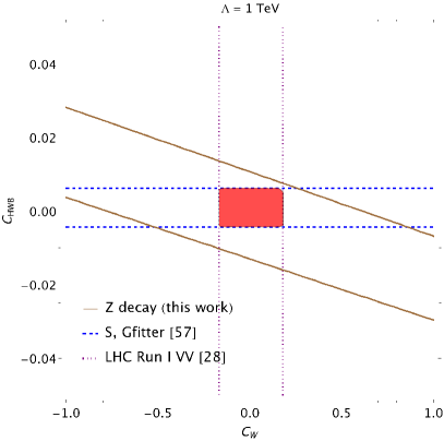
Figure 1: Limits on the coefficients of the operators $\mathcal{O}_{W}$ and $\mathcal{O}_{HWB}$ which contribute to $Z$ decay at one loop and tree level, respectively. All other operators are set to zero, and the region between the solid brown lines is allowed by $Z$ pole measurements given our calculation. For comparison, the region between the dashed blue lines is allowed by the same LEP precision data considering only the impact of the operator $\mathcal{O}_{HWB}$ that modifies the $S$ parameter. The region between the magenta dotted lines is allowed by measurements of $VV$ production at the LHC, to which $\mathcal{O}_{W}$ contributes at tree level. The region in the plane that is allowed by all measurements is shown in red.

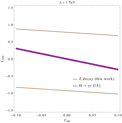
Figure 2: Limits on the coefficients of the operators $\mathcal{O}_{HB}$ and $\mathcal{O}_{HW}$ which contribute to $Z$ decay at one loop. The solid brown lines are as in Fig. 1. (The allowed region is between the lines). For comparison, the region allowed by the more constraining measurement of the $H\to\gamma\gamma$ signal strength is shown in red between the blue dashed lines.

Parameter	SM prediction	Measurement	Correlations
			$g_{L}^{\nu}$	$g_{L}^{\ell}$	$g_{L}^{b}$	$g_{L}^{c}$	$g_{R}^{\ell}$	$g_{R}^{b}$	$g_{R}^{c}$
$g_{L}^{\nu}$	$0.50199\pm 0.00020$	$0.50075\pm 0.00077$	1.00
$g_{L}^{\ell}$	$-0.26919\pm 0.00020$	$-0.26939\pm 0.00022$	-0.32	1.00
$g_{L}^{b}$	$-0.42114\pm 0.00045$	$-0.4182\pm 0.0015$	0.05	-0.27	1.00
$g_{L}^{c}$	$0.34674\pm 0.00017$	$0.3453\pm 0.0036$	-0.02	0.04	-0.09	1.00
$g_{R}^{\ell}$	$0.23208\pm 0.00018$	$0.23186\pm 0.00023$	0.25	0.34	-0.37	0.07	1.00
$g_{R}^{b}$	$0.077420\pm 0.000052$	$0.0962\pm 0.0063$	0.00	-0.33	0.88	-0.14	-0.35	1.00
$g_{R}^{c}$	$-0.15470\pm 0.00011$	$-0.1580\pm 0.0051$	0.00	0.08	-0.17	0.30	0.08	-0.13	1.00

Table 1: LEP and SLD measurements of the effective $Z$ couplings to fermions.

These effective couplings are bounded by LEP measurements at the $Z$ pole. We proceed to take the limits of Schael et al. (2006) on the $Z$-fermion couplings to constrain the SMEFT operators. We minimize a $\chi^{2}$ function constructed using the LEP measurements of the quantities $(g_{L}^{\nu},g_{L}^{e},g_{R}^{e},g_{L}^{u},g_{R}^{u},g_{L}^{b},g_{R}^{b})$ and their correlations shown in Table 1, including the uncertainties on the input parameters. While $Z$ pole measurements constrain all of the operators in Eq. 23, we focus on the implications of our calculation for the operators $\mathcal{O}_{W}$, $\mathcal{O}_{HB}$ and $\mathcal{O}_{HW}$, which do not contribute to $Z$ decay at tree level. We seek to minimize the quantity

$$(\chi^{2})_{\mathrm{LEP}}=\left(\vec{g}_{\mathrm{SMEFT}}-\vec{g}_{\mathrm{exp}}\right)^{\mathrm{T}}V^{-1}\left(\vec{g}_{\mathrm{SMEFT}}-\vec{g}_{\mathrm{exp}}\right)\,,$$ (24)

where $\vec{g}=\left(g_{L}^{\nu},g_{L}^{\ell},g_{L}^{b},g_{L}^{c},g_{R}^{\ell},g_{R}^{b},g_{R}^{c}\right)$ and $V$ is the covariance matrix constructed from the errors and correlations above. We use Eq. 23 together with the SM predictions of Table 1 to calculate $\vec{g}_{\mathrm{SMEFT}}$. Since we set light fermion masses to zero in our SMEFT analysis, the effective couplings for the down (up) quark apply equally to the $b$ ($c$) quark, with the exception of the $b_{L}$ for which top quark corrections apply as specified below Eq. 23.

In Fig. 1, we show the resulting 90% CL limits in 2-dimensional planes of the coefficients of these operators along with that of $\mathcal{O}_{HWB}$, which affects electroweak couplings at tree level. The coefficients of all other operators are set to zero. We compare our results to processes in which the SMEFT operators contribute at tree level. The limit of  Alves et al. (2018), set using LHC Run I data Khachatryan et al. (2016); Aad et al. (2016a, b); Khachatryan et al. (2017), is converted in our notation to

$$-0.17<C_{W}\left(\frac{1~{}\mathrm{TeV}}{\Lambda}\right)^{2}<0.18\,.$$ (25)

For $\mathcal{O}_{W}$, we use the limits of Alves et al. (2018) obtained by using 8 TeV LHC gauge boson pair production in leptonic final states Khachatryan et al. (2016); Aad et al. (2016a, b); Khachatryan et al. (2017).

For $\mathcal{O}_{HB}$ and $\mathcal{O}_{HW}$, we use limits Dawson and Giardino (2018b) from the calculation of $H\to\gamma\gamma$ Hartmann and Trott (2015a); Dedes et al. (2018); Dawson and Giardino (2018b) in the SMEFT, as compared to measurements of $H\to\gamma\gamma$ at Run 1 and 2 of the LHC Aad et al. (2016c); Aaboud et al. (2018); Sirunyan et al. (2018). The SMEFT calculation of $H\to\gamma\gamma$ Dawson and Giardino (2018b) gives,

$$\mu_{\gamma\gamma} = {\Gamma(H\rightarrow\gamma\gamma)\over\Gamma(H\rightarrow\gamma\gamma)\mid_{SM}}$$ (26)

$$= 1-40.15{C_{HB}}\left(\frac{1~{}\mathrm{TeV}}{\Lambda}\right)^{2}-13.08{C_{HW}}\left(\frac{1~{}\mathrm{TeV}}{\Lambda}\right)^{2}+22.40{C_{HWB}}\left(\frac{1~{}\mathrm{TeV}}{\Lambda}\right)^{2}\,.$$

Then, using the average $\mu_{\gamma\gamma}=1.09\pm 0.10$ of current LHC Higgs measurements Aad et al. (2016c); Aaboud et al. (2018); Sirunyan et al. (2018), we find,

$$-0.003<\mid{C_{HB}}\left(\frac{1~{}\mathrm{TeV}}{\Lambda}\right)^{2}+.33{C_{HW}}\left(\frac{1~{}\mathrm{TeV}}{\Lambda}\right)^{2}\ -.55{C_{HWB}}\left(\frac{1~{}\mathrm{TeV}}{\Lambda}\right)^{2}\mid<0.007\,,$$ (27)

or taking only one non-zero coupling at a time with the conservative bound $|\mu_{\gamma\gamma}-1|<0.29$,

$$\begin{split}\left|C_{HB}\left(\frac{1~{}\mathrm{TeV}}{\Lambda}\right)^{2}\right|&<0.007\\ \left|C_{HW}\left(\frac{1~{}\mathrm{TeV}}{\Lambda}\right)^{2}\right|&<0.02\,.\end{split}$$ (28)

$\mathcal{O}_{HWB}$ corresponds to the oblique parameter $S$ Peskin and Takeuchi (1990, 1992), whose limit we take from the Gfitter collaborationHaller et al. (2018) of $S=0.04\pm 0.11$ to set the $2\sigma$ bound,

$$-0.004<C_{HWB}<0.006\,.$$ (29)

The existing bounds in Fig. 2 are stronger than those that we obtain directly from $Z$ pole measurements. Nevertheless, they provide complementary information, and in particular in Fig. 2, the interplay between the limits on $C_{W}$ and $C_{HWB}$ demonstrates the power of electroweak precision measurements to constrain couplings that only contribute at loop level. In the case of the operators $C_{HB}$ and $C_{HW}$ which directly affect $H\to\gamma\gamma$, Higgs precision is already significantly more effective than $Z$ pole measurements in setting limits, due to the loop suppression of these operators’ contributions to $Z$ decay.

IV Conclusions

Precision measurements of electroweak physics will eventually necessitate higher order calculations of BSM contributions. The SMEFT framework takes a general approach to potential new UV physics by parametrizing its effects in terms of higher dimension operators involving the SM fields. In this work, we have furthered the applicability of the SMEFT to probe new physics by considering the one loop corrections to $Z$ decay from operators which contribute to gauge boson production.

While the contributions of the operators $\mathcal{O}_{W}$, $\mathcal{O}_{HB}$ and $\mathcal{O}_{HW}$ are small relative to those of the operators that modify the $Z$ coupling to fermions at tree level, the relative size of all of the SMEFT operators is fixed by the new physics. In particular, integrating out a heavy SM singlet scalar could naturally give these operators without changing the leading $Z$ couplings to the fermions de Blas et al. (2018). In such a scenario, it would be essential to have the higher order contributions of the BSM physics to all possible processes. In this regard our calculation provides a useful prediction, relating the effects of new physics in $Z$ decay to those in other electroweak processes provided the states responsible for deviations from the SM are heavy enough to be integrated out.

A full calculation of $Z$ decay at one loop in the SMEFT would provide even more complete information about the influence of higher dimensional operators on $Z$ physics. With this as well as other higher order calculations of electroweak processes, in the future a global fit at NLO in the SMEFT could be performed to bound the sizes of all possible dimension-$6$ SMEFT operators.

Appendix A UV poles

The cancellation of UV poles follows from the individual contributions: Numerically with $\Lambda=1~{}\mathrm{TeV}$, the pieces are as follows.

$$\frac{\partial M_{0}}{\partial C_{HWB}}\delta C_{HWB} =\frac{1}{\epsilon}\Big{\{}Q_{f}\left(\left(2.7\times 10^{-5}\right)C_{HB}+\left(2.7\times 10^{-5}\right)C_{HW}+\left(4.6\times 10^{-4}\right)C_{HWB}+\left(2.6\times 10^{-5}\right)C_{W}\right)\Big{\}}+\mathcal{O}(\epsilon^{0})$$

$$\frac{\partial M_{0}}{\partial G_{\mu}}\delta G_{\mu} =\frac{1}{\epsilon}\Big{\{}\left(2.1\times 10^{-5}\right)\left(Q_{f}(C_{HWB}+8.8)-40T_{3}^{f}\right)(\xi-5.5)\Big{\}}+\mathcal{O}(\epsilon^{0})$$

$$\frac{\partial M_{0}}{\partial M_{Z}^{2}}\delta M_{Z}^{2} =\frac{1}{\epsilon}\Big{\{}Q_{f}\big{(}\left(-1.4\times 10^{-4}\right)\xi C_{HW}-\left(3.2\times 10^{-4}\right)C_{HW}-\left(6.7\times 10^{-4}\right)C_{HWB}+\left(7.7\times 10^{-4}\right)C_{W}$$

$$\quad+C_{HB}\left(\left(-3.9\times 10^{-5}\right)\xi-9.1\times 10^{-5}\right)-\left(1.4\times 10^{-6}\right)C_{HWB}\xi-\left(1.5\times 10^{-3}\right)\xi+1.2\times 10^{-2}\big{)}$$

$$\quad+T_{3}^{f}\big{(}\left(7.7\times 10^{-5}\right)\xi C_{HW}+\left(1.8\times 10^{-4}\right)C_{HW}+\left(5.3\times 10^{-5}\right)C_{HWB}-\left(4.3\times 10^{-4}\right)C_{W}$$

$$\quad+C_{HB}\left(\left(2.2\times 10^{-5}\right)\xi+5.1\times 10^{-5}\right)+\left(4.1\times 10^{-5}\right)C_{HWB}\xi+\left(8.2\times 10^{-4}\right)\xi-6.5\times 10^{-3}\big{)}\Big{\}}+\mathcal{O}(\epsilon^{0})$$

$$\frac{\partial M_{0}}{\partial M_{W}^{2}}\delta M_{W}^{2} =\frac{Q_{f}}{\epsilon}\Big{\{}\left(-9.2\times 10^{-4}\right)C_{W}+C_{HWB}\left(5.3\times 10^{-4}-\left(5.2\times 10^{-5}\right)\xi\right)+C_{HW}\left(\left(1.5\times 10^{-4}\right)\xi+3.0\times 10^{-4}\right)$$

$$\quad+\left(1.3\times 10^{-3}\right)\xi-1.2\times 10^{-2}\Big{\}}+\mathcal{O}(\epsilon^{0})$$

$$-M_{\gamma}\frac{\Pi_{\gamma Z}\left(M_{Z}^{2}\right)}{M_{Z}^{2}} =\frac{Q_{f}}{\epsilon}\Big{\{}\left(3.7\times 10^{-5}\right)\xi C_{HWB}-\left(2.3\times 10^{-4}\right)C_{HWB}+\left(1.9\times 10^{-4}\right)C_{W}+C_{HW}\big{(}\left(-3.5\times 10^{-5}\right)\xi$$

$$\quad-5.2\times 10^{-5}\big{)}+C_{HB}\left(\left(3.5\times 10^{-5}\right)\xi+5.2\times 10^{-5}\right)-\left(1.7\times 10^{-4}\right)\xi+1.3\times 10^{-3}\Big{\}}+\mathcal{O}(\epsilon^{0})$$

$$\frac{Z_{Z}}{2}M_{0} =\frac{1}{\epsilon}\Big{\{}T_{3}^{f}\big{(}\left(-7.7\times 10^{-5}\right)\xi C_{HW}-\left(1.8\times 10^{-4}\right)C_{HW}-\left(1.3\times 10^{-4}\right)C_{HWB}+\left(3.2\times 10^{-4}\right)C_{W}$$

$$\quad+C_{HB}\left(\left(-2.2\times 10^{-5}\right)\xi-5.1\times 10^{-5}\right)-\left(6.7\times 10^{-5}\right)C_{HWB}\xi-\left(7.8\times 10^{-4}\right)\xi-3.1\times 10^{-4}\big{)}$$

$$\quad+Q_{f}\big{(}\left(1.7\times 10^{-5}\right)\xi C_{HW}+\left(4.0\times 10^{-5}\right)C_{HW}+\left(2.1\times 10^{-5}\right)C_{HWB}-\left(7.0\times 10^{-5}\right)C_{W}$$

$$\quad+C_{HB}\left(\left(4.9\times 10^{-6}\right)\xi+1.1\times 10^{-5}\right)-\left(4.7\times 10^{-6}\right)C_{HWB}\xi+\left(1.7\times 10^{-4}\right)\xi+6.9\times 10^{-5}\big{)}\Big{\}}+\mathcal{O}(\epsilon^{0})$$

$$Z_{f}M_{0} =\frac{\xi}{\epsilon}\Big{\{}Q_{f}^{3}\left(1.3\times 10^{-4}-\left(4.3\times 10^{-5}\right)C_{HWB}\right)+Q_{f}^{2}T_{3}^{f}\left(\left(1.9\times 10^{-4}\right)C_{HWB}-8.3\times 10^{-4}\right)$$

$$\quad+Q_{f}T_{3}^{f2}\left(2.6\times 10^{-3}-\left(3.0\times 10^{-4}\right)C_{HWB}\right)-\left(1.6\times 10^{-3}\right)T_{3}^{f}\Big{\}}+\mathcal{O}(\epsilon^{0})$$

$$M_{1} =\frac{1}{\epsilon}\Big{\{}Q_{f}^{3}\left(\left(4.3\times 10^{-5}\right)C_{HWB}-1.3\times 10^{-4}\right)\xi+Q_{f}T_{3}^{f2}\big{(}\left(3.0\times 10^{-4}\right)C_{HWB}-2.6\times 10^{-3}\big{)}\xi$$

$$\quad+T_{3}^{f}\big{(}\left(8.3\times 10^{-4}\right)\xi Q_{f}^{2}+\left(1.2\times 10^{-4}\right)C_{W}+\left(2.4\times 10^{-3}\right)\xi+C_{HWB}\big{(}\left(-1.9\times 10^{-4}\right)\xi Q_{f}^{2}$$

$$\quad+\left(2.5\times 10^{-5}\right)\xi+7.6\times 10^{-5}\big{)}+2.3\times 10^{-3}\big{)}\Big{\}}+\mathcal{O}(\epsilon^{0})$$

The sum vanishes for any given fermion.

Appendix B $2$-point functions

In this appendix, we show the two-point functions in $R_{\xi}$ gauge due to the SMEFT operators that also contribute to gauge boson pair production. Previous results for the gauge boson two-point functions in other operator bases appear in Alam et al. (1998); Chen et al. (2014).

In $D=4-2\epsilon$ dimensions, the two-point function for a massless fermion with weak isospin $T_{3}^{f}$ and charge $Q_{f}$ is

$$\Sigma(p) =\frac{1}{8\pi^{2}}\Bigg{(}\frac{2\sqrt{2}A_{0}(M_{W}^{2})G_{\mu}T_{3}^{f2}\left((D-2)M_{W}^{2}-p^{2}\right)}{p^{2}}+2\sqrt{2}A_{0}(M_{W}^{2}\xi)G_{\mu}T_{3}^{f2}$$

$$\quad+\frac{1}{M_{Z}^{4}p^{2}}\bigg{(}A_{0}(M_{Z}^{2})\left((D-2)M_{Z}^{2}-p^{2}\right)\left(M_{W}^{2}Q_{f}+M_{Z}^{2}(T_{3}^{f}-Q_{f})\right)\Big{(}\sqrt{2}G_{\mu}\left(M_{W}^{2}Q_{f}+M_{Z}^{2}(T_{3}^{f}-Q_{f})\right)$$

$$\quad+2M_{W}Q_{f}C_{HWB}\sqrt{M_{Z}^{2}-M_{W}^{2}}\Big{)}\bigg{)}$$

$$\quad-\frac{A_{0}(M_{Z}^{2}\beta)(D-2)M_{W}^{2}Q_{f}^{2}\left(\sqrt{2}G_{\mu}(M_{W}-M_{Z})(M_{W}+M_{Z})+2M_{W}C_{HWB}\sqrt{M_{Z}^{2}-M_{W}^{2}}\right)}{M_{Z}^{2}p^{2}}$$

$$\quad+\frac{A_{0}(M_{Z}^{2}\xi)\left(M_{W}^{2}Q_{f}+M_{Z}^{2}(T_{3}^{f}-Q_{f})\right)\left(\sqrt{2}G_{\mu}\left(M_{W}^{2}Q_{f}+M_{Z}^{2}(T_{3}^{f}-Q_{f})\right)+2M_{W}Q_{f}C_{HWB}\sqrt{M_{Z}^{2}-M_{W}^{2}}\right)}{M_{Z}^{4}}$$

$$\quad-\frac{B_{0}(0,M_{Z}^{2}\beta,M_{Z}^{2}\beta)M_{W}^{2}(\xi-1)Q_{f}^{2}\left(\sqrt{2}G_{\mu}(M_{W}-M_{Z})(M_{W}+M_{Z})+2M_{W}C_{HWB}\sqrt{M_{Z}^{2}-M_{W}^{2}}\right)}{M_{Z}^{2}}$$

$$\quad+\frac{2\sqrt{2}B_{0}(p^{2},0,M_{W}^{2})G_{\mu}T_{3}^{f2}\left(p^{2}-M_{W}^{2}\right)\left((D-2)M_{W}^{2}+p^{2}\right)}{p^{2}}-2\sqrt{2}B_{0}(p^{2},0,M_{W}^{2}\xi)G_{\mu}T_{3}^{f2}\left(p^{2}-M_{W}^{2}\xi\right)$$

$$\quad-\frac{1}{M_{Z}^{4}p^{2}}\bigg{(}B_{0}(p^{2},0,M_{Z}^{2})(M_{Z}-p)(M_{Z}+p)\left((D-2)M_{Z}^{2}+p^{2}\right)\left(M_{W}^{2}Q_{f}+M_{Z}^{2}(T_{3}^{f}-Q_{f})\right)\Big{(}\sqrt{2}G_{\mu}\big{(}M_{W}^{2}Q_{f}$$

$$\quad+M_{Z}^{2}(T_{3}^{f}-Q_{f})\big{)}+2M_{W}Q_{f}C_{HWB}\sqrt{M_{Z}^{2}-M_{W}^{2}}\Big{)}\bigg{)}$$

$$\quad+\frac{1}{M_{Z}^{2}p^{2}}\bigg{(}B_{0}(p^{2},0,M_{Z}^{2}\beta)M_{W}^{2}Q_{f}^{2}\left(\beta(D-2)M_{Z}^{2}-p^{2}(D+\xi-3)\right)\Big{(}\sqrt{2}G_{\mu}(M_{W}-M_{Z})(M_{W}+M_{Z})$$

$$\quad+2M_{W}C_{HWB}\sqrt{M_{Z}^{2}-M_{W}^{2}}\Big{)}\bigg{)}$$

$$\quad+\frac{1}{M_{Z}^{4}}\bigg{(}B_{0}(p^{2},0,M_{Z}^{2}\xi)\left(M_{Z}^{2}\xi-p^{2}\right)\left(M_{W}^{2}Q_{f}+M_{Z}^{2}(T_{3}^{f}-Q_{f})\right)\Big{(}\sqrt{2}G_{\mu}\left(M_{W}^{2}Q_{f}+M_{Z}^{2}(T_{3}^{f}-Q_{f})\right)$$

$$\quad+2M_{W}Q_{f}C_{HWB}\sqrt{M_{Z}^{2}-M_{W}^{2}}\Big{)}\bigg{)}+\frac{1}{M_{Z}^{2}}\bigg{(}C_{0}(0,p^{2},p^{2},M_{Z}^{2}\beta,M_{Z}^{2}\beta,0)M_{W}^{2}(\xi-1)Q_{f}^{2}\left(p^{2}-\beta M_{Z}^{2}\right)$$

$$\quad\times\left(\sqrt{2}G_{\mu}(M_{W}-M_{Z})(M_{W}+M_{Z})+2M_{W}C_{HWB}\sqrt{M_{Z}^{2}-M_{W}^{2}}\right)\bigg{)}\Bigg{)}$$ (30)

We have regulated IR divergences with a photon of mass $M_{Z}\beta$, and use standard FeynCalc notation Mertig et al. (1991) for the Passarino-Veltman functions.

This leads to the wave function renormalization

$$Z_{f} =\frac{1}{8\pi^{2}\epsilon}\Bigg{(}\frac{1}{M_{Z}^{2}}\bigg{(}Q_{f}^{2}\left(\sqrt{2}G_{\mu}(M_{W}-M_{Z})(M_{W}+M_{Z})+2M_{W}C_{HWB}\sqrt{M_{Z}^{2}-M_{W}^{2}}\right)\big{(}2\xi\epsilon\big{(}M_{W}^{2}(\log(\beta)-\log(\xi))$$

$$\quad+M_{Z}^{2}(\log(M_{Z}^{2}/\mu^{2})+\log(\pi\xi))\big{)}+2M_{W}^{2}(\xi-1)\epsilon+M_{Z}^{2}((2(\gamma-1)\xi+3)\epsilon-2\xi)\big{)}\bigg{)}$$

$$\quad-2Q_{f}T_{3}^{f}\left(\sqrt{2}G_{\mu}(M_{W}-M_{Z})(M_{W}+M_{Z})+M_{W}C_{HWB}\sqrt{M_{Z}^{2}-M_{W}^{2}}\right)(2\xi\epsilon(2\log(M_{Z}^{2}/\mu^{2})+\log(\pi\xi))-2\xi$$

$$\quad+(2(\gamma-1)\xi+3)\epsilon)-\sqrt{2}G_{\mu}T_{3}^{f2}\big{(}\left(2M_{W}^{2}+M_{Z}^{2}\right)(2\xi\epsilon(\log(\pi\xi))+2\xi((\gamma-1)\epsilon-1)+3\epsilon)+4M_{W}^{2}\xi\epsilon\log(M_{W}^{2}/\mu^{2})$$

$$\quad+2M_{Z}^{2}\xi\epsilon\log(M_{Z}^{2}/\mu^{2})\big{)}\Bigg{)}$$ (31)

For the $b_{L}$, there are corrections proportional to the top mass, leading to an additional wave function renormalization which in Feynman gauge is

$$Z_{b_{L}}=Z_{f}\left(Q_{f}=-\frac{1}{3},T_{3}^{f}=-\frac{1}{2}\right)+\frac{G_{\mu}M_{T}^{2}\left(2\epsilon\log\left(\frac{\mu^{2}}{M_{W}^{2}}\right)-2\gamma\epsilon+\epsilon-2\epsilon\log\pi+2\right)}{16\sqrt{2}\pi^{2}\epsilon}$$ (32)

The transverse $W$ two-point function is

$$\Pi_{WW}^{T}(p^{2}) =\frac{1}{16p^{2}\pi^{2}}\Bigg{(}-\frac{18\sqrt{2}B_{0}(p^{2},0,0)(D-2)G_{\mu}M_{W}^{2}p^{4}}{D-1}-\frac{1}{(D-1)M_{Z}^{2}}\bigg{(}C_{0}(0,p^{2},p^{2},0,0,M_{W}^{2}\xi)\left(M_{W}^{4}-p^{4}\right)$$

$$\quad\times\left(\sqrt{2}G_{\mu}(M_{W}-M_{Z})(M_{W}+M_{Z})+2M_{W}\sqrt{M_{Z}^{2}-M_{W}^{2}}C_{HWB}\right)(\xi-1)\left(p^{2}-M_{W}^{2}\xi\right)^{2}\bigg{)}$$

$$\quad-\frac{6\sqrt{2}A_{0}(M_{T}^{2})G_{\mu}M_{W}^{2}\left(M_{T}^{2}-(D-2)p^{2}\right)}{D-1}+\frac{6\sqrt{2}B_{0}(p^{2},0,M_{T}^{2})G_{\mu}M_{W}^{2}(M_{T}-p)(M_{T}+p)\left(M_{T}^{2}+(D-2)p^{2}\right)}{D-1}$$

$$\quad-\frac{1}{D-1}\bigg{(}B_{0}(p^{2},M_{H}^{2},M_{W}^{2})M_{W}^{2}\Big{(}8(D-1)\left(-M_{H}^{2}+M_{W}^{2}+p^{2}\right)C_{HW}p^{2}$$

$$\quad+\sqrt{2}G_{\mu}\left(p^{4}-2\left(M_{H}^{2}+(3-2D)M_{W}^{2}\right)p^{2}+\left(M_{H}^{2}-M_{W}^{2}\right)^{2}\right)\Big{)}\bigg{)}+\frac{1}{D-1}\bigg{(}A_{0}(M_{H}^{2})\Big{(}\sqrt{2}G_{\mu}M_{W}^{2}\big{(}M_{H}^{2}-M_{W}^{2}$$

$$\quad-(D-2)p^{2}\big{)}-2(D-1)p^{2}\left(4M_{W}^{2}+p^{2}\right)C_{HW}\Big{)}\bigg{)}-\frac{1}{(D-1)M_{Z}^{4}}\bigg{(}B_{0}(p^{2},M_{W}^{2},M_{Z}^{2})M_{W}(M_{W}+M_{Z}-p)(M_{W}+$$

$$\quad M_{Z}+p)\left((M_{W}-M_{Z})^{2}-p^{2}\right)\Big{(}36\sqrt[4]{2}(D-2)\sqrt{G_{\mu}}M_{W}^{2}M_{Z}^{2}C_{W}p^{2}+\sqrt{2}G_{\mu}M_{W}\big{(}M_{W}^{4}$$

$$\quad+2(2D-3)\left(M_{Z}^{2}+p^{2}\right)M_{W}^{2}+M_{Z}^{4}+p^{4}+2(2D-3)M_{Z}^{2}p^{2}\big{)}+2\sqrt{M_{Z}^{2}-M_{W}^{2}}\big{(}M_{W}^{4}+(2D-3)\left(M_{Z}^{2}+2p^{2}\right)M_{W}^{2}$$

$$\quad+p^{4}+(2D-3)M_{Z}^{2}p^{2}\big{)}C_{HWB}\Big{)}\bigg{)}+\frac{1}{(D-1)M_{Z}^{2}}\bigg{(}C_{0}(0,p^{2},p^{2},0,0,M_{W}^{2})\left(M_{W}^{2}-p^{2}\right)^{2}\big{(}M_{W}^{4}$$

$$\quad+2(2D-3)p^{2}M_{W}^{2}+p^{4}\big{)}\left(\sqrt{2}G_{\mu}\left(M_{Z}^{2}-M_{W}^{2}\right)-2M_{W}\sqrt{M_{Z}^{2}-M_{W}^{2}}C_{HWB}\right)(\xi-1)\bigg{)}$$

$$\quad+\frac{1}{(D-1)M_{Z}^{4}}\bigg{(}B_{0}(p^{2},M_{W}^{2}\xi,M_{Z}^{2}\xi)M_{W}\left(M_{W}^{4}-p^{4}\right)\left(\sqrt{2}G_{\mu}M_{W}+2\sqrt{M_{Z}^{2}-M_{W}^{2}}C_{HWB}\right)$$

$$\quad\times\left(p^{4}-2\left(M_{W}^{2}+M_{Z}^{2}\right)\xi p^{2}+\left(M_{W}^{2}-M_{Z}^{2}\right)^{2}\xi^{2}\right)\bigg{)}+\frac{1}{(D-1)M_{Z}^{4}}\bigg{(}B_{0}(p^{2},M_{W}^{2},M_{Z}^{2}\xi)M_{W}\left(M_{W}^{2}-p^{2}\right)^{2}$$

$$\quad\times\left(\sqrt{2}G_{\mu}M_{W}+2\sqrt{M_{Z}^{2}-M_{W}^{2}}C_{HWB}\right)\left(M_{W}^{4}+\left((4D-6)p^{2}-2M_{Z}^{2}\xi\right)M_{W}^{2}+\left(p^{2}-M_{Z}^{2}\xi\right)^{2}\right)\bigg{)}$$

$$\quad-\frac{1}{D-1}\bigg{(}A_{0}(M_{W}^{2}\xi)\Big{(}2\left(2(D-1)C_{HW}p^{4}+M_{W}\sqrt{M_{Z}^{2}-M_{W}^{2}}C_{HWB}p^{2}-M_{W}^{3}\sqrt{M_{Z}^{2}-M_{W}^{2}}C_{HWB}\right)$$

$$\quad+\sqrt{2}G_{\mu}\left((\xi-1)M_{W}^{4}-2p^{2}(D+\xi-3)M_{W}^{2}+p^{4}(4D+\xi-7)\right)\Big{)}\bigg{)}-\frac{1}{(1-D)M_{Z}^{2}}\bigg{(}2B_{0}(p^{2},0,M_{W}^{2})$$

$$\quad\times\Big{(}18\sqrt[4]{2}(D-2)\sqrt{G_{\mu}}M_{W}(M_{W}-M_{Z})(M_{W}+M_{Z})(M_{W}-p)^{2}p^{2}C_{W}(M_{W}+p)^{2}$$

$$\quad+\sqrt{2}G_{\mu}(M_{W}-M_{Z})(M_{W}+M_{Z})\left(M_{W}^{2}+p^{2}\right)\left((2D+\xi-4)M_{W}^{4}-2p^{2}(4D+\xi-6)M_{W}^{2}+p^{4}(2D+\xi-4)\right)$$

$$\quad+M_{W}\sqrt{M_{Z}^{2}-M_{W}^{2}}\left(M_{W}^{2}+p^{2}\right)C_{HWB}\left((2D+2\xi-5)M_{W}^{4}-2p^{2}(6D+2\xi-9)M_{W}^{2}+p^{4}(2D+2\xi-5)\right)\Big{)}\bigg{)}$$

$$\quad-\frac{1}{(D-1)M_{Z}^{2}}\bigg{(}2B_{0}(p^{2},0,M_{W}^{2}\xi)(M_{W}-p)(M_{W}+p)\bigg{(}\sqrt{2}G_{\mu}(M_{W}-M_{Z})(M_{W}+M_{Z})\Big{(}\xi M_{W}^{4}-p^{2}\big{(}\xi^{2}+2\xi$$

$$\quad+2D-3\big{)}M_{W}^{2}-p^{4}(2D+\xi-4)\Big{)}-M_{W}\sqrt{M_{Z}^{2}-M_{W}^{2}}C_{HWB}\big{(}(\xi-2)\xi M_{W}^{4}+2p^{2}\left(\xi^{2}+D(\xi+2)-3\right)M_{W}^{2}$$

$$\quad+p^{4}(2D+2\xi-5)\big{)}\bigg{)}\bigg{)}+\frac{1}{(D-1)M_{Z}^{4}}\bigg{(}A_{0}(M_{Z}^{2}\xi)\Big{(}\sqrt{2}G_{\mu}\big{(}(\xi+1)M_{W}^{6}+\left(4(D-2)p^{2}-2M_{Z}^{2}\xi\right)M_{W}^{4}$$

$$\quad+\left(2M_{Z}^{2}p^{2}\xi-p^{4}(4D+\xi-7)\right)M_{W}^{2}-(D-1)M_{Z}^{4}p^{2}\big{)}M_{W}^{2}+2\Big{(}-(D-1)M_{Z}^{4}C_{HW}p^{4}$$

$$\quad+2M_{W}^{3}M_{Z}^{2}\sqrt{M_{Z}^{2}-M_{W}^{2}}\left(p^{2}-M_{W}^{2}\right)C_{HWB}\xi+M_{W}^{3}\sqrt{M_{Z}^{2}-M_{W}^{2}}(M_{W}-p)(M_{W}+p)C_{HWB}\big{(}(\xi+1)M_{W}^{2}$$

$$\quad+p^{2}(4D+\xi-7)\big{)}\Big{)}\Big{)}\bigg{)}+\frac{1}{D-1}\bigg{(}A_{0}(M_{W}^{2})\Big{(}36\sqrt[4]{2}(D-2)\sqrt{G_{\mu}}M_{W}C_{W}p^{4}$$

$$\quad+2M_{W}\left((3-2D)\sqrt{M_{Z}^{2}-M_{W}^{2}}C_{HWB}M_{W}^{2}+4(D-1)p^{2}C_{HW}M_{W}+(3-2D)\sqrt{M_{Z}^{2}-M_{W}^{2}}p^{2}C_{HWB}\right)$$

$$\quad+\sqrt{2}G_{\mu}\left((\xi+1)M_{W}^{4}-M_{H}^{2}M_{W}^{2}-\left(M_{Z}^{2}+2p^{2}(2(D-3)D+\xi+3)\right)M_{W}^{2}+p^{4}(4D+\xi-7)\right)\Big{)}\bigg{)}$$

$$\quad-\frac{1}{(D-1)M_{Z}^{4}}\bigg{(}A_{0}(M_{Z}^{2})M_{W}\Big{(}36\sqrt[4]{2}(D-2)\sqrt{G_{\mu}}M_{W}^{2}M_{Z}^{2}\left(M_{W}^{2}-M_{Z}^{2}-p^{2}\right)C_{W}p^{2}+\sqrt{2}G_{\mu}M_{W}\big{(}(\xi+1)M_{W}^{6}$$

$$\quad+2\left(2(D-2)\left(M_{Z}^{2}+p^{2}\right)-M_{Z}^{2}\xi\right)M_{W}^{4}+\left((9-4D)M_{Z}^{4}+2p^{2}\left(2(D-2)^{2}+\xi\right)M_{Z}^{2}-p^{4}(4D+\xi-7)\right)M_{W}^{2}$$

$$\quad-M_{Z}^{4}\left(M_{Z}^{2}+p^{2}\right)\big{)}+2\sqrt{M_{Z}^{2}-M_{W}^{2}}C_{HWB}\big{(}(\xi+1)M_{W}^{6}+\left((2D-\xi-5)M_{Z}^{2}+4(D-2)p^{2}\right)M_{W}^{4}$$

$$\quad+\left(-2(D-2)M_{Z}^{4}+p^{2}(2D(2D-7)+\xi+13)M_{Z}^{2}-p^{4}(4D+\xi-7)\right)M_{W}^{2}-2(D-1)M_{Z}^{4}p^{2}\big{)}\Big{)}\bigg{)}$$

$$\quad+\frac{1}{(D-1)M_{Z}^{4}}\bigg{(}B_{0}(p^{2},M_{Z}^{2},M_{W}^{2}\xi)M_{W}(M_{W}-p)(M_{W}+p)\Big{(}-\sqrt{2}G_{\mu}M_{W}\left(M_{W}^{2}-2M_{Z}^{2}+p^{2}\right)\big{(}M_{Z}^{4}+$$

$$\quad\left((4D-6)p^{2}-2M_{W}^{2}\xi\right)M_{Z}^{2}+\left(p^{2}-M_{W}^{2}\xi\right)^{2}\big{)}-2\sqrt{M_{Z}^{2}-M_{W}^{2}}C_{HWB}\big{(}\xi^{2}M_{W}^{6}-\xi\left(M_{Z}^{2}(\xi+2)-p^{2}(\xi-2)\right)M_{W}^{4}$$

$$\quad+\left((2\xi+1)M_{Z}^{4}+2p^{2}(-\xi+D(\xi+2)-3)M_{Z}^{2}+p^{4}(1-2\xi)\right)M_{W}^{2}-M_{Z}^{6}+p^{6}+(2D-5)M_{Z}^{2}p^{4}$$

$$\quad+3(3-2D)M_{Z}^{4}p^{2}\big{)}\Big{)}\bigg{)}\Bigg{)}$$ (33)

which yields the mass shift

$$\delta M_{W}^{2} =\Pi_{WW}^{T}(M_{W}^{2})$$

$$=\frac{1}{16\pi^{2}}\Bigg{(}\frac{A_{0}(M_{H}^{2})\left(\sqrt{2}G_{\mu}\left(M_{H}^{2}-(D-1)M_{W}^{2}\right)-10(D-1)M_{W}^{2}C_{HW}\right)}{D-1}$$

$$\quad-\frac{6\sqrt{2}A_{0}(M_{T}^{2})G_{\mu}\left(M_{T}^{2}-(D-2)M_{W}^{2}\right)}{D-1}-\frac{1}{D-1}\bigg{(}A_{0}(M_{W}^{2})\bigg{(}-36\sqrt[4]{2}(D-2)\sqrt{G_{\mu}}M_{W}^{3}C_{W}$$

$$\quad+\sqrt{2}G_{\mu}\left(4(D-3)(D-1)M_{W}^{2}+M_{H}^{2}+M_{Z}^{2}\right)+4M_{W}\left((2D-3)C_{HWB}\sqrt{M_{Z}^{2}-M_{W}^{2}}-2(D-1)M_{W}C_{HW}\right)\bigg{)}\bigg{)}$$

$$\quad-2A_{0}(M_{W}^{2}\xi)M_{W}^{2}\left(\sqrt{2}G_{\mu}+2C_{HW}\right)+\frac{1}{(D-1)M_{Z}^{2}}\bigg{(}A_{0}(M_{Z}^{2})\Big{(}36\sqrt[4]{2}(D-2)\sqrt{G_{\mu}}M_{W}^{3}M_{Z}^{2}C_{W}$$

$$\quad+\sqrt{2}G_{\mu}\left(-4(D-2)(D-1)M_{W}^{4}+4(D-2)M_{W}^{2}M_{Z}^{2}+M_{Z}^{4}\right)-4M_{W}C_{HWB}\sqrt{M_{Z}^{2}-M_{W}^{2}}\big{(}2(D-2)(D-1)M_{W}^{2}$$

$$\quad+(3-2D)M_{Z}^{2}\big{)}\Big{)}\bigg{)}-A_{0}(M_{Z}^{2}\xi)M_{W}^{2}\left(\sqrt{2}G_{\mu}+2C_{HW}\right)-\frac{18\sqrt{2}B_{0}(M_{W}^{2},0,0)(D-2)G_{\mu}M_{W}^{4}}{D-1}$$

$$\quad+\frac{6\sqrt{2}B_{0}(M_{W}^{2},0,M_{T}^{2})G_{\mu}(M_{T}-M_{W})(M_{T}+M_{W})\left((D-2)M_{W}^{2}+M_{T}^{2}\right)}{D-1}+\frac{1}{M_{Z}^{2}}\bigg{(}16B_{0}(M_{W}^{2},0,M_{W}^{2})M_{W}^{4}$$

$$\quad\times\left(\sqrt{2}G_{\mu}\left(M_{Z}^{2}-M_{W}^{2}\right)-2M_{W}C_{HWB}\sqrt{M_{Z}^{2}-M_{W}^{2}}\right)\bigg{)}-\frac{1}{D-1}\bigg{(}B_{0}(M_{W}^{2},M_{H}^{2},M_{W}^{2})\Big{(}\sqrt{2}G_{\mu}\big{(}4(D-1)M_{W}^{4}$$

$$\quad+M_{H}^{4}-4M_{H}^{2}M_{W}^{2}\big{)}-8(D-1)M_{W}^{2}C_{HW}\left(M_{H}^{2}-2M_{W}^{2}\right)\Big{)}\bigg{)}+\frac{1}{(D-1)M_{Z}^{2}}\bigg{(}B_{0}(M_{W}^{2},M_{W}^{2},M_{Z}^{2})\left(4M_{W}^{2}-M_{Z}^{2}\right)$$

$$\quad\times\Big{(}36\sqrt[4]{2}(D-2)\sqrt{G_{\mu}}M_{W}^{3}M_{Z}^{2}C_{W}+\sqrt{2}G_{\mu}\left(4(D-1)M_{W}^{4}+4(2D-3)M_{W}^{2}M_{Z}^{2}+M_{Z}^{4}\right)$$

$$\quad+4M_{W}C_{HWB}\sqrt{M_{Z}^{2}-M_{W}^{2}}\left(2(D-1)M_{W}^{2}+(2D-3)M_{Z}^{2}\right)\Big{)}\bigg{)}\Bigg{)}$$ (34)

The transverse $Z$ two-point function is

$$\Pi_{ZZ}^{T}(p^{2}) =\frac{1}{48\pi^{2}}\Bigg{(}-\frac{1}{(D-1)M_{Z}^{2}}\bigg{(}B_{0}(p^{2},0,0)(D-2)\Big{(}\sqrt{2}G_{\mu}\left(160M_{W}^{4}-200M_{Z}^{2}M_{W}^{2}+103M_{Z}^{4}\right)$$

$$\quad+40M_{W}\left(8M_{W}^{2}-5M_{Z}^{2}\right)\sqrt{M_{Z}^{2}-M_{W}^{2}}C_{HWB}\Big{)}p^{2}\bigg{)}+\frac{1}{(D-1)M_{Z}^{2}}\bigg{(}2A_{0}(M_{T}^{2})(D-2)\Big{(}\sqrt{2}G_{\mu}\big{(}32M_{W}^{4}$$

$$\quad-40M_{Z}^{2}M_{W}^{2}+17M_{Z}^{4}\big{)}+8M_{W}\left(8M_{W}^{2}-5M_{Z}^{2}\right)\sqrt{M_{Z}^{2}-M_{W}^{2}}C_{HWB}\Big{)}\bigg{)}-\frac{1}{(1-D)M_{Z}^{2}}\bigg{(}B_{0}(p^{2},M_{T}^{2},M_{T}^{2})$$

$$\quad\times\Big{(}\sqrt{2}G_{\mu}\left(2M_{T}^{2}\left(-64M_{W}^{4}+80M_{Z}^{2}M_{W}^{2}+(9D-43)M_{Z}^{4}\right)-(D-2)\left(32M_{W}^{4}-40M_{Z}^{2}M_{W}^{2}+17M_{Z}^{4}\right)p^{2}\right)$$

$$\quad-8M_{W}\left(8M_{W}^{2}-5M_{Z}^{2}\right)\sqrt{M_{Z}^{2}-M_{W}^{2}}\left(4M_{T}^{2}+(D-2)p^{2}\right)C_{HWB}\Big{)}\bigg{)}-\frac{1}{M_{Z}^{2}}\bigg{(}3A_{0}(M_{Z}^{2}\xi)\Big{(}\sqrt{2}G_{\mu}M_{Z}^{4}+2p^{2}$$

$$\quad\times\Big{(}(C_{HW}-C_{HB})M_{W}^{2}+\sqrt{M_{Z}^{2}-M_{W}^{2}}C_{HWB}M_{W}+M_{Z}^{2}C_{HB}\Big{)}\Big{)}\bigg{)}+\frac{1}{(D-1)M_{Z}^{2}}\bigg{(}3B_{0}(p^{2},M_{W}^{2},M_{W}^{2})$$

$$\quad\times\left(4M_{W}^{2}-p^{2}\right)\Big{(}36\sqrt[4]{2}(D-2)\sqrt{G_{\mu}}p^{2}C_{W}M_{W}^{3}+4\sqrt{M_{Z}^{2}-M_{W}^{2}}\left(2(D-1)M_{W}^{2}+(2D-3)p^{2}\right)C_{HWB}M_{W}$$

$$\quad+\sqrt{2}G_{\mu}\left(4(D-1)M_{W}^{4}+4(2D-3)p^{2}M_{W}^{2}+p^{4}\right)\Big{)}\bigg{)}+\frac{3\sqrt{2}B_{0}(p^{2},M_{W}^{2}\xi,M_{W}^{2}\xi)G_{\mu}\left(M_{Z}^{4}-p^{4}\right)\left(p^{2}-4M_{W}^{2}\xi\right)}{(D-1)M_{Z}^{2}}$$

$$\quad+\frac{1}{(D-1)p^{2}}\bigg{(}3A_{0}(M_{Z}^{2})\Big{(}\sqrt{2}G_{\mu}\left(-M_{H}^{2}+M_{Z}^{2}+p^{2}\right)M_{Z}^{2}+8(D-1)p^{2}\Big{(}(C_{HW}-C_{HB})M_{W}^{2}$$

$$\quad+\sqrt{M_{Z}^{2}-M_{W}^{2}}C_{HWB}M_{W}+M_{Z}^{2}C_{HB}\Big{)}\Big{)}\bigg{)}-\frac{1}{(D-1)p^{2}}\bigg{(}3B_{0}(p^{2},M_{H}^{2},M_{Z}^{2})\Big{(}\sqrt{2}G_{\mu}\big{(}p^{4}$$

$$\quad-2\left(M_{H}^{2}+(3-2D)M_{Z}^{2}\right)p^{2}+\left(M_{H}^{2}-M_{Z}^{2}\right)^{2}\big{)}M_{Z}^{2}+8(D-1)p^{2}\left(-M_{H}^{2}+M_{Z}^{2}+p^{2}\right)\Big{(}(C_{HW}-C_{HB})M_{W}^{2}$$

$$\quad+\sqrt{M_{Z}^{2}-M_{W}^{2}}C_{HWB}M_{W}+M_{Z}^{2}C_{HB}\Big{)}\Big{)}\bigg{)}+\frac{1}{(D-1)M_{Z}^{2}p^{2}}\bigg{(}3A_{0}(M_{H}^{2})\Big{(}\sqrt{2}G_{\mu}M_{Z}^{4}\left(M_{H}^{2}-M_{Z}^{2}-(D-2)p^{2}\right)$$

$$\quad-2(D-1)p^{2}\left(4M_{Z}^{2}+p^{2}\right)\left((C_{HW}-C_{HB})M_{W}^{2}+\sqrt{M_{Z}^{2}-M_{W}^{2}}C_{HWB}M_{W}+M_{Z}^{2}C_{HB}\right)\Big{)}\bigg{)}$$

$$\quad+\frac{1}{(D-1)M_{Z}^{2}p^{2}}\bigg{(}6B_{0}(p^{2},M_{W}^{2},M_{W}^{2}\xi)\Big{(}\sqrt{2}G_{\mu}\left(-M_{Z}^{4}+p^{4}+2M_{W}^{2}(M_{Z}-p)(M_{Z}+p)\right)\big{(}(\xi-1)^{2}M_{W}^{4}$$

$$\quad+2p^{2}(2D-\xi-3)M_{W}^{2}+p^{4}\big{)}+2M_{W}\sqrt{M_{Z}^{2}-M_{W}^{2}}(M_{Z}-p)(M_{Z}+p)C_{HWB}\big{(}(\xi-1)^{2}M_{W}^{4}$$

$$\quad+2(D-2)p^{2}(\xi+1)M_{W}^{2}+(3-2D)p^{4}\big{)}\Big{)}\bigg{)}-\frac{1}{(D-1)M_{Z}^{2}p^{2}}\bigg{(}6A_{0}(M_{W}^{2}\xi)\Big{(}2\Big{(}(D-1)M_{Z}^{2}C_{HB}p^{4}$$

$$\quad-(D-1)M_{W}^{2}(C_{HB}-C_{HW})p^{4}+M_{W}\sqrt{M_{Z}^{2}-M_{W}^{2}}\left(M_{Z}^{2}+(D-2)p^{2}\right)C_{HWB}p^{2}$$

$$\quad+M_{W}^{3}\sqrt{M_{Z}^{2}-M_{W}^{2}}(M_{Z}-p)(M_{Z}+p)C_{HWB}(\xi-1)\Big{)}+\sqrt{2}G_{\mu}\big{(}2(M_{Z}-p)(M_{Z}+p)(\xi-1)M_{W}^{4}$$

$$\quad-(M_{Z}-p)(M_{Z}+p)\left((\xi-1)M_{Z}^{2}+p^{2}(4D+\xi-7)\right)M_{W}^{2}+(D-1)M_{Z}^{4}p^{2}\big{)}\Big{)}\bigg{)}$$

$$\quad+\frac{1}{(D-1)M_{Z}^{2}p^{2}}\bigg{(}6A_{0}(M_{W}^{2})\Big{(}36\sqrt[4]{2}(D-2)\sqrt{G_{\mu}}M_{W}^{3}C_{W}p^{4}+\sqrt{2}G_{\mu}\big{(}2\big{(}M_{Z}^{2}(\xi-1)$$

$$\quad-p^{2}(2(D-3)D+\xi+3)\big{)}M_{W}^{4}+\left(-(\xi-1)M_{Z}^{4}-2p^{2}M_{Z}^{2}+p^{4}(4D+\xi-7)\right)M_{W}^{2}+M_{Z}^{4}p^{2}\big{)}$$ (35)

$$\quad+2M_{W}\sqrt{M_{Z}^{2}-M_{W}^{2}}C_{HWB}\left(\left(M_{Z}^{2}(\xi-1)-p^{2}(4(D-3)D+\xi+7)\right)M_{W}^{2}+(2D-3)p^{2}\left(M_{Z}^{2}+p^{2}\right)\right)\Big{)}\bigg{)}\Bigg{)}$$

which yields the mass shift

$$\delta M_{Z}^{2} =\Pi_{ZZ}^{T}(M_{Z}^{2})$$

$$=-\frac{1}{48\pi^{2}}\Bigg{(}-\frac{1}{D-1}\bigg{(}3A_{0}(M_{H}^{2})\Big{(}\sqrt{2}G_{\mu}\left(M_{H}^{2}-(D-1)M_{Z}^{2}\right)-10(D-1)\Big{(}M_{W}C_{HWB}\sqrt{M_{Z}^{2}-M_{W}^{2}}$$

$$\quad+M_{W}^{2}(C_{HW}-C_{HB})+M_{Z}^{2}C_{HB}\Big{)}\Big{)}\bigg{)}-\frac{1}{(D-1)M_{Z}^{2}}\bigg{(}2A_{0}(M_{T}^{2})(D-2)\Big{(}\sqrt{2}G_{\mu}\left(32M_{W}^{4}-40M_{W}^{2}M_{Z}^{2}+17M_{Z}^{4}\right)$$

$$\quad+8M_{W}C_{HWB}\left(8M_{W}^{2}-5M_{Z}^{2}\right)\sqrt{M_{Z}^{2}-M_{W}^{2}}\Big{)}\bigg{)}-\frac{1}{(D-1)M_{Z}^{2}}\bigg{(}6A_{0}(M_{W}^{2})\Big{(}36\sqrt[4]{2}(D-2)\sqrt{G_{\mu}}M_{W}^{3}M_{Z}^{2}C_{W}$$

$$\quad+\sqrt{2}G_{\mu}\left(-4(D-2)(D-1)M_{W}^{4}+4(D-2)M_{W}^{2}M_{Z}^{2}+M_{Z}^{4}\right)-4M_{W}C_{HWB}\sqrt{M_{Z}^{2}-M_{W}^{2}}\big{(}2(D-2)(D-1)M_{W}^{2}$$

$$\quad+(3-2D)M_{Z}^{2}\big{)}\Big{)}\bigg{)}+6A_{0}(M_{W}^{2}\xi)\left(\sqrt{2}G_{\mu}M_{Z}^{2}+2\left(M_{W}C_{HWB}\sqrt{M_{Z}^{2}-M_{W}^{2}}+M_{W}^{2}(C_{HW}-C_{HB})+M_{Z}^{2}C_{HB}\right)\right)$$

$$\quad+\frac{3A_{0}(M_{Z}^{2})\left(\sqrt{2}G_{\mu}\left(M_{H}^{2}-2M_{Z}^{2}\right)-8(D-1)\left(M_{W}C_{HWB}\sqrt{M_{Z}^{2}-M_{W}^{2}}+M_{W}^{2}(C_{HW}-C_{HB})+M_{Z}^{2}C_{HB}\right)\right)}{D-1}$$

$$\quad+3A_{0}(M_{Z}^{2}\xi)\left(\sqrt{2}G_{\mu}M_{Z}^{2}+2\left(M_{W}C_{HWB}\sqrt{M_{Z}^{2}-M_{W}^{2}}+M_{W}^{2}(C_{HW}-C_{HB})+M_{Z}^{2}C_{HB}\right)\right)$$

$$\quad+\frac{B_{0}(M_{Z}^{2},0,0)(D-2)\left(\sqrt{2}G_{\mu}\left(160M_{W}^{4}-200M_{W}^{2}M_{Z}^{2}+103M_{Z}^{4}\right)+40M_{W}C_{HWB}\left(8M_{W}^{2}-5M_{Z}^{2}\right)\sqrt{M_{Z}^{2}-M_{W}^{2}}\right)}{D-1}$$

$$\quad+\frac{1}{D-1}\bigg{(}3B_{0}(M_{Z}^{2},M_{H}^{2},M_{Z}^{2})\Big{(}\sqrt{2}G_{\mu}\left(4(D-1)M_{Z}^{4}+M_{H}^{4}-4M_{H}^{2}M_{Z}^{2}\right)-8(D-1)\left(M_{H}^{2}-2M_{Z}^{2}\right)$$

$$\quad\times\left(M_{W}C_{HWB}\sqrt{M_{Z}^{2}-M_{W}^{2}}+M_{W}^{2}(C_{HW}-C_{HB})+M_{Z}^{2}C_{HB}\right)\Big{)}\bigg{)}+\frac{1}{(D-1)M_{Z}^{2}}\bigg{(}B_{0}(M_{Z}^{2},M_{T}^{2},M_{T}^{2})$$

$$\quad\times\Big{(}\sqrt{2}G_{\mu}\left(2M_{T}^{2}\left((43-9D)M_{Z}^{4}+64M_{W}^{4}-80M_{W}^{2}M_{Z}^{2}\right)+(D-2)M_{Z}^{2}\left(32M_{W}^{4}-40M_{W}^{2}M_{Z}^{2}+17M_{Z}^{4}\right)\right)$$

$$\quad+8M_{W}C_{HWB}\left(8M_{W}^{2}-5M_{Z}^{2}\right)\sqrt{M_{Z}^{2}-M_{W}^{2}}\left((D-2)M_{Z}^{2}+4M_{T}^{2}\right)\Big{)}\bigg{)}+\frac{1}{(D-1)M_{Z}^{2}}\bigg{(}3B_{0}(M_{Z}^{2},M_{W}^{2},M_{W}^{2})$$

$$\quad\times\left(M_{Z}^{2}-4M_{W}^{2}\right)\Big{(}36\sqrt[4]{2}(D-2)\sqrt{G_{\mu}}M_{W}^{3}M_{Z}^{2}C_{W}+\sqrt{2}G_{\mu}\left(4(D-1)M_{W}^{4}+4(2D-3)M_{W}^{2}M_{Z}^{2}+M_{Z}^{4}\right)$$

$$\quad+4M_{W}C_{HWB}\sqrt{M_{Z}^{2}-M_{W}^{2}}\left(2(D-1)M_{W}^{2}+(2D-3)M_{Z}^{2}\right)\Big{)}\bigg{)}\Bigg{)}$$ (36)

and the wave function renormalization

$$\delta Z_{Z} =-\frac{\partial\Pi_{ZZ}^{T}(p^{2})}{p^{2}}\bigg{|}_{p^{2}=M_{Z}^{2}}$$

$$=\frac{1}{48\pi^{2}}\Bigg{(}\frac{3\sqrt{2}A_{0}(M_{Z}^{2})G_{\mu}\left(M_{Z}^{2}-M_{H}^{2}\right)}{(D-1)M_{Z}^{2}}+\frac{6A_{0}(M_{Z}^{2}\xi)\left((C_{HW}-C_{HB})M_{W}^{2}+\sqrt{M_{Z}^{2}-M_{W}^{2}}C_{HWB}M_{W}+M_{Z}^{2}C_{HB}\right)}{M_{Z}^{2}}$$

$$\quad+\frac{B_{0}(M_{Z}^{2},M_{T}^{2},M_{T}^{2})(D-2)\left(\sqrt{2}G_{\mu}\left(32M_{W}^{4}-40M_{Z}^{2}M_{W}^{2}+17M_{Z}^{4}\right)+8M_{W}\left(8M_{W}^{2}-5M_{Z}^{2}\right)\sqrt{M_{Z}^{2}-M_{W}^{2}}C_{HWB}\right)}{(D-1)M_{Z}^{2}}$$

$$\quad+\frac{(D-2)B^{\prime}_{0}(M_{Z}^{2},0,0)\left(\sqrt{2}G_{\mu}\left(160M_{W}^{4}-200M_{Z}^{2}M_{W}^{2}+103M_{Z}^{4}\right)+40M_{W}\left(8M_{W}^{2}-5M_{Z}^{2}\right)\sqrt{M_{Z}^{2}-M_{W}^{2}}C_{HWB}\right)}{D-1}$$

$$\quad+\frac{B_{0}(M_{Z}^{2},0,0)(D-2)\left(\sqrt{2}G_{\mu}\left(160M_{W}^{4}-200M_{Z}^{2}M_{W}^{2}+103M_{Z}^{4}\right)+40M_{W}\left(8M_{W}^{2}-5M_{Z}^{2}\right)\sqrt{M_{Z}^{2}-M_{W}^{2}}C_{HWB}\right)}{(D-1)M_{Z}^{2}}$$

$$\quad+\frac{1}{(D-1)M_{Z}^{2}}\bigg{(}B^{\prime}_{0}(M_{Z}^{2},M_{T}^{2},M_{T}^{2})\Big{(}\sqrt{2}G_{\mu}\Big{(}2\left(64M_{W}^{4}-80M_{Z}^{2}M_{W}^{2}+(43-9D)M_{Z}^{4}\right)M_{T}^{2}+(D-2)M_{Z}^{2}\big{(}32M_{W}^{4}$$

$$\quad-40M_{Z}^{2}M_{W}^{2}+17M_{Z}^{4}\big{)}\Big{)}+8M_{W}\left(8M_{W}^{2}-5M_{Z}^{2}\right)\sqrt{M_{Z}^{2}-M_{W}^{2}}\left(4M_{T}^{2}+(D-2)M_{Z}^{2}\right)C_{HWB}\Big{)}\bigg{)}$$

$$\quad+\frac{1}{(D-1)M_{Z}^{2}}\bigg{(}3A_{0}(M_{H}^{2})\Big{(}\sqrt{2}G_{\mu}(M_{H}-M_{Z})(M_{H}+M_{Z})+2(D-1)\Big{(}(C_{HW}-C_{HB})M_{W}^{2}$$

$$\quad+\sqrt{M_{Z}^{2}-M_{W}^{2}}C_{HWB}M_{W}+M_{Z}^{2}C_{HB}\Big{)}\Big{)}\bigg{)}+\frac{1}{(D-1)M_{Z}^{2}}\bigg{(}3B_{0}(M_{Z}^{2},M_{H}^{2},M_{Z}^{2})\Big{(}8(D-1)M_{Z}^{2}\Big{(}(C_{HW}-C_{HB})M_{W}^{2}$$

$$\quad+\sqrt{M_{Z}^{2}-M_{W}^{2}}C_{HWB}M_{W}+M_{Z}^{2}C_{HB}\Big{)}-\sqrt{2}G_{\mu}M_{H}^{2}\left(M_{H}^{2}-2M_{Z}^{2}\right)\Big{)}\bigg{)}+\frac{1}{D-1}\bigg{(}3B^{\prime}_{0}(M_{Z}^{2},M_{H}^{2},M_{Z}^{2})$$

$$\quad\times\Big{(}\sqrt{2}G_{\mu}\left(M_{H}^{4}-4M_{Z}^{2}M_{H}^{2}+4(D-1)M_{Z}^{4}\right)-8(D-1)\left(M_{H}^{2}-2M_{Z}^{2}\right)\Big{(}(C_{HW}-C_{HB})M_{W}^{2}$$

$$\quad+\sqrt{M_{Z}^{2}-M_{W}^{2}}C_{HWB}M_{W}+M_{Z}^{2}C_{HB}\Big{)}\Big{)}\bigg{)}+\frac{1}{(D-1)M_{Z}^{2}}\bigg{(}3B^{\prime}_{0}(M_{Z}^{2},M_{W}^{2},M_{W}^{2})\left(M_{Z}^{2}-4M_{W}^{2}\right)$$

$$\quad\times\Big{(}36\sqrt[4]{2}(D-2)\sqrt{G_{\mu}}M_{Z}^{2}C_{W}M_{W}^{3}+4\sqrt{M_{Z}^{2}-M_{W}^{2}}\left(2(D-1)M_{W}^{2}+(2D-3)M_{Z}^{2}\right)C_{HWB}M_{W}$$

$$\quad+\sqrt{2}G_{\mu}\left(4(D-1)M_{W}^{4}+4(2D-3)M_{Z}^{2}M_{W}^{2}+M_{Z}^{4}\right)\Big{)}\bigg{)}+\frac{1}{(D-1)M_{Z}^{2}}\bigg{(}3B_{0}(M_{Z}^{2},M_{W}^{2},M_{W}^{2})$$

$$\quad\times\Big{(}-72\sqrt[4]{2}(D-2)\sqrt{G_{\mu}}\left(2M_{W}^{2}-M_{Z}^{2}\right)C_{W}M_{W}^{3}-8\sqrt{M_{Z}^{2}-M_{W}^{2}}\left((3D-5)M_{W}^{2}+(3-2D)M_{Z}^{2}\right)C_{HWB}M_{W}$$

$$\quad+\sqrt{2}G_{\mu}\left((44-28D)M_{W}^{4}+16(D-2)M_{Z}^{2}M_{W}^{2}+3M_{Z}^{4}\right)\Big{)}\bigg{)}+\frac{6\sqrt{2}B_{0}(M_{Z}^{2},M_{W}^{2}\xi,M_{W}^{2}\xi)G_{\mu}\left(M_{Z}^{2}-4M_{W}^{2}\xi\right)}{D-1}$$

$$\quad+\frac{1}{(D-1)M_{Z}^{4}}\bigg{(}12B_{0}(M_{Z}^{2},M_{W}^{2},M_{W}^{2}\xi)\Big{(}\sqrt{2}G_{\mu}(M_{W}-M_{Z})(M_{W}+M_{Z})\big{(}(\xi-1)^{2}M_{W}^{4}+2M_{Z}^{2}(2D-\xi-3)M_{W}^{2}$$

$$\quad+M_{Z}^{4}\big{)}+M_{W}\sqrt{M_{Z}^{2}-M_{W}^{2}}C_{HWB}\left((\xi-1)^{2}M_{W}^{4}+2(D-2)M_{Z}^{2}(\xi+1)M_{W}^{2}+(3-2D)M_{Z}^{4}\right)\Big{)}\bigg{)}$$

$$\quad+\frac{1}{(D-1)M_{Z}^{4}}\bigg{(}12A_{0}(M_{W}^{2})M_{W}\Big{(}-18\sqrt[4]{2}(D-2)\sqrt{G_{\mu}}M_{W}^{2}C_{W}M_{Z}^{2}+\sqrt{M_{Z}^{2}-M_{W}^{2}}C_{HWB}$$

$$\quad\times\left((\xi-1)M_{W}^{2}+(3-2D)M_{Z}^{2}\right)+\sqrt{2}G_{\mu}M_{W}\left(M_{W}^{2}(\xi-1)-M_{Z}^{2}(2D+\xi-4)\right)\Big{)}\bigg{)}$$

$$\quad+\frac{1}{(D-1)M_{Z}^{4}}\bigg{(}12A_{0}(M_{W}^{2}\xi)\Big{(}\sqrt{2}G_{\mu}\left(M_{Z}^{2}(2D+\xi-4)-M_{W}^{2}(\xi-1)\right)M_{W}^{2}+\Big{(}(D-1)C_{HB}M_{Z}^{4}$$ (37)

$$\quad-(D-1)M_{W}^{2}(C_{HB}-C_{HW})M_{Z}^{2}+(D-2)M_{W}\sqrt{M_{Z}^{2}-M_{W}^{2}}C_{HWB}M_{Z}^{2}-M_{W}^{3}\sqrt{M_{Z}^{2}-M_{W}^{2}}C_{HWB}(\xi-1)\Big{)}\Big{)}\bigg{)}\Bigg{)}$$

The $\gamma-Z$ two-point function is

$$\Pi_{\gamma Z}^{T}(p^{2}) =\frac{1}{48\pi^{2}}\Bigg{(}\frac{3\sqrt{2}B_{0}(p^{2},M_{W}^{2}\xi,M_{W}^{2}\xi)G_{\mu}\sqrt{M_{Z}^{2}-M_{W}^{2}}\left(4M_{W}^{2}\xi-p^{2}\right)p^{4}}{(D-1)M_{W}M_{Z}^{2}}$$

$$\quad+\frac{3A_{0}(M_{Z}^{2}\xi)\left(2C_{HWB}M_{W}^{2}+2\sqrt{M_{Z}^{2}-M_{W}^{2}}(C_{HB}-C_{HW})M_{W}-M_{Z}^{2}C_{HWB}\right)p^{2}}{M_{Z}^{2}}$$

$$\quad+\frac{20B_{0}(p^{2},0,0)(D-2)M_{W}\left(\sqrt{2}G_{\mu}\sqrt{M_{Z}^{2}-M_{W}^{2}}\left(5M_{Z}^{2}-8M_{W}^{2}\right)+M_{W}\left(16M_{W}^{2}-13M_{Z}^{2}\right)C_{HWB}\right)p^{2}}{(D-1)M_{Z}^{2}}$$

$$\quad+6B_{0}(p^{2},M_{H}^{2},M_{Z}^{2})\left(-M_{H}^{2}+M_{Z}^{2}+p^{2}\right)\left(2C_{HWB}M_{W}^{2}+2\sqrt{M_{Z}^{2}-M_{W}^{2}}(C_{HB}-C_{HW})M_{W}-M_{Z}^{2}C_{HWB}\right)$$

$$\quad+6A_{0}(M_{Z}^{2})\left(-2C_{HWB}M_{W}^{2}+2\sqrt{M_{Z}^{2}-M_{W}^{2}}(C_{HW}-C_{HB})M_{W}+M_{Z}^{2}C_{HWB}\right)$$

$$\quad-\frac{3A_{0}(M_{H}^{2})\left(2M_{Z}^{2}+p^{2}\right)\left(-2C_{HWB}M_{W}^{2}+2\sqrt{M_{Z}^{2}-M_{W}^{2}}(C_{HW}-C_{HB})M_{W}+M_{Z}^{2}C_{HWB}\right)}{M_{Z}^{2}}$$

$$\quad+\frac{1}{(D-1)M_{Z}^{2}}\bigg{(}4B_{0}(p^{2},M_{T}^{2},M_{T}^{2})M_{W}\left(4M_{T}^{2}+(D-2)p^{2}\right)\Big{(}\sqrt{2}G_{\mu}\sqrt{M_{Z}^{2}-M_{W}^{2}}\left(5M_{Z}^{2}-8M_{W}^{2}\right)$$

$$\quad+M_{W}\left(16M_{W}^{2}-13M_{Z}^{2}\right)C_{HWB}\Big{)}\bigg{)}+\frac{1}{(D-1)M_{Z}^{2}}\bigg{(}8A_{0}(M_{T}^{2})(D-2)M_{W}\Big{(}\sqrt{2}G_{\mu}\sqrt{M_{Z}^{2}-M_{W}^{2}}\left(8M_{W}^{2}-5M_{Z}^{2}\right)$$

$$\quad+M_{W}\left(13M_{Z}^{2}-16M_{W}^{2}\right)C_{HWB}\Big{)}\bigg{)}-\frac{1}{(D-1)M_{W}M_{Z}^{2}}\bigg{(}3B_{0}(p^{2},M_{W}^{2},M_{W}^{2})\left(4M_{W}^{2}-p^{2}\right)$$

$$\quad\times\Big{(}-36\sqrt[4]{2}(D-2)\sqrt{G_{\mu}}\sqrt{M_{Z}^{2}-M_{W}^{2}}p^{2}C_{W}M_{W}^{3}+2\left(2M_{W}^{2}-M_{Z}^{2}\right)\left(2(D-1)M_{W}^{2}+(2D-3)p^{2}\right)C_{HWB}M_{W}$$

$$\quad-\sqrt{2}G_{\mu}\sqrt{M_{Z}^{2}-M_{W}^{2}}\left(4(D-1)M_{W}^{4}+4(2D-3)p^{2}M_{W}^{2}+p^{4}\right)\Big{)}\bigg{)}+\frac{1}{(D-1)M_{W}M_{Z}^{2}p^{2}}\bigg{(}6B_{0}(p^{2},M_{W}^{2},M_{W}^{2}\xi)$$

$$\quad\times\Big{(}\sqrt{2}G_{\mu}\sqrt{M_{Z}^{2}-M_{W}^{2}}\left(p^{4}+M_{W}^{2}\left(M_{Z}^{2}-2p^{2}\right)\right)\left((\xi-1)^{2}M_{W}^{4}+2p^{2}(2D-\xi-3)M_{W}^{2}+p^{4}\right)$$

$$\quad-M_{W}\left(\left(M_{Z}^{2}-2p^{2}\right)M_{W}^{2}+M_{Z}^{2}p^{2}\right)C_{HWB}\left((\xi-1)^{2}M_{W}^{4}+2(D-2)p^{2}(\xi+1)M_{W}^{2}+(3-2D)p^{4}\right)\Big{)}\bigg{)}$$

$$\quad-\frac{1}{(D-1)M_{Z}^{2}p^{2}}\bigg{(}6A_{0}(M_{W}^{2}\xi)\Big{(}\Big{(}-\left(M_{Z}^{2}-2p^{2}\right)C_{HWB}(\xi-1)M_{W}^{4}-p^{2}C_{HWB}\left(\xi M_{Z}^{2}+2(D-2)p^{2}\right)M_{W}^{2}$$

$$\quad-2(D-1)\sqrt{M_{Z}^{2}-M_{W}^{2}}p^{4}(C_{HB}-C_{HW})M_{W}+(D-2)M_{Z}^{2}p^{4}C_{HWB}\Big{)}$$

$$\quad+\sqrt{2}G_{\mu}M_{W}\sqrt{M_{Z}^{2}-M_{W}^{2}}\left(\left(M_{Z}^{2}-2p^{2}\right)(\xi-1)M_{W}^{2}+p^{2}\left((3-2D)M_{Z}^{2}+p^{2}(4D+\xi-7)\right)\right)\Big{)}\bigg{)}$$

$$\quad+\frac{1}{(D-1)M_{Z}^{2}p^{2}}\bigg{(}6A_{0}(M_{W}^{2})\Big{(}36\sqrt[4]{2}(D-2)\sqrt{G_{\mu}}M_{W}^{2}\sqrt{M_{Z}^{2}-M_{W}^{2}}C_{W}p^{4}+\sqrt{2}G_{\mu}M_{W}\sqrt{M_{Z}^{2}-M_{W}^{2}}$$

$$\quad\times\left((4D+\xi-7)p^{4}-M_{Z}^{2}p^{2}+M_{W}^{2}\left(M_{Z}^{2}(\xi-1)-2p^{2}(2(D-3)D+\xi+3)\right)\right)+C_{HWB}\big{(}\big{(}2p^{2}(4(D-3)D+\xi+7)$$

$$\quad-M_{Z}^{2}(\xi-1)\big{)}M_{W}^{4}-p^{2}\left((2D(2D-5)+\xi+4)M_{Z}^{2}+2(2D-3)p^{2}\right)M_{W}^{2}+(2D-3)M_{Z}^{2}p^{4}\big{)}\Big{)}\bigg{)}\Bigg{)}$$ (38)

which yields the on-shell mixing

$$\Pi_{\gamma Z}(M_{Z}^{2}) =\frac{1}{48\pi^{2}}\Bigg{(}-\frac{3\sqrt{2}B_{0}(M_{Z}^{2},M_{W}^{2}\xi,M_{W}^{2}\xi)G_{\mu}\sqrt{M_{Z}^{2}-M_{W}^{2}}\left(M_{Z}^{2}-4M_{W}^{2}\xi\right)M_{Z}^{2}}{(D-1)M_{W}}+9A_{0}(M_{H}^{2})$$

$$\quad\times\left(2C_{HWB}M_{W}^{2}+2\sqrt{M_{Z}^{2}-M_{W}^{2}}(C_{HB}-C_{HW})M_{W}-M_{Z}^{2}C_{HWB}\right)+3A_{0}(M_{Z}^{2}\xi)\Big{(}2C_{HWB}M_{W}^{2}$$

$$\quad+2\sqrt{M_{Z}^{2}-M_{W}^{2}}(C_{HB}-C_{HW})M_{W}-M_{Z}^{2}C_{HWB}\Big{)}+6A_{0}(M_{Z}^{2})\Big{(}-2C_{HWB}M_{W}^{2}$$

$$\quad+2\sqrt{M_{Z}^{2}-M_{W}^{2}}(C_{HW}-C_{HB})M_{W}+M_{Z}^{2}C_{HWB}\Big{)}+6B_{0}(M_{Z}^{2},M_{H}^{2},M_{Z}^{2})\left(M_{H}^{2}-2M_{Z}^{2}\right)\Big{(}-2C_{HWB}M_{W}^{2}$$

$$\quad+2\sqrt{M_{Z}^{2}-M_{W}^{2}}(C_{HW}-C_{HB})M_{W}+M_{Z}^{2}C_{HWB}\Big{)}+\frac{1}{D-1}\bigg{(}20B_{0}(M_{Z}^{2},0,0)(D-2)M_{W}$$

$$\quad\times\left(\sqrt{2}G_{\mu}\sqrt{M_{Z}^{2}-M_{W}^{2}}\left(5M_{Z}^{2}-8M_{W}^{2}\right)+M_{W}\left(16M_{W}^{2}-13M_{Z}^{2}\right)C_{HWB}\right)\bigg{)}$$

$$\quad+\frac{1}{(D-1)M_{Z}^{2}}\bigg{(}4B_{0}(M_{Z}^{2},M_{T}^{2},M_{T}^{2})M_{W}\left(4M_{T}^{2}+(D-2)M_{Z}^{2}\right)\Big{(}\sqrt{2}G_{\mu}\sqrt{M_{Z}^{2}-M_{W}^{2}}\left(5M_{Z}^{2}-8M_{W}^{2}\right)$$

$$\quad+M_{W}\left(16M_{W}^{2}-13M_{Z}^{2}\right)C_{HWB}\Big{)}\bigg{)}+\frac{1}{(D-1)M_{Z}^{2}}\bigg{(}8A_{0}(M_{T}^{2})(D-2)M_{W}\Big{(}\sqrt{2}G_{\mu}\sqrt{M_{Z}^{2}-M_{W}^{2}}\left(8M_{W}^{2}-5M_{Z}^{2}\right)$$

$$\quad+M_{W}\left(13M_{Z}^{2}-16M_{W}^{2}\right)C_{HWB}\Big{)}\bigg{)}+\frac{1}{(D-1)M_{W}M_{Z}^{2}}\bigg{(}3B_{0}(M_{Z}^{2},M_{W}^{2},M_{W}^{2})\left(4M_{W}^{2}-M_{Z}^{2}\right)$$

$$\quad\times\Big{(}36\sqrt[4]{2}(D-2)\sqrt{G_{\mu}}M_{Z}^{2}\sqrt{M_{Z}^{2}-M_{W}^{2}}C_{W}M_{W}^{3}-2\left(2M_{W}^{2}-M_{Z}^{2}\right)\left(2(D-1)M_{W}^{2}+(2D-3)M_{Z}^{2}\right)C_{HWB}M_{W}$$

$$\quad+\sqrt{2}G_{\mu}\sqrt{M_{Z}^{2}-M_{W}^{2}}\left(4(D-1)M_{W}^{4}+4(2D-3)M_{Z}^{2}M_{W}^{2}+M_{Z}^{4}\right)\Big{)}\bigg{)}$$

$$\quad+\frac{1}{(D-1)M_{W}M_{Z}^{2}}\bigg{(}6B_{0}(M_{Z}^{2},M_{W}^{2},M_{W}^{2}\xi)(M_{W}-M_{Z})(M_{W}+M_{Z})\Big{(}M_{W}C_{HWB}\big{(}(\xi-1)^{2}M_{W}^{4}$$

$$\quad+2(D-2)M_{Z}^{2}(\xi+1)M_{W}^{2}+(3-2D)M_{Z}^{4}\big{)}-\sqrt{2}G_{\mu}\sqrt{M_{Z}^{2}-M_{W}^{2}}\big{(}(\xi-1)^{2}M_{W}^{4}+2M_{Z}^{2}(2D-\xi-3)M_{W}^{2}$$

$$\quad+M_{Z}^{4}\big{)}\Big{)}\bigg{)}-\frac{1}{(D-1)M_{Z}^{2}}\bigg{(}6A_{0}(M_{W}^{2})\Big{(}-36\sqrt[4]{2}(D-2)\sqrt{G_{\mu}}M_{W}^{2}\sqrt{M_{Z}^{2}-M_{W}^{2}}C_{W}M_{Z}^{2}$$

$$\quad+\sqrt{2}G_{\mu}M_{W}\sqrt{M_{Z}^{2}-M_{W}^{2}}\left(M_{W}^{2}(4(D-3)D+\xi+7)-M_{Z}^{2}(4D+\xi-8)\right)-C_{HWB}\big{(}(8(D-3)D+\xi+15)M_{W}^{4}$$

$$\quad-M_{Z}^{2}\left(4D^{2}-6D+\xi-2\right)M_{W}^{2}+(2D-3)M_{Z}^{4}\big{)}\Big{)}\bigg{)}+\frac{1}{(D-1)M_{Z}^{2}}\bigg{(}6A_{0}(M_{W}^{2}\xi)$$ (39)

$$\quad\times\Big{(}\sqrt{2}G_{\mu}M_{W}\sqrt{M_{Z}^{2}-M_{W}^{2}}\left(M_{W}^{2}(\xi-1)-M_{Z}^{2}(2D+\xi-4)\right)+\Big{(}(C_{HWB}-C_{HWB}\xi)M_{W}^{4}$$

$$\quad+M_{Z}^{2}C_{HWB}(2D+\xi-4)M_{W}^{2}+2(D-1)M_{Z}^{2}\sqrt{M_{Z}^{2}-M_{W}^{2}}(C_{HB}-C_{HW})M_{W}-(D-2)M_{Z}^{4}C_{HWB}\Big{)}\Big{)}\bigg{)}\Bigg{)}$$

Appendix C Vertex functions

The one loop amplitude for $Z(p+p^{\prime})\to f(p)\bar{f}(p^{\prime})$, the decay of a $Z$ boson to a pair of massless fermions with weak isospin $T_{3}^{f}$ and charge $Q_{f}$, is

$$\mathcal{M}_{1}=V\bar{u}(p)\not{\epsilon}^{*}(p+p^{\prime})v(p^{\prime})$$ (40)

where the vertex function is

$$V =\frac{\sqrt{G_{\mu}}}{4\cdot 2^{3/4}M_{Z}^{5}\pi^{2}}\Bigg{(}\frac{\sqrt{2}B_{0}(M_{Z}^{2},M_{W}^{2}\xi,M_{W}^{2}\xi)G_{\mu}T_{3}^{f}\left(M_{Z}^{2}-4M_{W}^{2}\xi\right)M_{Z}^{6}}{D-1}+2\sqrt{2}C_{0}(M_{Z}^{2},0,0,0,0,M_{Z}^{2})(D-8)\big{(}Q_{f}M_{W}^{2}$$

$$\quad+M_{Z}^{2}(T_{3}^{f}-Q_{f})\big{)}^{2}\left(2G_{\mu}\left(Q_{f}M_{W}^{2}+M_{Z}^{2}(T_{3}^{f}-Q_{f})\right)+3\sqrt{2}M_{W}\sqrt{M_{Z}^{2}-M_{W}^{2}}Q_{f}C_{HWB}\right)M_{Z}^{4}$$

$$\quad+4C_{0}(M_{Z}^{2},0,0,0,0,M_{Z}^{2}\beta)M_{W}^{2}Q_{f}^{2}\Big{(}\sqrt{2}G_{\mu}(M_{W}-M_{Z})(M_{W}+M_{Z})\left(Q_{f}M_{W}^{2}+M_{Z}^{2}(T_{3}^{f}-Q_{f})\right)$$

$$\quad+M_{W}\sqrt{M_{Z}^{2}-M_{W}^{2}}\left(3Q_{f}M_{W}^{2}+M_{Z}^{2}(2T_{3}^{f}-3Q_{f})\right)C_{HWB}\Big{)}(\beta(-D+2\beta+8)+2)M_{Z}^{4}+8\sqrt{2}B_{0}(0,0,M_{Z}^{2})\big{(}Q_{f}M_{W}^{2}$$

$$\quad+M_{Z}^{2}(T_{3}^{f}-Q_{f})\big{)}^{2}\left(2G_{\mu}\left(Q_{f}M_{W}^{2}+M_{Z}^{2}(T_{3}^{f}-Q_{f})\right)+3\sqrt{2}M_{W}\sqrt{M_{Z}^{2}-M_{W}^{2}}Q_{f}C_{HWB}\right)M_{Z}^{2}$$

$$\quad-4\sqrt{2}C_{00}(0,M_{Z}^{2},0,M_{Z}^{2},0,0)(D-2)\left(Q_{f}M_{W}^{2}+M_{Z}^{2}(T_{3}^{f}-Q_{f})\right)^{2}\Big{(}2G_{\mu}\left(Q_{f}M_{W}^{2}+M_{Z}^{2}(T_{3}^{f}-Q_{f})\right)$$

$$\quad+3\sqrt{2}M_{W}\sqrt{M_{Z}^{2}-M_{W}^{2}}Q_{f}C_{HWB}\Big{)}M_{Z}^{2}+8C_{0}(M_{Z}^{2},0,0,0,0,M_{W}^{2})\left(2M_{W}^{6}-(D-8)M_{Z}^{2}M_{W}^{4}+2M_{Z}^{4}M_{W}^{2}\right)T_{3}^{f2}$$

$$\quad\times\left(\sqrt{2}G_{\mu}\left(M_{Z}^{2}(Q_{f}-T_{3}^{f})-M_{W}^{2}(Q_{f}-2T_{3}^{f})\right)-M_{W}\sqrt{M_{Z}^{2}-M_{W}^{2}}(Q_{f}-2T_{3}^{f})C_{HWB}\right)M_{Z}^{2}$$

$$\quad+\frac{1}{D-2}\bigg{(}4C_{0}(M_{Z}^{2},0,0,M_{W}^{2},M_{W}^{2},0)M_{W}^{5}T_{3}^{f}\Big{(}3\sqrt[4]{2}(3D-8)\sqrt{G_{\mu}}M_{W}^{2}C_{W}M_{Z}^{2}+2\sqrt{2}(D-2)G_{\mu}M_{W}\left(M_{W}^{2}+2M_{Z}^{2}\right)$$

$$\quad+2(D-2)\sqrt{M_{Z}^{2}-M_{W}^{2}}\left(M_{W}^{2}+M_{Z}^{2}\right)C_{HWB}\Big{)}M_{Z}^{2}\bigg{)}+8B_{0}(0,0,M_{W}^{2})M_{W}^{2}T_{3}^{f}\Big{(}\frac{6\sqrt[4]{2}(D-3)\sqrt{G_{\mu}}M_{Z}^{2}C_{W}M_{W}^{3}}{D-2}$$

$$\quad+\sqrt{M_{Z}^{2}-M_{W}^{2}}\left((4(Q_{f}-2T_{3}^{f})T_{3}^{f}+2)M_{W}^{2}+M_{Z}^{2}(4(Q_{f}-2T_{3}^{f})T_{3}^{f}+1)\right)C_{HWB}M_{W}+2\sqrt{2}G_{\mu}\left(M_{W}^{2}+M_{Z}^{2}\right)$$

$$\quad\times\left((2(Q_{f}-2T_{3}^{f})T_{3}^{f}+1)M_{W}^{2}+2M_{Z}^{2}T_{3}^{f}(T_{3}^{f}-Q_{f})\right)\Big{)}M_{Z}^{2}+\frac{1}{(D-2)(D-1)}\bigg{(}B_{0}(M_{Z}^{2},M_{W}^{2},M_{W}^{2})T_{3}^{f}$$

$$\quad\times\Big{(}-6\sqrt[4]{2}(D-1)(3D-8)\sqrt{G_{\mu}}M_{Z}^{2}\left(2M_{W}^{2}-M_{Z}^{2}\right)C_{W}M_{W}^{3}-2(D-2)\sqrt{M_{Z}^{2}-M_{W}^{2}}\big{(}4(D-1)M_{W}^{4}$$

$$\quad+2(D-3)M_{Z}^{2}M_{W}^{2}+(3-2D)M_{Z}^{4}\big{)}C_{HWB}M_{W}-\sqrt{2}(D-2)G_{\mu}\left(2M_{W}^{2}-M_{Z}^{2}\right)\big{(}4(D-1)M_{W}^{4}+4(2D-3)M_{Z}^{2}M_{W}^{2}$$

$$\quad+M_{Z}^{4}\big{)}\Big{)}M_{Z}^{2}\bigg{)}-16B_{0}(0,0,M_{Z}^{2}\beta)M_{W}^{2}Q_{f}^{2}\Big{(}\sqrt{2}G_{\mu}(M_{W}-M_{Z})(M_{W}+M_{Z})\left(Q_{f}M_{W}^{2}+M_{Z}^{2}(T_{3}^{f}-Q_{f})\right)$$

$$\quad+M_{W}\sqrt{M_{Z}^{2}-M_{W}^{2}}\left(3Q_{f}M_{W}^{2}+M_{Z}^{2}(2T_{3}^{f}-3Q_{f})\right)C_{HWB}\Big{)}(\beta+1)M_{Z}^{2}-4B_{0}(0,M_{Z}^{2}\beta,M_{Z}^{2}\beta)M_{W}^{2}Q_{f}^{2}$$

$$\quad\times\Big{(}\sqrt{2}G_{\mu}(M_{W}-M_{Z})(M_{W}+M_{Z})\left(Q_{f}M_{W}^{2}+M_{Z}^{2}(T_{3}^{f}-Q_{f})\right)$$

$$\quad+M_{W}\sqrt{M_{Z}^{2}-M_{W}^{2}}\left(3Q_{f}M_{W}^{2}+M_{Z}^{2}(2T_{3}^{f}-3Q_{f})\right)C_{HWB}\Big{)}(\xi-1)M_{Z}^{2}$$

$$\quad+\frac{1}{D-1}\bigg{(}2B_{0}(M_{Z}^{2},M_{W}^{2},M_{W}^{2}\xi)T_{3}^{f}\Big{(}\sqrt{2}G_{\mu}(M_{W}-M_{Z})(M_{W}+M_{Z})\big{(}(\xi-1)^{2}M_{W}^{4}+2M_{Z}^{2}(2D-\xi-3)M_{W}^{2}+M_{Z}^{4}\big{)}$$

$$\quad+M_{W}\sqrt{M_{Z}^{2}-M_{W}^{2}}C_{HWB}\big{(}(\xi-1)^{2}M_{W}^{4}+2(D-2)M_{Z}^{2}(\xi+1)M_{W}^{2}$$

$$\quad+(3-2D)M_{Z}^{4}\big{)}\Big{)}M_{Z}^{2}\bigg{)}+\frac{1}{D-1}\bigg{(}2A_{0}(M_{W}^{2}\xi)T_{3}^{f}\Big{(}M_{W}\sqrt{M_{Z}^{2}-M_{W}^{2}}C_{HWB}\big{(}M_{Z}^{2}\big{(}-8(D-1)T_{3}^{f2}+4(D-1)Q_{f}T_{3}^{f}$$

$$\quad+2D-3\big{)}-M_{W}^{2}(\xi-1)\big{)}+\sqrt{2}G_{\mu}\big{(}-(\xi-1)M_{W}^{4}+M_{Z}^{2}\left(-4Q_{f}T_{3}^{f}+4\left(-2(D-1)T_{3}^{f2}+DQ_{f}T_{3}^{f}+D\right)+\xi-6\right)M_{W}^{2}$$

$$\quad-4(D-1)M_{Z}^{4}(Q_{f}-T_{3}^{f})T_{3}^{f}\big{)}\Big{)}M_{Z}^{2}\bigg{)}+2A_{0}(M_{W}^{2})T_{3}^{f}\bigg{(}4\left(-2M_{W}^{2}-M_{Z}^{2}\right)T_{3}^{f}\Big{(}\sqrt{2}G_{\mu}\left((Q_{f}-2T_{3}^{f})M_{W}^{2}+M_{Z}^{2}(T_{3}^{f}-Q_{f})\right)$$

$$\quad+M_{W}\sqrt{M_{Z}^{2}-M_{W}^{2}}(Q_{f}-2T_{3}^{f})C_{HWB}\Big{)}+\frac{M_{W}}{(D-2)(D-1)}\bigg{(}\Big{(}-6\sqrt[4]{2}(D-4)(D-1)\sqrt{G_{\mu}}M_{W}^{2}C_{W}M_{Z}^{2}$$

$$\quad-(D-2)\sqrt{M_{Z}^{2}-M_{W}^{2}}C_{HWB}\left((4D-\xi-3)M_{W}^{2}+(2D-3)M_{Z}^{2}\right)-\sqrt{2}(D-2)G_{\mu}M_{W}\big{(}(4D-\xi-3)M_{W}^{2}$$

$$\quad+M_{Z}^{2}(4D+\xi-6)\big{)}\Big{)}\bigg{)}\bigg{)}M_{Z}^{2}-2\sqrt{2}A_{0}(M_{Z}^{2})\left(Q_{f}M_{W}^{2}+M_{Z}^{2}(T_{3}^{f}-Q_{f})\right)^{2}\Big{(}2G_{\mu}\left(Q_{f}M_{W}^{2}+M_{Z}^{2}(T_{3}^{f}-Q_{f})\right)$$

$$\quad+3\sqrt{2}M_{W}\sqrt{M_{Z}^{2}-M_{W}^{2}}Q_{f}C_{HWB}\Big{)}+2\sqrt{2}A_{0}(M_{Z}^{2}\xi)\left(Q_{f}M_{W}^{2}+M_{Z}^{2}(T_{3}^{f}-Q_{f})\right)^{2}\Big{(}2G_{\mu}\left(Q_{f}M_{W}^{2}+M_{Z}^{2}(T_{3}^{f}-Q_{f})\right)$$

$$\quad+3\sqrt{2}M_{W}\sqrt{M_{Z}^{2}-M_{W}^{2}}Q_{f}C_{HWB}\Big{)}+8A_{0}(M_{Z}^{2}\beta)M_{W}^{2}Q_{f}^{2}\Big{(}\sqrt{2}G_{\mu}(M_{W}-M_{Z})(M_{W}+M_{Z})\left(Q_{f}M_{W}^{2}+M_{Z}^{2}(T_{3}^{f}-Q_{f})\right)$$

$$\quad+M_{W}\sqrt{M_{Z}^{2}-M_{W}^{2}}\left(3Q_{f}M_{W}^{2}+M_{Z}^{2}(2T_{3}^{f}-3Q_{f})\right)C_{HWB}\Big{)}+2B_{0}(M_{Z}^{2},0,0)\bigg{(}2M_{W}^{2}M_{Z}^{2}$$

$$\quad\times\Big{(}\sqrt{2}G_{\mu}(M_{W}-M_{Z})(M_{W}+M_{Z})\left(Q_{f}M_{W}^{2}+M_{Z}^{2}(T_{3}^{f}-Q_{f})\right)$$

$$\quad+M_{W}\sqrt{M_{Z}^{2}-M_{W}^{2}}\left(3Q_{f}M_{W}^{2}+M_{Z}^{2}(2T_{3}^{f}-3Q_{f})\right)C_{HWB}\Big{)}(-D+2\beta+7)Q_{f}^{2}$$

$$\quad+\sqrt{2}(D-6)\left((T_{3}^{f}-Q_{f})M_{Z}^{3}+M_{W}^{2}Q_{f}M_{Z}\right)^{2}\Big{(}2G_{\mu}\left(Q_{f}M_{W}^{2}+M_{Z}^{2}(T_{3}^{f}-Q_{f})\right)+3\sqrt{2}M_{W}\sqrt{M_{Z}^{2}-M_{W}^{2}}Q_{f}C_{HWB}\Big{)}$$

$$\quad+4M_{W}^{2}M_{Z}^{2}\left((D-7)M_{Z}^{2}-2M_{W}^{2}\right)T_{3}^{f2}\Big{(}\sqrt{2}G_{\mu}\left((Q_{f}-2T_{3}^{f})M_{W}^{2}+M_{Z}^{2}(T_{3}^{f}-Q_{f})\right)$$

$$\quad+M_{W}\sqrt{M_{Z}^{2}-M_{W}^{2}}(Q_{f}-2T_{3}^{f})C_{HWB}\Big{)}\bigg{)}\Bigg{)}$$ (41)

For the $b_{L}$, there are also top mass effects, and the vertex function in Feynman gauge is

$$V =\frac{\sqrt{G_{\mu}}}{216\cdot 2^{3/4}M_{Z}^{3}\pi^{2}}\Bigg{(}-108M_{Z}^{2}\bigg{(}2\sqrt{M_{Z}^{2}-M_{W}^{2}}C_{HWB}C_{0}\left(M_{Z}^{2},0,0,M_{W}^{2},M_{W}^{2},M_{T}^{2}\right)M_{W}^{2}$$

$$\quad+2\sqrt{2}G_{\mu}\big{(}C_{0}\left(M_{Z}^{2},0,0,M_{W}^{2},M_{W}^{2},M_{T}^{2}\right)M_{W}^{2}+B_{0}\left(0,M_{T}^{2},M_{W}^{2}\right)-M_{Z}^{2}C_{1}\left(0,M_{Z}^{2},0,M_{T}^{2},M_{W}^{2},M_{W}^{2}\right)$$

$$\quad+(D-2)C_{00}\left(0,M_{Z}^{2},0,M_{T}^{2},M_{W}^{2},M_{W}^{2}\right)\big{)}M_{W}+2\sqrt{M_{Z}^{2}-M_{W}^{2}}C_{HWB}B_{0}\left(0,M_{T}^{2},M_{W}^{2}\right)$$

$$\quad+2D\sqrt{M_{Z}^{2}-M_{W}^{2}}C_{HWB}C_{00}\left(0,M_{Z}^{2},0,M_{T}^{2},M_{W}^{2},M_{W}^{2}\right)-4\sqrt{M_{Z}^{2}-M_{W}^{2}}C_{HWB}C_{00}\left(0,M_{Z}^{2},0,M_{T}^{2},M_{W}^{2},M_{W}^{2}\right)$$

$$\quad+3\sqrt[4]{2}\sqrt{G_{\mu}}M_{Z}^{2}C_{W}\big{(}C_{0}\left(M_{Z}^{2},0,0,M_{W}^{2},M_{W}^{2},M_{T}^{2}\right)M_{W}^{2}+B_{0}\left(0,M_{T}^{2},M_{W}^{2}\right)$$

$$\quad+\left(M_{Z}^{2}-2M_{W}^{2}\right)C_{1}\left(0,M_{Z}^{2},0,M_{T}^{2},M_{W}^{2},M_{W}^{2}\right)+(D-4)C_{00}\left(0,M_{Z}^{2},0,M_{T}^{2},M_{W}^{2},M_{W}^{2}\right)\big{)}\bigg{)}M_{W}^{3}$$

$$\quad+18M_{Z}^{2}\bigg{(}4\sqrt{2}(D-6)G_{\mu}C_{0}\left(M_{Z}^{2},0,0,M_{T}^{2},M_{T}^{2},M_{W}^{2}\right)M_{W}^{4}+4D\sqrt{M_{Z}^{2}-M_{W}^{2}}C_{HWB}C_{0}\left(M_{Z}^{2},0,0,M_{T}^{2},M_{T}^{2},M_{W}^{2}\right)M_{W}^{3}$$

$$\quad-24\sqrt{M_{Z}^{2}-M_{W}^{2}}C_{HWB}C_{0}\left(M_{Z}^{2},0,0,M_{T}^{2},M_{T}^{2},M_{W}^{2}\right)M_{W}^{3}$$

$$\quad-\sqrt{2}G_{\mu}\left(\left(4(D-6)M_{T}^{2}+(D+2)M_{Z}^{2}\right)C_{0}\left(M_{Z}^{2},0,0,M_{T}^{2},M_{T}^{2},M_{W}^{2}\right)+8(D-2)C_{00}\left(0,M_{Z}^{2},0,M_{W}^{2},M_{T}^{2},M_{T}^{2}\right)\right)M_{W}^{2}$$

$$\quad-4DM_{T}^{2}\sqrt{M_{Z}^{2}-M_{W}^{2}}C_{HWB}C_{0}\left(M_{Z}^{2},0,0,M_{T}^{2},M_{T}^{2},M_{W}^{2}\right)M_{W}$$

$$\quad+24M_{T}^{2}\sqrt{M_{Z}^{2}-M_{W}^{2}}C_{HWB}C_{0}\left(M_{Z}^{2},0,0,M_{T}^{2},M_{T}^{2},M_{W}^{2}\right)M_{W}$$

$$\quad-8M_{Z}^{2}\sqrt{M_{Z}^{2}-M_{W}^{2}}C_{HWB}C_{0}\left(M_{Z}^{2},0,0,M_{T}^{2},M_{T}^{2},M_{W}^{2}\right)M_{W}$$

$$\quad-8D\sqrt{M_{Z}^{2}-M_{W}^{2}}C_{HWB}C_{00}\left(0,M_{Z}^{2},0,M_{W}^{2},M_{T}^{2},M_{T}^{2}\right)M_{W}+16\sqrt{M_{Z}^{2}-M_{W}^{2}}C_{HWB}C_{00}\left(0,M_{Z}^{2},0,M_{W}^{2},M_{T}^{2},M_{T}^{2}\right)M_{W}$$

$$\quad+4\left(\sqrt{2}G_{\mu}\left(4M_{W}^{2}-M_{Z}^{2}\right)+4M_{W}\sqrt{M_{Z}^{2}-M_{W}^{2}}C_{HWB}\right)B_{0}\left(0,M_{T}^{2},M_{W}^{2}\right)+(D-6)\bigg{(}\sqrt{2}G_{\mu}\left(4M_{W}^{2}-M_{Z}^{2}\right)$$

$$\quad+4M_{W}\sqrt{M_{Z}^{2}-M_{W}^{2}}C_{HWB}\bigg{)}B_{0}\left(M_{Z}^{2},M_{T}^{2},M_{T}^{2}\right)+2\sqrt{2}G_{\mu}M_{Z}^{2}\big{(}\left(2(D-3)M_{T}^{2}+M_{Z}^{2}\right)C_{0}\left(M_{Z}^{2},0,0,M_{T}^{2},M_{T}^{2},M_{W}^{2}\right)$$

$$\quad+(D-2)C_{00}\left(0,M_{Z}^{2},0,M_{W}^{2},M_{T}^{2},M_{T}^{2}\right)\big{)}\bigg{)}M_{W}^{2}+4\bigg{(}6\sqrt{M_{Z}^{2}-M_{W}^{2}}C_{HWB}M_{W}^{3}$$

$$\quad+\sqrt{2}G_{\mu}(M_{W}-M_{Z})(M_{W}+M_{Z})\left(2M_{W}^{2}+M_{Z}^{2}\right)\bigg{)}\big{(}((D-6)\beta-2)C_{0}\left(M_{Z}^{2},0,0,0,0,M_{Z}^{2}\beta\right)M_{Z}^{2}+4B_{0}\left(0,0,M_{Z}^{2}\beta\right)$$

$$\quad+(D-6)B_{0}\left(M_{Z}^{2},0,0\right)-2(D-2)C_{00}\left(0,M_{Z}^{2},0,M_{Z}^{2}\beta,0,0\right)\big{)}M_{W}^{2}+108M_{T}^{2}M_{Z}^{2}\Big{(}2\sqrt{2}G_{\mu}M_{W}(M_{W}-M_{Z})(M_{W}+M_{Z})$$

$$\quad+\left(2M_{W}^{2}-M_{Z}^{2}\right)\sqrt{M_{Z}^{2}-M_{W}^{2}}C_{HWB}\Big{)}C_{0}\left(M_{Z}^{2},0,0,M_{W}^{2},M_{W}^{2},M_{T}^{2}\right)M_{W}+108M_{T}^{2}M_{Z}^{2}\Big{(}\sqrt{2}G_{\mu}\left(M_{Z}^{2}-2M_{W}^{2}\right)$$

$$\quad-2M_{W}\sqrt{M_{Z}^{2}-M_{W}^{2}}C_{HWB}\Big{)}C_{00}\left(0,M_{Z}^{2},0,M_{T}^{2},M_{W}^{2},M_{W}^{2}\right)+18M_{T}^{2}M_{Z}^{2}\bigg{(}4\Big{(}\sqrt{2}G_{\mu}(M_{W}-M_{Z})(M_{W}+M_{Z})$$

$$\quad+M_{W}\sqrt{M_{Z}^{2}-M_{W}^{2}}C_{HWB}\Big{)}B_{0}\left(M_{Z}^{2},M_{T}^{2},M_{T}^{2}\right)+\bigg{(}\sqrt{2}G_{\mu}\left(\left(M_{Z}^{2}-4M_{W}^{2}\right)M_{T}^{2}+4M_{W}^{2}(M_{W}-M_{Z})(M_{W}+M_{Z})\right)$$

$$\quad+4M_{W}\left(M_{W}^{2}-M_{T}^{2}\right)\sqrt{M_{Z}^{2}-M_{W}^{2}}C_{HWB}\bigg{)}C_{0}\left(M_{Z}^{2},0,0,M_{T}^{2},M_{T}^{2},M_{W}^{2}\right)-8\bigg{(}\sqrt{2}G_{\mu}(M_{W}-M_{Z})(M_{W}+M_{Z})$$

$$\quad+M_{W}\sqrt{M_{Z}^{2}-M_{W}^{2}}C_{HWB}\bigg{)}C_{00}\left(0,M_{Z}^{2},0,M_{W}^{2},M_{T}^{2},M_{T}^{2}\right)\bigg{)}-\left(2M_{W}^{2}+M_{Z}^{2}\right)^{2}\bigg{(}\sqrt{2}G_{\mu}\left(2M_{W}^{2}+M_{Z}^{2}\right)$$

$$\quad+6M_{W}\sqrt{M_{Z}^{2}-M_{W}^{2}}C_{HWB}\bigg{)}\bigg{(}(D-8)C_{0}\left(M_{Z}^{2},0,0,0,0,M_{Z}^{2}\right)M_{Z}^{2}+4B_{0}\left(0,0,M_{Z}^{2}\right)+(D-6)B_{0}\left(M_{Z}^{2},0,0\right)$$

$$\quad-2(D-2)C_{00}\left(0,M_{Z}^{2},0,M_{Z}^{2},0,0\right)\bigg{)}\Bigg{)}$$ (42)

References

- Giudice et al. (2007) G. F. Giudice, C. Grojean, A. Pomarol, and R. Rattazzi, JHEP 06, 045 (2007), eprint hep-ph/0703164.
- Brivio and Trott (2017) I. Brivio and M. Trott (2017), eprint 1706.08945.
- Buchmuller and Wyler (1986) W. Buchmuller and D. Wyler, Nucl. Phys. B268, 621 (1986).
- Grzadkowski et al. (2010) B. Grzadkowski, M. Iskrzynski, M. Misiak, and J. Rosiek, JHEP 10, 085 (2010), eprint 1008.4884.
- Dedes et al. (2017) A. Dedes, W. Materkowska, M. Paraskevas, J. Rosiek, and K. Suxho, JHEP 06, 143 (2017), eprint 1704.03888.
- Falkowski (2016) A. Falkowski, Pramana 87, 39 (2016), eprint 1505.00046.
- Contino et al. (2014) R. Contino, M. Ghezzi, C. Grojean, M. M hlleitner, and M. Spira, Comput. Phys. Commun. 185, 3412 (2014), eprint 1403.3381.
- Butter et al. (2016) A. Butter, O. J. P. boli, J. Gonzalez-Fraile, M. C. Gonzalez-Garcia, T. Plehn, and M. Rauch, JHEP 07, 152 (2016), eprint 1604.03105.
- Ellis et al. (2018) J. Ellis, C. W. Murphy, V. Sanz, and T. You, JHEP 06, 146 (2018), eprint 1803.03252.
- Berthier et al. (2016) L. Berthier, M. Bj rn, and M. Trott, JHEP 09, 157 (2016), eprint 1606.06693.
- Falkowski et al. (2017) A. Falkowski, M. Gonz lez-Alonso, and K. Mimouni, JHEP 08, 123 (2017), eprint 1706.03783.
- Hartmann and Trott (2015a) C. Hartmann and M. Trott, Phys. Rev. Lett. 115, 191801 (2015a), eprint 1507.03568.
- Hartmann and Trott (2015b) C. Hartmann and M. Trott, JHEP 07, 151 (2015b), eprint 1505.02646.
- Dedes et al. (2018) A. Dedes, M. Paraskevas, J. Rosiek, K. Suxho, and L. Trifyllis (2018), eprint 1805.00302.
- Gauld et al. (2016a) R. Gauld, B. D. Pecjak, and D. J. Scott, Phys. Rev. D94, 074045 (2016a), eprint 1607.06354.
- Gauld et al. (2016b) R. Gauld, B. D. Pecjak, and D. J. Scott, JHEP 05, 080 (2016b), eprint 1512.02508.
- Dawson and Giardino (2018a) S. Dawson and P. P. Giardino, Phys. Rev. D97, 093003 (2018a), eprint 1801.01136.
- Dawson and Giardino (2018b) S. Dawson and P. P. Giardino (2018b), eprint 1807.11504.
- Hartmann et al. (2017) C. Hartmann, W. Shepherd, and M. Trott, JHEP 03, 060 (2017), eprint 1611.09879.
- Degrande et al. (2012) C. Degrande, J. M. Gerard, C. Grojean, F. Maltoni, and G. Servant, JHEP 07, 036 (2012), [Erratum: JHEP03,032(2013)], eprint 1205.1065.
- Vryonidou and Zhang (2018) E. Vryonidou and C. Zhang (2018), eprint 1804.09766.
- Azatov et al. (2017a) A. Azatov, R. Contino, C. S. Machado, and F. Riva, Phys. Rev. D95, 065014 (2017a), eprint 1607.05236.
- Baglio et al. (2017) J. Baglio, S. Dawson, and I. M. Lewis, Phys. Rev. D96, 073003 (2017), eprint 1708.03332.
- Azatov et al. (2017b) A. Azatov, J. Elias-Miro, Y. Reyimuaji, and E. Venturini, JHEP 10, 027 (2017b), eprint 1707.08060.
- Panico et al. (2018) G. Panico, F. Riva, and A. Wulzer, Phys. Lett. B776, 473 (2018), eprint 1708.07823.
- Dawson and Valencia (1995) S. Dawson and G. Valencia, Nucl. Phys. B439, 3 (1995), eprint hep-ph/9410364.
- Zhang (2017) Z. Zhang, Phys. Rev. Lett. 118, 011803 (2017), eprint 1610.01618.
- Alves et al. (2018) A. Alves, N. Rosa-Agostinho, O. J. P. boli, and M. C. Gonzalez-Garcia, Phys. Rev. D98, 013006 (2018), eprint 1805.11108.
- Hagiwara et al. (1992) K. Hagiwara, S. Ishihara, R. Szalapski, and D. Zeppenfeld, Phys. Lett. B283, 353 (1992).
- Hagiwara et al. (1993) K. Hagiwara, S. Ishihara, R. Szalapski, and D. Zeppenfeld, Phys. Rev. D48, 2182 (1993).
- Alam et al. (1998) S. Alam, S. Dawson, and R. Szalapski, Phys. Rev. D57, 1577 (1998), eprint hep-ph/9706542.
- Mebane et al. (2013a) H. Mebane, N. Greiner, C. Zhang, and S. Willenbrock, Phys. Lett. B724, 259 (2013a), eprint 1304.1789.
- Mebane et al. (2013b) H. Mebane, N. Greiner, C. Zhang, and S. Willenbrock, Phys. Rev. D88, 015028 (2013b), eprint 1306.3380.
- Gaemers and Gounaris (1979) K. J. F. Gaemers and G. J. Gounaris, Z. Phys. C1, 259 (1979).
- Hagiwara et al. (1987) K. Hagiwara, R. D. Peccei, D. Zeppenfeld, and K. Hikasa, Nucl. Phys. B282, 253 (1987).
- Alonso et al. (2014) R. Alonso, E. E. Jenkins, A. V. Manohar, and M. Trott, JHEP 04, 159 (2014), eprint 1312.2014.
- Berthier and Trott (2015) L. Berthier and M. Trott, JHEP 05, 024 (2015), eprint 1502.02570.
- Grojean et al. (2013) C. Grojean, E. E. Jenkins, A. V. Manohar, and M. Trott, JHEP 04, 016 (2013), eprint 1301.2588.
- Hahn (2001) T. Hahn, Comput. Phys. Commun. 140, 418 (2001), eprint hep-ph/0012260.
- Mertig et al. (1991) R. Mertig, M. Bohm, and A. Denner, Comput. Phys. Commun. 64, 345 (1991).
- Shtabovenko et al. (2016) V. Shtabovenko, R. Mertig, and F. Orellana, Comput. Phys. Commun. 207, 432 (2016), eprint 1601.01167.
- Alloul et al. (2014) A. Alloul, N. D. Christensen, C. Degrande, C. Duhr, and B. Fuks, Comput. Phys. Commun. 185, 2250 (2014), eprint 1310.1921.
- Christensen et al. (2011) N. D. Christensen, P. de Aquino, C. Degrande, C. Duhr, B. Fuks, M. Herquet, F. Maltoni, and S. Schumann, Eur. Phys. J. C71, 1541 (2011), eprint 0906.2474.
- Shtabovenko (2017) V. Shtabovenko, Comput. Phys. Commun. 218, 48 (2017), eprint 1611.06793.
- Patel (2015) H. H. Patel, Comput. Phys. Commun. 197, 276 (2015), eprint 1503.01469.
- Ellis et al. (1996) R. K. Ellis, W. J. Stirling, and B. R. Webber, Camb. Monogr. Part. Phys. Nucl. Phys. Cosmol. 8, 1 (1996).
- Kniehl (1991) B. A. Kniehl, Nucl. Phys. B357, 439 (1991).
- Schwartz (2014) M. D. Schwartz, Quantum Field Theory and the Standard Model (Cambridge University Press, 2014), ISBN 1107034736, 9781107034730, URL http://www.cambridge.org/us/academic/subjects/physics/theoretical-physics-and-mathematical-physics/quantum-field-theory-and-standard-model.
- Schael et al. (2006) S. Schael et al. (SLD Electroweak Group, DELPHI, ALEPH, SLD, SLD Heavy Flavour Group, OPAL, LEP Electroweak Working Group, L3), Phys. Rept. 427, 257 (2006), eprint hep-ex/0509008.
- Khachatryan et al. (2016) V. Khachatryan et al. (CMS), Eur. Phys. J. C76, 401 (2016), eprint 1507.03268.
- Aad et al. (2016a) G. Aad et al. (ATLAS), JHEP 09, 029 (2016a), eprint 1603.01702.
- Aad et al. (2016b) G. Aad et al. (ATLAS), Phys. Rev. D93, 092004 (2016b), eprint 1603.02151.
- Khachatryan et al. (2017) V. Khachatryan et al. (CMS), Eur. Phys. J. C77, 236 (2017), eprint 1609.05721.
- Aad et al. (2016c) G. Aad et al. (ATLAS, CMS), JHEP 08, 045 (2016c), eprint 1606.02266.
- Aaboud et al. (2018) M. Aaboud et al. (ATLAS) (2018), eprint 1802.04146.
- Sirunyan et al. (2018) A. M. Sirunyan et al. (CMS) (2018), eprint 1804.02716.
- Peskin and Takeuchi (1990) M. E. Peskin and T. Takeuchi, Phys. Rev. Lett. 65, 964 (1990).
- Peskin and Takeuchi (1992) M. E. Peskin and T. Takeuchi, Phys. Rev. D46, 381 (1992).
- Haller et al. (2018) J. Haller, A. Hoecker, R. Kogler, K. M nig, T. Peiffer, and J. Stelzer (2018), eprint 1803.01853.
- de Blas et al. (2018) J. de Blas, J. C. Criado, M. Perez-Victoria, and J. Santiago, JHEP 03, 109 (2018), eprint 1711.10391.
- Chen et al. (2014) C.-Y. Chen, S. Dawson, and C. Zhang, Phys. Rev. D89, 015016 (2014), eprint 1311.3107.