Decentralized Dictionary Learning Over Time-Varying Digraphs

Abstract

This paper studies Dictionary Learning problems wherein the learning task is distributed over a multi-agent network, modeled as a time-varying directed graph. This formulation is relevant, for instance, in Big Data scenarios where massive amounts of data are collected/stored in different locations (e.g., sensors, clouds) and aggregating and/or processing all data in a fusion center might be inefficient or unfeasible, due to resource limitations, communication overheads or privacy issues. We develop a unified decentralized algorithmic framework for this class of nonconvex problems, which is proved to converge to stationary solutions at a sublinear rate. The new method hinges on Successive Convex Approximation techniques, coupled with a decentralized tracking mechanism aiming at locally estimating the gradient of the smooth part of the sum-utility. To the best of our knowledge, this is the first provably convergent decentralized algorithm for Dictionary Learning and, more generally, bi-convex problems over (time-varying) (di)graphs.

Keywords: Decentralized algorithms, dictionary learning, directed graph, non-convex optimization, time-varying network

1 Introduction and Motivation

This paper introduces, analyzes, and tests numerically the first provably convergent distributed method for a fairly general class of Dictionary Learning (DL) problems. More specifically, we study the problem of finding a matrix $\mathbf{D}\in\mathbb{R}^{M\times K}$ (a.k.a. the dictionary), by which the data matrix $\mathbf{S}\in\mathbb{R}^{M\times N}$ can be represented through a matrix $\mathbf{X}\in\mathbb{R}^{K\times N}$, with a favorable structure on $\mathbf{D}$ and $\mathbf{X}$ (e.g., sparsity). We target scenarios where computational resources and data are not centrally available, but distributed over a group of $I$ agents, which can communicate through a (possibly) time-varying, directed network; see Fig. 1. Each agent $i\in\{1,2,\ldots,I\}$ owns one block $\mathbf{S}_{i}\in\mathbb{R}^{M\times n_{i}}$ of the data $\mathbf{S}\triangleq[\mathbf{S}_{1},\ldots,\mathbf{S}_{I}]$, with $\sum_{i=1}^{I}n_{i}=N$. Partitioning the representation matrix $\mathbf{X}\triangleq[\mathbf{X}_{1},\ldots,\mathbf{X}_{I}]$ according to $\mathbf{S}$, with $\mathbf{X}_{i}\in\mathbb{R}^{K\times n_{i}}$, the class of distributed DL problems we aim at studying reads

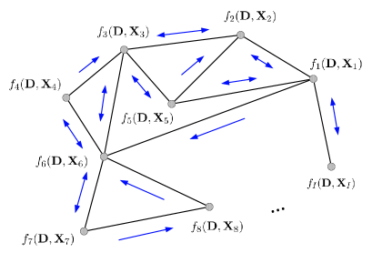
Figure 1: Directed network topology

$$\min_{\mathbf{D},\{\mathbf{X}_{i}\}_{i=1}^{I}} U(\mathbf{D},\mathbf{U})\triangleq\underset{\triangleq F(\mathbf{D},\mathbf{X})}{\underbrace{\sum_{i=1}^{I}f_{i}(\mathbf{D},\mathbf{X}_{i})}}+\sum_{i=1}^{I}g_{i}(\mathbf{X}_{i})+G(\mathbf{D})$$ (P)

$$\mathrm{s.t.} \mathbf{D}\in{\cal D},~{}\mathbf{X}_{i}\in\mathcal{X}_{i},\quad i=1,\ldots,I,$$

where $f_{i}:\mathcal{D}\times\mathcal{X}_{i}\rightarrow\mathbb{R}$ is the fidelity function of agent $i$, which measures the mismatch between the data $\mathbf{S}_{i}$ and the (local) model; this function is assumed to be smooth and biconvex (i.e., convex in $\mathbf{D}$ for fixed $\mathbf{X}_{i}$, and vice versa); $G:\mathcal{D}\rightarrow\mathbb{R}$ and $g_{i}:\mathcal{X}_{i}\rightarrow\mathbb{R}$ are (possibly non-smooth) convex functions, which are generally used to impose extra structure on the solution (e.g., low-rank or sparsity); and $\mathcal{D}\subseteq\mathbb{R}^{M\times K}$ and $\mathcal{X}_{i}\subseteq\mathbb{R}^{K\times n_{i}}$ are some closed convex sets. To avoid scaling ambiguity in the model, $\mathcal{D}$ is assumed to be bounded, without loss of generality. Since all $f_{i}$’s share the common variable $\mathbf{D}$, we call it a shared variable and, by the same token, $\mathbf{X}_{i}$’s are termed private variables. Note that, in this distributed setting, agent $i$ knows only its own functions $f_{i}$ (and $g_{i}$) but not $\sum_{j\neq i}f_{j}$. Hence, agents aim to cooperatively solve Problem P leveraging local communications with their neighbors.

Problem P encompasses several DL-based formulations of practical interest, corresponding to different choices of the fidelity functions, regularizers, and feasible sets; examples include the elastic net (Zou and Hastie, 2005) sparse DL, sparse PCA (Shen and Huang, 2008), non-negative matrix factorization and low-rank approximation (Hastie et al., 2015), supervised DL (Mairal et al., 2008), sparse singular value decomposition (Lee et al., 2010), non-negative sparse coding (Hoyer, 2004), principal component pursuit (Candès et al., 2011), robust non-negative sparse matrix factorization, and discriminative label consistent learning (Jiang et al., 2011). More details on explicit customizations of the general model P can be found in Sec. 2.

Our distributed setting is motivated by several data-intensive applications in several fields, including signal processing and machine learning, and network systems (such as clouds, cluster computers, networks of sensor vehicles, or autonomous robots) wherein the sheer volume and spatial/temporal disparity of scattered data, energy constraints, and/or privacy issues, render centralized processing and storage infeasible or inefficient. Also, time-varying communications arise, for instance, in mobile wireless networks (e.g., ad-hoc networks), wherein nodes are mobile and/or communicate through fading channels. Moreover, since nodes generally transmit at different power and/or communication channels are not symmetric, directed links are a natural assumption.

Our goal is to design a provably convergent decentralized method for Problem P, over time-varying and directed graphs. To the best of our knowledge this is an open problem, as documented next.

1.1 Challenges and related works

The design of distributed algorithms for P faces the following challenges:

1. Problem P is non-convex and non-separable in the optimization variables;

2. Each agent $i$ owns exclusively $\mathbf{S}_{i}$ and thus can only compute its own function $f_{i}$;

3. Each $f_{i}$ depends on a common set of variables$-$the dictionary $\mathbf{D}-$shared among all the agents, as well as the private variables $\mathbf{X}_{i}$. Shared and private variables need to be treated differently. In fact, in several applications, the size of private variables is much larger than that of the shared ones; hence, broadcasting agents’ private variables over the network would result in an unaffordable communication overhead;

4. The gradient of each $f_{i}$ is in general neither bounded nor globally Lipschitz on the feasible region. This represents a challenge in the design of provably convergent distributed algorithms, as boundedness of the gradient is a standard assumption in the analysis of most distributed schemes for nonconvex problems;

5. $G$ and $g_{i}$’s are nonsmooth;

6. The graph is directed, time-varying; no other structure is assumed (such as star or ring topology, etc.), but some long term connectivity properties (cf. Assumption B).

Centralized methods for the solution of Problem P (or some closely related variants) have been extensively studied and prominent examples are (Aharon et al., 2006; Mairal et al., 2010; Razaviyayn et al., 2014b). However, we are not aware of any distributed algorithm that can address challenges i)-vi) (even some subsets of them), as documented next.

Ad-hoc heuristics: Several attempts have been made to extend centralized approaches for DL problems to a distributed setting (undirected, static graphs), under more or less restrictive assumptions; examples include primal methods (Raja and Bajwa, 2013; Chainais and Richard, 2013; Wai et al., 2015) and (primal/)dual-based ones (Chen et al., 2015; Liang et al., 2014; Chouvardas et al., 2015). While these schemes represent good heuristics, their theoretical convergence remains an open question, and numerical results are contradictory. For instance, some schemes are shown not to converge while some others fail to reach asymptotic agreement among the local copies of the dictionary; see, e.g. (Chainais and Richard, 2013).

Recently and independently from our conference work (Daneshmand et al., 2016), Zhao et al. (2016) proposed a distributed primal-dual-based method for a class of dictionary learning problems related, but different from Problem P. Specifically, they considered: quadratic loss functions $f_{i}$, with a quadratic regularization on the dictionary (i.e., $G=0$), and norm ball constraints on the private variables. The network is modeled as a fixed undirected graph. Asymptotic convergence of the scheme to stationary solutions is proved, but no rate analysis is reported. We remark that the scheme in (Zhao et al., 2016), in order to establish convergence, requires some penalty parameters to go to infinity, which makes the method numerically not attractive.

Distributed nonconvex optimization: Since the DL problem P is an instance of non-convex optimization problems, we briefly discuss here the few works in the literature on distributed methods for non-convex optimization (Bianchi and Jakubowicz, 2013; Tatarenko and Touri, 2017; Wai et al., 2017; Di Lorenzo and Scutari, 2016; Sun et al., 2016; Hong et al., 2017; Scutari and Sun, 2019); we group these papers as follows. The schemes in (Bianchi and Jakubowicz, 2013; Tatarenko and Touri, 2017; Wai et al., 2017; Hong et al., 2017), while substantially different, are all applicable to smooth, unconstrained optimization, with (Bianchi and Jakubowicz, 2013; Wai et al., 2017) handling also compact constraints and (Tatarenko and Touri, 2017) implementable on (time-varying) digraphs. The distributed algorithms in (Di Lorenzo and Scutari, 2016; Sun et al., 2016; Scutari and Sun, 2019) can handle objectives with additive nonsmooth convex functions, with (Sun et al., 2016; Scutari and Sun, 2019) applicable to (time-varying) digraphs.

All the above schemes cannot adequately deal with private (i.e., $\mathbf{X}_{i}$’s) and shared variables (i.e., $\mathbf{D}$), which are a key feature of Problem P. Furthermore, convergence therein is proved under the assumption that the gradient of (the smooth part of) the objective function is globally Lipschitz continuous, a property that we do not assume and that is not satisfied in many of the applications we consider. The design of provably convergent distributed algorithms for P remains an open problem, let alone rate guarantees.

1.2 Major contributions

In this paper, we propose the first provably convergent distributed algorithm for the general class of DL problems P, addressing all challenges i)-vi). The proposed approach uses a general convexification-decomposition technique that hinges on recent (centralized) Successive Convex Approximation methods (Scutari et al., 2014; Facchinei et al., 2015). This technique is coupled with a perturbed push-sum consensus scheme preserving the feasibility of the iterates and a tracking mechanism aiming at estimating locally the gradient of $\sum_{i}f_{i}$. Both communication and tracking protocols are implementable on time-varying undirected or directed graphs (B-strongly connected). The scheme is proved to converge to stationary solutions of Problem P, under mild assumptions on the step-size employed by the algorithm; a sublinear convergence rate is also established. On the technical side, we contribute to the literature of distributed algorithms for bi-convex (nonsmooth) constrained optimization by putting forth a new non-trivial convergence analysis that, for the first time, i) avoids the assumption that the gradients $\nabla f_{i}$ are globally Lipschitz; and ii) deals with private and shared optimization variables. Numerical experiments show that the proposed schemes compare favorably with ad-hoc algorithms, proposed for special instances of Problem P.

1.3 Paper Organization

The rest of the paper is organized as follows. The problem and network setting are introduced in Sec. 2, along with some motivating applications. Sec. 3 presents the algorithm and its convergence properties; the proofs of our results are given in the Appendix, Sec. A. Extensive numerical experiments showing the effectiveness of the proposed scheme are discussed in Sec. 5 whereas Sec. 6 draws some conclusions.

1.4 Notation

Throughout the paper we use the following notation. We denote by $\mathbb{N}_{+}$ the set of non-negative integers. Given $x\in\mathbb{R}$, $\lceil x\rceil$ (resp. $\lfloor x\rfloor$) denotes the smallest (resp. the largest) integer greater (resp. smaller) than or equal to $x$. Vectors are denoted by bold lower-case letters (e.g., $\mathbf{x}$) whereas matrices are denoted by bold capital letters (e.g., $\mathbf{A}$). The $k$-th canonical vector is denoted by $\mathbf{e}_{k}$. The inner product between two real matrices, $\mathbf{A}$ and $\mathbf{B}$, is denoted by $\left\langle\mathbf{A},\mathbf{B}\right\rangle\triangleq\mathrm{tr}(\mathbf{A}^{\intercal}\mathbf{B})$, where $\text{tr}(\bullet)$ is the trace operator; $\mathbf{A}\otimes\mathbf{B}$ denotes the Kronecker product. Given the real matrix $\mathbf{A}$, with $ij$-entries denoted by $A_{ij}$, we will use the following matrix norms: the Frobenius norm $||\mathbf{A}||_{F}\triangleq\sqrt{\sum_{i,j}|A_{ij}|^{2}}$; the $L_{1,1}$ norm $||\mathbf{A}||_{1,1}\triangleq\sum_{i,j}|A_{ij}|$; the $L_{2,\infty}$ norm $||\mathbf{A}||_{2,\infty}\triangleq\max_{i}\,\sqrt{\sum_{j}A_{ij}^{2}}$; the $L_{\infty,\infty}$ norm $||\mathbf{A}||_{\infty,\infty}=\max_{i,j}|A_{ij}|$; and the spectral norm $||\mathbf{A}||_{2}\triangleq\sigma_{\mathrm{max}}(\mathbf{A})$, where $\sigma_{\mathrm{max}}(\mathbf{A})$ denotes the maximum singular value of $\mathbf{A}$. The matrix quantities $\nabla_{D}f_{i}(\mathbf{D},\mathbf{X}_{i})$ and $\nabla_{X_{i}}f_{i}(\mathbf{D},\mathbf{X}_{i})$ are the gradients of $f_{i}$ with respect to $\mathbf{D}$ and $\mathbf{X}_{i}$, evaluated at $(\mathbf{D},\mathbf{X}_{i})$, respectively, with the partial derivatives arranged according to the patterns of $\mathbf{D}$ and $\mathbf{X}_{i}$, respectively. The same convention is adopted for subgradients of $g_{i}$ and $G$, that are therefore written as matrices of the same dimensions of $\mathbf{X}_{i}$ and $\mathbf{D}$, respectively. Table 1 summarizes the main notation and symbols used in the paper.

Because of the nonconvexity of Problem P, we aim at computing stationary solutions of P, defined as follows: a tuple $({\mathbf{D}^{\ast}},\mathbf{X}^{\ast})$, with $\mathbf{X}^{\ast}\triangleq[\mathbf{X}_{1}^{\ast},\dots,\mathbf{X}_{I}^{\ast}]$ is a stationarity solution of P if the following holds: $\mathbf{D}^{\ast}\in\mathcal{D}$, $\mathbf{X}_{i}^{\ast}\in\mathcal{X}_{i}$, $i=1,\ldots,I$, and

$$\Big{\langle}\nabla_{D}F({\mathbf{D}^{\ast}},{\mathbf{X}^{\ast}}),\mathbf{D}-\mathbf{D}^{\ast}\Big{\rangle}+G(\mathbf{D})-G(\mathbf{D}^{\ast})\,\geq\,0, \forall\,\mathbf{D}\in{\cal D},$$ (2)

$$\left\langle\nabla_{X_{i}}f_{i}(\mathbf{D}^{\ast},\mathbf{X}_{i}^{\ast}),\mathbf{X}_{i}-{\mathbf{X}}_{i}^{\ast}\right\rangle+g_{i}(\mathbf{X}_{i})-g_{i}(\mathbf{X}_{i}^{\ast})\,\geq\,0, \forall\mathbf{X}_{i}\in\mathcal{X}_{i},\;i=1,\ldots,I.$$

Symbol	Definition	Member of	Reference
$F(\mathbf{D},\mathbf{X})$	$\sum_{i=1}^{I}f_{i}(\mathbf{D},\mathbf{X}_{i})$	$\mathbb{R}^{M\times K}\times\mathbb{R}^{K\times N}\rightarrow\mathbb{R}$	(P)
$U(\mathbf{D},\mathbf{X})$	$F(\mathbf{D},\mathbf{X})+\sum_{i=1}^{I}g_{i}(\mathbf{X}_{i})+G(\mathbf{D})$	$\mathbb{R}^{M\times K}\times\mathbb{R}^{K\times N}\rightarrow\mathbb{R}$	(P)
$\mathbf{S}_{i}$	Local data matrix	$\mathbb{R}^{M\times n_{i}}$
$\mathbf{S}$	$[\mathbf{S}_{1},\mathbf{S}_{2},\ldots,\mathbf{S}_{I}]$	$\mathbb{R}^{M\times N}$
$\mathbf{D}$	Dictionary matrix variable	$\mathcal{D}\subseteq\mathbb{R}^{M\times K}$
$\mathbf{D}_{(i)}$	Local copy of $\mathbf{D}$ of agent $i$	$\mathcal{D}\subseteq\mathbb{R}^{M\times K}$
$\mathbf{D}^{\nu}_{(i)}$	$\mathbf{D}_{(i)}$ at iteration $\nu$	$\mathcal{D}\subseteq\mathbb{R}^{M\times K}$
$\mathbf{D}^{\nu}$	$[\mathbf{D}_{(1)}^{\nu\intercal},\mathbf{D}_{(2)}^{\nu\intercal},\ldots,\mathbf{D}_{(I)}^{\nu\intercal}]^{\intercal}$	$\mathbb{R}^{M\times KI}$	(25)
$\widetilde{\mathbf{D}}_{(i)}^{\nu}$	Solution of subproblem (8)	$\mathcal{D}\subseteq\mathbb{R}^{M\times K}$	(8)
$\overline{\mathbf{D}}^{\nu}$	$(1/I)\sum_{i=1}^{I}\mathbf{D}_{(i)}^{\nu}$	$\mathcal{D}\subseteq\mathbb{R}^{M\times K}$	(25)
$\mathbf{U}^{\nu}_{(i)}$	Local update of dictionary variable	$\mathcal{D}\subseteq\mathbb{R}^{M\times K}$	(10)
$\mathbf{X}_{i}$	Local matrix variable	$\mathcal{X}_{i}\subseteq\mathbb{R}^{K\times n_{i}}$
$\mathbf{X}$	$[\mathbf{X}_{1},\mathbf{X}_{2},\ldots,\mathbf{X}_{I}]$	$\mathcal{X}\subseteq\mathbb{R}^{K\times N}$
$\mathbf{X}_{i}^{\nu}$	$\mathbf{X}_{i}$ at iteration $\nu$	$\mathcal{X}_{i}\subseteq\mathbb{R}^{K\times n_{i}}$
$\mathbf{X}^{\nu}$	$\mathbf{X}$ at iteration $\nu$ : $[\mathbf{X}_{1}^{\nu},\mathbf{X}_{2}^{\nu},\ldots,\mathbf{X}_{I}^{\nu}]$	$\mathcal{X}\subseteq\mathbb{R}^{K\times N}$	(25)
$\boldsymbol{\Theta}^{\nu}_{(i)}$	Gradient-tracking variable	$\mathcal{D}\subseteq\mathbb{R}^{M\times K}$	(13)
$\mathbf{A}^{\nu}$	$(a_{ij}^{\nu})_{i,j=1}^{I}-$ consensus weights at time $\nu$	$\mathbb{R}^{I\times I}$	Assumption F

Table 1: Table of notation

2 Problem Setup and Motivating Examples

In this section, we first discuss the assumptions underlying our model and then provide several examples of possible applications.

2.1 Problem Assumptions

We consider Problem P under the following assumptions.

Assumption A (On Problem P)

• Each $f_{i}:\mathcal{O}\times\mathcal{O}_{i}\rightarrow\mathbb{R}$ is $\mathcal{C}^{2}$, lower bounded, and biconvex, where $\mathcal{O}\supseteq\mathcal{D}$ and $\mathcal{O}_{i}\supseteq\mathcal{X}_{i}$ are convex open sets;

• Given $\mathbf{D}\in\mathcal{D}$, each $\nabla_{X_{i}}f_{i}(\mathbf{D},\bullet)$ is Lipschitz continuous on $\mathcal{X}_{i}$, with Lipschitz constant $L_{\nabla{X_{i}}}(\mathbf{D})$. Furthermore, each $L_{\nabla{X_{i}}}:\mathcal{D}\rightarrow\mathbb{R}$ is continuous;

• $\!\mathcal{D}$ is compact and convex; and each $\mathcal{X}_{i}$ is closed and convex (not necessarily bounded);

• $G:\mathcal{O}\rightarrow\mathbb{R}$ is convex (possibly non-smooth);

• For all $i=1,\ldots,I$, either i) $\mathcal{X}_{i}$ is compact and $g_{i}:\mathcal{O}_{i}\rightarrow\mathbb{R}$ is convex; or ii) $g_{i}$ is $\mu_{i}$-strongly convex.

The above assumptions are quite mild and are satisfied by several problems of practical interest; see Sec. 2.2 for several concrete examples.

Network topology

We study Problem P in the following network setting. Time is slotted and in each time-slot $\nu$ the network of the $I$ agents is modeled as a digraph $\mathcal{G}^{\nu}=(\mathcal{V},\mathcal{E}^{\nu})$, where $\mathcal{V}=\{1,\ldots,I\}$ is the set of agents and $\mathcal{E}^{\nu}$ is the set of edges (communication links); we use $(i,j)\in\mathcal{E}^{\nu}$ to indicate that there is a directed link from node $i$ to node $j$. The in-neighborhood of agent $i\in\mathcal{V}$ at time $\nu$ is defined as $\mathcal{N}_{i}^{\rm in}[\nu]=\{j\in\mathcal{V}|(j,i)\in\mathcal{E}^{\nu}\}\cup\{i\}$ (see Fig. 2) whereas its out-neighborhood is $\mathcal{N}_{i}^{\textrm{out}}\left[\nu\right]=\{j\in\mathcal{V}|\left(i,j\right)\in\mathcal{E}^{\nu}\}\cup\{i\}$. In words, agent $i$ can receive information from its in-neighborhood members, and send information to its out-neighbors. The out-degree of agent $i$ is defined as $d_{i}^{\nu}\triangleq\left|\mathcal{N}_{i}^{\textrm{out}}\left[\nu\right]\right|$, where $\left|\bullet\right|$ denotes the cardinality of a set. If the graph is undirected, the set of in-neighbors and out-neighbors coincide; in such a case we just write $\mathcal{N}_{i}$ to denote the set of neighbors of agent $i$. When the network is static, all the above quantities do not depend on the iteration index $\nu$; hence, we will drop the superscript “$\nu$”. To let information propagate over the network, we assume that the sequence $\{\mathcal{G}^{\nu}\}_{\nu}$ possesses some “long-term” connectivity property, as stated next.

Figure 2: Illustration of in-neighborhood set of agent $i$ at time $\nu$.

Assumption B (B-strong connectivity)

The graph sequence $\{\mathcal{G}^{\nu}\}_{\nu}$ is $B$-strongly connected, i.e., there exists an (arbitrarily large) integer $B>0$ (unknown to the agents) such that the graph with edge set $\cup_{t=kB}^{(k+1)B-1}\mathcal{E}^{t}$ is strongly connected, for all $k\geq 0$.

Notice that this condition is quite mild and widely used in the literature to analyze convergence of distributed algorithms over time-varying networks. Generally speaking, it permits strong connectivity to occur over time windows of length $B$, so that information can propagate from every node to every other node in the network. Assumption B is satisfied in several practical scenarios. For instance, commonly used settings in cloud computing infrastructures are star, ring, tree, hypercube, or n-dimensional mesh (Torus) topologies, which all satisfy Assumption B. It is worth mentioning that the multi-hop network topologies of these structures are migrating towards high-radix mesh and Torus, since they are scalable, low-energy consuming, and much cheaper than other topologies, like fat-tree topologies (Kim, 2008). These type of connected networks are generally time-invariant and undirected, and clearly they satisfy Assumption B.

2.2 Motivating examples

We conclude this section discussing some practical instances of Problem P, all satisfying Assumption A, which show the generality of the proposed model.

Elastic net sparse DL (Tosic and Frossard, 2011; Zou and Hastie, 2005)

Sparse approximation of a signal with an adaptive dictionary is one of the most studied DL problems (Tosic and Frossard, 2011). When an elastic net sparsity-inducing regularizer is used (Zou and Hastie, 2005), the problem can be written as

$$\min_{\mathbf{D},\{\mathbf{X}_{i}\}_{i=1}^{I}} \sum_{i=1}^{I}~{}\left\{\frac{1}{2}\,\left\lVert\mathbf{S}_{i}-\mathbf{D}\mathbf{X}_{i}\right\rVert_{F}^{2}+\lambda\left\lVert\mathbf{X}_{i}\right\rVert_{1,1}+\frac{\mu}{2}\left\lVert\mathbf{X}_{i}\right\rVert_{F}^{2}\right\}$$ (3)

$$\mathrm{s.t.} \mathbf{D}\in{\cal D},~{}\mathbf{X}_{i}\in\mathbb{R}^{K\times n_{i}},\quad i=1,2,\ldots,I,$$

where $\mathcal{D}\triangleq\{\mathbf{D}\,:\,||\mathbf{D}\mathbf{e}_{k}||_{2}\leq\alpha,\,k=1,2,\ldots,K\}$, and $\alpha,\,\lambda,\,\mu>0$ are the tuning parameters. Problem (3) is an instance of P, with $f_{i}(\mathbf{D},\mathbf{X}_{i})=({1}/{2})\cdot\left\lVert\mathbf{S}_{i}-\mathbf{D}\mathbf{X}_{i}\right\rVert_{F}^{2}$, $g_{i}(\mathbf{X}_{i})=\lambda\left\lVert\mathbf{X}_{i}\right\rVert_{1,1}+\frac{\mu}{2}\left\lVert\mathbf{X}_{i}\right\rVert_{F}^{2}$, $G(\mathbf{D})=0$, and $\mathcal{X}_{i}=\mathbb{R}^{K\times n_{i}}$. It is not difficult to check that (3) satisfies Assumption A, and the Lipschitz constant in A2 is given by $L_{\nabla X_{i}}(\mathbf{D})=(\sigma_{\mathrm{max}}(\mathbf{D}))^{2}$.

Supervised DL (Mairal et al., 2008)

Consider a classification problem with training set $\{\mathbf{s}_{n},y_{n}\}_{n=1}^{N}$, where $\mathbf{s}_{n}$ is the feature vector with associated binary label $y_{n}$. The discriminative DL problem aims at simultaneously learning a dictionary $\mathbf{D}^{(1)}\in\mathbb{R}^{M\times K}$ such that $\mathbf{s}_{n}=\mathbf{D}^{(1)}\mathbf{x}_{n}$, for some sparse $\mathbf{x}_{n}\in\mathbb{R}^{K}$, and finding a bilinear classifier $\zeta_{n}(\mathbf{D}^{(2)},\mathbf{x}_{n},\mathbf{s}_{n})\triangleq\mathbf{s}_{n}^{\intercal}\,\mathbf{D}^{(2)}\,\mathbf{x}_{n}$ that best separates the coded data with distinct labels (Mairal et al., 2008). Assume that each agent $i$ owns $\{\left(\mathbf{s}_{n},y_{n}\right)\,:\,n\in\mathcal{S}_{i}\}$, with $\{\mathcal{S}_{i}\}_{i=1}^{I}$ being a partition of $\{1,\ldots,N\}$, then the discriminative DL reads

$$\min_{\begin{subarray}{c}\mathbf{D}^{(1)},\mathbf{D}^{(2)}\\ \{\mathbf{x}_{n}\}_{n=1}^{N}\end{subarray}} \sum_{i=1}^{I}\sum_{n\in\mathcal{S}_{i}}\left[\ell\left(y_{n}\zeta_{n}\left(\mathbf{D}^{(2)},\mathbf{x}_{n},\mathbf{s}_{n}\right)\right)+\frac{1}{2}\left\lVert\mathbf{s}_{n}-\mathbf{D}^{(1)}\mathbf{x}_{n}\right\rVert_{2}^{2}+g_{n}(\mathbf{x}_{n})\right]$$ (4)

$$\mathrm{s.t.} \mathbf{D}^{(1)}\in{\cal D}^{(1)},~{}\mathbf{D}^{(2)}\in\mathcal{D}^{(2)},\ {\mathbf{x}_{n}\in\mathbb{R}^{K}},\quad n=1,2,\ldots,N,$$

where $\ell(x)\triangleq\log(1+e^{-x})$ is the logistic loss function; and $g_{n}\left(\mathbf{x}_{n}\right)\triangleq\lambda\left\lVert\mathbf{x}_{n}\right\rVert_{1}+({\mu}/{2})\cdot\left\lVert\mathbf{x}_{n}\right\rVert_{2}^{2}$ is the elastic net regularizer. The dictionary $\mathbf{D}^{(1)}$ and classifier parameter $\mathbf{D}^{(2)}$ are constrained to belong to the convex compact sets $\mathcal{D}^{(1)}$ and $\mathcal{D}^{(2)}$, respectively. Problem (4) is an instance of Problem P, with $\mathbf{D}\triangleq\left[\mathbf{D}^{(1)},\mathbf{D}^{(2)}\right]$, $\mathbf{S}_{i}\triangleq\left[\mathbf{s}_{n}\right]_{n\in\mathcal{S}_{i}}$ and $\mathbf{X}_{i}\triangleq\left[\mathbf{x}_{n}\right]_{n\in\mathcal{S}_{i}}$. Note that Assumption A is satisfied, and the Lipschitz constant in A2 is given by $L_{\nabla X_{i}}(\mathbf{D})=({1}/{4})\cdot\|y_{i}\cdot\mathbf{s}_{i}^{\intercal}\,\mathbf{D}^{(2)}\|_{2}^{2}+(\sigma_{\mathrm{max}}(\mathbf{D}^{(1)}))^{2}.$

DL for low-rank plus sparse representation (Bouwmans et al., 2017)

The low-rank plus sparse decomposition problems cover many applications in signal processing and machine learning (Bouwmans et al., 2017), including matrix completion, image denoising, deblurring, superresolution, and Principal Component Pursuit (PCP) (Candès et al., 2011). Consider the bi-linear model $\mathbf{S}\approx\mathbf{L}+\mathbf{H}\mathbf{Q}\mathbf{U}$: the data matrix $\mathbf{S}$ is decomposed as the superposition of a low-rank matrix $\mathbf{L}$ (capturing the correlations among data) and $\mathbf{H}\mathbf{Q}\mathbf{U}$, where $\mathbf{Q}\in\mathbb{R}^{M\times\tilde{K}}$ is an over-complete dictionary (capturing the representative modes of the data), $\mathbf{U}\in\mathbb{R}^{\tilde{K}\times N}$ is a sparse matrix (representing the data parsimoniously), and $\mathbf{H}$ is a given degradation matrix, which accounts for tasks such as denoising, superresolution, and deblurring. To enforce $\mathbf{L}$ to be low-rank, we employ the nuclear norm $\left\lVert\mathbf{L}\right\rVert_{*}$ regularizer, which can be equivalently rewritten as $\left\lVert\mathbf{L}\right\rVert_{*}=\inf\{\frac{1}{2}\left\lVert\mathbf{P}\right\rVert_{F}^{2}+\frac{1}{2}\left\lVert\mathbf{V}\right\rVert_{F}^{2}\,:\,\mathbf{L}=\mathbf{P}\mathbf{V}\}$, where $\mathbf{P}\in\mathbb{R}^{M\times L}$, $\mathbf{V}\in\mathbb{R}^{L\times N}$, and $L\ll\min(M,N)$ (Srebro and Shraibman, 2005; Recht et al., 2010). Partitioning $\mathbf{V}$ and $\mathbf{U}$ according to $\mathbf{S}$, i.e., $\mathbf{S}_{i}=\mathbf{P}\mathbf{V}_{i}+\mathbf{H}\mathbf{Q}\mathbf{U}_{i}$, the problem reads

$$\min_{\begin{subarray}{c}\mathbf{P},\mathbf{Q},(\mathbf{V}_{i},\mathbf{U}_{i})_{i=1}^{I}\end{subarray}} \sum_{i=1}^{I}~{}\Bigg{[}\frac{1}{2}~{}\Big{\|}\mathbf{S}_{i}-\left[\mathbf{P}~{}\mathbf{H}\mathbf{Q}\right]{\begin{bmatrix}\mathbf{V}_{i}\\ \mathbf{U}_{i}\end{bmatrix}}\Big{\|}_{F}^{2}$$ (5)

$$\qquad\qquad\qquad\quad+\frac{\zeta}{2I}\left(\left\lVert\mathbf{P}\right\rVert_{F}^{2}+I\cdot\left\lVert\mathbf{V}_{i}\right\rVert_{F}^{2}\right)+\lambda\left\lVert\mathbf{X}_{i}\right\rVert_{1,1}+\frac{\mu}{2}\left\lVert\mathbf{X}_{i}\right\rVert_{F}^{2}\Bigg{]}$$

$$\mathrm{s.t.} \mathbf{D}\in{\cal D},\quad{\mathbf{X}_{i}\in\mathbb{R}^{(L+\tilde{K})\times n_{i}},\quad i=1,2,\ldots,I,}$$

where $\mathcal{D}$ is some compact set; $\zeta>0$ is a constant used to promote the low-rank structure on $\mathbf{L}$ while sparsity on $\mathbf{X}$ is enforced by the elastic net regularization, with constants $\lambda,\,\mu>0$. Problem (5) is clearly an instance of Problem P wherein $f_{i}$ is the quadratic loss, and $[\mathbf{P},\mathbf{Q}]$ and $[\mathbf{V}_{i}^{\intercal},\mathbf{U}_{i}^{\intercal}]^{\intercal}$ are the shared and private variables ($K=L+\tilde{K}$), respectively. Assumption A is satisfied, and the Lipschitz constant in A2 is given by $L_{\nabla X_{i}}(\mathbf{D})=(\sigma_{\mathrm{max}}(\mathbf{\mathbf{P}\mathbf{H}\mathbf{Q}}))^{2}$.

A variant of this problem, which still is a particular case of Problem (5), is obtained by replacing the quadratic loss function with the smoothed Huber function to achieve robustness against outliers (Aravkin et al., 2014).

Sparse SVD/PCA (Lee et al., 2010; Udell et al., 2016; Mairal et al., 2010)

Computing the SVD of a set of data with sparse singular vectors (Sparse SVD) is the foundation of many applications in multivariate analysis, e.g., biclustering (Lee et al., 2010). As proposed in (Mairal et al., 2010), Problem P can be used to accomplish this task by imposing sparsity on the factors $\mathbf{D}$ and $\mathbf{X}$ of $\mathbf{S}$. More specifically, we have

$$\min_{\mathbf{D},(\mathbf{X}_{i})_{i=1}^{I}} \sum_{i=1}^{I}~{}\left\{\frac{1}{2}~{}\left\lVert\mathbf{S}_{i}-\mathbf{D}\mathbf{X}_{i}\right\rVert_{F}^{2}+\lambda_{X}\left\lVert\mathbf{X}_{i}\right\rVert_{1,1}+\frac{\mu_{X}}{2}\left\lVert\mathbf{X}_{i}\right\rVert_{F}^{2}\right\}+\lambda_{D}\left\lVert\mathbf{D}\right\rVert_{1,1}+\frac{\mu_{D}}{2}\left\lVert\mathbf{D}\right\rVert_{F}^{2}$$ (6)

$$\mathrm{s.t.} \mathbf{D}\in{\cal D}\triangleq\{\mathbf{D}\in\mathbb{R}^{M\times K}\,:\,||\mathbf{D}||_{2,\infty}\leq\alpha\},\quad{\mathbf{X}_{i}\in\mathbb{R}^{K\times n_{i}},\quad i=1,2,\ldots,I,}$$

where $\lambda_{D},\,\lambda_{X},\,\mu_{D},\,\mu_{X},\,\alpha>0$ are given constants. Problem (6) is an instance of P, with $f_{i}(\mathbf{D},\mathbf{X}_{i})=({1}/{2})\cdot||\mathbf{S}_{i}-\mathbf{DX}_{i}||^{2}_{F}$; $G(\mathbf{D})=\lambda_{D}\,||\mathbf{D}||_{1,1}+({\mu_{D}}/{2})\cdot||\mathbf{D}||_{F}^{2}$, and $g_{i}(\mathbf{X}_{i})=\lambda_{X}\,||\mathbf{X}_{i}||_{1,1}+({\mu_{X}}/{2})\cdot\,||\mathbf{X}_{i}||^{2}_{F}$. Note that orthonormality of factors are relaxed for sake of simplicity. A related formulation, termed Sparse PCA, has also been used in (Udell et al., 2016). It is not difficult to show that Assumption A is satisfied, and the Lipschitz constant in A2 is given by $L_{\nabla X_{i}}(\mathbf{D})=(\sigma_{\mathrm{max}}(\mathbf{D}))^{2}$.

Non-negative Sparse Coding (NNSC) (Hoyer, 2004)

Non-negative Matrix Factorization (NMF) was primarily proposed by (Lee and Seung, 1999) as a better alternative to the classic SVD in learning localized features of image datasets, such as face images. The formulation enforces non-negativity of the entries of $\mathbf{D}$ and $\mathbf{X}$. This has been shown to empirically lead to sparse solutions; however no explicit control on sparsity is employed in the model. To overcome this shortcoming, (Hoyer, 2004) proposed a non-negative sparse coding (NNSC) formulation which extends NMF by adding a sparsity-inducing penalty function of $\mathbf{X}$. The problem reads

$$\min_{\mathbf{D},(\mathbf{X}_{i})_{i=1}^{I}} \sum_{i=1}^{I}~{}\left\{\frac{1}{2}\,\left\lVert\mathbf{S}_{i}-\mathbf{D}\mathbf{X}_{i}\right\rVert_{F}^{2}+\lambda\,\left\lVert\mathbf{X}_{i}\right\rVert_{1,1}+\frac{\mu}{2}\,\left\lVert\mathbf{X}_{i}\right\rVert_{F}^{2}\right\}$$ (7)

$$\mathrm{s.t.} \mathbf{D}\in{\cal D}\triangleq{\{\mathbf{D}\in\mathbb{R}_{+}^{M\times K}~{}|~{}||\mathbf{D}||_{2,\infty}\leq\alpha\}},~{}\mathbf{X}_{i}\in\mathbb{R}^{K\times n_{i}}_{+},\quad i=1,2,\ldots,I,$$

for some $\lambda,\,\mu,\,\alpha>0$. Problem (7) is another instance of P, with $f_{i}(\mathbf{D},\mathbf{X}_{i})=({1}/{2})\cdot||\mathbf{S}_{i}-\mathbf{D}\mathbf{X}_{i}||_{F}^{2}$, $g_{i}(\mathbf{X}_{i})=\lambda\left\lVert\mathbf{X}_{i}\right\rVert_{1,1}+({\mu}/{2})\cdot\left\lVert\mathbf{X}_{i}\right\rVert_{F}^{2}$, $G(\mathbf{D})=0$, $\mathcal{D}=\{\mathbf{D}\in\mathbb{R}_{+}^{M\times K}~{}|~{}||\mathbf{D}||_{2,\infty}\leq\alpha\}$, and $\mathcal{X}_{i}=\mathbb{R}_{+}^{K\times n_{i}}$. Assumption A is satisfied, and the Lipschitz constant in A2 is given by $L_{\nabla X_{i}}(\mathbf{D})=(\sigma_{\mathrm{max}}(\mathbf{D}))^{2}$.

3 Algorithmic Design

We introduce now our algorithmic framework. To shed light on the core idea behind the proposed scheme, we begin introducing an informal and constructive description of the algorithm, followed by its formal description along with its convergence properties.

Each agent $i$ controls its private variable $\mathbf{X}_{i}$ and maintains a local copy of the shared variables $\mathbf{D}$, denoted by $\mathbf{D}_{(i)}$, along with an auxiliary variable $\boldsymbol{\Theta}_{(i)}$; we anticipate that $\boldsymbol{\Theta}_{(i)}$ aims at locally estimating the gradient sum $\sum_{j}\nabla_{D}f_{j}(\mathbf{D}_{(i)},\mathbf{X}_{j})$, an information that is not available at agent $i$’s side. The value of these variables at iteration $\nu$ is denoted by $\mathbf{X}_{i}^{\nu}$, $\mathbf{D}_{(i)}^{\nu}$, and $\boldsymbol{\Theta}_{(i)}^{\nu}$, respectively. Roughly speaking, the update of these variables is designed so that asymptotically i) all the $\mathbf{D}_{(i)}$ will be consensual, i.e., $\mathbf{D}_{(i)}=\mathbf{D}_{(j)}$, $\forall i\neq j$; and ii) the tuples $(\mathbf{D}_{(i)},(\mathbf{X}_{j})_{j=1}^{I})$ will be a stationary solutions of Problem P. This is accomplished throughout the following two steps, which are performed iteratively and in parallel across the agents.

Step 1: Local Optimization

The nonconvexity of $f_{i}$ together with the lack of knowledge of $\sum_{j\neq i}f_{j}$ in $F$ prevents agent $i$ to solve directly Problem P with respect to $(\mathbf{D}_{(i)},\mathbf{X}_{i})$. Since $f_{i}$ is bi-convex in $(\mathbf{D}_{(i)},\mathbf{X}_{i})$, a natural approach is then to update $\mathbf{D}_{(i)}$ and $\mathbf{X}_{i}$ in an alternating fashion by solving a local approximation of P. Specifically, at iteration $\nu$, given the iterates $\mathbf{X}_{i}^{\nu}$, $\mathbf{D}_{(i)}^{\nu}$, and $\boldsymbol{\Theta}_{(i)}^{\nu}$, agent $i$ fixes $\mathbf{X}_{i}=\mathbf{X}_{i}^{\nu}$ and solves the following strongly convex problem in $\mathbf{D}_{(i)}$ :

$$\widetilde{\mathbf{D}}_{(i)}^{\nu}\!\triangleq\underset{\mathbf{D}_{(i)}\in\mathcal{D}}{\text{argmin}}~{}\tilde{f}_{i}\big{(}\mathbf{D}_{(i)};\mathbf{D}_{(i)}^{\nu},\mathbf{X}_{i}^{\nu}\big{)}+\left\langle I\cdot{\boldsymbol{\Theta}}_{(i)}^{\nu}-\nabla_{D}f_{i}(\mathbf{D}^{\nu}_{(i)},\mathbf{X}^{\nu}_{i}),\mathbf{D}_{(i)}-\mathbf{D}_{(i)}^{\nu}\right\rangle+G\left(\mathbf{D}_{(i)}\right),$$ (8)

where $\tilde{f}_{i}(\bullet;\mathbf{D}_{(i)}^{\nu},\mathbf{X}_{i}^{\nu})$ is a suitably chosen strongly convex approximation of $f_{i}(\bullet,\mathbf{X}_{i}^{\nu})$ at $(\mathbf{D}_{(i)}^{\nu},\mathbf{X}_{i}^{\nu})$ (cf. Assumption C, Sec. 3.1); and ${\boldsymbol{\Theta}}_{(i)}^{\nu}$, as anticipated, is used to track the gradient of $F$, with $\lim_{\nu\to\infty}\|I\cdot{\boldsymbol{\Theta}}_{(i)}^{\nu}-\sum_{j=1}^{I}\nabla_{D}f_{j}(\mathbf{D}_{(i)}^{\nu},\mathbf{X}_{j}^{\nu})\|=0$; which would lead to

$$\lim_{\nu\to\infty}\left\|\left(I\cdot{\boldsymbol{\Theta}}_{(i)}^{\nu}-\nabla_{D}f_{i}(\mathbf{D}^{\nu}_{(i)},\mathbf{X}^{\nu}_{i})\right)-\sum_{j\neq i}\nabla_{D}f_{j}(\mathbf{D}_{(i)}^{\nu},\mathbf{X}_{j}^{\nu})\right\|=0.$$ (9)

This sheds light on the role of the linear term in (8): it can be regarded as a proxy of the sum-gradient $\sum_{j\neq i}\nabla_{D}f_{j}(\mathbf{D}_{(i)}^{\nu},\mathbf{X}_{j}^{\nu})$, which is not available at agent $i$’s side. In Step 2 below we show how to update ${\boldsymbol{\Theta}}_{(i)}^{\nu}$ using only local information, so that (9) holds.

Given $\widetilde{\mathbf{D}}_{(i)}^{\nu}$, a step-size is employed in the update of $\mathbf{D}_{(i)}$, generating the iterate $\mathbf{U}_{(i)}^{\nu}$:

$$\mathbf{U}_{(i)}^{\nu}=\mathbf{D}_{(i)}^{\nu}+\gamma^{\nu}(\widetilde{\mathbf{D}}_{(i)}^{\nu}-\mathbf{D}_{(i)}^{\nu}),$$ (10)

where $\gamma^{\nu}$ is the step-size, to be properly chosen (see Assumption E, Sec. 3.1).

Let us now consider the update of the private variables $\mathbf{X}_{i}$. Fixing $\mathbf{D}_{(i)}=\mathbf{U}_{(i)}^{\nu}$, agent $i$ computes the new update $\mathbf{X}_{i}^{\nu+1}$ by solving the following strongly convex optimization problem:

$$\mathbf{X}_{i}^{\nu+1}\triangleq\underset{\mathbf{X}_{i}\in\mathcal{X}_{i}}{\text{argmin}}\quad\tilde{h}_{i}(\mathbf{X}_{i};\mathbf{U}_{(i)}^{\nu},\mathbf{X}_{i}^{\nu})+g_{i}(\mathbf{X}_{i}),$$ (11)

where $\tilde{h}_{i}(\bullet;\mathbf{U}_{(i)}^{\nu},\mathbf{X}_{i}^{\nu})$ is a strongly convex function of $\mathbf{X}_{i}$, approximating $f_{i}(\mathbf{U}_{(i)}^{\nu},\bullet)$ at $(\mathbf{U}_{(i)}^{\nu},\mathbf{X}_{i}^{\nu})$; see Assumption C (cf. Sec. 3.1) for specific instances of $\tilde{h}_{i}$.

Step 2: Local Communications

Let us design now a local communication mechanism ensuring asymptotic consensus over the local copies $\mathbf{D}_{(i)}$’s and property (9). To do so, we build on the (perturbed) push-sum protocol proposed in (Sun et al., 2016) (see also Kempe et al. (2003)). Specifically, an extra scalar variable $\phi_{i}$ is introduced at each agent’s side to deal with the directed nature of the graph; given $\phi_{i}^{\nu}$ and $\mathbf{U}_{(j)}^{\nu}$ from its in-neighbors $j\in\mathcal{N}_{i}$, each agent $i$ updates its own local estimate $\mathbf{D}_{(i)}^{\nu}$ and $\phi_{i}^{\nu}$ according to:

$${\phi^{\nu+1}_{i}=\sum_{j\in\mathcal{N}^{\rm in}_{i}[\nu]}a_{ij}^{\nu}\,\phi^{\nu}_{j}\quad\text{and}\quad\mathbf{D}_{(i)}^{\nu+1}=\frac{1}{\phi_{i}^{\nu+1}}\sum_{j\in\mathcal{N}^{\rm in}_{i}[\nu]}a^{\nu}_{ij}\,\phi_{j}^{\nu}\mathbf{U}_{(j)}^{\nu}.}$$ (12)

where $a_{ij}^{\nu}$’s are some weights (to be properly chosen, see Assumption F, Sec. 3.1); and $\phi_{i}^{0}=1$, for all $i=1,\ldots,I$.

Note that the updates in (12) can be implemented locally: all agents only need to (i) send their local variable $\mathbf{U}_{(j)}^{\nu}$ and the scalar weight $a_{ij}^{\nu}\,\phi_{j}^{\nu}$ to their neighbors; and (ii) collect locally the information coming from the neighbors.

To update the $\boldsymbol{\Theta}^{\nu}_{(i)}$ variables we leverage the gradient tracking mechanism first introduced in (Di Lorenzo and Scutari, 2016), coupled with the push-sum consensus scheme (Sun et al., 2016), resulting in the following perturbed push-sum scheme:

$$\boldsymbol{\Theta}^{\nu+1}_{(i)}=\frac{1}{\phi_{i}^{\nu+1}}\sum_{j\in\mathcal{N}_{i}^{\rm in}[\nu]}a_{ij}^{\nu}\phi_{j}^{\nu}\boldsymbol{{\Theta}}_{(j)}^{\nu}+\frac{1}{\phi^{\nu+1}_{i}}\left(\nabla_{D}f_{i}(\mathbf{D}_{(i)}^{\nu+1},\mathbf{X}_{i}^{\nu+1})-\nabla_{D}f_{i}(\mathbf{D}_{(i)}^{\nu},\mathbf{X}_{i}^{\nu})\right),$$ (13)

with $\boldsymbol{{\Theta}}_{(i)}^{0}\triangleq\nabla_{D}f_{i}(\mathbf{D}_{(i)}^{0},\mathbf{X}_{i}^{0})$, for all $i=1,\ldots,I$. The update (13) follows similar logic as that of $\mathbf{D}_{(i)}^{\nu}$ in (12), with the difference that (13) contains a perturbation [the second term in the RHS of (13)], which employs $\boldsymbol{{\Theta}}_{(i)}^{\nu}$ and ensures the desired tracking properties (otherwise $\boldsymbol{{\Theta}}_{(i)}^{\nu}$ would converge to the average of their initial values). Note that (13) can be performed locally by agent $i$, following the same procedure as described for (12).

Combining the above steps, we can now formally introduce the proposed distributed algorithm for the DL problems P, as described in Algorithm 1, and termed D⁴L (Decentralized Dictionary Learning over Dynamic Digraphs) Algorithm.

$\textbf{Initialization}:$ set $\nu=0$ and $\phi^{0}_{i}=1,~{}\mathbf{D}_{(i)}^{0}\in\mathcal{D},~{}\mathbf{X}_{i}^{0}\in\mathcal{X}_{i}$, $\boldsymbol{{\Theta}}_{(i)}^{0}=\nabla_{D}f_{i}(\mathbf{D}^{0}_{(i)},\mathbf{X}^{0}_{i}),$
                       for all $i=1,2,\ldots,I$.
S1. If $(\mathbf{D}_{(i)}^{\nu},\mathbf{X}_{i}^{\nu})$ satisfies a suitable stopping criterion: STOP;
S2. Local Optimization: Each agent $i$ computes:

1. $\widetilde{\mathbf{D}}_{(i)}^{\nu}$ and $\mathbf{U}_{(i)}^{\nu}$ according to (8) and (10);

2. $\mathbf{X}_{i}^{\nu+1}$ according to (11);

S3. Local Communications: Each agent $i$ collects data from its current neighbors and updates:

1. $\phi^{\nu+1}_{i}$ and $\mathbf{D}_{(i)}^{\nu+1}$ according to (12);

2. $\boldsymbol{{\Theta}}^{\nu+1}_{(i)}$ according to (13);

S4. Set $\nu+1\to\nu$, and go to S1.

Algorithm 1 : Decentralized Dictionary Learning over Dynamic Digraphs (D⁴L)

3.1 Algorithmic Assumptions

Before stating the main convergence result for the D⁴L Algorithm, we discuss the main assumptions governing the choices of the free parameters of the algorithm, namely: the surrogate functions $\tilde{f}_{i}$ and $\tilde{h}_{i}$, the step-size $\gamma^{\nu}$, and the consensus weights $(a_{ij}^{\nu})_{i,j=1}^{I}$.

3.1.1 On the choice of $\tilde{f}_{i}$ and $\tilde{h}_{i}$.

The surrogate functions are chosen to satisfy the following assumption.

Assumption C (On $\tilde{f}_{i}$ and $\tilde{h}_{i}$)

Given $\mathbf{D}_{(i)}^{\nu}$ and $\mathbf{X}_{i}^{\nu}$, $\tilde{f}_{i}(\bullet;\mathbf{D}_{(i)}^{\nu},\mathbf{X}_{i}^{\nu})$ in (8) is either

$$\tilde{f}_{i}(\mathbf{D}_{(i)};\mathbf{D}_{(i)}^{\nu},\mathbf{X}_{i}^{\nu})=f_{i}(\mathbf{D}_{(i)},\mathbf{X}_{i}^{\nu})+\frac{\tau_{D,i}^{\nu}}{2}\,||\mathbf{D}_{(i)}-\mathbf{D}_{(i)}^{\nu}||_{F}^{2},$$ (14)

or

$$\tilde{f}_{i}(\mathbf{D}_{(i)};\mathbf{D}_{(i)}^{\nu},\mathbf{X}_{i}^{\nu})=\left\langle\nabla_{D}f_{i}(\mathbf{D}^{\nu}_{(i)},\mathbf{X}_{i}^{\nu}),\mathbf{D}_{(i)}-\mathbf{D}_{(i)}^{\nu}\right\rangle+\frac{\tau_{D,i}^{\nu}}{2}\,\big{\|}\mathbf{D}_{(i)}-\mathbf{D}_{(i)}^{\nu}\big{\|}_{F}^{2},\vspace{-0.1cm}$$ (15)

where $\tau_{D,i}^{\nu}$ is a positive scalar satisfying Assumption D.

Given $\mathbf{U}_{(i)}^{\nu}$ and $\mathbf{X}_{i}^{\nu}$, $\tilde{h}_{i}(\bullet;\mathbf{U}_{(i)}^{\nu},\mathbf{X}_{i}^{\nu})$ in (11) is either

$$\tilde{h}_{i}(\mathbf{X}_{i};\mathbf{U}_{(i)}^{\nu},\mathbf{X}_{i}^{\nu})\triangleq f_{i}(\mathbf{U}_{(i)}^{\nu},\mathbf{X}_{i})+\frac{\tau_{X,i}^{\nu}}{2}\left\lVert\mathbf{X}_{i}-\mathbf{X}_{i}^{\nu}\right\rVert_{F}^{2},$$ (16)

or

$$\tilde{h}_{i}(\mathbf{X}_{i};\mathbf{U}_{(i)}^{\nu},\mathbf{X}_{i}^{\nu})=\left\langle\nabla_{X_{i}}f_{i}(\mathbf{U}_{(i)}^{\nu},\mathbf{X}_{i}^{\nu}),\mathbf{X}_{i}-\mathbf{X}_{i}^{\nu}\right\rangle+\frac{\tau_{X,i}^{\nu}}{2}\big{\|}\mathbf{X}_{i}-\mathbf{X}_{i}^{\nu}\big{\|}_{F}^{2},$$ (17)

where $\tau_{X,i}^{\nu}$ is a positive scalar satisfying Assumption D.

Assumption D (On $\tau_{X,i}^{\nu}$ and $\tau_{D,i}^{\nu}$)

The parameters $(\tau_{X,i}^{\nu})_{i=1}^{I}$ and $(\tau_{D,i}^{\nu})_{i=1}^{I}$ are chosen such that

(D1)

$\{\tau^{\nu}_{D,i}\}_{\nu}$ and $\{\tau^{\nu}_{X,i}\}_{\nu}$ satisfy

$$0<\inf_{\nu}\tau^{\nu}_{D,i}\leq\sup_{\nu}\tau^{\nu}_{D,i}<+\infty,$$ (18)

and

$$\sup_{\nu}\tau^{\nu}_{X,i}<+\infty,\vskip 6.0pt plus 2.0pt minus 2.0pt$$

$$\tau^{\nu}_{X,i}\geq\frac{1}{2}L_{\nabla{X_{i}}}(\mathbf{U}_{(i)}^{\nu})+\epsilon,\quad\forall\nu\geq 1,$$ (19)

for all $i=1,2,\ldots,I$, where $\epsilon>0$ is an arbitrarily small constant, and $L_{\nabla{X_{i}}}$ is defined in Assumption A2.

(D2)

Stronger convergence results [cf. Theorem  2] can be obtained if, under Assumption A5(ii), the sequences $\{\tau^{\nu}_{D,i}\}_{\nu}$ and $\{\tau^{\nu}_{X,i}\}_{\nu}$, in addition to D1, also satisfy

$$\sum_{t=0}^{\infty}\left|\tau^{t+1}_{D,i}-\tau^{t}_{D,i}\right|<\infty,$$ (20)

and

$$\limsup_{\nu}\left|\tau^{\nu}_{X,i}-\tau^{\nu-1}_{X,i}\right|<\mu,$$ (21)

where $\mu\triangleq\min_{i}\mu_{i}$ and $\mu_{i}$ is the strongly convexity constant of $f_{i}$.

Discussion. Several comments are in order.

$\bullet$ On the choice of $\tilde{f}_{i}$ and $\tilde{h}_{i}$. Since $f_{i}$ (resp. $h_{i}$) is convex in $\mathbf{D}_{(i)}$ (resp. $\mathbf{X}_{i}$), (14) [resp. (16)] is a natural choice for the surrogate $\tilde{f}_{i}$ (resp. $\tilde{h}_{i}$): the structure of $f_{i}$ (resp. $h_{i}$) is preserved while a quadratic term is added to make the overall surrogate strongly convex. The non-smooth strongly convex subproblems (8) and (11) resulting from (14) and (16) can be solved using standard solvers, e.g., projected subgradient methods. When dealing with large-scale instances, effective methods are also (Facchinei et al., 2015; Daneshmand et al., 2015).

The alternative surrogates $\tilde{f}_{i}$ and $\tilde{h}_{i}$ as given in (15) and (17), respectively, are based on the the linearization of the original $f_{i}$ and $h_{i}$. This option is motivated by the fact that, for specific instances of $f_{i}$ and $h_{i}$, (15) and (17) lead to subproblems (8) and (11) whose solution can be computed in closed form. For instance, consider the elastic net sparse DL problem (3) in Sec. 2.2, where $f_{i}(\mathbf{D},\mathbf{X}_{i})=\frac{1}{2}||\mathbf{S}_{i}-\mathbf{D}\mathbf{X}_{i}||_{F}^{2}$; $G(\mathbf{D})=0$; and $g_{i}(\mathbf{X}_{i})=\lambda\,||\mathbf{X}_{i}||_{1}+\frac{\mu}{2}\,||\mathbf{X}_{i}||^{2}_{F}$, with $\lambda,\mu>0$. By using (15), the resulting subproblem (8) admits the following closed form solution:

$$\widetilde{\mathbf{D}}_{(i)}^{\nu}=P_{\mathcal{D}}\left[\mathbf{D}_{(i)}^{\nu}-\frac{I}{\tau_{D,i}^{\nu}}\boldsymbol{\Theta}_{(i)}^{\nu}\right].$$ (22)

Referring to the sparse coding subproblem (11), if $\tilde{h}_{i}$ is chosen according to (16), computing the update $\mathbf{X}_{i}^{\nu+1}$ results in solving a LASSO problem. If instead one uses the surrogate in (17), the solution of (11) can be computed in closed form as

$$\mathbf{X}_{i}^{\nu+1}=\frac{\tau^{\nu}_{X,i}}{\mu+\tau^{\nu}_{X,i}}\mathcal{T}_{\frac{\lambda}{\tau^{\nu}_{X,i}}}\left(\mathbf{X}^{\nu}_{i}-\frac{1}{\tau^{\nu}_{X,i}}\nabla_{X_{i}}f_{i}(\mathbf{U}_{(i)}^{\nu},\mathbf{X}_{i}^{\nu})\right),$$ (23)

where $\mathcal{T}$ is the soft-thresholding operator $\mathcal{T}_{\theta}(x)\triangleq\max(|x|-\theta,0)\cdot\text{sign}(x)$ [with $\text{sign}(\cdot)$ denoting the sign function], applied to the matrix argument component-wise.

$\bullet$ On the choice of $\tau_{X,i}^{\nu}$ and $\tau_{D,i}^{\nu}$. These coefficients must satisfy Assumption D. Roughly speaking, D1 ensures that $(\tau_{X,i}^{\nu})_{i=1}^{I}$ and $(\tau_{D,i}^{\nu})_{i=1}^{I}$ are bounded (both from below and above) while D2 guarantees that these parameters are asymptotically “stable”. A trivial choice for $\tau_{D,i}^{\nu}$ satisfying both (18) and (20) is $\tau_{D,i}^{\nu}=c$, for some $c>0$; some practical rules for $\tau_{X,i}^{\nu}$ satisfying both (19) and (21) are the following:

1. Use a constant $\tau_{X,i}^{\nu}$, that is,

   $$\tau^{\nu}_{X,i}=\max_{\mathbf{D}\in\mathcal{D}}\bigg{[}\max\bigg{(}\sigma_{\mathrm{max}}\big{(}\nabla^{2}_{X_{i}}f_{i}(\mathbf{D},\mathbf{X}_{i}^{\nu})\big{)},\tilde{\epsilon}\bigg{)}\bigg{]},$$

   for some $\tilde{\epsilon}>0$. The above value can be, however, much larger than any $\sigma_{\mathrm{max}}(\nabla^{2}_{X_{i}}f_{i}(\mathbf{U}_{(i)}^{\nu},$ $\mathbf{X}_{i}^{\nu}))$, which can slow down the practical convergence of the algorithm;

2. A less conservative choice is to satisfy (19) iteratively, while guaranteeing that $\tau_{X,i}^{\nu}$ is uniformly positive:

   $$\tau^{\nu}_{X,i}=\max(L_{\nabla{X_{i}}}(\mathbf{U}_{(i)}^{\nu}),\tilde{\epsilon}),$$ (24)

   where $\tilde{\epsilon}$ is any positive (possibly small) constant;

3. A generalization of (b) is

   $$\tau^{\nu}_{X,i}\in\left[\max(L_{\nabla{X_{i}}}(\mathbf{U}_{(i)}^{\nu}),\tilde{\epsilon}),\,L_{\nabla{X_{i}}}(\mathbf{U}_{(i)}^{\nu})+{\tilde{\mu}}\right],$$

   for some $\tilde{\epsilon}$ and $\tilde{\mu}$ such that $0<\tilde{\epsilon}\leq\tilde{\mu}<\mu$.

Remark 1

While the choices (a)-(c) above clearly satisfy (19), it can be shown that (21) also holds, as a consequence of the continuity of $L_{\nabla{X_{i}}}(\cdot)$ and Proposition 5 (cf. Appendix A.4).

Note that all the above rules do not require any coordination among the agents, but are implementable in a fully distributed manner, using only local information.

3.1.2 On the choice of $\gamma^{\nu}$

The step-size can be chosen according to the following assumption.

Assumption E (On $\gamma^{\nu}$)

$\{\gamma^{\nu}\}_{\nu}$ satisfies: $\gamma^{\nu}\in(0,1]$, for all $\nu$; $\sum_{\nu=0}^{\infty}\gamma^{\nu}=\infty$; and $\sum_{\nu=0}^{\infty}\left(\gamma^{\nu}\right)^{2}<\infty$.

The above assumption is the standard diminishing-rule; see, e.g., (Bertsekas and Tsitsiklis, 1997). Here, we only recall one rule, satisfying Assumption E, that we found very effective in our experiments, namely (Facchinei et al., 2015): $\gamma^{\nu}=\gamma^{\nu-1}(1-\epsilon_{0}\gamma^{\nu-1})$ with $\gamma^{0}\in(0,1]$ and $\epsilon_{0}\in(0,1/\gamma^{0})$.

3.1.3 On the choice of the weigh coefficients $\{a_{ij}^{\nu}\}$.

We denote by $\mathbf{A}^{\nu}$ the matrix whose entries are the weights $a_{ij}^{\nu}$’s, i.e., $[\mathbf{A}^{\nu}]_{i,j}=a_{ij}^{\nu}$. This matrix is chosen so that the following conditions are satisfied.

Assumption F (On the weighting matrix)

Given the digraph $\mathcal{G}^{\nu}=(\mathcal{V},\mathcal{E}^{\nu})$, each matrix $\mathbf{A}^{\nu}$, with $[\mathbf{A}^{\nu}]_{ij}=a_{ij}^{\nu}$, satisfies

(F1)

$a_{ii}^{\nu}\geq\kappa>0$ for all $i=1,\ldots,I$;

(F2)

$a_{ij}^{\nu}\geq\kappa>0$, if $\left(j,i\right)\in\mathcal{E}^{\nu}$; and $a_{ij}^{\nu}=0$ otherwise;

(F3)

$\mathbf{A}^{\nu}$ is column stochastic, i.e., $\mathbf{1}^{\intercal}\mathbf{A}^{\nu}=\mathbf{1}^{\intercal}$.

When the graph $\mathcal{G}^{\nu}$ is directed, a valid choice of $\mathbf{A}^{\nu}$ is (Kempe et al., 2003): $a_{ij}^{\nu}=1/d_{j}^{\nu}$ if $j\in\mathcal{N}^{\rm in}_{i}[\nu]$, and $a_{ij}^{\nu}=0$ otherwise, where $d_{j}^{\nu}$ is the out-degree of agent $j$ at time $\nu$. The resulting communication protocols (12)–(13) can be easily implemented in a distributed fashion: each agent i) broadcasts its local variable normalized by its current out-degree; and ii) collects locally the information coming from its neighbors. When the graph is undirected, several options are available in the literature, including: the Laplacian, Metropolis-Hastings, and maximum-degree weights; see, e.g., (Xiao et al., 2005).

4 Convergence of D⁴L

In this section, we provide the main convergence results for the D⁴L Algorithm. We begin introducing some definitions, instrumental to state our results. Let

$$\mathbf{D}^{\nu}\triangleq[\mathbf{D}_{(1)}^{\nu\intercal},\mathbf{D}_{(2)}^{\nu\intercal},\ldots,\mathbf{D}_{(I)}^{\nu\intercal}]^{\intercal},\quad\mathbf{X}^{\nu}\triangleq[\mathbf{X}_{1}^{\nu},\mathbf{X}_{2}^{\nu},\ldots,\mathbf{X}_{I}^{\nu}],\quad\text{and}\quad\overline{\mathbf{D}}^{\nu}\triangleq\frac{1}{I}\sum_{i=1}^{I}\mathbf{D}_{(i)}^{\nu}.$$ (25)

Given the sequence $\{(\mathbf{D}^{\nu},\mathbf{X}^{\nu})\}_{\nu}$ generated by the D⁴L Algorithm, convergence is stated measuring the distance of the sequence $\{(\overline{\mathbf{D}}^{\nu},\mathbf{X}^{\nu}\}_{\nu}$ from optimality as well as the consensus disagreement among the local variables $\mathbf{D}^{\nu}_{(i)}$’s. Distance from stationarity is measured by

$$\Delta^{\nu}\triangleq\max(\Delta_{D}(\overline{\mathbf{D}}^{\nu},\mathbf{X}^{\nu}),\Delta_{X}(\overline{\mathbf{D}}^{\nu},\mathbf{X}^{\nu}))$$ (26)

where

$$\Delta_{D}(\overline{\mathbf{D}}^{\nu},\mathbf{X}^{\nu})\triangleq||\widehat{\mathbf{D}}(\overline{\mathbf{D}}^{\nu},\mathbf{X}^{\nu})-\overline{\mathbf{D}}^{\nu}||_{\infty,\infty},\quad\Delta_{X}(\overline{\mathbf{D}}^{\nu},\mathbf{X}^{\nu})\triangleq||\widehat{\mathbf{X}}(\overline{\mathbf{D}}^{\nu},\mathbf{X}^{\nu})-\mathbf{X}^{\nu}||_{\infty,\infty},$$ (27)

with the functions $\widehat{\mathbf{D}}(\bullet,\bullet)$ and $\widehat{\mathbf{X}}(\bullet,\bullet)$ defined as:

$$\widehat{\mathbf{D}}(\overline{\mathbf{D}}^{\nu},\mathbf{X}^{\nu})\triangleq\underset{\mathbf{D}^{\prime}\in\mathcal{D}}{\mathrm{argmin}}\left\langle\nabla_{D}F(\overline{\mathbf{D}}^{\nu},\mathbf{X}^{\nu}),\mathbf{D}^{\prime}-\overline{\mathbf{D}}^{\nu}\right\rangle+\frac{\hat{\tau}_{D}}{2}\left\lVert\mathbf{D}^{\prime}-\overline{\mathbf{D}}^{\nu}\right\rVert^{2}+G(\mathbf{D}^{\prime}),$$ (28)

$$\widehat{\mathbf{X}}(\overline{\mathbf{D}}^{\nu},\mathbf{X}^{\nu})\triangleq[\widehat{\mathbf{X}}_{1}(\overline{\mathbf{D}}^{\nu},\mathbf{X}_{1}^{\nu}),\ldots,\widehat{\mathbf{X}}_{I}(\overline{\mathbf{D}}^{\nu},\mathbf{X}_{I}^{\nu})],$$

$$\quad\quad\text{ with }\widehat{\mathbf{X}}_{i}(\overline{\mathbf{D}}^{\nu},\mathbf{X}_{i}^{\nu})\triangleq{\underset{\mathbf{X}^{\prime}_{i}\in\mathcal{X}_{i}}{\mathrm{argmin}}}\left\langle\nabla_{X_{i}}f_{i}(\overline{\mathbf{D}}^{\nu},\mathbf{X}_{i}^{\nu}),\mathbf{X}^{\prime}_{i}-\mathbf{X}_{i}^{\nu}\right\rangle+\frac{\hat{\tau}_{X}}{2}\left\lVert\mathbf{X}^{\prime}_{i}-\mathbf{X}_{i}^{\nu}\right\rVert^{2}+g_{i}(\mathbf{X}^{\prime}_{i}),$$ (29)

for some given constants $\hat{\tau}_{D}>0$ and $\hat{\tau}_{X}>0$. Note that $\Delta_{D}(\bullet,\bullet)$ and $\Delta_{X}(\bullet,\bullet)$ are valid merit functions, in the sense that they are continuous and $\Delta_{D}(\overline{\mathbf{D}}^{\infty},\mathbf{X}^{\infty})=\Delta_{X}(\overline{\mathbf{D}}^{\infty},\mathbf{X}^{\infty})=0$ if and only if $(\overline{\mathbf{D}}^{\infty},\mathbf{X}^{\infty})$ is a stationary solution of Problem (P) (Facchinei et al., 2015).

The consensus error at iteration $\nu$ is measured by the function

$$e^{\nu}\triangleq||\mathbf{D}^{\nu}-\mathbf{1}\otimes\overline{\mathbf{D}}^{\nu}||_{\infty,\infty}.\vspace{-0.1cm}$$ (30)

Asymptotic convergence of D⁴L to stationary solutions of $\eqref{eq:P1}$ is stated in Theorem 2 below while the convergence rate is studied in Theorem 3.

Theorem 2

Given Problem P under Assumption A, let $\big{\{}\big{(}\mathbf{D}^{\nu},\mathbf{X}^{\nu}\big{)}\big{\}}_{\nu}$ be the sequence generated by the D⁴L Algorithm for a given initial point $\big{(}\mathbf{D}^{0},\mathbf{X}^{0}\big{)}$ and under Assumptions B, C, D1, E, F. Then,

1. [Consensus]: All $\mathbf{D}_{(i)}^{\nu}$’s are asymptotically consensual, i.e., $\lim_{\nu\rightarrow\infty}e^{\nu}=0$;

2. [Convergence]: i) $\{(\overline{\mathbf{D}}^{\nu},\mathbf{X}^{\nu})\}_{\nu}$ is bounded; ii) $\{U(\overline{\mathbf{D}}^{\nu},\mathbf{X}^{\nu})\}_{\nu}$ converges to a finite value; iii) $\lim_{\nu\rightarrow\infty}\Delta_{X}(\overline{\mathbf{D}}^{\nu},\mathbf{X}^{\nu})=0$; and iv) $\liminf_{\nu\rightarrow\infty}\Delta_{D}(\overline{\mathbf{D}}^{\nu},\mathbf{X}^{\nu})=0$. Therefore, $\{(\overline{\mathbf{D}}^{\nu},\mathbf{X}^{\nu})\}_{\nu}$ has at least one limit point which is a stationary solution of P.

If, in particular, Assumption A5(ii) holds and D1 is reinforced by D2, then convergence in (b) can be strengthened as follows:

1. Case (b) holds and $\lim_{\nu\rightarrow\infty}\Delta^{\nu}=0$, implying that all the limit points of $\{(\overline{\mathbf{D}}^{\nu},\mathbf{X}^{\nu})\}_{\nu}$ are stationary solutions of P.

Proof  The proof is quite involved and is given in Appendix A.2.  

The above theorem states two main convergence results under Assumptions B, C, D1, E, F: i) existence of at least a subsequence of $(\overline{\mathbf{D}}^{\nu},\mathbf{X}^{\nu})$ converging to a stationary solution of Problem P; and ii) asymptotic consensus of all $\mathbf{D}_{(i)}^{\nu}$ to a common value $\overline{\mathbf{D}}^{\nu}$. If Assumption A5(ii) is also assumed and D1 is reinforced by D2 the stronger results in (b’) can be proven, showing that every limit point is a stationary solution. Note that from a practical point of view the weaker result guaranteeing existence of at least a subsequence converging to a stationary solution is perfectly satisfying, since it guarantees that the algorithm can be terminated after a finite number of iterations with an approximate solution.

Theorem 3

Consider either settings of Theorem 2, with the additional assumption that the step-size sequence $\{\gamma^{\nu}\}_{\nu}$ is non-increasing. For any given $\epsilon>0$, let ${T}_{D,\epsilon}\triangleq\min\{\nu\in\mathbb{N}_{+}:\Delta_{D}(\overline{\mathbf{D}}^{\nu},\mathbf{X}^{\nu})\leq\epsilon\}$ and ${T}_{X,\epsilon}\triangleq\min\{\nu\in\mathbb{N}_{+}\,:\,\Delta_{X}(\overline{\mathbf{D}}^{\nu},\mathbf{X}^{\nu})\leq\epsilon\}$. Then,

1. [Rate of consensus error]:

   $$\vspace{-.5cm}e^{\nu}=\mathcal{O}\left(\gamma^{\lceil\theta\nu\rceil}\right),\vspace{-.3cm}$$ (31)

   for every $\theta\in(0,1)$;

2. [Rate of optimization errors]:

   $${T}_{X,\epsilon}=\mathcal{O}\left(\frac{1}{\epsilon^{2}}\right).$$ (32)

   Let $\gamma^{\nu}=K/\nu^{p}$ with some constant $K>0$ and $p\in(1/2,1)$. Then,

   $${T}_{D,\epsilon}=\mathcal{O}\left(\frac{1}{\epsilon^{2/(1-p)}}\right).$$ (33)

Proof  See Appendix A.3  

We remark that, while a convergence rate has been established in the literature (see, e.g., Razaviyayn et al. (2014a)) for certain centralized algorithms applied to special classes of DL problems, Theorem 3 represents the first rate result for a distributed algorithm tackling the class of DL problems P.

5 Numerical Experiments

In this section, we test numerically our algorithmic framework on several classes of problems, namely: (i) Image denoising, (ii) Biclustering, (iii) Sparse PCA, and (iv) Non-negative sparse coding. We recall that D⁴L is the first provably convergent distributed algorithm for Problem P; comparisons are thus not simple. To give the sense of the performance of D⁴L, in our experiments,

(i) when available, we implemented, centralized algorithms tailored to the specific problems under consideration and used the results as benchmarks;

(ii) for undirected graphs, we extended the (distributed) Prox-PDA-IP (Zhao et al., 2016) algorithm to the simulated instances of Problem P (generalizations of this method to directed graphs seem not possible);

(iii) for both undirected and directed graphs, we implemented a suitable version of the Adapt-Then-Combine (ATC) Algorithm (Chainais and Richard, 2013). Note that ATC has no formal convergence proof, and is originally designed to handle only undirected graphs, but we managed to make a sensible extension of this method to directed graphs too, by using some of the ideas developed in this paper.

All codes are written in MATLAB 2016b, and implemented on a computer with Intel Xeon (E5-1607 v3) quad-core 3.10GHz processor and 16.0 GB of DDR4 main memory.

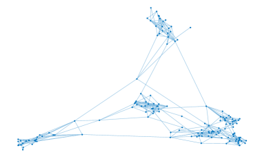
Figure 3: Topology of a simulated (sparse) network

5.1 Image Denoising

Problem formulations: We consider denoising a $512\times 512$ pixels image of a fishing boat (USC, 1997)$-$see Fig. 5(a). We simulate a cluster computer network composed of $150$ nodes (computers). Denoting by $\mathbf{F}_{0}$ and $\mathbf{F}$ the noise-free and corrupted image, respectively, the SNR (in dB) is defined as $\text{SNR}\triangleq 20\cdot\log({||\text{vec}(\mathbf{F}_{0})||_{2}}/{\sqrt{\text{MSE}}})$ while the Peak SNR (in dB) is defined as $\text{PSNR}\triangleq 20\cdot\log({\max_{i}(\text{vec}(\mathbf{F}_{0}))_{i}}/{\sqrt{\text{MSE}}})$, where MSE is the Mean-Squared-Error between $\mathbf{F}_{0}$ and $\mathbf{F}$. The fishing boat image is corrupted by additive white Gaussian noise, so that $\text{SNR}=15$ dB and $\text{PSNR}=20.34$ dB.

To perform the denoising task, we consider the elastic net sparse DL formulation (3). We extract 255,150 square sliding $s\times s$ pixel patches ($s=8$) and aggregate the vectorized extracted patches in a single data matrix $\mathbf{S}$ of size $64\times 255,150$. The size of the dictionary is $s^{2}\times s^{2}=64\times 64$; the data matrix is equally distributed across the $150$ nodes, resulting in sparse representation matrices $\mathbf{X}_{i}$ of size $64\times 1701$ ($K=64$ and $n_{i}=1701$). The total number of optimization variables is then $16,333,696$. The free parameters $\lambda$, $\mu$ and $\alpha$ in (3) are set to $\lambda=1/s$, $\mu=\lambda$ and $\alpha=1$, respectively.

Algorithms and tuning: We tested: i) two instances of the D⁴L Algorithm, corresponding to two alternative choices of the surrogate functions; ii) the Prox-PDA-IP algorithm (Zhao et al., 2016), adapted to problem (3) (only on undirected networks); iii) the ATC algorithm (Chainais and Richard, 2013); and iv) the centralized K-SVD algorithm (Elad and Aharon, 2006) (KSVD-Box v13 package), used as a benchmark. More specifically, the two instances of the D⁴L Algorithm are:

• Plain D⁴L: $\tilde{h}_{i}$ is chosen as in (16) (the original function) and $\tilde{f}_{i}$ as in (15);

• Linearized D⁴L: $\tilde{h}_{i}$ is given by (17) (first-order approximation) and $\tilde{f}_{i}$ is given by (15).

The rest of the parameters in both instances of D⁴L is set as: $\gamma^{\nu}=\gamma^{\nu-1}(1-\epsilon\gamma^{\nu-1})$, with $\gamma^{0}=0.5$ and $\epsilon=10^{-2}$; $\tau^{\nu}_{D,i}=10$; and $\tau^{\nu}_{X,i}=\max(L_{\nabla{X_{i}}}(\mathbf{U}_{(i)}^{\nu}),1)$ [cf. (24)].

Our adaptation of the Prox-PDA-IP algorithm to Problem (3) is summarized in Algorithm 2. The difference with the original version in (Zhao et al., 2016) are: i) the elastic net penalty is used in the objective function for the $\mathbf{X}_{i}$’s variables, instead of the $\ell_{1}$-norm and $\ell_{2}$-norm ball constraints; and ii) the variables $\mathbf{D}_{(i)}$’s are constrained in $\mathcal{D}\triangleq\{\mathbf{D}\,:\,||\mathbf{D}\mathbf{e}_{k}||_{2}\leq\alpha,\,k=1,2,\ldots,K\}$ rather than using the $\ell_{2}$-norm regularization in the objective function. The other symbols used in Algorithm 2 are: i) the incidence matrix of $\mathcal{G}$, denoted by $\mathbf{M}=(M_{ei})_{e,i}\in\mathbb{R}^{E\times I}$, with $E\triangleq|\mathcal{E}|$; ii) the matrices $\boldsymbol{\Omega}_{e}^{\nu}\in\mathbb{R}^{M\times K}$, $e=1,...,E$, which are the $\nu$-th iterate of the dual matrix variables $\boldsymbol{\Omega}_{e}\in\mathbb{R}^{M\times K}$, as introduced in the original Prox-PDA-IP; and iii) $\{\beta^{\nu}\}_{\nu\in\mathbb{N}_{+}}$ is the increasing penalty parameter, set to $\beta^{\nu}=0.002\nu$.

$\textbf{Initialization}:\mathbf{D}_{(i)}^{0}\in\mathcal{D},~{}\mathbf{X}_{i}^{0}\in\mathcal{X}_{i}$, $\boldsymbol{\Omega}^{0}=\mathbf{0}$;
S1. If $(\mathbf{D}_{(i)}^{\nu},\mathbf{X}_{i}^{\nu})_{i}$ satisfies stopping criterion: STOP;
S2. Each agent $i$ computes $\theta_{i}^{\nu}=||\mathbf{D}_{(i)}^{\nu}\mathbf{X}_{i}^{\nu}-\mathbf{S}_{i}||^{2}_{F}$ and:

1. $\displaystyle\mathbf{X}_{i}^{\nu+1}=\underset{\mathbf{X}_{i}\in\mathbb{R}^{K\times n_{i}}}{\text{argmin}}f_{i}(\mathbf{D}_{(i)}^{\nu},\mathbf{X}_{i})+g_{i}(\mathbf{X}_{i})+\frac{\beta^{\nu+1}\theta_{i}^{\nu}}{2}||\mathbf{X}_{i}-\mathbf{X}_{i}^{\nu}||_{F}^{2}+\frac{\beta^{\nu+1}}{2}||\mathbf{D}_{(i)}^{\nu}(\mathbf{X}_{i}-\mathbf{X}_{i}^{\nu})||_{F}^{2}$;

2. $\displaystyle{\mathbf{D}}_{(i)}^{\nu+1}=\underset{\mathbf{D}_{(i)}\in\mathcal{D}}{\text{argmin}}~{}~{}f_{i}(\mathbf{D}_{(i)},\mathbf{X}_{i}^{\nu+1})+\textstyle\sum_{e=1}^{E}M_{ei}\left\langle\boldsymbol{\Omega}_{e}^{\nu},\mathbf{D}_{(i)}\right\rangle$

3. $+\beta^{\nu+1}\left(d_{i}||\mathbf{D}_{(i)}||_{F}^{2}-\big{\langle}\mathbf{D}_{(i)},(d_{i}-1)\mathbf{D}_{(i)}^{\nu}+\textstyle\sum_{j\in\mathcal{N}_{i}}\mathbf{D}_{(j)}^{\nu}\big{\rangle}\right)$;

4. $\boldsymbol{\Omega}^{\nu+1}_{e}=\boldsymbol{\Omega}^{\nu}_{e}+\beta^{\nu+1}\sum_{i=1}^{I}M_{ei}\mathbf{D}_{(i)}^{\nu+1},\quad\forall e=(i,j)\in\mathcal{E}$;

S3. Set $\nu+1\to\nu$, and go to S1.

Algorithm 2 : Prox-PDA-IP algorithm (Zhao et al., 2016)

All the algorithms are initialized to the same value: $\mathbf{D}_{(i)}^{0}$’s coincide with randomly (uniformly) chosen columns of $\mathbf{S}_{(i)}$’s whereas all $\mathbf{X}_{i}^{0}$’s are set to zero.

While the subproblems solved at each iteration $\nu$ in Linearized D⁴L admit a closed-form$-$see (23) and (22)$-$in both Plain D⁴L and ATC, the update of the dictionary has the closed form expression (22), but the update of the private variables calls for the solution of a LASSO problem (cf. Sec. 3.1). For both Plain D⁴L and ATC, the LASSO subproblems at iteration $\nu$ are solved using the (sub)gradient algorithm, with the following tuning. A diminishing step-size is used, set to $\gamma^{r}=\gamma^{r-1}(1-\epsilon\gamma^{r-1})$, where $\gamma^{0}=0.9$, $\epsilon=10^{-3}$, and $r$ denotes the inner iteration index. A warm start is used for the subgradient algorithm: the initial points are set to $\mathbf{X}^{\nu}_{i}$, where $\nu$ is the iteration index of the outer loop. We terminate the subgradient algorithm in the inner loop when $J^{r}_{i}\leq 10^{-6}$, with

$$J^{r}_{i}\triangleq\left\lVert\mathbf{X}^{\nu,r}_{i}-\frac{s}{1+s}\,\mathcal{T}_{\frac{1}{s}}\left(\mathbf{X}^{\nu,r}_{i}-\left(\nabla_{X_{i}}f_{i}(\mathbf{U}_{(i)}^{\nu},\mathbf{X}^{\nu,r}_{i})+\tau_{X,i}^{\nu}\left(\mathbf{X}^{\nu,r}_{i}-\mathbf{X}^{\nu}_{i}\right)\right)\right)\right\rVert_{\infty,\infty},$$

where $\mathbf{X}^{\nu,r}_{i}$ denotes the value of $\mathbf{X}_{i}$ at the $r$-th inner iteration and outer iteration $\nu$; and $\mathcal{T}_{\theta}(x)\triangleq\max(|x|-\theta,0)\cdot\text{sign}(x)$ is the soft-thresholding operator, applied to the matrix argument componentwise. In all our simulations, we observed that the above accuracy was reached within 30 (inner) iterations of the subgradient algorithm.

In the Prox-PDA-IP scheme, Step S2 (cf. Algorithm 2) calls for the solution of two subproblems, including a LASSO problem. As for Plain D⁴L and ATC, we used the (projected) (sub)-gradient algorithm (with the same diminishing step-size rule) to solve the subproblems; we terminated the inner loop when the length between two consecutive iterates of the (projected) (sub)-gradient algorithm goes for the first time below $10^{-6}$.

We simulated both undirected and directed static graphs. In the former case, there is no need of the $\phi$-variables and, in the second equation of (12) [and (13)], the terms $(\phi_{j}^{\nu}\,a^{\nu}_{ij})/\phi_{i}^{\nu+1}$ reduce to $a_{ij}$. The weights $a_{ij}$ are chosen according to the Metropolis-Hasting rule (Xiao et al., 2007); the resulting matrix $\mathbf{A}^{\nu}=[a_{ij}]_{ij}$ is thus time-invariant and doubly stochastic. When the graph is directed, we use the update of the $\phi_{i}^{\nu}$’s as in (12), with the weights $a_{ij}^{\nu}$ chosen according to the push-sum protocol (Kempe et al., 2003) (cf. Sec. 3.1.3).

Convergence speed and quality of the reconstruction: In the first set of simulations, we considered an undirected graph composed of 150 nodes, clustered in 6 groups of 25 (see Fig. 3). Starting from this topology, we kept adding random edges till a connected graph was obtained. Specifically, an arc is added between two nodes in the same cluster (resp. different clusters) with probability $p_{1}=0.2$ (resp. $p_{2}=2\times 10^{-3}$).
In Fig. 4 we plot the objective function value [subplot on the left], the consensus disagreement $e^{\nu}$ as in (30) [subplot in the center], and the distance from stationarity $\Delta^{\nu}$ as in (28) [subplot on the right] versus the number of message exchanges, achieved by Plain D⁴L, Linearized D⁴L, Prox-PDA-IP, and ATC. Note that the number of messages exchanged in the ATC algorithm at iteration $\nu$ coincides with $\nu$ whereas for Prox-PDA-IP and the D⁴L schemes is $2\nu$ (recall that the latter schemes employ two steps of communications per iteration). The figures clearly show that both versions of D⁴L are much faster than Prox-PDA-IP and ATC (or, equivalently, they require fewer information exchanges). Moreover, ATC does not seem to reach a consensus on the local copies of the dictionary, while Prox-PDA-IP and D⁴L schemes reach an agreement quite soon. In Fig. 5, we plot the reconstructed images along with their PSNR and MSE, obtained by the algorithms, when terminated after 1000 message exchanges. The figures clearly show superior performance of D⁴L over its competitors. Also, the values of PSNR and MSE achieved by D⁴L are comparable with those obtained by (centralized) K-SVD (KSVD-Box v13 package).

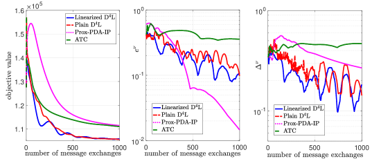
Figure 4: Denoising problem – D⁴L, Prox-PDA-IP and ATC algorithms: objective value [subplot on the left], consensus disagreement [subplot in the center], and distance from stationarity $\Delta^{\nu}$ [cf. (26)] [subplot on the right] vs. number of message exchanges.

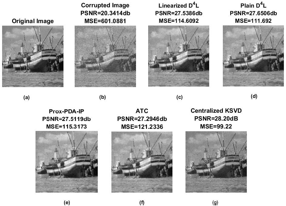
Figure 5: Denoising outcome. (a): original image; (b): corrupted image; (c)-(f): denoising achieved by D⁴L, Prox-PDA-IP and ATC terminated after 1000 message exchanges; and (g): denoising achieved by centralized K-SVD (KSVD-Box v13).

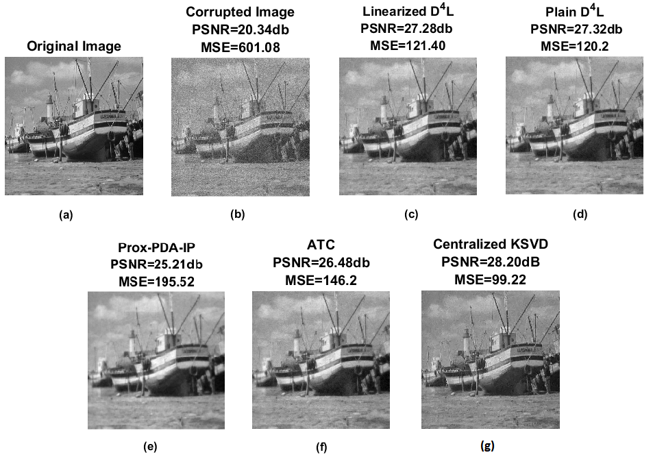
Figure 6: Denoising outcome. (a): original image; (b): corrupted image; (c)-(f): denoising achieved by D⁴L, Prox-PDA-IP and ATC terminated after 200 message exchanges; and (g): denoising achieved by centralized K-SVD (KSVD-Box v13).

A closer look at Fig. 4 shows that a significant decay on the objective function occurs in the first 200 message exchanges. It is then interesting to check the quality of the reconstructed images, achieved by the algorithms if terminated then. In Fig. 6, we report the images and values of PSNR and MSE obtained by terminating the schemes after 200 message exchanges (we also plot the benchmark obtained by K-SVD, run till optimality). The figure shows that both versions of D⁴L attain high quality solutions even if terminated after few message exchanges while ATC and Prox-PDA-IP lag behind. This means that, in practice, there is no need to run D⁴L till very low values of $e^{\nu}$ and $\Delta^{\nu}$ are achieved.

Since the algorithms do not have the same cost-per-iteration, to get further insights into the performance of these schemes, we also compare them in terms of running time. In Table 2, we report the averaged elapsed time to execute one iteration of all algorithms. We considered the same setting as in the previous figures, but we terminated all algorithms after 273 seconds, which corresponds to the time for the fastest algorithm (i.e. Linearized D⁴L) to perform 200 message exchanges [cf. Fig. 6]. The associated reconstructed images are shown in Fig. 7. Once again, these results clearly show that the linearized D⁴L scheme significantly outperforms Prox-PDA-IP and ATC. Also, Linearized D⁴L performs considerably better than Plain D⁴L, when terminated early; the explanation is in Table 2 which shows that the time of one iteration of the former algorithm is much shorter than that of Plain D⁴L.

Algorithm	Average Time per Iteration (sec)
Linearized D4L	2.862
Plain D4L	11.328
Prox-PDA-IP	30.98
ATC	9.838

Table 2: D⁴L vs. Prox-PDA-IP and ATC: Average computation time per iteration

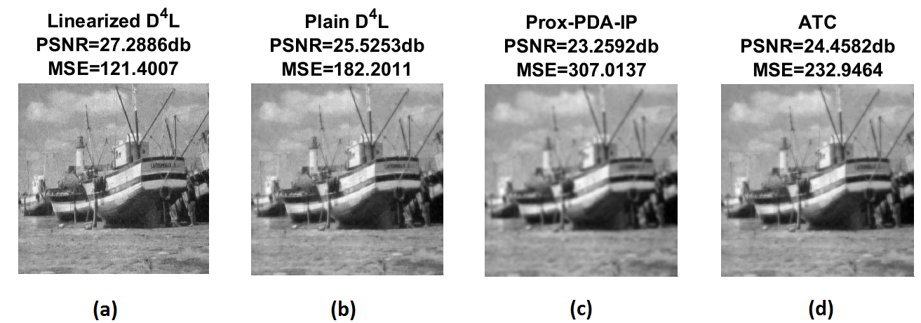
Figure 7: Denoising outcome. (a): Linearized D⁴L; (b): Plain D⁴L; (c): Prox-PDA-IP; (d) ATC; all terminated after after 273 seconds run-time (corresponding to 200 message exchanges of the Linearized D⁴L).

Impact of the graph topology and connectivity: We study now the influence of the topology and graph connectivity on the performance of the algorithms. We consider directed, static graphs. We generated 5 instances of digraphs, with different connectivity, according to the following procedure. There are $500$ nodes ($I=500$), which are clustered in $n_{c}=50$ clusters, each of them containing $10=I/n_{c}$ nodes. Each node has an outgoing arc to another node in the same cluster with probability $p_{1}$ while $p_{2}$ is the probability of an outgoing arc to a node in a different cluster. We chose the values of $p_{1}$ and $p_{2}$, as in Table 3; we simulated three scenarios, namely: N1 corresponds to a “highly” connected network, N3 describes a “poorly” connected scenario, and N2 is an intermediate case. For each scenario, we generated 5 random instances (if a generated graph was not strongly connected we discarded it and generated a new one) and then ran Plain and Linearized D⁴L and ATC on the resulting 15 graphs. Recall that ATC was not designed to work on directed networks. We thus modified it by using our new consensus protocol (but not the gradient tracking mechanism); we term it Modified ATC.

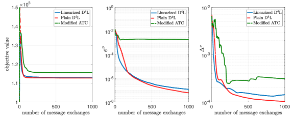
(a)

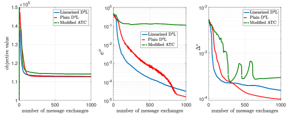
(b)

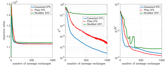
(c)

Figure 8: Denoising problem–D⁴L and Modified ATC algorithms: objective value [subplots on the left], consensus disagreement [subplots in the center], and distance from stationarity $\Delta^{\nu}$ [cf. (26)] [subplots on the right] vs. number of message exchanges. Comparison over three network settings [cf. Table 3]: N1 [subplots (a)], N2 [subplots (b)], and N3 [subplots (c)].

Network #	$I$	$n_{c}$	$p_{1}$	$p_{2}$
N1	500	50	0.9	0.9
N2	500	50	0.1	0.01
N3	500	50	0.05	0.01

Table 3: Network setting

In Fig. 8 we plot the average value of the objective function [subplot on the left], the consensus disagreement $e^{\nu}$ [subplot in the center], and the distance from stationarity $\Delta^{\nu}$ [subplot on the right], achieved by Plain D⁴L, Linearized D⁴L, and Modified ATC, versus the number of message exchanges, for the three scenarios N1 [subplot (a)], N2 [subplot (b)] and N3 [subplot (c)]. The average is taken over the aforementioned 5 digraph realizations. While also this batch of tests confirms the better behavior of D⁴L schemes over ATC, it is interesting to observe that there seems to be little influence of the degree of connectivity on the behavior of Linearized and Plain D⁴L. The only aspect for which a reasonable influence can be seen is on consensus. In fact, with respect to consensus, Linearized D⁴L seems to improve over Plain D⁴L, when connectivity decreases. This has a natural interpretation. Plain D⁴L solves much more accurate subproblems at each iteration and this is, in some sense useless, especially in early iterations, when information has not spread across the network. It seems clear that the less connected the graph, the more time information needs to spread. Therefore, in scenario N1, the two methods are almost equivalent and, looking at consensus error, we see that initially Linearized D⁴L is better than Plain D⁴L, but soon, as information spreads, Plain D⁴L becomes, even if slightly, better than Linearized D⁴L. The same behavior can be observed for scenario N2, but this time the initial advantage of Linearized D⁴L is larger and the switching point is reached much later. This is consistent with the fact that information needs more time to spread and therefore solving the accurate subproblem is not advantageous. If one passes to N3, where connectivity is very loose, there is no switching point within the first 1000 message exchanges.

5.2 Biclustering

Biclustering has been shown to be useful in several applications, including biology, information retrieval, and data mining; see, e.g., (Madeira and Oliveira, 2004).

Problem Formulation: We consider a Biclustering problem in the form (6), applied to genetic information. We solved the problem simulating a networked computer cluster composed of 500 nodes (see Table 3). The genetic data is borrowed from (Lee et al., 2010) (centered and normalized): the data matrix $\mathbf{S}$ of size $56\times 12,625$ ($M=56$ and $N=12,625$) contains microarray gene expressions of 56 patients (rows); each patient is either identified to be normal (Normal) or belonging to one of the following three types of lung cancer: pulmonary carcinoid tumors (Carcinoid), colon metastases (Colon), and small cell carcinoma (SmallCell). We considered the unsupervised instance of the problem, meaning that none of the a-priori information about the type of patients’ cancer is used to perform biclustering. Following the numerical experiments of (Lee et al., 2010), we seek rank-$3$ sparse matrices $\mathbf{X}_{i}$, and the data matrix $\mathbf{S}$ is equally distributed across the 500 nodes, resulting thus in $K=3$ and $n_{i}=26$. The total number of variables is then $39,168$. The other parameters are set as follows: $\alpha=1$, $\lambda_{X}=\mu_{X}=0.1$, and $\lambda_{D}=\mu_{D}=0.1$.

Algorithms and tuning: We tested the instance of D⁴L where $\tilde{f}_{i}$ and $\tilde{h}_{i}$ are chosen according to (14) and (16), respectively. The rationale behind this choice is to exploit the extra structure of the original function $f_{i}$, plus, in case of $\tilde{f}_{i}$, there is no certain benefit in using the linear approximation (15) as it does not lead to any closed form solution of the subproblem (8). Note that the Prox-PDA-IP scheme is not applicable here since the network is directed.

The other parameters of the algorithm are set to: $\gamma^{\nu}=\gamma^{\nu-1}(1-\epsilon\gamma^{\nu-1})$, with $\gamma^{0}=0.2$ and $\epsilon=10^{-2}$; and $\tau^{\nu}_{D,i}=100$ and $\tau^{\nu}_{X,i}=\max(L_{\nabla{X_{i}}}(\mathbf{U}_{(i)}^{\nu}),100)$. We term such an instance of D⁴L Plain D⁴L. We compared Plain D⁴L with the following algorithms: i) (a modified version of) the distributed ATC algorithm (Chainais and Richard, 2013), where the optimization of $\mathbf{D}$ is adjusted to solve (6) (the elastic-net penalty is added), and the consensus mechanism is modified with our new consensus protocol to handle directed network topologies; we termed this instance Modified ATC; and ii) the centralized SSVD algorithm proposed in Lee et al. (2010) (implemented using the MATLAB code provided by the authors), to benchmark the results obtained by the distributed algorithms. All the distributed algorithm are initialized setting each $\mathbf{X}_{i}^{0}=\mathbf{0}$, and each $\mathbf{D}_{(i)}^{0}$ equal to some randomly chosen columns of $\mathbf{S}_{i}$.

In D⁴L, the subproblems (8) and (11) at iteration $\nu$ do not have a closed form solution; they are solved using the projected (sub)gradient algorithm, with diminishing step-size $\gamma^{r}=\gamma^{r-1}(1-\epsilon\gamma^{r-1})$, where $\gamma^{0}=0.9$, $\epsilon=10^{-3}$, and $r$ denotes the inner iteration index. A warm start is used for the projected subgradient algorithm; the initial points are set to $\mathbf{D}_{(i)}^{\nu}$ and $\mathbf{X}^{\nu}_{i}$ in problems (8) and (11), respectively, where $\nu$ is the iteration index of the outer loop. We terminate the projected subgradient algorithm solving (8) and (11) when $J^{r}_{D,i}\triangleq\|\widehat{\mathbf{D}}^{\nu,r}_{(i)}-\mathbf{D}^{\nu,r}_{(i)}\|_{\infty,\infty}\leq 10^{-6}$ and $J^{r}_{X,i}\triangleq\|\widehat{\mathbf{X}}^{\nu,r}_{i}-\mathbf{X}^{\nu,r}_{i}\|_{\infty,\infty},\leq 10^{-6}$, respectively, where

$$\widehat{\mathbf{D}}^{\nu,r}_{(i)} \triangleq\underset{\mathbf{D}_{(i)}\in\mathcal{D}}{\text{argmin}}\left\langle\nabla_{D}f_{i}(\mathbf{D}_{(i)}^{\nu,r},\mathbf{X}^{\nu}_{i})+I\boldsymbol{\Theta}_{(i)}^{\nu}-\nabla_{D}f_{i}(\mathbf{D}_{(i)}^{\nu},\mathbf{X}^{\nu}_{i})+\tau_{D,i}^{\nu}\big{(}\mathbf{D}^{\nu,r}_{(i)}-\mathbf{D}^{\nu}_{(i)}\big{)},\mathbf{D}_{(i)}-\mathbf{D}_{(i)}^{\nu,r}\right\rangle\vspace{-0.2cm}$$

$$\qquad\qquad\qquad\qquad\qquad\qquad\qquad\qquad\qquad\qquad\qquad+\frac{100}{2}\left\lVert\mathbf{D}_{(i)}-\mathbf{D}_{(i)}^{\nu,r}\right\rVert^{2}+G\left(\mathbf{D}_{(i)}\right),\vskip 6.0pt plus 2.0pt minus 2.0pt$$

$$\widehat{\mathbf{X}}^{\nu,r}_{i} \triangleq\underset{\mathbf{X}_{i}\in\mathbb{R}^{K\times n_{i}}}{\text{argmin}}\left\langle\nabla_{X_{i}}f_{i}(\mathbf{U}_{(i)}^{\nu},\mathbf{X}^{\nu,r}_{i})+\tau_{X,i}^{\nu}\left(\mathbf{X}^{\nu,r}_{i}-\mathbf{X}^{\nu}_{i}\right),\mathbf{X}_{i}-\mathbf{X}_{i}^{\nu,r}\right\rangle$$

$$\qquad\qquad\qquad\qquad\qquad\qquad\qquad\qquad\qquad\qquad\qquad+\frac{100}{2}\left\lVert\mathbf{X}_{i}-\mathbf{X}_{i}^{\nu,r}\right\rVert^{2}+g_{i}\left(\mathbf{X}_{i}\right),$$

with $\mathbf{D}^{\nu,r}_{(i)}$ and $\mathbf{X}^{\nu,r}_{i}$ denoting the value of $\mathbf{D}_{(i)}$ and $\mathbf{X}_{i}$ at the $\nu$-th outer and $r$-th inner iteration, respectively. In all our simulations, the above accuracy was reached within 50 (inner) iterations of the projected subgradient algorithm.

Convergence speed and quality of the reconstruction: We simulated 3 directed static network topologies, namely: N1-N3, as given in Table 3. In Fig. 9 we plot he average value of the objective function [subplot on the left], the consensus disagreement $e^{\nu}$ [subplot in the center], and the distance from stationarity $\Delta^{\nu}$ [subplot on the right], achieved by Plain D⁴L and Modified ATC, versus the number of message exchanges, for the three scenarios N1 [subplot (a)], N2 [subplot (b)] and N3 [subplot (c)]. The average is taken over 5 digraph realizations. Fig. 9 shows that Plain D⁴L algorithm attains satisfactory merit values in all network scenarios, while Modified ATC fails to reach consensus/convergence, even in highly connected networks. The poor performance of Modified ATC seem mainly due to the incapability of locking the consensus.

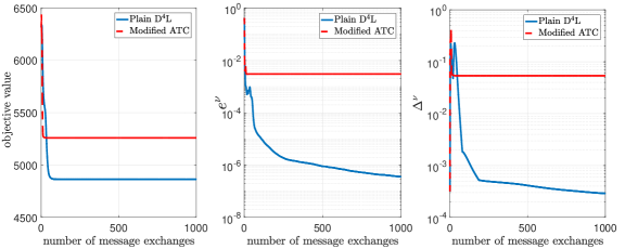
(a)

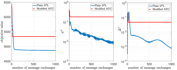
(b)

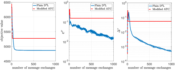
(c)

Figure 9: Biclustering problem–Plain D⁴L and Modified ATC algorithms: objective value [subplots on the left], consensus disagreement [subplots in the center], and distance from stationarity $\Delta^{\nu}$ [cf. (26)] [subplots on the right] vs. number of message exchanges. Comparison over three network settings [cf. Table 3]: N1 [subplots (a)], N2 [subplots (b)], and N3 [subplots (c)].

In order to assess the quality of the solutions achieved by the three algorithms, we employ the following procedure. Given the limit point (up to the fixed accuracy) $\mathbf{D}^{\infty}$ of the algorithm under consideration, patients’ information is in form of (unlabeled clusters of) data points $\{\mathbf{D}_{m,:}^{\infty}\}_{m=1}^{56}$, where $\mathbf{D}_{m,:}^{\infty}$ denotes the $m$-th row of $\mathbf{D}^{\infty}$ and represents an individual patient. In order to compare $\mathbf{D}^{\infty}$ with the labeled ground truth, we need to tag labels to the clustered points of $\mathbf{D}^{\infty}$. To do so, we run the K-means clustering algorithm on $\{\mathbf{D}_{m,:}^{\infty}\}_{m=1}^{56}$. Specifically, we first run K-means 100 times and, in each run, we perform a preliminary clustering using 10% of the points (randomly chosen). Then, among the 100 obtained clustering configurations, we picked the one with the smallest “within-cluster sum of point-to-centroid distances”. Finally, we assign to each cluster the label associated with the most populated type of cancer in the cluster. Denoting the ground truth classes by $\{\mathcal{C}_{i}\}_{i=1}^{4}$ (recall that there are 4 classes/types of cancer), where each $\mathcal{C}_{i}$ consists of the group of patients with the same type of cancer, and by $\{\widetilde{\mathcal{C}}_{i}\}_{i=1}^{4}$ the clustering obtained by the procedure described above applied to the outcome $\mathbf{D}^{\infty}$ of the simulated algorithms, we measure the quality of the clustering by the Jaccard index, defined as

$$J=\frac{\left|\bigcup_{i}\left(\mathcal{C}_{i}\cap\widetilde{\mathcal{C}}_{i}\right)\right|}{\sum_{i}\left|\mathcal{C}_{i}\cup\widetilde{\mathcal{C}}_{i}\right|}.\vspace{-0.2cm}$$

Clearly $0\leq J\leq 1$, and the higher the index value, the better the quality of the clustering.

In Table 4, we report the average and Maximum Absolute Deviation (MAD) of the Jaccard indices from their average, computed over the aforementioned 5 realizations of the three graph topologies, as in Table 3 (see also Fig. 9). The values in the table clearly show that Plain D⁴L achieves better results than those produced by Modified ATC or centralized methods. Moreover, the value of the Jaccard index from Plain D⁴L does not depend on the specific network topology. which is not the case for Modified ATC.

Network #	Plain D4L	Modified ATC	Lee et al. (2010)
N1	0.8983/0	0.7778/0	–
N2	0.8983/0	0.7045/0.3218	–
N3	0.8983/0	0.7892/0.0172	–
Centralized	–	–	0.7231/–

Table 4: Biclustering problem$-$Average/MAD of Jaccard indices over 5 realizations of digraphs.

5.3 Non-negative Sparse Coding (NNSC) and Sparse PCA (SPCA)

Problem Formulation: We consider the Non-negative Sparse Coding (NSC) formulation (7) (Hoyer, 2004) and the Sparse PCA problem (6) (Mairal et al., 2010). For both formulations, we run experiments using the following two datasets:

• MIT-CBCL face database #1 (Sung, 1996): a pool of $N=2,429$ vectorized face images of size $19\times 19$ pixels each (i.e. $M=361$);

• The VOC 2006 database (Everingham et al., 2010): a pool of $N=10,000$ vectorized natural image patches of size $16\times 16$ pixels each (i.e. $M=256$).

Consistently with (Mairal et al., 2010), the free parameters are set as:

• NNSC (7): $K=49$, $\lambda=\mu=1/\sqrt{M}$, and $\alpha=1$;

• Sparse PCA (6): $K=49$, $\lambda_{X}=\mu_{X}=1/\sqrt{M}$, $\lambda_{D}=\mu_{D}=1/\sqrt{M}$, and $\alpha=1$.

The total number of variables for the above optimization problems are 136,710 for the MIT-CBCL dataset, and 502,544 for the VOC 2006 dataset.

We simulated the communication network as static directed graphs of size $I$, clustered in $n_{c}$ groups, where each node has an outgoing arc to another node in the same cluster with probability $p_{1}$, while $p_{2}$ is the probability of an outgoing arc to a node in a different cluster. We run our tests over 6 different network scenarios, with various size $I$ and probability pair $(p_{1},p_{2})$, as given in Table 5. Note that if $N/I$ is not an integer, we pad zero columns to the data matrix $\mathbf{S}$ so that all the agents own equal-size partitions $\mathbf{S}_{i}$’s, thus $n_{i}=\left\lceil N/I\right\rceil$ in both problems (6) and (7).

Network #	$I$	$n_{c}$	$p_{1}$	$p_{2}$
N4	10	2	0.9	0.3
N5	10	2	0.2	0.1
N6	50	5	0.9	0.3
N7	50	5	0.2	0.1
N8	250	10	0.9	0.3
N9	250	10	0.2	0.1

Table 5: Network setting for the NNSC and Sparse PCA problems.

5.3.1 Non-negative Sparse Coding

Algorithms and tuning: We test the Plain D⁴L, with $\tilde{f}_{i}$ and $\tilde{h}_{i}$ chosen according to (15) and (16), respectively. The other parameters of the algorithm are set to: $\gamma^{\nu}=\gamma^{\nu-1}(1-\epsilon\gamma^{\nu-1})$, with $\gamma^{0}=0.2$ and $\epsilon=10^{-2}$; and $\tau^{\nu}_{D,i}=10$ and $\tau^{\nu}_{X,i}=\max(L_{\nabla{X_{i}}}(\mathbf{U}_{(i)}^{\nu}),10)$. We compare the proposed scheme with a modified version of ATC, equipped with our new consensus protocol, implementable on directed networks. All the distributed algorithm are initialized setting $\mathbf{X}_{i}^{0}=\mathbf{0}$ and $\mathbf{D}_{(i)}^{0}$ equal to some randomly chosen columns of $\mathbf{S}_{i}$. Both Plain D⁴L and Modified ATC call for solving a LASSO problem in updating the private variables (cf. Sec. 3.1); the update of the dictionary has instead a closed form expression, see (22). For both Plain D⁴L and Modified ATC, the LASSO subproblems at iteration $\nu$ are solved using the projected (sub)gradient algorithm with diminishing step-size $\gamma^{r}=\gamma^{r-1}(1-\epsilon\gamma^{r-1})$, where $\gamma^{0}=0.9$, $\epsilon=10^{-3}$, and $r$ denoting the inner iteration index. We terminate the projected subgradient algorithm in the inner loop when $J_{X,i}^{r}\triangleq\|\widehat{\mathbf{X}}^{\nu,r}_{i}-\mathbf{X}^{\nu,r}_{i}\|_{\infty,\infty}\leq 10^{-4}$, where

$$\widehat{\mathbf{X}}^{\nu,r}_{i}\triangleq\underset{\mathbf{X}_{i}\in\mathcal{X}_{i}}{\text{argmin}}\left\langle\nabla_{X_{i}}f_{i}(\mathbf{U}_{(i)}^{\nu},\mathbf{X}^{\nu,r}_{i})+\tau_{X,i}^{\nu}\left(\mathbf{X}^{\nu,r}_{i}-\mathbf{X}^{\nu}_{i}\right),\mathbf{X}_{i}-\mathbf{X}_{i}^{\nu,r}\right\rangle+\frac{1}{2}\left\lVert\mathbf{X}_{i}-\mathbf{X}_{i}^{\nu,r}\right\rVert^{2}+g_{i}\left(\mathbf{X}_{i}\right),\vspace{-0.2cm}$$

and $\mathbf{X}^{\nu,r}_{i}$ denotes the value of $\mathbf{X}_{i}$ at the $\nu$-th outer and $r$-th inner iteration. In all our simulations, the above accuracy was reached within 30 (inner) iterations of the projected subgradient algorithm.

Convergence speed and quality of the reconstruction: We run the Plain D⁴L and Modified ATC algorithms over different network settings, as listed in Table 5, and we terminated them after 1500 message exchanges. We replicated the tests for 5 independent realizations and we reported the average of the final values of the objective function, the consensus disagreement, and the distance from stationarity in Table 6 and Table 7, for the MIT-CBCL and VOC 2006 datasets, respectively. In Fig. 10 and Fig. 11 (for MIT-CBCL and VOC 2006 datasets, respectively), we plot the average value (over the aforementioned 5 graph realizations) of the objective function [subplot on the left], the consensus disagreement $e^{\nu}$ [subplot in the center], and the distance from stationarity $\Delta^{\nu}$ [subplot on the right], versus number of message exchanges, for the two extreme network scenarios N4 [subplot (a)] and N9 [subplot (b)]. These results show that the proposed Plain D⁴L significantly outperforms the Modified ATC algorithm. They also show a remarkable stability of Plain D⁴L with respect to the simulated network graphs, which is not observed for the Modified ATC, whose performance deteriorates significantly going from N4 to N9.

Network #	objective value	consensus disagreement	distance from stationarity
N4	169.8/171.9	9.17e-7/2.9e-4	4.7e-4/8.8e-2
N5	169.9/172.2	4.5e-6/6.7e-4	5.3e-4/9.8e-2
N6	169.8/177.2	2.4e-7/1.9e-4	5.1e-4/6.3e-2
N7	169.9/177.3	1.1e-6/6.3e-4	5.5e-4/6.1e-2
N8	169.8/191.0	2.1e-7/1.2e-4	5.1e-4/2.2e-2
N9	169.8/190.9	5.8e-7/3.1e-4	6.6e-4/1.1e-2

Table 6: NNSC problem (MIT-CBCL dataset)–Plain D⁴L/Modified ATC algorithms: objective value, consensus disagreement, and distance from stationarity obtained after 1500 message exchanges.

Network #	objective value	consensus disagreement	distance from stationarity
N4	845.2/848.8	2.9e-6/1.3e-4	1.1e-3/4.1e-3
N5	845.9/850.1	1.5e-5/5.3e-4	1.5e-3/6.1e-3
N6	844.8/879.5	5.7e-7/2.2e-4	1.3e-3/4.4e-2
N7	844.5/879.3	1.9e-6/1.2e-3	1.3e-3/3.9e-2
N8	844.8/941.2	5.6e-7/1.5e-4	1.6e-3/4.8e-2
N9	845.0/941.8	1.5e-6/3.6e-4	1.1e-3/5.1e-2

Table 7: NNSC problem (VOC 2006 dataset)–Plain D⁴L/Modified ATC algorithms: objective value, consensus disagreement, and distance from stationarity obtained after 1500 message exchanges.

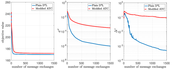
(a)

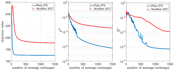
(b)

Figure 10: NNSC problem (MIT-CBCL dataset)–Plain D⁴L and Modified ATC algorithms: objective value [subplots on the left], consensus disagreement [subplots in the center], and distance from stationarity $\Delta^{\nu}$ [cf. (26)] [subplots on the right] vs. number of message exchanges. Comparison over the network settings N4 [subplots (a)] and N9 [subplots (b)] (cf. Table 5).

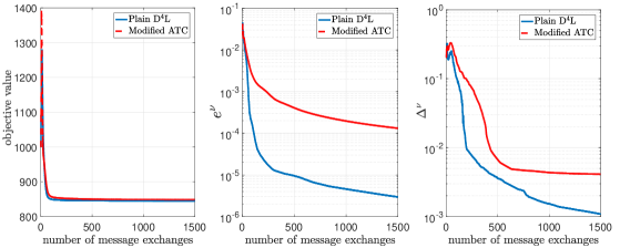
(a)

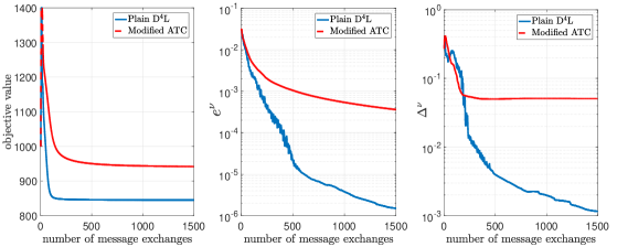
(b)

Figure 11: NNSC problem (VOC 2006 dataset)–Plain D⁴L and Modified ATC algorithms: objective value [subplots on the left], consensus disagreement [subplots in the center], and distance from stationarity $\Delta^{\nu}$ [cf. (26)] [subplots on the right] vs. number of message exchanges. Comparison over the network settings N4 [subplots (a)] and N9 [subplots (b)] (cf. Table 5).

5.3.2 Sparse Principal Component Analysis (SPCA)

Algorithms and tuning: We test the same D⁴L version as used in the Biclustering experiments (cf. Subsec. 5.2), i.e., $\tilde{f}_{i}$ and $\tilde{h}_{i}$ are chosen according to (14) and (16), respectively; we set $\gamma^{\nu}=\gamma^{\nu-1}(1-\epsilon\gamma^{\nu-1})$, with $\gamma^{0}=0.2$ and $\epsilon=10^{-2}$; and $\tau^{\nu}_{D,i}=10$ and $\tau^{\nu}_{X,i}=\max(L_{\nabla{X_{i}}}(\mathbf{U}_{(i)}^{\nu}),10)$. We term it Plain D⁴L. We compare Plain D⁴L with a modified version of the ATC algorithm, which has been adapted to solve (6) and equipped with our new consensus protocol to handle directed network topologies. All the distributed algorithm are initialized, setting $\mathbf{X}_{i}^{0}=\mathbf{0}$ and $\mathbf{D}_{(i)}^{0}$ equal to some randomly chosen columns of $\mathbf{S}_{i}$. The subproblems (8) and (11) at iteration $\nu$ are solved using the projected (sub)gradient algorithm; the setting is the same as that used in the Biclustering problem (cf. Subsec. 5.2). We terminate the projected subgradient algorithm in the inner loop when $J^{r}_{D,i}\leq 10^{-4}$ (in solving subproblem (8)) and $J^{r}_{X,i}\leq 10^{-4}$ (in solving subproblem (11)), where $J^{r}_{D,i}$ and $J^{r}_{X,i}$ are defined as those in Subsec. 5.2. In all our simulations, the above accuracy was reached within 30 (inner) iterations of the projected subgradient algorithm.

Convergence speed and quality of the reconstruction: We test the Plain D⁴L and the Modified ATC in different network settings, as listed in Table 5. The setting of the experiments and the averaging procedure of the reported values is the same of those used for the NNSC problem. The results of our experiments are reported in Table 8 and Figure 12 for the MIT-CBCL dataset; and in Table 9 and Figure 13 for the VOC 2006 dataset. The behaviors or the algorithms are very similar to those described in the NNSC case and confirm all previous observations.

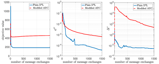
(a)

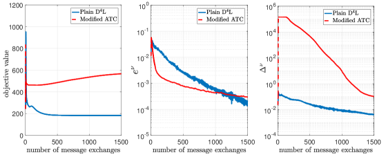
(b)

Figure 12: SPCA problem (MIT-CBCL dataset)–Plain D⁴L and Modified ATC algorithms: objective value [subplots on the left], consensus disagreement [subplots in the center], and distance from stationarity $\Delta^{\nu}$ [cf. (26)] [subplots on the right] vs. number of message exchanges. Comparison over the network settings N4 [subplots (a)] and N9 [subplots (b)] (cf. Table 5).

Network #	objective value	consensus disagreement	distance from stationarity
N4	181.9/453.1	3.5e-5/6.1e-4	2.2e-3/21.39
N5	185.1/446.4	2.6e-5/1.5e-3	1.3e-3/136.2
N6	182.7/517.3	5.2e-6/4.3e-4	1.3e-3/1.2e-1
N7	186.3/512.0	2.3e-5/9.2e-4	1.4e-3/1.18
N8	181.9/566.0	4.0e-5/1.7e-4	2.6e-3/1.5e-1
N9	182.6/566.9	1.7e-4/2.9e-4	4.2e-3/1.0e-1

Table 8: SPCA problem (MIT-CBCL dataset)–Plain D⁴L/Modified ATC algorithms: objective value, consensus disagreement, and distance from stationarity obtained after 1500 message exchanges.

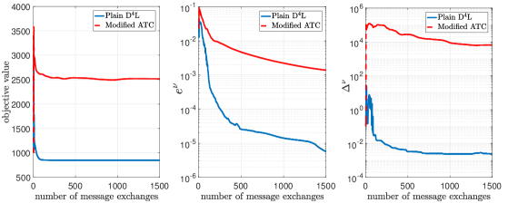
(a)

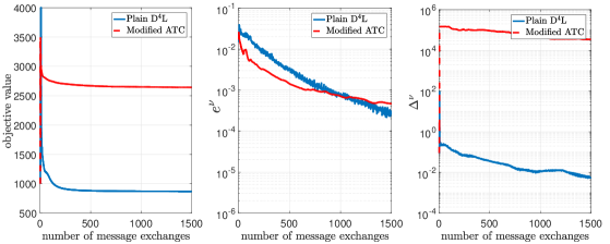
(b)

Figure 13: SPCA problem (VOC 2006 dataset)–Plain D⁴L and Modified ATC algorithms: objective value [subplots on the left], consensus disagreement [subplots in the center], and distance from stationarity $\Delta^{\nu}$ [cf. (26)] [subplots on the right] vs. number of message exchanges. Comparison over the network settings N4 [subplots (a)] and N9 [subplots (b)] (cf. Table 5).

Network #	objective value	consensus disagreement	distance from stationarity
N4	849.3/2516.0	5.7e-6/1.3e-3	2.3e-3/6532
N5	866.0/2533.6	1.8e-5/3.5e-3	2.0e-3/1.3e+4
N6	864.8/2621.0	7.2e-6/4.3e-4	3.4e-3/1.7e+4
N7	859.1/2624.1	5.3e-5/1.1e-3	2.4e-3/1.6e+4
N8	872.7/2643.2	6.6e-5/2.3e-4	1.1e-2/2.9e+4
N9	869.1/2642.0	2.3e-4/4.6e-4	5.6e-3/3.4e+4

Table 9: SPCA problem (VOC 2006 dataset)–Plain D⁴L/Modified ATC algorithms: objective value, consensus disagreement, and distance from stationarity obtained after 1500 message exchanges.

6 Conclusions

This paper studied a fairly general class of distributed dictionary learning problems over time-varying multi-agent networks, with arbitrary topologies. We proposed the first decentralized algorithmic framework$-$the D⁴L Algorithm$-$with provable convergence for this class of problems. Numerical experiments showed promising performance of our scheme with respect to state-of-the-art distributed methods.

Acknowledgments

The work of Daneshmand, Sun, and Scutari has been supported by the the National Science Foundation (NSF grants CIF 1564044 and CAREER Award No. 1555850) and the the Office of Naval Research (ONR Grant N00014-16-1-2244). The work of Facchinei has been partially supported by the Italian Ministry of Education, Research and University, under the PLATINO (PLATform for INnOvative services in future internet) PON project (Grant Agreement no. PON01$\_$01007).

Appendix A Appendix

In this section we prove the major results of the paper, Theorems 2 and 3. We begin rewriting the D⁴L Algorithm in an equivalent vector-matrix form (cf. Sec. A.1), which is more suitable for the analysis. Theorem 2 and Theorem 3 are then proved in Sec. A.2 and Sec. A.3, respectively. Some miscellanea results supporting the main proofs are collected in Appendix A.4. Table 10 below summarizes the symbols appearing in the proofs.

Symbol	Definition	Member of	Reference
$\overline{\mathbf{D}}_{\boldsymbol{\phi}^{\nu}}$	$(1/I)\sum_{i=1}^{I}\phi_{i}^{\nu}\,\mathbf{D}_{(i)}^{\nu}$	$\mathcal{D}\subseteq\mathbb{R}^{M\times K}$	(41)
$\overline{\mathbf{U}}_{\boldsymbol{\phi}^{\nu}}$	$(1/I)\sum_{i=1}^{I}\phi_{i}^{\nu}\,\mathbf{U}_{(i)}^{\nu}$	$\mathcal{D}\subseteq\mathbb{R}^{M\times K}$	(41)
$\widetilde{\mathbf{D}}^{\nu}$	$[\widetilde{\mathbf{D}}_{(1)}^{\nu\intercal},\widetilde{\mathbf{D}}_{(2)}^{\nu\intercal},\ldots,\widetilde{\mathbf{D}}_{(I)}^{\nu\intercal}]^{\intercal}$	$\mathbb{R}^{M\times KI}$	(34)
${\mathbf{U}}^{\nu}$	$[{\mathbf{U}}_{(1)}^{\nu\intercal},{\mathbf{U}}_{(2)}^{\nu\intercal},\ldots,{\mathbf{U}}_{(I)}^{\nu\intercal}]^{\intercal}$	$\mathbb{R}^{M\times KI}$	(34)
$\boldsymbol{{\Theta}}^{\nu}$	$[\boldsymbol{{\Theta}}_{(1)}^{\nu\intercal},\boldsymbol{{\Theta}}_{(2)}^{\nu\intercal},\ldots,\boldsymbol{{\Theta}}_{(I)}^{\nu\intercal}]^{\intercal}$	$\mathbb{R}^{M\times KI}$	(34)
$\mathbf{G}^{\nu}$	$[\nabla_{D}f_{1}(\mathbf{D}_{(1)}^{\nu},\mathbf{X}^{\nu}_{1})^{\intercal},~{}\ldots~{},~{}\nabla_{D}f_{I}(\mathbf{D}_{(I)}^{\nu},\mathbf{X}^{\nu}_{I})^{\intercal}]^{\intercal}$	$\mathbb{R}^{M\times KI}$	(34)
$\mathbf{W}^{\nu}$	$(w_{ij}^{\nu})_{i,j=1}^{I}=(a^{\nu}_{ij}\,\phi_{j}^{\nu}/\phi_{i}^{\nu+1})_{i,j=1}^{I}=(\boldsymbol{\Phi}^{\nu+1})^{-1}\mathbf{A}^{\nu}\boldsymbol{\Phi}^{\nu}$	$\mathbb{R}^{I\times I}$	(35)
$\mathbf{W}^{\nu:l}$	$\mathbf{W}^{\nu}\cdot\mathbf{W}^{\nu-1}\cdots\mathbf{W}^{l},\quad\nu>l$	$\mathbb{R}^{I\times I}$	(44)
$\widehat{\mathbf{W}}^{\nu}$	$\mathbf{W}^{\nu}\otimes\mathbf{I}_{M}$	$\mathbb{R}^{MI\times MI}$	(36)
$\widehat{\mathbf{W}}^{\nu:l}$	$\mathbf{W}^{\nu:l}\otimes\mathbf{I}_{M},\quad\nu>l$	$\mathbb{R}^{MI\times MI}$	(44)
$\boldsymbol{\phi}^{\nu}$	$[\phi_{1}^{\nu},\phi_{2}^{\nu},\ldots,\phi_{I}^{\nu}]^{\intercal}$	$\mathbb{R}^{I}$	(34)
$\boldsymbol{\Phi}^{\nu}$	$\mathrm{diag}\left(\boldsymbol{\phi}^{\nu}\right)$	$\mathbb{R}^{I\times I}$	(34)
$\widehat{\boldsymbol{\Phi}}^{\nu}$	$\boldsymbol{\Phi}^{\nu}\otimes\mathbf{I}_{M}$	$\mathbb{R}^{MI\times MI}$	(36)
$\mathbf{J}_{\boldsymbol{\phi}^{\nu}}$	$(1/I)\mathbf{1}\boldsymbol{\phi}^{\nu\intercal}$	$\mathbb{R}^{I\times I}$	(45)
$\widehat{\mathbf{J}}_{\boldsymbol{\phi}^{\nu}}$	$\mathbf{J}_{\boldsymbol{\phi}^{\nu}}\otimes\mathbf{I}_{M}$	$\mathbb{R}^{MI\times MI}$	(45)

Table 10: Table of notation (appendix)

A.1 D⁴L in vector-matrix form

We rewrite Algorithm 1 in a more convenient vector-matrix form. To do so, we introduce the following notation. Recalling the definitions of $\widetilde{\mathbf{D}}^{\nu}_{(i)}$ [cf. (8)], $\mathbf{U}_{(i)}^{\nu}$ [cf. (10)], $\phi_{i}^{\nu}$ [cf. (12)], and $\boldsymbol{{\Theta}}^{\nu}_{(i)}$ [cf. (13)], define the corresponding aggregate quantities

$$\widetilde{\mathbf{D}}^{\nu}\triangleq[\widetilde{\mathbf{D}}_{(1)}^{\nu\intercal},\widetilde{\mathbf{D}}_{(2)}^{\nu\intercal},\ldots,\widetilde{\mathbf{D}}_{(I)}^{\nu\intercal}]^{\intercal},$$ (34)

$$\mathbf{U}^{\nu}\triangleq[\mathbf{U}_{(1)}^{\nu\intercal},\mathbf{U}_{(2)}^{\nu\intercal},\ldots,\mathbf{U}_{(I)}^{\nu\intercal}]^{\intercal},$$

$$\boldsymbol{\phi}^{\nu}\triangleq[\phi_{1}^{\nu},\phi_{2}^{\nu},\ldots,\phi_{I}^{\nu}]^{\intercal},\quad\boldsymbol{\Phi}^{\nu}\triangleq\mathrm{diag}\left(\boldsymbol{\phi}^{\nu}\right)$$

$$\boldsymbol{{\Theta}}^{\nu}\triangleq[\boldsymbol{{\Theta}}_{(1)}^{\nu\intercal},\boldsymbol{{\Theta}}_{(2)}^{\nu\intercal},\ldots,\boldsymbol{{\Theta}}_{(I)}^{\nu\intercal}]^{\intercal},$$

$$\mathbf{G}^{\nu}\triangleq\bigg{[}\nabla_{D}f_{1}(\mathbf{D}_{(1)}^{\nu},\mathbf{X}^{\nu}_{1})^{\intercal},~{}\nabla_{D}f_{2}(\mathbf{D}_{(2)}^{\nu},\mathbf{X}^{\nu}_{2})^{\intercal},~{}\ldots~{},~{}\nabla_{D}f_{I}(\mathbf{D}_{(I)}^{\nu},\mathbf{X}^{\nu}_{I})^{\intercal}\bigg{]}^{\intercal},$$

where $\mathrm{diag}(\mathbf{x})$ is a diagonal matrix whose diagonal entries are the components of the vector $\mathbf{x}$. Combining the weights $a_{ij}^{\nu}$ and the variables $\phi_{i}^{\nu}$ in the update of $\mathbf{D}_{(i)}^{\nu}$ [cf. (12)] in the single coefficient

$$w_{ij}^{\nu}\triangleq\dfrac{a_{ij}^{\nu}\phi_{j}^{\nu}}{\sum_{k}a_{ik}^{\nu}\phi_{k}^{\nu}},$$

we define the weight matrix $\mathbf{W}^{\nu}$, whose entries are $[\mathbf{W}^{\nu}]_{i,j}=w_{ij}^{\nu}$. Note that $\mathbf{W}^{\nu}$ has the same zero-pattern of $\mathbf{A}^{\nu}$, and the following properties hold (the latter under Assumption F)

$$\mathbf{W}^{\nu}=\big{(}\boldsymbol{\Phi}^{\nu+1}\big{)}^{-1}\mathbf{A}^{\nu}\boldsymbol{\Phi}^{\nu},\quad\mathrm{and}\quad\mathbf{W}^{\nu}\mathbf{1}=\mathbf{1}.$$ (35)

Finally, we define the following “augmented” matrices

$$\widehat{\mathbf{W}}^{\nu}\triangleq\mathbf{W}^{\nu}\otimes\mathbf{I}_{M}\quad\text{and}\quad\widehat{\boldsymbol{\Phi}}^{\nu}\triangleq\boldsymbol{\Phi}^{\nu}\otimes\mathbf{I}_{M},$$ (36)

where $\mathbf{I}_{M}$ is the $M$-by-$M$ identity matrix.

Using the above notation, the main iterates of the D⁴L Algorithm, i.e., (10), (12), and (13), can be rewritten in compact form as

$$~{}~{}\quad\qquad\mathbf{U}^{\nu}=\mathbf{D}^{\nu}+\gamma^{\nu}(\widetilde{\mathbf{D}}^{\nu}-\mathbf{D}^{\nu}),$$ (37)

$$~{}\qquad\qquad\qquad\boldsymbol{\phi}^{\nu+1}=\mathbf{A}^{\nu}\boldsymbol{\phi}^{\nu},$$ (38)

$$\qquad\qquad\qquad\mathbf{D}^{\nu+1}=\widehat{\mathbf{W}}^{\nu}\mathbf{U}^{\nu},$$ (39)

$$\boldsymbol{{\Theta}}^{\nu+1}=\widehat{\mathbf{W}}^{\nu}\boldsymbol{{\Theta}}^{\nu}+\big{(}\widehat{\boldsymbol{\Phi}}^{\nu+1}\big{)}^{-1}\left(\mathbf{G}^{\nu+1}-\mathbf{G}^{\nu}\right).$$ (40)

Instrumental to the analysis of the consensus disagreement are the following weighted average quantities:

$$\overline{\mathbf{D}}_{\boldsymbol{\phi}^{\nu}}\triangleq\dfrac{1}{I}\sum_{i=1}^{I}\phi_{i}^{\nu}\,\mathbf{D}_{(i)}^{\nu},\quad\overline{\mathbf{U}}_{\boldsymbol{\phi}^{\nu}}\triangleq\dfrac{1}{I}\sum_{i=1}^{I}\phi_{i}^{\nu}\,\mathbf{U}_{(i)}^{\nu}.$$ (41)

Using (12), (41) and the column stochasticity of $\mathbf{A}^{\nu}$ (cf. Assumption F3), it is not difficult to check that

$$\overline{\mathbf{D}}_{\boldsymbol{\phi}^{\nu+1}}=\overline{\mathbf{U}}_{\boldsymbol{\phi}^{\nu}},$$ (42)

which, together with (10), leads to the following dynamics for $\overline{\mathbf{D}}_{\boldsymbol{\phi}^{\nu}}$:

$$\overline{\mathbf{D}}_{\boldsymbol{\phi}^{\nu+1}}=\overline{\mathbf{D}}_{\boldsymbol{\phi}^{\nu}}+\frac{\gamma^{\nu}}{I}\sum_{i=1}^{I} \phi_{i}^{\nu}\left(\widetilde{\mathbf{D}}^{\nu}_{(i)}-\mathbf{D}_{(i)}^{\nu}\right).$$ (43)

A.2 Proof of Theorem 2

We prove Theorem 2 in the following order (consistent with the statements in the theorem):

Step 1–Asymptotic consensus & related properties:

We prove that consensus is asymptotically achieved, that is, $\lim_{\nu\rightarrow\infty}e^{\nu}=0$ [statement (a)], along with some properties on related quantities, which will be used in the other steps–see Sec. A.2.1;

Step 2–Boundedness of the iterates:

We prove that the sequence $\big{\{}\big{(}\mathbf{D}^{\nu},\mathbf{X}^{\nu}\big{)}\big{\}}_{\nu}$ generated by the algorithm is bounded [statement (b-i)]–see Sec. A.2.2;

Step 3–Decrease of $\{U(\overline{\mathbf{D}}^{\nu},\mathbf{X}^{\nu})\}_{\nu}$:

We study the properties of $\{U(\overline{\mathbf{D}}^{\nu},\mathbf{X}^{\nu})\}_{\nu}$ [statement (b-ii)]–see Sec. A.2.3;

Step 4–Vanishing X-stationarity:

We prove that $\lim_{\nu\rightarrow\infty}\Delta_{X}(\overline{\mathbf{D}}^{\nu},\mathbf{X}^{\nu})=0$ [statement (b-iii)]–see Sec. A.2.4;

Step 5–Vanishing liminf D-stationarity:

We prove $\liminf_{\nu\rightarrow\infty}\Delta_{D}(\overline{\mathbf{D}}^{\nu},\mathbf{X}^{\nu})=0$ [statement (b-iv)]–see Sec. A.2.5;

Step 6–Vanishing D-stationarity:

Finally, we prove $\lim_{\nu\rightarrow\infty}\Delta_{D}(\overline{\mathbf{D}}^{\nu},\mathbf{X}^{\nu})=0$ [statement (b’)]–see Sec. A.2.6.

A.2.1 Step 1–Asymptotic consensus and related properties

1) Preliminaries: To analyze the dynamics of the consensus disagreement, we first introduce the following product matrices and their augmented counterparts: Given $\mathbf{W}^{\nu}$ [cf. (35)], and $\nu,l\in\mathbb{N}_{+}$, with $\nu\geq l$, let

$$~{}\mathbf{W}^{\nu:l}\triangleq\begin{cases}\mathbf{W}^{\nu}\cdot\mathbf{W}^{\nu-1}\cdots\mathbf{W}^{l},&\nu>l,\\ \mathbf{W}^{\nu},&\nu=l,\\ \mathbf{0}_{I},&\nu<l,\end{cases}\quad\text{and}\quad\widehat{\mathbf{W}}^{\nu:l}\triangleq\mathbf{W}^{\nu:l}\otimes\mathbf{I}_{M}.$$ (44)

Define also the weight-average matrices

$$\mathbf{J}_{\boldsymbol{\phi}^{\nu}}\triangleq\frac{1}{I}\mathbf{1}\boldsymbol{\phi}^{\nu\intercal},\quad\widehat{\mathbf{J}}_{\boldsymbol{\phi}^{\nu}}\triangleq\mathbf{J}_{\boldsymbol{\phi}^{\nu}}\otimes\mathbf{I}_{M}.$$ (45)

For notational simplicity, when $\boldsymbol{\phi}^{\nu}=\mathbf{1}$, we use $\mathbf{J}$ instead of $\mathbf{J}_{\boldsymbol{\phi}^{\nu}}$ and $\widehat{\mathbf{J}}\triangleq\mathbf{J}\otimes\mathbf{I}_{M}$. Using (35) and (41), it is not difficult to check that the following hold:

$$\quad\widehat{\mathbf{J}}_{\boldsymbol{\phi}^{\nu}}\mathbf{D}^{\nu}=\mathbf{1}\otimes\overline{\mathbf{D}}_{\boldsymbol{\phi}^{\nu}},$$ (46)

$$\widehat{\mathbf{J}}_{\boldsymbol{\phi}^{\nu+1}}\widehat{\mathbf{W}}^{\nu:l}=\widehat{\mathbf{J}}\,\widehat{\boldsymbol{\Phi}}^{l}=\widehat{\mathbf{J}}_{\boldsymbol{\phi}^{l}}.$$ (47)

The dynamics of the consensus disagreement $e^{\nu}$ boils down to studying the decay of $\|\mathbf{W}^{\nu:l}-\mathbf{J}_{\boldsymbol{\phi}^{l}}\|_{2}$ (this will be clear in the proof of Proposition 5 below). The following lemma shows that $\mathbf{W}^{\nu:l}$ converges geometrically to $\mathbf{J}_{\boldsymbol{\phi}^{l}}$, as $\nu\to\infty$.

Lemma 4 (Scutari and Sun (2018)-Lemma 4.13, Ch. 3.4.2.5)

Let $\{\mathcal{G}^{\nu}\}_{\nu}$ be a sequence of digraphs satisfying Assumption B; let $\{\mathbf{A}^{\nu}\}_{\nu}$ be a sequence of matrices satisfying Assumption F; and let $\{\mathbf{W}^{\nu}\}_{\nu}$ be the sequence of matrices defined in (35). Then, there holds

$$\left\lVert\mathbf{W}^{\nu:l}-\mathbf{J}_{\boldsymbol{\phi}^{l}}\right\rVert_{2}\leq c_{W}\,(\rho)^{\nu-l+1},\quad\forall\nu\geq l,\,\nu,l\in\mathbb{N}_{+},$$

where $c_{W}>0$ is a (proper) constant, and $\rho\in(0,1)$ is defined as

$$\rho=\left(1-\tilde{\kappa}^{-(I-1)B}\right)^{\frac{1}{B(I-1)}}<1,$$ (48)

with $\tilde{\kappa}=\kappa^{IB+1}/I$; and $\kappa$ is defined in Assumption F.

Furthermore, the sequence $\{\phi_{i}^{\nu}\}_{\nu}$ satisfies

$$\underline{\epsilon}_{\phi}\triangleq\inf_{\nu\in\mathbb{N}_{+}}\left(\min_{1\leq i\leq I}\phi^{\nu}_{i}\right)\geq\kappa^{IB},\quad\text{and}\quad\bar{\epsilon}_{\phi}\triangleq\sup_{\nu\in\mathbb{N}_{+}}\left(\max_{1\leq i\leq I}\phi^{\nu}_{i}\right)\leq I-(I-1)\kappa^{IB}.$$ (49)

If all the matrices $\mathbf{A}^{\nu}$ are doubly-stochastic, then $\underline{\epsilon}_{\phi}=\bar{\epsilon}_{\phi}=1$.

2) Proof of $\lim_{\nu\rightarrow\infty}e^{\nu}=0$. Using (30), we can write

$$e^{\nu}\overset{(a)}{\leq}K\left\lVert\mathbf{D}^{\nu}-\mathbf{1}\otimes\overline{\mathbf{D}}^{\nu}\right\rVert_{F} \overset{(b)}{\leq}K\left\lVert\mathbf{D}^{\nu}-\mathbf{1}\otimes\overline{\mathbf{D}}_{\boldsymbol{\phi}^{\nu}}\right\rVert_{F}+K\,\sqrt{I}\left\lVert\overline{\mathbf{D}}^{\nu}-\overline{\mathbf{D}}_{\boldsymbol{\phi}^{\nu}}\right\rVert_{F}$$ (50)

$$\overset{(c)}{\leq}2K\left\lVert\mathbf{D}^{\nu}-\mathbf{1}\otimes\overline{\mathbf{D}}_{\boldsymbol{\phi}^{\nu}}\right\rVert_{F},$$

where (a) follows from the equivalence of norms; (b) is due to the triangle inequality; and in (c) we used $\sum_{i=1}^{I}a_{i}\leq\sqrt{I}||\mathbf{a}||$, with $\mathbf{a}=(a_{i})_{i=1}^{I}\in\mathbb{R}^{I}$.

The following proposition concludes the proof of statement (a), proving that $\|\mathbf{D}^{\nu}-\mathbf{1}\otimes\overline{\mathbf{D}}_{\boldsymbol{\phi}^{\nu}}\|_{F}$ is square summable, along with some additional properties on related quantities.

Proposition 5

In the above setting, there hold:

$$\quad\lim_{\nu\rightarrow\infty}~{}||\mathbf{D}^{\nu}-\mathbf{1}\otimes\overline{\mathbf{D}}_{\boldsymbol{\phi}^{\nu}}||_{F}=0,$$ (51)

$$\lim_{\nu\rightarrow\infty}\,\sum_{t=1}^{\nu}~{}||\mathbf{D}^{t}-\mathbf{1}\otimes\overline{\mathbf{D}}_{\boldsymbol{\phi}^{t}}||_{F}^{2}<\infty;$$ (52)

$$\lim_{\nu\rightarrow\infty}\,\sum_{t=1}^{\nu}~{}||\mathbf{U}^{t}-\mathbf{1}\otimes\overline{\mathbf{U}}_{\boldsymbol{\phi}^{t}}||_{F}^{2}<\infty.$$ (53)

Proof  To prove (51), let us first expand $\mathbf{D}^{\nu}-\mathbf{1}\otimes\overline{\mathbf{D}}_{\boldsymbol{\phi}^{\nu}}$ as follows: for any $\nu\geq 1$,

$$\mathbf{D}^{\nu} \,\overset{\eqref{D_weighted_avg_stackingMat}}{=}\,\widehat{\mathbf{W}}^{\nu-1}\mathbf{U}^{\nu-1}=\widehat{\mathbf{W}}^{\nu-1}\mathbf{D}^{\nu-1}+\widehat{\mathbf{W}}^{\nu-1}\left(\mathbf{U}^{\nu-1}-\mathbf{D}^{\nu-1}\right)$$ (54)

$$\,{=}\,\widehat{\mathbf{W}}^{\nu-1:0}\mathbf{D}^{0}+\sum_{t=0}^{\nu-1}\widehat{\mathbf{W}}^{\nu-1:t}\left(\mathbf{U}^{t}-\mathbf{D}^{t}\right),$$

where the last equality follows from induction and the definition of $\widehat{\mathbf{W}}^{\nu:l}$ [cf. (44)]. Similarly, we expand the subtrahend as

$$\mathbf{1}\otimes\overline{\mathbf{D}}_{\boldsymbol{\phi}^{\nu}} \overset{\eqref{D_avg_stackingMat}}{=}\widehat{\mathbf{J}}_{\boldsymbol{\phi}^{\nu}}\mathbf{D}^{\nu}\overset{\eqref{rewrite_1}}{=}\widehat{\mathbf{J}}_{\boldsymbol{\phi}^{\nu}}\left(\widehat{\mathbf{W}}^{\nu-1:0}\mathbf{D}^{0}+\sum_{t=0}^{\nu-1}\widehat{\mathbf{W}}^{\nu-1:t}\left(\mathbf{U}^{t}-\mathbf{D}^{t}\right)\right)$$ (55)

$$\overset{\eqref{colStochW_avgMat_eq}}{=}\widehat{\mathbf{J}}\left(\mathbf{D}^{0}+\sum_{t=0}^{\nu-1}\widehat{\boldsymbol{\Phi}}^{t}\left(\mathbf{U}^{t}-\mathbf{D}^{t}\right)\right).$$

Subtracting (55) from (54) and using (37), yields

$$\left\lVert\mathbf{D}^{\nu}-\mathbf{1}\otimes\overline{\mathbf{D}}_{\boldsymbol{\phi}^{\nu}}\right\rVert_{F}\leq \left\lVert\widehat{\mathbf{W}}^{\nu-1:0}-\widehat{\mathbf{J}}\right\rVert_{2}\left\lVert\mathbf{D}^{0}\right\rVert_{F}+\sum_{t=0}^{\nu-1}\gamma^{t}\left\lVert\widehat{\mathbf{W}}^{\nu-1:t}-\widehat{\mathbf{J}}_{\phi^{t}}\right\rVert_{2}\left\lVert\widetilde{\mathbf{D}}^{t}-\mathbf{D}^{t}\right\rVert_{F}$$ (56)

$$\overset{(a)}{\leq} c_{1}(\rho)^{\nu}+c_{2}~{}\sum_{t=0}^{\nu-1}~{}\gamma^{t}~{}(\rho)^{\nu-t}\stackrel{{\scriptstyle[}}{{\nu}}\rightarrow\infty]{(b)}{\longrightarrow}0,$$

for some finite constants $c_{1},c_{2}>0$, where (a) is due to Lemma 4 and the boundedness of $\{||\widetilde{\mathbf{D}}^{\nu}-\mathbf{D}^{\nu}||\}_{\nu}$; and (b) follows from Lemma 13(a) in Appendix A.4.

Let us now proceed to prove (52). Using (56), we have

$$\lim_{\nu\rightarrow\infty}\,\sum_{t=1}^{\nu}\left\lVert\mathbf{D}^{t}-\mathbf{1}\otimes\overline{\mathbf{D}}_{\boldsymbol{\phi}^{t}}\right\rVert_{F}^{2}\leq\lim_{\nu\rightarrow\infty}\,\sum_{t=1}^{\nu}\left(c_{1}(\rho)^{t}+c_{2}~{}\sum_{l=0}^{t-1}~{}\gamma^{l}~{}(\rho)^{t-l}\right)^{2}$$

$$\overset{(a)}{\leq}\frac{2c_{1}^{2}}{1-(\rho)^{2}}+2\,c_{2}^{2}\lim_{\nu\rightarrow\infty}\,\sum_{t=1}^{\nu}\sum_{l=0}^{t-1}\sum_{k=0}^{t-1}\gamma^{l}\gamma^{k}(\rho)^{t-k}(\rho)^{t-l}$$

$$\overset{(b)}{\leq}\frac{2c_{1}^{2}}{1-(\rho)^{2}}+c_{2}^{2}\lim_{\nu\rightarrow\infty}\,\sum_{t=1}^{\nu}\sum_{l=0}^{t-1}(\gamma^{l})^{2}(\rho)^{t-l}\sum_{k=0}^{t-1}(\rho)^{t-k}+c_{2}^{2}\lim_{\nu\rightarrow\infty}\,\sum_{t=1}^{\nu}\sum_{k=0}^{t-1}(\gamma^{k})^{2}(\rho)^{t-k}\sum_{l=0}^{t-1}(\rho)^{t-l}$$

$$\leq\frac{2c_{1}^{2}}{1-(\rho)^{2}}+\frac{2c_{2}^{2}}{1-\rho}\lim_{\nu\rightarrow\infty}\,\sum_{t=1}^{\nu}\sum_{l=0}^{t-1}(\gamma^{l})^{2}(\rho)^{t-l}\,\overset{(c)}{<}\infty,$$

where in (a) and (b) we used $(a+b)^{2}\leq 2(a^{2}+b^{2})$ and $ab\leq(a^{2}+b^{2})/2$, respectively, and (c) is due to Lemma 13(b) (cf. Appendix A.4).

We prove now (53). Using (41) and (37), we get

$$\left\lVert\mathbf{U}^{t}-\mathbf{1}\otimes\overline{\mathbf{U}}_{\boldsymbol{\phi}^{t}}\right\rVert_{F}^{2} =\left\lVert\gamma^{t}\Big{(}\widetilde{\mathbf{D}}^{t}-\mathbf{1}\otimes\dfrac{1}{I}\sum_{i=1}^{I}\phi_{i}^{t}\,\widetilde{\mathbf{D}}_{(i)}^{t}\Big{)}+\left(1-\gamma^{t}\right)\left(\mathbf{D}^{t}-\mathbf{1}\otimes\overline{\mathbf{D}}_{\boldsymbol{\phi}^{t}}\right)\right\rVert_{F}^{2}$$ (57)

$$\leq 2\left(\gamma^{t}\right)^{2}\Big{\|}\widetilde{\mathbf{D}}^{t}-\mathbf{1}\otimes\dfrac{1}{I}\sum_{i=1}^{I}\phi_{i}^{t}\,\widetilde{\mathbf{D}}_{(i)}^{t}\Big{\|}_{F}^{2}+2\left\lVert\mathbf{D}^{t}-\mathbf{1}\otimes\overline{\mathbf{D}}_{\boldsymbol{\phi}^{t}}\right\rVert_{F}^{2},$$

where in the last inequality we used Jensen’s inequality and $(1-\gamma^{t})\leq 1$. Therefore,

$$\lim_{\nu\rightarrow\infty}\,\sum_{t=1}^{\nu}\left\lVert\mathbf{U}^{t}-\mathbf{1}\otimes\overline{\mathbf{U}}_{\boldsymbol{\phi}^{t}}\right\rVert_{F}^{2}\leq\lim_{\nu\rightarrow\infty}2\,c_{3}\sum_{t=1}^{\nu}\left(\gamma^{t}\right)^{2}+\lim_{\nu\rightarrow\infty}2\sum_{t=1}^{\nu}\left\lVert\mathbf{D}^{t}-\mathbf{1}\otimes\overline{\mathbf{D}}_{\boldsymbol{\phi}^{t}}\right\rVert_{F}^{2}\,\overset{(a)}{<}\infty,$$

where $c_{3}$ is a positive finite constant, and (a) follows from Assumption E and (52).  

Remark 6 (On $L_{\nabla{X_{i}}}(\overline{\mathbf{U}}_{\boldsymbol{\phi}^{\nu}})$ and $L_{\nabla{X_{i}}}(\mathbf{U}_{(i)}^{\nu})$)

Recall that $\nabla_{X_{i}}f_{i}(\overline{\mathbf{U}}_{\boldsymbol{\phi}^{\nu}},\bullet)$ is Lipschitz continuous on $\mathcal{X}_{i}$, with constant $L_{\nabla{X_{i}}}(\overline{\mathbf{U}}_{\boldsymbol{\phi}^{\nu}})$ (cf. Assumption A2). Since $||\mathbf{U}_{(i)}^{\nu}-\overline{\mathbf{U}}_{\boldsymbol{\phi}^{\nu}}||_{F}\underset{\nu\rightarrow\infty}{\longrightarrow}0$ [cf. (53), Proposition 5] and $L_{\nabla{X_{i}}}(\mathbf{D})$ is continuous, we have

$$\Big{\lvert}L_{\nabla{X_{i}}}(\overline{\mathbf{U}}_{\boldsymbol{\phi}^{\nu}})-L_{\nabla{X_{i}}}(\mathbf{U}_{(i)}^{\nu})\Big{\rvert}\underset{\nu\rightarrow\infty}{\longrightarrow}0,\quad i=1,2,\ldots I.$$ (58)

A.2.2 Step 2–Boundedness of the iterates

We show that the sequence $\big{\{}\big{(}\mathbf{D}^{\nu},\mathbf{X}^{\nu}\big{)}\big{\}}_{\nu}$ generated by the $D^{4}L$ Algorithm is bounded [statement (b-i)]. We prove the result only for $\tilde{h}_{i}$ given by (17); the proof can be easily tailored to the other choice of $\tilde{h}_{i}$. If the sets $\mathcal{X}_{i}$ are bounded [Assumption A5(i)], the result follows readily. Therefore, we consider next the setting under A5(ii).

Throughout the proof, we will use the following properties of $\tilde{f}_{i}$ and $\tilde{h}_{i}$.

Remark 7

The surrogate functions $\tilde{f}_{i}$ and $\tilde{h}_{i}$ as in Assumption C have the following properties: for all $i=1,2,\ldots,I$,

1. $\tilde{f}_{i}(\bullet;\mathbf{D},\mathbf{X}_{i})$ is strongly convex on $\mathcal{D}$, uniformly with respect to $(\mathbf{D},\mathbf{X}_{i})\in\mathcal{D}\times\mathcal{X}_{i}$, with constant $\tau_{D,i}^{\nu}>0$; and $\nabla_{D}\tilde{f}_{i}(\mathbf{D};\mathbf{D},\mathbf{X}_{i})=\nabla_{D}f_{i}(\mathbf{D},\mathbf{X}_{i})$, for all $(\mathbf{D},\mathbf{X}_{i})\in\mathcal{D}\times\mathcal{X}_{i}$.

2. $\tilde{h}_{i}(\bullet;\mathbf{D},\mathbf{X}_{i})$ is strongly convex on $\mathcal{X}_{i}$, uniformly with respect to $(\mathbf{D},\mathbf{X}_{i})\in\mathcal{D}\times\mathcal{X}_{i}$, with constant $\tau_{X,i}^{\nu}>0$; and $\nabla_{X_{i}}\tilde{h}_{i}(\mathbf{X}_{i};\mathbf{D},\mathbf{X}_{i})=\nabla_{X_{i}}f_{i}(\mathbf{D},\mathbf{X}_{i})$, for all $(\mathbf{D},\mathbf{X}_{i})\in\mathcal{D}\times\mathcal{X}_{i}$.

By the optimality of $\mathbf{X}_{i}^{\nu+1}$ in (11), there exist $\boldsymbol{\Xi}^{0}_{i}\in\partial_{X_{i}}g_{i}(\mathbf{X}^{0}_{i})$ and $\boldsymbol{\Xi}^{\nu+1}_{i}\in\partial_{X_{i}}g_{i}(\mathbf{X}_{i}^{\nu+1})$ such that

$$0 \leq\left\langle\nabla_{X_{i}}\tilde{h}_{i}(\mathbf{X}_{i}^{\nu+1};\mathbf{U}_{(i)}^{\nu},\mathbf{X}_{i}^{\nu})+\boldsymbol{\Xi}_{i}^{\nu+1},\mathbf{X}_{i}^{0}-\mathbf{X}_{i}^{\nu+1}\right\rangle$$

$$=\left\langle\boldsymbol{\Xi}_{i}^{\nu+1}-\boldsymbol{\Xi}^{0}_{i}+\tau_{X,i}^{\nu}(\mathbf{X}_{i}^{\nu+1}-\mathbf{X}^{0}_{i}),\mathbf{X}^{0}_{i}-\mathbf{X}_{i}^{\nu+1}\right\rangle$$

$$\quad+\left\langle\nabla_{X_{i}}f_{i}(\mathbf{U}_{(i)}^{\nu},\mathbf{X}_{i}^{\nu})-\nabla_{X_{i}}f_{i}(\mathbf{U}_{(i)}^{\nu},\mathbf{X}_{i}^{0}),\mathbf{X}^{0}_{i}-\mathbf{X}_{i}^{\nu+1}\right\rangle$$

$$\quad-\left\langle\tau_{X,i}^{\nu}(\mathbf{X}_{i}^{\nu}-\mathbf{X}^{0}_{i}),\mathbf{X}^{0}_{i}-\mathbf{X}_{i}^{\nu+1}\right\rangle$$

$$\quad+\left\langle\nabla_{X_{i}}f_{i}(\mathbf{U}_{(i)}^{\nu},\mathbf{X}_{i}^{0})+\boldsymbol{\Xi}^{0}_{i},\mathbf{X}^{0}_{i}-\mathbf{X}_{i}^{\nu+1}\right\rangle.$$

Using Remark 7(b) and the $\mu_{i}$-strongly convexity of $g_{i}$’s, we obtain

$$(\tau_{X,i}^{\nu}+\mu_{i})\left\lVert\mathbf{X}_{i}^{\nu+1}-\mathbf{X}^{0}_{i}\right\rVert_{F}^{2} \leq\left\langle\tau_{X,i}^{\nu}\mathbf{X}_{i}^{\nu}-\nabla_{X_{i}}f_{i}(\mathbf{U}_{(i)}^{\nu},\mathbf{X}_{i}^{\nu}),\mathbf{X}_{i}^{\nu+1}-\mathbf{X}^{0}_{i}\right\rangle$$ (59)

$$\quad-\left\langle\tau_{X,i}^{\nu}\mathbf{X}^{0}_{i}-\nabla_{X_{i}}f_{i}(\mathbf{U}_{(i)}^{\nu},\mathbf{X}_{i}^{0}),\mathbf{X}_{i}^{\nu+1}-\mathbf{X}^{0}_{i}\right\rangle$$

$$\quad-\left\langle\underbrace{\nabla_{X_{i}}f_{i}(\mathbf{U}_{(i)}^{\nu},\mathbf{X}_{i}^{0})+\boldsymbol{\Xi}^{0}_{i}}_{\triangleq\mathbf{Z}_{i}^{\nu}\in\partial_{X_{i}}U(\mathbf{U}_{(i)}^{\nu},\mathbf{X}^{0}_{i})},\mathbf{X}_{i}^{\nu+1}-\mathbf{X}^{0}_{i}\right\rangle.$$

Define $\Upsilon_{i}^{\nu}(\mathbf{X}_{i})\triangleq\tau_{X,i}^{\nu}\mathbf{X}_{i}-\nabla_{X_{i}}f_{i}(\mathbf{U}_{(i)}^{\nu},\mathbf{X}_{i})$ and rewrite (59) as

$$(\tau_{X,i}^{\nu}+\mu_{i})\,||\mathbf{X}_{i}^{\nu+1}-\mathbf{X}^{0}_{i}||_{F}\leq\left\lVert\Upsilon_{i}^{\nu}(\mathbf{X}^{\nu}_{i})-\Upsilon_{i}^{\nu}(\mathbf{X}^{0}_{i})\right\rVert_{F}+\left\lVert\mathbf{Z}_{i}^{\nu}\right\rVert_{F}.$$ (60)

Since $\mathcal{D}$ is compact and $\mathbf{X}_{i}^{0}$ is given, we have $||\mathbf{Z}_{i}^{\nu}||_{F}\leq B_{Z}$, for all $i$, $\nu\geq 1$, and some finite $B_{Z}>0$. Let us bound next $||\Upsilon_{i}^{\nu}(\mathbf{X}^{\nu}_{i})-\Upsilon_{i}^{\nu}(\mathbf{X}^{0}_{i})||_{F}$. We write

$$\left\lVert\Upsilon_{i}^{\nu}(\mathbf{X}^{\nu}_{i})-\Upsilon_{i}^{\nu}(\mathbf{X}^{0}_{i})\right\rVert_{F}^{2} =(\tau_{X,i}^{\nu})^{2}\left\lVert\mathbf{X}^{\nu}_{i}-\mathbf{X}^{0}_{i}\right\rVert_{F}^{2}+\left\lVert\nabla_{X_{i}}f_{i}(\mathbf{U}_{(i)}^{\nu},\mathbf{X}_{i}^{\nu})-\nabla_{X_{i}}f_{i}(\mathbf{U}_{(i)}^{\nu},\mathbf{X}_{i}^{0})\right\rVert_{F}^{2}$$ (61)

$$\quad-2\tau_{X,i}^{\nu}\left\langle\nabla_{X_{i}}f_{i}(\mathbf{U}_{(i)}^{\nu},\mathbf{X}_{i}^{\nu})-\nabla_{X_{i}}f_{i}(\mathbf{U}_{(i)}^{\nu},\mathbf{X}_{i}^{0}),\mathbf{X}^{\nu}_{i}-\mathbf{X}^{0}_{i}\right\rangle$$

$$\overset{(a)}{\leq}(\tau_{X,i}^{\nu})^{2}\left\lVert\mathbf{X}^{\nu}_{i}-\mathbf{X}^{0}_{i}\right\rVert_{F}^{2}$$

$$\quad+\left(1-\frac{2\tau_{X,i}^{\nu}}{L_{\nabla X_{i}}(\mathbf{U}_{(i)}^{\nu})}\right)\left\lVert\nabla_{X_{i}}f_{i}(\mathbf{U}_{(i)}^{\nu},\mathbf{X}_{i}^{\nu})-\nabla_{X_{i}}f_{i}(\mathbf{U}_{(i)}^{\nu},\mathbf{X}_{i}^{0})\right\rVert_{F}^{2},$$

where in (a) we used the $1/L_{\nabla X_{i}}(\mathbf{U}_{(i)}^{\nu})$-co-coercivity of $\nabla_{X_{i}}f_{i}(\mathbf{U}_{(i)}^{\nu},\bullet)$ [due to the convexity of $f_{i}(\mathbf{U}_{(i)}^{\nu},\bullet)$ and the $L_{\nabla X_{i}}(\mathbf{U}_{(i)}^{\nu})$-Lipschitianity of $\nabla_{X_{i}}f_{i}(\mathbf{U}_{(i)}^{\nu},\bullet)$ (Rockafellar and Wets, 1998, Prop.12.60)], i.e.,

$$\begin{array}[]{ll}\left\langle\nabla_{X_{i}}f_{i}(\mathbf{U}_{(i)}^{\nu},\mathbf{X}_{i})-\nabla_{X_{i}}f_{i}(\mathbf{U}_{(i)}^{\nu},\mathbf{Y}_{i}),\mathbf{X}_{i}-\mathbf{Y}_{i}\right\rangle\geq\\ \hskip 56.9055pt\dfrac{1}{L_{\nabla X_{i}}(\mathbf{U}_{(i)}^{\nu})}\cdot\left\lVert\nabla_{X_{i}}f_{i}(\mathbf{U}_{(i)}^{\nu},\mathbf{X}_{i})-\nabla_{X_{i}}f_{i}(\mathbf{U}_{(i)}^{\nu},\mathbf{Y}_{i})\right\rVert_{F}^{2},\qquad\forall\mathbf{X}_{i},\mathbf{Y}_{i}\in\mathcal{X}_{i}.\end{array}$$

Note that $||\Upsilon_{i}^{\nu}(\mathbf{X}^{\nu}_{i})-\Upsilon_{i}^{\nu}(\mathbf{X}^{0}_{i})||_{F}\leq\tau_{X,i}^{\nu}||\mathbf{X}^{\nu}_{i}-\mathbf{X}^{0}_{i}||_{F}$ as long as $\tau_{X,i}^{\nu}\geq\frac{1}{2}L_{\nabla X_{i}}(\mathbf{U}_{(i)}^{\nu})$, which is satisfied under D1. Therefore, we can bound (60) as

$$(\tau_{X,i}^{\nu}+\mu_{i})||\mathbf{X}_{i}^{\nu+1}-\mathbf{X}^{0}_{i}||_{F}\leq\tau_{X,i}^{\nu}\left\lVert\mathbf{X}^{\nu}_{i}-\mathbf{X}^{0}_{i}\right\rVert_{F}+B_{Z}.$$ (62)

We can now prove that, starting from $\mathbf{X}_{i}^{0}$, the iterates $\mathbf{X}_{i}^{\nu}$ stays in the ball $\mathcal{B}_{i}(R_{i},\mathbf{X}^{0}_{i})\triangleq\{\mathbf{X}_{i}\in\mathbb{R}^{K\times n_{i}}\,:\,\|\mathbf{X}_{i}-\mathbf{X}^{0}_{i}\|_{F}\leq R_{i}\}$, for all $\nu\geq 1$, where $R_{i}\geq{B_{Z}}/{\mu_{i}}$. Let us prove it by induction. Evidently $\mathbf{X}^{0}_{i}\in\mathcal{B}_{i}(R_{i},\mathbf{X}^{0}_{i})$. Let $\mathbf{X}_{i}^{\nu}\in\mathcal{B}_{i}(R_{i},\mathbf{X}^{0}_{i})$; by (62), we get

$$||\mathbf{X}_{i}^{\nu+1}-\mathbf{X}^{0}_{i}||_{F} \,\leq\,\frac{\tau_{X,i}^{\nu}}{\tau_{X,i}^{\nu}+\mu_{i}}\,||\mathbf{X}_{i}^{\nu}-\mathbf{X}^{0}_{i}||_{F}+\frac{B_{Z}}{\tau_{X,i}^{\nu}+\mu_{i}}\,\leq\,R_{i},$$

where the second inequality is due to $\mathbf{X}_{i}^{\nu}\in\mathcal{B}_{i}(R,\mathbf{X}^{0}_{i})$ and $R\geq{B_{Z}}/{\mu}$. Hence $\mathbf{X}_{i}^{\nu+1}\in\mathcal{B}_{i}(R_{i},\mathbf{X}^{0}_{i})$. Therefore, $\mathbf{X}_{i}^{\nu}\in\mathcal{B}_{i}(R_{i},\mathbf{X}^{0}_{i})$, for all $\nu\geq 0$. Since $\mathcal{D}$ is bounded (cf. Assumption A3), it follows that $(\mathbf{D}_{(i)}^{\nu},\mathbf{X}_{i}^{\nu})\in\mathcal{D}\times\mathcal{B}_{i}(R_{i},\mathbf{X}^{0}_{i})$, for all $\nu\geq 0$. $\hfill\square$

Remark 8 (On the Lipschitz continuity of $\nabla f_{i}$’s)

Since $f_{i}$ is $\mathcal{C}^{2}$, a direct consequence of the boundedness of $\big{\{}\big{(}\mathbf{D}^{\nu},\mathbf{X}^{\nu}\big{)}\big{\}}_{\nu}$ is that $\nabla f_{i}$ [the gradient of $f_{i}$ with respect to $(\mathbf{D},\mathbf{X}_{i})$] is Lipschitz continuous on $\mathcal{D}\times\mathcal{B}_{i}(R_{i},\mathbf{X}^{0}_{i})$, that is, there exists some positive finite constant $L_{\nabla,i}$ such that

$$||\nabla f_{i}(\mathbf{D},\mathbf{X}_{i})-\nabla f_{i}(\mathbf{D}^{\prime},\mathbf{X}^{\prime}_{i})||_{F}\leq L_{\nabla,i}\,||(\mathbf{D},\mathbf{X}_{i})-(\mathbf{D}^{\prime},\mathbf{X}_{i}^{\prime})||_{F},$$ (63)

for all $(\mathbf{D},\mathbf{X}_{i}),(\mathbf{D}^{\prime},\mathbf{X}_{i}^{\prime})\in\mathcal{D}\times\mathcal{B}_{i}(R_{i},\mathbf{X}^{0}_{i})$, and $i=1,2,\ldots,I$. We define $L_{\nabla}\triangleq\max_{i}L_{\nabla,i}$.

The above result also implies that $\nabla_{D}F:\mathcal{D}\times(\mathcal{X}_{1}\times\cdots\times\mathcal{X}_{I})\rightarrow\mathcal{D}$ [cf. (P)] is Lipschitz continuous on $\mathcal{D}\times(\mathcal{B}_{1}(R_{1},\mathbf{X}^{0}_{1})\times\cdots\times\mathcal{B}_{I}(R_{I},\mathbf{X}^{0}_{I}))$, with constant ${L}_{\nabla_{D}}\triangleq I\cdot L_{\nabla}$.

Remark 9 (On the Lipschitz continuity of $\nabla_{D}\tilde{f}_{i}$ and $\nabla_{X_{i}}\tilde{h}_{i}$)

$\nabla_{D}\tilde{f}_{i}:\mathcal{D}\times\mathbb{R}^{K\times n_{i}}\times\mathbb{R}^{K\times n_{i}}\rightarrow\mathbb{R}^{M\times K}$ and $\nabla_{X_{i}}\tilde{h}_{i}:\mathbb{R}^{K\times n_{i}}\times\mathcal{D}\times\mathbb{R}^{K\times n_{i}}\rightarrow\mathbb{R}^{K\times n_{i}}$ are Lipschitz continuous on $\mathcal{D}\times\mathcal{D}\times\mathcal{B}_{i}(R_{i},\mathbf{X}^{0}_{i})$ and $\mathcal{B}_{i}(R_{i},\mathbf{X}^{0}_{i})\times\mathcal{D}\times\mathcal{B}_{i}(R_{i},\mathbf{X}^{0}_{i})$, respectively, with constants $\tilde{L}^{D}_{\nabla,i}$ and $\tilde{L}^{X}_{\nabla,i}$. Let us denote $\tilde{L}^{D}_{\nabla}\triangleq\max_{i}~{}\tilde{L}^{D}_{\nabla,i}$ and $\tilde{L}^{X}_{\nabla}\triangleq\max_{i}~{}\tilde{L}^{X}_{\nabla,i}$.

A.2.3 Step 3–Decrease of $\{U(\overline{\mathbf{D}}^{\nu},\mathbf{X}^{\nu})\}_{\nu}$

We study here the properties of $\{U(\overline{\mathbf{D}}^{\nu},\mathbf{X}^{\nu})\}_{\nu}$ showing, in particular, that it is convergent [statement (b-ii)].

We begin with the following intermediate result.

Proposition 10

Consider the setting of Theorem 2(b); there exist positive constants $s_{X}$, $\bar{\tau}_{D}$, $c_{7},c_{8},$ and a sufficiently large $\bar{\nu}\in\mathbb{N}_{+}$ such that the following holds: for all $\nu\geq\bar{\nu}$,

$$U(\overline{\mathbf{D}}_{\boldsymbol{\phi}^{\nu+1}},\mathbf{X}^{\nu+1})\leq U(\overline{\mathbf{D}}_{\boldsymbol{\phi}^{\bar{\nu}}},\mathbf{X}^{\bar{\nu}})-\sum_{l=\bar{\nu}}^{\nu}Y^{l}+\sum_{l=\bar{\nu}}^{\nu}W^{l}+E^{\nu,\bar{\nu}},$$ (64)

where

$$Y^{l}\triangleq s_{X}\left(||\mathbf{X}^{l+1}-\mathbf{X}^{l}||_{F}-\frac{Z^{l}}{2s_{X}}\right)^{2}+\dfrac{\bar{\tau}_{D}}{I}\,\gamma^{l}\left(||\widetilde{\mathbf{D}}^{l}-\mathbf{D}^{l}||_{F}-\frac{I\bar{\epsilon}_{\phi}}{2\,\bar{\tau}_{D}}T^{l}\right)^{2},$$ (65)

$$Z_{l}\triangleq c_{7}\sum_{t=l}^{\infty}\gamma^{t}(\rho)^{t-l}+L_{X}\|\mathbf{U}^{l}-\mathbf{1}\otimes\overline{\mathbf{U}}_{\boldsymbol{\phi}^{l}}\|_{F},$$ (66)

$$W^{l}\triangleq\frac{I\,\bar{\epsilon}_{\phi}^{2}}{4\bar{\tau}_{D}}\gamma^{l}\left(T^{l}\right)^{2}+\frac{1}{4\,s_{X}}\left(Z^{l}\right)^{2}+L_{G}\gamma^{l}\left\lVert\mathbf{D}^{l}-\mathbf{1}\otimes\overline{\mathbf{D}}_{\boldsymbol{\phi}^{l}}\right\rVert_{F},$$ (67)

$$E^{\nu,\bar{\nu}}\triangleq\left[\frac{{c}_{6}}{1-\rho}((\rho)^{\bar{\nu}}-(\rho)^{\nu+1})+\frac{c_{7}B_{X}}{(1-\rho)^{2}}\right]\cdot\left(\max_{t\geq\bar{\nu}}\gamma^{t}\right),$$ (68)

$$\{T^{\nu}\}_{\nu}\,\,\text{ is such that }\,\,\sum_{\nu=1}^{\infty}\left(T^{\nu}\right)^{2}<\infty,$$ (69)

with $\rho\in(0,1)$ and $\bar{\epsilon}_{\phi}$ defined in (48) and (49), respectively.

Proof  See Appendix A.4.3  

Note that the sequences $\{Z^{l}\}_{l}$, $\{W^{l}\}_{l}$, and $\{E^{\nu,\bar{\nu}}\}_{\nu,\bar{\nu}}$ above satisfy

$$~{}~{}\lim_{\nu\rightarrow\infty}\sum_{l=\bar{\nu}}^{\nu}(Z^{l})^{2}<\infty,\vskip 3.0pt plus 1.0pt minus 1.0pt$$ (70)

$$\quad\lim_{\nu\rightarrow\infty}\sum_{l=\bar{\nu}}^{\nu}W^{l}<\infty,$$ (71)

$$\lim_{\bar{\nu}\rightarrow\infty}\underset{{\triangleq E^{\infty,\bar{\nu}}<\infty}}{\underbrace{\left(\lim_{\nu\rightarrow\infty}E^{\nu,\bar{\nu}}\right)}}=0;$$ (72)

where (70) follows from (53) [cf. Prop. 5], Assumption E, and Lemma 13(b) [cf. (107)] in Appendix A.4.1; (71) is a consequence of $\lim_{\nu\rightarrow\infty}\sum_{l=\nu_{1}}^{\nu}\gamma^{l}(T^{l})^{2}<\infty$ [due to (69)], (52) [cf. Prop. 5], and (70); and eq. (72) is proved by inspection.

It follows from (64), (70)-(72) and the lower-boundedness of $U$ (due to Assumption A1) that $\{U(\overline{\mathbf{D}}^{{\nu}},\mathbf{X}^{{\nu}})\}_{\nu}$ is convergent. Indeed, taking the limsup of the LHS of (64) and using (71) and (72), we get

$$-\infty<\limsup_{\nu\rightarrow\infty}U(\overline{\mathbf{D}}_{\boldsymbol{\phi}^{\nu+1}},\mathbf{X}^{\nu+1}) \leq U(\overline{\mathbf{D}}_{\boldsymbol{\phi}^{\bar{\nu}}},\mathbf{X}^{\bar{\nu}})+\sum_{l=\bar{\nu}}^{\infty}W^{l}+E^{\infty,\bar{\nu}}<\infty.$$

Taking now the liminf of the RHS of the above inequality with respect to $\bar{\nu}$ while using (72) and $\lim_{\bar{\nu}\rightarrow\infty}\sum_{l=\bar{\nu}}^{\infty}W^{l}=0$, yields

$$-\infty<\limsup_{\nu\rightarrow\infty}\,U(\overline{\mathbf{D}}_{\boldsymbol{\phi}^{\nu+1}},\mathbf{X}^{\nu+1})\leq\liminf_{\bar{\nu}\rightarrow\infty}\,U(\overline{\mathbf{D}}_{\boldsymbol{\phi}^{\bar{\nu}}},\mathbf{X}^{\bar{\nu}})<\infty,$$

which implies the convergence of $\{U(\overline{\mathbf{D}}_{\boldsymbol{\phi}^{\nu}},\mathbf{X}^{\nu})\}_{\nu}$ to a finite value, and

$$~{}\lim_{\nu\rightarrow\infty}\sum_{l=\bar{\nu}}^{\nu}\left(||\mathbf{X}^{l+1}-\mathbf{X}^{l}||_{F}-\frac{Z^{l}}{2s_{X}}\right)^{2}<\infty,$$ (73)

$$\lim_{\nu\rightarrow\infty}\sum_{l=\bar{\nu}}^{\nu}\gamma^{l}\left(||\widetilde{\mathbf{D}}^{l}-\mathbf{D}^{l}||_{F}-\frac{I\bar{\epsilon}_{\phi}}{2\bar{\tau}_{D}}T^{l}\right)^{2}<\infty.$$ (74)

Finally, we deduce that $\{U(\overline{\mathbf{D}}^{\nu},\mathbf{X}^{\nu})\}_{\nu}$ converges to the same limit point of $\{U(\overline{\mathbf{D}}_{\boldsymbol{\phi}^{\nu}},\mathbf{X}^{\nu})\}_{\nu}$, due to i) $\sqrt{I}\left\lVert\overline{\mathbf{D}}^{\nu}-\overline{\mathbf{D}}_{\boldsymbol{\phi}^{\nu}}\right\rVert_{F}\leq\left\lVert\mathbf{D}^{\nu}-\mathbf{1}\otimes\overline{\mathbf{D}}_{\boldsymbol{\phi}^{\nu}}\right\rVert_{F}\overset{\eqref{D_consensus}}{\underset{\nu\rightarrow\infty}{\longrightarrow}}0$; ii) the continuity of $U$; and iii) the boundedness of $\big{\{}\big{(}\mathbf{D}^{\nu},\mathbf{X}^{\nu}\big{)}\big{\}}_{\nu}$ [cf. Sec. A.2.2]. This concludes the proof. $\hfill\square$

A.2.4 Step 4–Vanishing X-stationarity

Building on the results in the previous step, we prove here $\lim_{\nu\rightarrow\infty}\Delta_{X}(\overline{\mathbf{D}}^{\nu},\mathbf{X}^{\nu})=0$ [statement (b-iii)]. For notational simplicity, we will use the shorthand $\widehat{\mathbf{X}}_{i}^{\nu}\triangleq\widehat{\mathbf{X}}_{i}(\overline{\mathbf{D}}^{\nu},\mathbf{X}^{\nu})$ and $\widehat{\mathbf{X}}^{\nu}\triangleq\widehat{\mathbf{X}}(\overline{\mathbf{D}}^{\nu},\mathbf{X}^{\nu})$, with $\widehat{\mathbf{X}}_{i}(\overline{\mathbf{D}}^{\nu},\mathbf{X}^{\nu})$ and $\widehat{\mathbf{X}}(\overline{\mathbf{D}}^{\nu},\mathbf{X}^{\nu})$ defined in (29).

Using the equivalence of norms and the triangle inequality, we have

$$\Delta_{X}(\overline{\mathbf{D}}^{\nu},\mathbf{X}^{\nu})\leq K_{X}\|\widehat{\mathbf{X}}^{\nu}-\mathbf{X}^{\nu}\|_{F}\leq K_{X}\underset{\texttt{{term}\,I}}{\underbrace{\|\mathbf{X}^{\nu+1}-\mathbf{X}^{\nu}\|_{F}}}+K_{X}\underset{\texttt{{term}\,II}}{\underbrace{\|\mathbf{X}^{\nu+1}-\widehat{\mathbf{X}}^{\nu}\|_{F}}},$$

for some $K_{X}>0$. The rest of the proof consists in showing that term I and term II above are asymptotically vanishing.

$\bullet$ On term I: Term I can be bounded as

$$\frac{1}{2}||\mathbf{X}^{\nu+1}-\mathbf{X}^{\nu}||_{F}^{2}\leq\left(||\mathbf{X}^{\nu+1}-\mathbf{X}^{\nu}||_{F}-\frac{Z^{\nu}}{2s_{X}}\right)^{2}+\left(\frac{Z^{\nu}}{2s_{X}}\right)^{2},$$ (75)

for all $\nu\in\mathbb{N}_{+}$, where the inequality follows from $\frac{1}{2}a^{2}\leq(a-b)^{2}+b^{2},$ with $a,b\in\mathbb{R}$. This, together with (70) and (73), yields

$$\sum_{\nu=0}^{\infty}||\mathbf{X}^{\nu+1}-\mathbf{X}^{\nu}||_{F}^{2}<\infty\quad\Longrightarrow\quad\lim_{\nu\rightarrow\infty}||\mathbf{X}^{\nu+1}-\mathbf{X}^{\nu}||_{F}=0.$$ (76)

$\bullet$ On term II: Invoking the optimality of $\widehat{\mathbf{X}}_{i}^{\nu}$ [cf. (29)] and $\mathbf{X}^{\nu+1}_{i}$ [cf. (11)], yields

$$\left\langle\nabla_{X_{i}}f_{i}(\overline{\mathbf{D}}^{\nu},\mathbf{X}_{i}^{\nu})+\hat{\tau}_{X}(\widehat{\mathbf{X}}_{i}^{\nu}-\mathbf{X}_{i}^{\nu}),\mathbf{X}_{i}^{\nu+1}-\widehat{\mathbf{X}}_{i}^{\nu}\right\rangle+g_{i}(\mathbf{X}_{i}^{\nu+1})-g_{i}(\widehat{\mathbf{X}}_{i}^{\nu})\geq 0,$$

$$\left\langle\nabla_{X_{i}}\tilde{h}_{i}(\mathbf{X}_{i}^{\nu+1};{\mathbf{U}}_{(i)}^{\nu},\mathbf{X}_{i}^{\nu}),\widehat{\mathbf{X}}_{i}^{\nu}-\mathbf{X}_{i}^{\nu+1}\right\rangle+g_{i}(\widehat{\mathbf{X}}_{i}^{\nu})-g_{i}(\mathbf{X}_{i}^{\nu+1})\geq 0.$$

Summing the two inequalities above and using Remark 7(b), lead to

$$\hat{\tau}_{X}||\mathbf{X}_{i}^{\nu+1}-\widehat{\mathbf{X}}_{i}^{\nu}||^{2}_{F}\leq \left\langle\hat{\tau}_{X}\left(\mathbf{X}_{i}^{\nu+1}-\mathbf{X}_{i}^{\nu}\right)+\nabla_{X_{i}}f_{i}(\overline{\mathbf{D}}^{\nu},\mathbf{X}_{i}^{\nu})-\nabla_{X_{i}}f_{i}(\mathbf{U}_{(i)}^{\nu},\mathbf{X}_{i}^{\nu}),\mathbf{X}_{i}^{\nu+1}-\widehat{\mathbf{X}}_{i}^{\nu}\right\rangle$$ (77)

$$+\left\langle\nabla_{X_{i}}\tilde{h}_{i}(\mathbf{X}_{i}^{\nu};{\mathbf{U}}_{(i)}^{\nu},\mathbf{X}_{i}^{\nu})-\nabla_{X_{i}}\tilde{h}_{i}(\mathbf{X}_{i}^{\nu+1};{\mathbf{U}}_{(i)}^{\nu},\mathbf{X}_{i}^{\nu}),\mathbf{X}_{i}^{\nu+1}-\widehat{\mathbf{X}}_{i}^{\nu}\right\rangle.$$

Using the $\tilde{L}_{\nabla,i}^{X}$-Lipschitz continuity of $\nabla_{X_{i}}\tilde{h}_{i}$ [cf. Remark 9] and the $L_{\nabla,i}$-Lipschitz continuity of $\nabla f_{i}$, and (10), it is not difficult to show that (77) implies

$$||\mathbf{X}_{i}^{\nu+1}-\widehat{\mathbf{X}}_{i}^{\nu}||_{F}$$ (78)

$$\leq\frac{\tilde{L}_{\nabla,i}^{X}+\hat{\tau}_{X}}{\hat{\tau}_{X}}\left\lVert\mathbf{X}_{i}^{\nu+1}-\mathbf{X}_{i}^{\nu}\right\rVert_{F}+\frac{L_{\nabla,i}}{\hat{\tau}_{X}}\left\lVert\overline{\mathbf{D}}^{\nu}-\mathbf{D}_{(i)}^{\nu}\right\rVert_{F}+\frac{L_{\nabla,i}}{\hat{\tau}_{X}}\gamma^{\nu}\left\lVert\widetilde{\mathbf{D}}_{(i)}^{\nu}-\mathbf{D}_{(i)}^{\nu}\right\rVert_{F},$$

$$\leq\frac{\tilde{L}_{\nabla,i}^{X}+\hat{\tau}_{X}}{\hat{\tau}_{X}}\left\lVert\mathbf{X}_{i}^{\nu+1}-\mathbf{X}_{i}^{\nu}\right\rVert_{F}+\frac{L_{\nabla,i}}{\hat{\tau}_{X}}\left\lVert\overline{\mathbf{D}}^{\nu}-\mathbf{D}_{(i)}^{\nu}\right\rVert_{F}+\frac{L_{\nabla,i}}{\hat{\tau}_{X}}\gamma^{\nu}\,B_{D},$$

for some $B_{D}>0$, where in the last inequality we used the boundedness of $\{||\widetilde{\mathbf{D}}^{\nu}-\mathbf{D}^{\nu}||_{F}\}_{\nu}$. Eq. (78) together with (76), Theorem 2(a), and $\gamma^{\nu}\overset{\nu\rightarrow\infty}{\longrightarrow}0$ (cf. Assumption E), yield

$$\lim_{\nu\to\infty}\|\mathbf{X}_{i}^{\nu+1}-\widehat{\mathbf{X}}_{i}^{\nu}\|_{F}=0.$$ (79)

This concludes the proof of statement (b-iiii). $\hfill\square$

A.2.5 Step 5–Vanishing liminf D-stationarity

We prove $\liminf_{\nu\rightarrow\infty}\Delta_{D}(\overline{\mathbf{D}}^{\nu},\mathbf{X}^{\nu})=0$ [statement (b-iv)] and $\{(\overline{\mathbf{D}}^{\nu},\mathbf{X}^{\nu})\}_{\nu}$ has at least one limit point which is a stationary solution of P. For notational simplicity, we will use the shorthand $\widehat{\mathbf{D}}^{\nu}\triangleq\widehat{\mathbf{D}}(\overline{\mathbf{D}}^{\nu},\mathbf{X}^{\nu})$, with $\widehat{\mathbf{D}}(\overline{\mathbf{D}}^{\nu},\mathbf{X}^{\nu})$ defined in (28).

We begin bounding $\Delta_{D}(\overline{\mathbf{D}}^{\nu},\mathbf{X}^{\nu})$ as

$$\Delta_{D}(\overline{\mathbf{D}}^{\nu},\mathbf{X}^{\nu})\leq K_{D}\|\widehat{\mathbf{D}}^{\nu}-\overline{\mathbf{D}}^{\nu}\|_{F}\leq K_{D}\underset{\texttt{{term}\,I}}{\underbrace{\|\widetilde{\mathbf{D}}_{(i)}^{\nu}-{\mathbf{D}}_{(i)}^{\nu}\|_{F}}}+K_{D}\underset{\texttt{{term}\,II}}{\underbrace{\|\widetilde{\mathbf{D}}_{(i)}^{\nu}-\widehat{\mathbf{D}}^{\nu}\|_{F}}}+K_{D}\|{\mathbf{D}}_{(i)}^{\nu}-\overline{\mathbf{D}}^{\nu}\|_{F},$$

for some $K_{D}\!>\!0$. Note that $\|{\mathbf{D}}_{(i)}^{\nu}-\overline{\mathbf{D}}^{\nu}\|_{F}\!\to\!0$ [Theorem 2(a)]. We show next that $\liminf_{\nu\to\infty}$ $\|\widetilde{\mathbf{D}}_{(i)}^{\nu}-{\mathbf{D}}_{(i)}^{\nu}\|_{F}=0$ and $\|\widetilde{\mathbf{D}}_{(i)}^{\nu}-\widehat{\mathbf{D}}^{\nu}\|_{F}\to 0$, which proves $\liminf_{\nu\rightarrow\infty}$ $\Delta_{D}(\overline{\mathbf{D}}^{\nu},\mathbf{X}^{\nu})=0$.

$\bullet$ On term I: Similarly to the derivations of (75), there holds

$$\frac{\gamma^{\nu}}{2}||\widetilde{\mathbf{D}}^{\nu}-\mathbf{D}^{\nu}||_{F}^{2}\leq\gamma^{\nu}\left(||\widetilde{\mathbf{D}}^{\nu}-\mathbf{D}^{\nu}||_{F}-\frac{I\bar{\epsilon}_{\phi}}{2\,\bar{\tau}_{D}}T^{\nu}\right)^{2}+\left(\frac{I\bar{\epsilon}_{\phi}}{2\,\bar{\tau}_{D}}\right)^{2}\gamma^{\nu}(T^{\nu})^{2},$$ (80)

for all $\nu\in\mathbb{N}_{+}$. By eq. (74) and $\sum_{\nu=0}^{\infty}\left(T^{\nu}\right)^{2}<\infty$ [cf. (69)], we have

$$\sum_{\nu=0}^{\infty}\gamma^{\nu}||\widetilde{\mathbf{D}}^{\nu}-\mathbf{D}^{\nu}||_{F}^{2}<\infty\quad\overset{\text{Assumption \ref{assumption:step-size}}}{\Longrightarrow}\quad\liminf_{\nu\rightarrow\infty}||\widetilde{\mathbf{D}}^{\nu}-\mathbf{D}^{\nu}||_{F}=0.$$ (81)

$\bullet$ On term II: Using the optimality of $\widehat{\mathbf{D}}^{\nu}$ [cf. (28)] and $\widetilde{\mathbf{D}}_{(i)}^{\nu}$ [cf. (8)], yields

$$\left\langle\nabla_{D}F(\overline{\mathbf{D}}^{\nu},\mathbf{X}^{\nu})+\hat{\tau}_{D}(\widehat{\mathbf{D}}^{\nu}-\overline{\mathbf{D}}^{\nu}),\widetilde{\mathbf{D}}_{(i)}^{\nu}-\widehat{\mathbf{D}}^{\nu}\right\rangle+G(\widetilde{\mathbf{D}}_{(i)}^{\nu})-G(\widehat{\mathbf{D}}^{\nu})\geq 0,$$

$$\left\langle\nabla_{D}\tilde{f}_{i}(\widetilde{\mathbf{D}}_{(i)}^{\nu};{\mathbf{D}}_{(i)}^{\nu},\mathbf{X}_{i}^{\nu})+I\cdot{\boldsymbol{\Theta}}_{i}^{\nu}-\nabla_{D}f_{i}(\mathbf{D}^{\nu}_{(i)},\mathbf{X}^{\nu}_{i}),\widehat{\mathbf{D}}^{\nu}-\widetilde{\mathbf{D}}_{(i)}^{\nu}\right\rangle+G(\widehat{\mathbf{D}}^{\nu})-G(\widetilde{\mathbf{D}}_{(i)}^{\nu})\geq 0.$$

Summing the two inequalities above and using Remark 7(a), yields

$$\hat{\tau}_{D}||\widetilde{\mathbf{D}}_{(i)}^{\nu}-\widehat{\mathbf{D}}^{\nu}||^{2}_{F}$$ (82)

$$\leq\left\langle\hat{\tau}_{D}(\widetilde{\mathbf{D}}_{(i)}^{\nu}-\mathbf{D}_{(i)}^{\nu})+\hat{\tau}_{D}(\mathbf{D}_{(i)}^{\nu}-\overline{\mathbf{D}}^{\nu})+\nabla_{D}F(\overline{\mathbf{D}}^{\nu},\mathbf{X}^{\nu})-\nabla_{D}F(\overline{\mathbf{D}}_{\boldsymbol{\phi}^{\nu}},\mathbf{X}^{\nu}),\widetilde{\mathbf{D}}_{(i)}^{\nu}-\widehat{\mathbf{D}}^{\nu}\right\rangle$$

$$\quad+\left\langle\nabla_{D}F(\overline{\mathbf{D}}_{\boldsymbol{\phi}^{\nu}},\mathbf{X}^{\nu})-I\cdot{\boldsymbol{\Theta}}_{i}^{\nu},\widetilde{\mathbf{D}}_{(i)}^{\nu}-\widehat{\mathbf{D}}^{\nu}\right\rangle$$

$$\quad-\left\langle\nabla_{D}\tilde{f}_{i}(\widetilde{\mathbf{D}}_{(i)}^{\nu};{\mathbf{D}}_{(i)}^{\nu},\mathbf{X}_{i}^{\nu})-\nabla_{D}\tilde{f}_{i}({\mathbf{D}}_{(i)}^{\nu};{\mathbf{D}}_{(i)}^{\nu},\mathbf{X}_{i}^{\nu}),\widetilde{\mathbf{D}}_{(i)}^{\nu}-\widehat{\mathbf{D}}^{\nu}\right\rangle.$$

Using the $\tilde{L}_{\nabla,i}^{D}$-Lipschitz continuity of $\nabla_{D}\tilde{f}_{i}$ [cf. Remark 9] and the $L_{\nabla_{D}}$-Lipschitz continuity of $\nabla_{D}F$ [cf. Remark 8], it is not difficult to check that (82) implies

$$\left\|\widetilde{\mathbf{D}}_{(i)}^{\nu}-\widehat{\mathbf{D}}^{\nu}\right\|_{F}\leq \frac{\tilde{L}_{\nabla,i}^{D}+\hat{\tau}_{D}}{\hat{\tau}_{D}}\left\|\widetilde{\mathbf{D}}_{(i)}^{\nu}-\mathbf{D}_{(i)}^{\nu}\right\|_{F}+\left\|\overline{\mathbf{D}}^{\nu}-{\mathbf{D}}_{(i)}^{\nu}\right\|_{F}+\frac{L_{\nabla_{D}}}{\hat{\tau}_{D}\sqrt{I}}\left\lVert{\mathbf{D}}^{\nu}-\mathbf{1}\otimes\overline{\mathbf{D}}_{\boldsymbol{\phi}^{\nu}}\right\rVert$$ (83)

$$+\frac{I}{\hat{\tau}_{D}}\left\|{\boldsymbol{\Theta}}_{i}^{\nu}-\frac{1}{I}\nabla_{D}F(\overline{\mathbf{D}}_{\boldsymbol{\phi}^{\nu}},\mathbf{X}^{\nu})\right\|_{F},$$

for all $i=1,\ldots,I$. Since $\liminf_{\nu\to\infty}\|\widetilde{\mathbf{D}}_{(i)}^{\nu}-\mathbf{D}_{(i)}^{\nu}\|_{F}=0$ [cf. (81)], $\|\overline{\mathbf{D}}^{\nu}-{\mathbf{D}}_{(i)}^{\nu}\|_{F}\to 0$ [Theorem 2(a)], and $\left\lVert{\mathbf{D}}^{\nu}-\mathbf{1}\otimes\overline{\mathbf{D}}_{\boldsymbol{\phi}^{\nu}}\right\rVert\to 0$ [cf. (51)], to prove $\liminf_{\nu\to\infty}\|\widetilde{\mathbf{D}}_{(i)}^{\nu}-\widehat{\mathbf{D}}^{\nu}\|_{F}=0$, it is sufficient to show that the last term on the RHS of the above inequality is asymptotically vanishing, which is done in the lemma below.

Lemma 11 (Vanishing gradient-tracking error)

In the setting above, there holds:

$$\sum_{\nu=0}^{\infty}\Big{\|}\boldsymbol{{\Theta}}^{\nu}-\mathbf{1}\otimes\frac{1}{I}\nabla_{D}F(\overline{\mathbf{D}}_{\boldsymbol{\phi}^{\nu}},\mathbf{X}^{\nu})\Big{\|}_{F}^{2}<\infty.$$ (84)

Proof  See Sec. A.4.4.  

By $\liminf_{\nu\rightarrow\infty}\Delta_{D}(\overline{\mathbf{D}}^{\nu},\mathbf{X}^{\nu})=0$, it follows that there exists an infinte subset $\mathcal{N}\subseteq\mathbb{N}_{+}$ such that $\lim_{\mathcal{N}\ni\nu\rightarrow\infty}\Delta_{D}(\overline{\mathbf{D}}^{\nu},\mathbf{X}^{\nu})=0$. Since $\{(\mathbf{D}^{\nu},\mathbf{X}^{\nu})\}_{\nu}$ is bounded [cf. Sec. A.2.2], it has a convergent subsequence $\{(\mathbf{D}^{\nu},\mathbf{X}^{\nu})\}_{\nu\in\mathbb{N}^{\prime}}$, with ${\mathbb{N}^{\prime}}\subseteq\mathbb{N}$; let $(\overline{\mathbf{D}}^{\infty},\mathbf{X}^{\infty})$ denote its limit point. Then, it must be $\lim_{\mathcal{N}^{\prime}\ni\nu\rightarrow\infty}\Delta_{D}(\overline{\mathbf{D}}^{\nu},\mathbf{X}^{\nu})=0$. Combining this result with $\lim_{\nu\rightarrow\infty}\Delta_{X}(\overline{\mathbf{D}}^{\nu},\mathbf{X}^{\nu})=0$ (cf. Sec. A.2.4), one can conclude $\lim_{\mathcal{N}^{\prime}\ni\nu\rightarrow\infty}\Delta^{\nu}=0$; hence, $(\overline{\mathbf{D}}^{\infty},\mathbf{X}^{\infty})$ is a stationary solution of Problem P.

A.2.6 Step 6–Vanishing D-stationarity

Finally, we prove $\lim_{\nu\rightarrow\infty}\Delta_{D}(\overline{\mathbf{D}}^{\nu},\mathbf{X}^{\nu})=0$ [statement (b’)]. In view of the results already proved in Step 5, it is sufficient to show that $\limsup_{\nu\rightarrow\infty}||\widetilde{\mathbf{D}}^{\nu}-\mathbf{D}^{\nu}||_{F}=0$.

1) Preliminaries: We begin introducing the following preliminary results.

Proposition 12

In the setting of Theorem 2(a), the following hold for $\widetilde{\mathbf{D}}^{\nu}$ [cf. (8)] and $\mathbf{X}^{\nu}$ [cf. (11)]:
(a) There exists some constant $L_{D}>0$ and sequence $\{\tilde{T}^{\nu}\}_{\nu}$, with $\lim_{\nu\rightarrow\infty}\tilde{T}^{\nu}=0$, such that, for any $\nu_{1},\nu_{2}\in\mathbb{N}_{+}$,

$$||\widetilde{\mathbf{D}}^{\nu_{2}}-\widetilde{\mathbf{D}}^{\nu_{1}}||_{F}\leq L_{D}\Big{(}||\overline{\mathbf{D}}_{\boldsymbol{\phi}^{\nu_{2}}}-\overline{\mathbf{D}}_{\boldsymbol{\phi}^{\nu_{1}}}||_{F}+||\mathbf{X}^{\nu_{2}}-\mathbf{X}^{\nu_{1}}||_{F}\Big{)}+\tilde{T}^{\nu_{1}}+\tilde{T}^{\nu_{2}};$$ (85)

(b) There exist some constants $0<p_{X}<1$ and $q_{X}>0$, and a sufficiently large $\nu_{X}\in\mathbb{N}_{+}$ such that, for all $\nu\geq\nu_{X}$,

$$||\mathbf{X}^{\nu+1}-\mathbf{X}^{\nu}||_{F}\leq p_{X}||\mathbf{X}^{\nu}-\mathbf{X}^{\nu-1}||_{F}+q_{X}||\mathbf{U}^{\nu}-\mathbf{U}^{\nu-1}||_{F}.$$ (86)

Proof  See Appendix A.4.5  

2) Proof of $\limsup_{\nu\rightarrow\infty}||\widetilde{\mathbf{D}}^{\nu}-\mathbf{D}^{\nu}||_{F}=0$. For notational simplicity, let us define $\Delta\widetilde{\mathbf{D}}^{\nu}\triangleq\widetilde{\mathbf{D}}^{\nu}-\mathbf{D}^{\nu}$. Suppose by contradiction that $\limsup_{\nu\rightarrow\infty}~{}||\Delta\widetilde{\mathbf{D}}^{\nu}||_{F}>0$; since $\liminf_{\nu\rightarrow\infty}~{}||\Delta\widetilde{\mathbf{D}}^{\nu}||_{F}$ $=0$ [cf. (81)], there exists $\delta>0$ such that $||\Delta\widetilde{\mathbf{D}}^{\nu}||_{F}>2\delta$ and $||\Delta\widetilde{\mathbf{D}}^{\nu^{\prime}}||_{F}<\delta$ for infinitely many $\nu,\nu^{\prime}\in\mathbb{N}_{+}$. Therefore, one can find an infinite subset of indices, denoted by $\mathcal{K}$, having the following properties: for any $\nu\in\mathcal{K}$, there exists an index $i_{\nu}>\nu$ such that

$$||\Delta\widetilde{\mathbf{D}}^{\nu}||_{F}<\delta,\qquad||\Delta\widetilde{\mathbf{D}}^{i_{\nu}}||_{F}>2\delta,$$ (87)

$$\delta\leq ||\Delta\widetilde{\mathbf{D}}^{j}||_{F}\leq 2\delta,\qquad\nu<j<i_{\nu}.$$ (88)

Let $\nu_{2}$ be a sufficiently large integer such that (64) holds and $T^{\nu}<\frac{2\bar{\tau}_{D}\,\delta}{I\bar{\epsilon}_{\phi}}$, for all $\nu\geq\nu_{2}$ [such $\nu_{2}$ exists, due to (69)]. Note that there exists a $\bar{\delta}>0$ such that $\delta-\frac{I\bar{\epsilon}_{\phi}}{2\bar{\tau}_{D}}T^{\nu}\geq\bar{\delta}$, for all $\nu\geq\nu_{2}$. Choose $\mathcal{K}\ni\nu\geq\nu_{2}$; using (64), with $\nu=i_{\nu}$ and $\bar{\nu}=\nu+1$, yields

$$U(\overline{\mathbf{D}}_{\boldsymbol{\phi}^{i_{\nu}+1}},\mathbf{X}^{i_{\nu}+1})\leq \,U(\overline{\mathbf{D}}_{\boldsymbol{\phi}^{\nu+1}},\mathbf{X}^{\nu+1})-c_{8}\,\left(\bar{\delta}\right)^{2}\sum_{l=\nu+1}^{i_{\nu}}\gamma^{l}+\sum_{l=\nu+1}^{i_{\nu}}W^{l}+E^{i_{\nu},\nu+1},$$ (89)

for some finite constant $c_{8}>0$. Using the convergence of $\{U(\overline{\mathbf{D}}_{\boldsymbol{\phi}^{\nu}},\mathbf{X}^{\nu})\}_{\nu}$, $\sum_{l=1}^{\infty}W^{l}<\infty$ [cf. (71)], and $\lim_{\mathcal{K}\ni\nu\rightarrow\infty}E^{i_{\nu},\nu+1}=0$ [cf. (72)], inequality (89) implies

$$\lim_{\mathcal{K}\ni\nu\rightarrow\infty}\sum_{l=\nu+1}^{i_{\nu}}\gamma^{l}=0.$$ (90)

We show next that (90) leads to a contradiction.

It follows from (87) and (88) that, for all $\mathcal{K}\ni\nu\geq\nu_{2}$,

$$\delta< ||\Delta\widetilde{\mathbf{D}}^{i_{\nu}}||_{F}-||\Delta\widetilde{\mathbf{D}}^{\nu}||_{F}$$ (91)

$$\overset{(a)}{\leq} ||\Delta\widetilde{\mathbf{D}}^{i_{\nu}}-\Delta\widetilde{\mathbf{D}}^{\nu}||_{F}=||\widetilde{\mathbf{D}}^{i_{\nu}}-\mathbf{D}^{i_{\nu}}-\widetilde{\mathbf{D}}^{\nu}+\mathbf{D}^{\nu}||_{F}$$

$$\overset{(b)}{\leq} \|\widetilde{\mathbf{D}}^{i_{\nu}}-\widetilde{\mathbf{D}}^{\nu}\|+\|\mathbf{D}^{\nu}\pm\mathbf{1}\otimes\overline{\mathbf{D}}_{\boldsymbol{\phi}^{\nu}}\pm\mathbf{1}\otimes\overline{\mathbf{D}}_{\boldsymbol{\phi}^{i_{\nu}}}-\mathbf{D}^{i_{\nu}}\|_{F}$$

$$\overset{\eqref{D_hat_Lipschitz_err}}{\,\,\leq} \left(L_{D}+\sqrt{I}\right)\,||\overline{\mathbf{D}}_{\boldsymbol{\phi}^{i_{\nu}}}-\overline{\mathbf{D}}_{\boldsymbol{\phi}^{\nu}}||_{F}+\widetilde{E}^{i_{\nu},\nu},$$

with

$$\widetilde{E}^{i_{\nu},\nu} \triangleq L_{D}||\mathbf{X}^{i_{\nu}}-\mathbf{X}^{\nu}||_{F}+||\mathbf{D}^{\nu}-\mathbf{1}\otimes\overline{\mathbf{D}}_{\boldsymbol{\phi}^{\nu}}||_{F}+||\mathbf{D}^{i_{\nu}}-\mathbf{1}\otimes\overline{\mathbf{D}}_{\boldsymbol{\phi}^{i_{\nu}}}||_{F}+\tilde{T}^{\nu}+\tilde{T}^{i_{\nu}},$$

where in (a) we used the reverse triangle inequality (i.e. $||\mathbf{A}||_{F}-||\mathbf{B}||_{F}\leq||\mathbf{A}-\mathbf{B}||_{F},\forall\mathbf{A},\mathbf{B}\in\mathbb{R}^{MI\times K}$); and in (b) we add/subtracted some dummy terms and used the triangle inequality.

We prove next that $\lim_{\nu\rightarrow\infty}~{}\widetilde{E}^{i_{\nu},\nu}=0$. Clearly, if $\lim_{\nu\rightarrow\infty}||\mathbf{X}^{i_{\nu}}-\mathbf{X}^{\nu}||_{F}=0$, then (51) [cf. Proposition 5] and $\tilde{T}^{\nu}\overset{\nu\rightarrow\infty}{\longrightarrow}0$ [cf. Proposition 12(a)] imply $\lim_{\nu\rightarrow\infty}~{}\widetilde{E}^{i_{\nu},\nu}=0$. It is then sufficient to show $\lim_{\nu\rightarrow\infty}||\mathbf{X}^{i_{\nu}}-\mathbf{X}^{\nu}||_{F}=0$.

First, we bound $||\mathbf{X}^{i_{\nu}}-\mathbf{X}^{\nu}||_{F}$ properly. Summing (86) from $\nu>\nu_{2}$ to $i_{\nu}-1$, yields

$$\sum_{t=\nu}^{i_{\nu}-1}||\mathbf{X}^{t+1}-\mathbf{X}^{t}||_{F}\leq p_{X}\sum_{t=\nu}^{i_{\nu}-1}||\mathbf{X}^{t}-\mathbf{X}^{t-1}||_{F}+q_{X}\sum_{t=\nu}^{i_{\nu}-1}||\mathbf{U}^{t}-\mathbf{U}^{t-1}||_{F},$$ (92)

implying

$$||\mathbf{X}^{i_{\nu}}-\mathbf{X}^{\nu}||_{F}\leq\sum_{t=\nu}^{i_{\nu}-1}||\mathbf{X}^{t+1}-\mathbf{X}^{t}||_{F}\leq\frac{p_{X}}{1-p_{X}}||\mathbf{X}^{\nu}-\mathbf{X}^{\nu-1}||_{F}+\frac{q_{X}}{1-p_{X}}\sum_{t=\nu}^{i_{\nu}-1}||\mathbf{U}^{t}-\mathbf{U}^{t-1}||_{F}.$$

Since $\lim_{\nu\rightarrow\infty}||\mathbf{X}^{\nu}-\mathbf{X}^{\nu-1}||_{F}=0$ [cf. (76)], it follows from the above inequality that $\lim_{\mathcal{K}\ni\nu\rightarrow\infty}||\mathbf{X}^{i_{\nu}}-\mathbf{X}^{\nu}||_{F}=0$, if $\lim_{\mathcal{K}\ni\nu\rightarrow\infty}\sum_{t=\nu}^{i_{\nu}-1}||\mathbf{U}^{t}-\mathbf{U}^{t-1}||_{F}=0$, which is proved next. Rewrite first $||\mathbf{U}^{t}-\mathbf{U}^{t-1}||_{F}$ as

$$||\mathbf{U}^{t}-\mathbf{U}^{t-1}||_{F}\leq||\mathbf{U}^{t}-\mathbf{1}\otimes\overline{\mathbf{U}}_{\boldsymbol{\phi}^{t}}||_{F}+||\mathbf{U}^{t-1}-\mathbf{1}\otimes\overline{\mathbf{U}}_{\boldsymbol{\phi}^{t-1}}||_{F}+\sqrt{I}||\overline{\mathbf{U}}_{\boldsymbol{\phi}^{t}}-\overline{\mathbf{U}}_{\boldsymbol{\phi}^{t-1}}||_{F}$$

$$\qquad\overset{\eqref{D_bar_eq_U_bar}-\eqref{D_bar_update}}{=}||\mathbf{U}^{t}-\mathbf{1}\otimes\overline{\mathbf{U}}_{\boldsymbol{\phi}^{t}}||_{F}+||\mathbf{U}^{t-1}-\mathbf{1}\otimes\overline{\mathbf{U}}_{\boldsymbol{\phi}^{t-1}}||_{F}+\frac{\gamma^{t}}{\sqrt{I}}\left\|\sum_{i=1}^{I}\phi_{i}^{t}\left(\widetilde{\mathbf{D}}_{(i)}^{t}-\mathbf{D}_{(i)}^{t}\right)\right\|_{F}.$$

Since $||\sum_{i=1}^{I}\phi_{i}^{t}\,(\widetilde{\mathbf{D}}_{(i)}^{t}-\mathbf{D}_{(i)}^{t})||_{F}$ is bounded (due to $\phi_{i}^{t}\leq\bar{\epsilon}_{\phi}$ [cf. (49)] and compactness of $\mathcal{D}$) and $\lim_{\mathcal{K}\ni\nu\rightarrow\infty}\sum_{t=\nu}^{i_{\nu}}\gamma^{t}=0$ [cf. (90)], there holds $\lim_{\mathcal{K}\ni\nu\rightarrow\infty}\sum_{t=\nu}^{i_{\nu}}{\gamma^{t}}||\sum_{i=1}^{I}\widetilde{\mathbf{D}}_{(i)}^{t}-\mathbf{D}_{(i)}^{t}||_{F}=0$. Therefore, to prove $\lim_{\mathcal{K}\ni\nu\rightarrow\infty}\sum_{t=\nu}^{i_{\nu}-1}||\mathbf{U}^{t}-\mathbf{U}^{t-1}||_{F}=0$, it is sufficient to show that $\lim_{\mathcal{K}\ni\nu\rightarrow\infty}\sum_{t=\nu}^{i_{\nu}}||\mathbf{U}^{t}-\mathbf{1}\otimes\overline{\mathbf{U}}_{\boldsymbol{\phi}^{t}}||_{F}=0$ [which implies also $\lim_{\mathcal{K}\ni\nu\rightarrow\infty}\sum_{t=\nu}^{i_{\nu}}||\mathbf{U}^{t-1}-\mathbf{1}\otimes\overline{\mathbf{U}}_{\boldsymbol{\phi}^{t-1}}||_{F}=0$, due to $\lim_{\nu\rightarrow\infty}||\mathbf{U}^{\nu}-\mathbf{1}\otimes\overline{\mathbf{U}}_{\boldsymbol{\phi}^{\nu}}||_{F}=0$, see (53)]. By (57), the boundedness of $\{\widetilde{\mathbf{D}}^{\nu}\}_{\nu}$, and (90), it is sufficient to show that $\lim_{\mathcal{K}\ni\nu\rightarrow\infty}\sum_{t=\nu}^{i_{\nu}}||\mathbf{D}^{t}-\mathbf{1}\otimes\overline{\mathbf{D}}_{\boldsymbol{\phi}^{t}}||_{F}=0$. We have

$$\lim_{\mathcal{K}\ni\nu\rightarrow\infty}\sum_{l=\nu}^{i_{\nu}}||\mathbf{D}^{l}-\mathbf{1}\otimes\overline{\mathbf{D}}_{\boldsymbol{\phi}^{l}}||_{F}\overset{\eqref{lim_diff_D}}{\leq}\lim_{\mathcal{K}\ni\nu\rightarrow\infty}\sum_{l=\nu}^{i_{\nu}}\left(c_{1}(\rho)^{l}+c_{2}~{}\sum_{t=0}^{l-1}~{}\gamma^{t}~{}(\rho)^{l-t}\right)$$

$$\quad=c_{2}~{}\lim_{\mathcal{K}\ni\nu\rightarrow\infty}\sum_{l=\nu}^{i_{\nu}}\sum_{t=0}^{l-1}~{}\gamma^{t}~{}(\rho)^{l-t}=c_{2}~{}\lim_{\mathcal{K}\ni\nu\rightarrow\infty}\sum_{t=0}^{i_{\nu}-1}\sum_{l=\max(t+1,\nu)}^{i_{\nu}}~{}\gamma^{t}~{}(\rho)^{l-t}$$

$$\quad=c_{2}~{}\lim_{\mathcal{K}\ni\nu\rightarrow\infty}\sum_{t=0}^{\nu-1}\sum_{l=\nu}^{i_{\nu}}~{}\gamma^{t}~{}(\rho)^{l-t}+c_{2}~{}\lim_{\mathcal{K}\ni\nu\rightarrow\infty}\sum_{t=\nu}^{i_{\nu}-1}\sum_{l=t+1}^{i_{\nu}}~{}\gamma^{t}~{}(\rho)^{l-t}$$

$$\quad\leq c_{2}~{}\lim_{\mathcal{K}\ni\nu\rightarrow\infty}\sum_{t=0}^{\nu-1}\sum_{l=\nu}^{i_{\nu}}~{}\gamma^{t}~{}(\rho)^{l-t}+\frac{c_{2}}{1-\rho}~{}\underbrace{\lim_{\mathcal{K}\ni\nu\rightarrow\infty}\sum_{t=\nu}^{i_{\nu}-1}~{}\gamma^{t}}_{\qquad\quad=0\quad\mathrm{by~{}}\eqref{lim_partial_sum_gamma_zero}}$$

$$\quad\leq\frac{c_{2}}{1-\rho}~{}\lim_{\mathcal{K}\ni\nu\rightarrow\infty}~{}\sum_{t=0}^{\nu-1}\gamma^{t}~{}(\rho)^{\nu-t}\overset{\eqref{zero_lim}}{=}0.$$

This proves $\lim_{\nu\rightarrow\infty}||\mathbf{X}^{i_{\nu}}-\mathbf{X}^{\nu}||_{F}=0$ and thus $\lim_{\nu\rightarrow\infty}~{}\widetilde{E}^{i_{\nu},\nu}=0$.

We can now prove that (90) leads to a contradiction. Since $\widetilde{E}^{i_{\nu},\nu}\overset{\nu\rightarrow\infty}{\longrightarrow}0$, there exists a sufficiently large integer $\nu_{3}\in\mathcal{K}$, such that $\nu_{3}>\nu_{2}$ and $\widetilde{E}^{i_{\nu},\nu}<\delta$, for all $\nu>\nu_{3}$. Define $\delta^{\prime}$ such that $0<\delta^{\prime}\leq\delta-\widetilde{E}^{i_{\nu},\nu}$. Using (43) and $\mathbf{1}^{\intercal}\boldsymbol{\phi}^{\nu}=I$, (91) implies

$$\dfrac{\delta^{\prime}}{(L_{D}+1)\sqrt{I}} <\sum_{t=\nu}^{i_{\nu}-1}\gamma^{t}~{}||\Delta\widetilde{\mathbf{D}}^{t}||_{F}\overset{\eqref{bounds_divergent_seq1}-\eqref{bounds_divergent_seq2}}{\leq}2\delta\,\sum_{t=\nu}^{i_{\nu}-1}\gamma^{t},$$ (93)

for all $\mathcal{K}\ni\nu>\nu_{3}$. Equation (93) contradicts (90). Hence, it must be $\limsup_{\nu\rightarrow\infty}~{}||\Delta\widetilde{\mathbf{D}}^{\nu}||_{F}=0$, and thus $\lim_{\nu\rightarrow\infty}~{}||\widetilde{\mathbf{D}}^{\nu}-\mathbf{D}^{\nu}||_{F}=0.\hfill\square$

A.3 Proof of Theorem 3

(a) Rate of consensus error. Fix $\theta\in(0,1)$. Combining (50) and (56), we obtain

$$e^{\nu}\leq c_{8}~{}\sum_{l=1}^{\nu}~{}\gamma^{\nu-l}~{}(\rho)^{l}=c_{8}~{}\sum_{l=1}^{\lfloor(1-\theta)\nu\rfloor}~{}\gamma^{\nu-l}~{}(\rho)^{l}+c_{8}~{}\sum_{l=\lfloor(1-\theta)\nu\rfloor+1}^{\nu}~{}\gamma^{\nu-l}~{}(\rho)^{l}$$ (94)

$$\leq c_{8}~{}\gamma^{\nu-\lfloor(1-\theta)\nu\rfloor}~{}\sum_{l=0}^{\lfloor(1-\theta)\nu\rfloor}~{}(\rho)^{l}+c_{8}~{}\gamma^{0}~{}\sum_{l=\lfloor(1-\theta)\nu\rfloor+1}^{\nu}~{}(\rho)^{l},$$

$$\overset{(a)}{=} c_{8}~{}\gamma^{\lceil\theta\nu\rceil}~{}\dfrac{1-(\rho)^{\lfloor(1-\theta)\nu\rfloor+1}}{1-\rho}+c_{8}~{}\gamma^{0}~{}(\rho)^{\lfloor(1-\theta)\nu\rfloor+1}\cdot\dfrac{1-(\rho)^{\lceil\theta\nu\rceil}}{1-\rho}$$

$${\leq} c_{9}\left(\gamma^{\lceil\theta\nu\rceil}+(\rho)^{(1-\theta)\nu}\right)\overset{(b)}{\leq}c_{9}\left(\gamma^{\lceil\theta\nu\rceil}+\left((\rho)^{\frac{1-\theta}{\theta}}\right)^{\lceil\theta\nu\rceil-1}\right)\overset{(c)}{=}\mathcal{O}\left(\gamma^{\lceil\theta\nu\rceil}\right),$$

for some positive constants $c_{8}$ and $c_{9}$, where in (a) we used $\nu-\lfloor(1-\theta)\nu\rfloor=\lceil\theta\nu\rceil$; (b) follows from $x\geq\lceil x\rceil-1,$ $x\in\mathbb{R}$; and in (c) we used ${\tilde{\rho}}^{\nu}=o(\gamma^{\nu})$, for any $\tilde{\rho}\in(0,1)$. This proves statement (a).

(b) Rate of optimization errors. In the following we will use the shorthand: $\widehat{\mathbf{X}}_{i}^{\nu}\triangleq\widehat{\mathbf{X}}_{i}(\overline{\mathbf{D}}^{\nu},\mathbf{X}^{\nu})$ and $\widehat{\mathbf{X}}^{\nu}\triangleq\widehat{\mathbf{X}}(\overline{\mathbf{D}}^{\nu},\mathbf{X}^{\nu})$, with $\widehat{\mathbf{X}}_{i}(\overline{\mathbf{D}}^{\nu},\mathbf{X}^{\nu})$ and $\widehat{\mathbf{X}}(\overline{\mathbf{D}}^{\nu},\mathbf{X}^{\nu})$ defined in (29); and $\widehat{\mathbf{D}}^{\nu}\triangleq\widehat{\mathbf{D}}(\overline{\mathbf{D}}^{\nu},\mathbf{X}^{\nu})$, with $\widehat{\mathbf{D}}(\overline{\mathbf{D}}^{\nu},\mathbf{X}^{\nu})$ defined in (28).

1) Proof of (32): We begin bounding $\Delta_{X}(\overline{\mathbf{D}}^{\nu},\mathbf{X}^{\nu})$ as

$$\frac{1}{2}(\Delta_{X}(\overline{\mathbf{D}}^{\nu},\mathbf{X}^{\nu}))^{2}\overset{(a)}{\leq}\frac{{K_{1}}}{2}||\widehat{\mathbf{X}}^{\nu}-\mathbf{X}^{\nu}||^{2}_{F}\leq{K_{1}}||\mathbf{X}^{\nu+1}-\widehat{\mathbf{X}}^{\nu}||^{2}_{F}+{K}_{1}||\mathbf{X}^{\nu+1}-\mathbf{X}^{\nu}||^{2}_{F},$$ (95)

where (a) holds by equivalence of the norms with ${K}_{1}$ being a proper positive constant.

By squaring both sides of (78) and using $\frac{1}{n}(\sum_{i=1}^{n}a_{i})^{2}\leq\sum_{i=1}^{n}a_{i}^{2},\forall a_{i}\in\mathbb{R}$ (by Jensen inequality), the first term on the RHS of (95) can be bounded as

$$\frac{1}{3K_{2}}||\mathbf{X}_{i}^{\nu+1}-\widehat{\mathbf{X}}_{i}^{\nu}||^{2}_{F}\leq\left\lVert\mathbf{X}_{i}^{\nu+1}-\mathbf{X}_{i}^{\nu}\right\rVert^{2}_{F}+\left\lVert\overline{\mathbf{D}}^{\nu}-\mathbf{D}_{(i)}^{\nu}\right\rVert^{2}_{F}+(\gamma^{\nu})^{2},$$ (96)

for some positive constant $K_{2}>0$. Summing (96) over $i=1,\ldots,I$, yields

$$\frac{1}{3K_{2}}||\mathbf{X}^{\nu+1}-\widehat{\mathbf{X}}^{\nu}||^{2}_{F}\leq \left\lVert\mathbf{X}^{\nu+1}-\mathbf{X}^{\nu}\right\rVert^{2}_{F}+\left\lVert\mathbf{D}^{\nu}-\mathbf{1}\otimes\overline{\mathbf{D}}^{\nu}\right\rVert^{2}_{F}+I(\gamma^{\nu})^{2}$$ (97)

$$\leq \left\lVert\mathbf{X}^{\nu+1}-\mathbf{X}^{\nu}\right\rVert^{2}_{F}+4\left\lVert\mathbf{D}^{\nu}-\mathbf{1}\otimes\overline{\mathbf{D}}_{\boldsymbol{\phi}^{\nu}}\right\rVert^{2}_{F}+I(\gamma^{\nu})^{2}.$$

Finally, combining (95) and (97), yields

$$\frac{1}{2{K_{1}}}(\Delta_{X}(\overline{\mathbf{D}}^{\nu},\mathbf{X}^{\nu}))^{2}\leq(3K_{2}+1)\left\lVert\mathbf{X}^{\nu+1}-\mathbf{X}^{\nu}\right\rVert^{2}_{F}+12K_{1}\left\lVert\mathbf{D}^{\nu}-\mathbf{1}\otimes\overline{\mathbf{D}}_{\boldsymbol{\phi}^{\nu}}\right\rVert^{2}_{F}+3K_{2}I(\gamma^{\nu})^{2}.$$ (98)

It follows from (98) together with (76), (52) and Assumption E

$$\sum_{\nu=0}^{\infty}(\Delta_{X}(\overline{\mathbf{D}}^{\nu},\mathbf{X}^{\nu}))^{2}<\infty.$$

By the definition of $T_{X,\epsilon}$, there holds

$$T_{X,\epsilon}\epsilon^{2}\leq\sum_{\nu=0}^{T_{X,\epsilon}}(\Delta_{X}(\overline{\mathbf{D}}^{\nu},\mathbf{X}^{\nu}))^{2}<\infty,$$

which proves (32).

2) Proof of (33): Following the same approach as above, we can bound $\Delta_{D}(\overline{\mathbf{D}}^{\nu},\mathbf{X}^{\nu})$ as

$$\frac{1}{3}(\Delta_{D}(\overline{\mathbf{D}}^{\nu},\mathbf{X}^{\nu}))^{2}\leq\frac{K_{3}}{3}||\widehat{\mathbf{D}}^{\nu}-\overline{\mathbf{D}}^{\nu}||^{2}_{F}\leq K_{3}||\widehat{\mathbf{D}}^{\nu}-\widetilde{\mathbf{D}}_{(i)}^{\nu}||^{2}_{F}+K_{3}||\widetilde{\mathbf{D}}_{(i)}^{\nu}-{\mathbf{D}}_{(i)}^{\nu}||^{2}_{F}+K_{3}||{\mathbf{D}}_{(i)}^{\nu}-\overline{\mathbf{D}}^{\nu}||^{2}_{F},$$ (99)

for some $K_{3}>0$. Using (83), the first term on the RHS of (99) can be bounded as

$$\frac{1}{4K_{4}}\|\widetilde{\mathbf{D}}_{(i)}^{\nu}-\widehat{\mathbf{D}}^{\nu}\|^{2}_{F}\leq \,\|\widetilde{\mathbf{D}}_{(i)}^{\nu}-\mathbf{D}_{(i)}^{\nu}\|^{2}_{F}+\left\|{\boldsymbol{\Theta}}_{(i)}^{\nu}-\frac{1}{I}\nabla_{D}F(\overline{\mathbf{D}}_{\boldsymbol{\phi}^{\nu}},\mathbf{X}^{\nu})\right\|^{2}_{F}+\|\overline{\mathbf{D}}^{\nu}-{\mathbf{D}}_{(i)}^{\nu}\|_{F}^{2}$$ (100)

$$+\left\lVert{\mathbf{D}}^{\nu}-\mathbf{1}\otimes\overline{\mathbf{D}}_{\boldsymbol{\phi}^{\nu}}\right\rVert^{2}$$

with some constant $K_{4}>0$. Summing (100) over $i=1,\ldots,I$, we get

$$\frac{1}{4K_{4}}\|\widetilde{\mathbf{D}}^{\nu}-\mathbf{1}\otimes\widehat{\mathbf{D}}^{\nu}\|^{2}_{F}$$ (101)

$$\leq \|\widetilde{\mathbf{D}}^{\nu}-\mathbf{D}^{\nu}\|^{2}_{F}+\left\|{\boldsymbol{\Theta}}^{\nu}-\mathbf{1}\otimes\frac{1}{I}\nabla_{D}F(\overline{\mathbf{D}}_{\boldsymbol{\phi}^{\nu}},\mathbf{X}^{\nu})\right\|^{2}_{F}+\left\lVert\mathbf{D}^{\nu}-\mathbf{1}\otimes\overline{\mathbf{D}}^{\nu}\right\rVert^{2}_{F}+I\left\lVert\mathbf{D}^{\nu}-\mathbf{1}\otimes\overline{\mathbf{D}}_{\boldsymbol{\phi}^{\nu}}\right\rVert^{2}_{F}$$

$$\leq \|\widetilde{\mathbf{D}}^{\nu}-\mathbf{D}^{\nu}\|^{2}_{F}+\left\|{\boldsymbol{\Theta}}^{\nu}-\mathbf{1}\otimes\frac{1}{I}\nabla_{D}F(\overline{\mathbf{D}}_{\boldsymbol{\phi}^{\nu}},\mathbf{X}^{\nu})\right\|^{2}_{F}+(4+I)\left\lVert\mathbf{D}^{\nu}-\mathbf{1}\otimes\overline{\mathbf{D}}_{\boldsymbol{\phi}^{\nu}}\right\rVert^{2}_{F}.$$

Summing (99) over $i=1,\ldots,I$ and using (101), yields

$$\frac{I}{3K_{3}}(\Delta_{D}(\overline{\mathbf{D}}^{\nu},\mathbf{X}^{\nu}))^{2}$$ (102)

$$\leq (4K_{4}+1)\|\widetilde{\mathbf{D}}^{\nu}-\mathbf{D}^{\nu}\|^{2}_{F}+4K_{4}\left\|{\boldsymbol{\Theta}}^{\nu}-\mathbf{1}\otimes\frac{1}{I}\nabla_{D}F(\overline{\mathbf{D}}_{\boldsymbol{\phi}^{\nu}},\mathbf{X}^{\nu})\right\|^{2}_{F}$$

$$+4((4+I)K_{4}+1)\left\lVert\mathbf{D}^{\nu}-\mathbf{1}\otimes\overline{\mathbf{D}}_{\boldsymbol{\phi}^{\nu}}\right\rVert^{2}_{F}.$$

It follows from (102) together with (81), (84), and (52)

$$\sum_{\nu=0}^{\infty}\gamma^{\nu}(\Delta_{D}(\overline{\mathbf{D}}^{\nu},\mathbf{X}^{\nu}))^{2}<\infty.$$

By definition of $T_{D,\epsilon}$ and non-increasing property of $\{\gamma^{\nu}\}_{\nu}$, we get

$$\gamma^{T_{D,\epsilon}}\,T_{D,\epsilon}\,\epsilon^{2}\leq\sum_{\nu=0}^{T_{D,\epsilon}}\gamma^{\nu}(\Delta_{D}(\overline{\mathbf{D}}^{\nu},\mathbf{X}^{\nu}))^{2}<\infty.$$ (103)

Using $\gamma^{\nu}=K/\nu^{p}$, with some constant $K>0$ and $p\in(1/2,1)$, (103) provides the desired result as in (33). $\square$

A.4 Miscellanea results

This section contains some miscellanea results used in the proofs of Theorems 2 and 3.

A.4.1 Sequence properties

The following lemma summarizes some summability properties of suitably chosen sequences, which appear in some of the proofs.

Lemma 13

Given the sequences $\{a^{\nu}\}_{\nu}$ and $\{b^{\nu}\}_{\nu}$, and a scalar $\lambda\in[0,1)$, the following hold:

1. If $\lim_{\nu\rightarrow\infty}a^{\nu}=0$, then,

   $$\lim_{\nu\rightarrow\infty}\sum_{t=1}^{\nu}a^{t}(\lambda)^{\nu-t}=0.$$ (104)

2. If $\lim_{\nu\rightarrow\infty}\sum_{t=1}^{\nu}\left(a^{t}\right)^{2}<\infty$ and $\lim_{\nu\rightarrow\infty}\sum_{t=1}^{\nu}\left(b^{t}\right)^{2}<\infty$, then

   $$~{}~{}~{}\lim_{\nu\rightarrow\infty}\sum_{l=1}^{\nu}\sum_{t=1}^{l}a^{t}b^{l}(\lambda)^{l-t}<\infty,$$ (105)

   $$~{}~{}\lim_{\nu\rightarrow\infty}\sum_{l=1}^{\nu}\sum_{t=1}^{l}\left(a^{t}\right)^{2}(\lambda)^{l-t}<\infty,$$ (106)

   $$\lim_{\nu,\nu^{\prime}\rightarrow\infty}\sum_{l=1}^{\nu}\left(\sum_{t=l}^{\nu^{\prime}}a^{t}(\lambda)^{t-l}\right)^{2}<\infty.$$ (107)

Proof  For the proof of (a) and (105)-(106) in (b), see (Nedić et al., 2010, Lemma 7). We prove next (107). Expand the LHS of (107) as:

$$\lim_{\nu,\nu^{\prime}\rightarrow\infty} \sum_{l=1}^{\nu}\left(\sum_{t=l}^{\nu^{\prime}}a^{t}(\lambda)^{t-l}\right)^{2}=\lim_{\nu,\nu^{\prime}\rightarrow\infty}\sum_{l=1}^{\nu}\sum_{t=l}^{\nu^{\prime}}\sum_{k=l}^{\nu^{\prime}}a^{t}a^{k}(\lambda)^{t-l}(\lambda)^{k-l}$$

$$\leq\lim_{\nu,\nu^{\prime}\rightarrow\infty}\sum_{l=1}^{\nu}\sum_{t=l}^{\nu^{\prime}}\sum_{k=l}^{\nu^{\prime}}\frac{(a^{t})^{2}+(a^{k})^{2}}{2}(\lambda)^{t-l}(\lambda)^{k-l}=\lim_{\nu,\nu^{\prime}\rightarrow\infty}\sum_{l=1}^{\nu}\sum_{t=l}^{\nu^{\prime}}(a^{t})^{2}(\lambda)^{t-l}\sum_{k=l}^{\nu^{\prime}}(\lambda)^{k-l},$$

where the inequality is due to $a\cdot b\leq(a^{2}+b^{2})/2$. Using the bound on the sum of the geometric series, the above inequality yields

$$\lim_{\nu,\nu^{\prime}\rightarrow\infty} \sum_{l=1}^{\nu}\left(\sum_{t=l}^{\nu^{\prime}}a^{t}(\lambda)^{t-l}\right)^{2}\leq\frac{1}{1-\lambda}\lim_{\nu,\nu^{\prime}\rightarrow\infty}\sum_{l=1}^{\nu}\sum_{t=l}^{\nu^{\prime}}(a^{t})^{2}(\lambda)^{t-l}=\frac{1}{1-\lambda}\lim_{\nu^{\prime}\rightarrow\infty}\sum_{t=1}^{\nu^{\prime}}\lim_{\nu\rightarrow\infty}\sum_{l=1}^{\min(\nu,t)}(a^{t})^{2}(\lambda)^{t-l}$$

$$\leq\frac{1}{1-\lambda}\lim_{\nu^{\prime}\rightarrow\infty}\sum_{t=1}^{\nu^{\prime}}(a^{t})^{2}\sum_{l=1}^{t}(\lambda)^{t-l}\leq\frac{1}{(1-\lambda)^{2}}\lim_{\nu^{\prime}\rightarrow\infty}\sum_{t=1}^{\nu^{\prime}}(a^{t})^{2}<\infty.$$

 

A.4.2 On the properties of the best-response map

Some key properties of the best-response maps defined in (8) and (11) are summarized and proved next.

Proposition 14

Let $\big{\{}\big{(}\mathbf{D}^{\nu},\mathbf{X}^{\nu}\big{)}\big{\}}_{\nu}$ be the sequence generated by the $D^{4}L$ Algorithm, in the setting of Theorem 2(a). Given the solution maps defined in (8) and (11), the following hold:

(a) There exist some constants $s_{D}>0$ and $\eta>0$, and a sequence $\{T^{\nu}\}_{\nu}$, with $\sum_{\nu=1}^{\infty}\left(T^{\nu}\right)^{2}<\infty$, such that: for all $\nu\geq 1$,

$$\Big{\langle}\nabla_{D}F(\overline{\mathbf{D}}_{\boldsymbol{\phi}^{\nu}},\mathbf{X}^{\nu}),\sum_{i=1}^{I}\phi_{i}^{\nu}\left(\widetilde{\mathbf{D}}^{\nu}_{(i)}-\mathbf{D}_{(i)}^{\nu}\right)\Big{\rangle}+\sum_{i=1}^{I}\phi_{i}^{\nu}\left(G(\widetilde{\mathbf{D}}^{\nu}_{(i)})-G(\mathbf{D}_{(i)}^{\nu})\right)$$ (108)

$$\quad\leq-s_{D}\Big{(}||\widetilde{\mathbf{D}}^{\nu}-\mathbf{D}^{\nu}||_{F}-\frac{I\bar{\epsilon}_{\phi}}{2\,s_{D}}T^{\nu}\Big{)}^{2}+\eta~{}||\widetilde{\mathbf{D}}^{\nu}-\mathbf{D}^{\nu}||_{F}\sum_{t=1}^{\nu}(\rho)^{\nu-t}||\mathbf{X}^{t}-\mathbf{X}^{t-1}||_{F}+\frac{I^{2}\,\bar{\epsilon}_{\phi}^{2}}{4\,s_{D}}\left(T^{\nu}\right)^{2},$$

where $\rho\in(0,1)$ and $\bar{\epsilon}_{\phi}$ are defined in (48) and (49), respectively;

(b) There exist finite constants $s_{X}>0$ and $L_{X}>0$, such that: for all $\nu\geq 1$,

$$\sum_{i=1}^{I}\left\langle\nabla_{X_{i}}f_{i}(\overline{\mathbf{D}}_{\boldsymbol{\phi}^{\nu+1}},\mathbf{X}_{i}^{\nu}),\mathbf{X}_{i}^{\nu+1}-\mathbf{X}_{i}^{\nu}\right\rangle+\sum_{i=1}^{I}\left(g_{i}(\mathbf{X}_{i}^{\nu+1})-g_{i}(\mathbf{X}_{i}^{\nu})\right)$$ (109)

$$\qquad\qquad\qquad\leq-\sum_{i=1}^{I}\tau_{X,i}^{\nu}||\mathbf{X}_{i}^{\nu+1}-\mathbf{X}_{i}^{\nu}||_{F}^{2}+L_{X}||\mathbf{U}^{\nu}-\mathbf{1}\otimes\overline{\mathbf{U}}_{\boldsymbol{\phi}^{\nu}}||_{F}~{}||\mathbf{X}^{\nu+1}-\mathbf{X}^{\nu}||_{F}.$$

Proof  (a) It follows from the optimality of $\widetilde{\mathbf{D}}^{\nu}_{(i)}$ [cf. (8)] and convexity of $G$ that

$$\left\langle\nabla_{D}\tilde{f}_{i}(\widetilde{\mathbf{D}}^{\nu}_{(i)};\mathbf{D}^{\nu}_{(i)},\mathbf{X}^{\nu}_{i})+I\boldsymbol{\Theta}_{(i)}^{\nu}-\nabla_{D}f_{i}(\mathbf{D}_{(i)},\mathbf{X}_{i}),\mathbf{D}_{(i)}^{\nu}-\widetilde{\mathbf{D}}^{\nu}_{(i)}\right\rangle+G(\mathbf{D}_{(i)}^{\nu})-G(\widetilde{\mathbf{D}}_{(i)}^{\nu})\geq 0.$$ (110)

Adding and subtracting inside the first term $\sum_{j}\nabla_{D}f_{j}(\overline{\mathbf{D}}_{\boldsymbol{\phi}^{\nu}},\mathbf{X}_{j}^{\nu})$ and using $\nabla_{D}\tilde{f}_{i}(\mathbf{D}_{(i)}^{\nu};\mathbf{D}_{(i)}^{\nu},\mathbf{X}_{i}^{\nu})=\nabla_{D}{f}_{i}(\mathbf{D}_{(i)}^{\nu},\mathbf{X}_{i}^{\nu})$ [cf. Remark 7], inequality (110) becomes

$$\left\langle\nabla_{D}\tilde{f}_{i}(\widetilde{\mathbf{D}}^{\nu}_{(i)};\mathbf{D}^{\nu}_{(i)},\mathbf{X}^{\nu}_{i})-\nabla_{D}\tilde{f}_{i}(\mathbf{D}_{(i)}^{\nu};\mathbf{D}_{(i)}^{\nu},\mathbf{X}_{i}^{\nu}),\widetilde{\mathbf{D}}^{\nu}_{(i)}-\mathbf{D}_{(i)}^{\nu}\right\rangle$$

$$+\Big{\langle}I\cdot\boldsymbol{{\Theta}}^{\nu}_{(i)}-\sum_{j=1}^{I}\nabla_{D}f_{j}(\overline{\mathbf{D}}_{\boldsymbol{\phi}^{\nu}},\mathbf{X}_{j}^{\nu}),\widetilde{\mathbf{D}}^{\nu}_{(i)}-\mathbf{D}_{(i)}^{\nu}\Big{\rangle}$$

$$+\Big{\langle}\sum_{j=1}^{I}\nabla_{D}f_{j}(\overline{\mathbf{D}}_{\boldsymbol{\phi}^{\nu}},\mathbf{X}_{j}^{\nu}),\widetilde{\mathbf{D}}^{\nu}_{(i)}-\mathbf{D}_{(i)}^{\nu}\Big{\rangle}+G(\widetilde{\mathbf{D}}_{(i)}^{\nu})-G(\mathbf{D}_{(i)}^{\nu})\leq 0.$$

Invoking the uniform strongly convexity of $\tilde{f}_{i}(\bullet;\mathbf{D}^{\nu}_{(i)},\mathbf{X}^{\nu}_{i})$, the definition of ${\boldsymbol{\Theta}}^{\nu}_{(i)}$ in (13), and recalling that $\nabla_{D}F(\overline{\mathbf{D}}_{\boldsymbol{\phi}^{\nu}},\mathbf{X}^{\nu})=\sum_{j}\nabla_{D}f_{j}(\overline{\mathbf{D}}_{\boldsymbol{\phi}^{\nu}},\mathbf{X}_{j}^{\nu})$, we get

$$\left\langle\nabla_{D}F(\overline{\mathbf{D}}_{\boldsymbol{\phi}^{\nu}},\mathbf{X}^{\nu}),\widetilde{\mathbf{D}}^{\nu}_{(i)}-\mathbf{D}_{(i)}^{\nu}\right\rangle+G(\widetilde{\mathbf{D}}^{\nu}_{(i)})-G(\mathbf{D}_{(i)}^{\nu})$$

$$\qquad\qquad\leq-\tau_{D,i}^{\nu}~{}\left\|\widetilde{\mathbf{D}}^{\nu}_{(i)}-\mathbf{D}_{(i)}^{\nu}\right\|^{2}+I\left\|\boldsymbol{{\Theta}}^{\nu}_{(i)}-\frac{1}{I}\sum_{j=1}^{I}\nabla_{D}f_{j}(\overline{\mathbf{D}}_{\boldsymbol{\phi}^{\nu}},\mathbf{X}_{j}^{\nu})\right\|_{F}\left\lVert\widetilde{\mathbf{D}}^{\nu}_{(i)}-\mathbf{D}_{(i)}^{\nu}\right\rVert_{F}.$$

Multiplying both side of the above inequality by the positive quantities $\phi_{i}^{\nu}$ and summing over $i=1,2,\ldots,I$ while using $\phi_{i}^{\nu}\leq\bar{\epsilon}_{\phi}$ [cf. (49)], yields

$$\Big{\langle}\nabla_{D}F(\overline{\mathbf{D}}_{\boldsymbol{\phi}^{\nu}},\mathbf{X}^{\nu}),\sum_{i=1}^{I}\phi_{i}^{\nu}\left(\widetilde{\mathbf{D}}^{\nu}_{(i)}-\mathbf{D}_{(i)}^{\nu}\right)\Big{\rangle}+\sum_{i=1}^{I}\phi_{i}^{\nu}\left(G(\widetilde{\mathbf{D}}^{\nu}_{(i)})-G(\mathbf{D}^{\nu}_{(i)})\right)$$ (111)

$$\qquad\qquad\leq-s_{D}||\widetilde{\mathbf{D}}^{\nu}-\mathbf{D}^{\nu}||^{2}+I\bar{\epsilon}_{\phi}\underbrace{\left\|\boldsymbol{{\Theta}}^{\nu}-\mathbf{1}\otimes\frac{1}{I}\sum_{i=1}^{I}\nabla_{D}f_{i}(\overline{\mathbf{D}}_{\boldsymbol{\phi}^{\nu}},\mathbf{X}_{i}^{\nu})\right\|_{F}}_{\text{gradient tracking error}}\left\lVert\widetilde{\mathbf{D}}^{\nu}-\mathbf{D}^{\nu}\right\rVert_{F},$$

where $s_{D}$ is any positive constant such that $s_{D}\leq\min_{i,\nu}\phi_{i}^{\nu}\tau_{D,i}^{\nu}$ [note that such a constant exists because $\phi_{i}^{\nu}\geq\underline{\epsilon}_{\phi}$, with $\underline{\epsilon}_{\phi}>0$ defined in (49), and all $\tau_{D,i}^{\nu}$ are uniformly bounded away from zero–see Assumption D1].

Now let us bound the gradient tracking error term in (111). Using (40) recursively, $\boldsymbol{{\Theta}}^{\nu}$ can be rewritten as

$$\boldsymbol{{\Theta}}^{\nu} =\widehat{\mathbf{W}}^{\nu-1:0}\,\boldsymbol{{\Theta}}^{0}+\sum_{t=1}^{\nu-1}\widehat{\mathbf{W}}^{\nu-1:t}\left(\widehat{\boldsymbol{\Phi}}^{t}\right)^{-1}\left(\mathbf{G}^{t}-\mathbf{G}^{t-1}\right)+\left(\widehat{\boldsymbol{\Phi}}^{\nu}\right)^{-1}\left(\mathbf{G}^{\nu}-\mathbf{G}^{\nu-1}\right).$$ (112)

Using the definition of $\mathbf{G}^{\nu}$ [cf. (34)] and $\widehat{\mathbf{J}}$ [cf. (45)], write

$$\mathbf{1}\otimes\frac{1}{I}\sum_{i=1}^{I}\nabla_{D}f_{i}(\mathbf{D}_{(i)}^{\nu},\mathbf{X}_{i}^{\nu})=\widehat{\mathbf{J}}\mathbf{G}^{\nu}=\widehat{\mathbf{J}}\mathbf{G}^{0}+\sum_{t=1}^{\nu}\widehat{\mathbf{J}}\left(\mathbf{G}^{t}-\mathbf{G}^{t-1}\right),$$

which, using ${\boldsymbol{\Theta}}^{0}=\mathbf{G}^{0}$, leads to the following expansion for $\mathbf{1}\otimes\frac{1}{I}\sum_{i=1}^{I}\nabla_{D}f_{i}(\overline{\mathbf{D}}_{\boldsymbol{\phi}^{\nu}},\mathbf{X}_{i}^{\nu})$:

$$\mathbf{1}\otimes\frac{1}{I}\sum_{i=1}^{I}\nabla_{D}f_{i}(\overline{\mathbf{D}}_{\boldsymbol{\phi}^{\nu}},\mathbf{X}_{i}^{\nu}) =\widehat{\mathbf{J}}\,\boldsymbol{\widetilde{\Theta}}^{0}+\sum_{t=1}^{\nu}\widehat{\mathbf{J}}\left(\mathbf{G}^{t}-\mathbf{G}^{t-1}\right)$$ (113)

$$\quad+\mathbf{1}\otimes\frac{1}{I}\sum_{i=1}^{I}\left(\nabla_{D}f_{i}(\overline{\mathbf{D}}_{\boldsymbol{\phi}^{\nu}},\mathbf{X}_{i}^{\nu})-\nabla_{D}f_{i}(\mathbf{D}_{(i)}^{\nu},\mathbf{X}_{i}^{\nu})\right).$$

Using (112) and (113), the gradient tracking error term in (111) can be upper bounded as

$$\Big{\|}\boldsymbol{{\Theta}}^{\nu}-\mathbf{1}\otimes\frac{1}{I}\sum_{i=1}^{I}\nabla_{D}f_{i}(\overline{\mathbf{D}}_{\boldsymbol{\phi}^{\nu}},\mathbf{X}_{i}^{\nu})\Big{\|}_{F}$$ (114)

$$\overset{(a)}{\leq}\Big{\|}\widehat{\mathbf{W}}^{\nu-1:0}-\widehat{\mathbf{J}}\Big{\|}_{2}~{}\Big{\|}\boldsymbol{{\Theta}}^{0}\Big{\|}_{F}+\frac{1}{\underline{\epsilon}_{\phi}}\sum_{t=1}^{\nu-1}\Big{\|}\widehat{\mathbf{W}}^{\nu-1:t}-\widehat{\mathbf{J}}_{\phi^{t}}\Big{\|}_{2}~{}\Big{\|}\mathbf{G}^{t}-\mathbf{G}^{t-1}\Big{\|}_{F}$$

$$\quad+\Big{\|}\left(\widehat{\boldsymbol{\Phi}}^{\nu}\right)^{-1}-\widehat{\mathbf{J}}\Big{\|}_{2}\left\lVert\mathbf{G}^{\nu}-\mathbf{G}^{\nu-1}\right\rVert_{F}+\frac{1}{\sqrt{I}}\,\sum_{i=1}^{I}\Big{\|}\nabla_{D}f_{i}(\overline{\mathbf{D}}_{\boldsymbol{\phi}^{\nu}},\mathbf{X}_{i}^{\nu})-\nabla_{D}f_{i}(\mathbf{D}_{(i)}^{\nu},\mathbf{X}_{i}^{\nu})\Big{\|}_{F}$$

$$\overset{(b)}{\leq}c_{4}\,(\rho)^{\nu}+c_{5}\,L_{\nabla}\sum_{t=1}^{\nu}(\rho)^{\nu-t}\left(\left\lVert\mathbf{D}^{t}-\mathbf{D}^{t-1}\right\rVert_{F}+\left\lVert\mathbf{X}^{t}-\mathbf{X}^{t-1}\right\rVert_{F}\right)+L_{\nabla}\Big{\|}\mathbf{D}^{\nu}-\mathbf{1}\otimes\overline{\mathbf{D}}_{\boldsymbol{\phi}^{\nu}}\Big{\|}_{F}$$

$$\overset{(c)}{=}T^{\nu}+c_{5}\,L_{\nabla}\sum_{t=1}^{\nu}(\rho)^{\nu-t}\left\lVert\mathbf{X}^{t}-\mathbf{X}^{t-1}\right\rVert_{F},$$

for some positive finite constants $c_{4}$ and $c_{5}$, where in (a) we used the lower bound $\phi^{\nu}_{i}\geq\underline{\epsilon}_{\phi}$ [cf. (49)] and $\widehat{\mathbf{J}}_{\phi^{t}}=\widehat{\mathbf{J}}\,\widehat{\boldsymbol{\Phi}}^{t}$ [cf. (47)]; and in (b) we used (34), (63) (cf. Remark 8), and Lemma 4; and in (c) we defined $T^{\nu}$ as

$$T^{\nu}\triangleq c_{4}\,(\rho)^{\nu}+c_{5}\,L_{\nabla}\sum_{t=1}^{\nu}(\rho)^{\nu-t}\left\lVert\mathbf{D}^{t}-\mathbf{D}^{t-1}\right\rVert_{F}+L_{\nabla}\left\lVert\mathbf{D}^{\nu}-\mathbf{1}\otimes\overline{\mathbf{D}}_{\boldsymbol{\phi}^{\nu}}\right\rVert_{F}.$$ (115)

Substituting (114) into (111) yields

$$\Big{\langle}\nabla_{D}F(\overline{\mathbf{D}}_{\boldsymbol{\phi}^{\nu}}, \mathbf{X}^{\nu}),\sum_{i=1}^{I}\phi_{i}^{\nu}\left(\widetilde{\mathbf{D}}^{\nu}_{(i)}-\mathbf{D}_{(i)}^{\nu}\right)\Big{\rangle}+\sum_{i=1}^{I}\phi_{i}^{\nu}\left(G(\widetilde{\mathbf{D}}^{\nu}_{(i)})-G(\mathbf{D}^{\nu}_{(i)})\right)$$

$$\leq-s_{D}||\widetilde{\mathbf{D}}^{\nu}-\mathbf{D}^{\nu}||_{F}^{2}+I\bar{\epsilon}_{\phi}T^{\nu}||\widetilde{\mathbf{D}}^{\nu}-\mathbf{D}^{\nu}||_{F}$$

$$\quad+I\,\bar{\epsilon}_{\phi}\,c_{5}\,L_{\nabla}\,||\widetilde{\mathbf{D}}^{\nu}-\mathbf{D}^{\nu}||_{F}\sum_{t=1}^{\nu}(\rho)^{\nu-t}\left\lVert\mathbf{X}^{t}-\mathbf{X}^{t-1}\right\rVert_{F}$$

$$=-s_{D}\left(||\widetilde{\mathbf{D}}^{\nu}-\mathbf{D}^{\nu}||_{F}-\frac{I\,\bar{\epsilon}_{\phi}}{2\,s_{D}}T^{\nu}\right)^{2}+\frac{I^{2}\,\bar{\epsilon}_{\phi}^{2}}{4\,s_{D}}\left(T^{\nu}\right)^{2}$$

$$\quad+\eta~{}||\widetilde{\mathbf{D}}^{\nu}-\mathbf{D}^{\nu}||_{F}\,\sum_{t=1}^{\nu}(\rho)^{\nu-t}\left\lVert\mathbf{X}^{t}-\mathbf{X}^{t-1}\right\rVert_{F},$$

with $\eta=I\bar{\epsilon}_{\phi}c_{5}L_{\nabla}$.

To complete the proof, we need to show that $\sum_{\nu=1}^{\infty}\left(T^{\nu}\right)^{2}<\infty$. Note that the first term on the RHS of (115) is square summable, and so is the third one, due to Proposition 5 [cf. (52)]. Invoking Jensen’s inequality, it is sufficient to show that the second term on RHS of (115) is square summable. Following the same approach used to prove (52), we have

$$\lim_{\nu\rightarrow\infty}\sum_{t=1}^{\nu}\left(\sum_{l=1}^{t}(\rho)^{t-l}\left\lVert\mathbf{D}^{l}-\mathbf{D}^{l-1}\right\rVert_{F}\right)^{2}$$

$$\leq\lim_{\nu\rightarrow\infty}\sum_{t=1}^{\nu}\sum_{l=1}^{t}\sum_{k=1}^{t}(\rho)^{t-l}(\rho)^{t-k}\left\lVert\mathbf{D}^{l}-\mathbf{D}^{l-1}\right\rVert_{F}\left\lVert\mathbf{D}^{k}-\mathbf{D}^{k-1}\right\rVert_{F}$$

$$\overset{(a)}{\leq}\frac{1}{1-\rho}\lim_{\nu\rightarrow\infty}\sum_{t=1}^{\nu}\sum_{l=1}^{t}(\rho)^{t-l}(\gamma^{l})^{2}\left\lVert\widetilde{\mathbf{D}}^{l-1}-\mathbf{D}^{l-1}\right\rVert_{F}^{2}\,\overset{(b)}{<}\infty,$$

where (a) follows from $ab\leq(a^{2}+b^{2})/2$, and (b) is due to Lemma 13 and Assumption A3. Hence $\sum_{\nu=1}^{\infty}\left(T^{\nu}\right)^{2}<\infty$.

(b) We prove this statement using the definition (15) of $\tilde{f}_{i}$; the same conclusion holds also using the alternative choice (14) of $\tilde{f}_{i}$; the proof is thus omitted. Invoking the optimality of $\mathbf{X}^{\nu+1}$ [cf. (11)] together with the convexity of $g_{i}$, yield

$$\left\langle\nabla_{X_{i}}\tilde{h}_{i}(\mathbf{X}_{i}^{\nu+1};\mathbf{U}_{(i)}^{\nu},\mathbf{X}_{i}^{\nu})-\nabla_{X_{i}}\tilde{h}_{i}(\mathbf{X}_{i}^{\nu};\mathbf{U}_{(i)}^{\nu},\mathbf{X}_{i}^{\nu}),\mathbf{X}^{\nu}_{i}-\mathbf{X}_{i}^{\nu+1}\right\rangle$$

$$+\left\langle\nabla_{X_{i}}\tilde{h}_{i}(\mathbf{X}_{i}^{\nu};\mathbf{U}_{(i)}^{\nu},\mathbf{X}_{i}^{\nu})-\nabla_{X_{i}}\tilde{h}_{i}(\mathbf{X}_{i}^{\nu};\overline{\mathbf{U}}_{\boldsymbol{\phi}^{\nu}},\mathbf{X}_{i}^{\nu}),\mathbf{X}^{\nu}_{i}-\mathbf{X}_{i}^{\nu+1}\right\rangle$$

$$+\left\langle\nabla_{X_{i}}\tilde{h}_{i}(\mathbf{X}_{i}^{\nu};\overline{\mathbf{U}}_{\boldsymbol{\phi}^{\nu}},\mathbf{X}_{i}^{\nu}),\mathbf{X}^{\nu}_{i}-\mathbf{X}_{i}^{\nu+1}\right\rangle+g_{i}\left(\mathbf{X}^{\nu}_{i}\right)-g_{i}(\mathbf{X}_{i}^{\nu+1})\geq 0.$$

Using Remark 7 and $\overline{\mathbf{U}}_{\boldsymbol{\phi}^{\nu}}=\overline{\mathbf{D}}_{\boldsymbol{\phi}^{\nu+1}}$ [cf. (42)], we obtain

$$\left\langle\nabla_{X_{i}}f_{i}(\overline{\mathbf{D}}_{\boldsymbol{\phi}^{\nu+1}},\mathbf{X}_{i}^{\nu}),\mathbf{X}_{i}^{\nu+1}-\mathbf{X}_{i}^{\nu}\right\rangle+g_{i}(\mathbf{X}_{i}^{\nu+1})-g_{i}\left(\mathbf{X}_{i}^{\nu}\right)$$

$$\qquad\qquad\leq-\tau^{\nu}_{X,i}\left\lVert\mathbf{X}_{i}^{\nu+1}-\mathbf{X}_{i}^{\nu}\right\rVert_{F}^{2}+\left\langle\nabla_{X_{i}}f_{i}(\overline{\mathbf{U}}_{\boldsymbol{\phi}^{\nu}},\mathbf{X}_{i}^{\nu})-\nabla_{X_{i}}f_{i}(\mathbf{U}_{(i)}^{\nu},\mathbf{X}_{i}^{\nu}),\mathbf{X}_{i}^{\nu+1}-\mathbf{X}_{i}^{\nu}\right\rangle,$$

which, together with (63), leads to the desired result (109), with $L_{X}=\sqrt{I}L_{\nabla}$.  

A.4.3 Proof of Proposition 10

We begin observing that

$$G(\overline{\mathbf{D}}_{\boldsymbol{\phi}^{\nu+1}})\leq G(\overline{\mathbf{D}}_{\boldsymbol{\phi}^{\nu}})+\frac{\gamma^{\nu}}{I}\sum_{i=1}^{I}\phi_{i}^{\nu}\left(G(\widetilde{\mathbf{D}}^{\nu}_{(i)})-G(\mathbf{D}_{(i)}^{\nu})\right)+\frac{\gamma^{\nu}}{I}\sum_{i=1}^{I}\phi_{i}^{\nu}\left(G(\mathbf{D}_{(i)}^{\nu})-G(\overline{\mathbf{D}}_{\boldsymbol{\phi}^{\nu}})\right),$$ (116)

due to (43) and the convexity of $G$ [together with $\mathbf{1}^{\intercal}\boldsymbol{\phi}^{\nu}=1$].

Invoking the descent lemma for $f_{i}(\overline{\mathbf{U}}_{\boldsymbol{\phi}^{\nu}},\bullet)$ and using $\overline{\mathbf{U}}_{\boldsymbol{\phi}^{\nu}}=\overline{\mathbf{D}}_{\boldsymbol{\phi}^{\nu+1}}$ [cf. (42)], we get: for sufficiently large $\nu$, say $\nu\geq\nu_{0}$,

$$U(\overline{\mathbf{D}}_{\boldsymbol{\phi}^{\nu+1}},\mathbf{X}^{\nu+1})$$ (117)

$$\leq\sum_{i=1}^{I}\left\{f_{i}(\overline{\mathbf{D}}_{\boldsymbol{\phi}^{\nu+1}},\mathbf{X}_{i}^{\nu})+g_{i}(\mathbf{X}_{i}^{\nu})\right\}+G(\overline{\mathbf{D}}_{\boldsymbol{\phi}^{\nu+1}})+\sum_{i=1}^{I}\left\{g_{i}(\mathbf{X}_{i}^{\nu+1})-g_{i}(\mathbf{X}_{i}^{\nu})\right\}$$

$$\quad+\sum_{i=1}^{I}\,\left\langle\nabla_{X_{i}}f_{i}(\overline{\mathbf{D}}_{\boldsymbol{\phi}^{\nu+1}},\mathbf{X}_{i}^{\nu}),\mathbf{X}_{i}^{\nu+1}-\mathbf{X}_{i}^{\nu}\right\rangle+\frac{1}{2}\sum_{i=1}^{I}L_{\nabla{X_{i}}}(\overline{\mathbf{U}}_{\boldsymbol{\phi}^{\nu}})\left\lVert\mathbf{X}_{i}^{\nu+1}-\mathbf{X}_{i}^{\nu}\right\rVert_{F}^{2}$$

$$\overset{(a)}{\leq}U(\overline{\mathbf{D}}_{\boldsymbol{\phi}^{\nu+1}},\mathbf{X}^{\nu})-\sum_{i=1}^{I}\left\{\left(\tau^{\nu}_{X,i}-\frac{1}{2}L_{\nabla{X_{i}}}(\overline{\mathbf{U}}_{\boldsymbol{\phi}^{\nu}})\right)\left\lVert\mathbf{X}_{i}^{\nu+1}-\mathbf{X}_{i}^{\nu}\right\rVert_{F}^{2}\right\}$$

$$\quad+L_{X}||\mathbf{U}^{\nu}-\mathbf{1}\otimes\overline{\mathbf{U}}_{\boldsymbol{\phi}^{\nu}}||_{F}~{}||\mathbf{X}^{\nu+1}-\mathbf{X}^{\nu}||_{F}$$

$$\overset{(b)}{\leq}U(\overline{\mathbf{D}}_{\boldsymbol{\phi}^{\nu+1}},\mathbf{X}^{\nu})-{s_{X}}||\mathbf{X}^{\nu+1}-\mathbf{X}^{\nu}||_{F}^{2}+L_{X}||\mathbf{U}^{\nu}-\mathbf{1}\otimes\overline{\mathbf{U}}_{\boldsymbol{\phi}^{\nu}}||_{F}~{}||\mathbf{X}^{\nu+1}-\mathbf{X}^{\nu}||_{F},$$

where in (a) we used Proposition 14(b); and in (b) $s_{X}>0$ is a constant such that $\inf_{\nu\geq\nu_{0}}(\tau_{X,i}^{\nu}-\frac{1}{2}L_{\nabla{X_{i}}}(\overline{\mathbf{U}}_{\boldsymbol{\phi}^{\nu}}))\geq s_{X}$, for all $i=1,\ldots,I$. Note that such a constant exists because of (58) and Assumption D1.

To upper bound $U(\overline{\mathbf{D}}_{\boldsymbol{\phi}^{\nu+1}},\mathbf{X}^{\nu})$, we apply the descent lemma to $F(\bullet,\mathbf{X}^{\nu})$. Recalling that $\nabla_{D}F(\bullet,\mathbf{X}^{\nu})$ is Lipschitz continuous with constant ${L}_{\nabla_{D}}$ and using (43), we get

$$U(\overline{\mathbf{D}}_{\boldsymbol{\phi}^{\nu+1}},\mathbf{X}^{\nu}) \leq F(\overline{\mathbf{D}}_{\boldsymbol{\phi}^{\nu}},\mathbf{X}^{\nu})+\frac{\gamma^{\nu}}{I}\Big{\langle}\nabla_{D}F(\overline{\mathbf{D}}_{\boldsymbol{\phi}^{\nu}},\mathbf{X}^{\nu}),\sum_{i=1}^{I}\phi_{i}^{\nu}\left(\widetilde{\mathbf{D}}_{(i)}^{\nu}-\mathbf{D}_{(i)}^{\nu}\right)\Big{\rangle}$$ (118)

$$\quad+\frac{{L}_{\nabla_{D}}}{2}\left(\frac{\gamma^{\nu}}{I}\right)^{2}\left\lVert\sum_{i=1}^{I}\phi_{i}^{\nu}\left(\widetilde{\mathbf{D}}^{\nu}_{(i)}-\mathbf{D}_{(i)}^{\nu}\right)\right\rVert_{F}^{2}+\sum_{i=1}^{I}g_{i}(\mathbf{X}_{i}^{\nu})+G(\overline{\mathbf{D}}_{\boldsymbol{\phi}^{\nu+1}}),$$

$$\overset{(a)}{\leq}\,U(\overline{\mathbf{D}}_{\boldsymbol{\phi}^{\nu}},\mathbf{X}^{\nu})-\frac{s_{D}\cdot\gamma^{\nu}}{I}\left(||\widetilde{\mathbf{D}}^{\nu}-\mathbf{D}^{\nu}||_{F}-\frac{I\bar{\epsilon}_{\phi}}{2s_{D}}T^{\nu}\right)^{2}$$

$$+\frac{\eta\cdot\gamma^{\nu}}{I}||\widetilde{\mathbf{D}}^{\nu}-\mathbf{D}^{\nu}||_{F}\sum_{t=1}^{\nu}(\rho)^{\nu-t}||\mathbf{X}^{t}-\mathbf{X}^{t-1}||_{F}+\frac{I\bar{\epsilon}_{\phi}^{2}\gamma^{\nu}}{4s_{D}}\left(T^{\nu}\right)^{2}$$

$$+\frac{{L}_{\nabla_{D}}}{2}({\gamma^{\nu}})^{2}\,||\widetilde{\mathbf{D}}^{\nu}-\mathbf{D}^{\nu}||_{F}^{2}+\underbrace{\frac{\gamma^{\nu}}{I}\sum_{i=1}^{I}\phi_{i}^{\nu}\left(G(\mathbf{D}_{(i)}^{\nu})-G(\overline{\mathbf{D}}_{\boldsymbol{\phi}^{\nu}})\right)}_{\leq L_{G}\gamma^{\nu}\left\lVert\mathbf{D}^{\nu}-\mathbf{1}\otimes\overline{\mathbf{D}}_{\boldsymbol{\phi}^{\nu}}\right\rVert_{F}},$$

where in (a) we used (116) and Proposition 14(a), and the Lipschitz continuity of $G$, due to the convexity of $G$ ($G$ is thus locally Lipschitz continuous) and the compactness of $\mathcal{D}$; we denoted by $L_{G}>0$ the Lipschitz constant.

Combining (117) with (118) and defining $\bar{\tau}^{\nu}_{D}\triangleq s_{D}-\gamma^{\nu}\,\frac{I{L}_{\nabla_{D}}}{2}$, we get: for $\nu\geq\nu_{0}$,

$$U(\overline{\mathbf{D}}_{\boldsymbol{\phi}^{\nu+1}},\mathbf{X}^{\nu+1}) \leq U(\overline{\mathbf{D}}_{\boldsymbol{\phi}^{\nu}},\mathbf{X}^{\nu})-s_{X}||\mathbf{X}^{\nu+1}-\mathbf{X}^{\nu}||_{F}^{2}+L_{X}||\mathbf{U}^{\nu}-\mathbf{1}\otimes\overline{\mathbf{U}}_{\boldsymbol{\phi}^{\nu}}||_{F}~{}||\mathbf{X}^{\nu+1}-\mathbf{X}^{\nu}||_{F}$$ (119)

$$\quad-\frac{\bar{\tau}^{\nu}_{D}\,\gamma^{\nu}}{I}\left(||\widetilde{\mathbf{D}}^{\nu}-\mathbf{D}^{\nu}||_{F}-\frac{I\,\bar{\epsilon}_{\phi}}{2\,\bar{\tau}^{\nu}_{D}}\,T^{\nu}\right)^{2}+\frac{I\,\bar{\epsilon}_{\phi}^{2}\,\gamma^{\nu}}{4\,\bar{\tau}^{\nu}_{D}}\,\left(T^{\nu}\right)^{2}$$

$$\quad+\frac{\eta\,\gamma^{\nu}}{I}\,||\widetilde{\mathbf{D}}^{\nu}-\mathbf{D}^{\nu}||_{F}\underbrace{\sum_{t=1}^{\nu}(\rho)^{\nu-t}||\mathbf{X}^{t}-\mathbf{X}^{t-1}||_{F}}_{\leq{c}_{5}\,(\rho)^{\nu}+{\rho}^{-1}\sum_{t=1}^{\nu}(\rho)^{\nu-t}||\mathbf{X}^{t+1}-\mathbf{X}^{t}||_{F}}\!\!\!\!\!\!\!\!\!+L_{G}\,\gamma^{\nu}\left\lVert\mathbf{D}^{\nu}-\mathbf{1}\otimes\overline{\mathbf{D}}_{\boldsymbol{\phi}^{\nu}}\right\rVert_{F},$$

where $c_{5}\triangleq(\rho)^{-1}\,||\mathbf{X}^{1}-\mathbf{X}^{0}||_{F}$. Since $\gamma^{\nu}\downarrow 0$, there exists an integer $\nu_{1}\geq\nu_{0}$ and some $\bar{\tau}_{D}$ such that $\bar{\tau}^{\nu}_{D}\geq\bar{\tau}_{D}>0$, for all $\nu\geq\nu_{1}$. Let $\bar{\nu}$ be any integer $\bar{\nu}\geq\nu_{1}$. Then, applying (119) recursively on $\nu,\nu-1,\ldots,\bar{\nu}+1,\bar{\nu}$, and using the boundedness of $\{||\widetilde{\mathbf{D}}^{\nu}-\mathbf{D}^{\nu}||_{F}\}_{\nu}$, we obtain

$$U(\overline{\mathbf{D}}_{\boldsymbol{\phi}^{\nu+1}},\mathbf{X}^{\nu+1})$$ (120)

$$\leq U(\overline{\mathbf{D}}_{\boldsymbol{\phi}^{\bar{\nu}}},\mathbf{X}^{\bar{\nu}})-s_{X}\sum_{l=\bar{\nu}}^{\nu}||\mathbf{X}^{l+1}-\mathbf{X}^{l}||_{F}^{2}+L_{X}\,\sum_{l=\bar{\nu}}^{\nu}||\mathbf{U}^{l}-\mathbf{1}\otimes\overline{\mathbf{U}}_{\boldsymbol{\phi}^{l}}||_{F}~{}||\mathbf{X}^{l+1}-\mathbf{X}^{l}||_{F}$$

$$\quad-\frac{\bar{\tau}_{D}}{I}\sum_{l=\bar{\nu}}^{\nu}\gamma^{l}\left(||\widetilde{\mathbf{D}}^{l}-\mathbf{D}^{l}||_{F}-\frac{I\bar{\epsilon}_{\phi}}{2\,\bar{\tau}_{D}}T^{l}\right)^{2}+\frac{I\bar{\epsilon}_{\phi}^{2}}{4\,\bar{\tau}_{D}}\sum_{l=\bar{\nu}}^{\nu}\gamma^{l}\left(T^{l}\right)^{2}$$

$$\quad+c_{6}\,\sum_{l=\bar{\nu}}^{\nu}\gamma^{l}(\rho)^{l}+c_{7}\,\sum_{l=\bar{\nu}}^{\nu}\sum_{t=1}^{l}\gamma^{l}(\rho)^{l-t}\left\lVert\mathbf{X}^{t+1}-\mathbf{X}^{t}\right\rVert_{F}+L_{G}\sum_{l=\bar{\nu}}^{\nu}\gamma^{l}\left\lVert\mathbf{D}^{l}-\mathbf{1}\otimes\overline{\mathbf{D}}_{\boldsymbol{\phi}^{l}}\right\rVert_{F},$$

for some finite constants $c_{6},c_{7}>0$. Using the boundedness of $\{||\mathbf{X}^{\nu+1}-\mathbf{X}^{\nu}||_{F}\}_{\nu}$ (cf. Step 2), i.e., $||\mathbf{X}^{\nu+1}-\mathbf{X}^{\nu}||_{F}\leq B_{X}$, for all $\nu$ and some $B_{X}>0$, we can bound the double-sum term on the RHS of (120) as

$$\sum_{l=\bar{\nu}}^{\nu}\sum_{t=1}^{l}\gamma^{l}(\rho)^{l-t}\left\lVert\mathbf{X}^{t+1}-\mathbf{X}^{t}\right\rVert_{F}=\sum_{l=1}^{\nu}\sum_{t=\max(\bar{\nu},l)}^{\nu}\gamma^{t}(\rho)^{t-l}\left\lVert\mathbf{X}^{l+1}-\mathbf{X}^{l}\right\rVert_{F}$$ (121)

$$=\sum_{l=1}^{\bar{\nu}-1}\left\lVert\mathbf{X}^{l+1}-\mathbf{X}^{l}\right\rVert_{F}\sum_{t=\bar{\nu}}^{\nu}\gamma^{t}(\rho)^{t-l}+\sum_{l=\bar{\nu}}^{\nu}\left\lVert\mathbf{X}^{l+1}-\mathbf{X}^{l}\right\rVert_{F}\sum_{t=l}^{\nu}\gamma^{t}(\rho)^{t-l}$$

$$\overset{(a)}{\leq}B_{X}\cdot\left(\max_{\bar{\nu}\leq t\leq\nu}\gamma^{t}\right)\cdot\frac{\left(1-(\rho)^{\bar{\nu}}\right)\left(1-(\rho)^{\nu-\bar{\nu}+1}\right)}{(1-\rho)^{2}}+\sum_{l=\bar{\nu}}^{\nu}\left\lVert\mathbf{X}^{l+1}-\mathbf{X}^{l}\right\rVert_{F}\sum_{t=l}^{\infty}\gamma^{t}(\rho)^{t-l}$$

$$\leq\frac{B_{X}}{(1-\rho)^{2}}~{}\left(\max_{t\geq\bar{\nu}}\gamma^{t}\right)+\sum_{l=\bar{\nu}}^{\nu}\left\lVert\mathbf{X}^{l+1}-\mathbf{X}^{l}\right\rVert_{F}\sum_{t=l}^{\infty}\gamma^{t}(\rho)^{t-l},$$

where in (a) we used the summability of $\sum_{t=l}^{\nu}\gamma^{t}(\rho)^{t-l}$, and the following bound

$$\sum_{l=1}^{\bar{\nu}-1}\sum_{t=\bar{\nu}}^{{\nu}}\gamma^{t}(\rho)^{t-l}\leq\left(\max_{t\geq\bar{\nu}}\gamma^{t}\right)\,\dfrac{\left(1-(\rho)^{\bar{\nu}}\right)\left(1-(\rho)^{\nu-\bar{\nu}+1}\right)}{(1-\rho)^{2}}.$$

Substituting (121) in (120), yields

$$U(\overline{\mathbf{D}}_{\boldsymbol{\phi}^{\nu+1}},\mathbf{X}^{\nu+1}) \leq U(\overline{\mathbf{D}}_{\boldsymbol{\phi}^{\bar{\nu}}},\mathbf{X}^{\bar{\nu}})-s_{X}\sum_{l=\bar{\nu}}^{\nu}\left\lVert\mathbf{X}^{l+1}-\mathbf{X}^{l}\right\rVert_{F}^{2}$$

$$\quad+\sum_{l=\bar{\nu}}^{\nu}\underbrace{\left(c_{7}\sum_{t=l}^{\infty}\gamma^{t}(\rho)^{t-l}+L_{X}||\mathbf{U}^{l}-\mathbf{1}\otimes\overline{\mathbf{U}}_{\boldsymbol{\phi}^{l}}||_{F}\right)}_{\triangleq Z^{l}}\left\lVert\mathbf{X}^{l+1}-\mathbf{X}^{l}\right\rVert_{F}$$

$$\quad-\frac{\bar{\tau}_{D}}{I}\sum_{l=\bar{\nu}}^{\nu}\gamma^{l}\left(||\widetilde{\mathbf{D}}^{l}-\mathbf{D}^{l}||_{F}-\frac{I\bar{\epsilon}_{\phi}}{2\,\bar{\tau}_{D}}T^{l}\right)^{2}+\frac{I\bar{\epsilon}_{\phi}^{2}}{4\,\bar{\tau}_{D}}\sum_{l=\bar{\nu}}^{\nu}\gamma^{l}\left(T^{l}\right)^{2}$$

$$\quad+\underbrace{\left[\frac{{c}_{6}}{1-\rho}\left((\rho)^{\bar{\nu}}-(\rho)^{\nu+1}\right)+\frac{c_{7}B_{X}}{(1-\rho)^{2}}\right]\cdot\left(\max_{t\geq\bar{\nu}}\gamma^{t}\right)}_{\triangleq E^{\nu,\bar{\nu}}}+L_{G}\sum_{l=\bar{\nu}}^{\nu}\gamma^{l}\left\lVert\mathbf{D}^{l}-\mathbf{1}\otimes\overline{\mathbf{D}}_{\boldsymbol{\phi}^{l}}\right\rVert_{F}$$

which complete the proof. $\square$

A.4.4 Proof of Lemma 11

The result follows by squaring both sides of eq. (114) [in the proof of Proposition 14 (a)], using $\sum_{\nu=1}^{\infty}(T^{\nu})^{2}<\infty$ [cf. Proposition 14 (a)], and

$$\lim_{\nu\rightarrow\infty}\sum_{t=1}^{\nu}\left(\sum_{l=1}^{t}(\rho)^{t-l}\left\lVert\mathbf{X}^{l}-\mathbf{X}^{l-1}\right\rVert_{F}\right)^{2}$$

$$\leq\lim_{\nu\rightarrow\infty}\sum_{t=1}^{\nu}\sum_{l=1}^{t}\sum_{k=1}^{t}(\rho)^{t-l}(\rho)^{t-k}\left\lVert\mathbf{X}^{l}-\mathbf{X}^{l-1}\right\rVert_{F}\left\lVert\mathbf{X}^{k}-\mathbf{X}^{k-1}\right\rVert_{F}$$

$$\overset{(a)}{\leq}\frac{1}{1-\rho}\lim_{\nu\rightarrow\infty}\sum_{t=1}^{\nu}\sum_{l=1}^{t}(\rho)^{t-l}\left\lVert{\mathbf{X}}^{l}-\mathbf{X}^{l-1}\right\rVert_{F}^{2}\,\overset{(b)}{<}\infty,$$

where (a) follows from $ab\leq(a^{2}+b^{2})/2,\forall a,b\in\mathbb{R}$, and (b) is due to (76) and Lemma 13. $\square$

A.4.5 Proof of Proposition 12

(a) Using the optimality of $\widetilde{\mathbf{D}}_{(i)}^{\nu}$ defined in (8) together with convexity of $G$, yields

$$\quad\left\langle\hbox{\pagecolor{blue!0}$\displaystyle\nabla_{D}\tilde{f}_{i}(\widetilde{\mathbf{D}}^{\nu_{1}}_{(i)};\mathbf{D}^{\nu_{1}}_{(i)},\mathbf{X}^{\nu_{1}}_{i})$}+I\cdot{\boldsymbol{\Theta}}_{(i)}^{\nu_{1}}-\nabla_{D}f_{i}(\mathbf{D}^{\nu_{1}}_{(i)},\mathbf{X}^{\nu_{1}}_{i}),\widetilde{\mathbf{D}}^{\nu_{2}}_{(i)}-\widetilde{\mathbf{D}}^{\nu_{1}}_{(i)}\right\rangle+G(\widetilde{\mathbf{D}}^{\nu_{2}}_{(i)})-G(\widetilde{\mathbf{D}}_{(i)}^{\nu_{1}})\geq 0,$$

$$\quad\left\langle\hbox{\pagecolor{red!0}$\displaystyle\nabla_{D}\tilde{f}_{i}(\widetilde{\mathbf{D}}^{\nu_{2}}_{(i)};\mathbf{D}^{\nu_{2}}_{(i)},\mathbf{X}^{\nu_{2}}_{i})$}+I\cdot{\boldsymbol{\Theta}}_{(i)}^{\nu_{2}}-\nabla_{D}f_{i}(\mathbf{D}^{\nu_{2}}_{(i)},\mathbf{X}^{\nu_{2}}_{i}),\widetilde{\mathbf{D}}^{\nu_{1}}_{(i)}-\widetilde{\mathbf{D}}^{\nu_{2}}_{(i)}\right\rangle+G(\widetilde{\mathbf{D}}^{\nu_{1}}_{(i)})-G(\widetilde{\mathbf{D}}_{(i)}^{\nu_{2}})\geq 0.$$

Summing the two inequalities above while adding/subtracting inside the inner product $\nabla_{D}\tilde{f}_{i}(\widetilde{\mathbf{D}}^{\nu_{2}}_{(i)};\mathbf{D}^{\nu_{1}}_{(i)},\mathbf{X}_{i}^{\nu_{1}})$ and using (13), yield

$$\!\left\langle\hbox{\pagecolor{gray!0}$\displaystyle\nabla_{D}\tilde{f}_{i}(\widetilde{\mathbf{D}}^{\nu_{2}}_{(i)};\mathbf{D}^{\nu_{1}}_{(i)},\mathbf{X}^{\nu_{1}}_{i})$}\!-\!\hbox{\pagecolor{red!0}$\displaystyle\nabla_{D}\tilde{f}_{i}(\widetilde{\mathbf{D}}^{\nu_{2}}_{(i)};\mathbf{D}^{\nu_{2}}_{(i)},\mathbf{X}^{\nu_{2}}_{i})$},\widetilde{\mathbf{D}}_{(i)}^{\nu_{2}}-\widetilde{\mathbf{D}}^{\nu_{1}}_{(i)}\right\rangle$$ (122)

$$-\left\langle\nabla_{D}f_{i}(\mathbf{D}_{(i)}^{\nu_{1}},\mathbf{X}_{i}^{\nu_{1}})-\nabla_{D}f_{i}(\mathbf{D}_{(i)}^{\nu_{2}},\mathbf{X}_{i}^{\nu_{2}}),\widetilde{\mathbf{D}}_{(i)}^{\nu_{2}}-\widetilde{\mathbf{D}}^{\nu_{1}}_{(i)}\right\rangle+I\left\langle{\boldsymbol{\Theta}}_{(i)}^{\nu_{1}}-{\boldsymbol{\Theta}}_{(i)}^{\nu_{2}},\widetilde{\mathbf{D}}_{(i)}^{\nu_{2}}-\widetilde{\mathbf{D}}^{\nu_{1}}_{(i)}\right\rangle$$

$$\geq\left\langle\hbox{\pagecolor{blue!0}$\displaystyle\nabla_{D}\tilde{f}_{i}(\widetilde{\mathbf{D}}^{\nu_{1}}_{(i)};\mathbf{D}^{\nu_{1}}_{(i)},\mathbf{X}^{\nu_{1}}_{i})$}-\hbox{\pagecolor{gray!0}$\displaystyle\nabla_{D}\tilde{f}_{i}(\widetilde{\mathbf{D}}^{\nu_{2}}_{(i)};\mathbf{D}^{\nu_{1}}_{(i)},\mathbf{X}^{\nu_{1}}_{i})$},\widetilde{\mathbf{D}}^{\nu_{1}}_{(i)}-\widetilde{\mathbf{D}}_{(i)}^{\nu_{2}}\right\rangle\geq\tau_{D,i}^{\nu_{1}}~{}||\widetilde{\mathbf{D}}_{(i)}^{\nu_{2}}-\widetilde{\mathbf{D}}^{\nu_{1}}_{(i)}||_{F}^{2},$$

where the second inequality follows from the $\tau_{D,i}^{\nu_{1}}$-strong convexity of $\tilde{f}_{i}(\bullet;\mathbf{D}^{\nu_{1}}_{(i)},\mathbf{X}^{\nu_{1}}_{i})$ [cf. Remark 7]. To bound the first term on the LHS of the above inequality, let us use the expression (15) of $\tilde{f}_{i}$, and write

$$\hbox{\pagecolor{gray!0}$\displaystyle\nabla_{D}\tilde{f}_{i}(\widetilde{\mathbf{D}}^{\nu_{2}}_{(i)};\mathbf{D}^{\nu_{1}}_{(i)},\mathbf{X}^{\nu_{1}}_{i})$}\!-\!\hbox{\pagecolor{red!0}$\displaystyle\nabla_{D}\tilde{f}_{i}(\widetilde{\mathbf{D}}^{\nu_{2}}_{(i)};\mathbf{D}^{\nu_{2}}_{(i)},\mathbf{X}^{\nu_{2}}_{i})$}$$ (123)

$$\quad=\nabla_{D}f_{i}(\mathbf{D}_{(i)}^{\nu_{1}},\mathbf{X}_{i}^{\nu_{1}})-\nabla_{D}f_{i}(\mathbf{D}_{(i)}^{\nu_{2}},\mathbf{X}_{i}^{\nu_{2}})+\tau_{D,i}^{\nu_{1}}\left(\mathbf{D}_{(i)}^{\nu_{2}}-\mathbf{D}_{(i)}^{\nu_{1}}\right)+(\tau_{D,i}^{\nu_{1}}-\tau_{D,i}^{\nu_{2}})\left(\widetilde{\mathbf{D}}_{(i)}^{\nu_{2}}-\mathbf{D}_{(i)}^{\nu_{2}}\right).$$

Substituting (123) in (122), we get

$$\left\lVert\widetilde{\mathbf{D}}_{(i)}^{\nu_{2}}-\widetilde{\mathbf{D}}^{\nu_{1}}_{(i)}\right\rVert_{F}$$ (124)

$$\leq \frac{|\tau_{D,i}^{\nu_{1}}-\tau_{D,i}^{\nu_{2}}|}{\tau_{D,i}^{\nu_{1}}}\left\lVert\widetilde{\mathbf{D}}_{(i)}^{\nu_{2}}-\mathbf{D}_{(i)}^{\nu_{2}}\right\rVert_{F}+\left\lVert\mathbf{D}^{\nu_{1}}_{(i)}-\mathbf{D}^{\nu_{2}}_{(i)}\right\rVert_{F}+\frac{I}{\tau_{D,i}^{\nu_{1}}}\left\lVert{\boldsymbol{\Theta}}_{(i)}^{\nu_{1}}-{\boldsymbol{\Theta}}_{(i)}^{\nu_{2}}\right\rVert_{F}$$

$$\overset{(a)}{\leq} \frac{|\tau_{D,i}^{\nu_{1}}-\tau_{D,i}^{\nu_{2}}|}{\tau_{D,i}^{\nu_{1}}}\left\lVert\widetilde{\mathbf{D}}_{(i)}^{\nu_{2}}-\mathbf{D}_{(i)}^{\nu_{2}}\right\rVert_{F}+\left\lVert\overline{\mathbf{D}}_{\boldsymbol{\phi}^{\nu_{2}}}-\overline{\mathbf{D}}_{\boldsymbol{\phi}^{\nu_{1}}}\right\rVert_{F}+\left\lVert\mathbf{D}^{\nu_{1}}_{(i)}-\overline{\mathbf{D}}_{\boldsymbol{\phi}^{\nu_{1}}}\right\rVert_{F}+\left\lVert\mathbf{D}^{\nu_{2}}_{(i)}-\overline{\mathbf{D}}_{\boldsymbol{\phi}^{\nu_{2}}}\right\rVert_{F}$$

$$+\frac{I}{\tau_{D,i}^{\nu_{1}}}\left\lVert{\boldsymbol{\Theta}}_{(i)}^{\nu_{1}}-\frac{1}{I}\sum_{i=1}^{I}\nabla_{D}f_{i}(\overline{\mathbf{D}}_{\boldsymbol{\phi}^{\nu_{1}}},\mathbf{X}_{i}^{\nu_{1}})\right\rVert_{F}$$

$$+\frac{I}{\tau_{D,i}^{\nu_{1}}}\left\lVert{\boldsymbol{\Theta}}_{(i)}^{\nu_{2}}-\frac{1}{I}\sum_{i=1}^{I}\nabla_{D}f_{i}(\overline{\mathbf{D}}_{\boldsymbol{\phi}^{\nu_{2}}},\mathbf{X}_{i}^{\nu_{2}})\right\rVert_{F}$$

$$+\frac{{L}_{\nabla_{D}}}{\tau_{D,i}^{\nu_{1}}}\left\lVert(\overline{\mathbf{D}}_{\boldsymbol{\phi}^{\nu_{1}}},\mathbf{X}^{\nu_{1}})-(\overline{\mathbf{D}}_{\boldsymbol{\phi}^{\nu_{2}}},\mathbf{X}^{\nu_{2}})\right\rVert,$$

where (a) holds by add/subtracting average quantities $\frac{1}{I}\sum_{i=1}^{I}\nabla_{D}f_{i}(\overline{\mathbf{D}}_{\boldsymbol{\phi}^{\nu}},\mathbf{X}_{i}^{\nu})$ and $\overline{\mathbf{D}}_{(i)}^{\nu}$, triangle inequality, and invoking the Lipschitz continuity bound (63). By the compactness of $\mathcal{D}$, we have $||\widetilde{\mathbf{D}}_{(i)}^{\nu_{2}}-\mathbf{D}_{(i)}^{\nu_{2}}||_{F}\leq B_{D}$, for some finite $B_{D}>0$. Furthermore, by Assumption D, $\tau_{D,i}^{\nu}$ is convergent to some $\tau_{D,i}^{\infty}>0$ and there exists a sufficiently small $\tilde{s}_{D}>0$ such that $\tilde{s}_{D}\leq\tau_{D,i}^{\nu}\leq\tilde{s}_{D}^{-1}$, for all $\nu$ and $i$. Thus (124) gives

$$\left\lVert\widetilde{\mathbf{D}}_{(i)}^{\nu_{2}}-\widetilde{\mathbf{D}}^{\nu_{1}}_{(i)}\right\rVert_{F} \leq\left(\frac{{L}_{\nabla_{D}}}{\tilde{s}_{D}}+1\right)\left\lVert(\overline{\mathbf{D}}_{\boldsymbol{\phi}^{\nu_{1}}},\mathbf{X}^{\nu_{1}})-(\overline{\mathbf{D}}_{\boldsymbol{\phi}^{\nu_{2}}},\mathbf{X}^{\nu_{2}})\right\rVert+\tilde{T}_{i}^{\nu_{1}}+\tilde{T}_{i}^{\nu_{2}}$$ (125)

with $\tilde{T}_{i}^{\nu}\triangleq\frac{I}{\tilde{s}_{D}}||\widetilde{\boldsymbol{\Theta}}_{i}^{\nu}-\frac{1}{I}\sum_{i=1}^{I}\nabla_{D}f_{i}(\overline{\mathbf{D}}_{\boldsymbol{\phi}^{\nu}},\mathbf{X}_{i}^{\nu})||_{F}+||\mathbf{D}^{\nu}_{(i)}-\overline{\mathbf{D}}_{\boldsymbol{\phi}^{\nu}}||_{F}+\frac{B_{D}}{\tilde{s}_{D}}|\tau_{D,i}^{\nu}-\tau_{D,i}^{\infty}|$. Convergence of $\tau_{D,i}^{\nu}$ (Assumption D2), Lemma 11 and Proposition 5 yield $\tilde{T}_{i}^{\nu}\rightarrow 0$ as $\nu\rightarrow\infty$. Summing (125) leads to the desired result, with $L_{D}=I(\frac{{L}_{\nabla_{D}}}{\tilde{s}_{D}}+1)$ and $\tilde{T}^{\nu}\triangleq\sum_{i=1}^{I}\tilde{T}_{i}^{\nu}$.
It is clear that the claim also holds when (14) is chosen for $\tilde{f}_{i}$ [specifically, trivial extension is to modify the RHS of (123) and following a similar steps as in the rest of the proof]; we omit further details.

(b) We prove (86) when $\tilde{h}_{i}$ is given by (17); we leave the proof under (16) to the reader, since it is almost identical to that under (17).

Invoking optimality of each $\mathbf{X}_{i}^{\nu}$ and $\mathbf{X}_{i}^{\nu+1}$ defined in (11) while using the strong convexity of $\tilde{h}_{i}(\bullet;\mathbf{U}_{(i)}^{\nu},\mathbf{X}_{i}^{\nu})$ and $g_{i}$’s, it is not difficult to show that the following holds:

$$(\tau_{X,i}^{\nu}+\mu_{i})\left\lVert\mathbf{X}_{i}^{\nu+1}-\mathbf{X}_{i}^{\nu}\right\rVert_{F}^{2}\leq$$

$$\qquad\qquad\left\langle\nabla_{X_{i}}\tilde{h}_{i}(\mathbf{X}_{i}^{\nu};\mathbf{U}_{(i)}^{\nu},\mathbf{X}_{i}^{\nu})-\nabla_{X_{i}}\tilde{h}_{i}(\mathbf{X}_{i}^{\nu};\mathbf{U}_{(i)}^{\nu-1},\mathbf{X}_{i}^{\nu-1}),\mathbf{X}_{i}^{\nu}-\mathbf{X}_{i}^{\nu+1}\right\rangle.$$

Using (17), the definition $\Upsilon_{i}^{\nu}(\mathbf{X}_{i})\triangleq\tau_{X,i}^{\nu}\mathbf{X}_{i}-\nabla_{X_{i}}f_{i}(\mathbf{U}_{(i)}^{\nu},\mathbf{X}_{i})$, and the Cauchy-Schwarz inequality, the above inequality yields

$$(\tau_{X,i}^{\nu}+\mu_{i})\left\lVert\mathbf{X}_{i}^{\nu+1}-\mathbf{X}_{i}^{\nu}\right\rVert_{F}^{2}\leq \left\lVert\Upsilon_{i}^{\nu}(\mathbf{X}^{\nu}_{i})-\Upsilon_{i}^{\nu}(\mathbf{X}^{\nu-1}_{i})\right\rVert_{F}\left\lVert\mathbf{X}_{i}^{\nu+1}-\mathbf{X}_{i}^{\nu}\right\rVert_{F}$$ (126)

$$+\left\lVert\nabla_{X_{i}}f_{i}(\mathbf{U}_{(i)}^{\nu},\mathbf{X}_{i}^{\nu-1})-\nabla_{X_{i}}f_{i}(\mathbf{U}_{(i)}^{\nu-1},\mathbf{X}_{i}^{\nu-1})\right\rVert_{F}\left\lVert\mathbf{X}_{i}^{\nu+1}-\mathbf{X}_{i}^{\nu}\right\rVert_{F}$$

$$+|\tau_{X,i}^{\nu}-\tau_{X,i}^{\nu-1}|\left\lVert\mathbf{X}_{i}^{\nu}-\mathbf{X}_{i}^{\nu-1}\right\rVert_{F}\left\lVert\mathbf{X}_{i}^{\nu+1}-\mathbf{X}_{i}^{\nu}\right\rVert_{F}.$$

Following the same steps used to prove (61), it is not difficult to check that, under Assumption D1, $||\Upsilon_{i}^{\nu}(\mathbf{X}^{\nu}_{i})-\Upsilon_{i}^{\nu}(\mathbf{X}^{0}_{i})||_{F}\leq\tau_{X,i}^{\nu}||\mathbf{X}^{\nu}_{i}-\mathbf{X}^{0}_{i}||_{F}$. Using in (126) this bound together with the Lipschitz continuity of $\nabla_{X_{i}}f_{i}(\bullet,\mathbf{X}_{i}^{\nu-1})$ [cf. Remark 8] and summing over $i$, yield

$$||\mathbf{X}^{\nu+1}-\mathbf{X}^{\nu}||_{F}^{2}=\sum_{i=1}^{I}||\mathbf{X}_{i}^{\nu+1}-\mathbf{X}_{i}^{\nu}||_{F}^{2}$$ (127)

$$\leq\sum_{i=1}^{I}\frac{\tau_{X,i}^{\nu}+|\tau_{X,i}^{\nu}-\tau_{X,i}^{\nu-1}|}{\tau_{X,i}^{\nu}+\mu_{i}}\,||\mathbf{X}_{i}^{\nu}-\mathbf{X}_{i}^{\nu-1}||_{F}~{}||\mathbf{X}_{i}^{\nu+1}-\mathbf{X}_{i}^{\nu}||_{F}$$

$$\quad+\sum_{i=1}^{I}\frac{L_{\nabla}}{\tau_{X,i}^{\nu}+\mu_{i}}\,||\mathbf{U}_{(i)}^{\nu}-\mathbf{U}_{(i)}^{\nu-1}||_{F}~{}||\mathbf{X}_{i}^{\nu+1}-\mathbf{X}_{i}^{\nu}||_{F}.$$

Define

$$p_{X}^{\nu}\triangleq\max_{i}\,\frac{\tau_{X,i}^{\nu}+|\tau_{X,i}^{\nu}-\tau_{X,i}^{\nu-1}|}{\tau_{X,i}^{\nu}+\mu_{i}},\quad\text{and}\quad q_{X}^{\nu}\triangleq\max_{i}\,\frac{L_{\nabla}}{\tau_{X,i}^{\nu}+\mu_{i}}.$$ (128)

Note that $0<p_{X}^{\nu},q_{X}^{\nu}<\infty$. Then, (127) becomes

$$||\mathbf{X}^{\nu+1}-\mathbf{X}^{\nu}||_{F}^{2} \leq p_{X}^{\nu}\sum_{i=1}^{I}||\mathbf{X}_{i}^{\nu}-\mathbf{X}_{i}^{\nu-1}||_{F}~{}||\mathbf{X}_{i}^{\nu+1}-\mathbf{X}_{i}^{\nu}||_{F}+q_{X}^{\nu}\sum_{i=1}^{I}||\mathbf{U}_{(i)}^{\nu}-\mathbf{U}_{(i)}^{\nu-1}||_{F}~{}||\mathbf{X}_{i}^{\nu+1}-\mathbf{X}_{i}^{\nu}||_{F}$$

$$\leq p_{X}^{\nu}||\mathbf{X}^{\nu}-\mathbf{X}^{\nu-1}||_{F}~{}||\mathbf{X}^{\nu+1}-\mathbf{X}^{\nu}||_{F}+q_{X}^{\nu}||\mathbf{U}^{\nu}-\mathbf{U}^{\nu-1}||_{F}~{}||\mathbf{X}^{\nu+1}-\mathbf{X}^{\nu}||_{F},$$

where in the last inequality we used $\sum_{i}a_{i}b_{i}\leq||\mathbf{a}||\cdot||\mathbf{b}||$. Therefore,

$$||\mathbf{X}^{\nu+1}-\mathbf{X}^{\nu}||_{F}\leq p_{X}^{\nu}||\mathbf{X}^{\nu}-\mathbf{X}^{\nu-1}||_{F}+q_{X}^{\nu}||\mathbf{U}^{\nu}-\mathbf{U}^{\nu-1}||_{F}.$$ (129)

If, in addition, Assumption D2 holds, then it follows from (128) that there exists a sufficiently large $\nu_{X}>0$ such that $p_{X}^{\nu}\in(0,\delta_{0})$, for all $\nu\geq\nu_{X}$ and some $\delta_{0}\in(0,1)$. $\square$

References

- USC (1997) University of Southern California, Signal and image processing institute. Volume 3: Miscellaneous image database, 1997. Available online: http://sipi.usc.edu/database/database.php?volume=misc.
- Aharon et al. (2006) M. Aharon, M. Elad, and A. Bruckstein. K-SVD: An algorithm for designing overcomplete dictionaries for sparse representation. IEEE Transactions on Signal Processing, 54(11):4311–4322, November 2006.
- Aravkin et al. (2014) A. Aravkin, S. Becker, V. Cevher, and P. Olsen. A variational approach to stable principal component pursuit. In Proceedings of the Thirtieth Conference on Uncertainty in Artificial Intelligence, UAI’14, pages 32–41, Arlington, Virginia, United States, 2014. AUAI Press. ISBN 978-0-9749039-1-0.
- Bertsekas and Tsitsiklis (1997) D. P. Bertsekas and J. N. Tsitsiklis. Parallel and distributed computation: numerical methods. Athena Scientific, 1997.
- Bianchi and Jakubowicz (2013) P. Bianchi and J. Jakubowicz. Convergence of a multi-agent projected stochastic gradient algorithm for non-convex optimization. IEEE Transactions on Automatic Control, 58(2):391–405, February 2013.
- Bouwmans et al. (2017) T. Bouwmans, A. Sobral, S. Javed, S. K. Jung, and E. Zahzah. Decomposition into low-rank plus additive matrices for background/foreground separation: A review for a comparative evaluation with a large-scale dataset. Computer Science Review, 23:1–71, February 2017.
- Candès et al. (2011) E. J. Candès, X. Li, Y. Ma, and J. Wright. Robust principal component analysis? Journal of the ACM, 58(3):1–37, June 2011.
- Chainais and Richard (2013) P. Chainais and C. Richard. Learning a common dictionary over a sensor network. In Proceedings of the 2013 5th IEEE International Workshop on Computational Advances in Multi-Sensor Adaptive Processing (CAMSAP), pages 133–136, Saint Martin, French West Indies, France, December 2013.
- Chen et al. (2015) J. Chen, Z. J. Towfic, and A. H. Sayed. Dictionary learning over distributed models. IEEE Transactions on Signal Processing, 63(4):1001–1016, February 2015.
- Chouvardas et al. (2015) S. Chouvardas, Y. Kopsinis, and S. Theodoridis. An online algorithm for distributed dictionary learning. In Proceedings of the 2015 IEEE International Conference on Acoustics, Speech and Signal Processing (ICASSP), pages 3292–3296, Brisbane, Queensland, Australia, April 2015.
- Daneshmand et al. (2015) A. Daneshmand, F. Facchinei, V. Kungurtsev, and G. Scutari. Hybrid random/deterministic parallel algorithms for convex and nonconvex big data optimization. IEEE Transactions on Signal Processing, 63(13):3914–3929, August 2015.
- Daneshmand et al. (2016) A. Daneshmand, G. Scutari, and F. Facchinei. Distributed dictionary learning. In Proceedings of the 50th Asilomar Conference on Signals, Systems and Computers, pages 1001–1005, November 2016.
- Di Lorenzo and Scutari (2016) P. Di Lorenzo and G. Scutari. NEXT: In-network nonconvex optimization. IEEE Transactions on Signal and Information Processing over Networks, 2(2):120–136, June 2016.
- Elad and Aharon (2006) M. Elad and M. Aharon. Image denoising via sparse and redundant representations over learned dictionaries. IEEE Transactions on Image Processing, 15(12):3736–3745, December 2006.
- Everingham et al. (2010) M. Everingham, L. Van Gool, C. K. I. Williams, J. Winn, and A. Zisserman. The pascal visual object classes (voc) challenge. International Journal of Computer Vision, 88(2):303–338, June 2010.
- Facchinei et al. (2015) F. Facchinei, G. Scutari, and Simone Sagratella. Parallel selective algorithms for nonconvex big data optimization. IEEE Transactions on Signal Processing, 63(7):1874–1889, April 2015.
- Hastie et al. (2015) T. Hastie, R. Tibshirani, and M. Wainwright. Statistical Learning with Sparsity. CRC Press, Taylor Francis Group, 2015.
- Hong et al. (2017) M. Hong, D. Hajinezhad, and M. M. Zhao. Prox-PDA: The proximal primal-dual algorithm for fast distributed nonconvex optimization and learning over networks. In Proceedings of the 34th International Conference on Machine Learning (ICML), volume 70, pages 1529–1538, Sydney, Australia, August 2017.
- Hoyer (2004) P. O. Hoyer. Non-negative matrix factorization with sparseness constraints. Journal of Machine Learning Research, 5:1457–1469, December 2004.
- Jiang et al. (2011) Z. Jiang, Z. Lin, and L. S. Davis. Learning a discriminative dictionary for sparse coding via label consistent k-svd. In Proceedings of the 2011 IEEE Conference on Computer Vision and Pattern Recognition, CVPR ’11, pages 1697–1704, Colorado Springs, CO, USA, June 2011.
- Kempe et al. (2003) D. Kempe, A. Dobra, and J. Gehrke. Gossip-based computation of aggregate information. In Proceedins of the 44th Annual IEEE Symposium on Foundations of Computer Science, pages 482–491, Cambridge, MA, USA, October 2003.
- Kim (2008) J. Kim. High-radix Interconnection Networks. PhD thesis, Stanford, CA, USA, 2008.
- Lee and Seung (1999) D. D. Lee and H. S. Seung. Learning the parts of objects by non-negative matrix factorization. Nature, 401(6755):788–791, October 1999.
- Lee et al. (2010) M. Lee, H. Shen, J. Z. Huang, and J. S. Marron. Biclustering via sparse singular value decomposition. Biometrics, 66(4):1087–1095, December 2010.
- Liang et al. (2014) J. Liang, M. Zhang, X. Zeng, and G. Yu. Distributed dictionary learning for sparse representation in sensor networks. IEEE Transactions on Image Processing, 23(6):2528–2541, June 2014.
- Madeira and Oliveira (2004) S. C. Madeira and A. L. Oliveira. Biclustering algorithms for biological data analysis: a survey. IEEE/ACM Transactions on Computational Biology and Bioinformatics, 1(1):24–45, January 2004.
- Mairal et al. (2008) J. Mairal, F. Bach, J. Ponce, G. Sapiro, and A. Zisserman. Supervised dictionary learning. In Proceedings of Advances in Neural Information Processing Systems (NIPS), pages 1033–1040, Lake Tahoe, NV, December 2008.
- Mairal et al. (2010) J. Mairal, F. Bach, J. Ponce, and G. Sapiro. Online learning for matrix factorization and sparse coding. Journal of Machine Learning Research, 11:19–60, January 2010.
- Nedić et al. (2010) A. Nedić, A. Ozdaglar, and P. A. Parrilo. Constrained consensus and optimization in multi-agent networks. IEEE Transactions on Automatic Control, 55(4):922–938, April 2010.
- Raja and Bajwa (2013) H. Raja and W. U. Bajwa. Cloud K-SVD: Computing data-adaptive representations in the cloud. In Proceedings of 51st Annual Allerton Conference, pages 1474–1481, Allerton House, UIUC, Illinois, USA, October 2013.
- Razaviyayn et al. (2014a) M. Razaviyayn, M. Hong, Z. Luo, and J. Pang. Parallel successive convex approximation for nonsmooth nonconvex optimization. In NIPS, 2014a.
- Razaviyayn et al. (2014b) M. Razaviyayn, H. W. Tseng, and Z. Q. Luo. Dictionary learning for sparse representation: Complexity and algorithms. In Proceedings of the 2014 IEEE International Conference on Acoustics, Speech and Signal Processing (ICASSP), pages 5247–5251, Florence, Italy, May 2014b.
- Recht et al. (2010) B. Recht, M. Fazel, and P. A. Parrilo. Guaranteed minimum-rank solutions of linear matrix equations via nuclear norm minimization. SIAM Review, 52(3):471–501, August 2010.
- Rockafellar and Wets (1998) R.T. Rockafellar and J.B. Wets. Variational Analysis. Springer, 1998.
- Scutari and Sun (2018) G. Scutari and Y. Sun. Parallel and distributed successive convex approximation methods for big-data optimization. In F. Facchinei and J.-S. Pang, editors, Multi-agent Optimization, chapter 3, pages 141–308. Lecture Notes in Mathematics 2224, Springer, 2018.
- Scutari and Sun (2019) G. Scutari and Y. Sun. Distributed nonconvex constrained optimization over time-varying digraphs. Mathematical Programming, to appear 2019.
- Scutari et al. (2014) G. Scutari, F. Facchinei, P. Song, D. P. Palomar, and J.-S. Pang. Decomposition by partial linearization: Parallel optimization of multiuser systems. IEEE Transaction on Signal Processing, 62:641–656, February 2014.
- Shen and Huang (2008) H. Shen and J. Z. Huang. Sparse principal component analysis via regularized low rank matrix approximation. Journal of Multivariate Analysis, 6(99):1015–1034, July 2008.
- Srebro and Shraibman (2005) N. Srebro and A. Shraibman. Rank, trace-norm and max-norm. In Proceedings of the Learning Theory: 18th Annual Conference on Learning Theory (COLT), pages 545–560, Bertinoro, Italy, June 2005.
- Sun et al. (2016) Y. Sun, G. Scutari, and D. Palomar. Distributed nonconvex multiagent optimization over time-varying networks. In Proceedings of the 2016 50th Asilomar Conference on Signals, Systems and Computers, pages 788–794, November 2016.
- Sung (1996) K. K. Sung. Learning and Example Selection for Object and Pattern Recognition. PhD thesis, Artificial Intelligence Laboratory and Center for Biological and Computational Learning, MIT, Cambridge, MA, 1996.
- Tatarenko and Touri (2017) T. Tatarenko and B. Touri. Non-convex distributed optimization. IEEE Trans. on Automatic Control, 62:3744–3757, August 2017.
- Tosic and Frossard (2011) I. Tosic and P. Frossard. Dictionary learning. IEEE Signal Processing Magazine, 28(2):27–38, March 2011.
- Udell et al. (2016) M. Udell, C. Horn, R. Zadeh, and S. Boyd. Generalized low rank models. Foundations and Trends in Machine Learning, 9(1):1–118, June 2016.
- Wai et al. (2015) H. T. Wai, T. H. Chang, and A. Scaglione. A consensus-based decentralized algorithm for non-convex optimization with application to dictionary learning. In Proceedings of the 2015 IEEE International Conference on Acoustics, Speech and Signal Processing (ICASSP), pages 3546–3550, Brisbane, Queensland, Australia, April 2015.
- Wai et al. (2017) H. T. Wai, J. Lafond, A. Scaglione, and E. Moulines. Decentralized frank–wolfe algorithm for convex and nonconvex problems. IEEE Transaction on Automatic Control, 62:5522–5537, November 2017.
- Xiao et al. (2005) L. Xiao, S. Boyd, and S. Lall. A scheme for robust distributed sensor fusion based on average consensus. In Proceedings of the 4th international symposium on Information processing in sensor networks, pages 63–70, Los Angeles, CA, April 2005.
- Xiao et al. (2007) L. Xiao, S. Boyd, and S. J. Kim. Distributed average consensus with least-mean-square deviation. Journal of Parallel and Distributed Computing, 67(1):33–46, January 2007.
- Zhao et al. (2016) M. Zhao, Q. Shi, and M. Hong. A distributed algorithm for dictionary learning over networks. In Proceedings of 2016 IEEE Global Conference on Signal and Information Processing (GlobalSIP), pages 505–509, December 2016.
- Zou and Hastie (2005) H. Zou and T. Hastie. Regularization and variable selection via the elastic net. Journal of the Royal Statistical Society, Series B, 67:301–320, March 2005.